principles of business statistics
TRANSCRIPT

Principles of Business Statistics
Collection Editor:Mihai Nica


Principles of Business Statistics
Collection Editor:Mihai Nica
Authors:Susan Dean
Barbara Illowsky, Ph.D.
Online:< http://cnx.org/content/col10874/1.5/ >
C O N N E X I O N S
Rice University, Houston, Texas

This selection and arrangement of content as a collection is copyrighted by Mihai Nica. It is licensed under the
Creative Commons Attribution 3.0 license (http://creativecommons.org/licenses/by/3.0/).
Collection structure revised: August 5, 2009
PDF generated: August 8, 2013
For copyright and attribution information for the modules contained in this collection, see p. 102.
Table of Contents
1 Sampling and Data
1.1 Sampling and Data: Introduction . . . . . . . . . . . . . . . . . . . . . . . . . . . . . . . . . . . . . . . . . . . . . . . . . . . . . . . . . . . . 11.2 Sampling and Data: Statistics . . . . . . . . . . . . . . . . . . . . . . . . . . . . . . . . . . . . . . . . . . . . . . . . . . . . . . . . . . . . . . . 11.3 Sampling and Data: Key Terms . . . . . . . . . . . . . . . . . . . . . . . . . . . . . . . . . . . . . . . . . . . . . . . . . . . . . . . . . . . . . 41.4 Sampling and Data: Data . . . . . . . . . . . . . . . . . . . . . . . . . . . . . . . . . . . . . . . . . . . . . . . . . . . . . . . . . . . . . . . . . . . 51.5 Sampling and Data: Variation and Critical Evaluation . . . . . . . . . . . . . . . . . . . . . . . . . . . . . . . . . . . . . . 111.6 Sampling and Data: Frequency, Relative Frequency, and Cumulative Frequency . . . . . . . . . . . . . 14Solutions . . . . . . . . . . . . . . . . . . . . . . . . . . . . . . . . . . . . . . . . . . . . . . . . . . . . . . . . . . . . . . . . . . . . . . . . . . . . . . . . . . . . . . . . 18
2 Descriptive Statistics
2.1 Descriptive Statistics: Introduction . . . . . . . . . . . . . . . . . . . . . . . . . . . . . . . . . . . . . . . . . . . . . . . . . . . . . . . . . 192.2 Descriptive Statistics: Displaying Data . . . . . . . . . . . . . . . . . . . . . . . . . . . . . . . . . . . . . . . . . . . . . . . . . . . . . 192.3 Descriptive Statistics: Histogram . . . . . . . . . . . . . . . . . . . . . . . . . . . . . . . . . . . . . . . . . . . . . . . . . . . . . . . . . . . 202.4 Descriptive Statistics: Measuring the Center of the Data . . . . . . . . . . . . . . . . . . . . . . . . . . . . . . . . . . . . 232.5 Descriptive Statistics: Skewness and the Mean, Median, and Mode . . . . . . . . . . . . . . . . . . . . . . . . . . 262.6 Descriptive Statistics: Measuring the Spread of the Data . . . . . . . . . . . . . . . . . . . . . . . . . . . . . . . . . . . 28Solutions . . . . . . . . . . . . . . . . . . . . . . . . . . . . . . . . . . . . . . . . . . . . . . . . . . . . . . . . . . . . . . . . . . . . . . . . . . . . . . . . . . . . . . . . 37
3 The Normal Distribution3.1 Normal Distribution: Introduction . . . . . . . . . . . . . . . . . . . . . . . . . . . . . . . . . . . . . . . . . . . . . . . . . . . . . . . . . . 393.2 Normal Distribution: Standard Normal Distribution . . . . . . . . . . . . . . . . . . . . . . . . . . . . . . . . . . . . . . . . 403.3 Normal Distribution: Z-scores . . . . . . . . . . . . . . . . . . . . . . . . . . . . . . . . . . . . . . . . . . . . . . . . . . . . . . . . . . . . . . 403.4 Normal Distribution: Areas to the Left and Right of x . . . . . . . . . . . . . . . . . . . . . . . . . . . . . . . . . . . . . . 423.5 Normal Distribution: Calculations of Probabilities . . . . . . . . . . . . . . . . . . . . . . . . . . . . . . . . . . . . . . . . . . 433.6 Central Limit Theorem: Central Limit Theorem for Sample Means . . . . . . . . . . . . . . . . . . . . . . . . . 463.7 Central Limit Theorem: Using the Central Limit Theorem . . . . . . . . . . . . . . . . . . . . . . . . . . . . . . . . . . 48Solutions . . . . . . . . . . . . . . . . . . . . . . . . . . . . . . . . . . . . . . . . . . . . . . . . . . . . . . . . . . . . . . . . . . . . . . . . . . . . . . . . . . . . . . . . 54
4 Con�dence Interval4.1 Con�dence Intervals: Introduction . . . . . . . . . . . . . . . . . . . . . . . . . . . . . . . . . . . . . . . . . . . . . . . . . . . . . . . . . . 554.2 Con�dence Intervals: Con�dence Interval, Single Population Mean, Population
Standard Deviation Known, Normal . . . . . . . . . . . . . . . . . . . . . . . . . . . . . . . . . . . . . . . . . . . . . . . . . . . . . . . . 574.3 Con�dence Intervals: Con�dence Interval, Single Population Mean, Standard De-
viation Unknown, Student's-t . . . . . . . . . . . . . . . . . . . . . . . . . . . . . . . . . . . . . . . . . . . . . . . . . . . . . . . . . . . . . . . 634.4 Con�dence Intervals: Con�dence Interval for a Population Proportion . . . . . . . . . . . . . . . . . . . . . . 66
5 Hypothesis Testing
5.1 Hypothesis Testing of Single Mean and Single Proportion: Introduction . . . . . . . . . . . . . . . . . . . . . 715.2 Hypothesis Testing of Single Mean and Single Proportion: Null and Alternate
Hypotheses . . . . . . . . . . . . . . . . . . . . . . . . . . . . . . . . . . . . . . . . . . . . . . . . . . . . . . . . . . . . . . . . . . . . . . . . . . . . . . . . . 725.3 Hypothesis Testing of Single Mean and Single Proportion: Using the Sample to
Test the Null Hypothesis . . . . . . . . . . . . . . . . . . . . . . . . . . . . . . . . . . . . . . . . . . . . . . . . . . . . . . . . . . . . . . . . . . . . 735.4 Hypothesis Testing of Single Mean and Single Proportion: Decision and Conclu-
sion . . . . . . . . . . . . . . . . . . . . . . . . . . . . . . . . . . . . . . . . . . . . . . . . . . . . . . . . . . . . . . . . . . . . . . . . . . . . . . . . . . . . . . . . 74
6 Linear Regression and Correlation
6.1 Linear Regression and Correlation: Introduction . . . . . . . . . . . . . . . . . . . . . . . . . . . . . . . . . . . . . . . . . . . . 756.2 Linear Regression and Correlation: Linear Equations . . . . . . . . . . . . . . . . . . . . . . . . . . . . . . . . . . . . . . . 756.3 Linear Regression and Correlation: Slope and Y-Intercept of a Linear Equation . . . . . . . . . . . . . 776.4 Linear Regression and Correlation: Scatter Plots . . . . . . . . . . . . . . . . . . . . . . . . . . . . . . . . . . . . . . . . . . . 776.5 Linear Regression and Correlation: The Regression Equation . . . . . . . . . . . . . . . . . . . . . . . . . . . . . . . 80
iv
6.6 Linear Regression and Correlation: Correlation Coe�cient and Coe�cient of De-termination . . . . . . . . . . . . . . . . . . . . . . . . . . . . . . . . . . . . . . . . . . . . . . . . . . . . . . . . . . . . . . . . . . . . . . . . . . . . . . . . . 85
6.7 Linear Regression and Correlation: Testing the Signi�cance of the CorrelationCoe�cient . . . . . . . . . . . . . . . . . . . . . . . . . . . . . . . . . . . . . . . . . . . . . . . . . . . . . . . . . . . . . . . . . . . . . . . . . . . . . . . . . . 87
6.8 Linear Regression and Correlation: Prediction . . . . . . . . . . . . . . . . . . . . . . . . . . . . . . . . . . . . . . . . . . . . . . 92Solutions . . . . . . . . . . . . . . . . . . . . . . . . . . . . . . . . . . . . . . . . . . . . . . . . . . . . . . . . . . . . . . . . . . . . . . . . . . . . . . . . . . . . . . . . 94
Glossary . . . . . . . . . . . . . . . . . . . . . . . . . . . . . . . . . . . . . . . . . . . . . . . . . . . . . . . . . . . . . . . . . . . . . . . . . . . . . . . . . . . . . . . . . . . . . 95Index . . . . . . . . . . . . . . . . . . . . . . . . . . . . . . . . . . . . . . . . . . . . . . . . . . . . . . . . . . . . . . . . . . . . . . . . . . . . . . . . . . . . . . . . . . . . . . . 100Attributions . . . . . . . . . . . . . . . . . . . . . . . . . . . . . . . . . . . . . . . . . . . . . . . . . . . . . . . . . . . . . . . . . . . . . . . . . . . . . . . . . . . . . . . .102
Available for free at Connexions <http://cnx.org/content/col10874/1.5>

Chapter 1
Sampling and Data
1.1 Sampling and Data: Introduction1
1.1.1 Student Learning Outcomes
By the end of this chapter, the student should be able to:
• Recognize and di�erentiate between key terms.• Apply various types of sampling methods to data collection.• Create and interpret frequency tables.
1.1.2 Introduction
You are probably asking yourself the question, "When and where will I use statistics?". If you read anynewspaper or watch television, or use the Internet, you will see statistical information. There are statisticsabout crime, sports, education, politics, and real estate. Typically, when you read a newspaper article orwatch a news program on television, you are given sample information. With this information, you maymake a decision about the correctness of a statement, claim, or "fact." Statistical methods can help youmake the "best educated guess."
Since you will undoubtedly be given statistical information at some point in your life, you need to knowsome techniques to analyze the information thoughtfully. Think about buying a house or managing a budget.Think about your chosen profession. The �elds of economics, business, psychology, education, biology, law,computer science, police science, and early childhood development require at least one course in statistics.
Included in this chapter are the basic ideas and words of probability and statistics. You will soonunderstand that statistics and probability work together. You will also learn how data are gathered andwhat "good" data are.
1.2 Sampling and Data: Statistics2
The science of statistics deals with the collection, analysis, interpretation, and presentation of data. Wesee and use data in our everyday lives.
1This content is available online at <http://cnx.org/content/m16008/1.9/>.2This content is available online at <http://cnx.org/content/m16020/1.16/>.
Available for free at Connexions <http://cnx.org/content/col10874/1.5>
1

2 CHAPTER 1. SAMPLING AND DATA
1.2.1 Optional Collaborative Classroom Exercise
In your classroom, try this exercise. Have class members write down the average time (in hours, to thenearest half-hour) they sleep per night. Your instructor will record the data. Then create a simple graph(called a dot plot) of the data. A dot plot consists of a number line and dots (or points) positioned abovethe number line. For example, consider the following data:
5; 5.5; 6; 6; 6; 6.5; 6.5; 6.5; 6.5; 7; 7; 8; 8; 9The dot plot for this data would be as follows:
Frequency of Average Time (in Hours) Spent Sleeping per Night
Figure 1.1
Does your dot plot look the same as or di�erent from the example? Why? If you did the same examplein an English class with the same number of students, do you think the results would be the same? Why orwhy not?
Where do your data appear to cluster? How could you interpret the clustering?The questions above ask you to analyze and interpret your data. With this example, you have begun
your study of statistics.In this course, you will learn how to organize and summarize data. Organizing and summarizing data is
called descriptive statistics. Two ways to summarize data are by graphing and by numbers (for example,�nding an average). After you have studied probability and probability distributions, you will use formalmethods for drawing conclusions from "good" data. The formal methods are called inferential statistics.Statistical inference uses probability to determine how con�dent we can be that the conclusions are correct.
E�ective interpretation of data (inference) is based on good procedures for producing data and thoughtfulexamination of the data. You will encounter what will seem to be too many mathematical formulas forinterpreting data. The goal of statistics is not to perform numerous calculations using the formulas, but togain an understanding of your data. The calculations can be done using a calculator or a computer. Theunderstanding must come from you. If you can thoroughly grasp the basics of statistics, you can be morecon�dent in the decisions you make in life.
1.2.2 Levels of Measurement and Statistical Operations
The way a set of data is measured is called its level of measurement. Correct statistical procedures dependon a researcher being familiar with levels of measurement. Not every statistical operation can be used with
Available for free at Connexions <http://cnx.org/content/col10874/1.5>

3
every set of data. Data can be classi�ed into four levels of measurement. They are (from lowest to highestlevel):
• Nominal scale level• Ordinal scale level• Interval scale level• Ratio scale level
Data that is measured using a nominal scale is qualitative. Categories, colors, names, labels and favoritefoods along with yes or no responses are examples of nominal level data. Nominal scale data are not ordered.For example, trying to classify people according to their favorite food does not make any sense. Puttingpizza �rst and sushi second is not meaningful.
Smartphone companies are another example of nominal scale data. Some examples are Sony, Mo-torola, Nokia, Samsung and Apple. This is just a list and there is no agreed upon order. Some people mayfavor Apple but that is a matter of opinion. Nominal scale data cannot be used in calculations.
Data that is measured using an ordinal scale is similar to nominal scale data but there is a bigdi�erence. The ordinal scale data can be ordered. An example of ordinal scale data is a list of the top �venational parks in the United States. The top �ve national parks in the United States can be ranked fromone to �ve but we cannot measure di�erences between the data.
Another example using the ordinal scale is a cruise survey where the responses to questions aboutthe cruise are �excellent,� �good,� �satisfactory� and �unsatisfactory.� These responses are ordered from themost desired response by the cruise lines to the least desired. But the di�erences between two pieces of datacannot be measured. Like the nominal scale data, ordinal scale data cannot be used in calculations.
Data that is measured using the interval scale is similar to ordinal level data because it has a def-inite ordering but there is a di�erence between data. The di�erences between interval scale data can bemeasured though the data does not have a starting point.
Temperature scales like Celsius (C) and Fahrenheit (F) are measured by using the interval scale. Inboth temperature measurements, 40 degrees is equal to 100 degrees minus 60 degrees. Di�erences makesense. But 0 degrees does not because, in both scales, 0 is not the absolute lowest temperature. Tempera-tures like -10o F and -15o C exist and are colder than 0.
Interval level data can be used in calculations but one type of comparison cannot be done. Eightydegrees C is not 4 times as hot as 20o C (nor is 80o F 4 times as hot as 20o F). There is no meaning to theratio of 80 to 20 (or 4 to 1).
Data that is measured using the ratio scale takes care of the ratio problem and gives you the mostinformation. Ratio scale data is like interval scale data but, in addition, it has a 0 point and ratios can becalculated. For example, four multiple choice statistics �nal exam scores are 80, 68, 20 and 92 (out of apossible 100 points). The exams were machine-graded.
The data can be put in order from lowest to highest: 20, 68, 80, 92.
The di�erences between the data have meaning. The score 92 is more than the score 68 by 24points.
Ratios can be calculated. The smallest score for ratio data is 0. So 80 is 4 times 20. The score of80 is 4 times better than the score of 20.
Available for free at Connexions <http://cnx.org/content/col10874/1.5>
4 CHAPTER 1. SAMPLING AND DATA
Exercises
What type of measure scale is being used? Nominal, Ordinal, Interval or Ratio.
1. High school men soccer players classi�ed by their athletic ability: Superior, Average, Above average.2. Baking temperatures for various main dishes: 350, 400, 325, 250, 3003. The colors of crayons in a 24-crayon box.4. Social security numbers.5. Incomes measured in dollars6. A satisfaction survey of a social website by number: 1 = very satis�ed, 2 = somewhat satis�ed, 3 =
not satis�ed.7. Political outlook: extreme left, left-of-center, right-of-center, extreme right.8. Time of day on an analog watch.9. The distance in miles to the closest grocery store.10. The dates 1066, 1492, 1644, 1947, 1944.11. The heights of 21 � 65 year-old women.12. Common letter grades A, B, C, D, F.
Answers 1. ordinal, 2. interval, 3. nominal, 4. nominal, 5. ratio, 6. ordinal, 7. nominal, 8. interval, 9. ratio,10. interval, 11. ratio, 12. ordinal
1.3 Sampling and Data: Key Terms3
In statistics, we generally want to study a population. You can think of a population as an entire collectionof persons, things, or objects under study. To study the larger population, we select a sample. The idea ofsampling is to select a portion (or subset) of the larger population and study that portion (the sample) togain information about the population. Data are the result of sampling from a population.
Because it takes a lot of time and money to examine an entire population, sampling is a very practicaltechnique. If you wished to compute the overall grade point average at your school, it would make sense toselect a sample of students who attend the school. The data collected from the sample would be the students'grade point averages. In presidential elections, opinion poll samples of 1,000 to 2,000 people are taken. Theopinion poll is supposed to represent the views of the people in the entire country. Manufacturers of cannedcarbonated drinks take samples to determine if a 16 ounce can contains 16 ounces of carbonated drink.
From the sample data, we can calculate a statistic. A statistic is a number that is a property of thesample. For example, if we consider one math class to be a sample of the population of all math classes,then the average number of points earned by students in that one math class at the end of the term is anexample of a statistic. The statistic is an estimate of a population parameter. A parameter is a numberthat is a property of the population. Since we considered all math classes to be the population, then theaverage number of points earned per student over all the math classes is an example of a parameter.
One of the main concerns in the �eld of statistics is how accurately a statistic estimates a parameter.The accuracy really depends on how well the sample represents the population. The sample must containthe characteristics of the population in order to be a representative sample. We are interested in boththe sample statistic and the population parameter in inferential statistics. In a later chapter, we will use thesample statistic to test the validity of the established population parameter.
A variable, notated by capital letters like X and Y , is a characteristic of interest for each person orthing in a population. Variables may be numerical or categorical. Numerical variables take on valueswith equal units such as weight in pounds and time in hours. Categorical variables place the person orthing into a category. If we let X equal the number of points earned by one math student at the end of aterm, then X is a numerical variable. If we let Y be a person's party a�liation, then examples of Y includeRepublican, Democrat, and Independent. Y is a categorical variable. We could do some math with values
3This content is available online at <http://cnx.org/content/m16007/1.17/>.
Available for free at Connexions <http://cnx.org/content/col10874/1.5>

5
of X (calculate the average number of points earned, for example), but it makes no sense to do math withvalues of Y (calculating an average party a�liation makes no sense).
Data are the actual values of the variable. They may be numbers or they may be words. Datum is asingle value.
Two words that come up often in statistics are mean and proportion. If you were to take three examsin your math classes and obtained scores of 86, 75, and 92, you calculate your mean score by adding thethree exam scores and dividing by three (your mean score would be 84.3 to one decimal place). If, in yourmath class, there are 40 students and 22 are men and 18 are women, then the proportion of men students is2240 and the proportion of women students is 18
40 . Mean and proportion are discussed in more detail in laterchapters.
note: The words "mean" and "average" are often used interchangeably. The substitution of oneword for the other is common practice. The technical term is "arithmetic mean" and "average" istechnically a center location. However, in practice among non-statisticians, "average" is commonlyaccepted for "arithmetic mean."
Example 1.1De�ne the key terms from the following study: We want to know the average (mean) amount
of money �rst year college students spend at ABC College on school supplies that do not includebooks. We randomly survey 100 �rst year students at the college. Three of those students spent$150, $200, and $225, respectively.
SolutionThe population is all �rst year students attending ABC College this term.
The sample could be all students enrolled in one section of a beginning statistics course atABC College (although this sample may not represent the entire population).
The parameter is the average (mean) amount of money spent (excluding books) by �rst yearcollege students at ABC College this term.
The statistic is the average (mean) amount of money spent (excluding books) by �rst yearcollege students in the sample.
The variable could be the amount of money spent (excluding books) by one �rst year student.Let X = the amount of money spent (excluding books) by one �rst year student attending ABCCollege.
The data are the dollar amounts spent by the �rst year students. Examples of the data are$150, $200, and $225.
1.3.1 Optional Collaborative Classroom Exercise
Do the following exercise collaboratively with up to four people per group. Find a population, a sample, theparameter, the statistic, a variable, and data for the following study: You want to determine the average(mean) number of glasses of milk college students drink per day. Suppose yesterday, in your English class,you asked �ve students how many glasses of milk they drank the day before. The answers were 1, 0, 1, 3,and 4 glasses of milk.
1.4 Sampling and Data: Data4
Data may come from a population or from a sample. Small letters like x or y generally are used to representdata values. Most data can be put into the following categories:
4This content is available online at <http://cnx.org/content/m16005/1.18/>.
Available for free at Connexions <http://cnx.org/content/col10874/1.5>

6 CHAPTER 1. SAMPLING AND DATA
• Qualitative• Quantitative
Qualitative data are the result of categorizing or describing attributes of a population. Hair color, bloodtype, ethnic group, the car a person drives, and the street a person lives on are examples of qualitative data.Qualitative data are generally described by words or letters. For instance, hair color might be black, darkbrown, light brown, blonde, gray, or red. Blood type might be AB+, O-, or B+. Researchers often prefer touse quantitative data over qualitative data because it lends itself more easily to mathematical analysis. Forexample, it does not make sense to �nd an average hair color or blood type.
Quantitative data are always numbers. Quantitative data are the result of counting or measuringattributes of a population. Amount of money, pulse rate, weight, number of people living in your town, andthe number of students who take statistics are examples of quantitative data. Quantitative data may beeither discrete or continuous.
All data that are the result of counting are called quantitative discrete data. These data take on onlycertain numerical values. If you count the number of phone calls you receive for each day of the week, youmight get 0, 1, 2, 3, etc.
All data that are the result of measuring are quantitative continuous data assuming that we canmeasure accurately. Measuring angles in radians might result in the numbers π
6 ,π3 ,π2 , π , 3π
4 , etc. If youand your friends carry backpacks with books in them to school, the numbers of books in the backpacks arediscrete data and the weights of the backpacks are continuous data.
note: In this course, the data used is mainly quantitative. It is easy to calculate statistics (like themean or proportion) from numbers. In the chapter Descriptive Statistics, you will be introducedto stem plots, histograms and box plots all of which display quantitative data. Qualitative data isdiscussed at the end of this section through graphs.
Example 1.2: Data Sample of Quantitative Discrete DataThe data are the number of books students carry in their backpacks. You sample �ve students.Two students carry 3 books, one student carries 4 books, one student carries 2 books, and onestudent carries 1 book. The numbers of books (3, 4, 2, and 1) are the quantitative discrete data.
Example 1.3: Data Sample of Quantitative Continuous DataThe data are the weights of the backpacks with the books in it. You sample the same �ve students.The weights (in pounds) of their backpacks are 6.2, 7, 6.8, 9.1, 4.3. Notice that backpacks carryingthree books can have di�erent weights. Weights are quantitative continuous data because weightsare measured.
Example 1.4: Data Sample of Qualitative DataThe data are the colors of backpacks. Again, you sample the same �ve students. One student hasa red backpack, two students have black backpacks, one student has a green backpack, and onestudent has a gray backpack. The colors red, black, black, green, and gray are qualitative data.
note: You may collect data as numbers and report it categorically. For example, the quiz scoresfor each student are recorded throughout the term. At the end of the term, the quiz scores arereported as A, B, C, D, or F.
Example 1.5Work collaboratively to determine the correct data type (quantitative or qualitative). Indicatewhether quantitative data are continuous or discrete. Hint: Data that are discrete often start withthe words "the number of."
1. The number of pairs of shoes you own.2. The type of car you drive.
Available for free at Connexions <http://cnx.org/content/col10874/1.5>

7
3. Where you go on vacation.4. The distance it is from your home to the nearest grocery store.5. The number of classes you take per school year.6. The tuition for your classes7. The type of calculator you use.8. Movie ratings.9. Political party preferences.10. Weight of sumo wrestlers.11. Amount of money won playing poker.12. Number of correct answers on a quiz.13. Peoples' attitudes toward the government.14. IQ scores. (This may cause some discussion.)
Qualitative Data DiscussionBelow are tables of part-time vs full-time students at De Anza College in Cupertino, CA and Foothill Collegein Los Altos, CA for the Spring 2010 quarter. The tables display counts (frequencies) and percentages orproportions (relative frequencies). The percent columns make comparing the same categories in the collegeseasier. Displaying percentages along with the numbers is often helpful, but it is particularly important whencomparing sets of data that do not have the same totals, such as the total enrollments for both colleges inthis example. Notice how much larger the percentage for part-time students at Foothill College is comparedto De Anza College.
De Anza College
Number Percent
Full-time 9,200 40.9%
Part-time 13,296 59.1%
Total 22,496 100%
Table 1.1
Foothill College
Number Percent
Full-time 4,059 28.6%
Part-time 10,124 71.4%
Total 14,183 100%
Table 1.2
Tables are a good way of organizing and displaying data. But graphs can be even more helpful inunderstanding the data. There are no strict rules concerning what graphs to use. Below are pie charts andbar graphs, two graphs that are used to display qualitative data.
In a pie chart, categories of data are represented by wedges in the circle and are proportional insize to the percent of individuals in each category.
In a bar graph, the length of the bar for each category is proportional to the number or percent of
Available for free at Connexions <http://cnx.org/content/col10874/1.5>

8 CHAPTER 1. SAMPLING AND DATA
individuals in each category. Bars may be vertical or horizontal.
A Pareto chart consists of bars that are sorted into order by category size (largest to smallest).
Look at the graphs and determine which graph (pie or bar) you think displays the comparisons bet-ter. This is a matter of preference.
It is a good idea to look at a variety of graphs to see which is the most helpful in displaying thedata. We might make di�erent choices of what we think is the "best" graph depending on the data and thecontext. Our choice also depends on what we are using the data for.
Table 1.3
Table 1.4
Percentages That Add to More (or Less) Than 100%Sometimes percentages add up to be more than 100% (or less than 100%). In the graph, the percentagesadd to more than 100% because students can be in more than one category. A bar graph is appropriateto compare the relative size of the categories. A pie chart cannot be used. It also could not be used if thepercentages added to less than 100%.
Available for free at Connexions <http://cnx.org/content/col10874/1.5>

9
De Anza College Spring 2010
Characteristic/Category Percent
Full-time Students 40.9%
Students who intend to transfer to a 4-year educational institution 48.6%
Students under age 25 61.0%
TOTAL 150.5%
Table 1.5
Table 1.6
Omitting Categories/Missing DataThe table displays Ethnicity of Students but is missing the "Other/Unknown" category. This categorycontains people who did not feel they �t into any of the ethnicity categories or declined to respond. Noticethat the frequencies do not add up to the total number of students. Create a bar graph and not a pie chart.
Missing Data: Ethnicity of Students De Anza College Fall Term 2007 (Census Day)
Frequency Percent
Asian 8,794 36.1%
Black 1,412 5.8%
Filipino 1,298 5.3%
Hispanic 4,180 17.1%
Native American 146 0.6%
Paci�c Islander 236 1.0%
White 5,978 24.5%
TOTAL 22,044 out of 24,382 90.4% out of 100%
Table 1.7
Available for free at Connexions <http://cnx.org/content/col10874/1.5>

10 CHAPTER 1. SAMPLING AND DATA
Bar graph Without Other/Unknown Category
Table 1.8
The following graph is the same as the previous graph but the "Other/Unknown" percent (9.6%) hasbeen added back in. The "Other/Unknown" category is large compared to some of the other categories(Native American, 0.6%, Paci�c Islander 1.0% particularly). This is important to know when we thinkabout what the data are telling us.
This particular bar graph can be hard to understand visually. The graph below it is a Pareto chart.The Pareto chart has the bars sorted from largest to smallest and is easier to read and interpret.
Bar Graph With Other/Unknown Category
Table 1.9
Available for free at Connexions <http://cnx.org/content/col10874/1.5>

11
Pareto Chart With Bars Sorted By Size
Table 1.10
Pie Charts: No Missing DataThe following pie charts have the "Other/Unknown" category added back in (since the percentages mustadd to 100%). The chart on the right is organized having the wedges by size and makes for a more visuallyinformative graph than the unsorted, alphabetical graph on the left.
Table 1.11
1.5 Sampling and Data: Variation and Critical Evaluation5
1.5.1 Variation in Data
Variation is present in any set of data. For example, 16-ounce cans of beverage may contain more or less than16 ounces of liquid. In one study, eight 16 ounce cans were measured and produced the following amount(in ounces) of beverage:
15.8; 16.1; 15.2; 14.8; 15.8; 15.9; 16.0; 15.5Measurements of the amount of beverage in a 16-ounce can may vary because di�erent people make the
measurements or because the exact amount, 16 ounces of liquid, was not put into the cans. Manufacturersregularly run tests to determine if the amount of beverage in a 16-ounce can falls within the desired range.
5This content is available online at <http://cnx.org/content/m16021/1.15/>.
Available for free at Connexions <http://cnx.org/content/col10874/1.5>

12 CHAPTER 1. SAMPLING AND DATA
Be aware that as you take data, your data may vary somewhat from the data someone else is taking forthe same purpose. This is completely natural. However, if two or more of you are taking the same data andget very di�erent results, it is time for you and the others to reevaluate your data-taking methods and youraccuracy.
1.5.2 Variation in Samples
It was mentioned previously that two or more samples from the same population, taken randomly, andhaving close to the same characteristics of the population are di�erent from each other. Suppose Doreen andJung both decide to study the average amount of time students at their college sleep each night. Doreen andJung each take samples of 500 students. Doreen uses systematic sampling and Jung uses cluster sampling.Doreen's sample will be di�erent from Jung's sample. Even if Doreen and Jung used the same samplingmethod, in all likelihood their samples would be di�erent. Neither would be wrong, however.
Think about what contributes to making Doreen's and Jung's samples di�erent.If Doreen and Jung took larger samples (i.e. the number of data values is increased), their sample results
(the average amount of time a student sleeps) might be closer to the actual population average. But still,their samples would be, in all likelihood, di�erent from each other. This variability in samples cannot bestressed enough.
1.5.2.1 Size of a Sample
The size of a sample (often called the number of observations) is important. The examples you have seen inthis book so far have been small. Samples of only a few hundred observations, or even smaller, are su�cientfor many purposes. In polling, samples that are from 1200 to 1500 observations are considered large enoughand good enough if the survey is random and is well done. You will learn why when you study con�denceintervals.
Be aware that many large samples are biased. For example, call-in surveys are invariable biasedbecause people choose to respond or not.
1.5.2.2 Optional Collaborative Classroom Exercise
Exercise 1.5.1Divide into groups of two, three, or four. Your instructor will give each group one 6-sided die. Trythis experiment twice. Roll one fair die (6-sided) 20 times. Record the number of ones, twos,threes, fours, �ves, and sixes you get below ("frequency" is the number of times a particular faceof the die occurs):
First Experiment (20 rolls)
Face on Die Frequency
1
2
3
4
5
6
Table 1.12
Available for free at Connexions <http://cnx.org/content/col10874/1.5>

13
Second Experiment (20 rolls)
Face on Die Frequency
1
2
3
4
5
6
Table 1.13
Did the two experiments have the same results? Probably not. If you did the experiment athird time, do you expect the results to be identical to the �rst or second experiment? (Answer yesor no.) Why or why not?
Which experiment had the correct results? They both did. The job of the statistician is to seethrough the variability and draw appropriate conclusions.
1.5.3 Critical Evaluation
We need to critically evaluate the statistical studies we read about and analyze before accepting the resultsof the study. Common problems to be aware of include
• Problems with Samples: A sample should be representative of the population. A sample that is notrepresentative of the population is biased. Biased samples that are not representative of the populationgive results that are inaccurate and not valid.
• Self-Selected Samples: Responses only by people who choose to respond, such as call-in surveys areoften unreliable.
• Sample Size Issues: Samples that are too small may be unreliable. Larger samples are better if possible.In some situations, small samples are unavoidable and can still be used to draw conclusions, even thoughlarger samples are better. Examples: Crash testing cars, medical testing for rare conditions.
• Undue in�uence: Collecting data or asking questions in a way that in�uences the response.• Non-response or refusal of subject to participate: The collected responses may no longer be represen-
tative of the population. Often, people with strong positive or negative opinions may answer surveys,which can a�ect the results.
• Causality: A relationship between two variables does not mean that one causes the other to occur.They may both be related (correlated) because of their relationship through a di�erent variable.
• Self-Funded or Self-Interest Studies: A study performed by a person or organization in order to supporttheir claim. Is the study impartial? Read the study carefully to evaluate the work. Do not automati-cally assume that the study is good but do not automatically assume the study is bad either. Evaluateit on its merits and the work done.
• Misleading Use of Data: Improperly displayed graphs, incomplete data, lack of context.• Confounding: When the e�ects of multiple factors on a response cannot be separated. Confounding
makes it di�cult or impossible to draw valid conclusions about the e�ect of each factor.
Available for free at Connexions <http://cnx.org/content/col10874/1.5>

14 CHAPTER 1. SAMPLING AND DATA
1.6 Sampling and Data: Frequency, Relative Frequency, and Cumu-
lative Frequency6
Twenty students were asked how many hours they worked per day. Their responses, in hours, are listedbelow:
5; 6; 3; 3; 2; 4; 7; 5; 2; 3; 5; 6; 5; 4; 4; 3; 5; 2; 5; 3Below is a frequency table listing the di�erent data values in ascending order and their frequencies.
Frequency Table of Student Work Hours
DATA VALUE FREQUENCY
2 3
3 5
4 3
5 6
6 2
7 1
Table 1.14
A frequency is the number of times a given datum occurs in a data set. According to the table above,there are three students who work 2 hours, �ve students who work 3 hours, etc. The total of the frequencycolumn, 20, represents the total number of students included in the sample.
A relative frequency is the fraction or proportion of times an answer occurs. To �nd the relativefrequencies, divide each frequency by the total number of students in the sample - in this case, 20. Relativefrequencies can be written as fractions, percents, or decimals.
Frequency Table of Student Work Hours w/ Relative Frequency
DATA VALUE FREQUENCY RELATIVE FREQUENCY
2 3 320 or 0.15
3 5 520 or 0.25
4 3 320 or 0.15
5 6 620 or 0.30
6 2 220 or 0.10
7 1 120 or 0.05
Table 1.15
The sum of the relative frequency column is 2020 , or 1.
Cumulative relative frequency is the accumulation of the previous relative frequencies. To �nd thecumulative relative frequencies, add all the previous relative frequencies to the relative frequency for thecurrent row.
Frequency Table of Student Work Hours w/ Relative and Cumulative Relative Frequency
6This content is available online at <http://cnx.org/content/m16012/1.20/>.
Available for free at Connexions <http://cnx.org/content/col10874/1.5>

15
DATA VALUE FREQUENCY RELATIVEFREQUENCY
CUMULATIVERELATIVEFREQUENCY
2 3 320 or 0.15 0.15
3 5 520 or 0.25 0.15 + 0.25 = 0.40
4 3 320 or 0.15 0.40 + 0.15 = 0.55
5 6 620 or 0.30 0.55 + 0.30 = 0.85
6 2 220 or 0.10 0.85 + 0.10 = 0.95
7 1 120 or 0.05 0.95 + 0.05 = 1.00
Table 1.16
The last entry of the cumulative relative frequency column is one, indicating that one hundred percentof the data has been accumulated.
note: Because of rounding, the relative frequency column may not always sum to one and the lastentry in the cumulative relative frequency column may not be one. However, they each should beclose to one.
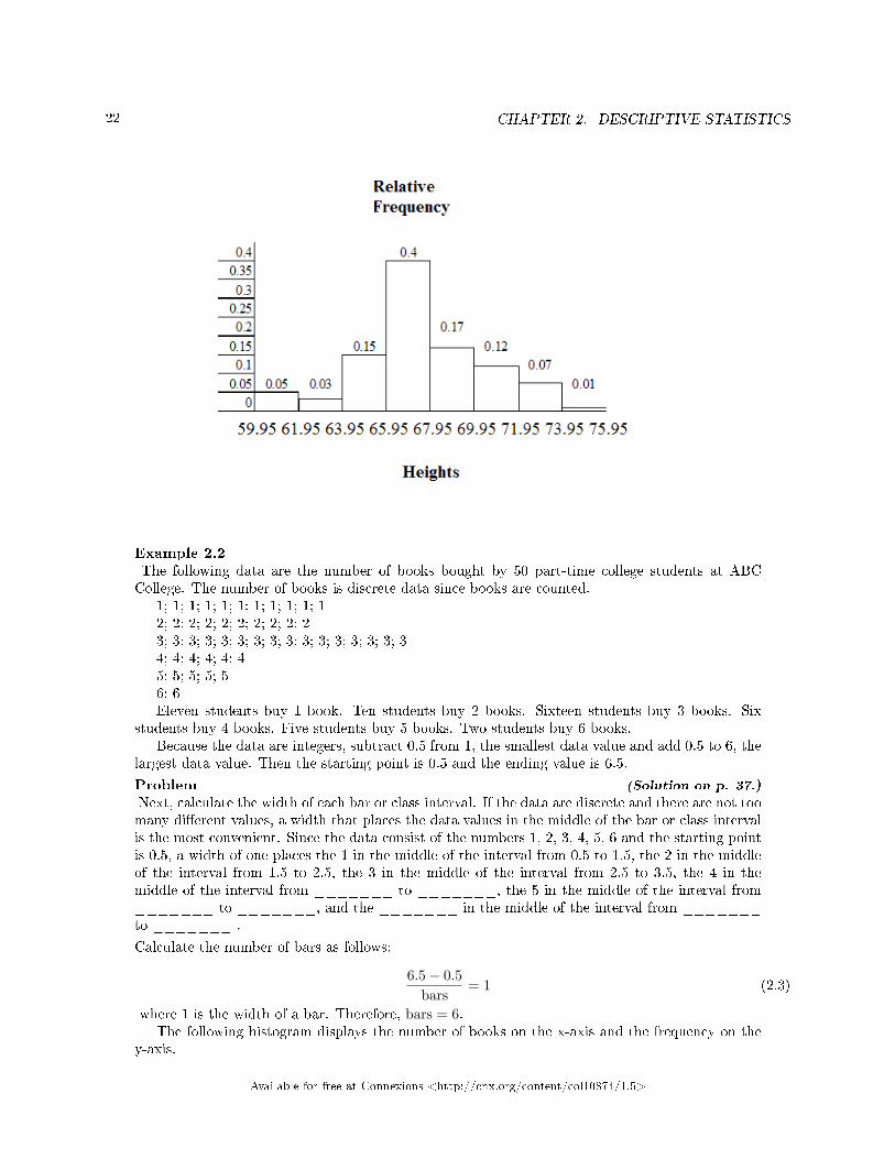
The following table represents the heights, in inches, of a sample of 100 male semiprofessional soccer players.
Frequency Table of Soccer Player Height
HEIGHTS(INCHES)
FREQUENCY RELATIVEFREQUENCY
CUMULATIVERELATIVEFREQUENCY
59.95 - 61.95 5 5100 = 0.05 0.05
61.95 - 63.95 3 3100 = 0.03 0.05 + 0.03 = 0.08
63.95 - 65.95 15 15100 = 0.15 0.08 + 0.15 = 0.23
65.95 - 67.95 40 40100 = 0.40 0.23 + 0.40 = 0.63
67.95 - 69.95 17 17100 = 0.17 0.63 + 0.17 = 0.80
69.95 - 71.95 12 12100 = 0.12 0.80 + 0.12 = 0.92
71.95 - 73.95 7 7100 = 0.07 0.92 + 0.07 = 0.99
73.95 - 75.95 1 1100 = 0.01 0.99 + 0.01 = 1.00
Total = 100 Total = 1.00
Table 1.17
The data in this table has been grouped into the following intervals:
• 59.95 - 61.95 inches• 61.95 - 63.95 inches• 63.95 - 65.95 inches• 65.95 - 67.95 inches• 67.95 - 69.95 inches• 69.95 - 71.95 inches• 71.95 - 73.95 inches
Available for free at Connexions <http://cnx.org/content/col10874/1.5>

16 CHAPTER 1. SAMPLING AND DATA
• 73.95 - 75.95 inches
note: This example is used again in the Descriptive Statistics (Section 2.1) chapter, where themethod used to compute the intervals will be explained.
In this sample, there are 5 players whose heights are between 59.95 - 61.95 inches, 3 players whose heightsfall within the interval 61.95 - 63.95 inches, 15 players whose heights fall within the interval 63.95 - 65.95inches, 40 players whose heights fall within the interval 65.95 - 67.95 inches, 17 players whose heights fallwithin the interval 67.95 - 69.95 inches, 12 players whose heights fall within the interval 69.95 - 71.95, 7players whose height falls within the interval 71.95 - 73.95, and 1 player whose height falls within the interval73.95 - 75.95. All heights fall between the endpoints of an interval and not at the endpoints.
Example 1.6From the table, �nd the percentage of heights that are less than 65.95 inches.
SolutionIf you look at the �rst, second, and third rows, the heights are all less than 65.95 inches. Thereare 5 + 3 + 15 = 23 males whose heights are less than 65.95 inches. The percentage of heights lessthan 65.95 inches is then 23
100 or 23%. This percentage is the cumulative relative frequency entry inthe third row.
Example 1.7From the table, �nd the percentage of heights that fall between 61.95 and 65.95 inches.
SolutionAdd the relative frequencies in the second and third rows: 0.03 + 0.15 = 0.18 or 18%.
Example 1.8Use the table of heights of the 100 male semiprofessional soccer players. Fill in the blanks andcheck your answers.
1. The percentage of heights that are from 67.95 to 71.95 inches is:2. The percentage of heights that are from 67.95 to 73.95 inches is:3. The percentage of heights that are more than 65.95 inches is:4. The number of players in the sample who are between 61.95 and 71.95 inches tall is:5. What kind of data are the heights?6. Describe how you could gather this data (the heights) so that the data are characteristic of
all male semiprofessional soccer players.
Remember, you count frequencies. To �nd the relative frequency, divide the frequency by thetotal number of data values. To �nd the cumulative relative frequency, add all of the previousrelative frequencies to the relative frequency for the current row.
Available for free at Connexions <http://cnx.org/content/col10874/1.5>

17
1.6.1 Optional Collaborative Classroom Exercise
Exercise 1.6.1In your class, have someone conduct a survey of the number of siblings (brothers and sisters) eachstudent has. Create a frequency table. Add to it a relative frequency column and a cumulativerelative frequency column. Answer the following questions:
1. What percentage of the students in your class has 0 siblings?2. What percentage of the students has from 1 to 3 siblings?3. What percentage of the students has fewer than 3 siblings?
Example 1.9Nineteen people were asked how many miles, to the nearest mile they commute to work each day.The data are as follows:
2; 5; 7; 3; 2; 10; 18; 15; 20; 7; 10; 18; 5; 12; 13; 12; 4; 5; 10The following table was produced:
Frequency of Commuting Distances
DATA FREQUENCY RELATIVEFREQUENCY
CUMULATIVERELATIVEFREQUENCY
3 3 319 0.1579
4 1 119 0.2105
5 3 319 0.1579
7 2 219 0.2632
10 3 419 0.4737
12 2 219 0.7895
13 1 119 0.8421
15 1 119 0.8948
18 1 119 0.9474
20 1 119 1.0000
Table 1.18
Problem (Solution on p. 18.)
1. Is the table correct? If it is not correct, what is wrong?2. True or False: Three percent of the people surveyed commute 3 miles. If the statement is not
correct, what should it be? If the table is incorrect, make the corrections.3. What fraction of the people surveyed commute 5 or 7 miles?4. What fraction of the people surveyed commute 12 miles or more? Less than 12 miles? Between
5 and 13 miles (does not include 5 and 13 miles)?
Available for free at Connexions <http://cnx.org/content/col10874/1.5>
18 CHAPTER 1. SAMPLING AND DATA
Solutions to Exercises in Chapter 1
Solution to Example 1.5, Problem (p. 6)Items 1, 5, 11, and 12 are quantitative discrete; items 4, 6, 10, and 14 are quantitative continuous; anditems 2, 3, 7, 8, 9, and 13 are qualitative.Solution to Example 1.8, Problem (p. 16)
1. 29%2. 36%3. 77%4. 875. quantitative continuous6. get rosters from each team and choose a simple random sample from each
Solution to Example 1.9, Problem (p. 17)
1. No. Frequency column sums to 18, not 19. Not all cumulative relative frequencies are correct.2. False. Frequency for 3 miles should be 1; for 2 miles (left out), 2. Cumulative relative frequency column
should read: 0.1052, 0.1579, 0.2105, 0.3684, 0.4737, 0.6316, 0.7368, 0.7895, 0.8421, 0.9474, 1.3. 5
194. 7
19 ,1219 ,
719
Available for free at Connexions <http://cnx.org/content/col10874/1.5>

Chapter 2
Descriptive Statistics
2.1 Descriptive Statistics: Introduction1
2.1.1 Student Learning Outcomes
By the end of this chapter, the student should be able to:
• Display data graphically and interpret graphs: stemplots, histograms and boxplots.• Recognize, describe, and calculate the measures of location of data: quartiles and percentiles.• Recognize, describe, and calculate the measures of the center of data: mean, median, and mode.• Recognize, describe, and calculate the measures of the spread of data: variance, standard deviation,
and range.
2.1.2 Introduction
Once you have collected data, what will you do with it? Data can be described and presented in manydi�erent formats. For example, suppose you are interested in buying a house in a particular area. You mayhave no clue about the house prices, so you might ask your real estate agent to give you a sample data set ofprices. Looking at all the prices in the sample often is overwhelming. A better way might be to look at themedian price and the variation of prices. The median and variation are just two ways that you will learn todescribe data. Your agent might also provide you with a graph of the data.
In this chapter, you will study numerical and graphical ways to describe and display your data. This areaof statistics is called "Descriptive Statistics". You will learn to calculate, and even more importantly, tointerpret these measurements and graphs.
2.2 Descriptive Statistics: Displaying Data2
A statistical graph is a tool that helps you learn about the shape or distribution of a sample. The graph canbe a more e�ective way of presenting data than a mass of numbers because we can see where data clustersand where there are only a few data values. Newspapers and the Internet use graphs to show trends and toenable readers to compare facts and �gures quickly.
Statisticians often graph data �rst to get a picture of the data. Then, more formal tools may be applied.Some of the types of graphs that are used to summarize and organize data are the dot plot, the bar chart,
the histogram, the stem-and-leaf plot, the frequency polygon (a type of broken line graph), pie charts, and
1This content is available online at <http://cnx.org/content/m16300/1.9/>.2This content is available online at <http://cnx.org/content/m16297/1.9/>.
Available for free at Connexions <http://cnx.org/content/col10874/1.5>
19

20 CHAPTER 2. DESCRIPTIVE STATISTICS
the boxplot. In this chapter, we will brie�y look at stem-and-leaf plots, line graphs and bar graphs. Ouremphasis will be on histograms and boxplots.
2.3 Descriptive Statistics: Histogram3
For most of the work you do in this book, you will use a histogram to display the data. One advantage ofa histogram is that it can readily display large data sets. A rule of thumb is to use a histogram when thedata set consists of 100 values or more.
A histogram consists of contiguous boxes. It has both a horizontal axis and a vertical axis. Thehorizontal axis is labeled with what the data represents (for instance, distance from your home to school).The vertical axis is labeled either Frequency or relative frequency. The graph will have the same shapewith either label. The histogram (like the stemplot) can give you the shape of the data, the center, and thespread of the data. (The next section tells you how to calculate the center and the spread.)
The relative frequency is equal to the frequency for an observed value of the data divided by the totalnumber of data values in the sample. (In the chapter on Sampling and Data (Section 1.1), we de�nedfrequency as the number of times an answer occurs.) If:
• f = frequency• n = total number of data values (or the sum of the individual frequencies), and• RF = relative frequency,
then:
RF =f
n(2.1)
For example, if 3 students in Mr. Ahab's English class of 40 students received from 90% to 100%, then,f = 3 , n = 40 , and RF = f
n = 340
= 0.075Seven and a half percent of the students received 90% to 100%. Ninety percent to 100 % are quantitative
measures.To construct a histogram, �rst decide how many bars or intervals, also called classes, represent the
data. Many histograms consist of from 5 to 15 bars or classes for clarity. Choose a starting point for the�rst interval to be less than the smallest data value. A convenient starting point is a lower value carriedout to one more decimal place than the value with the most decimal places. For example, if the value withthe most decimal places is 6.1 and this is the smallest value, a convenient starting point is 6.05 (6.1 - 0.05 =6.05). We say that 6.05 has more precision. If the value with the most decimal places is 2.23 and the lowestvalue is 1.5, a convenient starting point is 1.495 (1.5 - 0.005 = 1.495). If the value with the most decimalplaces is 3.234 and the lowest value is 1.0, a convenient starting point is 0.9995 (1.0 - .0005 = 0.9995). If allthe data happen to be integers and the smallest value is 2, then a convenient starting point is 1.5 (2 - 0.5= 1.5). Also, when the starting point and other boundaries are carried to one additional decimal place, nodata value will fall on a boundary.
Example 2.1The following data are the heights (in inches to the nearest half inch) of 100 male semiprofessionalsoccer players. The heights are continuous data since height is measured.
60; 60.5; 61; 61; 61.563.5; 63.5; 63.564; 64; 64; 64; 64; 64; 64; 64.5; 64.5; 64.5; 64.5; 64.5; 64.5; 64.5; 64.566; 66; 66; 66; 66; 66; 66; 66; 66; 66; 66.5; 66.5; 66.5; 66.5; 66.5; 66.5; 66.5; 66.5; 66.5; 66.5; 66.5;
67; 67; 67; 67; 67; 67; 67; 67; 67; 67; 67; 67; 67.5; 67.5; 67.5; 67.5; 67.5; 67.5; 67.568; 68; 69; 69; 69; 69; 69; 69; 69; 69; 69; 69; 69.5; 69.5; 69.5; 69.5; 69.5
3This content is available online at <http://cnx.org/content/m16298/1.14/>.
Available for free at Connexions <http://cnx.org/content/col10874/1.5>

21
70; 70; 70; 70; 70; 70; 70.5; 70.5; 70.5; 71; 71; 7172; 72; 72; 72.5; 72.5; 73; 73.574The smallest data value is 60. Since the data with the most decimal places has one decimal
(for instance, 61.5), we want our starting point to have two decimal places. Since the numbers 0.5,0.05, 0.005, etc. are convenient numbers, use 0.05 and subtract it from 60, the smallest value, forthe convenient starting point.
60 - 0.05 = 59.95 which is more precise than, say, 61.5 by one decimal place. The starting pointis, then, 59.95.
The largest value is 74. 74+ 0.05 = 74.05 is the ending value.Next, calculate the width of each bar or class interval. To calculate this width, subtract the
starting point from the ending value and divide by the number of bars (you must choose the numberof bars you desire). Suppose you choose 8 bars.
74.05− 59.958
= 1.76 (2.2)
note: We will round up to 2 and make each bar or class interval 2 units wide. Rounding up to 2 isone way to prevent a value from falling on a boundary. Rounding to the next number is necessaryeven if it goes against the standard rules of rounding. For this example, using 1.76 as the widthwould also work.
The boundaries are:
• 59.95• 59.95 + 2 = 61.95• 61.95 + 2 = 63.95• 63.95 + 2 = 65.95• 65.95 + 2 = 67.95• 67.95 + 2 = 69.95• 69.95 + 2 = 71.95• 71.95 + 2 = 73.95• 73.95 + 2 = 75.95
The heights 60 through 61.5 inches are in the interval 59.95 - 61.95. The heights that are 63.5 arein the interval 61.95 - 63.95. The heights that are 64 through 64.5 are in the interval 63.95 - 65.95.The heights 66 through 67.5 are in the interval 65.95 - 67.95. The heights 68 through 69.5 are inthe interval 67.95 - 69.95. The heights 70 through 71 are in the interval 69.95 - 71.95. The heights72 through 73.5 are in the interval 71.95 - 73.95. The height 74 is in the interval 73.95 - 75.95.
The following histogram displays the heights on the x-axis and relative frequency on the y-axis.
Available for free at Connexions <http://cnx.org/content/col10874/1.5>
22 CHAPTER 2. DESCRIPTIVE STATISTICS
Example 2.2The following data are the number of books bought by 50 part-time college students at ABCCollege. The number of books is discrete data since books are counted.
1; 1; 1; 1; 1; 1; 1; 1; 1; 1; 12; 2; 2; 2; 2; 2; 2; 2; 2; 23; 3; 3; 3; 3; 3; 3; 3; 3; 3; 3; 3; 3; 3; 3; 34; 4; 4; 4; 4; 45; 5; 5; 5; 56; 6Eleven students buy 1 book. Ten students buy 2 books. Sixteen students buy 3 books. Six
students buy 4 books. Five students buy 5 books. Two students buy 6 books.Because the data are integers, subtract 0.5 from 1, the smallest data value and add 0.5 to 6, the
largest data value. Then the starting point is 0.5 and the ending value is 6.5.
Problem (Solution on p. 37.)
Next, calculate the width of each bar or class interval. If the data are discrete and there are not toomany di�erent values, a width that places the data values in the middle of the bar or class intervalis the most convenient. Since the data consist of the numbers 1, 2, 3, 4, 5, 6 and the starting pointis 0.5, a width of one places the 1 in the middle of the interval from 0.5 to 1.5, the 2 in the middleof the interval from 1.5 to 2.5, the 3 in the middle of the interval from 2.5 to 3.5, the 4 in themiddle of the interval from _______ to _______, the 5 in the middle of the interval from_______ to _______, and the _______ in the middle of the interval from _______to _______ .
Calculate the number of bars as follows:
6.5− 0.5bars
= 1 (2.3)
where 1 is the width of a bar. Therefore, bars = 6.The following histogram displays the number of books on the x-axis and the frequency on the
y-axis.
Available for free at Connexions <http://cnx.org/content/col10874/1.5>

23
Using the TI-83, 83+, 84, 84+ Calculator InstructionsGo to the Appendix (14:Appendix) in the menu on the left. There are calculator instructions for enteringdata and for creating a customized histogram. Create the histogram for Example 2.
• Press Y=. Press CLEAR to clear out any equations.• Press STAT 1:EDIT. If L1 has data in it, arrow up into the name L1, press CLEAR and arrow down.
If necessary, do the same for L2.• Into L1, enter 1, 2, 3, 4, 5, 6• Into L2, enter 11, 10, 16, 6, 5, 2• Press WINDOW. Make Xmin = .5, Xmax = 6.5, Xscl = (6.5 - .5)/6, Ymin = -1, Ymax = 20, Yscl =
1, Xres = 1• Press 2nd Y=. Start by pressing 4:Plotso� ENTER.• Press 2nd Y=. Press 1:Plot1. Press ENTER. Arrow down to TYPE. Arrow to the 3rd picture
(histogram). Press ENTER.• Arrow down to Xlist: Enter L1 (2nd 1). Arrow down to Freq. Enter L2 (2nd 2).• Press GRAPH• Use the TRACE key and the arrow keys to examine the histogram.
2.3.1 Optional Collaborative Exercise
Count the money (bills and change) in your pocket or purse. Your instructor will record the amounts. As aclass, construct a histogram displaying the data. Discuss how many intervals you think is appropriate. Youmay want to experiment with the number of intervals. Discuss, also, the shape of the histogram.
Record the data, in dollars (for example, 1.25 dollars).Construct a histogram.
2.4 Descriptive Statistics: Measuring the Center of the Data4
The "center" of a data set is also a way of describing location. The two most widely used measures of the"center" of the data are the mean (average) and the median. To calculate the mean weight of 50 people,add the 50 weights together and divide by 50. To �nd the median weight of the 50 people, order the dataand �nd the number that splits the data into two equal parts (previously discussed under box plots in this
4This content is available online at <http://cnx.org/content/m17102/1.13/>.
Available for free at Connexions <http://cnx.org/content/col10874/1.5>

24 CHAPTER 2. DESCRIPTIVE STATISTICS
chapter). The median is generally a better measure of the center when there are extreme values or outliersbecause it is not a�ected by the precise numerical values of the outliers. The mean is the most commonmeasure of the center.
note: The words "mean" and "average" are often used interchangeably. The substitution of oneword for the other is common practice. The technical term is "arithmetic mean" and "average" istechnically a center location. However, in practice among non-statisticians, "average" is commonlyaccepted for "arithmetic mean."
The mean can also be calculated by multiplying each distinct value by its frequency and then dividing thesum by the total number of data values. The letter used to represent the sample mean is an x with a barover it (pronounced "x bar"): x.
The Greek letter µ (pronounced "mew") represents the population mean. One of the requirements forthe sample mean to be a good estimate of the population mean is for the sample taken to be truly random.
To see that both ways of calculating the mean are the same, consider the sample:1; 1; 1; 2; 2; 3; 4; 4; 4; 4; 4
x =1 + 1 + 1 + 2 + 2 + 3 + 4 + 4 + 4 + 4 + 4
11= 2.7 (2.4)
x =3× 1 + 2× 2 + 1× 3 + 5× 4
11= 2.7 (2.5)
In the second calculation for the sample mean, the frequencies are 3, 2, 1, and 5.You can quickly �nd the location of the median by using the expression n+1
2 .The letter n is the total number of data values in the sample. If n is an odd number, the median is the
middle value of the ordered data (ordered smallest to largest). If n is an even number, the median is equal tothe two middle values added together and divided by 2 after the data has been ordered. For example, if thetotal number of data values is 97, then n+1
2 = 97+12 = 49. The median is the 49th value in the ordered data.
If the total number of data values is 100, then n+12 = 100+1
2 = 50.5. The median occurs midway between the50th and 51st values. The location of the median and the value of the median are not the same. The uppercase letter M is often used to represent the median. The next example illustrates the location of the medianand the value of the median.
Example 2.3AIDS data indicating the number of months an AIDS patient lives after taking a new antibodydrug are as follows (smallest to largest):
3; 4; 8; 8; 10; 11; 12; 13; 14; 15; 15; 16; 16; 17; 17; 18; 21; 22; 22; 24; 24; 25; 26; 26; 27; 27; 29;29; 31; 32; 33; 33; 34; 34; 35; 37; 40; 44; 44; 47
Calculate the mean and the median.
SolutionThe calculation for the mean is:
x = [3+4+(8)(2)+10+11+12+13+14+(15)(2)+(16)(2)+...+35+37+40+(44)(2)+47]40 = 23.6
To �nd the median, M, �rst use the formula for the location. The location is:n+1
2 = 40+12 = 20.5
Starting at the smallest value, the median is located between the 20th and 21st values (the two24s):
3; 4; 8; 8; 10; 11; 12; 13; 14; 15; 15; 16; 16; 17; 17; 18; 21; 22; 22; 24; 24; 25; 26; 26; 27; 27; 29;29; 31; 32; 33; 33; 34; 34; 35; 37; 40; 44; 44; 47
M = 24+242 = 24
The median is 24.
Available for free at Connexions <http://cnx.org/content/col10874/1.5>
25
Using the TI-83,83+,84, 84+ CalculatorsCalculator Instructions are located in the menu item 14:Appendix (Notes for the TI-83, 83+, 84,84+ Calculators).
• Enter data into the list editor. Press STAT 1:EDIT• Put the data values in list L1.• Press STAT and arrow to CALC. Press 1:1-VarStats. Press 2nd 1 for L1 and ENTER.• Press the down and up arrow keys to scroll.
x = 23.6, M = 24
Example 2.4Suppose that, in a small town of 50 people, one person earns $5,000,000 per year and the other
49 each earn $30,000. Which is the better measure of the "center," the mean or the median?
Solutionx = 5000000+49×30000
50 = 129400M = 30000(There are 49 people who earn $30,000 and one person who earns $5,000,000.)The median is a better measure of the "center" than the mean because 49 of the values are
30,000 and one is 5,000,000. The 5,000,000 is an outlier. The 30,000 gives us a better sense of themiddle of the data.
Another measure of the center is the mode. The mode is the most frequent value. If a data set has twovalues that occur the same number of times, then the set is bimodal.
Example 2.5: Statistics exam scores for 20 students are as followsStatistics exam scores for 20 students are as follows:
50 ; 53 ; 59 ; 59 ; 63 ; 63 ; 72 ; 72 ; 72 ; 72 ; 72 ; 76 ; 78 ; 81 ; 83 ; 84 ; 84 ; 84 ; 90 ; 93
ProblemFind the mode.
SolutionThe most frequent score is 72, which occurs �ve times. Mode = 72.
Example 2.6Five real estate exam scores are 430, 430, 480, 480, 495. The data set is bimodal because the scores430 and 480 each occur twice.
When is the mode the best measure of the "center"? Consider a weight loss program thatadvertises a mean weight loss of six pounds the �rst week of the program. The mode might indicatethat most people lose two pounds the �rst week, making the program less appealing.
note: The mode can be calculated for qualitative data as well as for quantitative data.
Statistical software will easily calculate the mean, the median, and the mode. Some graphingcalculators can also make these calculations. In the real world, people make these calculationsusing software.
Available for free at Connexions <http://cnx.org/content/col10874/1.5>

26 CHAPTER 2. DESCRIPTIVE STATISTICS
2.4.1 The Law of Large Numbers and the Mean
The Law of Large Numbers says that if you take samples of larger and larger size from any population, thenthe mean x of the sample is very likely to get closer and closer to µ. This is discussed in more detail in TheCentral Limit Theorem.
note: The formula for the mean is located in the Summary of Formulas5 section course.
2.4.2 Sampling Distributions and Statistic of a Sampling Distribution
You can think of a sampling distribution as a relative frequency distribution with a great manysamples. (See Sampling and Data for a review of relative frequency). Suppose thirty randomly selectedstudents were asked the number of movies they watched the previous week. The results are in the relativefrequency table shown below.
# of movies Relative Frequency
0 5/30
1 15/30
2 6/30
3 4/30
4 1/30
Table 2.1
If you let the number of samples get very large (say, 300 million or more), the relativefrequency table becomes a relative frequency distribution.
A statistic is a number calculated from a sample. Statistic examples include the mean, the median andthe mode as well as others. The sample mean x is an example of a statistic which estimates the populationmean µ.
2.5 Descriptive Statistics: Skewness and the Mean, Median, and
Mode6
Consider the following data set:4 ; 5 ; 6 ; 6 ; 6 ; 7 ; 7 ; 7 ; 7 ; 7 ; 7 ; 8 ; 8 ; 8 ; 9 ; 10This data set produces the histogram shown below. Each interval has width one and each value is located
in the middle of an interval.
5"Descriptive Statistics: Summary of Formulas" <http://cnx.org/content/m16310/latest/>6This content is available online at <http://cnx.org/content/m17104/1.9/>.
Available for free at Connexions <http://cnx.org/content/col10874/1.5>

27
The histogram displays a symmetrical distribution of data. A distribution is symmetrical if a verticalline can be drawn at some point in the histogram such that the shape to the left and the right of the verticalline are mirror images of each other. The mean, the median, and the mode are each 7 for these data. Ina perfectly symmetrical distribution, the mean and the median are the same. This example hasone mode (unimodal) and the mode is the same as the mean and median. In a symmetrical distribution thathas two modes (bimodal), the two modes would be di�erent from the mean and median.
The histogram for the data:4 ; 5 ; 6 ; 6 ; 6 ; 7 ; 7 ; 7 ; 7 ; 8is not symmetrical. The right-hand side seems "chopped o�" compared to the left side. The shape
distribution is called skewed to the left because it is pulled out to the left.
The mean is 6.3, the median is 6.5, and the mode is 7. Notice that the mean is less than themedian and they are both less than the mode. The mean and the median both re�ect the skewingbut the mean more so.
The histogram for the data:6 ; 7 ; 7 ; 7 ; 7 ; 8 ; 8 ; 8 ; 9 ; 10is also not symmetrical. It is skewed to the right.
Available for free at Connexions <http://cnx.org/content/col10874/1.5>

28 CHAPTER 2. DESCRIPTIVE STATISTICS
The mean is 7.7, the median is 7.5, and the mode is 7. Of the three statistics, the mean is the largest,while the mode is the smallest. Again, the mean re�ects the skewing the most.
To summarize, generally if the distribution of data is skewed to the left, the mean is less than the median,which is often less than the mode. If the distribution of data is skewed to the right, the mode is often lessthan the median, which is less than the mean.
Skewness and symmetry become important when we discuss probability distributions in later chapters.
2.6 Descriptive Statistics: Measuring the Spread of the Data7
An important characteristic of any set of data is the variation in the data. In some data sets, the data valuesare concentrated closely near the mean; in other data sets, the data values are more widely spread out fromthe mean. The most common measure of variation, or spread, is the standard deviation.
The standard deviation is a number that measures how far data values are from their mean.The standard deviation
• provides a numerical measure of the overall amount of variation in a data set• can be used to determine whether a particular data value is close to or far from the mean
The standard deviation provides a measure of the overall variation in a data setThe standard deviation is always positive or 0. The standard deviation is small when the data are allconcentrated close to the mean, exhibiting little variation or spread. The standard deviation is larger whenthe data values are more spread out from the mean, exhibiting more variation.
Suppose that we are studying waiting times at the checkout line for customers at supermarket Aand supermarket B; the average wait time at both markets is 5 minutes. At market A, the standard de-viation for the waiting time is 2 minutes; at market B the standard deviation for the waiting time is 4 minutes.
Because market B has a higher standard deviation, we know that there is more variation in thewaiting times at market B. Overall, wait times at market B are more spread out from the average; waittimes at market A are more concentrated near the average.The standard deviation can be used to determine whether a data value is close to or far fromthe mean.Suppose that Rosa and Binh both shop at Market A. Rosa waits for 7 minutes and Binh waits for 1 minuteat the checkout counter. At market A, the mean wait time is 5 minutes and the standard deviation is 2minutes. The standard deviation can be used to determine whether a data value is close to or far from themean.Rosa waits for 7 minutes:
7This content is available online at <http://cnx.org/content/m17103/1.15/>.
Available for free at Connexions <http://cnx.org/content/col10874/1.5>

29
• 7 is 2 minutes longer than the average of 5; 2 minutes is equal to one standard deviation.• Rosa's wait time of 7 minutes is 2 minutes longer than the average of 5 minutes.• Rosa's wait time of 7 minutes is one standard deviation above the average of 5 minutes.
Binh waits for 1 minute.
• 1 is 4 minutes less than the average of 5; 4 minutes is equal to two standard deviations.• Binh's wait time of 1 minute is 4 minutes less than the average of 5 minutes.• Binh's wait time of 1 minute is two standard deviations below the average of 5 minutes.• A data value that is two standard deviations from the average is just on the borderline for what many
statisticians would consider to be far from the average. Considering data to be far from the mean if itis more than 2 standard deviations away is more of an approximate "rule of thumb" than a rigid rule.In general, the shape of the distribution of the data a�ects how much of the data is further away than2 standard deviations. (We will learn more about this in later chapters.)
The number line may help you understand standard deviation. If we were to put 5 and 7 on a numberline, 7 is to the right of 5. We say, then, that 7 is one standard deviation to the right of 5 because5 + (1) (2) = 7.
If 1 were also part of the data set, then 1 is two standard deviations to the left of 5 because5 + (−2) (2) = 1.
• In general, a value = mean + (#ofSTDEV)(standard deviation)• where #ofSTDEVs = the number of standard deviations• 7 is one standard deviation more than the mean of 5 because: 7=5+(1)(2)• 1 is two standard deviations less than the mean of 5 because: 1=5+(−2)(2)
The equation value = mean + (#ofSTDEVs)(standard deviation) can be expressed for a sampleand for a population:
• sample: x = x+ (#ofSTDEV) (s)• Population: x = µ+ (#ofSTDEV) (σ)
The lower case letter s represents the sample standard deviation and the Greek letter σ (sigma, lower case)represents the population standard deviation.
The symbol x is the sample mean and the Greek symbol µ is the population mean.Calculating the Standard DeviationIf x is a number, then the di�erence "x - mean" is called its deviation. In a data set, there are as manydeviations as there are items in the data set. The deviations are used to calculate the standard deviation.If the numbers belong to a population, in symbols a deviation is x − µ . For sample data, in symbols adeviation is x− x .
The procedure to calculate the standard deviation depends on whether the numbers are the entire pop-ulation or are data from a sample. The calculations are similar, but not identical. Therefore the symbol
Available for free at Connexions <http://cnx.org/content/col10874/1.5>
30 CHAPTER 2. DESCRIPTIVE STATISTICS
used to represent the standard deviation depends on whether it is calculated from a population or a sample.The lower case letter s represents the sample standard deviation and the Greek letter σ (sigma, lower case)represents the population standard deviation. If the sample has the same characteristics as the population,then s should be a good estimate of σ.
To calculate the standard deviation, we need to calculate the variance �rst. The variance is an averageof the squares of the deviations (the x− x values for a sample, or the x − µ values for a population).The symbol σ2 represents the population variance; the population standard deviation σ is the square rootof the population variance. The symbol s2 represents the sample variance; the sample standard deviation sis the square root of the sample variance. You can think of the standard deviation as a special average ofthe deviations.
If the numbers come from a census of the entire population and not a sample, when we calculatethe average of the squared deviations to �nd the variance, we divide by N, the number of items in thepopulation. If the data are from a sample rather than a population, when we calculate the average of thesquared deviations, we divide by n-1, one less than the number of items in the sample. You can see that inthe formulas below.Formulas for the Sample Standard Deviation
• s =√
Σ(x−x)2
n−1 or s =√
Σf ·(x−x)2
n−1
• For the sample standard deviation, the denominator is n-1, that is the sample size MINUS 1.
Formulas for the Population Standard Deviation
• σ =√
Σ(x−µ)2
N or σ =√
Σf ·(x−µ)2
N• For the population standard deviation, the denominator is N, the number of items in the population.
In these formulas, f represents the frequency with which a value appears. For example, if a value appearsonce, f is 1. If a value appears three times in the data set or population, f is 3.Sampling Variability of a StatisticThe statistic of a sampling distribution was discussed in Descriptive Statistics: Measuring the Centerof the Data. How much the statistic varies from one sample to another is known as the sampling vari-ability of a statistic. You typically measure the sampling variability of a statistic by its standard error.The standard error of the mean is an example of a standard error. It is a special standard deviation andis known as the standard deviation of the sampling distribution of the mean. You will cover the standarderror of the mean in The Central Limit Theorem (not now). The notation for the standard error of themean is σ√
nwhere σ is the standard deviation of the population and n is the size of the sample.
note: In practice, USE A CALCULATOR OR COMPUTER SOFTWARE TO CAL-CULATE THE STANDARD DEVIATION. If you are using a TI-83,83+,84+ calcula-tor, you need to select the appropriate standard deviation σx or sx from the summarystatistics. We will concentrate on using and interpreting the information that the standard devia-tion gives us. However you should study the following step-by-step example to help you understandhow the standard deviation measures variation from the mean.
Example 2.7In a �fth grade class, the teacher was interested in the average age and the sample standarddeviation of the ages of her students. The following data are the ages for a SAMPLE of n = 20�fth grade students. The ages are rounded to the nearest half year:
9 ; 9.5 ; 9.5 ; 10 ; 10 ; 10 ; 10 ; 10.5 ; 10.5 ; 10.5 ; 10.5 ; 11 ; 11 ; 11 ; 11 ; 11 ; 11 ; 11.5 ; 11.5 ;11.5
x =9 + 9.5× 2 + 10× 4 + 10.5× 4 + 11× 6 + 11.5× 3
20= 10.525 (2.6)
The average age is 10.53 years, rounded to 2 places.
Available for free at Connexions <http://cnx.org/content/col10874/1.5>

31
The variance may be calculated by using a table. Then the standard deviation is calculated bytaking the square root of the variance. We will explain the parts of the table after calculating s.
Data Freq. Deviations Deviations2 (Freq.)(Deviations2)
x f (x− x) (x− x)2 (f) (x− x)2
9 1 9− 10.525 = −1.525 (−1.525)2 = 2.325625 1× 2.325625 = 2.325625
9.5 2 9.5− 10.525 = −1.025 (−1.025)2 = 1.050625 2× 1.050625 = 2.101250
10 4 10− 10.525 = −0.525 (−0.525)2 = 0.275625 4× .275625 = 1.1025
10.5 4 10.5− 10.525 = −0.025 (−0.025)2 = 0.000625 4× .000625 = .0025
11 6 11− 10.525 = 0.475 (0.475)2 = 0.225625 6× .225625 = 1.35375
11.5 3 11.5− 10.525 = 0.975 (0.975)2 = 0.950625 3× .950625 = 2.851875
Table 2.2
The sample variance, s2, is equal to the sum of the last column (9.7375) divided by the totalnumber of data values minus one (20 - 1):
s2 = 9.737520−1 = 0.5125
The sample standard deviation s is equal to the square root of the sample variance:s =√
0.5125 = .0715891 Rounded to two decimal places, s = 0.72Typically, you do the calculation for the standard deviation on your calculator or
computer. The intermediate results are not rounded. This is done for accuracy.
Problem 1Verify the mean and standard deviation calculated above on your calculator or computer.
Solution
Using the TI-83,83+,84+ Calculators
� Enter data into the list editor. Press STAT 1:EDIT. If necessary, clear the lists by arrowingup into the name. Press CLEAR and arrow down.
� Put the data values (9, 9.5, 10, 10.5, 11, 11.5) into list L1 and the frequencies (1, 2, 4, 4, 6,3) into list L2. Use the arrow keys to move around.
� Press STAT and arrow to CALC. Press 1:1-VarStats and enter L1 (2nd 1), L2 (2nd 2). Donot forget the comma. Press ENTER.
� x=10.525� Use Sx because this is sample data (not a population): Sx=0.715891
• For the following problems, recall that value = mean + (#ofSTDEVs)(standard devi-ation)
• For a sample: x = x + (#ofSTDEVs)(s)• For a population: x = µ + (#ofSTDEVs)( σ)• For this example, use x = x + (#ofSTDEVs)(s) because the data is from a sample
Problem 2Find the value that is 1 standard deviation above the mean. Find (x+ 1s).
Solution(x+ 1s) = 10.53 + (1) (0.72) = 11.25
Available for free at Connexions <http://cnx.org/content/col10874/1.5>

32 CHAPTER 2. DESCRIPTIVE STATISTICS
Problem 3Find the value that is two standard deviations below the mean. Find (x− 2s).
Solution(x− 2s) = 10.53− (2) (0.72) = 9.09
Problem 4Find the values that are 1.5 standard deviations from (below and above) the mean.
Solution
• (x− 1.5s) = 10.53− (1.5) (0.72) = 9.45• (x+ 1.5s) = 10.53 + (1.5) (0.72) = 11.61
Explanation of the standard deviation calculation shown in the tableThe deviations show how spread out the data are about the mean. The data value 11.5 is farther from themean than is the data value 11. The deviations 0.97 and 0.47 indicate that. A positive deviation occurswhen the data value is greater than the mean. A negative deviation occurs when the data value is less thanthe mean; the deviation is -1.525 for the data value 9. If you add the deviations, the sum is alwayszero. (For this example, there are n=20 deviations.) So you cannot simply add the deviations to get thespread of the data. By squaring the deviations, you make them positive numbers, and the sum will also bepositive. The variance, then, is the average squared deviation.
The variance is a squared measure and does not have the same units as the data. Taking the square rootsolves the problem. The standard deviation measures the spread in the same units as the data.
Notice that instead of dividing by n=20, the calculation divided by n-1=20-1=19 because the data is asample. For the sample variance, we divide by the sample size minus one (n− 1). Why not divide byn? The answer has to do with the population variance. The sample variance is an estimate of thepopulation variance. Based on the theoretical mathematics that lies behind these calculations, dividingby (n− 1) gives a better estimate of the population variance.
note: Your concentration should be on what the standard deviation tells us about the data. Thestandard deviation is a number which measures how far the data are spread from the mean. Let acalculator or computer do the arithmetic.
The standard deviation, s or σ, is either zero or larger than zero. When the standard deviation is 0, there isno spread; that is, the all the data values are equal to each other. The standard deviation is small when thedata are all concentrated close to the mean, and is larger when the data values show more variation fromthe mean. When the standard deviation is a lot larger than zero, the data values are very spread out aboutthe mean; outliers can make s or σ very large.
The standard deviation, when �rst presented, can seem unclear. By graphing your data, you can get abetter "feel" for the deviations and the standard deviation. You will �nd that in symmetrical distributions,the standard deviation can be very helpful but in skewed distributions, the standard deviation may not bemuch help. The reason is that the two sides of a skewed distribution have di�erent spreads. In a skeweddistribution, it is better to look at the �rst quartile, the median, the third quartile, the smallest value, andthe largest value. Because numbers can be confusing, always graph your data.
note: The formula for the standard deviation is at the end of the chapter.
Available for free at Connexions <http://cnx.org/content/col10874/1.5>

33
Example 2.8Use the following data (�rst exam scores) from Susan Dean's spring pre-calculus class:
33; 42; 49; 49; 53; 55; 55; 61; 63; 67; 68; 68; 69; 69; 72; 73; 74; 78; 80; 83; 88; 88; 88; 90; 92; 94;94; 94; 94; 96; 100
a. Create a chart containing the data, frequencies, relative frequencies, and cumulative relativefrequencies to three decimal places.
b. Calculate the following to one decimal place using a TI-83+ or TI-84 calculator:
i. The sample meanii. The sample standard deviationiii. The medianiv. The �rst quartilev. The third quartilevi. IQR
c. Construct a box plot and a histogram on the same set of axes. Make comments about the boxplot, the histogram, and the chart.
Solution
a.Data Frequency Relative Frequency Cumulative Relative Frequency
33 1 0.032 0.032
42 1 0.032 0.064
49 2 0.065 0.129
53 1 0.032 0.161
55 2 0.065 0.226
61 1 0.032 0.258
63 1 0.032 0.29
67 1 0.032 0.322
68 2 0.065 0.387
69 2 0.065 0.452
72 1 0.032 0.484
73 1 0.032 0.516
74 1 0.032 0.548
78 1 0.032 0.580
80 1 0.032 0.612
83 1 0.032 0.644
88 3 0.097 0.741
90 1 0.032 0.773
92 1 0.032 0.805
94 4 0.129 0.934
96 1 0.032 0.966
100 1 0.032 0.998 (Why isn't this value 1?)
Available for free at Connexions <http://cnx.org/content/col10874/1.5>

34 CHAPTER 2. DESCRIPTIVE STATISTICS
Table 2.3
b. i. The sample mean = 73.5ii. The sample standard deviation = 17.9iii. The median = 73iv. The �rst quartile = 61v. The third quartile = 90vi. IQR = 90 - 61 = 29
c. The x-axis goes from 32.5 to 100.5; y-axis goes from -2.4 to 15 for the histogram; number ofintervals is 5 for the histogram so the width of an interval is (100.5 - 32.5) divided by 5 which isequal to 13.6. Endpoints of the intervals: starting point is 32.5, 32.5+13.6 = 46.1, 46.1+13.6= 59.7, 59.7+13.6 = 73.3, 73.3+13.6 = 86.9, 86.9+13.6 = 100.5 = the ending value; No datavalues fall on an interval boundary.
Figure 2.1
The long left whisker in the box plot is re�ected in the left side of the histogram. The spread ofthe exam scores in the lower 50% is greater (73 - 33 = 40) than the spread in the upper 50% (100- 73 = 27). The histogram, box plot, and chart all re�ect this. There are a substantial number ofA and B grades (80s, 90s, and 100). The histogram clearly shows this. The box plot shows us thatthe middle 50% of the exam scores (IQR = 29) are Ds, Cs, and Bs. The box plot also shows usthat the lower 25% of the exam scores are Ds and Fs.
Comparing Values from Di�erent Data SetsThe standard deviation is useful when comparing data values that come from di�erent data sets. If the datasets have di�erent means and standard deviations, it can be misleading to compare the data values directly.
• For each data value, calculate how many standard deviations the value is away from its mean.
Available for free at Connexions <http://cnx.org/content/col10874/1.5>
35
• Use the formula: value = mean + (#ofSTDEVs)(standard deviation); solve for #ofSTDEVs.• #ofSTDEVs = value−mean
standard deviation• Compare the results of this calculation.
#ofSTDEVs is often called a "z-score"; we can use the symbol z. In symbols, the formulas become:
Sample x = x + z s z = x−xs
Population x = µ + z σ z = x−µσ
Table 2.4
Example 2.9Two students, John and Ali, from di�erent high schools, wanted to �nd out who had the highestG.P.A. when compared to his school. Which student had the highest G.P.A. when compared to hisschool?
Student GPA School Mean GPA School Standard Deviation
John 2.85 3.0 0.7
Ali 77 80 10
Table 2.5
SolutionFor each student, determine how many standard deviations (#ofSTDEVs) his GPA is away fromthe average, for his school. Pay careful attention to signs when comparing and interpreting theanswer.
#ofSTDEVs = value−meanstandard deviation ; z = x−µ
σFor John, z = #ofSTDEVs = 2.85−3.0
0.7 = −0.21For Ali, z = #ofSTDEVs = 77−80
10 = −0.3John has the better G.P.A. when compared to his school because his G.P.A. is 0.21 standard
deviations below his school's mean while Ali's G.P.A. is 0.3 standard deviations below hisschool's mean.
John's z-score of −0.21 is higher than Ali's z-score of −0.3 . For GPA, higher values arebetter, so we conclude that John has the better GPA when compared to his school.
The following lists give a few facts that provide a little more insight into what the standard deviation tellsus about the distribution of the data.
For ANY data set, no matter what the distribution of the data is:
• At least 75% of the data is within 2 standard deviations of the mean.• At least 89% of the data is within 3 standard deviations of the mean.• At least 95% of the data is within 4 1/2 standard deviations of the mean.• This is known as Chebyshev's Rule.
For data having a distribution that is MOUND-SHAPED and SYMMETRIC:
• Approximately 68% of the data is within 1 standard deviation of the mean.
Available for free at Connexions <http://cnx.org/content/col10874/1.5>

36 CHAPTER 2. DESCRIPTIVE STATISTICS
• Approximately 95% of the data is within 2 standard deviations of the mean.• More than 99% of the data is within 3 standard deviations of the mean.• This is known as the Empirical Rule.• It is important to note that this rule only applies when the shape of the distribution of the data
is mound-shaped and symmetric. We will learn more about this when studying the "Normal" or"Gaussian" probability distribution in later chapters.
**With contributions from Roberta Bloom
Available for free at Connexions <http://cnx.org/content/col10874/1.5>

37
Solutions to Exercises in Chapter 2
Solution to Example 2.2, Problem (p. 22)
• 3.5 to 4.5• 4.5 to 5.5• 6• 5.5 to 6.5
Available for free at Connexions <http://cnx.org/content/col10874/1.5>

38 CHAPTER 2. DESCRIPTIVE STATISTICS
Available for free at Connexions <http://cnx.org/content/col10874/1.5>
Chapter 3
The Normal Distribution
3.1 Normal Distribution: Introduction1
3.1.1 Student Learning Outcomes
By the end of this chapter, the student should be able to:
• Recognize the normal probability distribution and apply it appropriately.• Recognize the standard normal probability distribution and apply it appropriately.• Compare normal probabilities by converting to the standard normal distribution.
3.1.2 Introduction
The normal, a continuous distribution, is the most important of all the distributions. It is widely usedand even more widely abused. Its graph is bell-shaped. You see the bell curve in almost all disciplines.Some of these include psychology, business, economics, the sciences, nursing, and, of course, mathematics.Some of your instructors may use the normal distribution to help determine your grade. Most IQ scores arenormally distributed. Often real estate prices �t a normal distribution. The normal distribution is extremelyimportant but it cannot be applied to everything in the real world.
In this chapter, you will study the normal distribution, the standard normal, and applications associatedwith them.
3.1.3 Optional Collaborative Classroom Activity
Your instructor will record the heights of both men and women in your class, separately. Draw histogramsof your data. Then draw a smooth curve through each histogram. Is each curve somewhat bell-shaped?Do you think that if you had recorded 200 data values for men and 200 for women that the curves wouldlook bell-shaped? Calculate the mean for each data set. Write the means on the x-axis of the appropriategraph below the peak. Shade the approximate area that represents the probability that one randomly chosenmale is taller than 72 inches. Shade the approximate area that represents the probability that one randomlychosen female is shorter than 60 inches. If the total area under each curve is one, does either probabilityappear to be more than 0.5?
The normal distribution has two parameters (two numerical descriptive measures), the mean (µ) and thestandard deviation (σ). If X is a quantity to be measured that has a normal distribution with mean (µ) andthe standard deviation (σ), we designate this by writing
NORMAL:X∼N (µ, σ)
1This content is available online at <http://cnx.org/content/m16979/1.12/>.
Available for free at Connexions <http://cnx.org/content/col10874/1.5>
39

40 CHAPTER 3. THE NORMAL DISTRIBUTION
The probability density function is a rather complicated function. Do not memorize it. It is notnecessary.
f (x) = 1σ·√
2·π · e− 1
2 ·( x−µσ )2
The cumulative distribution function is P (X < x) . It is calculated either by a calculator or a computeror it is looked up in a table. Technology has made the tables basically obsolete. For that reason, as well asthe fact that there are various table formats, we are not including table instructions in this chapter. See theNOTE in this chapter in Calculation of Probabilities.
The curve is symmetrical about a vertical line drawn through the mean, µ. In theory, the mean is thesame as the median since the graph is symmetric about µ. As the notation indicates, the normal distributiondepends only on the mean and the standard deviation. Since the area under the curve must equal one, achange in the standard deviation, σ, causes a change in the shape of the curve; the curve becomes fatteror skinnier depending on σ. A change in µ causes the graph to shift to the left or right. This means thereare an in�nite number of normal probability distributions. One of special interest is called the standardnormal distribution.
3.2 Normal Distribution: Standard Normal Distribution2
The standard normal distribution is a normal distribution of standardized values called z-scores.A z-score is measured in units of the standard deviation. For example, if the mean of a normaldistribution is 5 and the standard deviation is 2, the value 11 is 3 standard deviations above (or to the rightof) the mean. The calculation is:
x = µ + (z)σ = 5 + (3) (2) = 11 (3.1)
The z-score is 3.The mean for the standard normal distribution is 0 and the standard deviation is 1. The transformationz = x−µ
σ produces the distribution Z∼ N (0, 1) . The value x comes from a normal distributionwith mean µ and standard deviation σ.
3.3 Normal Distribution: Z-scores3
If X is a normally distributed random variable and X∼N (µ, σ), then the z-score is:
z =x− µσ
(3.2)
The z-score tells you how many standard deviations that the value x is above (to the right of)or below (to the left of) the mean, µ. Values of x that are larger than the mean have positive z-scoresand values of x that are smaller than the mean have negative z-scores. If x equals the mean, then x has az-score of 0.
2This content is available online at <http://cnx.org/content/m16986/1.7/>.3This content is available online at <http://cnx.org/content/m16991/1.10/>.
Available for free at Connexions <http://cnx.org/content/col10874/1.5>

41
Example 3.1Suppose X ∼ N (5, 6). This says that X is a normally distributed random variable with meanµ = 5 and standard deviation σ = 6. Suppose x = 17. Then:
z =x− µσ
=17− 5
6= 2 (3.3)
This means that x = 17 is 2 standard deviations (2σ) above or to the right of the mean µ = 5.The standard deviation is σ = 6.
Notice that:
5 + 2 · 6 = 17 (The pattern is µ+ zσ = x.) (3.4)
Now suppose x = 1. Then:
z =x− µσ
=1− 5
6= −0.67 (rounded to two decimal places) (3.5)
This means that x = 1 is 0.67 standard deviations (− 0.67σ) below or to the left ofthe mean µ = 5. Notice that:
5 + (−0.67) (6) is approximately equal to 1 (This has the pattern µ+ (−0.67)σ = 1 )Summarizing, when z is positive, x is above or to the right of µ and when z is negative, x is to
the left of or below µ.
Example 3.2Some doctors believe that a person can lose 5 pounds, on the average, in a month by reducinghis/her fat intake and by exercising consistently. Suppose weight loss has a normal distribution.Let X = the amount of weight lost (in pounds) by a person in a month. Use a standard deviationof 2 pounds. X∼N (5, 2). Fill in the blanks.
Problem 1 (Solution on p. 54.)
Suppose a person lost 10 pounds in a month. The z-score when x = 10 pounds is z = 2.5 (verify).This z-score tells you that x = 10 is ________ standard deviations to the ________ (rightor left) of the mean _____ (What is the mean?).
Problem 2 (Solution on p. 54.)
Suppose a person gained 3 pounds (a negative weight loss). Then z = __________. Thisz-score tells you that x = −3 is ________ standard deviations to the __________ (rightor left) of the mean.
Suppose the random variables X and Y have the following normal distributions: X ∼N (5, 6) andY ∼ N (2, 1). If x = 17, then z = 2. (This was previously shown.) If y = 4, what is z?
z =y − µσ
=4− 2
1= 2 where µ=2 and σ=1. (3.6)
The z-score for y = 4 is z = 2. This means that 4 is z = 2 standard deviations to the right ofthe mean. Therefore, x = 17 and y = 4 are both 2 (of their) standard deviations to the right oftheir respective means.
The z-score allows us to compare data that are scaled di�erently. To understand theconcept, suppose X ∼N (5, 6) represents weight gains for one group of people who are trying togain weight in a 6 week period and Y ∼N (2, 1) measures the same weight gain for a second groupof people. A negative weight gain would be a weight loss. Since x = 17 and y = 4 are each 2standard deviations to the right of their means, they represent the same weight gain relative totheir means.
The Empirical RuleIf X is a random variable and has a normal distribution with mean µ and standard deviation σ then theEmpirical Rule says (See the �gure below)
Available for free at Connexions <http://cnx.org/content/col10874/1.5>

42 CHAPTER 3. THE NORMAL DISTRIBUTION
• About 68.27% of the x values lie between -1σ and +1σ of the mean µ (within 1 standard deviation ofthe mean).
• About 95.45% of the x values lie between -2σ and +2σ of the mean µ (within 2 standard deviations ofthe mean).
• About 99.73% of the x values lie between -3σ and +3σ of the mean µ (within 3 standard deviations ofthe mean). Notice that almost all the x values lie within 3 standard deviations of the mean.
• The z-scores for +1σ and �1σ are +1 and -1, respectively.• The z-scores for +2σ and �2σ are +2 and -2, respectively.• The z-scores for +3σ and �3σ are +3 and -3 respectively.
The Empirical Rule is also known as the 68-95-99.7 Rule.
Example 3.3Suppose X has a normal distribution with mean 50 and standard deviation 6.
• About 68.27% of the x values lie between -1σ = (-1)(6) = -6 and 1σ = (1)(6) = 6 of the mean50. The values 50 - 6 = 44 and 50 + 6 = 56 are within 1 standard deviation of the mean 50.The z-scores are -1 and +1 for 44 and 56, respectively.
• About 95.45% of the x values lie between -2σ = (-2)(6) = -12 and 2σ = (2)(6) = 12 of themean 50. The values 50 - 12 = 38 and 50 + 12 = 62 are within 2 standard deviations of themean 50. The z-scores are -2 and 2 for 38 and 62, respectively.
• About 99.73% of the x values lie between -3σ = (-3)(6) = -18 and 3σ = (3)(6) = 18 of themean 50. The values 50 - 18 = 32 and 50 + 18 = 68 are within 3 standard deviations of themean 50. The z-scores are -3 and +3 for 32 and 68, respectively.
3.4 Normal Distribution: Areas to the Left and Right of x4
The arrow in the graph below points to the area to the left of x. This area is represented by the probabilityP (X < x). Normal tables, computers, and calculators provide or calculate the probability P (X < x).
4This content is available online at <http://cnx.org/content/m16976/1.5/>.
Available for free at Connexions <http://cnx.org/content/col10874/1.5>

43
The area to the right is then P (X > x) = 1− P (X < x).Remember, P (X < x) = Area to the left of the vertical line through x.P (X > x) = 1− P (X < x) =. Area to the right of the vertical line through xP (X < x) is the same as P (X ≤ x) and P (X > x) is the same as P (X ≥ x) for continuous distributions.
3.5 Normal Distribution: Calculations of Probabilities5
Probabilities are calculated by using technology. There are instructions in the chapter for the TI-83+ andTI-84 calculators.
note: In the Table of Contents for Collaborative Statistics, entry 15. Tables has a link to atable of normal probabilities. Use the probability tables if so desired, instead of a calculator. Thetables include instructions for how to use then.
Example 3.4If the area to the left is 0.0228, then the area to the right is 1− 0.0228 = 0.9772.
Example 3.5The �nal exam scores in a statistics class were normally distributed with a mean of 63 and astandard deviation of 5.
Problem 1Find the probability that a randomly selected student scored more than 65 on the exam.
SolutionLet X = a score on the �nal exam. X∼N (63, 5), where µ = 63 and σ = 5
Draw a graph.Then, �nd P (x > 65).P (x > 65) = 0.3446 (calculator or computer)
The probability that one student scores more than 65 is 0.3446.Using the TI-83+ or the TI-84 calculators, the calculation is as follows. Go into 2nd DISTR.After pressing 2nd DISTR, press 2:normalcdf.The syntax for the instructions are shown below.normalcdf(lower value, upper value, mean, standard deviation) For this problem: normal-
cdf(65,1E99,63,5) = 0.3446. You get 1E99 ( = 1099) by pressing 1, the EE key (a 2nd key) and then
5This content is available online at <http://cnx.org/content/m16977/1.12/>.
Available for free at Connexions <http://cnx.org/content/col10874/1.5>

44 CHAPTER 3. THE NORMAL DISTRIBUTION
99. Or, you can enter 10^99 instead. The number 1099 is way out in the right tail of the normalcurve. We are calculating the area between 65 and 1099. In some instances, the lower number ofthe area might be -1E99 ( = −1099). The number −1099 is way out in the left tail of the normalcurve.
Historical Note: The TI probability program calculates a z-score and then the probability fromthe z-score. Before technology, the z-score was looked up in a standard normal probability table(because the math involved is too cumbersome) to �nd the probability. In this example, a standardnormal table with area to the left of the z-score was used. You calculate the z-score and look upthe area to the left. The probability is the area to the right.
z = 65−635 = 0.4 . Area to the left is 0.6554. P (x > 65) = P (z > 0.4) = 1− 0.6554 = 0.3446
Problem 2Find the probability that a randomly selected student scored less than 85.
SolutionDraw a graph.
Then �nd P (x < 85). Shade the graph. P (x < 85) = 1 (calculator or computer)The probability that one student scores less than 85 is approximately 1 (or 100%).The TI-instructions and answer are as follows:normalcdf(0,85,63,5) = 1 (rounds to 1)
Problem 3Find the 90th percentile (that is, �nd the score k that has 90 % of the scores below k and 10% ofthe scores above k).
SolutionFind the 90th percentile. For each problem or part of a problem, draw a new graph. Draw thex-axis. Shade the area that corresponds to the 90th percentile.
Let k = the 90th percentile. k is located on the x-axis. P (x < k) is the area to the left ofk. The 90th percentile k separates the exam scores into those that are the same or lower than kand those that are the same or higher. Ninety percent of the test scores are the same or lower thank and 10% are the same or higher. k is often called a critical value.
k = 69.4 (calculator or computer)
The 90th percentile is 69.4. This means that 90% of the test scores fall at or below 69.4 and 10%fall at or above. For the TI-83+ or TI-84 calculators, use invNorm in 2nd DISTR. invNorm(area tothe left, mean, standard deviation) For this problem, invNorm(0.90,63,5) = 69.4
Problem 4Find the 70th percentile (that is, �nd the score k such that 70% of scores are below k and 30% ofthe scores are above k).
Available for free at Connexions <http://cnx.org/content/col10874/1.5>

45
SolutionFind the 70th percentile.
Draw a new graph and label it appropriately. k = 65.6The 70th percentile is 65.6. This means that 70% of the test scores fall at or below 65.5 and
30% fall at or above.invNorm(0.70,63,5) = 65.6
Example 3.6A computer is used for o�ce work at home, research, communication, personal �nances, education,entertainment, social networking and a myriad of other things. Suppose that the average numberof hours a household personal computer is used for entertainment is 2 hours per day. Assume thetimes for entertainment are normally distributed and the standard deviation for the times is halfan hour.
Problem 1Find the probability that a household personal computer is used between 1.8 and 2.75 hours perday.
SolutionLet X = the amount of time (in hours) a household personal computer is used for entertainment.x∼N (2, 0.5) where µ = 2 and σ = 0.5.
Find P (1.8 < x < 2.75).The probability for which you are looking is the area between x = 1.8 and x =
2.75. P (1.8 < x < 2.75) = 0.5886
normalcdf(1.8,2.75,2,0.5) = 0.5886The probability that a household personal computer is used between 1.8 and 2.75 hours per day
for entertainment is 0.5886.
Problem 2Find the maximum number of hours per day that the bottom quartile of households use a personalcomputer for entertainment.
SolutionTo �nd the maximum number of hours per day that the bottom quartile of households uses apersonal computer for entertainment, �nd the 25th percentile, k, where P (x < k) = 0.25.
Available for free at Connexions <http://cnx.org/content/col10874/1.5>

46 CHAPTER 3. THE NORMAL DISTRIBUTION
invNorm(0.25,2,.5) = 1.66The maximum number of hours per day that the bottom quartile of households uses a personal
computer for entertainment is 1.66 hours.
3.6 Central Limit Theorem: Central Limit Theorem for Sample
Means6
Suppose X is a random variable with a distribution that may be known or unknown (it can be any distri-bution). Using a subscript that matches the random variable, suppose:
a. µX = the mean of Xb. σX = the standard deviation of X
If you draw random samples of size n, then as n increases, the random variable X which consists of samplemeans, tends to be normally distributed and
X ∼ N(µX ,
σX√n
)The Central Limit Theorem for Sample Means says that if you keep drawing larger and larger
samples (like rolling 1, 2, 5, and, �nally, 10 dice) and calculating their means the sample meansform their own normal distribution (the sampling distribution). The normal distribution has the samemean as the original distribution and a variance that equals the original variance divided by n, the sam-ple size. n is the number of values that are averaged together not the number of times the experiment is done.
To put it more formally, if you draw random samples of size n,the distribution of the random vari-able X, which consists of sample means, is called the sampling distribution of the mean. The samplingdistribution of the mean approaches a normal distribution as n, the sample size, increases.
The random variable X has a di�erent z-score associated with it than the random variable X. x is thevalue of X in one sample.
z =x− µX(σX√n
) (3.7)
µX is both the average of X and of X.σX = σX√
n= standard deviation of X and is called the standard error of the mean.
Example 3.7An unknown distribution has a mean of 90 and a standard deviation of 15. Samples of size n = 25are drawn randomly from the population.
Problem 1Find the probability that the sample mean is between 85 and 92.
SolutionLet X = one value from the original unknown population. The probability question asks you to�nd a probability for the sample mean.
Let X = the mean of a sample of size 25. Since µX = 90, σX = 15, and n = 25;then X ∼ N
(90, 15√
25
)Find P (85 < x < 92) Draw a graph.
6This content is available online at <http://cnx.org/content/m16947/1.23/>.
Available for free at Connexions <http://cnx.org/content/col10874/1.5>

47
P (85 < x < 92) = 0.6997The probability that the sample mean is between 85 and 92 is 0.6997.
TI-83 or 84: normalcdf(lower value, upper value, mean, standard error of the mean)The parameter list is abbreviated (lower value, upper value, µ, σ√
n)
normalcdf
(85, 92, 90, 15√
25
)= 0.6997
Problem 2Find the value that is 2 standard deviations above the expected value (it is 90) of the sample mean.
SolutionTo �nd the value that is 2 standard deviations above the expected value 90, use the formula
value = µX + (#ofSTDEVs)(σX√n
)value = 90 + 2 · 15√
25= 96
So, the value that is 2 standard deviations above the expected value is 96.
Example 3.8The length of time, in hours, it takes an "over 40" group of people to play one soccer match isnormally distributed with a mean of 2 hours and a standard deviation of 0.5 hours. Asample of size n = 50 is drawn randomly from the population.
ProblemFind the probability that the sample mean is between 1.8 hours and 2.3 hours.
SolutionLet X = the time, in hours, it takes to play one soccer match.
The probability question asks you to �nd a probability for the sample mean time, in hours,it takes to play one soccer match.
Let X = the mean time, in hours, it takes to play one soccer match.
If µX = _________, σX = __________, and n = ___________, thenX ∼ N(______, ______) by the Central Limit Theorem for Means.
µX = 2, σX = 0.5, n = 50, and X ∼ N(
2 , 0.5√50
)Find P (1.8 < x < 2.3). Draw a graph.P (1.8 < x < 2.3) = 0.9977
Available for free at Connexions <http://cnx.org/content/col10874/1.5>

48 CHAPTER 3. THE NORMAL DISTRIBUTION
normalcdf
(1.8, 2.3, 2, .5√
50
)= 0.9977
The probability that the mean time is between 1.8 hours and 2.3 hours is ______.
3.7 Central Limit Theorem: Using the Central Limit Theorem7
It is important for you to understand when to use the CLT. If you are being asked to �nd the probabilityof the mean, use the CLT for the mean. If you are being asked to �nd the probability of a sum or total, usethe CLT for sums. This also applies to percentiles for means and sums.
note: If you are being asked to �nd the probability of an individual value, do not use the CLT.Use the distribution of its random variable.
3.7.1 Examples of the Central Limit Theorem
Law of Large NumbersThe Law of Large Numbers says that if you take samples of larger and larger size from any population,
then the mean x of the sample tends to get closer and closer to µ. From the Central Limit Theorem, weknow that as n gets larger and larger, the sample means follow a normal distribution. The larger n gets,the smaller the standard deviation gets. (Remember that the standard deviation for X is σ√
n.) This means
that the sample mean x must be close to the population mean µ. We can say that µ is the value that thesample means approach as n gets larger. The Central Limit Theorem illustrates the Law of Large Numbers.
Central Limit Theorem for the Mean and Sum Examples
Example 3.9A study involving stress is done on a college campus among the students. The stress scoresfollow a uniform distribution with the lowest stress score equal to 1 and the highest equal to5. Using a sample of 75 students, �nd:
1. The probability that the mean stress score for the 75 students is less than 2.2. The 90th percentile for the mean stress score for the 75 students.3. The probability that the total of the 75 stress scores is less than 200.4. The 90th percentile for the total stress score for the 75 students.
Let X = one stress score.Problems 1. and 2. ask you to �nd a probability or a percentile for a mean. Problems 3 and 4
ask you to �nd a probability or a percentile for a total or sum. The sample size, n, is equal to 75.Since the individual stress scores follow a uniform distribution, X ∼ U (1, 5) where a = 1 and
b = 5 (See Continuous Random Variables8 for the uniform).µX = a+b
2 = 1+52 = 3
σX =√
(b−a)2
12 =√
(5−1)2
12 = 1.15For problems 1. and 2., let X = the mean stress score for the 75 students. Then,
X ∼ N(
3, 1.15√75
)where n = 75.
Problem 1Find P (x < 2). Draw the graph.
7This content is available online at <http://cnx.org/content/m16958/1.21/>.8"Continuous Random Variables: Introduction" <http://cnx.org/content/m16808/latest/>
Available for free at Connexions <http://cnx.org/content/col10874/1.5>

49
SolutionP (x < 2) = 0
The probability that the mean stress score is less than 2 is about 0.
normalcdf
(1, 2, 3, 1.15√
75
)= 0
Reminder: The smallest stress score is 1. Therefore, the smallest mean for 75 stress scores is 1.
Problem 2Find the 90th percentile for the mean of 75 stress scores. Draw a graph.
SolutionLet k = the 90th precentile.
Find k where P (x < k) = 0.90.k = 3.2
The 90th percentile for the mean of 75 scores is about 3.2. This tells us that 90% of all themeans of 75 stress scores are at most 3.2 and 10% are at least 3.2.
invNorm
(.90, 3, 1.15√
75
)= 3.2
For problems c and d, let ΣX = the sum of the 75 stress scores. Then, ΣX∼N[(75) · (3) ,
√75 · 1.15
]Problem 3Find P (Σx < 200). Draw the graph.
Available for free at Connexions <http://cnx.org/content/col10874/1.5>

50 CHAPTER 3. THE NORMAL DISTRIBUTION
SolutionThe mean of the sum of 75 stress scores is 75 · 3 = 225
The standard deviation of the sum of 75 stress scores is√
75 · 1.15 = 9.96P (Σx < 200) = 0
The probability that the total of 75 scores is less than 200 is about 0.normalcdf
(75, 200, 75 · 3,
√75 · 1.15
)= 0.
Reminder: The smallest total of 75 stress scores is 75 since the smallest single score is 1.
Problem 4Find the 90th percentile for the total of 75 stress scores. Draw a graph.
SolutionLet k = the 90th percentile.
Find k where P (Σx < k) = 0.90.k = 237.8
The 90th percentile for the sum of 75 scores is about 237.8. This tells us that 90% of all thesums of 75 scores are no more than 237.8 and 10% are no less than 237.8.
invNorm(.90, 75 · 3,
√75 · 1.15
)= 237.8
Example 3.10Suppose that a market research analyst for a cell phone company conducts a study of their customerswho exceed the time allowance included on their basic cell phone contract; the analyst �nds that for
Available for free at Connexions <http://cnx.org/content/col10874/1.5>

51
those people who exceed the time included in their basic contract, the excess time used followsan exponential distribution with a mean of 22 minutes.
Consider a random sample of 80 customers who exceed the time allowance included in theirbasic cell phone contract.
Let X = the excess time used by one INDIVIDUAL cell phone customer who exceeds hiscontracted time allowance.
X ∼ Exp(
122
)From Chapter 5, we know that µ = 22 and σ = 22.
Let X = the mean excess time used by a sample of n = 80 customers who exceed theircontracted time allowance.
X ∼ N(
22, 22√80
)by the CLT for Sample Means
Problem 1
Using the CLT to �nd Probability:
a. Find the probability that the mean excess time used by the 80 customers in the sample is longerthan 20 minutes. This is asking us to �nd P (x > 20) Draw the graph.
b. Suppose that one customer who exceeds the time limit for his cell phone contract is randomlyselected. Find the probability that this individual customer's excess time is longer than 20minutes. This is asking us to �nd P (x > 20)
c. Explain why the probabilities in (a) and (b) are di�erent.
SolutionPart a.Find: P (x > 20)
P (x > 20) = 0.7919 using normalcdf
(20, 1E99, 22, 22√
80
)The probability is 0.7919 that the mean excess time used is more than 20 minutes, for a sample
of 80 customers who exceed their contracted time allowance.
Reminder: 1E99 = 1099 and−1E99 = −1099. Press the EE key for E. Or just use 10^99 instead of1E99.
Part b.Find P(x>20) . Remember to use the exponential distribution for an individual: X∼Exp(1/22).
P(X>20) = e^(�(1/22)*20) or e^(�.04545*20) = 0.4029
Part c. Explain why the probabilities in (a) and (b) are di�erent.
P (x > 20) = 0.4029 but P (x > 20) = 0.7919
Available for free at Connexions <http://cnx.org/content/col10874/1.5>
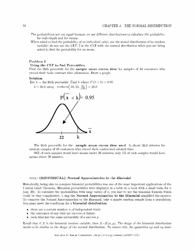
52 CHAPTER 3. THE NORMAL DISTRIBUTION
The probabilities are not equal because we use di�erent distributions to calculate the probabilityfor individuals and for means.
When asked to �nd the probability of an individual value, use the stated distribution of its randomvariable; do not use the CLT. Use the CLT with the normal distribution when you are beingasked to �nd the probability for an mean.
Problem 2Using the CLT to �nd Percentiles:Find the 95th percentile for the sample mean excess time for samples of 80 customers whoexceed their basic contract time allowances. Draw a graph.
SolutionLet k = the 95th percentile. Find k where P (x < k) = 0.95k = 26.0 using invNorm
(.95, 22, 22√
80
)= 26.0
The 95th percentile for the sample mean excess time used is about 26.0 minutes forrandom samples of 80 customers who exceed their contractual allowed time.
95% of such samples would have means under 26 minutes; only 5% of such samples would havemeans above 26 minutes.
note: (HISTORICAL): Normal Approximation to the Binomial
Historically, being able to compute binomial probabilities was one of the most important applications of theCentral Limit Theorem. Binomial probabilities were displayed in a table in a book with a small value for n(say, 20). To calculate the probabilities with large values of n, you had to use the binomial formula whichcould be very complicated. Using the Normal Approximation to the Binomial simpli�ed the process.To compute the Normal Approximation to the Binomial, take a simple random sample from a population.You must meet the conditions for a binomial distribution:
�. there are a certain number n of independent trials�. the outcomes of any trial are success or failure�. each trial has the same probability of a success p
Recall that if X is the binomial random variable, then X∼B (n, p). The shape of the binomial distributionneeds to be similar to the shape of the normal distribution. To ensure this, the quantities np and nq must
Available for free at Connexions <http://cnx.org/content/col10874/1.5>

53
both be greater than �ve (np > 5 and nq > 5; the approximation is better if they are both greater than orequal to 10). Then the binomial can be approximated by the normal distribution with mean µ = np andstandard deviation σ =
√npq. Remember that q = 1 − p. In order to get the best approximation, add 0.5
to x or subtract 0.5 from x (use x + 0.5 or x − 0.5. The number 0.5 is called the continuity correctionfactor.
Example 3.11Suppose in a local Kindergarten through 12th grade (K - 12) school district, 53 percent of thepopulation favor a charter school for grades K - 5. A simple random sample of 300 is surveyed.
1. Find the probability that at least 150 favor a charter school.2. Find the probability that at most 160 favor a charter school.3. Find the probability that more than 155 favor a charter school.4. Find the probability that less than 147 favor a charter school.5. Find the probability that exactly 175 favor a charter school.
Let X = the number that favor a charter school for grades K - 5. X∼B (n, p) where n = 300 andp = 0.53. Since np > 5 and nq > 5, use the normal approximation to the binomial. The formulasfor the mean and standard deviation are µ = np and σ =
√npq. The mean is 159 and the standard
deviation is 8.6447. The random variable for the normal distribution is Y . Y ∼ N (159, 8.6447).See The Normal Distribution for help with calculator instructions.
For Problem 1., you include 150 so P (x ≥ 150) has normal approximation P (Y ≥ 149.5) =0.8641.
normalcdf (149.5, 10^99, 159, 8.6447) = 0.8641.For Problem 2., you include 160 so P (x ≤ 160) has normal approximation P (Y ≤ 160.5) =
0.5689.normalcdf (0, 160.5, 159, 8.6447) = 0.5689For Problem 3., you exclude 155 so P (x > 155) has normal approximation P (y > 155.5) =
0.6572.normalcdf (155.5, 10^99, 159, 8.6447) = 0.6572For Problem 4., you exclude 147 so P (x < 147) has normal approximation P (Y < 146.5) =
0.0741.normalcdf (0, 146.5, 159, 8.6447) = 0.0741For Problem 5., P (x = 175) has normal approximation P (174.5 < y < 175.5) = 0.0083.normalcdf (174.5, 175.5, 159, 8.6447) = 0.0083Because of calculators and computer software that easily let you calculate binomial
probabilities for large values of n, it is not necessary to use the the Normal Approximation tothe Binomial provided you have access to these technology tools. Most school labs have MicrosoftExcel, an example of computer software that calculates binomial probabilities. Many students haveaccess to the TI-83 or 84 series calculators and they easily calculate probabilities for the binomial.In an Internet browser, if you type in "binomial probability distribution calculation," you can �ndat least one online calculator for the binomial.
For Example 3, the probabilities are calculated using the binomial (n = 300 and p = 0.53)below. Compare the binomial and normal distribution answers. SeeDiscrete Random Variablesfor help with calculator instructions for the binomial.
P (x ≥ 150): 1 - binomialcdf (300, 0.53, 149) = 0.8641P (x ≤ 160): binomialcdf (300, 0.53, 160) = 0.5684P (x > 155): 1 - binomialcdf (300, 0.53, 155) = 0.6576P (x < 147): binomialcdf (300, 0.53, 146) = 0.0742P (x = 175): (You use the binomial pdf.) binomialpdf (175, 0.53, 146) = 0.0083
**Contributions made to Example 2 by Roberta Bloom
Available for free at Connexions <http://cnx.org/content/col10874/1.5>

54 CHAPTER 3. THE NORMAL DISTRIBUTION
Solutions to Exercises in Chapter 3
Solution to Example 3.2, Problem 1 (p. 41)This z-score tells you that x = 10 is 2.5 standard deviations to the right of the mean 5.Solution to Example 3.2, Problem 2 (p. 41)z = -4. This z-score tells you that x = −3 is 4 standard deviations to the left of the mean.
Available for free at Connexions <http://cnx.org/content/col10874/1.5>

Chapter 4
Con�dence Interval
4.1 Con�dence Intervals: Introduction1
4.1.1 Student Learning Outcomes
By the end of this chapter, the student should be able to:
• Calculate and interpret con�dence intervals for one population mean and one population proportion.• Interpret the student-t probability distribution as the sample size changes.• Discriminate between problems applying the normal and the student-t distributions.
4.1.2 Introduction
Suppose you are trying to determine the mean rent of a two-bedroom apartment in your town. You mightlook in the classi�ed section of the newspaper, write down several rents listed, and average them together.You would have obtained a point estimate of the true mean. If you are trying to determine the percent oftimes you make a basket when shooting a basketball, you might count the number of shots you make anddivide that by the number of shots you attempted. In this case, you would have obtained a point estimatefor the true proportion.
We use sample data to make generalizations about an unknown population. This part of statistics is calledinferential statistics. The sample data help us to make an estimate of a population parameter.We realize that the point estimate is most likely not the exact value of the population parameter, but closeto it. After calculating point estimates, we construct con�dence intervals in which we believe the parameterlies.
In this chapter, you will learn to construct and interpret con�dence intervals. You will also learn a newdistribution, the Student's-t, and how it is used with these intervals. Throughout the chapter, it is importantto keep in mind that the con�dence interval is a random variable. It is the parameter that is �xed.
If you worked in the marketing department of an entertainment company, you might be interested inthe mean number of compact discs (CD's) a consumer buys per month. If so, you could conduct a surveyand calculate the sample mean, x, and the sample standard deviation, s. You would use x to estimate thepopulation mean and s to estimate the population standard deviation. The sample mean, x, is the pointestimate for the population mean, µ. The sample standard deviation, s, is the point estimate for thepopulation standard deviation, σ.
Each of x and s is also called a statistic.
1This content is available online at <http://cnx.org/content/m16967/1.16/>.
Available for free at Connexions <http://cnx.org/content/col10874/1.5>
55

56 CHAPTER 4. CONFIDENCE INTERVAL
A con�dence interval is another type of estimate but, instead of being just one number, it is an intervalof numbers. The interval of numbers is a range of values calculated from a given set of sample data. Thecon�dence interval is likely to include an unknown population parameter.
Suppose for the CD example we do not know the population mean µ but we do know that the populationstandard deviation is σ = 1 and our sample size is 100. Then by the Central Limit Theorem, the standarddeviation for the sample mean is
σ√n
= 1√100
= 0.1.The Empirical Rule, which applies to bell-shaped distributions, says that in approximately 95% of the
samples, the sample mean, x, will be within two standard deviations of the population mean µ. For our CDexample, two standard deviations is (2) (0.1) = 0.2. The sample mean x is likely to be within 0.2 units ofµ.
Because x is within 0.2 units of µ, which is unknown, then µ is likely to be within 0.2 units of x in 95% ofthe samples. The population mean µ is contained in an interval whose lower number is calculated by takingthe sample mean and subtracting two standard deviations ((2) (0.1)) and whose upper number is calculatedby taking the sample mean and adding two standard deviations. In other words, µ is between x − 0.2 andx+ 0.2 in 95% of all the samples.
For the CD example, suppose that a sample produced a sample mean x = 2. Then the unknownpopulation mean µ is between
x− 0.2 = 2− 0.2 = 1.8 and x+ 0.2 = 2 + 0.2 = 2.2We say that we are 95% con�dent that the unknown population mean number of CDs is between 1.8
and 2.2. The 95% con�dence interval is (1.8, 2.2).The 95% con�dence interval implies two possibilities. Either the interval (1.8, 2.2) contains the true
mean µ or our sample produced an x that is not within 0.2 units of the true mean µ. The second possibilityhappens for only 5% of all the samples (100% - 95%).
Remember that a con�dence interval is created for an unknown population parameter like the populationmean, µ. Con�dence intervals for some parameters have the form
(point estimate - margin of error, point estimate + margin of error)The margin of error depends on the con�dence level or percentage of con�dence.When you read newspapers and journals, some reports will use the phrase "margin of error." Other
reports will not use that phrase, but include a con�dence interval as the point estimate + or - the margin oferror. These are two ways of expressing the same concept.
note: Although the text only covers symmetric con�dence intervals, there are non-symmetriccon�dence intervals (for example, a con�dence interval for the standard deviation).
4.1.3 Optional Collaborative Classroom Activity
Have your instructor record the number of meals each student in your class eats out in a week. Assume thatthe standard deviation is known to be 3 meals. Construct an approximate 95% con�dence interval for thetrue mean number of meals students eat out each week.
1. Calculate the sample mean.2. σ = 3 and n = the number of students surveyed.
3. Construct the interval(x− 2 · σ√
n, x+ 2 · σ√
n
)We say we are approximately 95% con�dent that the true average number of meals that students eat out ina week is between __________ and ___________.
Available for free at Connexions <http://cnx.org/content/col10874/1.5>

57
4.2 Con�dence Intervals: Con�dence Interval, Single Population
Mean, Population Standard Deviation Known, Normal2
4.2.1 Calculating the Con�dence Interval
To construct a con�dence interval for a single unknown population mean µ , where the populationstandard deviation is known, we need x as an estimate for µ and we need the margin of error. Here,the margin of error is called the error bound for a population mean (abbreviated EBM). The samplemean x is the point estimate of the unknown population mean µ
The con�dence interval estimate will have the form:
(point estimate - error bound, point estimate + error bound) or, in symbols,(x− EBM, x+ EBM)
The margin of error depends on the con�dence level (abbreviated CL). The con�dence level is oftenconsidered the probability that the calculated con�dence interval estimate will contain the true populationparameter. However, it is more accurate to state that the con�dence level is the percent of con�denceintervals that contain the true population parameter when repeated samples are taken. Most often, it isthe choice of the person constructing the con�dence interval to choose a con�dence level of 90% or higherbecause that person wants to be reasonably certain of his or her conclusions.
There is another probability called alpha (α). α is related to the con�dence level CL. α is the probabilitythat the interval does not contain the unknown population parameter.Mathematically, α + CL = 1.
Example 4.1
Suppose we have collected data from a sample. We know the sample mean but we do not knowthe mean for the entire population.
The sample mean is 7 and the error bound for the mean is 2.5.
x = 7 and EBM = 2.5.The con�dence interval is (7− 2.5, 7 + 2.5); calculating the values gives (4.5, 9.5).If the con�dence level (CL) is 95%, then we say that "We estimate with 95% con�dence that
the true value of the population mean is between 4.5 and 9.5."
A con�dence interval for a population mean with a known standard deviation is based on the fact that thesample means follow an approximately normal distribution. Suppose that our sample has a mean of x = 10and we have constructed the 90% con�dence interval (5, 15) where EBM = 5.
To get a 90% con�dence interval, we must include the central 90% of the probability of the normaldistribution. If we include the central 90%, we leave out a total of α = 10% in both tails, or 5% in each tail,of the normal distribution.
2This content is available online at <http://cnx.org/content/m16962/1.23/>.
Available for free at Connexions <http://cnx.org/content/col10874/1.5>

58 CHAPTER 4. CONFIDENCE INTERVAL
To capture the central 90%, we must go out 1.645 "standard deviations" on either side of the calculatedsample mean. 1.645 is the z-score from a Standard Normal probability distribution that puts an area of 0.90in the center, an area of 0.05 in the far left tail, and an area of 0.05 in the far right tail.
It is important that the "standard deviation" used must be appropriate for the parameter we are esti-mating. So in this section, we need to use the standard deviation that applies to sample means, which isσ√n. σ√
nis commonly called the "standard error of the mean" in order to clearly distinguish the standard
deviation for a mean from the population standard deviation σ.
In summary, as a result of the Central Limit Theorem:
• X is normally distributed, that is, X ∼ N(µX ,
σ√n
).
• When the population standard deviation σ is known, we use a Normal distribution tocalculate the error bound.
Calculating the Con�dence Interval:To construct a con�dence interval estimate for an unknown population mean, we need data from a randomsample. The steps to construct and interpret the con�dence interval are:
• Calculate the sample mean x from the sample data. Remember, in this section, we already know thepopulation standard deviation σ.
• Find the Z-score that corresponds to the con�dence level.• Calculate the error bound EBM• Construct the con�dence interval• Write a sentence that interprets the estimate in the context of the situation in the problem. (Explain
what the con�dence interval means, in the words of the problem.)
We will �rst examine each step in more detail, and then illustrate the process with some examples.Finding z for the stated Con�dence LevelWhen we know the population standard deviation σ, we use a standard normal distribution to calculate theerror bound EBM and construct the con�dence interval. We need to �nd the value of z that puts an areaequal to the con�dence level (in decimal form) in the middle of the standard normal distribution Z∼N(0,1).
The con�dence level, CL, is the area in the middle of the standard normal distribution. CL = 1− α. Soα is the area that is split equally between the two tails. Each of the tails contains an area equal to α
2 .The z-score that has an area to the right of α2 is denoted by zα
2
For example, when CL = 0.95 then α = 0.05 and α2 = 0.025 ; we write zα
2= z.025
The area to the right of z.025 is 0.025 and the area to the left of z.025 is 1-0.025 = 0.975zα
2= z0.025 = 1.96 , using a calculator, computer or a Standard Normal probability table.
Using the TI83, TI83+ or TI84+ calculator: invNorm(0.975, 0, 1) = 1.96
Available for free at Connexions <http://cnx.org/content/col10874/1.5>
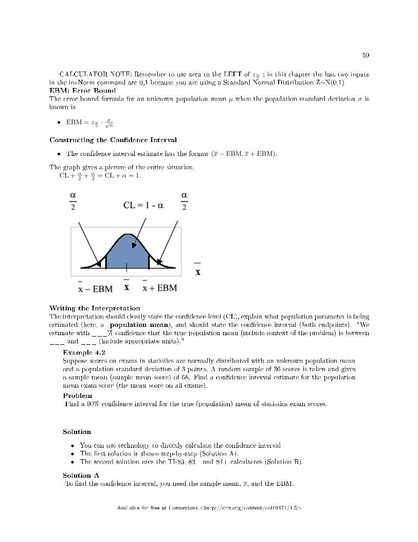
59
CALCULATOR NOTE: Remember to use area to the LEFT of zα2; in this chapter the last two inputs
in the invNorm command are 0,1 because you are using a Standard Normal Distribution Z∼N(0,1)EBM: Error BoundThe error bound formula for an unknown population mean µ when the population standard deviation σ isknown is
• EBM = zα2· σ√
n
Constructing the Con�dence Interval
• The con�dence interval estimate has the format (x− EBM, x+ EBM).
The graph gives a picture of the entire situation.CL + α
2 + α2 = CL + α = 1.
Writing the InterpretationThe interpretation should clearly state the con�dence level (CL), explain what population parameter is beingestimated (here, a population mean), and should state the con�dence interval (both endpoints). "Weestimate with ___% con�dence that the true population mean (include context of the problem) is between___ and ___ (include appropriate units)."
Example 4.2Suppose scores on exams in statistics are normally distributed with an unknown population meanand a population standard deviation of 3 points. A random sample of 36 scores is taken and givesa sample mean (sample mean score) of 68. Find a con�dence interval estimate for the populationmean exam score (the mean score on all exams).
ProblemFind a 90% con�dence interval for the true (population) mean of statistics exam scores.
Solution
• You can use technology to directly calculate the con�dence interval• The �rst solution is shown step-by-step (Solution A).• The second solution uses the TI-83, 83+ and 84+ calculators (Solution B).
Solution ATo �nd the con�dence interval, you need the sample mean, x, and the EBM.
Available for free at Connexions <http://cnx.org/content/col10874/1.5>

60 CHAPTER 4. CONFIDENCE INTERVAL
x = 68EBM = zα
2·(σ√n
)σ = 3 ; n = 36 ; The con�dence level is 90% (CL=0.90)
CL = 0.90 so α = 1− CL = 1− 0.90 = 0.10α2 = 0.05 zα
2= z.05
The area to the right of z.05 is 0.05 and the area to the left of z.05 is 1−0.05=0.95zα
2= z.05 = 1.645
using invNorm(0.95,0,1) on the TI-83,83+,84+ calculators. This can also be found using ap-propriate commands on other calculators, using a computer, or using a probability table for theStandard Normal distribution.
EBM = 1.645 ·(
3√36
)= 0.8225
x− EBM = 68− 0.8225 = 67.1775x+ EBM = 68 + 0.8225 = 68.8225The 90% con�dence interval is (67.1775, 68.8225).
Solution BUsing a function of the TI-83, TI-83+ or TI-84 calculators:
Press STAT and arrow over to TESTS.Arrow down to 7:ZInterval.Press ENTER.Arrow to Stats and press ENTER.Arrow down and enter 3 for σ, 68 for x , 36 for n, and .90 for C-level.Arrow down to Calculate and press ENTER.The con�dence interval is (to 3 decimal places) (67.178, 68.822).InterpretationWe estimate with 90% con�dence that the true population mean exam score for all statistics studentsis between 67.18 and 68.82.Explanation of 90% Con�dence Level90% of all con�dence intervals constructed in this way contain the true mean statistics exam score.For example, if we constructed 100 of these con�dence intervals, we would expect 90 of them tocontain the true population mean exam score.
4.2.2 Changing the Con�dence Level or Sample Size
Example 4.3: Changing the Con�dence LevelSuppose we change the original problem by using a 95% con�dence level. Find a 95% con�denceinterval for the true (population) mean statistics exam score.
SolutionTo �nd the con�dence interval, you need the sample mean, x, and the EBM.
x = 68EBM = zα
2·(σ√n
)σ = 3 ; n = 36 ; The con�dence level is 95% (CL=0.95)
CL = 0.95 so α = 1− CL = 1− 0.95 = 0.05α2 = 0.025 zα
2= z.025
The area to the right of z.025 is 0.025 and the area to the left of z.025 is 1−0.025=0.975
Available for free at Connexions <http://cnx.org/content/col10874/1.5>

61
zα2
= z.025 = 1.96using invnorm(.975,0,1) on the TI-83,83+,84+ calculators. (This can also be found using ap-
propriate commands on other calculators, using a computer, or using a probability table for theStandard Normal distribution.)
EBM = 1.96 ·(
3√36
)= 0.98
x− EBM = 68− 0.98 = 67.02x+ EBM = 68 + 0.98 = 68.98
InterpretationWe estimate with 95 % con�dence that the true population mean for all statistics exam scores isbetween 67.02 and 68.98.Explanation of 95% Con�dence Level95% of all con�dence intervals constructed in this way contain the true value of the populationmean statistics exam score.Comparing the resultsThe 90% con�dence interval is (67.18, 68.82). The 95% con�dence interval is (67.02, 68.98). The95% con�dence interval is wider. If you look at the graphs, because the area 0.95 is larger than thearea 0.90, it makes sense that the 95% con�dence interval is wider.
(a) (b)
Figure 4.1
Summary: E�ect of Changing the Con�dence Level
• Increasing the con�dence level increases the error bound, making the con�dence interval wider.• Decreasing the con�dence level decreases the error bound, making the con�dence interval
narrower.
Example 4.4: Changing the Sample Size:Suppose we change the original problem to see what happens to the error bound if the sample sizeis changed.
ProblemLeave everything the same except the sample size. Use the original 90% con�dence level. Whathappens to the error bound and the con�dence interval if we increase the sample size and use n=100instead of n=36? What happens if we decrease the sample size to n=25 instead of n=36?
� x = 68� EBM = zα
2·(σ√n
)Available for free at Connexions <http://cnx.org/content/col10874/1.5>
62 CHAPTER 4. CONFIDENCE INTERVAL
� σ = 3 ; The con�dence level is 90% (CL=0.90) ; zα2
= z.05 = 1.645
Solution AIf we increase the sample size n to 100, we decrease the error bound.
When n = 100 : EBM = zα2·(σ√n
)= 1.645 ·
(3√100
)= 0.4935
Solution BIf we decrease the sample size n to 25, we increase the error bound.
When n = 25 : EBM = zα2·(σ√n
)= 1.645 ·
(3√25
)= 0.987
Summary: E�ect of Changing the Sample Size
• Increasing the sample size causes the error bound to decrease, making the con�dence intervalnarrower.
• Decreasing the sample size causes the error bound to increase, making the con�dence intervalwider.
4.2.3 Working Backwards to Find the Error Bound or Sample Mean
Working Bacwards to �nd the Error Bound or the Sample MeanWhen we calculate a con�dence interval, we �nd the sample mean and calculate the error bound and usethem to calculate the con�dence interval. But sometimes when we read statistical studies, the study maystate the con�dence interval only. If we know the con�dence interval, we can work backwards to �nd boththe error bound and the sample mean.
Finding the Error Bound
• From the upper value for the interval, subtract the sample mean• OR, From the upper value for the interval, subtract the lower value. Then divide the di�erence by 2.
Finding the Sample Mean
• Subtract the error bound from the upper value of the con�dence interval• OR, Average the upper and lower endpoints of the con�dence interval
Notice that there are two methods to perform each calculation. You can choose the method that is easier touse with the information you know.
Example 4.5Suppose we know that a con�dence interval is (67.18, 68.82) and we want to �nd the error bound.We may know that the sample mean is 68. Or perhaps our source only gave the con�dence intervaland did not tell us the value of the the sample mean.
Calculate the Error Bound:
• If we know that the sample mean is 68: EBM = 68.82− 68 = 0.82• If we don't know the sample mean: EBM = (68.82−67.18)
2 = 0.82
Calculate the Sample Mean:
• If we know the error bound: x = 68.82− 0.82 = 68• If we don't know the error bound: x = (67.18+68.82)
2 = 68
Available for free at Connexions <http://cnx.org/content/col10874/1.5>

63
4.2.4 Calculating the Sample Size n
If researchers desire a speci�c margin of error, then they can use the error bound formula to calculate therequired sample size.
The error bound formula for a population mean when the population standard deviation is known is
EBM = zα2·(σ√n
)The formula for sample size is n = z2σ2
EBM2 , found by solving the error bound formula for nIn this formula, z is zα
2, corresponding to the desired con�dence level. A researcher planning a study who
wants a speci�ed con�dence level and error bound can use this formula to calculate the size of the sampleneeded for the study.
Example 4.6The population standard deviation for the age of Foothill College students is 15 years. If wewant to be 95% con�dent that the sample mean age is within 2 years of the true population meanage of Foothill College students , how many randomly selected Foothill College students must besurveyed?
From the problem, we know that σ = 15 and EBM=2z = z.025 = 1.96, because the con�dence level is 95%.
n = z2σ2
EBM2 = 1.962152
22 =216.09 using the sample size equation.Use n = 217: Always round the answer UP to the next higher integer to ensure that the sample
size is large enough.
Therefore, 217 Foothill College students should be surveyed in order to be 95% con�dent that weare within 2 years of the true population mean age of Foothill College students.
**With contributions from Roberta Bloom
4.3 Con�dence Intervals: Con�dence Interval, Single Population
Mean, Standard Deviation Unknown, Student's-t3
In practice, we rarely know the population standard deviation. In the past, when the sample size was large,this did not present a problem to statisticians. They used the sample standard deviation s as an estimatefor σ and proceeded as before to calculate a con�dence interval with close enough results. However,statisticians ran into problems when the sample size was small. A small sample size caused inaccuracies inthe con�dence interval.
William S. Gossett (1876-1937) of the Guinness brewery in Dublin, Ireland ran into this problem. Hisexperiments with hops and barley produced very few samples. Just replacing σ with s did not produceaccurate results when he tried to calculate a con�dence interval. He realized that he could not use a normaldistribution for the calculation; he found that the actual distribution depends on the sample size. Thisproblem led him to "discover" what is called the Student's-t distribution. The name comes from the factthat Gosset wrote under the pen name "Student."
Up until the mid 1970s, some statisticians used the normal distribution approximation for large samplesizes and only used the Student's-t distribution for sample sizes of at most 30. With the common use ofgraphing calculators and computers, the practice is to use the Student's-t distribution whenever s is used asan estimate for σ.
If you draw a simple random sample of size n from a population that has approximately a normaldistribution with mean µ and unknown population standard deviation σ and calculate the t-score t = x−µ“
s√n
”3This content is available online at <http://cnx.org/content/m16959/1.24/>.
Available for free at Connexions <http://cnx.org/content/col10874/1.5>

64 CHAPTER 4. CONFIDENCE INTERVAL
, then the t-scores follow a Student's-t distribution with n − 1 degrees of freedom. The t-score hasthe same interpretation as the z-score. It measures how far x is from its mean µ. For each sample size n,there is a di�erent Student's-t distribution.
The degrees of freedom, n − 1, come from the calculation of the sample standard deviation s. InChapter 2, we used n deviations (x− x values) to calculate s. Because the sum of the deviations is 0, wecan �nd the last deviation once we know the other n− 1 deviations. The other n− 1 deviations can changeor vary freely. We call the number n− 1 the degrees of freedom (df).
Properties of the Student's-t Distribution
• The graph for the Student's-t distribution is similar to the Standard Normal curve.• The mean for the Student's-t distribution is 0 and the distribution is symmetric about 0.• The Student's-t distribution has more probability in its tails than the Standard Normal distribution
because the spread of the t distribution is greater than the spread of the Standard Normal. So thegraph of the Student's-t distribution will be thicker in the tails and shorter in the center than thegraph of the Standard Normal distribution.
• The exact shape of the Student's-t distribution depends on the "degrees of freedom". As the degreesof freedom increases, the graph Student's-t distribution becomes more like the graph of the StandardNormal distribution.
• The underlying population of individual observations is assumed to be normally distributed with un-known population mean µ and unknown population standard deviation σ. The size of the underlyingpopulation is generally not relevant unless it is very small. If it is bell shaped (normal) then theassumption is met and doesn't need discussion. Random sampling is assumed but it is a completelyseparate assumption from normality.
Calculators and computers can easily calculate any Student's-t probabilities. The TI-83,83+,84+ have a tcdffunction to �nd the probability for given values of t. The grammar for the tcdf command is tcdf(lower bound,upper bound, degrees of freedom). However for con�dence intervals, we need to use inverse probability to�nd the value of t when we know the probability.
For the TI-84+ you can use the invT command on the DISTRibution menu. The invT command workssimilarly to the invnorm. The invT command requires two inputs: invT(area to the left, degrees offreedom) The output is the t-score that corresponds to the area we speci�ed.
The TI-83 and 83+ do not have the invT command. (The TI-89 has an inverse T command.)A probability table for the Student's-t distribution can also be used. The table gives t-scores that
correspond to the con�dence level (column) and degrees of freedom (row). (The TI-86 does not have aninvT program or command, so if you are using that calculator, you need to use a probability table for theStudent's-t distribution.) When using t-table, note that some tables are formatted to show the con�dencelevel in the column headings, while the column headings in some tables may show only corresponding areain one or both tails.
A Student's-t table (See the Table of Contents 15. Tables) gives t-scores given the degrees of free-dom and the right-tailed probability. The table is very limited. Calculators and computers can easilycalculate any Student's-t probabilities.
The notation for the Student's-t distribution is (using T as the random variable) is
• T ∼ tdf where df = n− 1.• For example, if we have a sample of size n=20 items, then we calculate the degrees of freedom as
df=n−1=20−1=19 and we write the distribution as T ∼ t19
If the population standard deviation is not known, the error bound for a population mean is:
• EBM = tα2·(
s√n
)Available for free at Connexions <http://cnx.org/content/col10874/1.5>

65
• tα2is the t-score with area to the right equal toα2
• use df = n− 1 degrees of freedom• s = sample standard deviation
The format for the con�dence interval is:(x− EBM, x+ EBM).The TI-83, 83+ and 84 calculators have a function that calculates the con�dence interval directly. To
get to it,Press STATArrow over to TESTS.Arrow down to 8:TInterval and press ENTER (or just press 8).
Example 4.7Suppose you do a study of acupuncture to determine how e�ective it is in relieving pain. Youmeasure sensory rates for 15 subjects with the results given below. Use the sample data toconstruct a 95% con�dence interval for the mean sensory rate for the population (assumed normal)from which you took the data.
The solution is shown step-by-step and by using the TI-83, 83+ and 84+ calculators.8.6; 9.4; 7.9; 6.8; 8.3; 7.3; 9.2; 9.6; 8.7; 11.4; 10.3; 5.4; 8.1; 5.5; 6.9
Solution
• You can use technology to directly calculate the con�dence interval.• The �rst solution is step-by-step (Solution A).• The second solution uses the Ti-83+ and Ti-84 calculators (Solution B).
Solution ATo �nd the con�dence interval, you need the sample mean, x, and the EBM.
x = 8.2267 s = 1.6722 n = 15df = 15− 1 = 14CL = 0.95 so α = 1− CL = 1− 0.95 = 0.05α2 = 0.025 tα
2= t.025
The area to the right of t.025 is 0.025 and the area to the left of t.025 is 1−0.025=0.975tα
2= t.025 = 2.14 using invT(.975,14) on the TI-84+ calculator.
EBM = tα2·(
s√n
)EBM = 2.14 ·
(1.6722√
15
)= 0.924
x− EBM = 8.2267− 0.9240 = 7.3x+ EBM = 8.2267 + 0.9240 = 9.15The 95% con�dence interval is (7.30, 9.15).We estimate with 95% con�dence that the true population mean sensory rate is between 7.30
and 9.15.
Solution BUsing a function of the TI-83, TI-83+ or TI-84 calculators:
Press STAT and arrow over to TESTS.Arrow down to 8:TInterval and press ENTER (or you can just press 8). Arrow to Data and pressENTER.Arrow down to List and enter the list name where you put the data.Arrow down to Freq and enter 1.Arrow down to C-level and enter .95
Available for free at Connexions <http://cnx.org/content/col10874/1.5>

66 CHAPTER 4. CONFIDENCE INTERVAL
Arrow down to Calculate and press ENTER.The 95% con�dence interval is (7.3006, 9.1527)
note: When calculating the error bound, a probability table for the Student's-t distribution canalso be used to �nd the value of t. The table gives t-scores that correspond to the con�dence level(column) and degrees of freedom (row); the t-score is found where the row and column intersect inthe table.
**With contributions from Roberta Bloom
4.4 Con�dence Intervals: Con�dence Interval for a Population
Proportion4
During an election year, we see articles in the newspaper that state con�dence intervals in terms ofproportions or percentages. For example, a poll for a particular candidate running for president might showthat the candidate has 40% of the vote within 3 percentage points. Often, election polls are calculated with95% con�dence. So, the pollsters would be 95% con�dent that the true proportion of voters who favored thecandidate would be between 0.37 and 0.43 : (0.40− 0.03, 0.40 + 0.03).
Investors in the stock market are interested in the true proportion of stocks that go up and down eachweek. Businesses that sell personal computers are interested in the proportion of households in the UnitedStates that own personal computers. Con�dence intervals can be calculated for the true proportion of stocksthat go up or down each week and for the true proportion of households in the United States that ownpersonal computers.
The procedure to �nd the con�dence interval, the sample size, the error bound, and the con�dencelevel for a proportion is similar to that for the population mean. The formulas are di�erent.
How do you know you are dealing with a proportion problem? First, the underlying distribu-tion is binomial. (There is no mention of a mean or average.) If X is a binomial random variable, thenX ∼ B (n, p) where n = the number of trials and p = the probability of a success. To form a proportion,take X, the random variable for the number of successes and divide it by n, the number of trials (or thesample size). The random variable P ' (read "P prime") is that proportion,
P ' = Xn
(Sometimes the random variable is denoted as P̂ , read "P hat".)When n is large and p is not close to 0 or 1, we can use the normal distribution to approximate the
binomial.X ∼ N
(n · p,√n · p · q
)If we divide the random variable by n, the mean by n, and the standard deviation by n, we get a normal
distribution of proportions with P ', called the estimated proportion, as the random variable. (Recall that aproportion = the number of successes divided by n.)
Xn = P ' ∼ N
(n·pn ,√n·p·qn
)Using algebra to simplify :
√n·p·qn =
√p·qn
P ' follows a normal distribution for proportions: P ' ∼ N(p,√
p·qn
)The con�dence interval has the form (p'−EBP, p'+EBP).p' = x
np' = the estimated proportion of successes (p' is a point estimate for p, the true proportion)x = the number of successes.n = the size of the sample
4This content is available online at <http://cnx.org/content/m16963/1.20/>.
Available for free at Connexions <http://cnx.org/content/col10874/1.5>

67
The error bound for a proportion is
EBP = zα2·√
p'·q'n whereq' = 1− p'
This formula is similar to the error bound formula for a mean, except that the "appropriate standarddeviation" is di�erent. For a mean, when the population standard deviation is known, the appropriate
standard deviation that we use is σ√n. For a proportion, the appropriate standard deviation is
√p·qn .
However, in the error bound formula, we use√
p'·q'n as the standard deviation, instead of
√p·qn
However, in the error bound formula, the standard deviation is√
p'·q'n .
In the error bound formula, the sample proportions p' and q' are estimates of the unknownpopulation proportions p and q. The estimated proportions p' and q' are used because p and q are notknown. p' and q' are calculated from the data. p' is the estimated proportion of successes. q' is the estimatedproportion of failures.
The con�dence interval can only be used if the number of successes np' and the number of failures nq'are both larger than 5.
note: For the normal distribution of proportions, the z-score formula is as follows.
If P ' ∼ N(p,√
p·qn
)then the z-score formula is z = p'−p√
p·qn
Example 4.8Suppose that a market research �rm is hired to estimate the percent of adults living in a largecity who have cell phones. 500 randomly selected adult residents in this city are surveyed todetermine whether they have cell phones. Of the 500 people surveyed, 421 responded yes - theyown cell phones. Using a 95% con�dence level, compute a con�dence interval estimate for the trueproportion of adults residents of this city who have cell phones.
Solution
• You can use technology to directly calculate the con�dence interval.• The �rst solution is step-by-step (Solution A).• The second solution uses a function of the TI-83, 83+ or 84 calculators (Solution B).
Solution ALetX = the number of people in the sample who have cell phones. X is binomial. X ∼ B
(500, 421
500
).
To calculate the con�dence interval, you must �nd p', q', and EBP.n = 500 x = the number of successes = 421p' = x
n = 421500 = 0.842
p' = 0.842 is the sample proportion; this is the point estimate of the population proportion.q' = 1− p' = 1− 0.842 = 0.158Since CL = 0.95, then α = 1− CL = 1− 0.95 = 0.05 α
2 = 0.025.Then zα
2= z.025 = 1.96
Use the TI-83, 83+ or 84+ calculator command invNorm(0.975,0,1) to �nd z.025. Rememberthat the area to the right of z.025 is 0.025 and the area to the left of z0.025 is 0.975. This can alsobe found using appropriate commands on other calculators, using a computer, or using a StandardNormal probability table.
EBP = zα2·√
p'·q'n = 1.96 ·
√(0.842)·(0.158)
500 = 0.032p'− EBP = 0.842− 0.032 = 0.81p' + EBP = 0.842 + 0.032 = 0.874The con�dence interval for the true binomial population proportion is
(p'− EBP, p' + EBP) =(0.810, 0.874).
Available for free at Connexions <http://cnx.org/content/col10874/1.5>

68 CHAPTER 4. CONFIDENCE INTERVAL
InterpretationWe estimate with 95% con�dence that between 81% and 87.4% of all adult residents of this cityhave cell phones.Explanation of 95% Con�dence Level95% of the con�dence intervals constructed in this way would contain the true value for thepopulation proportion of all adult residents of this city who have cell phones.
Solution BUsing a function of the TI-83, 83+ or 84 calculators:
Press STAT and arrow over to TESTS.Arrow down to A:1-PropZint. Press ENTER.Arrow down to x and enter 421.Arrow down to n and enter 500.Arrow down to C-Level and enter .95.Arrow down to Calculate and press ENTER.The con�dence interval is (0.81003, 0.87397).
Example 4.9For a class project, a political science student at a large university wants to estimate the percentof students that are registered voters. He surveys 500 students and �nds that 300 are registeredvoters. Compute a 90% con�dence interval for the true percent of students that are registeredvoters and interpret the con�dence interval.
Solution
• You can use technology to directly calculate the con�dence interval.• The �rst solution is step-by-step (Solution A).• The second solution uses a function of the TI-83, 83+ or 84 calculators (Solution B).
Solution Ax = 300 and n = 500.
p' = xn = 300
500 = 0.600q' = 1− p' = 1− 0.600 = 0.400Since CL = 0.90, then α = 1− CL = 1− 0.90 = 0.10 α
2 = 0.05.zα
2= z.05 = 1.645
Use the TI-83, 83+ or 84+ calculator command invNorm(0.95,0,1) to �nd z.05. Remember thatthe area to the right of z.05 is 0.05 and the area to the left of z.05 is 0.95. This can also be foundusing appropriate commands on other calculators, using a computer, or using a Standard Normalprobability table.
EBP = zα2·√
p'·q'n = 1.645 ·
√(0.60)·(0.40)
500 = 0.036p'− EBP = 0.60− 0.036 = 0.564
p' + EBP = 0.60 + 0.036 = 0.636The con�dence interval for the true binomial population proportion is
(p'− EBP, p' + EBP) =(0.564, 0.636).Interpretation:
Available for free at Connexions <http://cnx.org/content/col10874/1.5>
69
• We estimate with 90% con�dence that the true percent of all students that are registeredvoters is between 56.4% and 63.6%.
• Alternate Wording: We estimate with 90% con�dence that between 56.4% and 63.6% of ALLstudents are registered voters.
Explanation of 90% Con�dence Level90% of all con�dence intervals constructed in this way contain the true value for the populationpercent of students that are registered voters.
Solution BUsing a function of the TI-83, 83+ or 84 calculators:
Press STAT and arrow over to TESTS.Arrow down to A:1-PropZint. Press ENTER.Arrow down to x and enter 300.Arrow down to n and enter 500.Arrow down to C-Level and enter .90.Arrow down to Calculate and press ENTER.The con�dence interval is (0.564, 0.636).
4.4.1 Calculating the Sample Size n
If researchers desire a speci�c margin of error, then they can use the error bound formula to calculate therequired sample size.
The error bound formula for a population proportion is
• EBP = zα2·√
p'q'n
• Solving for n gives you an equation for the sample size.
• n =zα
22·p'q'
EBP2
Example 4.10Suppose a mobile phone company wants to determine the current percentage of customers aged50+ that use text messaging on their cell phone. How many customers aged 50+ should thecompany survey in order to be 90% con�dent that the estimated (sample) proportion is within 3percentage points of the true population proportion of customers aged 50+ that use text messagingon their cell phone.
SolutionFrom the problem, we know that EBP=0.03 (3%=0.03) and
zα2
= z.05 = 1.645 because the con�dence level is 90%However, in order to �nd n , we need to know the estimated (sample) proportion p'. Remember
that q'=1-p'. But, we do not know p' yet. Since we multiply p' and q' together, we make themboth equal to 0.5 because p'q'= (.5)(.5)=.25 results in the largest possible product. (Try otherproducts: (.6)(.4)=.24; (.3)(.7)=.21; (.2)(.8)=.16 and so on). The largest possible product gives usthe largest n. This gives us a large enough sample so that we can be 90% con�dent that we arewithin 3 percentage points of the true population proportion. To calculate the sample size n, usethe formula and make the substitutions.
n = z2p'q'EBP2 gives n = 1.6452(.5)(.5)
.032 =751.7
Available for free at Connexions <http://cnx.org/content/col10874/1.5>

70 CHAPTER 4. CONFIDENCE INTERVAL
Round the answer to the next higher value. The sample size should be 752 cell phone customersaged 50+ in order to be 90% con�dent that the estimated (sample) proportion is within 3 percentagepoints of the true population proportion of all customers aged 50+ that use text messaging on theircell phone.
**With contributions from Roberta Bloom.
Available for free at Connexions <http://cnx.org/content/col10874/1.5>

Chapter 5
Hypothesis Testing
5.1 Hypothesis Testing of Single Mean and Single Proportion:
Introduction1
5.1.1 Student Learning Outcomes
By the end of this chapter, the student should be able to:
• Di�erentiate between Type I and Type II Errors• Describe hypothesis testing in general and in practice• Conduct and interpret hypothesis tests for a single population mean, population standard deviation
known.• Conduct and interpret hypothesis tests for a single population mean, population standard deviation
unknown.• Conduct and interpret hypothesis tests for a single population proportion.
5.1.2 Introduction
One job of a statistician is to make statistical inferences about populations based on samples taken from thepopulation. Con�dence intervals are one way to estimate a population parameter. Another way to makea statistical inference is to make a decision about a parameter. For instance, a car dealer advertises thatits new small truck gets 35 miles per gallon, on the average. A tutoring service claims that its method oftutoring helps 90% of its students get an A or a B. A company says that women managers in their companyearn an average of $60,000 per year.
A statistician will make a decision about these claims. This process is called "hypothesis testing." Ahypothesis test involves collecting data from a sample and evaluating the data. Then, the statistician makesa decision as to whether or not there is su�cient evidence based upon analyses of the data, to reject the nullhypothesis.
In this chapter, you will conduct hypothesis tests on single means and single proportions. You will alsolearn about the errors associated with these tests.
Hypothesis testing consists of two contradictory hypotheses or statements, a decision based on the data,and a conclusion. To perform a hypothesis test, a statistician will:
1. Set up two contradictory hypotheses.2. Collect sample data (in homework problems, the data or summary statistics will be given to you).3. Determine the correct distribution to perform the hypothesis test.
1This content is available online at <http://cnx.org/content/m16997/1.11/>.
Available for free at Connexions <http://cnx.org/content/col10874/1.5>
71

72 CHAPTER 5. HYPOTHESIS TESTING
4. Analyze sample data by performing the calculations that ultimately will allow you to reject or fail toreject the null hypothesis.
5. Make a decision and write a meaningful conclusion.
note: To do the hypothesis test homework problems for this chapter and later chapters, makecopies of the appropriate special solution sheets. See the Table of Contents topic "Solution Sheets".
5.2 Hypothesis Testing of Single Mean and Single Proportion: Null
and Alternate Hypotheses2
The actual test begins by considering two hypotheses. They are called the null hypothesis and thealternate hypothesis. These hypotheses contain opposing viewpoints.
Ho: The null hypothesis: It is a statement about the population that will be assumed to be trueunless it can be shown to be incorrect beyond a reasonable doubt.
Ha: The alternate hypothesis: It is a claim about the population that is contradictory to Ho andwhat we conclude when we reject Ho.
Example 5.1Ho: No more than 30% of the registered voters in Santa Clara County voted in the primary election.
Ha: More than 30% of the registered voters in Santa Clara County voted in the primary election.
Example 5.2We want to test whether the mean grade point average in American colleges is di�erent from 2.0(out of 4.0).
Ho: µ = 2.0 Ha: µ 6= 2.0
Example 5.3We want to test if college students take less than �ve years to graduate from college, on the average.
Ho: µ ≥ 5 Ha: µ < 5
Example 5.4In an issue of U. S. News and World Report, an article on school standards stated that abouthalf of all students in France, Germany, and Israel take advanced placement exams and a thirdpass. The same article stated that 6.6% of U. S. students take advanced placement exams and 4.4% pass. Test if the percentage of U. S. students who take advanced placement exams is more than6.6%.
Ho: p= 0.066 Ha: p > 0.066Since the null and alternate hypotheses are contradictory, you must examine evidence to decide if you haveenough evidence to reject the null hypothesis or not. The evidence is in the form of sample data.
After you have determined which hypothesis the sample supports, you make a decision. There are twooptions for a decision. They are "reject Ho" if the sample information favors the alternate hypothesis or "donot reject Ho" or "fail to reject Ho" if the sample information is insu�cient to reject the null hypothesis.
Mathematical Symbols Used in Ho and Ha:
Ho Ha
equal (=) not equal ( 6=) or greater than (> ) or less than (<)
greater than or equal to (≥) less than (<)
less than or equal to (≤) more than (> )
2This content is available online at <http://cnx.org/content/m16998/1.14/>.
Available for free at Connexions <http://cnx.org/content/col10874/1.5>

73
Table 5.1
note: Ho always has a symbol with an equal in it. Ha never has a symbol with an equal in it.The choice of symbol depends on the wording of the hypothesis test. However, be aware that manyresearchers (including one of the co-authors in research work) use = in the Null Hypothesis, evenwith > or < as the symbol in the Alternate Hypothesis. This practice is acceptable because weonly make the decision to reject or not reject the Null Hypothesis.
5.2.1 Optional Collaborative Classroom Activity
Bring to class a newspaper, some news magazines, and some Internet articles . In groups, �nd articles fromwhich your group can write a null and alternate hypotheses. Discuss your hypotheses with the rest of theclass.
5.3 Hypothesis Testing of Single Mean and Single Proportion: Using
the Sample to Test the Null Hypothesis3
Use the sample data to calculate the actual probability of getting the test result, called the p-value. Thep-value is the probability that, if the null hypothesis is true, the results from another randomlyselected sample will be as extreme or more extreme as the results obtained from the givensample.
A large p-value calculated from the data indicates that we should fail to reject the null hypothesis.The smaller the p-value, the more unlikely the outcome, and the stronger the evidence is against the nullhypothesis. We would reject the null hypothesis if the evidence is strongly against it.
Draw a graph that shows the p-value. The hypothesis test is easier to perform if you use agraph because you see the problem more clearly.
Example 5.5: (to illustrate the p-value)Suppose a baker claims that his bread height is more than 15 cm, on the average. Several of hiscustomers do not believe him. To persuade his customers that he is right, the baker decides to do ahypothesis test. He bakes 10 loaves of bread. The mean height of the sample loaves is 17 cm. Thebaker knows from baking hundreds of loaves of bread that the standard deviation for the heightis 0.5 cm. and the distribution of heights is normal.
The null hypothesis could be Ho: µ ≤ 15 The alternate hypothesis is Ha: µ > 15The words "is more than" translates as a "> " so "µ > 15" goes into the alternate hypothesis.
The null hypothesis must contradict the alternate hypothesis.Since σ is known (σ = 0.5 cm.), the distribution for the population is known to be normal
with mean µ= 15 and standard deviation σ√n
= 0.5√10
= 0.16.Suppose the null hypothesis is true (the mean height of the loaves is no more than 15 cm). Then
is the mean height (17 cm) calculated from the sample unexpectedly large? The hypothesis testworks by asking the question how unlikely the sample mean would be if the null hypothesis weretrue. The graph shows how far out the sample mean is on the normal curve. The p-value is theprobability that, if we were to take other samples, any other sample mean would fall at least as farout as 17 cm.
The p-value, then, is the probability that a sample mean is the same or greater than17 cm. when the population mean is, in fact, 15 cm. We can calculate this probabilityusing the normal distribution for means from Chapter 7.
3This content is available online at <http://cnx.org/content/m16995/1.17/>.
Available for free at Connexions <http://cnx.org/content/col10874/1.5>

74 CHAPTER 5. HYPOTHESIS TESTING
p-value = P (x > 17) which is approximately 0.A p-value of approximately 0 tells us that it is highly unlikely that a loaf of bread rises no more
than 15 cm, on the average. That is, almost 0% of all loaves of bread would be at least as highas 17 cm. purely by CHANCE had the population mean height really been 15 cm. Becausethe outcome of 17 cm. is so unlikely (meaning it is happening NOT by chance alone), weconclude that the evidence is strongly against the null hypothesis (the mean height is at most 15cm.). There is su�cient evidence that the true mean height for the population of the baker's loavesof bread is greater than 15 cm.
5.4 Hypothesis Testing of Single Mean and Single Proportion: Deci-
sion and Conclusion4
A systematic way to make a decision of whether to reject or not reject the null hypothesis is to comparethe p-value and a preset or preconceived α (also called a "signi�cance level"). A preset α is theprobability of a Type I error (rejecting the null hypothesis when the null hypothesis is true). It may ormay not be given to you at the beginning of the problem.
When you make a decision to reject or not reject Ho, do as follows:
• If α > p-value, reject Ho. The results of the sample data are signi�cant. There is su�cient evidenceto conclude that Ho is an incorrect belief and that the alternative hypothesis, Ha, may be correct.
• If α ≤ p-value, do not reject Ho. The results of the sample data are not signi�cant. There is notsu�cient evidence to conclude that the alternative hypothesis, Ha, may be correct.
• When you "do not reject Ho", it does not mean that you should believe that Ho is true. It simplymeans that the sample data have failed to provide su�cient evidence to cast serious doubt about thetruthfulness of Ho.
Conclusion: After you make your decision, write a thoughtful conclusion about the hypotheses interms of the given problem.
4This content is available online at <http://cnx.org/content/m16992/1.11/>.
Available for free at Connexions <http://cnx.org/content/col10874/1.5>

Chapter 6
Linear Regression and Correlation
6.1 Linear Regression and Correlation: Introduction1
6.1.1 Student Learning Outcomes
By the end of this chapter, the student should be able to:
• Discuss basic ideas of linear regression and correlation.• Create and interpret a line of best �t.• Calculate and interpret the correlation coe�cient.• Calculate and interpret outliers.
6.1.2 Introduction
Professionals often want to know how two or more numeric variables are related. For example, is there arelationship between the grade on the second math exam a student takes and the grade on the �nal exam?If there is a relationship, what is it and how strong is the relationship?
In another example, your income may be determined by your education, your profession, your years ofexperience, and your ability. The amount you pay a repair person for labor is often determined by an initialamount plus an hourly fee. These are all examples in which regression can be used.
The type of data described in the examples is bivariate data - "bi" for two variables. In reality,statisticians use multivariate data, meaning many variables.
In this chapter, you will be studying the simplest form of regression, "linear regression" with one inde-pendent variable (x). This involves data that �ts a line in two dimensions. You will also study correlationwhich measures how strong the relationship is.
6.2 Linear Regression and Correlation: Linear Equations2
Linear regression for two variables is based on a linear equation with one independent variable. It has theform:
y = a+ bx (6.1)
where a and b are constant numbers.
1This content is available online at <http://cnx.org/content/m17089/1.6/>.2This content is available online at <http://cnx.org/content/m17086/1.4/>.
Available for free at Connexions <http://cnx.org/content/col10874/1.5>
75
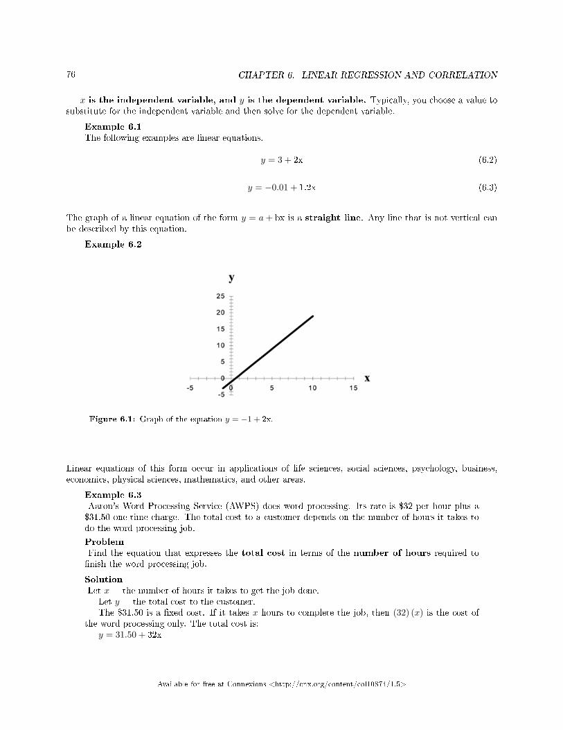
76 CHAPTER 6. LINEAR REGRESSION AND CORRELATION
x is the independent variable, and y is the dependent variable. Typically, you choose a value tosubstitute for the independent variable and then solve for the dependent variable.
Example 6.1The following examples are linear equations.
y = 3 + 2x (6.2)
y = −0.01 + 1.2x (6.3)
The graph of a linear equation of the form y = a+ bx is a straight line. Any line that is not vertical canbe described by this equation.
Example 6.2
Figure 6.1: Graph of the equation y = −1 + 2x.
Linear equations of this form occur in applications of life sciences, social sciences, psychology, business,economics, physical sciences, mathematics, and other areas.
Example 6.3Aaron's Word Processing Service (AWPS) does word processing. Its rate is $32 per hour plus a$31.50 one-time charge. The total cost to a customer depends on the number of hours it takes todo the word processing job.
ProblemFind the equation that expresses the total cost in terms of the number of hours required to�nish the word processing job.
SolutionLet x = the number of hours it takes to get the job done.
Let y = the total cost to the customer.The $31.50 is a �xed cost. If it takes x hours to complete the job, then (32) (x) is the cost of
the word processing only. The total cost is:y = 31.50 + 32x
Available for free at Connexions <http://cnx.org/content/col10874/1.5>

77
6.3 Linear Regression and Correlation: Slope and Y-Intercept of a
Linear Equation3
For the linear equation y = a+ bx, b = slope and a = y-intercept.From algebra recall that the slope is a number that describes the steepness of a line and the y-intercept
is the y coordinate of the point (0, a) where the line crosses the y-axis.
(a) (b) (c)
Figure 6.2: Three possible graphs of y = a + bx. (a) If b > 0, the line slopes upward to the right. (b)If b = 0, the line is horizontal. (c) If b < 0, the line slopes downward to the right.
Example 6.4Svetlana tutors to make extra money for college. For each tutoring session, she charges a one timefee of $25 plus $15 per hour of tutoring. A linear equation that expresses the total amount of moneySvetlana earns for each session she tutors is y = 25 + 15x.
ProblemWhat are the independent and dependent variables? What is the y-intercept and what is theslope? Interpret them using complete sentences.
SolutionThe independent variable (x) is the number of hours Svetlana tutors each session. The dependentvariable (y) is the amount, in dollars, Svetlana earns for each session.
The y-intercept is 25 (a = 25). At the start of the tutoring session, Svetlana charges a one-timefee of $25 (this is when x = 0). The slope is 15 (b = 15). For each session, Svetlana earns $15 foreach hour she tutors.
6.4 Linear Regression and Correlation: Scatter Plots4
Before we take up the discussion of linear regression and correlation, we need to examine a way to displaythe relation between two variables x and y. The most common and easiest way is a scatter plot. Thefollowing example illustrates a scatter plot.
3This content is available online at <http://cnx.org/content/m17083/1.5/>.4This content is available online at <http://cnx.org/content/m17082/1.8/>.
Available for free at Connexions <http://cnx.org/content/col10874/1.5>

78 CHAPTER 6. LINEAR REGRESSION AND CORRELATION
Example 6.5From an article in the Wall Street Journal: In Europe and Asia, m-commerce is popular. M-commerce users have special mobile phones that work like electronic wallets as well as providephone and Internet services. Users can do everything from paying for parking to buying a TV setor soda from a machine to banking to checking sports scores on the Internet. For the years 2000through 2004, was there a relationship between the year and the number of m-commerce users?Construct a scatter plot. Let x = the year and let y = the number of m-commerce users, in millions.
x (year) y (# of users)
2000 0.5
2002 20.0
2003 33.0
2004 47.0(a)
(b)
Figure 6.3: (a) Table showing the number of m-commerce users (in millions) by year. (b) Scatter plotshowing the number of m-commerce users (in millions) by year.
A scatter plot shows the direction and strength of a relationship between the variables. A clear directionhappens when there is either:
• High values of one variable occurring with high values of the other variable or low values of one variableoccurring with low values of the other variable.
• High values of one variable occurring with low values of the other variable.
You can determine the strength of the relationship by looking at the scatter plot and seeing how closethe points are to a line, a power function, an exponential function, or to some other type of function.
When you look at a scatterplot, you want to notice the overall pattern and any deviations from thepattern. The following scatterplot examples illustrate these concepts.
Available for free at Connexions <http://cnx.org/content/col10874/1.5>

79
(a) Positive Linear Pattern (Strong) (b) Linear Pattern w/ One Deviation
Figure 6.4
(a) Negative Linear Pattern (Strong) (b) Negative Linear Pattern (Weak)
Figure 6.5
(a) Exponential Growth Pattern (b) No Pattern
Figure 6.6
In this chapter, we are interested in scatter plots that show a linear pattern. Linear patterns are quitecommon. The linear relationship is strong if the points are close to a straight line. If we think that the pointsshow a linear relationship, we would like to draw a line on the scatter plot. This line can be calculated througha process called linear regression. However, we only calculate a regression line if one of the variables helpsto explain or predict the other variable. If x is the independent variable and y the dependent variable, thenwe can use a regression line to predict y for a given value of x.
Available for free at Connexions <http://cnx.org/content/col10874/1.5>
80 CHAPTER 6. LINEAR REGRESSION AND CORRELATION
6.5 Linear Regression and Correlation: The Regression Equation5
Data rarely �t a straight line exactly. Usually, you must be satis�ed with rough predictions. Typically, youhave a set of data whose scatter plot appears to "�t" a straight line. This is called a Line of Best Fit orLeast Squares Line.
6.5.1 Optional Collaborative Classroom Activity
If you know a person's pinky (smallest) �nger length, do you think you could predict that person's height?Collect data from your class (pinky �nger length, in inches). The independent variable, x, is pinky �ngerlength and the dependent variable, y, is height.
For each set of data, plot the points on graph paper. Make your graph big enough and use a ruler.Then "by eye" draw a line that appears to "�t" the data. For your line, pick two convenient points and usethem to �nd the slope of the line. Find the y-intercept of the line by extending your lines so they cross they-axis. Using the slopes and the y-intercepts, write your equation of "best �t". Do you think everyone willhave the same equation? Why or why not?
Using your equation, what is the predicted height for a pinky length of 2.5 inches?Example 6.6A random sample of 11 statistics students produced the following data where x is the third examscore, out of 80, and y is the �nal exam score, out of 200. Can you predict the �nal exam score ofa random student if you know the third exam score?
5This content is available online at <http://cnx.org/content/m17090/1.15/>.
Available for free at Connexions <http://cnx.org/content/col10874/1.5>

81
x (third exam score) y (�nal exam score)
65 175
67 133
71 185
71 163
66 126
75 198
67 153
70 163
71 159
69 151
69 159(a)
(b)
Figure 6.7: (a) Table showing the scores on the �nal exam based on scores from the third exam. (b)Scatter plot showing the scores on the �nal exam based on scores from the third exam.
The third exam score, x, is the independent variable and the �nal exam score, y, is the dependent variable.We will plot a regression line that best "�ts" the data. If each of you were to �t a line "by eye", you woulddraw di�erent lines. We can use what is called a least-squares regression line to obtain the best �t line.
Consider the following diagram. Each point of data is of the the form (x, y)and each point of the line of
best �t using least-squares linear regression has the form
(x,^y
).
The^y is read "y hat" and is the estimated value of y. It is the value of y obtained using the regression
line. It is not generally equal to y from data.
Available for free at Connexions <http://cnx.org/content/col10874/1.5>

82 CHAPTER 6. LINEAR REGRESSION AND CORRELATION
Figure 6.8
The term y0 −^y0 = ε0 is called the "error" or residual. It is not an error in the sense of a mistake.
The absolute value of a residual measures the vertical distance between the actual value of y and theestimated value of y. In other words, it measures the vertical distance between the actual data point andthe predicted point on the line.
If the observed data point lies above the line, the residual is positive, and the line underestimates theactual data value for y. If the observed data point lies below the line, the residual is negative, and the lineoverestimates that actual data value for y.
In the diagram above, y0−^y0 = ε0 is the residual for the point shown. Here the point lies above the line
and the residual is positive.ε = the Greek letter epsilon
For each data point, you can calculate the residuals or errors, yi −^yi = εi for i = 1, 2, 3, ..., 11.
Each |ε| is a vertical distance.For the example about the third exam scores and the �nal exam scores for the 11 statistics students,
there are 11 data points. Therefore, there are 11 ε values. If you square each ε and add, you get
(ε1)2 + (ε2)2 + ... + (ε11)2 =11
Σi = 1
ε2
This is called the Sum of Squared Errors (SSE).Using calculus, you can determine the values of a and b that make the SSE a minimum. When you make
the SSE a minimum, you have determined the points that are on the line of best �t. It turns out that theline of best �t has the equation:
^y= a+ bx (6.4)
where a = y − b · x and b = Σ(x−x)·(y−y)
Σ(x−x)2.
x and y are the sample means of the x values and the y values, respectively. The best �t line alwayspasses through the point (x, y).
The slope b can be written as b = r ·(sysx
)where sy = the standard deviation of the y values and sx =
the standard deviation of the x values. r is the correlation coe�cient which is discussed in the next section.Least Squares Criteria for Best FitThe process of �tting the best �t line is called linear regression. The idea behind �nding the best �t line
Available for free at Connexions <http://cnx.org/content/col10874/1.5>

83
is based on the assumption that the data are scattered about a straight line. The criteria for the best �tline is that the sum of the squared errors (SSE) is minimized, that is made as small as possible. Any otherline you might choose would have a higher SSE than the best �t line. This best �t line is called the leastsquares regression line .
note: Computer spreadsheets, statistical software, and many calculators can quickly calculate thebest �t line and create the graphs. The calculations tend to be tedious if done by hand. Instructionsto use the TI-83, TI-83+, and TI-84+ calculators to �nd the best �t line and create a scatterplotare shown at the end of this section.
THIRD EXAM vs FINAL EXAM EXAMPLE:The graph of the line of best �t for the third exam/�nal exam example is shown below:
Figure 6.9
The least squares regression line (best �t line) for the third exam/�nal exam example has the equation:
^y= −173.51 + 4.83x (6.5)
note:
Remember, it is always important to plot a scatter diagram �rst. If the scatter plot indicates thatthere is a linear relationship between the variables, then it is reasonable to use a best �t lineto make predictions for y given x within the domain of x-values in the sample data, but notnecessarily for x-values outside that domain.
You could use the line to predict the �nal exam score for a student who earned a grade of 73 onthe third exam.
You should NOT use the line to predict the �nal exam score for a student who earned a grade of50 on the third exam, because 50 is not within the domain of the x-values in the sample data,which are between 65 and 75.
Available for free at Connexions <http://cnx.org/content/col10874/1.5>

84 CHAPTER 6. LINEAR REGRESSION AND CORRELATION
UNDERSTANDING SLOPEThe slope of the line, b, describes how changes in the variables are related. It is important to interpretthe slope of the line in the context of the situation represented by the data. You should be able to write asentence interpreting the slope in plain English.
INTERPRETATION OF THE SLOPE: The slope of the best �t line tells us how the dependentvariable (y) changes for every one unit increase in the independent (x) variable, on average.
THIRD EXAM vs FINAL EXAM EXAMPLE
Slope: The slope of the line is b = 4.83.Interpretation: For a one point increase in the score on the third exam, the �nal exam score increases by
4.83 points, on average.
6.5.2 Using the TI-83+ and TI-84+ Calculators
Using the Linear Regression T Test: LinRegTTest
Step 1. In the STAT list editor, enter the X data in list L1 and the Y data in list L2, paired so that thecorresponding (x,y) values are next to each other in the lists. (If a particular pair of values is repeated,enter it as many times as it appears in the data.)
Step 2. On the STAT TESTS menu, scroll down with the cursor to select the LinRegTTest. (Be careful toselect LinRegTTest as some calculators may also have a di�erent item called LinRegTInt.)
Step 3. On the LinRegTTest input screen enter: Xlist: L1 ; Ylist: L2 ; Freq: 1Step 4. On the next line, at the prompt β or ρ, highlight "6= 0" and press ENTERStep 5. Leave the line for "RegEq:" blankStep 6. Highlight Calculate and press ENTER.
Figure 6.10
The output screen contains a lot of information. For now we will focus on a few items from the output,and will return later to the other items.
Available for free at Connexions <http://cnx.org/content/col10874/1.5>

85
The second line says y=a+bx. Scroll down to �nd the values a=-173.513, and b=4.8273 ; the equation of
the best �t line is^y= −173.51 + 4.83x
The two items at the bottom are r2 = .43969 and r=.663. For now, just note where to �nd these values;we will discuss them in the next two sections.
Graphing the Scatterplot and Regression Line
Step 1. We are assuming your X data is already entered in list L1 and your Y data is in list L2Step 2. Press 2nd STATPLOT ENTER to use Plot 1Step 3. On the input screen for PLOT 1, highlight On and press ENTERStep 4. For TYPE: highlight the very �rst icon which is the scatterplot and press ENTERStep 5. Indicate Xlist: L1 and Ylist: L2Step 6. For Mark: it does not matter which symbol you highlight.Step 7. Press the ZOOM key and then the number 9 (for menu item "ZoomStat") ; the calculator will �t the
window to the dataStep 8. To graph the best �t line, press the "Y=" key and type the equation -173.5+4.83X into equation Y1.
(The X key is immediately left of the STAT key). Press ZOOM 9 again to graph it.Step 9. Optional: If you want to change the viewing window, press the WINDOW key. Enter your desired
window using Xmin, Xmax, Ymin, Ymax
**With contributions from Roberta Bloom
6.6 Linear Regression and Correlation: Correlation Coe�cient and
Coe�cient of Determination6
6.6.1 The Correlation Coe�cient r
Besides looking at the scatter plot and seeing that a line seems reasonable, how can you tell if the line is agood predictor? Use the correlation coe�cient as another indicator (besides the scatterplot) of the strengthof the relationship between x and y.
The correlation coe�cient, r, developed by Karl Pearson in the early 1900s, is a numerical measureof the strength of association between the independent variable x and the dependent variable y.
The correlation coe�cient is calculated as
r =n · Σx · y − (Σx) · (Σy)√[
n · Σx2 − (Σx)2]·[n · Σy2 − (Σy)2
] (6.6)
where n = the number of data points.If you suspect a linear relationship between x and y, then r can measure how strong the linear relationship
is.
What the VALUE of r tells us:
• The value of r is always between -1 and +1: −1 ≤ r ≤ 1.• The size of the correlation r indicates the strength of the linear relationship between x and y. Values
of r close to -1 or to +1 indicate a stronger linear relationship between x and y.• If r = 0 there is absolutely no linear relationship between x and y (no linear correlation).• If r = 1, there is perfect positive correlation. If r = −1, there is perfect negative correlation. In both
these cases, all of the original data points lie on a straight line. Of course, in the real world, this willnot generally happen.
6This content is available online at <http://cnx.org/content/m17092/1.12/>.
Available for free at Connexions <http://cnx.org/content/col10874/1.5>

86 CHAPTER 6. LINEAR REGRESSION AND CORRELATION
What the SIGN of r tells us
• A positive value of r means that when x increases, y tends to increase and when x decreases, y tendsto decrease (positive correlation).
• A negative value of r means that when x increases, y tends to decrease and when x decreases, y tendsto increase (negative correlation).
• The sign of r is the same as the sign of the slope, b, of the best �t line.
note: Strong correlation does not suggest that x causes y or y causes x. We say "correlationdoes not imply causation." For example, every person who learned math in the 17th century isdead. However, learning math does not necessarily cause death!
(a) Positive Correlation (b) Negative Correlation
(c) Zero Correlation
Figure 6.11: (a) A scatter plot showing data with a positive correlation. 0 < r < 1 (b) A scatterplot showing data with a negative correlation. −1 < r < 0 (c) A scatter plot showing data with zerocorrelation. r=0
The formula for r looks formidable. However, computer spreadsheets, statistical software, and manycalculators can quickly calculate r. The correlation coe�cient r is the bottom item in the output screens forthe LinRegTTest on the TI-83, TI-83+, or TI-84+ calculator (see previous section for instructions).
6.6.2 The Coe�cient of Determination
r2 is called the coe�cient of determination. r2 is the square of the correlation coe�cient , butis usually stated as a percent, rather than in decimal form. r2 has an interpretation in the context of thedata:
• r2, when expressed as a percent, represents the percent of variation in the dependent variable y thatcan be explained by variation in the independent variable x using the regression (best �t) line.
Available for free at Connexions <http://cnx.org/content/col10874/1.5>

87
• 1-r2, when expressed as a percent, represents the percent of variation in y that is NOT explained byvariation in x using the regression line. This can be seen as the scattering of the observed data pointsabout the regression line.
Consider the third exam/�nal exam example introduced in the previous section
The line of best �t is:^y= −173.51 + 4.83x
The correlation coe�cient is r = 0.6631The coe�cient of determination is r2 = 0.66312 = 0.4397Interpretation of r2 in the context of this example:Approximately 44% of the variation (0.4397 is approximately 0.44) in the �nal exam grades can be explained
by the variation in the grades on the third exam, using the best �t regression line.Therefore approximately 56% of the variation (1 - 0.44 = 0.56) in the �nal exam grades can NOT be
explained by the variation in the grades on the third exam, using the best �t regression line. (This isseen as the scattering of the points about the line.)
**With contributions from Roberta Bloom.
6.7 Linear Regression and Correlation: Testing the Signi�cance of
the Correlation Coe�cient7
6.7.1 Testing the Signi�cance of the Correlation Coe�cient
The correlation coe�cient, r, tells us about the strength of the linear relationship between x and y. However,the reliability of the linear model also depends on how many observed data points are in the sample. Weneed to look at both the value of the correlation coe�cient r and the sample size n, together.
We perform a hypothesis test of the "signi�cance of the correlation coe�cient" to decide whetherthe linear relationship in the sample data is strong enough to use to model the relationship in the population.
The sample data is used to compute r, the correlation coe�cient for the sample. If we had data for theentire population, we could �nd the population correlation coe�cient. But because we only have sampledata, we can not calculate the population correlation coe�cient. The sample correlation coe�cient, r, is ourestimate of the unknown population correlation coe�cient.
The symbol for the population correlation coe�cient is ρ, the Greek letter "rho".ρ = population correlation coe�cient (unknown)r = sample correlation coe�cient (known; calculated from sample data)
The hypothesis test lets us decide whether the value of the population correlation coe�cient ρ is "close to0" or "signi�cantly di�erent from 0". We decide this based on the sample correlation coe�cient r and thesample size n.
If the test concludes that the correlation coe�cient is signi�cantly di�erent from 0, we saythat the correlation coe�cient is "signi�cant".
• Conclusion: "There is su�cient evidence to conclude that there is a signi�cant linear relationshipbetween x and y because the correlation coe�cient is signi�cantly di�erent from 0."
• What the conclusion means: There is a signi�cant linear relationship between x and y. We can usethe regression line to model the linear relationship between x and y in the population.
If the test concludes that the correlation coe�cient is not signi�cantly di�erent from 0 (it isclose to 0), we say that correlation coe�cient is "not signi�cant".
7This content is available online at <http://cnx.org/content/m17077/1.15/>.
Available for free at Connexions <http://cnx.org/content/col10874/1.5>
88 CHAPTER 6. LINEAR REGRESSION AND CORRELATION
• Conclusion: "There is insu�cient evidence to conclude that there is a signi�cant linear relationshipbetween x and y because the correlation coe�cient is not signi�cantly di�erent from 0."
• What the conclusion means: There is not a signi�cant linear relationship between x and y. Thereforewe can NOT use the regression line to model a linear relationship between x and y in the population.
note:
• If r is signi�cant and the scatter plot shows a linear trend, the line can be used to predict thevalue of y for values of x that are within the domain of observed x values.• If r is not signi�cant OR if the scatter plot does not show a linear trend, the line should notbe used for prediction.• If r is signi�cant and if the scatter plot shows a linear trend, the line may NOT be appropriateor reliable for prediction OUTSIDE the domain of observed x values in the data.
PERFORMING THE HYPOTHESIS TEST
SETTING UP THE HYPOTHESES:
• Null Hypothesis: Ho: ρ = 0• Alternate Hypothesis: Ha: ρ 6= 0
What the hypotheses mean in words:
• Null Hypothesis Ho: The population correlation coe�cient IS NOT signi�cantly di�erent from 0.There IS NOT a signi�cant linear relationship(correlation) between x and y in the population.
• Alternate Hypothesis Ha: The population correlation coe�cient IS signi�cantly DIFFERENTFROM 0. There IS A SIGNIFICANT LINEAR RELATIONSHIP (correlation) between x and y in thepopulation.
DRAWING A CONCLUSION:
There are two methods to make the decision. Both methods are equivalent and give the same result.Method 1: Using the p-valueMethod 2: Using a table of critical valuesIn this chapter of this textbook, we will always use a signi�cance level of 5%, α = 0.05Note: Using the p-value method, you could choose any appropriate signi�cance level you want; you are
not limited to using α = 0.05. But the table of critical values provided in this textbook assumes thatwe are using a signi�cance level of 5%, α = 0.05. (If we wanted to use a di�erent signi�cance levelthan 5% with the critical value method, we would need di�erent tables of critical values that are notprovided in this textbook.)
METHOD 1: Using a p-value to make a decision
The linear regression t-test LinRegTTEST on the TI-83+ or TI-84+ calculators calculates the p-value.On the LinRegTTEST input screen, on the line prompt for β or ρ, highlight "6= 0"The output screen shows the p-value on the line that reads "p =".(Most computer statistical software can calculate the p-value.)
If the p-value is less than the signi�cance level (α = 0.05):
• Decision: REJECT the null hypothesis.• Conclusion: "There is su�cient evidence to conclude that there is a signi�cant linear relationship
between x and y because the correlation coe�cient is signi�cantly di�erent from 0."
If the p-value is NOT less than the signi�cance level (α = 0.05)
Available for free at Connexions <http://cnx.org/content/col10874/1.5>

89
• Decision: DO NOT REJECT the null hypothesis.• Conclusion: "There is insu�cient evidence to conclude that there is a signi�cant linear relationship
between x and y because the correlation coe�cient is NOT signi�cantly di�erent from 0."
Calculation Notes:
You will use technology to calculate the p-value. The following describe the calculations to compute thetest statistics and the p-value:
The p-value is calculated using a t-distribution with n− 2 degrees of freedom.
The formula for the test statistic is t = r√n−2√
1−r2 . The value of the test statistic, t, is shown in the computer
or calculator output along with the p-value. The test statistic t has the same sign as the correlationcoe�cient r.
The p-value is the combined area in both tails.An alternative way to calculate the p-value (p) given by LinRegTTest is the command 2*tcdf(abs(t),10^99,
n-2) in 2nd DISTR.
THIRD EXAM vs FINAL EXAM EXAMPLE: p value method
• Consider the third exam/�nal exam example.
• The line of best �t is:^y= −173.51 + 4.83x with r = 0.6631 and there are n = 11 data points.
• Can the regression line be used for prediction? Given a third exam score (x value), can we usethe line to predict the �nal exam score (predicted y value)?
Ho: ρ = 0Ha: ρ 6= 0α = 0.05The p-value is 0.026 (from LinRegTTest on your calculator or from computer software)The p-value, 0.026, is less than the signi�cance level of α = 0.05Decision: Reject the Null Hypothesis Ho
Conclusion: There is su�cient evidence to conclude that there is a signi�cant linear relationship betweenx and y because the correlation coe�cient is signi�cantly di�erent from 0.
Because r is signi�cant and the scatter plot shows a linear trend, the regression line can beused to predict �nal exam scores.
METHOD 2: Using a table of Critical Values to make a decisionThe 95% Critical Values of the Sample Correlation Coe�cient Table8 at the end of this chapter(before the Summary9) may be used to give you a good idea of whether the computed value of r issigni�cant or not. Compare r to the appropriate critical value in the table. If r is not between the positiveand negative critical values, then the correlation coe�cient is signi�cant. If r is signi�cant, then you maywant to use the line for prediction.
Example 6.7Suppose you computed r = 0.801 using n = 10 data points. df = n − 2 = 10 − 2 = 8. Thecritical values associated with df = 8 are -0.632 and + 0.632. If r< negative critical value orr > positive critical value, then r is signi�cant. Since r = 0.801 and 0.801 > 0.632, r is signi�cantand the line may be used for prediction. If you view this example on a number line, it will helpyou.
8"Linear Regression and Correlation: 95% Critical Values of the Sample Correlation Coe�cient Table"<http://cnx.org/content/m17098/latest/>
9"Linear Regression and Correlation: Summary" <http://cnx.org/content/m17081/latest/>
Available for free at Connexions <http://cnx.org/content/col10874/1.5>

90 CHAPTER 6. LINEAR REGRESSION AND CORRELATION
Figure 6.12: r is not signi�cant between -0.632 and +0.632. r = 0.801 > + 0.632. Therefore, r issigni�cant.
Example 6.8Suppose you computed r = −0.624 with 14 data points. df = 14− 2 = 12. The critical values are-0.532 and 0.532. Since −0.624<−0.532, r is signi�cant and the line may be used for prediction
Figure 6.13: r = −0.624<−0.532. Therefore, r is signi�cant.
Example 6.9Suppose you computed r = 0.776 and n = 6. df = 6 − 2 = 4. The critical values are -0.811and 0.811. Since −0.811< 0.776 < 0.811, r is not signi�cant and the line should not be used forprediction.
Figure 6.14: −0.811<r = 0.776<0.811. Therefore, r is not signi�cant.
THIRD EXAM vs FINAL EXAM EXAMPLE: critical value method
� Consider the third exam/�nal exam example.
� The line of best �t is:^y= −173.51 + 4.83x with r = 0.6631 and there are n = 11 data points.
� Can the regression line be used for prediction? Given a third exam score (x value), can we usethe line to predict the �nal exam score (predicted y value)?
Ho: ρ = 0Ha: ρ 6= 0α = 0.05Use the "95% Critical Value" table for r with df = n− 2 = 11− 2 = 9The critical values are -0.602 and +0.602Since 0.6631 > 0.602, r is signi�cant.
Available for free at Connexions <http://cnx.org/content/col10874/1.5>

91
Decision: Reject Ho:Conclusion:There is su�cient evidence to conclude that there is a signi�cant linear relationship between x
and y because the correlation coe�cient is signi�cantly di�erent from 0.Because r is signi�cant and the scatter plot shows a linear trend, the regression line can be
used to predict �nal exam scores.
Example 6.10: Additional Practice Examples using Critical ValuesSuppose you computed the following correlation coe�cients. Using the table at the end of thechapter, determine if r is signi�cant and the line of best �t associated with each r can be used topredict a y value. If it helps, draw a number line.
1. r = −0.567 and the sample size, n, is 19. The df = n − 2 = 17. The critical value is -0.456.−0.567<−0.456 so r is signi�cant.
2. r = 0.708 and the sample size, n, is 9. The df = n − 2 = 7. The critical value is 0.666.0.708 > 0.666 so r is signi�cant.
3. r = 0.134 and the sample size, n, is 14. The df = 14 − 2 = 12. The critical value is 0.532.0.134 is between -0.532 and 0.532 so r is not signi�cant.
4. r = 0 and the sample size, n, is 5. No matter what the dfs are, r = 0 is between the twocritical values so r is not signi�cant.
6.7.2 Assumptions in Testing the Signi�cance of the Correlation Coe�cient
Testing the signi�cance of the correlation coe�cient requires that certain assumptions about the data aresatis�ed. The premise of this test is that the data are a sample of observed points taken from a largerpopulation. We have not examined the entire population because it is not possible or feasible to do so. Weare examining the sample to draw a conclusion about whether the linear relationship that we see betweenx and y in the sample data provides strong enough evidence so that we can conclude that there is a linearrelationship between x and y in the population.
The regression line equation that we calculate from the sample data gives the best �t line for our particularsample. We want to use this best �t line for the sample as an estimate of the best �t line for the population.Examining the scatterplot and testing the signi�cance of the correlation coe�cient helps us determine if itis appropriate to do this.
The assumptions underlying the test of signi�cance are:
• There is a linear relationship in the population that models the average value of y for varying valuesof x. In other words, the expected value of y for each particular value lies on a straight line in thepopulation. (We do not know the equation for the line for the population. Our regression line fromthe sample is our best estimate of this line in the population.)
• The y values for any particular x value are normally distributed about the line. This implies thatthere are more y values scattered closer to the line than are scattered farther away. Assumption (1)above implies that these normal distributions are centered on the line: the means of these normaldistributions of y values lie on the line.
• The standard deviations of the population y values about the line are equal for each value of x. Inother words, each of these normal distributions of y values has the same shape and spread about theline.
• The residual errors are mutually independent (no pattern).
Available for free at Connexions <http://cnx.org/content/col10874/1.5>

92 CHAPTER 6. LINEAR REGRESSION AND CORRELATION
Figure 6.15: The y values for each x value are normally distributed about the line with the samestandard deviation. For each x value, the mean of the y values lies on the regression line. More y valueslie near the line than are scattered further away from the line.
**With contributions from Roberta Bloom
6.8 Linear Regression and Correlation: Prediction10
Recall the third exam/�nal exam example.We examined the scatterplot and showed that the correlation coe�cient is signi�cant. We found the
equation of the best �t line for the �nal exam grade as a function of the grade on the third exam. We cannow use the least squares regression line for prediction.
Suppose you want to estimate, or predict, the �nal exam score of statistics students who received 73 onthe third exam. The exam scores (x-values) range from 65 to 75. Since 73 is between the x-values65 and 75, substitute x = 73 into the equation. Then:
^y= −173.51 + 4.83 (73) = 179.08 (6.8)
We predict that statistic students who earn a grade of 73 on the third exam will earn a grade of 179.08 onthe �nal exam, on average.
Example 6.11Recall the third exam/�nal exam example.
Problem 1What would you predict the �nal exam score to be for a student who scored a 66 on the third
exam?
Solution145.27
Problem 2 (Solution on p. 94.)
What would you predict the �nal exam score to be for a student who scored a 90 on the thirdexam?
10This content is available online at <http://cnx.org/content/m17095/1.8/>.
Available for free at Connexions <http://cnx.org/content/col10874/1.5>

93
**With contributions from Roberta Bloom
Available for free at Connexions <http://cnx.org/content/col10874/1.5>

94 CHAPTER 6. LINEAR REGRESSION AND CORRELATION
Solutions to Exercises in Chapter 6
Solution to Example 6.11, Problem 2 (p. 92)The x values in the data are between 65 and 75. 90 is outside of the domain of the observed x
values in the data (independent variable), so you cannot reliably predict the �nal exam score for thisstudent. (Even though it is possible to enter x into the equation and calculate a y value, you should not do so!)
To really understand how unreliable the prediction can be outside of the observed x values in thedata, make the substitution x = 90 into the equation.
^y= −173.51 + 4.83 (90) = 261.19
The �nal exam score is predicted to be 261.19. The largest the �nal exam score can be is 200.
note: The process of predicting inside of the observed x values in the data is called interpolation.The process of predicting outside of the observed x values in the data is called extrapolation.
Available for free at Connexions <http://cnx.org/content/col10874/1.5>

GLOSSARY 95
Glossary
A Average
A number that describes the central tendency of the data. There are a number of specializedaverages, including the arithmetic mean, weighted mean, median, mode, and geometric mean.
B Binomial Distribution
A discrete random variable (RV) which arises from Bernoulli trials. There are a �xed number, n,of independent trials. �Independent� means that the result of any trial (for example, trial 1)does not a�ect the results of the following trials, and all trials are conducted under the sameconditions. Under these circumstances the binomial RV X is de�ned as the number of successesin n trials. The notation is: X∼B (n, p). The mean is µ = np and the standard deviation isσ =√
npq. The probability of exactly x successes in n trials is P (X = x) =(nx
)pxqn−x.
C Central Limit Theorem
Given a random variable (RV) with known mean µ and known standard deviation σ. We aresampling with size n and we are interested in two new RVs - the sample mean, X, and the sample
sum, ΣX. If the size n of the sample is su�ciently large, then X∼ N(µ, σ√
n
)and ΣX ∼
N (nµ,√nσ). If the size n of the sample is su�ciently large, then the distribution of the sample
means and the distribution of the sample sums will approximate a normal distribution regardlessof the shape of the population. The mean of the sample means will equal the population meanand the mean of the sample sums will equal n times the population mean. The standarddeviation of the distribution of the sample means, σ√
n, is called the standard error of the mean.
Coe�cient of Correlation
A measure developed by Karl Pearson (early 1900s) that gives the strength of associationbetween the independent variable and the dependent variable. The formula is:
r =n∑
xy− (∑x) (∑y)√[
n∑x2 − (
∑x)2] [n∑y2 − (
∑y)2] , (6.7)
where n is the number of data points. The coe�cient cannot be more then 1 and less then -1.The closer the coe�cient is to ±1, the stronger the evidence of a signi�cant linear relationshipbetween x and y.
Con�dence Interval (CI)
An interval estimate for an unknown population parameter. This depends on:
• The desired con�dence level.• Information that is known about the distribution (for example, known standard deviation).• The sample and its size.
Con�dence Level (CL)
The percent expression for the probability that the con�dence interval contains the truepopulation parameter. For example, if the CL = 90%, then in 90 out of 100 samples the intervalestimate will enclose the true population parameter.
Available for free at Connexions <http://cnx.org/content/col10874/1.5>
96 GLOSSARY
Continuous Random Variable
A random variable (RV) whose outcomes are measured.
Example: The height of trees in the forest is a continuous RV.
Cumulative Relative Frequency
The term applies to an ordered set of observations from smallest to largest. The CumulativeRelative Frequency is the sum of the relative frequencies for all values that are less than or equalto the given value.
D Data
A set of observations (a set of possible outcomes). Most data can be put into two groups:qualitative (hair color, ethnic groups and other attributes of the population) andquantitative (distance traveled to college, number of children in a family, etc.). Quantitativedata can be separated into two subgroups: discrete and continuous. Data is discrete if it isthe result of counting (the number of students of a given ethnic group in a class, the number ofbooks on a shelf, etc.). Data is continuous if it is the result of measuring (distance traveled,weight of luggage, etc.)
Degrees of Freedom (df)
The number of objects in a sample that are free to vary.
Discrete Random Variable
A random variable (RV) whose outcomes are counted.
E Error Bound for a Population Mean (EBM)
The margin of error. Depends on the con�dence level, sample size, and known or estimatedpopulation standard deviation.
Error Bound for a Population Proportion(EBP)
The margin of error. Depends on the con�dence level, sample size, and the estimated (from thesample) proportion of successes.
Exponential Distribution
A continuous random variable (RV) that appears when we are interested in the intervals of timebetween some random events, for example, the length of time between emergency arrivals at ahospital. Notation: X~Exp (m). The mean is µ = 1
m and the standard deviation is σ = 1m . The
probability density function is f (x) = me−mx, x ≥ 0 and the cumulative distribution function isP (X ≤ x) = 1− e−mx.
F Frequency
The number of times a value of the data occurs.
H Hypothesis
A statement about the value of a population parameter. In case of two hypotheses, thestatement assumed to be true is called the null hypothesis (notation H0) and the contradictorystatement is called the alternate hypothesis (notation Ha).
Hypothesis Testing
Based on sample evidence, a procedure to determine whether the hypothesis stated is areasonable statement and cannot be rejected, or is unreasonable and should be rejected.
Available for free at Connexions <http://cnx.org/content/col10874/1.5>

GLOSSARY 97
I Inferential Statistics
Also called statistical inference or inductive statistics. This facet of statistics deals withestimating a population parameter based on a sample statistic. For example, if 4 out of the 100calculators sampled are defective we might infer that 4 percent of the production is defective.
L Level of Signi�cance of the Test
Probability of a Type I error (reject the null hypothesis when it is true). Notation: α. Inhypothesis testing, the Level of Signi�cance is called the preconceived α or the preset α.
M Mean
A number that measures the central tendency. A common name for mean is 'average.' The term'mean' is a shortened form of 'arithmetic mean.' By de�nition, the mean for a sample (denotedby x) is x = Sum of all values in the sample
Number of values in the sample, and the mean for a population (denoted by µ) is
µ = Sum of all values in the population
Number of values in the population.
Median
A number that separates ordered data into halves. Half the values are the same number orsmaller than the median and half the values are the same number or larger than the median.The median may or may not be part of the data.
Mode
The value that appears most frequently in a set of data.
N Normal Distribution
A continuous random variable (RV) with pdf f(x) = 1σ√
2πe−(x−µ)2/2σ2, where µ is the mean of
the distribution and σ is the standard deviation. Notation: X ∼ N (µ, σ). If µ = 0 and σ = 1,the RV is called the standard normal distribution.
P p-value
The probability that an event will happen purely by chance assuming the null hypothesis is true.The smaller the p-value, the stronger the evidence is against the null hypothesis.
Parameter
A numerical characteristic of the population.
Point Estimate
A single number computed from a sample and used to estimate a population parameter.
Population
The collection, or set, of all individuals, objects, or measurements whose properties are beingstudied.
Proportion
• As a number: A proportion is the number of successes divided by the total number in thesample.• As a probability distribution: Given a binomial random variable (RV), X ∼B (n, p),consider the ratio of the number X of successes in n Bernouli trials to the number n oftrials. P ' = X
n . This new RV is called a proportion, and if the number of trials, n, is largeenough, P' ∼N
(p, pq
n
).
Available for free at Connexions <http://cnx.org/content/col10874/1.5>

98 GLOSSARY
Q Qualitative Data
See Data.
Quantitative Data
R Relative Frequency
The ratio of the number of times a value of the data occurs in the set of all outcomes to thenumber of all outcomes.
S Sample
A portion of the population understudy. A sample is representative if it characterizes thepopulation being studied.
Standard Deviation
A number that is equal to the square root of the variance and measures how far data values arefrom their mean. Notation: s for sample standard deviation and σ for population standarddeviation.
Standard Error of the Mean
The standard deviation of the distribution of the sample means, σ√n.
Standard Normal Distribution
A continuous random variable (RV) X~N (0, 1) .. When X follows the standard normaldistribution, it is often noted as Z~N (0, 1).
Statistic
A numerical characteristic of the sample. A statistic estimates the corresponding populationparameter. For example, the average number of full-time students in a 7:30 a.m. class for thisterm (statistic) is an estimate for the average number of full-time students in any class this term(parameter).
Student's-t Distribution
Investigated and reported by William S. Gossett in 1908 and published under the pseudonymStudent. The major characteristics of the random variable (RV) are:
• It is continuous and assumes any real values.• The pdf is symmetrical about its mean of zero. However, it is more spread out and �atter atthe apex than the normal distribution.• It approaches the standard normal distribution as n gets larger.• There is a "family" of t distributions: every representative of the family is completelyde�ned by the number of degrees of freedom which is one less than the number of data.
T Type 1 Error
The decision is to reject the Null hypothesis when, in fact, the Null hypothesis is true.
U Uniform Distribution
A continuous random variable (RV) that has equally likely outcomes over the domain, a < x < b.Often referred as the Rectangular distribution because the graph of the pdf has the form ofa rectangle. Notation: X~U (a, b). The mean is µ = a+b
2 and the standard deviation is
σ =√
(b−a)2
12 The probability density function is f (x) = 1b−a for a < x < b or a ≤ x ≤ b. The
cumulative distribution is P (X ≤ x) = x−ab−a .
Available for free at Connexions <http://cnx.org/content/col10874/1.5>

GLOSSARY 99
V Variance
Mean of the squared deviations from the mean. Square of the standard deviation. For a set ofdata, a deviation can be represented as x− x where x is a value of the data and x is the samplemean. The sample variance is equal to the sum of the squares of the deviations divided by thedi�erence of the sample size and 1.
Z z-score
The linear transformation of the form z = x−µσ . If this transformation is applied to any normal
distribution X~N (µ, σ) , the result is the standard normal distribution Z~N (0, 1). If thistransformation is applied to any speci�c value x of the RV with mean µ and standard deviationσ , the result is called the z-score of x. Z-scores allow us to compare data that are normallydistributed but scaled di�erently.
Available for free at Connexions <http://cnx.org/content/col10874/1.5>

100 INDEX
Index of Keywords and Terms
Keywords are listed by the section with that keyword (page numbers are in parentheses). Keywordsdo not necessarily appear in the text of the page. They are merely associated with that section. Ex.apples, � 1.1 (1) Terms are referenced by the page they appear on. Ex. apples, 1
" "hypothesis testing.", 71
A average, � 1.3(4)
B bar, � 2.3(20)boxes, � 2.3(20)
C categorical, � 1.3(4)Central Limit Theorem, � 3.6(46)CLT, 48con�dence interval, 56, 63con�dence intervals, 66, 71con�dence level, 57, 66continuity correction factor, 53Continuous, � 1.4(5), 6Counting, � 1.4(5)critical value, 44cumulative, � 1.6(14)Cumulative relative frequency, 14
D Data, � 1.1(1), � 1.2(1), 1, � 1.3(4), 5, � 1.4(5),� 1.5(11), � 2.1(19), � 2.2(19), � 2.3(20)degrees of freedom, 64descriptive, � 1.2(1), � 2.2(19)Discrete, � 1.4(5), 6display, � 2.2(19)distribution is binomial, 66dot plot, � 1.2(1)
E elementary, � 2.1(19), � 2.2(19), � 2.4(23),� 2.5(26), � 2.6(28), � 3.1(39), � 3.2(40),� 3.3(40), � 3.4(42), � 3.5(43), � 3.7(48),� 4.1(55), � 4.2(57), � 4.3(63), � 4.4(66),� 5.1(71), � 5.2(72), � 5.3(73), � 5.4(74),� 6.1(75), � 6.2(75), � 6.3(77), � 6.4(77),� 6.5(80), � 6.6(85), � 6.7(87), � 6.8(92)error bound for a population mean, 57, 64error bound� 66exponential distribution, 51
F frequency, � 1.6(14), 14, 20
G graph, � 2.2(19)
H histogram, � 2.3(20)hypotheses, 72
I inferential, � 1.2(1)inferential statistics, 55Introduction, � 1.1(1)
L Law of Large Numbers, 48
M mean, 5, 23, 47, 48measurement, � 1.5(11)Measuring, � 1.4(5)median, � 2.1(19), 23mode, 25
N Normal Approximation to the Binomial, 52normal distribution, 63, 66normally distributed, 46null hypothesis, 73, 74numerical, � 1.3(4)
P p-value, 73, 74parameter, � 1.3(4), 4, 55point estimate, 55population, � 1.3(4), 4, 12proportion, � 1.3(4), 5
Q Qualitative, � 1.4(5)Qualitative data, 6Quantitative, � 1.4(5)Quantitative data, 6
R relative, � 1.6(14)relative frequency, 14, 20representative, � 1.3(4)
S sample, � 1.3(4), 4, � 1.5(11)Sample Means, � 3.6(46)samples, 12Sampling, � 1.1(1), � 1.3(4), 4, � 1.5(11)sampling distribution, 26sampling variability of a statistic, 30size, � 1.5(11)standard deviation, 28, 63, 73
Available for free at Connexions <http://cnx.org/content/col10874/1.5>

INDEX 101
standard error of the mean., 46standard normal distribution, 40statistic, � 1.3(4), 4, 26Statistics, � 1.1(1), � 1.2(1), 1, � 1.4(5),� 1.5(11), � 1.6(14), � 2.1(19), � 2.2(19),� 2.4(23), � 2.5(26), � 2.6(28), � 3.1(39),� 3.2(40), � 3.3(40), � 3.4(42), � 3.5(43),� 3.6(46), � 3.7(48), � 4.1(55), � 4.2(57),� 4.3(63), � 4.4(66), � 5.1(71), � 5.2(72),� 5.3(73), � 5.4(74), � 6.1(75), � 6.2(75),� 6.3(77), � 6.4(77), � 6.5(80), � 6.6(85),� 6.7(87), � 6.8(92)
Student's-t distribution, 63
T The Central Limit Theorem, 46Type I error, 74
V variability, � 1.5(11)variable, � 1.3(4), 4variance, 30variation, � 1.5(11)
Z z-score, 64z-scores, 40
α α, 74
Available for free at Connexions <http://cnx.org/content/col10874/1.5>
102 ATTRIBUTIONS
Attributions
Collection: Principles of Business StatisticsEdited by: Mihai NicaURL: http://cnx.org/content/col10874/1.5/License: http://creativecommons.org/licenses/by/3.0/
Module: "Sampling and Data: Introduction"By: Susan Dean, Barbara Illowsky, Ph.D.URL: http://cnx.org/content/m16008/1.9/Page: 1Copyright: Max�eld FoundationLicense: http://creativecommons.org/licenses/by/3.0/
Module: "Sampling and Data: Statistics"By: Susan Dean, Barbara Illowsky, Ph.D.URL: http://cnx.org/content/m16020/1.16/Pages: 1-4Copyright: Max�eld FoundationLicense: http://creativecommons.org/licenses/by/3.0/
Module: "Sampling and Data: Key Terms"By: Susan Dean, Barbara Illowsky, Ph.D.URL: http://cnx.org/content/m16007/1.17/Pages: 4-5Copyright: Max�eld FoundationLicense: http://creativecommons.org/licenses/by/3.0/
Module: "Sampling and Data: Data"By: Susan Dean, Barbara Illowsky, Ph.D.URL: http://cnx.org/content/m16005/1.18/Pages: 5-11Copyright: Max�eld FoundationLicense: http://creativecommons.org/licenses/by/3.0/
Module: "Sampling and Data: Variation and Critical Evaluation"By: Susan Dean, Barbara Illowsky, Ph.D.URL: http://cnx.org/content/m16021/1.15/Pages: 11-13Copyright: Max�eld FoundationLicense: http://creativecommons.org/licenses/by/3.0/
Module: "Sampling and Data: Frequency, Relative Frequency, and Cumulative Frequency"By: Susan Dean, Barbara Illowsky, Ph.D.URL: http://cnx.org/content/m16012/1.20/Pages: 14-17Copyright: Max�eld FoundationLicense: http://creativecommons.org/licenses/by/3.0/
Available for free at Connexions <http://cnx.org/content/col10874/1.5>

ATTRIBUTIONS 103
Module: "Descriptive Statistics: Introduction"By: Susan Dean, Barbara Illowsky, Ph.D.URL: http://cnx.org/content/m16300/1.9/Page: 19Copyright: Max�eld FoundationLicense: http://creativecommons.org/licenses/by/3.0/
Module: "Descriptive Statistics: Displaying Data"By: Susan Dean, Barbara Illowsky, Ph.D.URL: http://cnx.org/content/m16297/1.9/Pages: 19-20Copyright: Max�eld FoundationLicense: http://creativecommons.org/licenses/by/3.0/
Module: "Descriptive Statistics: Histogram"By: Susan Dean, Barbara Illowsky, Ph.D.URL: http://cnx.org/content/m16298/1.14/Pages: 20-23Copyright: Max�eld FoundationLicense: http://creativecommons.org/licenses/by/3.0/
Module: "Descriptive Statistics: Measuring the Center of the Data"By: Susan Dean, Barbara Illowsky, Ph.D.URL: http://cnx.org/content/m17102/1.13/Pages: 23-26Copyright: Max�eld FoundationLicense: http://creativecommons.org/licenses/by/3.0/
Module: "Descriptive Statistics: Skewness and the Mean, Median, and Mode"By: Susan Dean, Barbara Illowsky, Ph.D.URL: http://cnx.org/content/m17104/1.9/Pages: 26-28Copyright: Max�eld FoundationLicense: http://creativecommons.org/licenses/by/3.0/
Module: "Descriptive Statistics: Measuring the Spread of the Data"By: Susan Dean, Barbara Illowsky, Ph.D.URL: http://cnx.org/content/m17103/1.15/Pages: 28-36Copyright: Max�eld FoundationLicense: http://creativecommons.org/licenses/by/3.0/
Module: "Normal Distribution: Introduction"By: Susan Dean, Barbara Illowsky, Ph.D.URL: http://cnx.org/content/m16979/1.12/Pages: 39-40Copyright: Max�eld FoundationLicense: http://creativecommons.org/licenses/by/3.0/
Module: "Normal Distribution: Standard Normal Distribution"By: Susan Dean, Barbara Illowsky, Ph.D.URL: http://cnx.org/content/m16986/1.7/Page: 40Copyright: Max�eld FoundationLicense: http://creativecommons.org/licenses/by/2.0/
Available for free at Connexions <http://cnx.org/content/col10874/1.5>

104 ATTRIBUTIONS
Module: "Normal Distribution: Z-scores"By: Susan Dean, Barbara Illowsky, Ph.D.URL: http://cnx.org/content/m16991/1.10/Pages: 40-42Copyright: Max�eld FoundationLicense: http://creativecommons.org/licenses/by/3.0/
Module: "Normal Distribution: Areas to the Left and Right of x"By: Susan Dean, Barbara Illowsky, Ph.D.URL: http://cnx.org/content/m16976/1.5/Pages: 42-43Copyright: Max�eld FoundationLicense: http://creativecommons.org/licenses/by/2.0/
Module: "Normal Distribution: Calculations of Probabilities"By: Susan Dean, Barbara Illowsky, Ph.D.URL: http://cnx.org/content/m16977/1.12/Pages: 43-46Copyright: Max�eld FoundationLicense: http://creativecommons.org/licenses/by/3.0/
Module: "Central Limit Theorem: Central Limit Theorem for Sample Means"By: Susan Dean, Barbara Illowsky, Ph.D.URL: http://cnx.org/content/m16947/1.23/Pages: 46-48Copyright: Max�eld FoundationLicense: http://creativecommons.org/licenses/by/3.0/
Module: "Central Limit Theorem: Using the Central Limit Theorem"By: Susan Dean, Barbara Illowsky, Ph.D.URL: http://cnx.org/content/m16958/1.21/Pages: 48-53Copyright: Max�eld FoundationLicense: http://creativecommons.org/licenses/by/3.0/
Module: "Con�dence Intervals: Introduction"By: Susan Dean, Barbara Illowsky, Ph.D.URL: http://cnx.org/content/m16967/1.16/Pages: 55-56Copyright: Max�eld FoundationLicense: http://creativecommons.org/licenses/by/3.0/
Module: "Con�dence Intervals: Con�dence Interval, Single Population Mean, Population Standard DeviationKnown, Normal"By: Susan Dean, Barbara Illowsky, Ph.D.URL: http://cnx.org/content/m16962/1.23/Pages: 57-63Copyright: Max�eld FoundationLicense: http://creativecommons.org/licenses/by/3.0/
Available for free at Connexions <http://cnx.org/content/col10874/1.5>

ATTRIBUTIONS 105
Module: "Con�dence Intervals: Con�dence Interval, Single Population Mean, Standard Deviation Unknown,Student's-t"By: Susan Dean, Barbara Illowsky, Ph.D.URL: http://cnx.org/content/m16959/1.24/Pages: 63-66Copyright: Max�eld FoundationLicense: http://creativecommons.org/licenses/by/3.0/
Module: "Con�dence Intervals: Con�dence Interval for a Population Proportion"By: Susan Dean, Barbara Illowsky, Ph.D.URL: http://cnx.org/content/m16963/1.20/Pages: 66-70Copyright: Max�eld FoundationLicense: http://creativecommons.org/licenses/by/3.0/
Module: "Hypothesis Testing of Single Mean and Single Proportion: Introduction"By: Susan Dean, Barbara Illowsky, Ph.D.URL: http://cnx.org/content/m16997/1.11/Pages: 71-72Copyright: Max�eld FoundationLicense: http://creativecommons.org/licenses/by/3.0/
Module: "Hypothesis Testing of Single Mean and Single Proportion: Null and Alternate Hypotheses"By: Susan Dean, Barbara Illowsky, Ph.D.URL: http://cnx.org/content/m16998/1.14/Pages: 72-73Copyright: Max�eld FoundationLicense: http://creativecommons.org/licenses/by/3.0/
Module: "Hypothesis Testing of Single Mean and Single Proportion: Using the Sample to Test the NullHypothesis"By: Susan Dean, Barbara Illowsky, Ph.D.URL: http://cnx.org/content/m16995/1.17/Pages: 73-74Copyright: Max�eld FoundationLicense: http://creativecommons.org/licenses/by/3.0/
Module: "Hypothesis Testing of Single Mean and Single Proportion: Decision and Conclusion"By: Susan Dean, Barbara Illowsky, Ph.D.URL: http://cnx.org/content/m16992/1.11/Page: 74Copyright: Max�eld FoundationLicense: http://creativecommons.org/licenses/by/3.0/
Module: "Linear Regression and Correlation: Introduction"By: Susan Dean, Barbara Illowsky, Ph.D.URL: http://cnx.org/content/m17089/1.6/Page: 75Copyright: Max�eld FoundationLicense: http://creativecommons.org/licenses/by/3.0/
Available for free at Connexions <http://cnx.org/content/col10874/1.5>
106 ATTRIBUTIONS
Module: "Linear Regression and Correlation: Linear Equations"By: Susan Dean, Barbara Illowsky, Ph.D.URL: http://cnx.org/content/m17086/1.4/Pages: 75-77Copyright: Max�eld FoundationLicense: http://creativecommons.org/licenses/by/2.0/
Module: "Linear Regression and Correlation: Slope and Y-Intercept of a Linear Equation"By: Susan Dean, Barbara Illowsky, Ph.D.URL: http://cnx.org/content/m17083/1.5/Page: 77Copyright: Max�eld FoundationLicense: http://creativecommons.org/licenses/by/2.0/
Module: "Linear Regression and Correlation: Scatter Plots"By: Susan Dean, Barbara Illowsky, Ph.D.URL: http://cnx.org/content/m17082/1.8/Pages: 77-79Copyright: Max�eld FoundationLicense: http://creativecommons.org/licenses/by/3.0/
Module: "Linear Regression and Correlation: The Regression Equation"By: Susan Dean, Barbara Illowsky, Ph.D.URL: http://cnx.org/content/m17090/1.15/Pages: 80-85Copyright: Max�eld FoundationLicense: http://creativecommons.org/licenses/by/3.0/
Module: "Linear Regression and Correlation: Correlation Coe�cient and Coe�cient of Determination"By: Susan Dean, Barbara Illowsky, Ph.D.URL: http://cnx.org/content/m17092/1.12/Pages: 85-87Copyright: Max�eld FoundationLicense: http://creativecommons.org/licenses/by/3.0/
Module: "Linear Regression and Correlation: Testing the Signi�cance of the Correlation Coe�cient"By: Susan Dean, Barbara Illowsky, Ph.D.URL: http://cnx.org/content/m17077/1.15/Pages: 87-92Copyright: Max�eld FoundationLicense: http://creativecommons.org/licenses/by/3.0/
Module: "Linear Regression and Correlation: Prediction"By: Susan Dean, Barbara Illowsky, Ph.D.URL: http://cnx.org/content/m17095/1.8/Pages: 92-93Copyright: Max�eld FoundationLicense: http://creativecommons.org/licenses/by/3.0/
Available for free at Connexions <http://cnx.org/content/col10874/1.5>

About ConnexionsSince 1999, Connexions has been pioneering a global system where anyone can create course materials andmake them fully accessible and easily reusable free of charge. We are a Web-based authoring, teaching andlearning environment open to anyone interested in education, including students, teachers, professors andlifelong learners. We connect ideas and facilitate educational communities.
Connexions's modular, interactive courses are in use worldwide by universities, community colleges, K-12schools, distance learners, and lifelong learners. Connexions materials are in many languages, includingEnglish, Spanish, Chinese, Japanese, Italian, Vietnamese, French, Portuguese, and Thai. Connexions is partof an exciting new information distribution system that allows for Print on Demand Books. Connexionshas partnered with innovative on-demand publisher QOOP to accelerate the delivery of printed coursematerials and textbooks into classrooms worldwide at lower prices than traditional academic publishers.