principles of operation a practical primer - comm-tec.com primer.… · principles of operation a...

Acoustic Doppler Current Profiler

Principles of Operation

A Practical Primer

Second Editionfor Broadband ADCPs

by:R. Lee Gordon

RD Instruments9855 Businesspark Ave.

San Diego, California 92131 USAPhone: 619-693-1178

Fax: 619-695-1459Internet: [email protected]

© 1996 by RD InstrumentsAll rights reserved. No part of this document may be reproduced

without permission in writing from RD Instruments

P/N 951-6069-00 January 8, 1996


RD Instruments Page i

Table of Contents

1. Introduction ......................................................................................................................................1History of RD Instruments ..................................................................................................................1ADCP History.....................................................................................................................................1BroadBand ADCPs.............................................................................................................................2

2. The Doppler Effect and Radial Current Velocity..........................................................................3Sound..................................................................................................................................................4The Doppler Effect..............................................................................................................................5How ADCPs use Backscattered Sound to Measure Velocity .............................................................6The Doppler Effect Measures Relative, Radial Motion.......................................................................8

3. BroadBand Doppler Processing ......................................................................................................9Doppler Time Dilation.........................................................................................................................9Phase .................................................................................................................................................10Time Dilation and Doppler Frequency Shift......................................................................................10Phase Measurement and Ambiguity ..................................................................................................11Autocorrelation .................................................................................................................................12Modes ...............................................................................................................................................12

4. Three-dimensional Current Velocity Vectors ..............................................................................13Multiple Beams .................................................................................................................................13Current Homogeneity in a Horizontal Layer .....................................................................................13Calculation of Velocity with the Four ADCP Beams ........................................................................13Error Velocity: Why it is Useful........................................................................................................14The Janus Configuration....................................................................................................................14

5. Velocity Profile................................................................................................................................15Depth Cells........................................................................................................................................15Regular Spacing of Depth Cells.........................................................................................................15Averaging Over the Range of Each Depth Cell.................................................................................16Range Gating.....................................................................................................................................16The Relationship of Range Gates and Depth Cells ............................................................................16The Weight Function for a Depth Cell ..............................................................................................17

6. ADCP Data .....................................................................................................................................19

7. Ensemble Averaging.......................................................................................................................21ADCP Errors and Uncertainty Defined.............................................................................................21Short- Vs. Long-Term Uncertainty...................................................................................................22The Approximate Size of Random Error and Bias............................................................................22Beam Pointing Errors........................................................................................................................22Averaging Inside the ADCP Vs. Averaging Later.............................................................................23


Page ii RD Instruments

The Processing Cycle: Limitations on Averaging..............................................................................23

8. ADCP Pitch, Roll, Heading and Velocity.....................................................................................24Conversion from ADCP- to Earth- Referenced Current ...................................................................24Measuring ADCP Rotation and Translation......................................................................................25Self-Contained and Direct-Reading ADCPs......................................................................................25Data Correction Strategies for Self-Contained ADCPs.....................................................................25Vessel-mounted ADCPs....................................................................................................................26Synchros............................................................................................................................................27Multiple Turn Synchros for Heading.................................................................................................27Correction for Ship Velocity .............................................................................................................28Effects of Correction on Vessel-Mounted ADCP Measurements .....................................................28

9. Echo Intensity and Profiling Range..............................................................................................30Sound Absorption .............................................................................................................................31Beam Spreading ................................................................................................................................32Source Level and Power ...................................................................................................................32Scatterers...........................................................................................................................................33Bubbles..............................................................................................................................................33

10. Sound Speed Corrections.............................................................................................................34Correction for Variation in Speed of Sound at the Transducer .........................................................34Correcting Depth Cell Depth for Sound Speed Variations................................................................35

11. Transducers...................................................................................................................................36Transducer Beam Pattern..................................................................................................................36Transducer Clearance........................................................................................................................38Measurement Near the Surface or Bottom........................................................................................39Ringing..............................................................................................................................................40Pressure.............................................................................................................................................41Concave vs. Convex..........................................................................................................................41

12. Sound Speed and Thermoclines..................................................................................................42Sound Speed Variation with Depth...................................................................................................42Thermoclines.....................................................................................................................................43

13. Bottom Tracking ..........................................................................................................................44Difference Between Bottom-Tracking and Water-Profiling..............................................................44Implementation..................................................................................................................................45Accuracy and Capability....................................................................................................................45Ice Tracking ......................................................................................................................................45

14. Conclusion.....................................................................................................................................45

15. Useful References..........................................................................................................................46


RD Instruments Page iii

List of FiguresFigure 1. When you listen to a train pass, you hear a Doppler shift. ......................................................3

Figure 2. Wave definitions .....................................................................................................................4

Figure 3. Observing the Doppler effect..................................................................................................5

Figure 4. Typical ocean scatterers..........................................................................................................6

Figure 5. Backscattered sound...............................................................................................................6

Figure 6. Backscattered sound involves two Doppler shifts...................................................................7

Figure 7. The Doppler shift depends on radial motion only ...................................................................8

Figure 8. Relative velocity vector; the velocity component parallel to the acoustic beams ....................8

Figure 9. Propagation delay and phase change caused by scatterer displacement..................................9

Figure 10. Time dilation and Doppler frequency shift..........................................................................10

Figure 11. The echo from a single scatterer versus a cloud of scatterers .............................................11

Figure 12. The relationship of beam and earth velocity components....................................................13

Figure 13. Non-homogeneous flow leads to large error velocity. ........................................................14

Figure 14. ADCP depth cells compared with conventional current meters..........................................15

Figure 15. Range-time plot ..................................................................................................................16

Figure 16. Range-time plot, detail........................................................................................................17

Figure 17. Depth cell weight functions ................................................................................................17

Figure 18. ADCP transducer layout.......................................................................................................19

Figure 19. Distributions of single-ping versus multiple-ping data ........................................................21

Figure 20. Steps in the ping processing cycle.......................................................................................23

Figure 21. ADCP tilt and depth cell mapping ......................................................................................24

Figure 22. Range-dependent signal attenuation ...................................................................................32

Figure 23. Typical beam pattern of a 150 kHz transducer ...................................................................36

Figure 24. Keep obstructions out of the shaded region in front of the transducer................................38

Figure 25. The transducer beam angle and the contaminated layer at the surface................................39

Figure 26. Concave and convex transducers........................................................................................41

Figure 27. Sound speed variations with depth........................................................................................42

Figure 28. The effect of strong thermoclines on sound propagation....................................................43

Figure 29. Bottom tracking uses long pulses .......................................................................................44


Page iv RD Instruments

Notes


RD Instruments Page 1

1. IntroductionThis is the second edition of Acoustic Doppler Current Profiler Principles of Operation: A PracticalPrimer. The first edition addressed narrowband Acoustic Doppler Current Profilers (ADCPs). Sincethen, RD Instruments has introduced the BroadBand ADCP, and more recently the Workhorse, whichuses BroadBand technology. This edition has been revised to reflect changes introduced withBroadBand technology.

This primer is a combination of both basic principles and practical information needed to understandhow BroadBand ADCPs work and how they are used. The primer will address basic concepts for mostof the principles presented, often treating them only superficially. For more in-depth study, we recom-mend use of the references listed in the Bibliography.

Much of the practical information presented here is specific to our current products and to our presentstate-of-the-art. You can expect that ADCP technology will develop in the future with new capabilitiesand performance trade-offs.

History of RD InstrumentsRD Instruments (RDI) is a company that specializes in making acoustic instrumentation for use inoceans, rivers, harbors, and other waterways. During our first decade, we have produced only AcousticDoppler Current Profilers (ADCPs). RDI was founded by Fran Rowe and Kent Deines in 1981. Sincethen, RDI has grown to more than 100 people, and our ADCPs have become established around theworld.

RDI has always been more than a manufacturing and marketing company. A large fraction of our efforthas always been devoted to research and development. Our success in next-generation product devel-opment relies in part on how well we understand our existing technology. We know that once we un-derstand a process, we can find an effective way to implement it in electronic hardware. Our ADCPdesign decisions are based on mathematical models rather than intuition and rules of thumb.

ADCP HistoryThe predecessor of ADCPs was the Doppler speed log, an instrument that measures the speed of shipsthrough the water or over the sea bottom. The first commercial ADCP, produced in the mid-1970’s,was an adaptation of a commercial speed log (Rowe and Young, 1979). The speed log was redesignedto measure water velocity more accurately and to allow measurement in range cells over a depth pro-file. Thus, the first vessel-mounted ADCP was born.

In 1982, RDI produced its first ADCP, a self-contained instrument designed for use in long-term, bat-tery-powered deployments (Pettigrew, Beardsley and Irish, 1986). In 1983, RDI produced its first ves-sel-mounted ADCP. By 1986, RDI had five different frequencies (75-1200 kHz) and three differentADCP models (self-contained, vessel-mounted, and direct-reading).


Page 2 RD Instruments

Doppler signal processing has evolved with the instruments over the years. Speed logs used relativelysimple processing with phase locked loops or similar methods. Such processing is still used in somecommercial speed logs today. The first generation of ADCPs used a narrow-bandwidth, single-pulse,autocorrelation method that computes the first moment of the Doppler frequency spectrum. Thismethod was the first to produced water velocity measurements with sufficient quality for use by ocean-ographers. It has since been superseded by BroadBand signal processing, an even more accuratemethod.

BroadBand ADCPsIn 1991, RDI began shipping its first production prototype BroadBand ADCPs. The BroadBandmethod (patents 5,208,785 and 5,343,443) enables ADCPs to take advantage of the full signal band-width available for measuring velocity. Greater bandwidth gives a BroadBand ADCP far more infor-mation with which to estimate velocity. With typically 100 times as much bandwidth, BroadBandADCPs reduce variance nearly 100 times when compared with narrowband ADCPs.

As this Primer is being written, BroadBand ADCPs have been in production for about five years, andthe Workhorse ADCP is just being introduced. The two instruments are similar in their Doppler proc-essing, but different in some of the details of their design. Where appropriate, these differences will benoted.



2. The Doppler Effect and Radial Current VelocityThis section introduces the Doppler effect and how it is used to measure relative radial velocity be-tween different objects. We will begin by developing the basic mathematical equation that relates theDoppler shift with velocity.

The Doppler effect is a change in the observed sound pitch that results from relative motion. An exam-ple of the Doppler effect is the sound made by a train as it passes (Figure 1). The whistle has a higherpitch as the train approaches, and a lower pitch as it moves away from you. This change in pitch is di-rectly proportional to how fast the train is moving. Therefore, if you measure the pitch and how muchit changes, you can calculate the speed of the train.

TRAIN APPROACHES--Higher Pitch

TRAIN RECEDES--Lower Pitch

Doppler Shift When a Train Passes

Figure 1. When you listen to a train as it passes, youhear a change in pitch caused by the Doppler shift.



SoundSound consists of pressure waves in air, water or solids. Sound waves are similar in many ways toshallow-water ocean waves. With help from Figure 2, following are some definitions we will use:

n Waves – Water wave crests and troughs are high and low water elevations. Sound wave“crests” and “troughs” consist of bands of high and low air pressure.

n Wavelength – The distance between successive wave crests.

n Frequency – The number of wave crests that pass per unit time.

n Speed of sound – The speed at which waves propagate, or move by, where;

Speed of sound = frequency × wavelength

C = f λ (1)

(example, 1500 m/s = 300,000 Hz × 5 mm)

Wavelength

Point ATime 0

Point ATime 1

123456

SoundSource Speed

ofSound

123456

Sound WavesSound

Source

Figure 2. Wave definitions



The Doppler Effect

Imagine you are next to some water, watchingwaves pass by you (Figure 3). While standingstill, you see eight waves pass in front of you ina given interval (Figure 3a). Now, if you startwalking toward the waves (Figure 3b), morethan eight waves will pass by in the same in-terval. Thus, the wave frequency appears to behigher. If you walk in the other direction, fewerthan 8 waves pass by in this time interval, andthe frequency appears lower. This is the Dopplereffect.

The Doppler shift is the difference between thefrequency you hear when you are standing stilland what you hear when you move. If you arestanding still and you hear a frequency of 10kHz, and then you start moving toward thesound source and hear a frequency of 10.1 kHz,then the Doppler shift is 0.1 kHz.

The equation for the Doppler shift in this situation is:

Fd = Fs(V/C) (2)

where:

n Fd is the Doppler shift frequency.

n Fs is the frequency of the sound when everything is still.

n V is the relative velocity between the sound source and the sound receiver (the speed at whichyou are walking toward the sound; m/s).

n C is the speed of sound (m/s).

Note that:n If you walk faster, the Doppler shift increases.

n If you walk away from the sound, the Doppler shift is negative.

n If the frequency of the sound increases, the Doppler shift increases.

n If the speed of sound increases, the Doppler shift decreases.

StationaryObserver

Time 0

Time 1

Time 0

Time 1

Moving Observer

8 Waves

10 Waves

(A)

(B)

Figure 3. The Doppler effect. An observerwalking into the waves will see more waves in agiven time than will someone standing still.



How ADCPs use Backscattered Sound to Measure VelocityADCPs use the Doppler effect by transmittingsound at a fixed frequency and listening to echoesreturning from sound scatterers in the water. Thesesound scatterers are small particles or plankton thatreflect the sound back to the ADCP. Scatterers areeverywhere in the ocean. They float in the waterand on average they move at the same horizontalvelocity as the water (note that this is a key as-sumption!). Figure 4 shows some examples of typi-cal scatterers in the ocean.

Sound scatters in all directions from scatterers (Fig-ure 5). Most of the sound goes forward, unaffectedby the scatterers. The small amount that reflects back is Doppler shifted.

1 cm

1 cm 1 mm

Euphasiid

CopepodPteropod

Figure 4. Typical ocean scatterers

ScatterersSound pulse

Transducer

Transducer Reflectedsound pulse

(A)

(B)

Figure 5. Backscattered sound. (A) Transmitted pulse; (B) A small amount ofthe sound energy is reflected back (and Doppler shifted), most of the energygoes forward.



When sound scatterers move away from the ADCP, the sound they hear is Doppler-shifted to a lowerfrequency proportional to the relative velocity between the ADCP and scatterer (Figure 6a). The back-scattered sound then appears to the ADCP as if the scatterers were the sound source (Figure 6b); theADCP hears the backscattered sound Doppler-shifted a second time.

Therefore, because the ADCP both transmits and receives sound, the Doppler shift is doubled, chang-ing (2) to:

Fd = 2 Fs(V/C) (3)

Moving scatterersSound pulseTransducer

First Doppler Shift

Second Doppler Shift

(A)

(B)

Figure 6. Backscattered sound involves two Doppler shifts, (A) oneenroute to the scatterers, and (B) a second on the way back afterreflection.



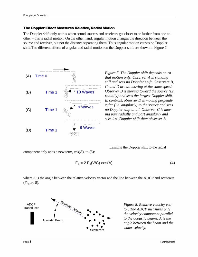
The Doppler Effect Measures Relative, Radial MotionThe Doppler shift only works when sound sources and receivers get closer to or further from one an-other – this is radial motion. On the other hand, angular motion changes the direction between thesource and receiver, but not the distance separating them. Thus angular motion causes no Dopplershift. The different effects of angular and radial motion on the Doppler shift are shown in Figure 7.

Limiting the Doppler shift to the radialcomponent only adds a new term, cos(A), to (3):

Fd = 2 Fs(V/C) cos(A) (4)

where A is the angle between the relative velocity vector and the line between the ADCP and scatterers(Figure 8).

Time 0

Time 1

Time 18 Waves

10 Waves

9 WavesTime 1

(A)

(B)

(C)

(D)

Figure 7. The Doppler shift depends on ra-dial motion only. Observer A is standingstill and sees no Doppler shift. Observers B,C, and D are all moving at the same speed.Observer B is moving toward the source (i.e.radially) and sees the largest Doppler shift.In contrast, observer D is moving perpendi-cular (i.e. angularly) to the source and seesno Doppler shift at all. Observer C is mov-ing part radially and part angularly andsees less Doppler shift than observer B.

Acoustic Beam

ADCPTransducer

Scatterer VelocityA

Scatterers

Figure 8. Relative velocity vec-tor. The ADCP measures onlythe velocity component parallelto the acoustic beams. A is theangle between the beam and thewater velocity.



3. BroadBand Doppler ProcessingSo far, we have looked at Doppler processing in terms of changes in frequency. BroadBand Dopplerprocessing, while equivalent mathematically, is easier to understand in terms of time dilation, that is, interms of changes to the signal in time rather than frequency. This section introduces the principles ofBroadBand signal processing.

Doppler Time DilationTo understand time dilation, consider sound scattering from a single particle. The echo from a pulse ofsound transmitted toward this particle will always look the same as long as the particle does not move.This result is illustrated in Figure 9A. If you move the particle a little further from the transmitter (Fig-ure 9B), you will see that it takes a little longer for the sound to go back and forth. If you move theparticle even more, it will take even longer (Figure 9C). This change in travel time caused by changingthe distance traveled is called the propagation delay.

Echoes from a single particle always look the same when the particle stays still — there is no propaga-tion delay. Echoes have the same relative phase which means zero phase change.

Two echoes superimposed: the second echo takes longer to return because the particle was furtheraway, hence it is delayed relative to the first echo. The delayed echo, shown with a dashed line, has aphase delay, relative to the first echo, of around 40º.

The second echo is delayed about 10 times as much as it was in example (B) because the particle movedabout 10 times as far. The longer propagation delay corresponds to a phase change of around 400º.

(A)

(B)

ScattererDisplacement

Echoes

Time Dilation

0º

40º

400º

PhaseChange

(C)

Figure 9. Propagation delay and phase change caused by scatterer displace-ment. Echoes are delayed when particles are farther from the sound source —this is called propagation delay. Propagation delay changes the relative phaseof the echo.



The principle of time dilation is simple: sound takes longer to travel back and forth when particles arefurther away from the transducer. A change in travel time, or a propagation delay, corresponds to achange in distance. If you measure the propagation delay, and if you know the speed of sound, you cantell how far the particle has moved. If you know the time lag between sound pulses, you can computethe particle’s velocity.

PhasePhase is a convenient and precise means to measure propagation delay. BroadBand ADCPs use phaseto determine time dilation. To understand phase consider the hands of a clock. One revolution of thehour hand corresponds to 360º of phase. One complete cycle (the time from one peak to the next) of asinusoidal signal corresponds to 360º of phase. Hence, the phase differences between the first and sec-ond echoes shown in Figure 9 are roughly (A) 0º, (B) 40º, and (C) 400º. These phase differences areexactly proportional to the particle displacements.

Time Dilation and Doppler Frequency ShiftFigure 10 shows that frequency shift and time dilation are equivalent. Figure 10A shows the echo fromtwo closely-spaced pulses returning from a stationary particle. If instead, the particle moves away fromthe transducer (Figure 10B), the time between the pulse echoes increases. This is because by the timethe second pulse arrives at the particle, the particle has moved further from the transducer; it thereforetakes longer for the sound to travel back and forth.

Figure 10. Time dilation and Dop-pler frequency shift. (A) and (B)compare echoes of pulse pairs fromstationary and moving particles. (C)and (D) show the same for the echofrom a sinusoidal pulse with a du-ration equal to the time between thetwo short pulses in (A) and (B). Thedashed lines indicate that thestretching is the same for the twopulses as it is for he sinusoid.

The same effect applies to a sinusoidal pulse (Figs. 10C and 10D). By the time the end of the sinusoidalpulse reaches the particle, the particle has moved further. This stretches the echo, changes the pitch ofthe echo, and thus causes a Doppler shift.

Many Doppler sonars measure frequency shift directly. BroadBand ADCPs use time dilation by meas-uring the change in arrival times from successive pulses. In reality, even though different measurementmethods involve different approaches, they are often mathematically equivalent. RDI engineers use

ScattererDisplacement

Echoes

(A)

(B)

(C)

(D)



phase to measure time dilation instead of measuring frequency changes because phase gives them amore precise Doppler measurement.

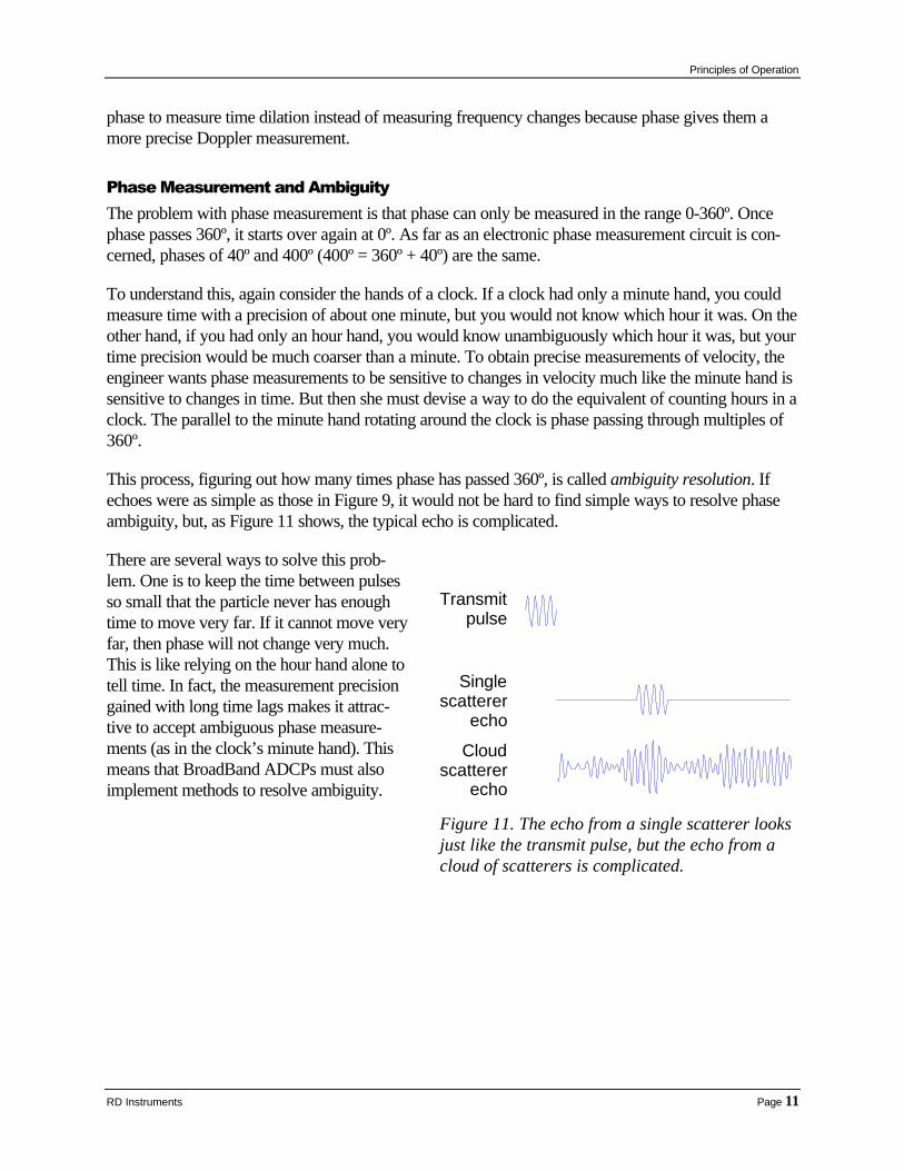
Phase Measurement and AmbiguityThe problem with phase measurement is that phase can only be measured in the range 0-360º. Oncephase passes 360º, it starts over again at 0º. As far as an electronic phase measurement circuit is con-cerned, phases of 40º and 400º (400º = 360º + 40º) are the same.

To understand this, again consider the hands of a clock. If a clock had only a minute hand, you couldmeasure time with a precision of about one minute, but you would not know which hour it was. On theother hand, if you had only an hour hand, you would know unambiguously which hour it was, but yourtime precision would be much coarser than a minute. To obtain precise measurements of velocity, theengineer wants phase measurements to be sensitive to changes in velocity much like the minute hand issensitive to changes in time. But then she must devise a way to do the equivalent of counting hours in aclock. The parallel to the minute hand rotating around the clock is phase passing through multiples of360º.

This process, figuring out how many times phase has passed 360º, is called ambiguity resolution. Ifechoes were as simple as those in Figure 9, it would not be hard to find simple ways to resolve phaseambiguity, but, as Figure 11 shows, the typical echo is complicated.

There are several ways to solve this prob-lem. One is to keep the time between pulsesso small that the particle never has enoughtime to move very far. If it cannot move veryfar, then phase will not change very much.This is like relying on the hour hand alone totell time. In fact, the measurement precisiongained with long time lags makes it attrac-tive to accept ambiguous phase measure-ments (as in the clock’s minute hand). Thismeans that BroadBand ADCPs must alsoimplement methods to resolve ambiguity.

Transmitpulse

Singlescatterer

echo

Cloudscatterer

echo

Figure 11. The echo from a single scatterer looksjust like the transmit pulse, but the echo from acloud of scatterers is complicated.



AutocorrelationAutocorrelation is a mathematical method useful for comparing echoes. While autocorrelation involvescomplicated mathematics, what it accomplishes is simple. Well-correlated echoes look the same anduncorrelated echoes look different. Autocorrelation is an efficient and effective method for detectingsmall phase changes.

RDI uses an autocorrelation method to process complicated real-world echoes to obtain velocity. Bytransmitting a series of coded pulses, all in sequence inside a single long pulse, we obtain many echoesfrom many scatterers, all combined into a single echo. We extract the propagation delay by computingthe autocorrelation at the time lag separating the coded pulses. The success of this computation re-quires that the different echoes from the coded pulses (all buried inside the same echo) be correlatedwith one another.

ModesADCPs implement a variety of modes with varying time lags and pulse forms. Default modes are cho-sen for robustness and measurement precision. Other modes are often able to produce even more ro-bust measurements (useful, for example, in highly turbulent water) or more precise measurements.Modes that produce highly precise measurements may work only in limited environmental conditions.They can also be more likely to fail when, for example, flow becomes rapid or turbulent.



4. Three-dimensional Current Velocity VectorsThe discussion so far has addressed single acoustic beams which can only measure a single velocitycomponent, the component parallel to the beam. This section explains how an ADCP uses four beamsto obtain velocity in three dimensions plus additional redundant (yet nevertheless useful) information.To use multiple beams to obtain velocity in three dimensions, one must assume that currents are uni-form (homogeneous) across layers of constant depth.

Multiple BeamsWhen an ADCP uses multiple beams pointed in different directions, it senses different velocitycomponents. For example, if the ADCP points one beam east and another north, it will measureeast and north current components. If the ADCP beams point in other directions, trigonometricrelations can convert current speed into north and east components. A key point is that one beamis required for each current component. Therefore, to measure three velocity components (e.g.east, north, and up), there must be at least three acoustic beams.

Current Homogeneity in a Horizontal LayerOne problem with using trigonometric relations to compute currents is that the beams make theirmeasurements in different places. If the current velocities are not the same in the different places,the trigonometric relations will not work. Currents must be horizontally homogeneous, that is,they must be the same in all four beams. Fortunately, in the ocean, rivers, and lakes, horizontalhomogeneity is normally a reasonable assumption.

Calculation of Velocity with the Four ADCP BeamsFigure 12 illustrates how we compute three velocity components using the four acoustic beams of anADCP. One pair of beams obtains one horizontal component and the vertical velocity component. Thesecond pair of beams produces a second, perpendicular horizontal component as well as a second ver-tical velocity component. Thus there are estimates of two horizontal velocity components and two es-timates of the vertical velocity. Figure12 shows the beams oriented east/westand north/south, but the orientation isarbitrary.

First pair of beamscalculates east-westand vertical velocity

Second pair of beamscalculates north-southand vertical velocity

East West North South

Beam velocity component

Currentvelocityvector

Figure 12. The relationship of beam and earth velocitycomponents.



Error Velocity: Why it is UsefulThe error velocity is the difference between the two estimates of vertical velocity. Error velocity de-pends on the data redundancy: only three beams are required to compute three dimensional velocity.The fourth ADCP beam is redundant, but not wasted. Error velocity allows you to evaluate whetherthe assumption of horizontal homogeneity is reasonable. It is an important, built-in means to evaluatedata quality.

Figure 13 shows two different situations. In the first situation, the current velocity at one depth is thesame in all four beams. In the second, the velocity in one beam is different. The error velocity in thesecond case will, on average, be larger than the error velocity in the first case. Note that it does notmatter whether the velocity is different because the ADCP beam is bad or because the actual currentsare different. Error velocity can detect errors due to inhomogeneities in the water, as well as errorscaused by malfunctioning equipment.

The Janus ConfigurationThe ADCP transducer configuration is called the Janus configuration, named after the Roman god wholooks both forward and backward. The Janus configuration is particularly good for rejecting errors inhorizontal velocity caused by tilting (pitch and roll) of the ADCP. This is because:

n The two opposing beams allow vertical velocity to cancel when computing horizontal velocity.

n Pitch and roll uncertainty causes single-beam velocity errors proportional to the sine of thepitch and roll error. Beams in a Janus configuration reduce these velocity errors to second or-der; that is, velocity errors are proportional to the square of the pitch and roll errors.

Non-Homogeneous Layer:Large error velocity

Current Vector

Homogeneous Layer: Zero error velocity

Figure 13. Non-homogeneous flow leads to large error velocity.



5. Velocity ProfileThe most important feature of ADCPs is their ability to measure current profiles. ADCPs divide thevelocity profile into uniform segments called depth cells (depth cells are often called bins). This sectionexplains how profiles are produced and some of the factors involved.

Depth CellsEach depth cell is comparable to a single current meter. Therefore an ADCP velocity profile is like astring of current meters uniformly spaced on a mooring (Figure 14). Thus, we can make the followingdefinitions by analogy:

n Depth cell size = distance between current meters

n Number of depth cells = number of current meters

There are two important differences between the string of current meters and an ADCP velocity pro-file. The first difference is that the depth cells in an ADCP profile are always uniformly spaced whilecurrent meters can be spaced at irregular intervals. The second is that the ADCP measures averagevelocity over the depth range of each depth cell while the current meter measures current only at onediscrete point in space.

Regular Spacing of Depth CellsRegular spacing of velocity data over the profile makes it easier to process and interpret the measureddata. This regular spacing is comparable to a regular sample rate. It is much more difficult to processirregularly-sampled data than it is to process data sampled uniformly in time. The same benefit appliesto measurements in a verticalprofile. Current Velocity Vector

Depthcell

Averages velocity withinentire depth cell

Measures Current Only at alocalized point

ADCP Moored Line ofstandard current meters

Figure 14. ADCP depth cells compared with conventional cur-rent meters.



Averaging Over the Range of EachDepth CellUnlike conventional current meters, ADCPsdo not measure currents in small, localizedvolumes of water. Instead, they average ve-locity over the depth range of entire depthcells. This averaging reduces the effects ofspatial aliasing. Aliasing in time series causeshigh frequency signals to look like low fre-quency signals. The effect is equivalent overdepth. Smoothing the observed velocity overthe range of the depth cell rejects velocitieswith vertical variations smaller than a depthcell, and thus reduces measurement uncer-tainty.

Range GatingProfiles are produced by range-gating theecho signal. Range gating breaks the re-ceived signal into successive segments forindependent processing. Echoes from farranges take longer to return to the ADCP than do echoes from closeranges. Thus, successive range gates correspond to echoes from in-creasingly distant depth cells.

The Relationship of Range Gates and Depth CellsA depth cell averages velocity over a range within the water column,but the averaging is usually not uniform over this range. Instead, thedepth cell is most sensitive to velocities at the center of the cell andleast sen sitive at the edges. The remainder of this section explainswhy this happens and describes the resulting weight function.

Figure 15 illustrates the relationship of range gates and depth cells.This plot relates time and distance from the ADCP. At the left side ofthe time axis is the transmit pulse. Transmit pulse propagation isshown with lines sloping up and to the right. Echo propagation backto the transducer is shown with lines sloping down and to the right.

As time increases, the transmit pulse propagates away from theADCP. Immediately after the transmit pulse is complete, the ADCPturns off the transducer and waits for a short time called the blankperiod. The ADCP now starts processing the echo corresponding toRange Gate 1. When Gate 1 is complete, the ADCP immediately be-

Ran

ge fr

om A

DC

P

Star

t

End

Transmitpulse

Gate 1 Gate 2 Gate 3 Gate 4

Echo Echo Echo Echo

Cell4

Cell3

Cell2

Cell1

Puls

e le

ngth

= ce

ll le

ngth

Time

Cell 1

Cell 2

Cell 3

Cell 4

Cell 5

0

Figure 15. Range-time plots hows how transmitpulses and echoes travel through space. Timestarts at the beginning of the transmit pulse andrange starts at the transducer face.

Sta

rt

End

Transmitpulse

Gate 1

Echo

Cell1

Cell2

Time

Cell2

Cell1

Echo

Gate 1

Transmitpulse

End

Sta

rt

A)

B)

Ran

ge fr

om A

DC

P

Figure 16. Range-time plot,detail.



gins processing Gate 2, and so on. These steps are shown on the horizontal axis.

To understand how Figure 15 works, first consider the echo of the leading edge of the transmit pulsefrom a scatterer located at the center of Cell 1. Follow the propagation line that marks the leading edgeof the transmit pulse — this line slopes up from the origin. Now find the line corresponding to theecho — this line slopes down from the intersection of the transmit pulse leading edge and the centerof Cell 1. These lines, shown in detail in Figure 16A, trace the passage of the leading edge of thetransmit pulse to the scatterer and the echo of this leading edge back to the transducer face. Figure 16Btraces the passage of the trailing edge of the transmit pulse to a different scatterer and its echo back tothe transducer. Both echoes arrive at the transducer at the beginning of Range Gate 1.

Once you understand the concepts presented in the previous paragraph, you can trace and study thepropagation paths that outline Cell 1. You can learn how the center of Cell 1 contributes the largestfraction of the echo signal to Range Gate 1. The echo from the farthest part of Cell 1 contributes signalonly from the leading edge of the transmit pulse. The echo from the closest part of Cell 1 contributessignal only from the trailing edge of the transmit pulse. You can also see how adjacent cells overlapeach other.

The Weight Function for a Depth CellScatterers in the center of the diamond-shaped space-time areas in Figure 15 contribute more energy tothe signal in Range Gate 1 than do scatterers near the top or bottom of the diamond. This means theyplay a larger role in determining the average current velocity measured in Gate 1. The velocity in eachdepth cell is a weighted average using the triangular weight functions in Figure 17. Note that eachdepth cell overlaps adjacent depth cells. This overlap causes a correlation between adjacent depth cellsof about 15%.

The above weight function applies to mostnormal situations for both narrowband andBroadBand ADCPs. However, when thetransmit pulse and depth cell sizes are differ-ent, the shape of the weight functionchanges. For example, if the transmit pulsewere short relative to the cell size, theweight function would be approximatelyrectangular with little overlap over adjacentcells. If the transmit pulse were longer thanthe depth cell, cells would overlap evenmore, and the data would be smoothedacross depth cells.

Center ofdepth cell

Increasing weight in depthcell averaging computation

Cell 3

Cell 2

Cell 1

Figure 17. Depth cell weight functions: depthcells are more sensitive to currents at the centerof the cell than at the edges.



6. ADCP DataThis section introduces and describes the data produced by a BroadBand ADCP. This data includes thefollowing four different kinds of standard profile data:

n Velocity

n Echo intensity

n Correlation

n Percent good

Velocity data are output in units of mm/s. Depending on your requirements, you can record data in oneof the following formats:

n Beam coordinates — Velocity is output parallel to each beam.

n Earth coordinates — Velocity is converted into north, east and up components.

n ADCP coordinates — Similar to earth coordinates except that velocity is converted to for-ward, sideways, and up components, relative to the ADCP. ADCP forward is the direction to-ward which beam 3 faces. ADCP sideways is to the right of forward. Figure 18 shows the typi-cal layout of a four-beam ADCP. Keep in mind that the view is looking at the face of theADCP. Beam 2 of a downward-looking convex ADCP points in the direction of a positivesideways velocity. Vertical velocities are positive upwards.

n Ship coordinates — Similar to ADCP coordinates except that heading is rotated into ship’sforward and sideways. If beam 3 faces toward the bow of the ship, ADCP and ship coordinatesare the same.

3

1

4

2

Forward

Figure 18. View facing an ADCPtransducer. The layout is the same forboth convex and concave transducers(see Figure 26).



Velocity transformations from beam coordinates to earth coordinates are described in more detail in thesection entitled ADCP movement: pitch, roll, heading, and velocity.

Echo intensity data are output in units proportional to decibels (dB). Data are obtained from the re-ceiver’s received signal strength indicator (RSSI) circuit.

Correlation is a measure of data quality, and its output is scaled in units such that the expected corre-lation (given high signal/noise ratio, S/N) is 128.

Percent-good data tell you what fraction of data passed a variety of criteria. Rejection criteria includelow correlation, large error velocity and fish detection (false target threshold). Default thresholds differfor each ADCP; each threshold has an associated command.

Bottom-track data are not profile data and they are output in a different part of the data structure, buttheir format is similar to the velocity profile data. The bottom-track coordinate transformation is identi-cal to the one used for the water profile. Bottom-track output also includes the vertical component ofthe distance, along each beam, to the bottom.



7. Ensemble AveragingSingle-ping velocity errors are too large to meet most measurement requirements. Therefore, data areaveraged to reduce the measurement uncertainty toacceptable levels. This section defines ADCP uncer-tainties, averaging methods, and the effect of aver-aging on data uncertainty.

ADCP Errors and Uncertainty DefinedVelocity uncertainty includes two kinds of error —random error and bias. Averaging reduces random er-ror but not bias.

Figure 19 shows these errors with two example dis-tributions of ADCP current estimates. Assume thatthe distribution in Figure 19A was computed from20,000 measurements of exactly the same current. Inthis distribution, the measurements cluster around theactual value of the current, but there is variation dueto the random error. Note also that the overall aver-age is different from the actual current. Bias causesthis difference.

Because random error is uncorrelated from ping toping, averaging reduces the standard deviation of thevelocity error by the square root of the number of pings, or:

Standard Deviation ∝ N-½ (5)

where N is the number of pings averaged together.

The distribution in Figure 19B shows what might happen if we were to make 200 ensembles of 100 pingseach from the original 20,000 pings. Averaging the 100 pings in each ensemble reduces the random error ofeach ensemble by a factor of about 1/10. This is clear in the smaller spread of the lower distribution. Notethat the average value of both distributions are the same and that both are different from the actual current.This difference, that does not go away with averaging, is the measurement bias.

An important point is that averaging can reduce the relatively large random error present in single-pingdata, but that, after a certain amount of averaging, the random error becomes smaller than the bias. Atthis point, further averaging will do little to reduce the overall error.

Mean Value of ADCP Estimates

ADCP Bias

Actual Current

Distribution of Ensemble-AveragedADCP Current Estimates

Distribution of Single-PingADCP Current Estimates

Actual Current

ADCP Bias

Mean Value of ADCP Estimates

(A)

(B)

Figure 19. The distribution of single-pingdata (A) compared with the distribution of200-ping averages of the same data (B).



Short- Vs. Long-Term UncertaintyShort-term uncertainty is defined as the error in single-ping ADCP data. Short-term uncertainty isdominated by random error.

Long-term uncertainty is defined as the error present after enough averaging has been done to essen-tially eliminate random error. Long-term error is the same as bias.

The Approximate Size of Random Error and BiasADCP single-ping random error or short-term error can range from a few mm/s to as much as 0.5 m/s.The size of this error depends on internal factors such as ADCP frequency, depth cell size, number ofpings averaged together and beam geometry. External factors include turbulence, internal waves andADCP motion.

Random error in narrowband ADCPs is relatively easy to estimate, but it is harder to estimate forBroadBand ADCPs. This is because BroadBand measurements have more adjustable parameters, eachof which affects uncertainty. Because random errors generated internally in the ADCP are typically anorder of magnitude smaller than in a comparable narrowband ADCP, external random error sources(i.e. turbulence) can dominate internal ADCP errors.

You can estimate random errors by computing the standard deviation of the error velocity. This is be-cause random errors are independent from beam to beam and because the error velocity is scaled by theADCP to give the correct magnitude of horizontal-velocity random errors. To predict the size of inter-nal random errors, consult brochure specifications or use one of the various software tools that RDIprovides for this purpose.

Bias is typically less than 10 mm/s. This bias depends on several factors including temperature, meancurrent speed, signal/noise ratio, beam geometry, etc. It is not yet possible to measure ADCP bias andto calibrate or remove it in post-processing.

Beam Pointing ErrorsBeam pointing errors can be a dominant source of velocity bias. A beam pointing error is uncertainty inthe beam direction. Standard manufacturing practice introduces errors into beam angles. Depending onmeasurement requirements and the care with which the transducer elements were installed, these errorscould introduce unacceptable bias. The as-installed beam angles are measured in the manufacturingprocess and stored in the BroadBand ADCP’s memory. These angles modify the coordinate conver-sion matrix which corrects for beam pointing errors when converting from beam to earth velocity co-ordinates.

Averaging Inside the ADCP Vs. Averaging LaterAn ADCP system can calculate ensemble averages inside the ADCP, in the data acquisition system, orin both. It is possible, for example, to average ensembles of several pings in the ADCP and to send theresults to a computer which then computes averages of these ensembles. Normally, unless there is agood reason to do otherwise, the best rule is to let the ADCP convert data into earth coordinates and



to average data into ensembles before transmitting them out. Following is a list of the factors that mightaffect your choice of where to average your data.

n Vector averaging — Conversion to earth coordinates prior to averaging allows the ADCP tocompute true vector averages.

n Beam pointing errors are automatically corrected when the ADCP converts from beam to earthcoordinates, thus minimizing related biases.

n Data transmission takes time and can slow down ping processing. Averaging reduces the timerequired for data transmission.

The Processing Cycle: Limitations on AveragingAveraging is limited by the ping rate, which is limited by how fast the ADCP can collect, process andtransmit data. Figure 20 shows a typical data collection cycle inside the ADCP. Each ping has fivephases: overhead, transmit pulse, blank period, processing, and sleep. The overhead time is used towake up the ADCP, initialize and process various subsystems (e.g. the clock, compass, etc.) and toprepare for ping processing. After pulse transmission and a short delay to allow the transducer to ringdown (see later), the ADCP begins to process the echo. When echo processing is complete, the ADCPeither goes to sleep to conserve battery power or immediately begins another data collection cycle.After all the pings are collected, the ADCP computes an ensemble average and transmits the data tothe internal data recorder, to an external data acquisition system, or to both. When the ADCP pingsrapidly, data transmission runs in the background, using CPU time when it is free.

* Processing time depends on: 1. What processing is done 2. Number of cells 3. Speed of sound 4. Computation time

Ove

rhea

dTr

ansm

it pu

lse

Proc

essi

ng *

Slee

p

Single ping

First ping Second pingData

transmission

Ensemble of pings

Blan

k

Figure 20. Steps in the ping processing cycle



8. ADCP Pitch, Roll, Heading and VelocityADCPs measure currents relative to the ADCP. The ADCP itself can be oriented arbitrarily and mov-ing relative to the earth. Therefore, it is usually necessary to correct the data for ADCP attitude andmotion. This section covers why ADCP data require correction and how to measure and correct forADCP motion and attitude.

There are two kinds of motion that require correction — rotation (pitch, roll, and heading) and transla-tion (ship velocity).

Conversion from ADCP- to Earth- Referenced CurrentThe following are three general steps in the conversion from ADCP- referenced currents to earth- ref-erenced currents

Step 1. ADCPs measure velocity parallel to the four acoustic beams (beam coordinates). These data areconverted into an orthogonal coordinate system of ADCP north, east, and up. This correction adjustsfor the angle of the beams (trigonometry) as well as the fact that depth cells of a tilted ADCP (Figure21) move up and down relative to one another. Correction includes the following:

n Trigonometry. The beam angle used or correction (see Eq. 4) is the sum of the ADCP beammounting angle (i.e. 20º) plus (or minus) the tilt angle.

n Depth cell mapping. To ensure horizontal homogeneity, the calculated velocity at a particulardepth uses cells that are at the same depth. Figure 21B shows the depth cells of a tilted ADCP.Note, for example, that depth cell 4 on the left beam is at the same depth as depth cell 6 on theright beam. Depth cell mapping matches these two cells together to compute earth velocity atthis depth. (Note: depth cell mapping was implemented for BroadBand firmware versions 5.0and later.)

Step 2. The ADCP rotates velocity components into true (or magnetic) east and north (earth coordi-nates). This correction requires headingdata.

Step 3. ADCP velocity relative to theearth is subtracted, providing absolute,earth-referenced currents. This correctionrequires measurements of the ship’s ve-locity relative to the earth. Subtraction isnormally done after the data are collectedand recorded.

In practice, these steps are not alwaysdone in the above order, and they are notnecessarily separated into discrete steps. Pitch or roll angle

Depth cells

Depth cellmapping

Cellschangedepth

(B)(A)

Figure 21. ADCP tilt and depth cell mapping



Measuring ADCP Rotation and TranslationThere are many ways to measure rotation and translation. The following are commonly used withADCPs:

Rotation (heading)1. Flux-gate compass2. Gyrocompass

Rotation (pitch and roll)1. Inclinometers2. Vertical gyro

Translation1. Bottom-tracking2. Navigation device (i.e. GPS)3. Assume a “layer of no motion” (reference layer)

Self-Contained and Direct-Reading ADCPsSelf-Contained and Direct-Reading ADCPs are designed for use where motion is relatively slow andunaffected by surface waves. In such an environment a flux-gate compass and inclinometers can effec-tively measure pitch, roll, and heading. These sensors are used because of their small size (they fit in-side the ADCP pressure case) and low power consumption (necessary for Self-Contained ADCPs).These sensors have the following limitations:

Flux-gate compasses cannot be used near ferrous materials, such as a ship’s steel hull, that would affectthe earth’s magnetic field. Some flux-gate compasses are noisy when affected by accelerations of sur-face waves.

Inclinometers measure tilt relative to earth gravity, but cannot differentiate the acceleration of gravityfrom accelerations caused, for example, by surface waves. Hence, inclinometers can be noisy in movingboats.

Both BroadBand and Workhorse compasses are sensitive to motions, either directly (as in theBroadBand compass) or indirectly through their inclinometers.

Data Correction Strategies for Self-Contained ADCPsSelf-Contained ADCPs can be mounted on moorings where they are free to change orientation, or inframes on the sea bottom where their orientation is fixed. These two methods call for different datacorrection strategies.

Moored ADCPs should convert each ping into earth coordinates prior to averaging. This ensures thatensemble averages are vector averages. Earth-coordinate averaging is equivalent to vector-averaging instandard single-point current meters, and it ensures that the data have both the best accuracy and high-est resolution possible given the depth cell size.



When an ADCP is mounted on the sea bottom, you could choose to record data either in beam coordi-nates or in earth coordinates. Recording data in earth coordinates reduces the time and effort requiredfor post-processing and it ensures that beam pointing angles are properly corrected. Recording data inbeam coordinates allows you to record the least-processed data, and it allows them to optimize theprocessing used to convert the data to earth coordinates. However, proper correction for beam point-ing angle errors can be time-consuming to implement and debug.

Correction for beam pointing angle errors is more important for the Workhorse than for theBroadBand because the Workhorse manufacturing process allows wider tolerances for transducer in-stallation. Without correction, errors can be significant.

Vessel-mounted ADCPsThe remainder of this section applies to vessel-mounted ADCPs in which the transducer is permanentlyinstalled on the hull. It applies equally to direct-reading ADCPs that are temporarily mounted on thehull. Procedures used once at the time of installation of a standard vessel-mounted ADCP must be fol-lowed each time a direct-reading ADCP is reinstalled on a ship.

Gyrocompasses and vertical gyros are used on ships because they are unaffected by horizontal accel-erations from surface waves. Inclinometers are sometimes used in ships, but it is not good practice touse the raw inclinometer data to correct each ping. Instead, the average pitch and roll may be used todetect variation in mean tilts caused by changes in ballasting, propeller speed, etc.

There are many different ways for ADCPs to obtain attitude information from gyros, but this flexibilityis limited by the need to obtain tilt and heading at exact times during ping processing. Most often,ADCPs use a synchro interface to measure pitch, roll and heading angles. ADCPs also obtain headinginformation through a stepper interface.

Direct-reading ADCP deck boxes with synchro interfaces send their data to the ADCP via a serial in-terface using a proprietary format. RDI does not yet support sending attitude data into an ADCP usingindustry-standard formats, but some software programs (i.e. TRANSECT) can accept serial attitudedata in NMEA formats. Keep in mind that, while ships often digitize attitude on a regular time interval(e.g. every second or ten seconds), the ADCP has no control over data sampling and therefore cannotsynchronize the attitude data with the pings.



SynchrosA synchro interface enables ADCPs to get heading data at the exact time it is required. Synchros aremotors that are normally used in pairs. When one synchro rotates a given amount, the other rotates thesame amount. The synchro interface uses five wires for the following synchro outputs:

n Three “sense” outputs — S1, S2, and S3

n Two “reference” outputs — R1 and R2

The outputs have AC voltages that vary depending on the synchro rotation angle. The synchro voltage isexpressed as the maximum voltage between any pair of sense outputs. Synchros are commonly powered by110 VAC, in which case the maximum voltage between sense outputs will be 90 VAC. This is a 90-volt syn-chro. Standard synchro voltages include:

n 90 VAC

n 26 VAC

n 11.8 VAC

Other voltages are rarely used, but the ADCP synchro interface can work with any voltage between 11.8 and90 VAC. Adjustment is made by changing the value of a precision resistor network in the interface. The fre-quency of a synchro can have an average value between 50 and 1000 Hz.

Multiple Turn Synchros for HeadingIt is common for gyrocompasses to use multiple-turn synchros for output. For example, a multiple-turnsynchro with a 360:1 turns ratio would rotate 360 times every time the ship rotates once. Commonturns ratios are:

n 360:1

n 90:1

n 36:1

n 1:1

RDI’s synchro interface uses any of the above. If the turns ratio is other than 1:1, the ADCP must ini-tialize the synchro interface to the correct starting direction. For example, with a 36:1 synchro, the syn-chro makes one complete revolution each time the ship turns 10º. The ADCP cannot tell the differencebetween 313, 13, 23, etc. This means the operator must set the ADCP system for the correct anglewhen the ADCP starts up. This is most easily handled via a panel interface on either the direct-readingor vessel-mounted ADCP deck boxes.

It is normally best to use a 1:1 synchro interface whenever possible for the following reasons:n The accuracy of a 1:1 synchro is normally sufficient.

n If power is lost, synchro turns ratios other than 1:1 require reinitialization.

Pitch and roll synchros must use 1:1 turns ratios.



Correction for Ship VelocityWhen available, absolute ship velocity is recorded along with the water velocity profiles. Later, duringpost-processing, the ship velocity can be subtracted from the current profile data. There are three waysto measure ship velocity:

1. Bottom-tracking2. Navigation3. Assuming a “layer of no motion” (reference layer )

Bottom-tracking can only be used when the bottom is within the ADCP’s bottom-tracking range —this is about 1.5 times the normal profiling range. When bottom-tracking is unavailable, navigation canbe used to estimate ship velocity. Trade-offs of the various kinds of navigation systems are discussedbelow.

Using a reference layer involves assuming that a layer within the profiling range of an ADCP has nomotion. The utility of this assumption depends upon the site where the measurements are made.

Effects of Correction on Vessel-Mounted ADCP MeasurementsThis section covers the following two kinds of motion that limit a vessel-mounted ADCP’s data quality:

n Pitch and roll motions of the ship in surface waves

n The large ship speed compared with the measured currents.

It turns out that pitch and roll are of less concern than one might think. Kosro (1985) used an ADCP tomeasure currents and a gyro to measure pitch and roll on a ship offshore northern California. He re-corded raw ADCP pings along with simultaneous gyro data, and then computed current profiles bothwith and without pitch and roll correction. He found the following results:

n Corrected and uncorrected horizontal currents were different with a bias of about 1 cm/s. Theuncorrected data were also smoothed over a depth range about equal to the distance that depthcells moved up or down as a result of the pitch and roll.

n Corrected and uncorrected vertical currents were different by as much as 5 cm/s.

Therefore, we conclude that pitch and roll correction is required only in the following circumstances:

n When the greatest possible data accuracy is required.

n When the ship is expected to encounter severe wave conditions.

n When accurate vertical velocity components are required.



Correction of ADCP data for the speed of the ship can vary from relatively easy to quite difficult. Theeasiest correction is when bottom-track data are available. Correction with bottom-tracked ship veloc-ity is relatively easy to do well because:

n Bottom-track velocity data are usually more accurate than the current profile data.

n The bottom-track velocity and current profile velocity are measured in the same coordinatesystem.

Bottom-tracking’s biggest advantage is that many of its largest errors are matched by exactly the sameerrors in the current profile. These common-mode errors then cancel exactly when bottom-track veloc-ity is subtracted from the current profile data. Major common-mode errors include compass errors andvelocity biases caused by beam pointing errors. This advantage arises from the fact that bottom-tracking and current profiling use the same coordinate system

In contrast, ship’s navigation and current profiling share no common-mode errors. For example, errorsof 1º or more are common in ship’s gyros. A 1º compass error introduces a sideways velocity error ofalmost 10 cm/s when a ship steams at 5 m/s.

Heading errors are caused by the following:

n Transducer misalignment. This is a result of the difficulty in measuring the orientation of thetransducer in the ship. In fact, the transducer need not be oriented in any specific direction, butthe orientation must be known. For more information on in-situ transducer orientation calibra-tion, refer to Pollard and Read (1989) or Joyce (1988).

n Gyro errors and instability. This depends on the make and model of the gyrocompass. Onesource of error is the Schuler oscillation, a direction error with a period of 84 minutes and anamplitude of typically 0.5º—1.0º. The Schuler oscillation is often excited when the ship makesa turn.

The accuracy of navigation correction depends strongly on the navigation used. Differential GPS isgenerally the best choice for overall accuracy and easy use. However, bottom-tracking usually pro-duces smaller short-term errors than even the best GPS.



9. Echo Intensity and Profiling RangeEcho intensity is a measure of the signal strength of the echo returning from the ADCP’s transmit pulse.Echo intensity is sometimes used to survey the concentration of zooplankton or suspended sediment. RDIhas not yet developed procedures for absolutely calibrating BroadBand backscatter measurements, butBroadBand ADCPs (including Workhorses) are useful for relative measurements. This section introducessome of the factors involved in interpreting and using backscatter data.

Echo intensity depends on:

n Sound absorption

n Beam spreading

n Transmitted power

n Backscatter coefficient

An approximate equation for echo intensity is:

EI = SL + SV + constant - 20log(R) -2αR (6)

where:

EI is the echo intensity (dB)SL is the source level or transmitted power (dB)SV is the water-mass volume backscattering strength (dB)α is the absorption coefficient (dB/meter)R is the distance from the transducer to the depth cell (meters)

The constant is included because the measurement is relative rather than absolute. This means theADCP sees variations in echo intensity, but it cannot make absolute measurements that can be com-pared with other ADCPs. The term 2eR accounts for absorption and 20log(R) accounts for beamspreading.

Keep in mind that the relationship of echo intensity to particle concentration strongly depends on theparticle size. This means that you must calibrate the relationship between echo intensity and concentra-tion with in-situ measurements. When the particle size distribution is variable, it may not be possible tosatisfactorily calibrate this relationship.

The maximum range of the ADCP corresponds to the location where the signal strength drops to levelscomparable to the noise level. Beyond this range the ADCP cannot accurately calculate Doppler shifts.The remainder of this section will review factors that affect both the signal strength as a function ofrange from the ADCP and the overall range of the ADCP.



Sound AbsorptionAbsorption reduces the strength of echoes as a result of physical and chemical processes in water. Ab-sorption in the ocean is more rapid than in fresh water, primarily because of chemical reactions. Ab-sorption causes a linear reduction (proportional to 2eR above) of echo intensity with range whenmeasured in dB. This means that absorption causes echo intensity to decay exponentially with increas-ing range.

Sound absorption (in dB/meter) increases roughly in proportion to frequency within the frequencyrange in which ADCPs operate (75-1200 kHz; see Table 1 or Urick, 1983). This produces an inverserelationship between frequency and range.

Frequency (kHz) α(dB/m) Nominal Range (m) @ Power (W)

76.8 0.022-0.028 700 250

153.6 0.039-0.050 400 250

307.2 0.062-0.084 120 80

614.4 0.14-0.20 60 30

1228.8 0.44-0.66 25 15

The sound absorption values given in Table 1 come from Urick (1983) and Kinsler, et al. (1980). Therange shown more likely represents uncertainty in the true absorption rather than the actual variationpresent in the ocean.

Table 1. Sound absorption (At 4ºC, 35‰ and at sea level) and nominal pro-filing range of a BroadBand ADCP. The transmit power listed is the maxi-mum power that can be transmitted subject to limitations caused by shockformation.



Beam SpreadingBeam spreading is a geometric cause for echo attenuation as a function of range. In Equation 6 above,beam spreading is represented as a logarithmic loss in echo intensity with increasing range, where echointensity is measured in dB. In linear units, the echo intensity decreases proportional to the rangesquared.

An explanation for this range-squared behavior is shown in Figure 22. Doubling the distance to a scat-terer causes the scatterer to intersect one-quarter as much of the total sound energy in the beam. Thus,it reflects back one-quarter as much energy. However, because the beam has four times the area, therewill be four times as many scatterers reflecting sound back, keeping the total reflected energy constant.The reduction in echo intensity is the result of the transducer intersecting only one-quarter as much ofthe total reflected energy as before.

Source Level and PowerThe source level of a BroadBand signal depends on the following factors:

n Power. The ADCP’s transmit power is normally proportional to the square of the transmitvoltage. The primary difference between low and high-power ADCPs is the voltage applied tothe transducer. If the voltage is regulated (i.e. in high-power BroadBands), the transmit powergoing into the transducer stays constant. The transmit power of a Workhorse ADCP, however,is taken directly from its DC input. Thus, its transmit power is proportional to the square of theinput voltage. Transmit power also depends on stored energy. High-power BroadBand ADCPsuse large banks of capacitors to supply power for long bottom-track pulses. If the ADCP hasinsufficient capacitance, the power falls while the pulse is being transmitted.

n Transducer efficiency. The transducer controls transmit power through its efficiency. Typicalefficiencies range from 25-80%.

Reflected acoustic beam

Transducer Transducer

Scattering layer

Scattering layer

Figure 22. Range-dependent signal attenuation



n Transmit pulse. Longer transmit pulses put more energy into the water. In addition, pulsecoding can reduce the average power transmitted. Codes normally just switch phase (by multi-plying by ±1) but otherwise sustain constant power. However, the average power can be re-duced by using codes that include zeros instead of only ±1.

n Shock. As sound intensity increases, it reaches a point where it becomes nonlinear. Non-linearacoustics (shock formation) rapidly attenuates sound, effectively reducing energy to levels nearthe maximum possible without shock formation. Shock formation tends to limit transmit en-ergy primarily at 300 kHz and above.

n Cavitation. At lower frequencies (150 kHz and below), large amplitude acoustic pressurefluctuations cause pressures so low that vapor bubbles form momentarily. These bubbles col-lapse noisily, seriously degrading ADCP performance. Cavitation is a problem primarily onfast-moving ships.

ScatterersThe concentration of scatterers affects range because more scatterers reflect more sound. The domi-nant oceanic sound scatterer at ADCP frequencies is zooplankton with sizes on the order of one milli-meter (Figure 4 shows some typical zooplankton). Other scatterers can include suspended sediment,detritus, and density gradients (though density gradients are relatively weak scatterers).

On occasion, the lack of scatterers in the water reduces the range relative to the nominal range. In oneextreme example, the range was about one-third of the nominal range (on a cruise by the Institute ofOcean Sciences, Wormley, UK, using an RD-VM0150 near Mauritius). Such instances have been un-common, occurring less than 10% of the time.

ADCPs used at depths below 1200 m often experience range reductions to as little as one-third normalrange.

BubblesIn rough seas, breaking waves generate bubbles below the ocean surface. When bubbles pass under theship’s hull, they can act as a shield, inhibiting the transmission of sound. Bubbles sometimes reduceprofiling range, and in extreme cases, bubbles block the signal completely.



10. Sound Speed CorrectionsAn ADCP computes sound speed based on an assumed salinity and transducer depth and on the tem-perature measured at the transducer. The ADCP uses this sound velocity to convert velocity data intoengineering units and to compute distances along the beams. The sound speed is recorded along withthe other ADCP data. This section describes corrections you may make for sound speed variations anderrors.

Correction for Variation in Speed of Sound at the TransducerVelocity data are output in units of mm/s. The velocity scale factor is proportional to the speed ofsound measured at the transducer. The ADCP automatically computes sound speed given the meas-ured temperature and an assumed salinity. If it is in error (i.e. if the assumed salinity is wrong), velocitycan be corrected for sound speed in post processing by using the following equation:

Vcorrected = Vuncorrected (Creal/CADCP) (7)

where Creal is the true sound speed at the transducer and CADCP is the sound speed recorded by theADCP.

You may use the following equation to compute sound speed (Urick, 1983):

C = 1449.2 + 4.6T -0.055T2 + 0.00029T3 + (1.34 - 0.01T)(S - 35) + 0.016D (8)

where:

T is the temperature in ºCS is salinity in parts per thousand (‰)D is the depth in meters

Variations in sound speed with depth (e.g. away from the transducer) do not affect calibration, as willbe shown later.



Correcting Depth Cell Depth for Sound Speed VariationsThe ADCP computes depth cell locations by assuming that the sound speed is constant over the watercolumn. In so doing, the ADCP automatically accounts for the transducer beam angle (20º or 30º).

When range is large and sound speed differs from the speed at the transducer, the depth of each depthcell may be corrected if the sound speed profile is known. One procedure for doing this consists of thefollowing steps:

n Determine the position of the first depth cell

n Determine the length of the depth cell using the equation:

L corrected = L uncorrected (CADCP /Creal ) (9)

where L is the depth cell length.

n Using the above depth cell length, determine the position of the next depth cell.

n Repeat this process for all depth cells.



11. TransducersTransducer quality is essential for data quality. ADCPs place unusually high demands on transducers.They must be directional (including both narrow beamwidth and suppressed side lobes) and efficient.BroadBand processing requires 25-50% bandwidth, and deep deployments require that the transducerwithstand extreme pressures. This section describes transducer characteristics, particularly those thataffect measurement performance.

The active elements in transducers are piezoelectric ceramic disks that expand or contract under theinfluence of an electric field. The electric field is applied through thin layers of silver deposited on thesurfaces of the ceramic. When a voltage is applied, the disk gets thicker or thinner, depending on thepolarity of the voltage.

The ceramic disk is potted (encased) with polyurethane in a metal cup with a reflective backing mate-rial. Self-Contained ADCPs are designed for high pressure, using an incompressible backing material sothat the transducer will not break under pressure.

Transducer Beam PatternThe transducer beam pattern shows the strength of transmitted sounds far from the transducer as afunction of the angle. The angle is measured relative to the transducer axis, a line drawn from the cen-ter of the transducer perpendicular to the transducer face. The beam pattern is reciprocal in that it rep-resents equally well the transducer’s sensitivity to incoming sound as a function of direction.

Figure 23 shows an example transducer beampattern. The main lobe points in the directionof the transducer axis, defined to be 0º. Mostof the energy passes through the main lobe.The beamwidth is the width of the main lobe atthe -3 dB level (-3 dB corresponds to half thesignal strength).

Side lobes point in directions different from themain lobe. Outside of 15º from the main lobe,side lobes are suppressed by typically 35 dB ormore relative to the main lobe. The size of theside lobes depends on the size of the trans-ducer as well as the details of its manufacture.If the transducer is larger (at a given fre-quency), the beam becomes narrower, and sidelobes are suppressed.

Some side lobes do not depend on transducer size, but result instead from modes of vibration in thepiezoelectric ceramic. It is common to find side lobes at about 40º from the main lobes, and these sidelobes can be dominant error sources.

0

-20

-40

-60

-90 -60 -30 0 30 60 90Direction (degrees)

Tra

nsdu

cer

resp

onse

(dB

)

Figure 23. Typical beam pattern of a 150 kHztransducer. Transducer response is one-way,measured relative to the response at the trans-ducer axis.



The transducer beam pattern shown in Figure 23 is a one-way beam pattern because it shows thestrength of the transmitted sound. The sensitivity of the transducer to echoes is characterized bytwo-way transducer beam patterns because the transducer both transmits and receives sound. Thetwo-way beam pattern is simply double (in dB) the one-way beam pattern. Therefore side lobes thatare suppressed by 40 dB in the one-way pattern are suppressed by 80 dB in the two-way pattern. En-ergy reflected from these directions is suppressed by a factor of 100,000,000 relative to the main lobe.

Table 2 lists dimensions and characteristics of some of RDI’s transducers.

Table 2. Characteristics of some typical Broadband ADCP transducers

Frequency(kHz)

Wavelength(mm)

Transducer diam.(mm)

Beamwidth at-3dB

Avg. Side lobelevel

76.8 20 280 5.0° .36 dB

153.6 10 165 4.0° .36 dB

307.2 5 133 2.2° .41 dB

614.4 2.5 101 1.5° .42 dB

1228.8 1.25 54 1.4° .42 dB



Transducer ClearanceObstructions in front of transducers can interfere with the acoustic beams and degrade data quality.Figure 24 shows the region in which you must eliminate all obstructions.

TRANSDUCER CUP

15°

Figure 24. Keep obstructions out of the shaded re-gion in front of the transducer. This region in-cludes a 15º cone around the transducer.



Measurement Near the Surface or BottomThe echo from a hard surface such as the sea surface or bottom is so much stronger than the echo fromscatterers in the water that it can overwhelm the side lobe suppression of the transducer. You shouldnormally reject data from distances too close to the surface (when looking up) or bottom (when look-ing down). Figure 25 shows transducer beam angles oriented 20º and 30º from vertical. For the 20ºtransducer, the echo through the side lobe facing the surface returns to the ADCP at the same time asthe echo from the main lobe at 94% of the distance to the surface. This means data from the last 6% ofthe range to the surface can be contaminated. The concept is the same for a 30º transducer except thatcontamination covers a greater fraction of the range (15%). The effect is the same for an ADCP at thesurface looking down to the bottom.

The equation that governs this is:

Rmax = D cos(θ) (10)

where:

Rmax is the maximum range for acceptable dataD is the distance from the ADCP to the surface or bottom (as appropriate)Angle θ is the angle of the beam relative to vertical (normally 20º or 30º)

85%

15% contaminated

30º

94%

6%

Mai

n lo

be

Sid

e lo

be

20º

Figure 25. The relationship between transducer beam angle and thethickness of the contaminated layer at the surface.



When looking down, contamination from bottom echoes usually biases velocity data toward zero. In amoving vessel, contamination from bottom echoes is less predictable. When looking up, contaminationfrom surface echoes is unpredictable as a result of surface waves and winds, but a bias toward zero iscommon. The velocity of the surface or the bottom is zero on average; it is this zero velocity that biasesthe measured velocity toward zero.

RingingRinging is an effect in which energy from the transmit pulse lingers after the transmit pulse is finished.If there were no ringing, the transducer could receive echoes immediately after transmitting. However,echo signals are weak and it does not take much ringing to contaminate the echoes. Thus, the ADCPmust wait for the ringing to die away before it can listen to and process the echoes. This waiting time iscalled the blanking period. Table 3 shows typical ringing times. These ringing times are approximatelyequal to the default blanking period.

Frequency Ringing distance

75 kHz 6 m

150 kHz 4 m

300 kHz 2 m

600 kHz 1 m

1200 kHz 0.5 m

Ringing biases velocity data toward zero velocity because the ringing signal is not Doppler-shifted.Sources of ringing include:

n Receiver electronicsn Transducer and/or electronics housingn Sea chest in a shipn Ship’s hull

In general, plastic housings ring less than metal housings. Sea chests covered with acoustic windowsreflect sound around inside and thus cause greater ringing. Ringing is a problem in low backscatter be-cause the ringing energy stays above the weak echo signals longer.

Table 3. Typical ringing times, expressed as distances infront of the transducer.



Ringing tends to be a more serious problem on ships than in other applications. You can minimizeringing in ships by taking the following steps:

n Mount the transducer on a material with a large acoustic impedance mismatch between themetal transducer and the metal hull. This reduces the sound energy that gets into the hull.(Note: be careful when choosing material for acoustic impedance. Some common materials,such as syntactic foam, that would appear to mismatch water’s acoustic impedance are, in fact,surprisingly close!).

n Line sea chests with acoustically-absorbent material to attenuate sound bouncing around insidethe sea chest.

n When acoustic windows are used, choose window materials that match the water’s acousticimpedance to help minimize reflections within the sea chest.

RDI provides a test program to measure ringing in vessel-mounted ADCPs.

PressureRDI direct-reading and self-contained transducers are designed to withstand full-ocean-depth pres-sures. Our limited experience at depths greater than 2000 meters suggests that the transducer’s per-formance is relatively unaffected, but that low backscatter tends to reduce range.

Concave vs. ConvexSelf-Contained and Direct-Reading ADCPs use convex transducers (Figure 26) to allow the ADCP tobe mounted in an in-line mooring cage. Vessel-Mounted ADCP transducers are concave to allow themto be mounted inside the smallest possible sea chest in the ship’s hull.

Sea Chest

Vessel-Mounted ADCPConcave Transducer

Self-Contained or Direct-Reading ADCPConvex Transducer

Mooring Line

Figure 26. Concave and convex transducers.



12. Sound Speed and ThermoclinesThis section addresses the effects of depth variations in sound speed and of thermoclines on data qual-ity. Neither significantly impair data quality.

Sound Speed Variation with DepthVariation of sound speed with depth does not affect measurement of horizontal currents. In simpleterms, sound speed variation has two effects that exactly counteract one another. The effect of chang-ing sound speed is to refract or bend the sound beams, but the bend is exactly the right amount to pre-serve the accuracy of the horizontal current (Figure 27).

The theoretical basis for this result is Snell’s law, which says that horizontal wavenumber is conservedwhen sound passes through horizontal interfaces. Figure 27 shows that sound waves are continuousacross the horizontal interface. Because the frequency remains constant, sound speed variation doesnot affect the horizontal component of sound velocity. And because measurement of the horizontalcurrent depends directly on the horizontal sound speed, the horizontal current measurement is unaf-fected.

In contrast, variations in the vertical velocity component are proportional to variations in sound speed.

Sound wave direction

Horizontal component (remains constant)

Wavelength

Wav

eleng

th

Dep

th

Speed of sound = wavelength x frequency (increase) (increase) (no change)

Figure 27. How sound speed variations with depth affects sound propagation. Eventhough the sound wave direction changes with depth (via refraction), the horizontal soundvelocity remains constant.



ThermoclinesWhile strong thermoclines sometimes block sonar penetration, ADCPs can always penetrate the ther-mocline. The reason ADCPs can always penetrate the thermocline is that their beams are relativelysteep, pointing more vertical than horizontal. Sonars that have trouble penetrating the thermocline havebeams that are closer to horizontal. Such difficulties arise, for example, when a ship is trying to find asubmarine near the thermocline (Figure 28).

30 º

60 º

Thermocline layer

ADCP beams

Figure 28. The effect of strong thermoclines on sound propagation.



13. Bottom TrackingMost of this primer addresses water velocity profiling. This section describes how bottom-trackingcompares to velocity profile measurements and how bottom-tracking is implemented.

Difference Between Bottom-Tracking and Water-ProfilingWhile water-profiling uses short transmit pulses to obtain vertical resolution, bottom-tracking requireslong pulses. Long pulses are used to allow the sound beam to ensonify the bottom over the entire beamall at once (Figure 29). If the pulse is too short, the echo returns first from the leading edge of thebeam, followed later by the trailing edge. Because the beam has a finite beamwidth, the angle of thebeam relative to horizontal is different on these two edges. This means that the Doppler shift is differ-ent from one side of the beam to the other. By illuminating the bottom across the beam all at once, along pulse produces an accurate and stable estimate of velocity, more accurate than is typically ob-tained from water profiles.

The downside of long transmit pulses is that a considerable part of the echo can come from water-mass ech-oes. Where water-mass echoes are weak relative to the bottom echo, this causes no problem, but in placeswith high concentrations of suspended sediment (i.e. in some rivers) the water-mass echoes can introducesignificant water bias — this biases the bottom-track velocity toward the water velocity.

Short Pulse Long Pulse

Bottom

Beam does not completely illuminate bottom at one time.

Beam illuminates bottom completelyat one time

(A) (B)

Figure 29. A long pulse is needed for the beams to ensonify (illuminate) the en-tire bottom all at once.



ImplementationBottom tracking is implemented using separate pings from water profiling. The transmit pulse is longer,and the echo is processed in a different way. The bottom-track profile is divided into as many as 128depth cells, each shorter than the transmit pulse (in contrast to water profiling). The ADCP searchesthrough these depth cells to find the center of the echo and uses the center part to compute the Dopplershift. The ADCP also searches backward from beyond the bottom echo to find the echo’s trailing edge.Because of the ADCP’s slanting beams, this trailing edge provides a sharper and more accurate esti-mate of the bottom depth than the leading edge of the echo.

Accuracy and CapabilityBottom tracking has a typical single-ping accuracy of a few mm/s. The depth resolution is approxi-mately 0.1 meter. The range capability is generally 50% greater than the water-profiling range.

Ice TrackingAn ADCP mounted on the seabottom can look up to track ice motion using its bottom-tracking capa-bility (Belliveau, et al., 1989). Ice tracking requires that the ice be an unbroken sheet.

14. ConclusionWe hope the information presented here will help you use ADCPs more effectively. If you have furtherquestions about ADCP operation and design, contact RD Instruments.



15. Useful ReferencesAdler, M. (1993) Messungen von durchflüssen und strömungsprofilen mit einem ultraschall-Dopplergerät (ADCP), Wasserwirtschaft, 83, 192-196.

Appell, G. and P. Bass (1990) Near-surface measurements with a Doppler current profiler,Proceedings of the IEEE Fourth Working Conference on Current Measurement, April 3-5,1990, Clinton, Maryland, 226-230.

Appell, G. F., J. Gast, R. G. Williams and P. D. Bass (1988) Calibration Of Acoustic Doppler CurrentProfilers, Oceans ’88 Proceedings, IEEE Washington, DC, IEEE Catalogue number 88-CM2585-8,346-352.

Appell, G. F., P. D. Bass and M. A. Metcalf (1991) Acoustic Doppler Current Profiler performance innear surface and bottom boundaries, J. Oceanic Eng., OE-16, 390-396.

Belliveau, D.J., G.L. Bugden, and S.G.K. Melrose (1989), Measurement of sea ice motion usingbottom mounted Acoustic Doppler Current Profilers, Sea Technology, 30, February, 1989, 10-12.

Berezutskii A. V., S. E. Maximov, V. E. Sklyarov and R. L. Gordon (1991) Deep ADCP velocitymeasurements in the Gulf Stream, J. Atmos. Oceanic Technol., 8, 884-887.

Brumley, B. H., R. G. Cabrera, K. L. Deines and E. Terray (1991) Performance of a BroadBandAcoustic Doppler Current Profiler, J. Oceanic Eng., OE-16, 402-407.

Candela, J., R. C. Beardsley and R. Limeburner (1992) Separation of tidal and subtidal currents inship-mounted Acoustic Doppler Current Profiler observations, J. Geophys. Res., 97, 767-788.

Clay, P., S. Kery, C. H. Robinson and J. Romeo (1990) Trawl-resistant, bottom-mounted, gimbaled75-kHz Acoustic Doppler Current Profiler, MTS ‘90 Proceedings, Washington, DC, 2, 348-352.

Firing, E. and R. L. Gordon (1990) Deep ocean Acoustic Doppler Current Profiling, Proceedings ofthe IEEE Fourth Working Conference on Current Measurement, April 3-5, 1990, Clinton,Maryland, 192-201.

Fischer, J. and M. Visbeck (1993) Deep velocity profiling with self-contained ADCPs, J. Atmos.Oceanic Technol., 10, 764-773.

Flagg, C. N. and S. L. Smith (1988) Use of the Acoustic Doppler Current Profiler to measurezooplankton abundance, Deep-Sea Res., 36, 455-474.

Flagg, C. N. and S. L. Smith (1989) Zooplankton abundance measurements from Acoustic DopplerCurrent Profilers, Oceans ‘89 Proceedings, IEEE Seattle, WA, IEEE Catalogue number89-CH2780-5, 1318-1328.



Foreman, M. G. G. and H. J. Freeland (1991) A comparison of techniques for tide removal fromship-mounted Acoustic Doppler measurements along the southwest coast of Vancouver Island, J.Geophys. Res., 96, 17007-17021.

Gargett, A. E. (1994) Observing turbulence with a modified Acoustic Doppler Current Profiler, J.Atmos. Oceanic. Technol., 11, 1592-1610.

Geyer, R. W. (1993) Three-dimensional tidal flow around headlands, J. Geophys. Res., 98, 955-966.

Geyer, R. W., R. C. Beardsley, J. Candela, B. M. Castro, R. V. Legeckis, S. J. Lentz, R. Limeburner,L. B. Miranda and J. H. Trowbridge (1991) The physical oceanography of the Amazon outflow,Oceanography, 4, 8-14.

Gordon, R. L. (1989) Acoustic measurement of river discharge, J. Hydraulic Eng., 115, 925-936.

Gordon, R. L., A. V. Berezutskii, A. Kaneko, C. Stocchino and R. H. Weisberg (1990) A review ofinteresting results obtained with Acoustic Doppler Current Profilers, Proceedings of the IEEEFourth Working Conference on Current Measurement, April 3-5, 1990, Clinton, Maryland,180-191.

Griffiths, G. (1993) Improved underway ADCP data quality through precise heading measurement,UK WOCE Newsletter, 11, November 1993.

Joyce, T. M. (1989) On in-situ ‘calibration’ of shipboard ADCPs, J. Atmos. Oceanic Technol., 6,164-172.

Kaneko, A., W. Koterayama, H. Honji, S. Mizuno, K. Kawatate and R. L. Gordon (1990)Cross-stream survey of the upper 400-m of the Kuroshio by an ADCP on a towed fish, Deep-SeaRes., 37, 875-889.

King, B. A. and E. B. Cooper (1994) GPS & DGPS: Navigation tools for shipboard ADCPs, SeaTechnology, 35, March 1994.

Kinsler, L. E., A. R. Frey, A. B. Coppins and J. V. Sanders (1980) Fundamentals of Acoustics,Third Edition, John Wiley and Sons, New York.

Klein, H. and E. Mittelstaedt (1993) Local currents at a shoreface-connected ridge in the Germanbight, Dt. Hydrogr. Z., 44, 133-142.

Krogstad, H. E., R. L. Gordon and M. C. Miller (1988) High resolution directional wave spectra fromhorizontally mounted Acoustic Doppler Current Meters, J. Atmos. Oceanic Technol., 5, 340-352.

Leaman K. D., R. J. Findley and R. L. Hutchinson (1989) ADCP hull-mount comparisons alleviateacoustic problems, Sea Technology, 30, September 1989.



Magnell, B. (1990) Superduck: Performance of an Acoustic Doppler Current Profiler in ashallow-water wave environment, Proceedings of the IEEE Fourth Working Conference onCurrent Measurement, April 3-5, 1990, Clinton, Maryland, 225.

McPhaden, M. J., H. B. Milburn, A. I. Nakamura and A. J. Shepherd (1990) Proteus - Profiletelemetry of upper ocean currents, MTS ‘90 Proceedings, Washington, DC, 2, 353-357.

Melrose S. K., B. Eid and S. Sinnis (1989) Verification of sea-ice velocity measurements obtained froman Acoustic Doppler Current Profiler, Oceans ‘89 Proceedings, IEEE Seattle, WA, IEEE Cataloguenumber 89-CH2780-5, 1304-1307.

Muench, R. D., M. G. McPhee, C. A. Paulson and J. H. Morison (1992) winter oceanographicconditions in the Fram Strait-Yermak plateau region, J. Geophys. Res., 97, 3469-3483.

Muenchow, A., C. S. Coughran, M. C. Hendershott and C. Winant (1995) Performance andcalibration of an Acoustic Doppler Current Profiler towed below the surface, J. Atmos. OceanicTechnol., 12, 435-444.

Murphy, D. J., D. C. Biggs and M. L. Cooke (1992) Mounting and calibrating an Acoustic DopplerCurrent Profiler, MTS Journal, 26, 34-38.

New, A. L. (1991) Factors affecting the quality of shipboard Acoustic Doppler Current Profiler data,Deep-Sea Res., 39, 1985-1996.

Oberg, K. A. and D. S. Mueller (1994) Recent applications of Acoustic Doppler Current Profilers,Proceedings of the American Society of Civil Engineers Symposium, August 1-5, 1994, Buffalo,New York.

Pettigrew, N. R., R. C. Beardsley and J. D. Irish (1986) Field evaluations of a bottom mountedAcoustic Doppler Profiler and conventional current meter moorings, Proceedings of the IEEE ThirdWorking Conference on Current Measurement, January 22-24, 1986, Airlie, Virginia, 153-162.

Pollard R. and J. Read (1989) A method for calibrating shipmounted Acoustic Doppler Profilers andthe limitations of gyro compasses, J. Atmos. Oceanic Technol., 6, 859-865.

Pulkkinen, K. (1993) Comparison of different bin-mapping methods for a bottom-mounted AcousticProfiler, J. Atmos. Oceanic Technol., 10, 404-409.

Reichel G., H. P. Nachtnebel and P. Schreiner (1993) Zur Anwendung eines BB-ADCP in flachenFliessgewaessern und Stauraeumen, Oesterreichische Wasserwirtschaft, 45, 25-35.

Robertson, K. G. and I. G. Chivers (1990) Acoustic Doppler Current Profiler installation and operationof a stemmed transducer system, Proceedings of the IEEE Fourth Working Conference onCurrent Measurement, April 3-5, 1990, Clinton, Maryland, 267-282.



Rowe, F. and J. Young (1979) An ocean current profiler using Doppler sonar, Oceans ‘79Proceedings.

Rowe, F. D., K. L. Deines and R. L. Gordon (1986) High resolution current profiler, Proceedings ofthe IEEE Third Working Conference on Current Measurement, January 22-24, 1986, Airlie,Virginia, 184-189.

Schott, F. (1988) Effects of a thermistor string mounted between the acoustic beams of an AcousticDoppler Current Profiler, J. Atmos. Oceanic Technol., 5, 154-159.

Schott, F. (1989) Measuring winds from underneath the ocean surface by upward looking AcousticDoppler Current Profilers, J. Geophys. Res., 94, 8313-8321.

Schott, F. and K. D. Leaman (1991) Observations with moored Acoustic Doppler Current Profilers inthe convection regime in the Gulfe du Lion, J. Phys. Oceanogr., 21, 558-57.

Schott, F. and W. Johns (1987) Half-year long measurement with a buoy-mounted Acoustic DopplerCurrent Profiler in the Somali Current, J. Geophys. Res., 92, 5169-5176.

Schott, F., K. D. Leaman and R. G. Zika (1988) Deep-mixing in the Gulf of Lions, Geophys. Res.Letters, 15, 800-803.

Schott, F., M. Visbeck and J. Fischer (1993) Observations of vertical currents and convection in thecentral Greenland Sea during the winter of 1988-1989, J. Geophys. Res., 98, 14401-14421..

Send, Uwe (1994) Accuracy of current profile measurement: effect of tropical and midlatitude internalwaves, J. Geophys. Res., 99, 16229-16236.

Simpson, M. R. and R. N. Oltmann (1990) An acoustic Doppler discharge-measurement system,Proceedings of the Hydraulic Engineering 1990 National Conference, 2, 903-908.

Smith, J. (1993) Performance of a horizontally scanning Doppler sonar near shore, J. Atmos. OceanicTechnol., 10, 752-763.

Terray, E. A., H. E. Krogstad, R. Cabrera, R. L. Gordon and A. Lohrmann (1990) measuring wavedirection using upward-looking Doppler sonar, Proceedings of the IEEE Fourth WorkingConference on Current Measurement, April 3-5, 1990, Clinton, Maryland, 252-257.

Thomson, R. E., R. L. Gordon and A. G. Dolling (1991) An intense acoustic scattering layer at the topof a mid-ocean ridge hydrothermal plume, J. Geophys. Res., 96, 4839-4844.

Trump, C. L. (1989) Three practical hints on using vessel mounted ADCPs, MTS Journal, 23, 28-35.

Trump, C. L. (1991) Single ping ADCP data, J. Oceanic Eng., OE-16, 382-389.



Tubman, M.W. (1995) Plume Measurement System (PLUMES) Technical manual and data analysisprocedures, Technical Report DRP-95-1, US Army Corps of Engineers, Vicksburg MS (Phone:601-634-2355), 94 p.

Urick, R.J. (1983) Principles of Underwater Sound, Third Edition, McGraw-Hill, New York.

Visbeck, M. and J. Fischer (1995) Sea surface conditions remotely sensed by upward-looking ADCPs,J. Atmos. And Oceanic Technol., 12, 141-149.

Wilson, C. D. and E. Firing (1991) Sunrise swimmers bias acoustic Doppler, Deep-Sea Res. , 39, 885-892.

Winant, C., T. Mettlach and S. Larson (1994) Comparison of buoy-mounted 75-kHz AcousticDoppler Current Profilers with vector measuring current meters, American Meteorological Society,11, 1317-1333.

Yu, X. and L. Gordon (1995) 38 kHz BroadBand Phased Array Acoustic Doppler Current Profiler,Proceedings of the IEEE Fifth Working Conference on Current Measurement, February 7-9,1995, St. Petersburg, Florida, 53-57.

Zedel, L. J. (1985) Evaluation of an Acoustic Doppler Profiler with application to stratified flow in aFjord, M.S. Thesis, University of Victoria, Victoria, Canada.

Zedel, L. J. and J. A. Church (1987) Real-time screening techniques for Doppler current profiler data,J. Atmos. and Oceanic Technol., 4, 572-581.

Zedel, L. J., G. B. Crawford and R. L. Gordon (1996) On determination of wind direction using anupward looking ADCP, To appear in J. Geophys. Res.

Zhou, M., W. Nordhausen and M. Huntley (1994) ADCP measurements of the distribution andabundance of euphausiids near the Antarctic Peninsula in winter, Deep-Sea Res., 41, 1425-1445.



Index

AAcoustic windows, 39ADCP coordinates, 18ADCP data, 18ADCP History, 1ADCP tilt and depth cell mapping, 23Ambiguity, 11Autocorrelation, 12Averaging over depth cells, 16Averaging, ensemble, 20

BBackscatter coefficient, 29Backscattered sound, 6

Involves two Doppler shifts, 7Beam angle

Depth cell mapping, 23Near-surface data, 38

Beam coordinates, 18, 23, 25Beam pattern, 35Beam pattern, typical, 35Beam pointing errors, 21, 22, 25Beam spreading, 29, 31Bias, 20, 21Bins. See depth cellBottom echo, 38Bottom-track, 27, 28, 43, 44Bottom-track data, 19Broadband ADCPs, 2Broadband Doppler processing, 9Bubbles, 32

CCavitation, 32Cloud scatterers, 11Concave, 40Convex, 40Coordinate conversion matrix, 21Correlation data, 19Current meter, 15Current profiles, 15Current, horizontal homogeneity, 13–14

DData, 18Data correction strategies, 24Data transmission time, 22Depth cell, 15, 16, 17, 21, 23, 24, 27, 29, 34, 44

Compared with conventional current meters, 15Depth cell weight functions, 17Distribution of single-ping velocity data, 20Doppler shift, 3, 5–11, 43–44

EEarth coordinates, 18, 24Echo intensity, 29

Data, 19Ensemble average, 20–22Error velocity, 14Errors, 20–21

FFlux-gate compass, 24

GGyro errors and instability, 28

HHorizontal acceleration and tilt, 24–25Horizontal homogeneity, 13–14

IIce tracking, 44Inclinometers, 24

JJanus configuration, 14

LLayer of no motion, 27Long-term uncertainty, 21

MModes, 12Multiple beams, 13Multiple-turn synchros, 26

NNavigation, 27–28Non-homogeneous flow leads to large error velocity, 14

OObstructions in front of the transducer, 37Obstructions, transducer clearance, 37



PParallel Velocity, 8Percent-good data, 19Phase, 9–11Pitch and roll correction, 27Power, 31Pressure, 40Processing time, 22Propagation delay, 9–10, 12

RRadial motion, 8Random error, 20–21Range gating, 16Range-dependent signal attenuation, 31Range-time plot, 16Redundancy, 14Reference layer, 27Regular spacing, 15Relative motion, 8Ringing, 39

SScatterers, 6, 32Sea surface, echo, 38Ship coordinates, 18Ship velocity, 27Ship's attitude data, 25Shock, 32

Short-term error, 21Side lobes, 35Snell’s law, 41Sound, 4Sound absorption, 29–30Sound scatterers, 6, 32Sound speed, 33–34, 41Standard deviation, 20–21Synchro interface, 26

TThermoclines, 42Tilt and depth cell mapping, 23Time dilation, 9–10Time lag, 10–12Transducer beam angle and the surface, 38Transducer efficiency, 31Transducer misalignment, 28Transducers, 35–40

Face view, 18Transmit pulse, 32

VVector averaging, 22Velocity data, 18

WWater bias, 43Weight function, 17



Notes

principles of operation a practical primer - comm-tec.com primer.… · principles of operation a...

Documents