principles of programming languageslczhang/324/files/csc324_notes.pdf · programming languages...
TRANSCRIPT
David Liu
Principles of ProgrammingLanguagesLecture Notes for CSC324 (Version 2.1)
Department of Computer Science
University of Toronto


principles of programming languages 3
Many thanks to Alexander Biggs, Peter Chen, Rohan Das,Ozan Erdem, Itai David Hass, Hengwei Guo, Kasra Kyanzadeh,Jasmin Lantos, Jason Mai, Sina Rezaeizadeh, Ian Stewart-Binks,Ivan Topolcic, Anthony Vandikas, Lisa Zhang, and many anonymousstudents for their helpful comments and error-spotting in earlierversions of these notes.
Dan Zingaro made substantial contributions to this version ofthe notes.


Contents
Prelude: The Study of Programming Languages 7
Programs and programming languages 7
Models of computation 11
A paradigm shift in you 14
Course overview 15
1 Functional Programming: Theory and Practice 17
The baseline: “universal” built-ins 18
Function expressions 18
Function application 19
Function purity 21
Name bindings 22
Lists and structural recursion 26
Pattern-matching 28
Higher-order functions 35
Programming with abstract syntax trees 42
Undefined programs and evaluation order 44
Lexical closures 50
Summary 56

6 david liu
2 Macros, Objects, and Backtracking 57
Object-oriented programming: a re-introduction 58
Pattern-based macros 61
Objects revisited 74
The problem of self 78
Manipulating control flow I: streams 83
Manipulating control flow II: the ambiguous operator -< 87
Continuations 90
Using continuations in -< 93
Using choices as subexpressions 94
Branching choices 98
Towards declarative programming 101
3 Type systems 109
Describing type systems 110
The basics of Haskell’s type system 112
Defining types in Haskell 115
Polymorphism I: type variables and generic polymorphism 121
Polymorphism II: Type classes and ad hoc polymorphism 125
Representing failing computations 130
Modeling mutation in pure functional programming 136
Impure I/O in a pure functional world 143
Types as constraints 145
One last abstraction: monads 146
4 In Which We Say Goodbye 151
Prelude: The Study of Programming Languages
It seems to me that there have beentwo really clean, consistent modelsof programming so far: the Cmodel and the Lisp model. Thesetwo seem points of high ground,with swampy lowlands betweenthem.
Paul Graham
As this is a “programming languages” course, you might be wondering: are wegoing to study new programming languages, much in the way that we studiedPython in CSC108 or even Java in CSC207? Yes and no.
You will be introduced to new programming languages in this course; mostnotably, Racket and Haskell. However, unlike more introductory courses likeCSC108 and CSC207, in this course we leave learning the basics of these newlanguages up to you. How do variable assignments work? What is the functionthat finds the leftmost occurrence of an element in a list? Why is this a syntax error?These are the types of questions that we expect you to be able to research andsolve on your own.1 Instead, we focus on the ways in which these languages
1 Of course, we’ll provide useful tu-torials and links to standard libraryreferences to help you along, but it willbe up to you to use them.
allow us to express ourselves; that is, we’ll focus on particular affordances of theselanguages, considering the design and implementation choices the creators ofthese languages made, and compare these decisions to more familiar languagesyou have used to this point.
Programs and programming languages
We start with a simple question: what is a program? We are used to thinkingabout programs in one of two ways: as an active entity on our computer thatdoes something when run; or as the source code itself, which tells the computerwhat to do. As we develop more and more sophisticated programs for moretargeted domains, we often lose sight of one crucial fact: that code is not itselfthe goal, but instead a means of communication to the computer describing whatwe want to achieve.
A programming language, then, isn’t just the means of writing code, but a truelanguage in the common sense of the word. Unlike what linguists call natu-
8 david liu
ral languages, which often carry ambiguity, nuance, and errors, programminglanguages target machines, and so must be precise, unambiguous, and perfectlyunderstandable by mechanical algorithms alone. This makes the rules governingprogramming languages quite inflexible, which is often a source of trouble frombeginners. Yet once mastered, the clarity afforded by these languages enableshumans to harness the awesome computational power of modern technology.
But even this lens of programming languages as communication is incomplete.Unlike natural languages, which have evolved over millennia, often organicallywithout much deliberate thought,2 programming languages are not even a cen-
2 This is not to minimize the work oflanguage deliberative bodies like theOxford English Dictionary, but to pointout that language evolves far beyondwhat may be prescribed.
tury old, and were explicitly designed by humans. As programmers, we tendto lose sight of this, taking our programming language for granted—quirks andoddities and all. But programming languages exhibit the same fascinating de-sign questions, trade-offs, and limitations that are inherent in all software design.Indeed, the various software used to implement programming languages—thatis, to take human-readable source code and enable a computer to understandit—are some of the most complex and sophisticated programs in existence to-day.
The goal of this course, then, is to stop taking programming languages forgranted; to go deeper, from users of programming languages to understandingthe design and implementation of these languages.
Syntax and grammars
The syntax of a programming language is the set of rules governing what theallowed expressions of a programming language can look like; these are the rulesgoverning allowed program structure. The most common way of specifying thesyntax of a language is through a grammar, which is a formal description of howto generate expressions by substitution. For example, the following is a simplegrammar to generate arithmetic expressions:
1 <expr> = NUMBER
2 | '(' <expr> <op> <expr> ')'
3
4 <op> = '+' | '-' | '*' | '/'
We say that the left-hand side names <expr> and <op> are non-terminal symbols,meaning that we generate valid expressions by substituting for them using thesegrammar rules. By convention, we’ll put angle brackets around all non-terminalsymbols.
The all-caps NUMBER is a terminal symbol, representing any numeric literal (e.g., 3or -1.5).3 The vertical bar | indicates alternatives (read it as “or”): for example,
3 We’ll typically use INTEGER when weneed to instead specify any integralliteral.
<op> can be replaced by any one of the strings '+', '-', '*', or '/'.
It is important to note that this grammar is recursive, as an <expr> can be re-placed by more occurrences of <expr>. This should match your intuition about
principles of programming languages 9
both arithmetic expressions and programs themselves, which can both containsubparts of arbitrary length and nesting!
With these grammars in hand, it is easy to specify the syntax of a programminglanguage: an expression is syntactically valid if and only if it can be generatedby the language’s grammar. For the arithmetic expression language above, theexpressions (3 + 5) and ((4 - 2) * (5 / 10)) are syntactically valid, but (3+) and (3 - + * 5) and even 3 + 5 are not.
Abstract syntax trees
Source code is merely representation of a program; as text, it is useful for com-municating ideas among humans, but not at all useful for a machine. To “run” aprogram requires the computer to operate on the program’s source code—but asyou have surely experienced before, working purely with strings is often trickyand cumbersome, as that datatype is far less structured than what its contentssuggest.
Therefore, one of the key steps for any operation on a program is to parse it,which here means to convert the source code—a string—into a more structuredrepresentation of the underlying program. Because the source code can onlyrepresent a valid program if it is syntactically valid, parsing is always informedby the programming language’s grammar, and is the stage at which syntax errorsare detected. The problem of parsing text is a rich and deep problem in itsown right, but due to time constraints we won’t spend time discussing parsingtechniques in these notes, instead relying on either the simplicity of the languagesyntax (Racket) or built-in code parsing tools (Python) to resolve this task for us.
What we will focus on is the output of parsing: this “more structured represen-tation of the underlying program.” The most common representation, used byinterpreters and compilers for virtually every programming language, is the ab-stract syntax tree (AST), as trees are a natural way to represent the inherently hi-erarchical and recursive organization of programs into smaller and smaller com-ponents. While different programming languages and even different compilersor interpreters for the same language will differ in their exact AST representa-tion, generally speaking all abstract syntax trees share the following properties:
1. A leaf of the tree represents an expression that has no subexpressions, e.g. aliteral value (5, "hello") or identifier (person). We call such expressionsatomic.
2. Each internal node of the tree represents a compound expression, i.e., one thatis built out of smaller subexpressions. These encompass most of the program-ming forms you are familiar with, including control flow structures, defini-tions of functions/types/classes, arithmetic operations and function calls, etc.
3. Nodes can be categorized by the kind of expression they represent, e.g. throughan explicit “tag” string, using an object-oriented approach (a Node class hier-archy), or using algebraic data types.4 So, for example, we can speak of “the
4 This last one is likely new to you.We’ll study algebraic data types later onin this course!
literal value nodes” or “the function definition nodes” within an AST.

10 david liu
4. AST node types are often in rough correspondence to the grammar rules ofa language.5 So for example, the language’s syntax could contain a grammar
5 Note that this is not necessarily exact;we are skipping over details of parsingand basic syntax analysis that manycompilers often do before producing anAST.
rule for what a function definition looks like:
1 <function-def> = 'def' <id> '(' [<id> ','] ... ')' ':' '\n' <body>
And when parsed, a program’s AST might include a “function definition”node with children for the name, parameters, and body of the function.
As we’ll start to see in the next chapter, abstract syntax trees enable us to avoidthe idiosyncracies of program syntax and instead get to interesting operationson programs themselves.
Semantics and evaluation
You may have noticed in the previous section that we used the term expression todescribe the inputs of our parsing. This may strike you as a little strange, sincethe term program usually connotes much more than this. Most modern program-ming languages, including Python, Java, and C, are fundamentally imperative innature: inspired by the Turing machine model of computation, programs inthese languages are organized around statements corresponding to instructionsthat the computer should execute.6 In this model, we think of “running” a pro-
6 “Statement” here includes largersyntactic “block” structures like loops.gram as telling the computer to execute the instructions found in our program;
the result of running the program is whatever happens when these instructionsare executed.
While it is certainly a familiar model of computation, and tracks closely to whatcomputer hardware actually requires, one of the downsides of this model is itsinherent complexity. In order to understand what a program means, we needto understand what each kind of statement does, and how it impacts controlflow and underlying memory. The semantics of a programming language arethe rules governing the meaning of programs written in that language; for im-perative style programs, we need to describe the meaning not just of individualexpressions like 3 + 5, but also the meaning of return (interrupts control flow),for (iterates through a specified range), and other keywords.
To simplify matters, we’ll stick with the easier task of understanding expression-based programs, in which a program is just an expression. In this model, run-ning a program means telling the computer to evaluate the expression; the resultof running the program is simply the value of the expression after it has beenevaluated.7
7 Of course, all imperative languageshave a notion of “evaluating expres-sions”; it’s just that those languagesinclude a bunch of other stuff as well.
So the semantics of an expression-based language govern what the value of suchprograms are. This might seem simple, but it’s worth spelling out explicitly,because there are actually multiple ways of studying such semantics.
The denotational semantics of a programming language specify the abstractvalue of a program, drawing on formal definitions (e.g., from mathematics). We

principles of programming languages 11
won’t go into the details here, but instead rely on your intuitions from math-ematics and basic programming. In the space below, we’ve listed several pro-grams (each consisting of just a single Python expression) that have the samedenotational value 10:
1 10
2
3 3 + 7
4
5 1 + 3 ** 2
6
7 ord('\n')
8
9 (lambda x: x + 3)(7)
10
11 list(range(50000000))[11]
That is, each of the above expressions, while written and parsed differently,produces the same result when evaluated; we would say that they have thesame mathematical meaning, or the same value.
However, your gut probably tells you that this isn’t the full story. After all, eventhough these expressions might evaluate to the same value, how they each getto that value is quite different. The operational semantics of a programminglanguage specify the evaluation steps used to determine the value of a program.In imperative-style languages, it is the operational semantics that are hardestto specify, as they deal with complexities of control flow, mutation, and func-tion calls. As we’ll see in the next chapter, specifying the operational semanticsof expression evaluation alone—especially in a functional context—is generallystraightforward.
While we will focus on denotational and operational semantics in this course, itis worth mentioning one other kind of semantics that comes up in programminglanguages. This is axiomatic semantics, where rather than focus on evaluation,we focus on what is true about each piece of a code segment. For example,we might argue that “this loop maintains the invariant that sum is the sum ofthe first i integers in list L”. Sound familiar? You used some of the axiomatictools—invariants, variants, pre/postconditions—already in CSC236!
Models of computation
It was in the 1930s, years before the invention of the first electronic computingdevices, that a young mathematician named Alan Turing created modern com-puter science as we know it. Incredibly, this came about almost by accident;he had been trying to solve a problem from mathematical logic: the Entschei-dungsproblem (“decision problem”), which asks whether an algorithm could de-cide if a logical statement is provable from a given set of axioms. Turing showed

12 david liu
that no such algorithm exists. To answer this question, Turing developed an ab-stract model of mechanical, procedural computation: a machine that could readin a string of 0’s and 1’s, a finite state control8 that could make decisions and
8 Finite state controls are analogous tothe deterministic finite automata that youlearned about in CSC236.
write 0’s and 1’s to its internal memory, and an output space where the compu-tation’s result would be displayed. Though its original incarnation was an ab-stract mathematical object, the fundamental mechanism of the Turing machine—reading data, executing a sequence of instructions to modify internal memory,and producing output—would soon become the von Neumann architecture ly-ing at the heart of modern computers, and seed the paradigm of imperativeprogramming.
The story of Alan Turing and his machine is one of great genius, great triumph,and great sadness. It is no exaggeration to say that the fundamentals of com-puter science owe their genesis to this man. Their legacy is felt by every com-puter scientist, software engineer, and computer engineer alive today.
But there is another story, too.
Alonzo Church
Shortly before Turing published his paper introducing the Turing machine, thelogician Alonzo Church had published a paper resolving the same fundamentalproblem using entirely different means. At the same time that Turing was devel-oping his model of the Turing machine, Church was drawing inspiration fromthe mathematical notion of functions to model computation. Church would lateract as Turing’s PhD advisor at Princeton, where they showed that their two radi-cally different notions of computation were in fact equivalent: any problem thatcould be solved in one could be solved in the other. They went a step furtherand articulated the Church-Turing Thesis, which says that any reasonable com-putational model would be just as powerful as their two models. And incredibly,this bold claim still holds true today. With all of our modern technology, we arestill limited by the mathematical barriers erected eighty years ago.9
9 To make this amazing idea a littlemore concrete: no existing program-ming language and accompanyinghardware will ever solve the DecisionProblem. None.
And yet to most computer scientists, Turing is much more familiar than Church;the von Neumann architecture is what drives modern hardware design; the mostcommonly used programming languages today revolve around state and time,instructions and memory, the cornerstones of the Turing machine. What wereChurch’s ideas, and why don’t we know more about them?
The lambda calculus
The imperative programming paradigm derived from Turing’s model of compu-tation has as its fundamental unit the statement, a portion of code representingsome instruction or command to the computer.10 Though such statements are
10 For non-grammar buffs, the imperativeverb tense is what we use when issuingorders: “Give me that” or “Stop talking,David!”
composed of subexpressions, these expressions typically do not appear on theirown; consider the following odd-looking, but valid, Python program:
principles of programming languages 13
1 def f(a):
2 12 * a - 1
3 a
4 'hello' + 'goodbye'
Even though all three expressions in the body of f are evaluated each time thefunction is called, they are unable to influence the output of this function. Werequire sequences of statements (including keywords like return) to do anythinguseful at all! Even function calls, which might look like standalone expressions,are only useful if the bodies of those functions contain statements for the com-puter to execute.
In contrast to this instruction-based approach, Alonzo Church created a modelcalled the lambda calculus in which expressions themselves are the fundamen-tal, and in fact only, unit of computation. Rather than a program being a se-quence of statements, in the lambda calculus a program is a single expression(possibly containing many subexpressions). And when we say that a computerruns a program, we do not mean that it performs operations corresponding tostatements, but rather that it evaluates that single expression.
Two questions arise from this notion of computation: what do we really mean bythe words “expression” and “evaluate”? Or in other words, what are the syntaxand semantics of the lambda calculus? This is where Church borrowed func-tions from mathematics, and why the programming paradigm that this modelspawned is called functional programming. In the lambda calculus, an expres-sion is one of three things:
1. An identifier (or variable): a, x, yolo, etc.2. A function expression: λx.x, for example. This expression represents a func-
tion that takes one parameter x, and returns it—in other words, this is theidentity function.
3. A function application (or function call): f expr. This expression applies thefunction f to the expression expr.
Now that we have defined our allowable expressions, what do we mean byevaluating them? To evaluate an expression means performing simplificationsto it until it cannot be further simplified; we’ll call the resulting fully-simplifiedexpression the value of the expression.
This definition meshes well with our intuitive notion of evaluation, but we’vereally just shifted the question: what do we mean by “simplifications?” In fact, inthe lambda calculus, identifiers and function expressions have no simplificationrules: in other words, they are themselves values, and are fully simplified. Onthe other hand, function application expression can be simplified, using the ideaof substitution from mathematics. For example, suppose we apply the identityfunction to the variable hi:
(λx.x) hi
14 david liu
We evaluate this by substituting hi for x in the body of the function, obtaining hias a result.
Pretty simple, eh? As surprising as this may be, function-application-as-substitutionis the only simplification rule for the lambda calculus! So if you can answerquestions like “If f (x) = x2, then what is f (5)?” then you’ll have no troubleunderstanding the lambda calculus.
The main takeaway from this model is that function application (via substitu-tion) is the only mechanism we have to induce computation; functions can becreated using λ and applied to values and even other functions, and throughcombining functions we create complex computations. A point we’ll return toagain and again in this course is that functions in the lambda calculus are farmore restrictive than the functions we’re used to from previous programmingexperience. The only thing we can do in the lambda calculus when evaluating afunction application is substitute the arguments into the function body, and thenevaluate that body, producing a single value. These functions have no conceptof time to require a certain sequence of instructions, nor is there any external orglobal state that can influence their behaviour.
At this point the lambda calculus may seem at best like a mathematical curiosity.What does it mean for everything to be a function? Certainly there are thingswe care about that aren’t functions, like numbers, strings, classes and every datastructure you’ve studied up to this point—right? But because the Turing ma-chine and the lambda calculus are equivalent models of computation, anythingyou can do in one, you can also do in the other! So yes, we can use functions torepresent numbers, strings, and data structures; we’ll see this only a little in thiscourse, but rest assured that it can be done.11 And though the Turing machine
11 If you’d like to do some reading onthis topic, look up Church encodings.is more widespread, the beating heart of the lambda calculus is still alive and
well, and learning about it will make you a better computer scientist.
A paradigm shift in you
The influence of Church’s lambda calculus is most obvious today in the func-tional programming paradigm, a function-centric approach to programming thathas heavily influenced languages such as Lisp (and its dialects), ML, Haskell,and F#. You may look at this list and think “I’m never going to use these inthe real world,” but support for functional programming styles is being adoptedin more “mainstream” languages, such as LINQ in C# and lambdas in Java 8.Other languages like Python and JavaScript have supported the functional pro-gramming paradigm since their inception.
The goal of this course is not to convert you into the Cult of FP, but to open yourmind to different ways of solving problems. After all, the more tools you haveat your disposal in “the real world,” the better you’ll be at picking the best onefor the job.
Along the way, you will gain a greater understanding of different programminglanguage properties, which will be useful to you whether you are exploring new

principles of programming languages 15
languages or studying how programming languages interact with compilers andinterpreters, an incredibly interesting field in its own right.12
12 Those of you who are particularlyinterested in compilers should takeCSC488.
Course overview
Chapter 1. We will begin our study of functional programming with two newlanguages: Racket, a dialect of Lisp commonly used for both teaching and lan-guage research, and Haskell, a pure functional programming language with anelaborate and powerful static type system. It might seem like overkill to usetwo different languages, and we are certainly very conscious of this! Our ped-agogical goal here is to reinforce the idea that we are not learning specializedidiosyncrasies of a particular language. Rather, we want to focus on the guidinghigh-level principles that exist in many different languages, and we believe thatthe best way to do this is to explore how these principles are expressed in mul-tiple languages at once, to gain a deeper understanding of these ideas. We willexplore language design features like scope, function call strategies, and tail re-cursion, comparing Racket and Haskell with each other and with more familiarlanguages like Python and Java. We will also use this as an opportunity to gainlots of experience with functional programming idioms: (structural) recursion;the list functions map, filter, and fold; and higher-order functions and closures.
Chapter 2. In the next section of the course, we’ll do a deep dive into two substan-tial programming language features: object-oriented programming and (simu-lating) non-deterministic choices. Rather than study just the features themselves,we’ll take the approach of a programming language designer, and ask the ques-tion “How do we implement such a feature?” This lens will give us more thanjust a greater understanding of these language features. Our quest for user-friendly implementations will lead us to the defining feature of Racket: a pow-erful macro system that allows us to extend the very syntax and semantics of aprogramming language.13
13 Put another way, to allow us tointroduce new kinds of nodes into anabstract syntax tree.Chapter 3. If the preceding chapter is all about macros being used to express new
concepts and paradigms in a language, our last section of the course is dual tothis: expressing constraints in a language, through the creation of types. We areall familiar with types; but as with other aspects of programming languages, inthis course we’ll study types with more attention to detail and creativity thanyou likely have in the past. In particular, we’ll explore Haskell’s powerful statictype system, and see how to use it to express not just simple notions like “don’tadd a number to a string”, but more abstract concepts like failing computations,mutable state, and external I/O, all with strong guarantees from our Haskellcompiler.14
14 One particularly nifty feature we’lltalk about is type inference, a Haskellcompiler feature that means we get allthe benefits of static typing without theverbosity of Java’s Kingdom of Nouns.

1 Functional Programming: Theory and Practice
Any sufficiently complicated C orFortran program contains an adhoc, informally-specified,bug-ridden, slow implementationof half of Common Lisp.
Greenspun’s tenth rule ofprogramming
In 1958, John McCarthy created Lisp, a bare-bones programming language basedon Church’s lambda calculus.1 Since then, Lisp has spawned many dialects
1 Lisp itself is still used to this day;in fact, it has the honour of being thesecond-oldest programming languagestill in use. The oldest? Fortran.
(languages based on Lisp with some deviations from its original specifications),among which are Common Lisp, Clojure (which compiles to the Java Virtual Ma-chine), and Racket (a language used actively in educational and programminglanguage research contexts).
In 1987, it was decided at the conference Functional Programming Languages andComputer Architecture2 to form a committee to consolidate and standardize exist-
2 Now part of this one: http://www.icfpconference.org/ing non-strict functional languages, and so Haskell was born (we’ll study what
the term “non-strict” means in this chapter). Though mainly still used in the aca-demic community for research, Haskell has become more widespread as func-tional programming has become, well, more mainstream. Like Lisp, Haskellis a functional programming language: its main mode of computation involvesdefining pure functions and combining them to produce complex computation.However, Haskell has many differences from the Lisp family, both immediatelynoticeable and profound.
Our goal in this chapter is to expose you to some of the central concepts in pro-gramming language theory, and functional programming in particular, withoutbeing constrained to one particular language. So in this chapter, we’ll draw onexamples from three languages: Racket, Haskell, and Python. Our hope here isthat by studying the similarities and differences between these languages, you’llgain more insights into the deep concepts in this chapter than by studying anyone of these languages alone.

18 david liu
The baseline: “universal” built-ins
While one of the major strengths of the lambda calculus as a model of compu-tation is its simplicity, in practice we want built-in data types and functions toscaffold our programs. Of course, programming languages vary in how theybuild in their data types and the operations that they support, and so we’ll re-strict most of our attention in this course to a fairly conservative set of built-ins,common to all three languages:
• Primitive data types and literals: integers, floats, booleans, strings• Compound data types: lists and maps• Built-in functions on these data types3
3 Note that different languages will havedifferent names for these functions; it’llbe up to you to consult documentationregularly.
• Boolean operations (and, or, not) and if expressions (aka “ternary ifs”)
Function expressions
With the built-ins out of the way, we’ll now turn to one of the first “new” aspects,which is one of the central ideas of functional programming: functions are first-class values, meaning that they can be treated and manipulated in the exact sameway as other kinds of values in a program.
This is actually a big idea! Many languages do not support functions as first-class values, as there are some things you can do with other kinds of values thatyou can’t do with functions. One of these is simple: what is the equivalent of astandalone “function value” in a language?
Suppose we want to represent the integer value three in a program. We take forgranted how easy it is to do so: simply write the numeric literal 3! But suppose wewant to represent a function that “takes a number and adds 3 to it”; in Python,you would probably write:
1 def f(x):
2 return x + 3
But there’s one big difference here: in the former case, we had the value 3
by itself, whereas in the latter case, there is both the function and a name f
associated with the function. In some programming languages, it is only possibleto define function values together with a given identifier to refer to the function.However, if we want to functions to be first-class values, then we had better beable to write them standalone, independent of a name binding! A function valueexpressed independently of an identifier is called an anonymous function.
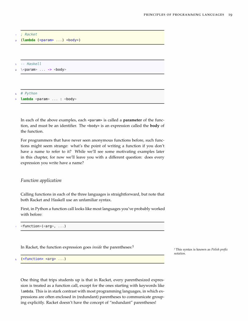
In the lambda calculus, all function function are anonymous: (λx.x) is a functionvalue, but doesn’t have an associated name. All three of Racket, Haskell, andPython support anonymous functions as well, using the following syntax, eachinspired in its own way by the lambda calculus.4
4 We’ll use background colours to dis-tinguish languages in code blocks, withyellow for Racket, blue for Haskell, andgray for all others.
principles of programming languages 19
1 ; Racket
2 (lambda (<param> ...) <body>)
1 -- Haskell
2 \<param> ... -> <body>
1 # Python
2 lambda <param> ... : <body>
In each of the above examples, each <param> is called a parameter of the func-tion, and must be an identifier. The <body> is an expression called the body ofthe function.
For programmers that have never seen anonymous functions before, such func-tions might seem strange: what’s the point of writing a function if you don’thave a name to refer to it? While we’ll see some motivating examples laterin this chapter, for now we’ll leave you with a different question: does everyexpression you write have a name?
Function application
Calling functions in each of the three languages is straightforward, but note thatboth Racket and Haskell use an unfamiliar syntax.
First, in Python a function call looks like most languages you’ve probably workedwith before:
1 <function>(<arg>, ...)
In Racket, the function expression goes inside the parentheses:55 This syntax is known as Polish prefixnotation.
1 (<function> <arg> ...)
One thing that trips students up is that in Racket, every parenthesized expres-sion is treated as a function call, except for the ones starting with keywords likelambda. This is in stark contrast with most programming languages, in which ex-pressions are often enclosed in (redundant) parentheses to communicate group-ing explicitly. Racket doesn’t have the concept of “redundant” parentheses!

20 david liu
In Haskell, parentheses are not required at all; instead, any two expressionsseparated by a space are considered a function call:
1 <function> <arg> ...
Operators are functions
Consider common binary arithmetic operations like addition and multiplication,which we normally think of as being written infix, i.e., between its two argumentexpressions: 3 + 4 or 1.5 * 10.
Again in the theme of the centrality of functions to our programming, it’s im-portant to realize that in fact, these operators are just functions, at least from amathematical point of view.6 In fact, all three of Racket, Haskell, and Python
6 Formally, we might write somethinglike + : R×R → R to represent the +operation as taking two real numbersand outputting a real number.
treat them as functions!
In Racket, operators are just identifiers that refer to built-in functions, and arecalled the same way any other function would be called:
1 > (+ 10 20)
2 30
3 > (* 3 5)
4 15
In Python, operators are implemented under the hood by delegating to various“dunder methods” for built-in classes:
1 >>> 10 + 20
2 30
3 >>> int.__add__(10, 20) # Equivalent to 10 + 20
4 30
Haskell uses a similar approach. Every infix operator (e.g., +) is a function whosename is the same as the operator, but enclosed in parentheses (e.g., (+)):
1 > 10 + 20
2 30
3 > (+) 10 20
4 30
Again, pretty weird! If you’ve never thought about it before, this might seemoverly complex. Racket actually has the cleanest model (no infix operators, uni-form prefix syntax for all functions), at the cost of being more unfamiliar; Python

principles of programming languages 21
and Haskell both include a level of indirection to support the more familiar infixsyntax we learn in mathematics.
Function purity
One thing you might notice about our grammar rules for defining functions isthat a function body is just a single expression. This is again a consequenceof our model of an expression-based language, rather than the imperative-style“sequence of statements” that you normally see in other languages.
The best way to think about functions in this style of programming is by analogythe mathematical functions, e.g. f (x) = x + 1, which are purely determined byinput-output pairs. In this definition, we say that the body of f is the expressionx + 1, and that we evaluate calls to f by substituting values for x into the body,evaluating the body expression, and then returning the result.
In the function definition rules we gave above, all the function values producedbehave exactly the same as mathematical functions: their behaviour is entirelydetermined by what their body expression evaluates to for a set of given argu-ments. For example, consider the Racket function (lambda (x) (+ x 1)). If wecall this function on the number 10,
1 ((lambda (x) (+ x 1)) 10)
we evaluate this function call by taking the 10 and substituting it for x in theexpression (+ x 1), producing 11 as the returned value. Note that a return
keyword isn’t necessary: given the lambda expression, we know precisely thatthe value of (+ x 1) (with something substituted for x) will be returned.
In programming, we say that a (mathematically) pure function is a functionthat satisfies the following properties:
1. The function’s behaviour is exactly determined by the value of its inputs. Forexample, the function cannot access data from “outside” its inputs, includingstandard input, the file system, the Internet, etc. This also rules out random-ized functions; we say that pure functions must be deterministic.
2. The function only returns a value, and does nothing else. In parallel to (1),this means that pure functions cannot print to standard output, write to thefile system, or send data across the Internet. We call such actions side effects,and so we say that “pure functions have no side effects.”
This definition might seem overly restrictive: we often want functions to com-municate with the “outside world”, either for input or output! As is hopefullybecoming a common theme in this course, we start with this type of functionbecause such functions are easiest to reason about: if you understand substitu-tion, then you’re good to go. In the final chapter of these notes, we’ll see how

22 david liu
to incorporate side effects like mutation and external I/O into a pure functionalmodel.
Name bindings
While Alonzo Church and Alan Turing showed that anonymous functions andfunction application are sufficient to perform all computations that modern pro-gramming languages can, even pure functional programming languages likeHaskell offer additional conveniences for the programmer. We’ve previouslydiscussed some of these—primitive values and built-in functions—and the fol-lowing example illustrates another:
1 (((lambda (x)
2 ((lambda (f)
3 (lambda (n)
4 (if (equal? n 0) 1 (* n (f (- n 1))))))
5 (lambda (v) ((x x) v))))
6 (lambda (x) ((lambda (f)
7 (lambda (n)
8 (if (equal? n 0) 1 (* n (f (- n 1))))))
9 (lambda (v) ((x x) v)))))
10 10)
This monstrosity of a program evaluates to 3628800, which is 10!, illustratingthe power of anonymous functions to successfully implement something of arecursive nature. However, we certainly don’t want to get stuck writing codelike this! Instead, every programming language gives us the ability to bindidentifiers to values, so that evaluating an identifier results in the value that theidentifier is bound to.
You have seen one kind of identifier already: the formal parameters used infunction definitions. These are a special type of identifier, and are bound to val-ues when the function is called. In this subsection we’ll look at using identifiersmore generally. We’ll use identifiers for two purposes:
1. To “save” the value of subexpressions so that we can refer to them later.2. To refer to a function name within the body of the function, enabling recursive
definitions.
The former is clearly just a convenience to the programmer; the latter does posea problem to us, but it turns out that writing recursive functions in the lambdacalculus is possible, as we illustrated in the above example.7
7 The main construct used to implementrecursive functions is known as the Ycombinator.It is important to keep in mind that all uses of identifiers beyond their use as
parameter names are as a convenience, to make our programs easier to under-stand, but not to truly extend the power of the lambda calculus. Unlike the

principles of programming languages 23
imperative programming languages you’ve used so far, identifier bindings inpure functional programming are immutable: once bound to a particular value,that identifier cannot be re-bound, and so literally is an alias for a value. Thisleads us to an extremely powerful concept known as referential transparency.We say that an identifier is referentially transparent if it can be substituted withits value in the source code without changing the meaning of the program.8
8 This again parallels mathematics.When we write Llet x = 5" in a state-ment or proof, any subsequent state-ment we make about x should makejust as much sense if we replace the xwith 5.
This approach to identifiers in functional programming is hugely different thanwhat we are used to in imperative programming, in which re-binding names isnot just allowed, but required for some common constructs,9 or subverted by
9 e.g., loopsmutable data structures. Given that re-binding and mutation feels so natural tous, why would we want to give it up? Or put another way, why is referentialtransparency (which is violated by mutation) so valuable?
Mutation is a powerful tool, but also makes our code harder to reason about: weneed to constantly keep track of the “current value” of every identifier through-out the execution of a program. Referential transparency means we can usenames and values interchangeably when we reason about our code regardlessof where these names appear in the program; a name, once defined, has thesame meaning for the rest of the time.10
10 In particular, the whole issue ofwhether an identifier represents a valueor a reference is rendered completelymoot.
For about 95% of this course we will not use any mutation at all, and even whenwe do use it, it will be in a very limited way. Remember that the point is to getyou thinking about programming in a different way, and we hope in fact thatthis ban will simplify your programming!
Global (aka top-level) name bindings
In Racket, the syntax for a global name binding uses the keyword define:
1 (define <id> <expr>)
In Haskell and Python, global bindings are written using the familiar = symbol:
1 <id> = <expr>
These definitions bind the value of <expr> to the identifier <id>. Here are someexamples of these bindings, including a few that bind a name to a function.
1 # Racket
2 (define a 3)
3 (define add-three
4 (lambda (x) (+ x 3)))
5
6 # Haskell
7 a = 3
24 david liu
8 addThree = \x -> x + 3
9
10 # Python
11 a = 3
12 add_three = lambda x : x + 3
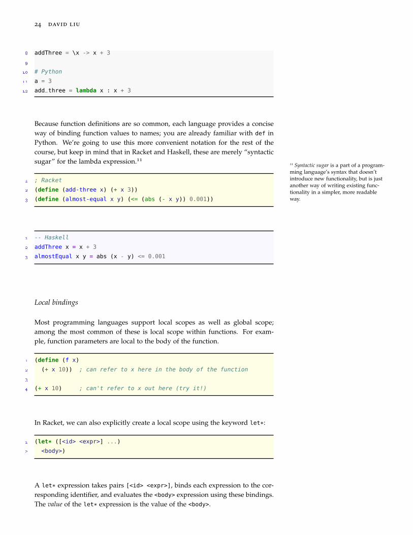
Because function definitions are so common, each language provides a conciseway of binding function values to names; you are already familiar with def inPython. We’re going to use this more convenient notation for the rest of thecourse, but keep in mind that in Racket and Haskell, these are merely “syntacticsugar” for the lambda expression.11
11 Syntactic sugar is a part of a program-ming language’s syntax that doesn’tintroduce new functionality, but is justanother way of writing existing func-tionality in a simpler, more readableway.
1 ; Racket
2 (define (add-three x) (+ x 3))
3 (define (almost-equal x y) (<= (abs (- x y)) 0.001))
1 -- Haskell
2 addThree x = x + 3
3 almostEqual x y = abs (x - y) <= 0.001
Local bindings
Most programming languages support local scopes as well as global scope;among the most common of these is local scope within functions. For exam-ple, function parameters are local to the body of the function.
1 (define (f x)
2 (+ x 10)) ; can refer to x here in the body of the function
3
4 (+ x 10) ; can't refer to x out here (try it!)
In Racket, we can also explicitly create a local scope using the keyword let*:
1 (let* ([<id> <expr>] ...)
2 <body>)
A let* expression takes pairs [<id> <expr>], binds each expression to the cor-responding identifier, and evaluates the <body> expression using these bindings.The value of the let* expression is the value of the <body>.

principles of programming languages 25
In Haskell, the same local scoping is achieved using the following:12
12 There’s one subtle difference betweenRacket’s let* and Haskell’s let: thelatter allows for recursive bindings,while the former does not. If you everneed to do this in Racket, you can useletrec instead.
1 let <id> = <expr>
2 ...
3 in
4 <body>
What about Python? Python certainly has the concept of local scope, e.g., func-tion and class definitions, but it does not have special syntactic support for letexpressions, i.e., an expression that involves local bindings and that evaluates toproduce a value. This is yet another reminder of the way in which Python isoriented around statements—assignment statements being the most common ofthese—while Racket and Haskell are oriented around expressions.
Name bindings and code structure
In the previous chapter, we said that we would focus on programs in expression-based contexts, in which a program is just a single expression to be evaluated.In practice, this is unwieldy, and this section described the use of identifiers tosimplify complex expressions. Therefore the actual program form we’ll stickwith for this course is:
1 <prog> = <binding> ... <expr>
where <binding> is a top-level binding expression. Moreover, the <expr> cannow use let expressions, which are structured in the same style: an arbitrarynumber of (distinct) name bindings, followed by a single expression to evaluate.For example, here is a Racket program that computes the distance between threedistinct points and evaluates to the minimum distance:13
13 Try writing the equivalent programwithout using any user-defined names!It’s certainly possible, but quite terribleto do so.
1 (define p1 (list 2 3))
2 (define p2 (list 10 8))
3 (define p3 (list -1 6))
4
5 (define (distance p q)
6 (let* ([dx (abs (- (first p) (first q)))]
7 [dy (abs (- (second p) (second q)))])
8 (sqrt (+ (* dx dx) (* dy dy)))))
9
10 (define distance-p1-p2 (distance p1 p2))
11 (define distance-p1-p3 (distance p1 p3))
12 (define distance-p2-p3 (distance p2 p3))
13
14 (min distance-p1-p2 distance-p1-p3 distance-p2-p3)

26 david liu
Written in Python, such a program is simply one where every global or localblock of code consists of an arbitrary number of assignments to distinct vari-ables, followed by a single expression to evaluate (or return, if inside a function).The important thing to keep in mind in that context is that such assignments arenon-mutating: we never bind to the same variable more than once!
Lists and structural recursion
The list data type is one of the most fundamental in programming languages;it is an arbitrary-length compound data type, used to store any number of val-ues.14 For many of us, lists are the first time we are able to write code that
14 In fact, the name “Lisp” comes from“list processing.”operates on an arbitrary amount of data, without knowing ahead of time how
much data there is.
Imperative languages naturally process lists using loops, explicitly relying onnotions of time and state to keep track of the “current” list element. This followsa metaphor of a list as a linear sequence of items, in which each item is “pro-cessed” one at a time. However, because pure functional programming does notpermit the mutation required to re-bind an identifier to each element of the listin turn, we must take another approach to writing programs involving lists.
The key insight here is to identify a recursive structure for the list data type, anduse this definition to inform both our representation of and operations on lists.A list is defined recursively as:
• The empty list is a list. (Represented in Racket as '(), in Haskell and Pythonas [].)
• If x is a value and lst is a list, then we can create a new list whose first elementis x and whose other items are the ones from lst. We call this combinationthe cons operation,15 calling the produced list “x cons lst.” In Racket, this is
15 short for “construct”represented by the cons function, and in Haskell by the infix operator (:).16
16 Python doesn’t have a built-in func-tion that does this, perhaps evidencethat this recursive representation is notcentral to Python lists (which it isn’t).
For example, we could construct the list [1, 2, 3] using this recursive defini-tion in Racket as (cons 1 (cons 2 (cons 3 '()))), and in Haskell as 1:2:3:[].In Racket and Haskell, we can deconstruct non-empty lists into their first andother elements, by using functions first and rest (Racket), or head and tail
(Haskell). We have the identity lst = (cons (first lst) (rest lst)) for allnon-empty lists lst.
Structural recursion on lists
This recursive structure informs not just how we represent lists, but how weoperate on lists as well. For example, consider the problem of computing thesum of the elements of a list. Whereas an iterative approach would process eachelement in turn by adding its value to an accumulator, a recursive approachmimics the recursive structure of the list itself:

principles of programming languages 27
• The sum of an empty list is equal to 0.• The sum of “x cons lst” is equal to x plus the sum of lst.
The beauty of this English description is that it translates immediately into apure function:
1 ; Racket
2 (define (sum lst)
3 (if (empty? lst)
4 0
5 (+ (first lst)
6 (sum (rest lst)))))
1 -- Haskell
2 sum lst =
3 if null lst
4 then
5 0
6 else
7 head lst + sum (tail lst)
And here is a function that takes a list, and returns a new list containing just themultiples of three in that list. Note that this is a filtering operation, somethingwe’ll return to later in this chapter.
1 (define (multiples-of-3 lst)
2 (cond [(empty? lst) '()]
3 [(equal? 0 (remainder (first lst) 3))
4 (cons (first lst)
5 (multiples-of-3 (rest lst)))]
6 [else (multiples-of-3 (rest lst))]))
This form of recursion is called structural recursion because the code follows thestructure of the data type on which it operates. What’s remarkable about thistechnique is that because it is based solely on the form of the input data, we canapply it to create a “code template” that works for many list functions:
1 (define (f lst)
2 (if (empty? lst)
3 ...
4 (... (first lst)
5 (f (rest lst)))))

28 david liu
Moreover, this technique can be used for any data type with a recursive defi-nition, not just lists. The other fundamental example we’ll return to again andagain in this course is the recursive definition of trees, and specifically the ab-stract syntax trees that we use to represent programs.
Exercise Break!
The following programming exercises are meant to give you practice workingwith structural recursion on lists. We recommend completing them in bothRacket and Haskell.
1.1 Write a function to determine the length of a list.
1.2 Write a function to determine if a given item appears in a list.
1.3 Write a function to determine the number of duplicates in a list.
1.4 Write a function to remove all duplicates from a list.
1.5 Given two lists, output the items that appear in both lists (intersection). Then,output the items that appear in at least one of the two lists (union).
1.6 Write a function that takes a list of lists, and returns the list that contains thelargest item (e.g., given (list (list 1 2 3) (list 45 10) (list) (list 15)),return (list 45 10).
1.7 Write a function that takes an item and a list of lists, and inserts the item atthe front of every list.
1.8 Write a function that takes a list with no duplicates representing a set (orderdoesn’t matter), and returns a list of lists containing all of its subsets.
1.9 Write a function that takes a list with no duplicates, and a number k, andreturns all subsets of size k of that list.
1.10 (Racket only) Modify your function to the previous question so that the pa-rameter k is optional, and if not specified, the function returns all subsets.
1.11 Write a function that takes a list, and returns all permutations of that list.
1.12 A sublist of a list is a series of consecutive items of the list. Given a list ofnumbers, find the maximum sum of any sublist of that list. (Note: there is aO(n) algorithm that does this, although you should try to get any algorithmthat is correct first, as the O(n) algorithm is a little more complex.)
Pattern-matching
We’ll now take a short detour away from the pure lambda calculus to introduceone of the most underutilized programming language features: pattern-matching,which allows the programmer to specify conditional behaviour depending onthe structure of a given value in a concise and understandable syntax. As anexample, consider the following value-based branching function definition:

principles of programming languages 29
1 f x =
2 if x == 0
3 then
4 10
5 else if x == 1
6 then
7 20
8 else
9 x + 30
While this is fine, we can shorten this substantially in Haskell by using valuepattern-matching in the function definition.17 Rather than giving one generic
17 Here, we’ll focus on pattern-matchingfor function definitions only, althoughboth Racket and Haskell supportpattern-matching as an arbitrary ex-pression form as well.
function signature f x = ..., we give three pattern-based definitions:
1 f 0 = 10
2 f 1 = 20
3 f x = x + 30
Essentially, Haskell’s function definition syntax allows us to eliminate the ex-plicit use of if-else tests; instead, we provide the patterns (in this case, 0, 1,or x—an identifier matches anything18) and the Haskell compiler generates the
18 Order matters! The patterns arechecked top-down, with the first matchbeing selected.
equivalent code that does the testing for us whenever this function is called.
Here is the same idea expressed in Racket. The syntax isn’t quite as terse (notethe use of the define/match keyword), but is certainly more concise than usingifs or even cond:
1 (define/match (f x)
2 [(0) 10]
3 [(1) 20]
4 [(_) (+ x 30)]) ; The underscore matches anything
While the above example is cute, you might be skeptical that it generalizes; afterall, how often do we write explicit special cases when defining functions? But itturns out that pattern-matching goes far beyond simple value-equality checks.Consider now this recursive list function from the previous section, which wegeneralized into a template for structural recursion on lists.
1 (define (sum lst)
2 (if (empty? lst)
3 0
4 (+ (first lst)
5 (sum (rest lst)))))
30 david liu
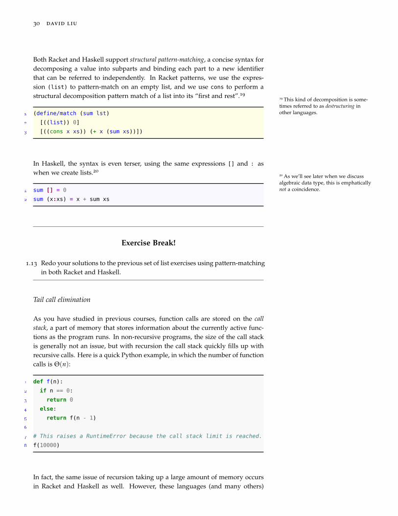
Both Racket and Haskell support structural pattern-matching, a concise syntax fordecomposing a value into subparts and binding each part to a new identifierthat can be referred to independently. In Racket patterns, we use the expres-sion (list) to pattern-match on an empty list, and we use cons to perform astructural decomposition pattern match of a list into its “first and rest”.19
19 This kind of decomposition is some-times referred to as destructuring inother languages.1 (define/match (sum lst)
2 [((list)) 0]
3 [((cons x xs)) (+ x (sum xs))])
In Haskell, the syntax is even terser, using the same expressions [] and : aswhen we create lists.20
20 As we’ll see later when we discussalgebraic data type, this is emphaticallynot a coincidence.1 sum [] = 0
2 sum (x:xs) = x + sum xs
Exercise Break!
1.13 Redo your solutions to the previous set of list exercises using pattern-matchingin both Racket and Haskell.
Tail call elimination
As you have studied in previous courses, function calls are stored on the callstack, a part of memory that stores information about the currently active func-tions as the program runs. In non-recursive programs, the size of the call stackis generally not an issue, but with recursion the call stack quickly fills up withrecursive calls. Here is a quick Python example, in which the number of functioncalls is Θ(n):
1 def f(n):
2 if n == 0:
3 return 0
4 else:
5 return f(n - 1)
6
7 # This raises a RuntimeError because the call stack limit is reached.
8 f(10000)
In fact, the same issue of recursion taking up a large amount of memory occursin Racket and Haskell as well. However, these languages (and many others)

principles of programming languages 31
perform tail call elimination, which can significantly reduce the space require-ments for recursive functions. A tail call is a function call that happens as thelast instruction of a function before the return; the f(n-1) call in the previousexample has this property. When a tail call occurs, there is no need to rememberwhere it was called from, because the only thing that’s going to happen after-wards is that the value will be returned to the original caller.21 This property of
21 Simply put: if f calls g and g just callsh and returns its value, then when h
is called there is no need to keep anyinformation about g; just return thevalue to f directly!
tail calls is common to all languages; however, some languages take advantageof this, and others do not. Racket is one that does: when it calls a function thatit detects is in tail call position, it first removes the calling function’s stack framefrom the call stack, leading to constant stack height for this:
1 (define (f n)
2 (if (equal? n 0)
3 0
4 (f (- n 1))))
Transforming simple recursive functions into tail-recursive ones
Now let’s return our our sum implementation from the previous section:
1 (define (sum lst)
2 (if (empty? lst)
3 0
4 (+ (first lst)
5 (sum (rest lst)))))
This implementation is not tail-recursive! In the “else” expression, it is the +,not sum, that is called in tail position. The sum call is enclosed inside the outerfunction call (+ (first lst) _): after the recursive sum call returns, its result isadded to (first lst) before being returned.22
22 The notation (+ (first lst) _)
captures the idea of a continuation thatwe’ll study in more detail in the nextchapter.
In this case, there is a natural way to convert this sum implementation into onethat is tail-recursive by essentially replacing the (+ (first lst) _) with a singlerecursive call. To do this, we use an extra accumulating parameter to store the“add (first lst)” part, updating its value at each recursive call. Here is ourtail-recursive implementation:
1 (define (sum-tail lst)
2 (sum-helper lst 0))
3
4 (define (sum-helper lst acc)
5 (if (empty? lst)
6 acc
7 (sum-helper (rest lst) (+ acc (first lst)))))

32 david liu
In the above example, the parameter acc plays this role, accumulating the sumof the items “processed so far” in the list. We can use substitution to see exactlywhat happens when we call (sum-tail '(1 2 3 4)):
1 (sum-tail '(1 2 3 4))
2 (sum-helper '(1 2 3 4) 0) ; Initial call to sum-helper; acc = 0
3 (sum-helper '(2 3 4) 1) ; The new acc value is
4 ; (+ 0 (first '(1 2 3 4))) = = 1
5 (sum-helper '(3 4) 3) ; acc = (+ 1 (first '(2 3 4))) = 3
6 (sum-helper '(4) 6) ; acc = (+ 3 (first '(3 4))) = 6
7 (sum-helper '() 10) ; acc = (+ 6 (first '(4))) = 10
8 10 ; Base case: acc is returned
As you might expect, this transformation technique generalized beyond this sim-ple example! For example, here is the exact same idea applied to our earliermultiples-of-3 function:23
23 Question: Why did we use append
and not cons here?
1 (define (multiples-of-3 lst)
2 (multiples-of-3-helper lst '()))
3
4 (define (multiples-of-3-helper lst acc)
5 (if (empty? lst)
6 acc
7 (multiples-of-3-helper (rest lst)
8 (if (equal? 0 (remainder (first lst) 3))
9 (append acc (list (first lst)))
10 acc))))
Exercise Break!
1.14 Rewrite your solutions to the previous exercises using tail recursion.
1.15 Consider a generalized version of the standard recursive template:
1 (define (f lst)
2 (if (empty? lst)
3 x
4 (g (first lst) (f (rest lst)))))
(Here, x and g are arbitrary.) Transform f into an equivalent tail-recursivefunction.

principles of programming languages 33
From tail recursion to loops
Let’s look once more at sum-tail:
1 (define (sum-tail lst)
2 (sum-helper lst 0))
3
4 (define (sum-helper lst acc)
5 (if (empty? lst)
6 acc
7 (sum-helper (rest lst) (+ acc (first lst)))))
Our previous trace through the evaluation of (sum-tail '(1 2 3 4)) producedthe function calls (sum-helper '(1 2 3 4) 0), (sum-helper '(2 3 4) 1), etc.In a language without tail call elimination, all of these sum-helper calls wouldoccupy separate frames on the stack, but in a language (like Racket) that per-forms tail call elimination, we know that each of these function calls replaces thestack frame for the one before it. In particular, we can view the sequence
1 (sum-helper '(1 2 3 4) 0)
2 (sum-helper '(2 3 4) 1)
3 (sum-helper '(3 4) 3)
4 (sum-helper '(4) 6)
5 (sum-helper '() 10)
not as five separate function calls, but instead five separate executions of thefunction body, with the argument values lst and acc changing at each iteration.And of course, repeated executions of a block of code is naturally representedin an iterative manner using loops.
To see this transformation in action, we first write our existing code in Python:24
24 Note that while Python does notperform tail-call elimination, that’s animplementation detail—the algorithmremains unchanged.
1 def sum_tail(main_lst):
2 return sum_helper(main_lst, 0)
3
4 def sum_helper(lst, acc):
5 if lst == []:
6 return acc
7 else:
8 # The lst[1:] implements (rest lst), but is unidiomatic Python.
9 return sum_helper(lst[1:], acc + lst[0])
We now will transform sum_helper into a while loop as follows:
• Initialize two variables lst and acc representing the parameters of sum_helper,

34 david liu
using the argument values in the initial call sum_helper(main_lst, 0).• Place the body of sum_helper inside a while True loop.• Replace the recursive sum_helper call with statements to update the values of
lst and acc.
Applying these rules gives us the resulting code:
1 def sum_tail2(main_lst):
2 lst, acc = main_lst, 0
3
4 while True:
5 if lst == []:
6 return acc
7 else:
8 lst, acc = lst[1:], acc + lst[0]
Now, this code is certainly unidiomatic Python code, both because of the while
True and because of the list slicing operation lst[1:]. The beauty of this ap-proach is that we obtained this code by applying a mechanical transformation onour tail-recursive version—that is, without taking into account anything aboutthe tail-recursive function did! Further analysis on our part would reveal that thelst == [] and lst = lst[1:] pieces act as boilerplate to iterate through eachelement of the list main_lst, and so we can simplify this to the very idiomatic
1 def sum_tail3(main_lst):
2 acc = 0
3 for x in main_lst:
4 acc = acc + x
5 return acc
Exercise Break!
1.16 Consider a Python function of the following form:
1 def f(main_lst):
2 lst, acc = main_lst, 0
3
4 while True:
5 if lst == []:
6 return g1(acc)
7 else:
8 lst, acc = lst[1:], g2(lst[0], acc)

principles of programming languages 35
Rewrite this function into idiomatic Python, in the same way we did forsum_tail3. Make sure you understand exactly what mechanical steps youneed to perform!
Higher-order functions
So far, we have kept a strict division between our types representing data values—numbers, booleans, strings, and lists—and the functions that operate on them.However, as we said earlier, functions are values, so it is natural to ask: canfunctions operate on other functions?
The answer in our course is a most emphatic yes, and in fact this is the heartof functional programming: the ability for functions to take in other functionsand use them, combine them, and even return new ones. Let’s see some simpleprogramming examples.25
25 The differential operator, which takesas input a function f (x) and returnsits derivative f ′(x), is another exampleof a “higher-order function” (althoughmost calculus courses won’t use thisterminology). By the way, so is theindefinite integral.
1 ; Take an input *function* and apply it to 1
2 (define (apply-to-1 f) (f 1))
3 (apply-to-1 even?) ; #f
4 (apply-to-1 list) ; '(1)
5 (apply-to-1 (lambda (x) (+ 15 x))) ; 16
6
7 ; Take two functions and apply them to the same argument
8 (define (apply-two f1 f2 x)
9 (list (f1 x) (f2 x)))
10 (apply-two even? odd? 16) ; '(#t #f)
11
12 ; Apply the same function to an argument twice in a row
13 (define (apply-twice f x)
14 (f (f x)))
15 (apply-twice sqr 3) ; 81
Higher-order list functions
With the discussion in the previous section, you might get the impression thatpeople who use functional programming spend all of their time using recursion.But in fact this is not the case! Instead of using recursion explicitly, code oftenuses three critical higher-order functions to compute with lists.26 The first two,
26 Of course, these higher-order func-tions themselves are implementedrecursively.
map and filter are extremely straightforward:
1 ; (map f lst)
2 ; Returns a new list by applying `f` to each element in `lst`
3 > (map (lambda (x) (* x 3)) (list 1 2 3 4))
4 '(3 6 9 12)
5
36 david liu
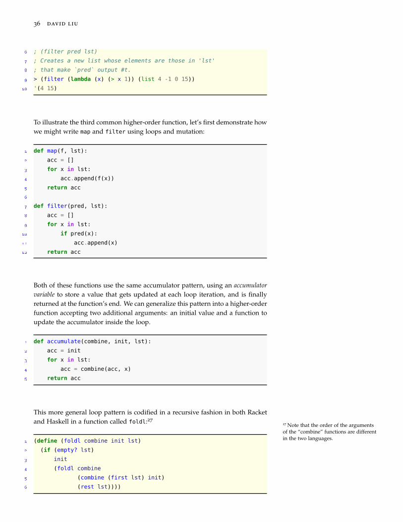
6 ; (filter pred lst)
7 ; Creates a new list whose elements are those in 'lst'
8 ; that make `pred` output #t.
9 > (filter (lambda (x) (> x 1)) (list 4 -1 0 15))
10 '(4 15)
To illustrate the third common higher-order function, let’s first demonstrate howwe might write map and filter using loops and mutation:
1 def map(f, lst):
2 acc = []
3 for x in lst:
4 acc.append(f(x))
5 return acc
6
7 def filter(pred, lst):
8 acc = []
9 for x in lst:
10 if pred(x):
11 acc.append(x)
12 return acc
Both of these functions use the same accumulator pattern, using an accumulatorvariable to store a value that gets updated at each loop iteration, and is finallyreturned at the function’s end. We can generalize this pattern into a higher-orderfunction accepting two additional arguments: an initial value and a function toupdate the accumulator inside the loop.
1 def accumulate(combine, init, lst):
2 acc = init
3 for x in lst:
4 acc = combine(acc, x)
5 return acc
This more general loop pattern is codified in a recursive fashion in both Racketand Haskell in a function called foldl:27
27 Note that the order of the argumentsof the “combine” functions are differentin the two languages.
1 (define (foldl combine init lst)
2 (if (empty? lst)
3 init
4 (foldl combine
5 (combine (first lst) init)
6 (rest lst))))
principles of programming languages 37
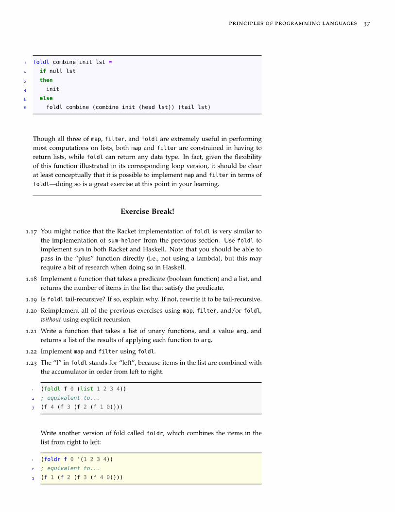
1 foldl combine init lst =
2 if null lst
3 then
4 init
5 else
6 foldl combine (combine init (head lst)) (tail lst)
Though all three of map, filter, and foldl are extremely useful in performingmost computations on lists, both map and filter are constrained in having toreturn lists, while foldl can return any data type. In fact, given the flexibilityof this function illustrated in its corresponding loop version, it should be clearat least conceptually that it is possible to implement map and filter in terms offoldl—doing so is a great exercise at this point in your learning.
Exercise Break!
1.17 You might notice that the Racket implementation of foldl is very similar tothe implementation of sum-helper from the previous section. Use foldl toimplement sum in both Racket and Haskell. Note that you should be able topass in the “plus” function directly (i.e., not using a lambda), but this mayrequire a bit of research when doing so in Haskell.
1.18 Implement a function that takes a predicate (boolean function) and a list, andreturns the number of items in the list that satisfy the predicate.
1.19 Is foldl tail-recursive? If so, explain why. If not, rewrite it to be tail-recursive.
1.20 Reimplement all of the previous exercises using map, filter, and/or foldl,without using explicit recursion.
1.21 Write a function that takes a list of unary functions, and a value arg, andreturns a list of the results of applying each function to arg.
1.22 Implement map and filter using foldl.
1.23 The “l” in foldl stands for “left”, because items in the list are combined withthe accumulator in order from left to right.
1 (foldl f 0 (list 1 2 3 4))
2 ; equivalent to...
3 (f 4 (f 3 (f 2 (f 1 0))))
Write another version of fold called foldr, which combines the items in thelist from right to left:
1 (foldr f 0 '(1 2 3 4))
2 ; equivalent to...
3 (f 1 (f 2 (f 3 (f 4 0))))
38 david liu
Hint: this can be done using basic structural recursion—start by mentallydividing the input list into first and rest.
Currying
Currying is a powerful feature of functional programming languages that allowsa function to be applied to only some of its arguments. We’ll talk more aboutcurrying when we discuss Haskell’s static type system, but for now our interestis in how currying simplifies functions whose bodies call higher-order functions.
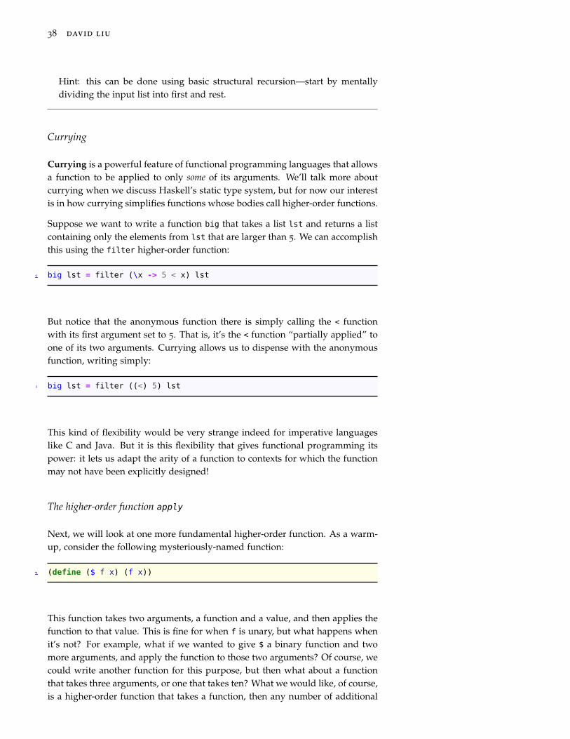
Suppose we want to write a function big that takes a list lst and returns a listcontaining only the elements from lst that are larger than 5. We can accomplishthis using the filter higher-order function:
1 big lst = filter (\x -> 5 < x) lst
But notice that the anonymous function there is simply calling the < functionwith its first argument set to 5. That is, it’s the < function “partially applied” toone of its two arguments. Currying allows us to dispense with the anonymousfunction, writing simply:
1 big lst = filter ((<) 5) lst
This kind of flexibility would be very strange indeed for imperative languageslike C and Java. But it is this flexibility that gives functional programming itspower: it lets us adapt the arity of a function to contexts for which the functionmay not have been explicitly designed!
The higher-order function apply
Next, we will look at one more fundamental higher-order function. As a warm-up, consider the following mysteriously-named function:
1 (define ($ f x) (f x))
This function takes two arguments, a function and a value, and then applies thefunction to that value. This is fine for when f is unary, but what happens whenit’s not? For example, what if we wanted to give $ a binary function and twomore arguments, and apply the function to those two arguments? Of course, wecould write another function for this purpose, but then what about a functionthat takes three arguments, or one that takes ten? What we would like, of course,is a higher-order function that takes a function, then any number of additional

principles of programming languages 39
arguments, and applies that function to those extra arguments. In Racket, wehave a built-in function called apply that does almost this:
1 ; (apply f lst)
2 ; Call f with arguments taken from the elements of lst
3 (apply + (list 1 2 3 4))
4 ; equivalent to...
5 (+ 1 2 3 4)
6
7 ; More generally,
8 (apply f (list x1 x2 x3 ... xn))
9 ; equivalent to...
10 (f x1 x2 x3 ... xn)
Note that apply differs from map, even though the types of their argumentsare very similar (both take a function and a list). Remember that map calls itsfunction argument once for each value in the list separately, while apply calls itsfunction argument just once, on all of the items in the list at once. The returnvalue of map is always a list; the return value of apply is whatever its functionargument returns.
In Haskell, the story is similar but not identical. We have a binary infix operator($), which acts as unary function application:
1 f $ x
2 -- equivalent to...
3 f x
However, due to constraints imposed by Haskell’s type system, it does not pro-vide an equivalent to Racket’s apply, which works on functions of arbitrary arity.We’ll discuss Haskell’s type system in detail later in this course.
Exercise Break!
1.24 Look up rest arguments in Racket, which allow you to define functions thattake in an arbitrary number of arguments. Then, implement a function ($$ f
x1 ... xn), which is equivalent to (f x1 ... xn).
Functions returning functions
We have now seen functions that take primitive values and other functions, butso far they have all had primitive values as their output. Now, we’ll turn ourattention to another type of higher-order function: a function that returns a func-tion. This is extremely powerful: in its most general form, it allows us to define

40 david liu
new functions dynamically, that is, during the execution of a program. Here isa simple example of this:
1 (define (make-adder x)
2 ; The body of make-adder is a function value.
3 (lambda (y) (+ x y)))
4 (make-adder 10) ; #<procedure>
5
6 (define add-10 (make-adder 10))
7 add-10 ; #<procedure>
8 (add-10 3) ; 13
The function add-10 certainly seems to be adding ten to its argument; using thesubstitution model of evaluation for (make-adder 10), we see how this happens:
1 (make-adder 10)
2 ; ==> (substitute 10 for x in the body of make-adder)
3 (lambda (y) (+ 10 y))
Exercise Break!
1.25 Write a function that takes a single argument x, and returns a new functionthat takes a list and checks whether x is in that list or not.
1.26 Write a function that takes a unary function and a positive integer n, andreturns a new unary function that applies the function to its argument ntimes.
1.27 Write a function flip that takes a binary function f, and returns a new binaryfunction g such that (g x y) = (f y x) for all valid arguments x and y.
1.28 Write a function that takes two unary functions f and g, and returns a newunary function that always returns the max of f and g applied to its argument.
1.29 Write the following Racket function:
1 #|
2 (fix f n x)
3 f: a function taking m arguments
4 n: a natural number, 1 <= n <= m
5 x: an argument
6
7 Return a new function g that takes m-1 arguments,
8 which acts as follows:
9 (g a_1 ... a_{n-1} a_{n+1} ... a_m)
10 = (f a_1 ... a_{n-1} x a_{n+1} ... a_m)
11
principles of programming languages 41
12 That is, x is inserted as the nth argument in a call to f.
13
14 > (define f (lambda (x y z) (+ x (* y (+ z 1)))))
15 > (define g (fix f 2 100))
16 > (g 2 4) ; equivalent to (f 2 100 4)
17 502
18 |#
(Hint: recall rest arguments from an earlier exercise.)
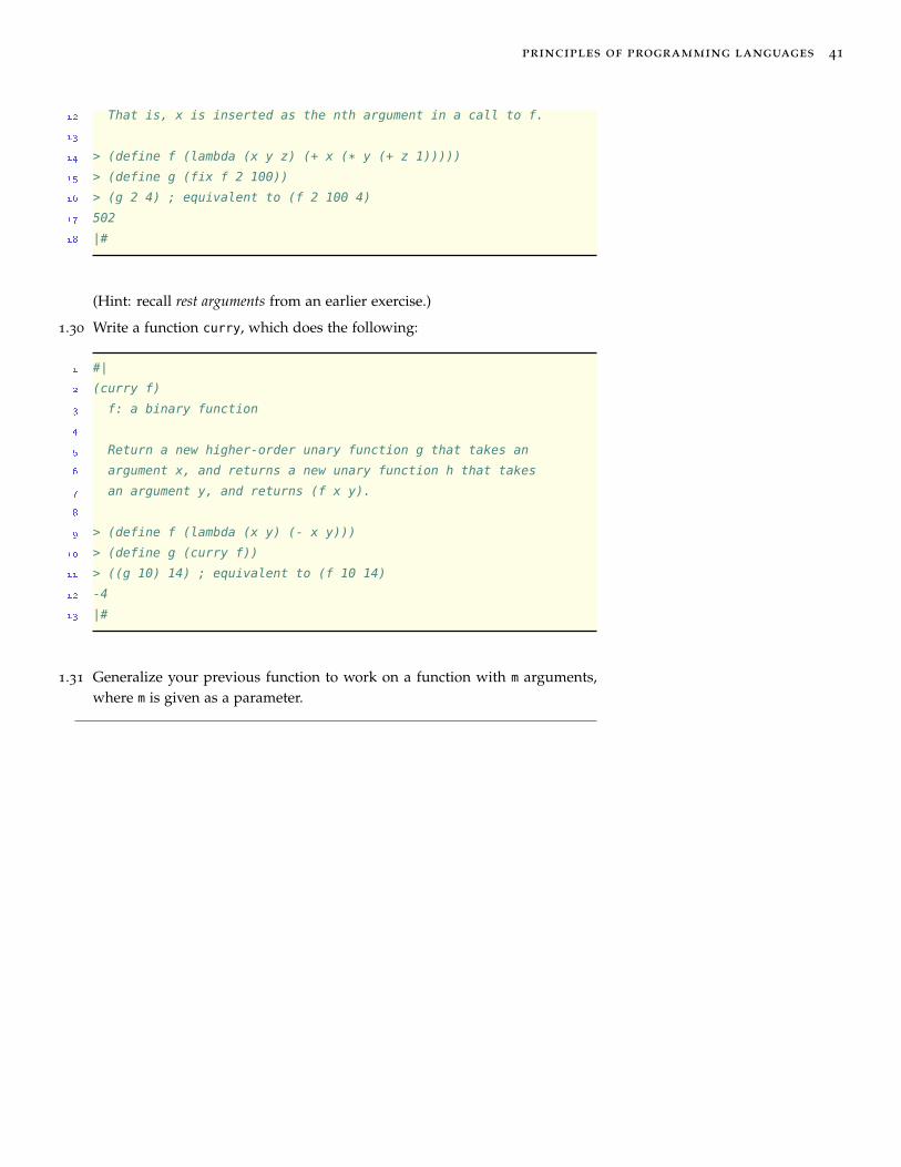
1.30 Write a function curry, which does the following:
1 #|
2 (curry f)
3 f: a binary function
4
5 Return a new higher-order unary function g that takes an
6 argument x, and returns a new unary function h that takes
7 an argument y, and returns (f x y).
8
9 > (define f (lambda (x y) (- x y)))
10 > (define g (curry f))
11 > ((g 10) 14) ; equivalent to (f 10 14)
12 -4
13 |#
1.31 Generalize your previous function to work on a function with m arguments,where m is given as a parameter.

42 david liu
Programming with abstract syntax trees
A natural generalization of the list data type is the tree data type, in whichthe “recursive” part contains an arbitrary number of recursive subcomponentsrather than just one. In this section, we’ll start looking at how abstract syntaxtrees (ASTs) are represented in real code, and how our discussion of structuralrecursion allows us to easily operate on such trees.
Racket: Quoted expressions
First, let’s see how we can represent ASTs in Racket. This is actually one ofthe fundamental strengths of all Lisp languages: the parenthesization of thesource code immediately creates a nested list structure, which is simply anotherrepresentation of a tree. To make this even more explicit in the language, anyRacket expression (no matter how complex or deeply nested) can be turnedinto a static nested list simply by prefixing it with an apostrophe. We call thisquoting an expression.
1 > (+ 1 2) ; A regular Racket expression
2 3
3 > '(+ 1 2) ; Quoting the expression: a list of three elements.
4 '(+ 1 2)
5 > (first '(+ 1 2))
6 '+
7 > (second '(+ 1 2))
8 1
9 > (third '(+ 1 2))
10 2
11 > '(+ (* 2 3) (* 4 5)) ; This is a nested list
12 '(+ (* 2 3) (* 4 5))
Even though in Racket a quoted expression really is just a list, we will call it aRacket datum28 to distinguish it from a regular list. Formally, here are the types
28 plural: “datums”, not “data” to avoidconfusionof values that comprise the “tree” in a Racket datum:
1. Quoted literals (5, #t, "hello") represent those same values as in the originalcode: for example, (equal? '5 5) returns true.
2. Quoted identifiers and keywords become symbols; a symbol is a primitivedatatype that functions as a unique identifier. For example, the datum '(+
1 2) has as its first element the symbol '+, which can be compared usingequal? to other values, and used in pattern-matching. Note that keywordslike define also get quoted into symbols, and so the only way to determinewhich symbols correspond to identifiers and which correspond to keywordsis to start with a fixed set of keywords to check.
3. Quoted compound expressions become lists, in which each element is thequoted version of the corresponding subexpression. '(+ 2 3) is equivalent

principles of programming languages 43
to (list '+ '2 '3), which is in turn equivalent to (list '+ 2 3).
Given this structure, we can use structural pattern-matching to take in a datumand perform recursive computations on it. For example, here is a function thattakes a Racket datum consisting of just numeric literals, identifiers, and arith-metic function calls, and returns the number of times + is used:
1 (define/match (num-plus datum)
2 ; For a function call (which in this case is *any* parenthesized
3 ; expression), recurse on each subexpression and add up the total
4 ; number of occurrences. Note the use of (list expr ...) to bind
5 ; lists of arbitrary length to expr.
6 [((list expr ...))
7 (apply + (map num-plus expr))]
8 ; Value pattern-match on '+
9 [('+) 1]
10 ; For any other atomic value (identifier or literal), return 0
11 [(_) 0])
12
13 > (num-plus '+)
14 1
15 > (num-plus 3)
16 0
17 > (num-plus '(+ (* 4 5) (+ (- (+ 3 6) 7) 8)))
18 3
Haskell: value constructors
As a consequence of Haskell’s type system, we cannot store values of differ-ent types in the same list, making it cumbersome to directly represent Racketdatums in the same way (note that those Racket lists freely mix nested lists,symbols, and literals of all different types). Instead, Haskell’s type system per-mits the concise declaration of, and pattern-matching on, a type with multipledifferent constructors. We will study this more formally later in the course, butfor now we think you’ll find the following representation of an “expression”type to be quite intuitive:
1 data Expr = NumLiteral Int -- An integer literal
2 | Identifier String -- An identifier
3 | Call Expr [Expr] -- A function call, where the first
4 -- Expr is the function being called,
5 -- and the list [Expr] contains the
6 -- argument expressions.
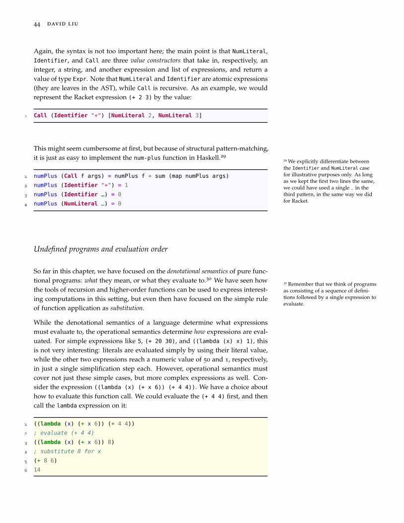
44 david liu
Again, the syntax is not too important here; the main point is that NumLiteral,Identifier, and Call are three value constructors that take in, respectively, aninteger, a string, and another expression and list of expressions, and return avalue of type Expr. Note that NumLiteral and Identifier are atomic expressions(they are leaves in the AST), while Call is recursive. As an example, we wouldrepresent the Racket expression (+ 2 3) by the value:
1 Call (Identifier "+") [NumLiteral 2, NumLiteral 3]
This might seem cumbersome at first, but because of structural pattern-matching,it is just as easy to implement the num-plus function in Haskell.29
29 We explicitly differentiate betweenthe Identifier and NumLiteral casefor illustrative purposes only. As longas we kept the first two lines the same,we could have used a single _ in thethird pattern, in the same way we didfor Racket.
1 numPlus (Call f args) = numPlus f + sum (map numPlus args)
2 numPlus (Identifier "+") = 1
3 numPlus (Identifier _) = 0
4 numPlus (NumLiteral _) = 0
Undefined programs and evaluation order
So far in this chapter, we have focused on the denotational semantics of pure func-tional programs: what they mean, or what they evaluate to.30 We have seen how
30 Remember that we think of programsas consisting of a sequence of defini-tions followed by a single expression toevaluate.
the tools of recursion and higher-order functions can be used to express interest-ing computations in this setting, but even then have focused on the simple ruleof function application as substitution.
While the denotational semantics of a language determine what expressionsmust evaluate to, the operational semantics determine how expressions are eval-uated. For simple expressions like 5, (+ 20 30), and ((lambda (x) x) 1), thisis not very interesting: literals are evaluated simply by using their literal value,while the other two expressions reach a numeric value of 50 and 1, respectively,in just a single simplification step each. However, operational semantics mustcover not just these simple cases, but more complex expressions as well. Con-sider the expression ((lambda (x) (+ x 6)) (+ 4 4)). We have a choice abouthow to evaluate this function call. We could evaluate the (+ 4 4) first, and thencall the lambda expression on it:
1 ((lambda (x) (+ x 6)) (+ 4 4))
2 ; evaluate (+ 4 4)
3 ((lambda (x) (+ x 6)) 8)
4 ; substitute 8 for x
5 (+ 8 6)
6 14
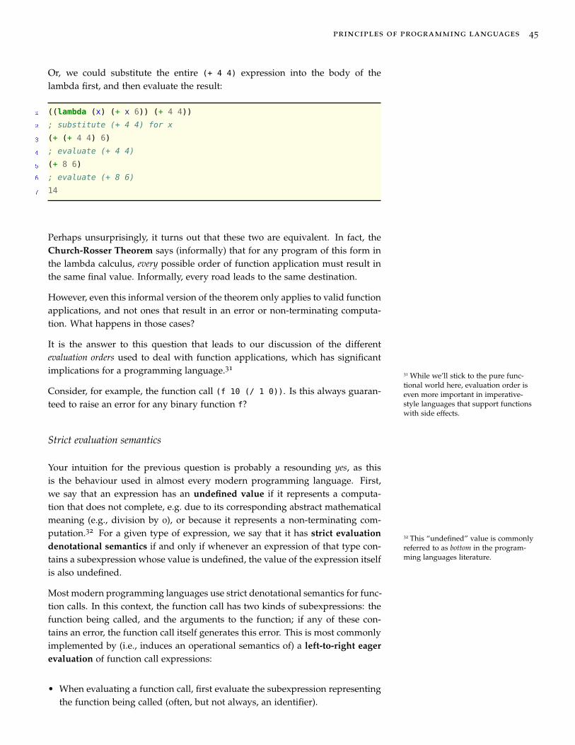
principles of programming languages 45
Or, we could substitute the entire (+ 4 4) expression into the body of thelambda first, and then evaluate the result:
1 ((lambda (x) (+ x 6)) (+ 4 4))
2 ; substitute (+ 4 4) for x
3 (+ (+ 4 4) 6)
4 ; evaluate (+ 4 4)
5 (+ 8 6)
6 ; evaluate (+ 8 6)
7 14
Perhaps unsurprisingly, it turns out that these two are equivalent. In fact, theChurch-Rosser Theorem says (informally) that for any program of this form inthe lambda calculus, every possible order of function application must result inthe same final value. Informally, every road leads to the same destination.
However, even this informal version of the theorem only applies to valid functionapplications, and not ones that result in an error or non-terminating computa-tion. What happens in those cases?
It is the answer to this question that leads to our discussion of the differentevaluation orders used to deal with function applications, which has significantimplications for a programming language.31
31 While we’ll stick to the pure func-tional world here, evaluation order iseven more important in imperative-style languages that support functionswith side effects.
Consider, for example, the function call (f 10 (/ 1 0)). Is this always guaran-teed to raise an error for any binary function f?
Strict evaluation semantics
Your intuition for the previous question is probably a resounding yes, as thisis the behaviour used in almost every modern programming language. First,we say that an expression has an undefined value if it represents a computa-tion that does not complete, e.g. due to its corresponding abstract mathematicalmeaning (e.g., division by 0), or because it represents a non-terminating com-putation.32 For a given type of expression, we say that it has strict evaluation
32 This “undefined” value is commonlyreferred to as bottom in the program-ming languages literature.
denotational semantics if and only if whenever an expression of that type con-tains a subexpression whose value is undefined, the value of the expression itselfis also undefined.
Most modern programming languages use strict denotational semantics for func-tion calls. In this context, the function call has two kinds of subexpressions: thefunction being called, and the arguments to the function; if any of these con-tains an error, the function call itself generates this error. This is most commonlyimplemented by (i.e., induces an operational semantics of) a left-to-right eagerevaluation of function call expressions:
• When evaluating a function call, first evaluate the subexpression representingthe function being called (often, but not always, an identifier).

46 david liu
• Then evaluate each argument subexpression, in left-to-right order.• Finally, “call” the function by substituting the value of each subexpression into
the body of the function.
Because arguments are evaluated before being substituted into the body of afunction, this guarantees that if one of the argument subexpressions (or even thefunction subexpression itself) is undefined, this is discovered before the functionis actually called.
Similarly, most languages use strict semantics for name bindings; for example, inRacket the top-level binding (define <id> <expr>) first evaluates <expr>, andthen binds the value of that expression to the <id>.33
33 In introductory classes, we normallylearn this as “first evaluate the right-hand side of the =, then assign the valueto the left-hand side.”Non-strict syntactic forms
In your programming experience so far, you have probably taken for grantedeager evaluation order in function calls. However, you also learned that thereare certain types of expressions that do not eagerly evaluate all of their subex-pressions, for example, boolean operators and conditionals. In Racket, these areand, or, if, and cond; even though these may look like ordinary functions, theyaren’t! Suppose we wrote our own “and” function by wrapping the built-inRacket and: (define (my-and x y) (and x y)).
Even though my-and looks identical to and, it’s not, all because of evaluation or-der. Whereas the built-in and can stop evaluating its arguments when it reachesa “false” value, the same is not true of my-and—the latter is a function, and soeagerly evaluates all of its arguments before passing their values to and:
1 (and #f (/ 1 0)) ; evaluates to #f
2 (my-and #f (/ 1 0)) ; raises an error
Because of this, we say that and, or, if, and cond are syntactic forms, rather thanidentifiers that refer to built-in functions. This point is actually rather subtle, andin fact is not specific to Racket at all! In any programming language that uses ea-ger evaluation for functions, short-circuiting boolean operations and conditionalare all implemented as syntactic constructs, not simple function calls.
Function bodies and delaying evaluation
Now that we’ve given a name to eager evaluation, you might look for otherplaces where languages may or may not eagerly evaluate expressions. Considerthe following Racket function:
1 (define (f x)
2 (length (range 3000000)))

principles of programming languages 47
Note that the body of this function doesn’t use the parameter x; when the Racketinterpreter evaluates this function, does it eagerly evaluate the body of f? Howabout in other languages that you know?
It turns out that Racket doesn’t: in general, a function’s body is not evaluateduntil the function is called, even if the body doesn’t depend on the function’sparameters.34 This means that we can delay the evaluation of an expression sim-
34 This isn’t entirely true for moderncompilers, which may evaluate constantexpressions during compilation tospeed up program execution time. Thisoptimization, known as constant folding,is outside the scope of this course.
ply by putting it inside a function body. We give the name thunk to any nullaryfunction whose purpose is to delay the evaluation of its body expression. Forexample, (lambda () (/ 1 0)) is a thunk, wrapping around the error-raisingdivision expression. When we evaluate the lambda, this doesn’t evaluate its body:
1 > (lambda () (/ 1 0)) ; A thunk as an anonymous function
2 #<procedure>
3 > (define (bad) (/ 1 0)) ; A thunk bound to a name
4 > bad ; No error when the name is evaluated
5 #<procedure:bad>
6 > (bad) ; *Calling* the thunk raises an error
7 /: division by zero
Using this idea, we can simulate non-strict semantics for function calls by pass-ing in thunks that wrap the “actual” arguments:
1 ; x and y are now thunks
2 (define (my-and x y)
3 (and (x) (y)))
4
5 > (my-and (lambda () #f) (lambda () (/ 1 0)))
6 #f ; The (/ 1 0) is never evaluated!
Exercise Break!
1.32 Given the following nested function call expression, write the order in whichthe functions are evaluated:
(f (a b (c d) (d)) e (e) (f (f g)))
1.33 Draw an abstract syntax tree associated with the previous expression, whereeach internal node represents a function call, whose children are the argu-ments to that function.
1.34 Racket has lambda and define expressions. Neither of these are functions, butare instead also syntactic forms (like and); how do you know?

48 david liu
Non-strict semantics in Haskell
As we mentioned at the start of this chapter, one of the initial design featuresthat set Haskell apart from other languages is that it uses non-strict semanticsfor both function calls and name bindings. In a function call, the argumentsubexpressions are not evaluated right away. Instead, they are only evaluatedif and when they are used, and so if an argument is never used, it is neverevaluated. This evaluation strategy is known as lazy evaluation. Consider thefollowing example:
1 > onlyFirst x y = x
2 > onlyFirst 15 (head [])
3 15
4 > onlyFirst (head []) 15
5 *** Exception: Prelude.head: empty list
The function onlyFirst requires only its first argument to evaluate its body, soin the first call, the argument (head []) is never evaluated. This means that wecan define a short-circuiting “and” function just like any other Haskell function:
1 > myAnd x y = if x then y else False
2 > myAnd False (head [])
3 False
In fact, the (&&) and (||) boolean operators really are just built-in functions forHaskell, unlike in most other programming languages!
Things get even more surprising when it comes to name bindings. In Haskell,the binding <id> = <expr> does not evaluate <expr>, but instead binds the ex-pression to the identifier. It’s only when that identifier is required to be evalu-ated does <expr> get evaluated:
1 > x = error "This is an error" -- No error when x is bound.
2 > x -- Error when x is evaluated.
3 *** Exception: This is an error
Indeed, you may have wondered what the syntax is for defining nullary func-tions in Haskell, given that the general function definition syntax (<id> <param>
... = <body>) seems to coincide with a “simple” name binding (<id> = <expr>)when there are no parameters. Now we are able to answer this question: everyname binding in Haskell defines a function! The binding <id> = <expr> definesa thunk, analogous to (define (<id>) <expr>) in Racket, making it clear thatthe expression is not evaluated at the time of definition.
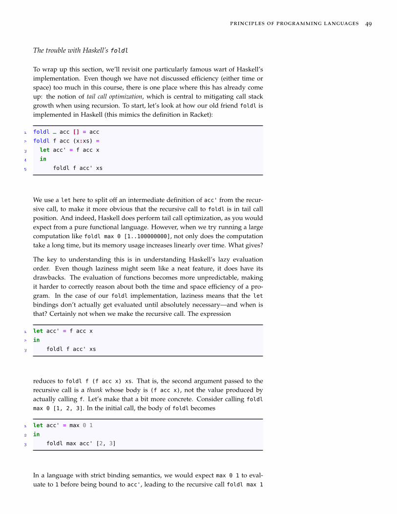
principles of programming languages 49
The trouble with Haskell’s foldl
To wrap up this section, we’ll revisit one particularly famous wart of Haskell’simplementation. Even though we have not discussed efficiency (either time orspace) too much in this course, there is one place where this has already comeup: the notion of tail call optimization, which is central to mitigating call stackgrowth when using recursion. To start, let’s look at how our old friend foldl isimplemented in Haskell (this mimics the definition in Racket):
1 foldl _ acc [] = acc
2 foldl f acc (x:xs) =
3 let acc' = f acc x
4 in
5 foldl f acc' xs
We use a let here to split off an intermediate definition of acc' from the recur-sive call, to make it more obvious that the recursive call to foldl is in tail callposition. And indeed, Haskell does perform tail call optimization, as you wouldexpect from a pure functional language. However, when we try running a largecomputation like foldl max 0 [1..100000000], not only does the computationtake a long time, but its memory usage increases linearly over time. What gives?
The key to understanding this is in understanding Haskell’s lazy evaluationorder. Even though laziness might seem like a neat feature, it does have itsdrawbacks. The evaluation of functions becomes more unpredictable, makingit harder to correctly reason about both the time and space efficiency of a pro-gram. In the case of our foldl implementation, laziness means that the let
bindings don’t actually get evaluated until absolutely necessary—and when isthat? Certainly not when we make the recursive call. The expression
1 let acc' = f acc x
2 in
3 foldl f acc' xs
reduces to foldl f (f acc x) xs. That is, the second argument passed to therecursive call is a thunk whose body is (f acc x), not the value produced byactually calling f. Let’s make that a bit more concrete. Consider calling foldl
max 0 [1, 2, 3]. In the initial call, the body of foldl becomes
1 let acc' = max 0 1
2 in
3 foldl max acc' [2, 3]
In a language with strict binding semantics, we would expect max 0 1 to eval-uate to 1 before being bound to acc', leading to the recursive call foldl max 1

50 david liu
[2, 3]. This is the case in, say, Racket, and combined with tail call optimizationthis leads to space usage that is constant with respect to the size of the inputlist, since the space used to store the accumulator is fixed (a single integer). Inthe case of Haskell, however, acc' is bound to a thunk containing (max 0 1).So then even when the recursive call undergoes tail call optimization, the re-sulting argument data takes a bit more space than before: a thunk instead ofthe initial integer 0. This space usage accumulates35 through the recursive calls,
35 pun definitely intendedwith each new binding of acc' resulting in a new thunk being stored, leadingto the linearly increasing space usage we observe when we call this function.Indeed, these thunks are only called when we reach the end of the list, and acc
is returned and printed (assuming we call this directly in the Haskell REPL).
Because laziness presents its own unique problems, the Haskell language pro-vides ways of explicitly forcing the evaluation of an expression, even when thatexpression’s value is not “necessary” for evaluating its containing outer expres-sion. One approach is with the compiler extension BangPatterns, whose use isillustrated here:
1 {-# LANGUAGE BangPatterns #-}
2
3 foldl _ !acc [] = acc
4 foldl f !acc (x:xs) =
5 let acc' = f acc x
6 in
7 foldl f acc' xs
The only difference, of course, is the first line (telling the compiler to use theBangPatterns extension), and the exclamation mark preceding the acc parame-ter in the function definition. This has the effect of making acc a strict parameter:whenever foldl is called, the argument expression corresponding to acc mustbe evaluated before being passed to foldl, and of course this includes recursivecalls. With this implementation of foldl we get the constant space evaluationof foldl max 0 [1..100000000], taking advantage of both tail call optimizationand eager evaluation of the calls to f to ensure that only an integer accumulatoris passed through the recursive calls.
A final note: why did we call foldl one of Haskell’s “famous warts”? It turnsout that even though this is a well-known issue in the Haskell community, forhistorical reasons the more naturally-named function, foldl, behaves in the lazyway and so is generally discouraged. Instead, users wanting to use the morespace-efficient version can import foldl' from Data.List, paying the price ofboth an extra import and a clumsier name. Go figure.
Lexical closures
To end this chapter, we’ll study in more detail one of the most interesting im-plementation details of a functional programming language: supporting the dy-

principles of programming languages 51
namic creation of functions in a space-efficient manner. Recall the make-adder
function, which takes a number x and returns a new “add x” function:
1 (define (make-adder x)
2 (lambda (y) (+ x y)))
Suppose we call make-adder multiple times: (make-adder 10), (make-adder
-1), (make-adder 9000), etc. A naive (but correct!) implementation of Racketwould create and store in memory brand-new functions for each call:
1 ; (make-adder 10)
2 (lambda (y) (+ x 10))
3 ; (make-adder -1)
4 (lambda (y) (+ x -1))
5 ; (make-adder 9000)
6 (lambda (y) (+ x 9000))
But it seems rather wasteful for Racket to create and store in memory brand-newfunctions each time, when really all of the function values have essentially thesame body, differing only in their value of x.
A better implementation factors out the literal lambda expression (lambda (y)
(+ x y)), which is common to all calls to make-adder, and instead stores simplythe binding for x, which can vary for each function call. And in fact, this isexactly what Racket does! An abstract, but more accurate, representation of theprevious example calls is:36
36 Keep in mind that the (lambda (y)
(+ x y)) is stored once in memory, andmake-adder returns just a reference orpointer to that lambda.
1 ; (make-adder 10)
2 (x: 10) '(lambda (y) (+ x y))
3 ; (make-adder -1)
4 (x: -1) '(lambda (y) (+ x y))
5 ; (make-adder 9000)
6 (x: 9000) '(lambda (y) (+ x y))
The data structure storing the reference to the function code, and the binding forx, is called a closure. All along, when we’ve referred to lambdas as “function val-ues”, each one was actually implemented as a closure! Why has this never comeup before? Closures are conceptually necessary only when the function bodyhas a free identifier, which is an identifier that is not local to the function. Thisshould make intuitive sense: suppose we have a function where every identifierin its body is either a parameter, or bound in a local let expression. Then everytime the function is called, all of the data necessary to evaluate that functioncall is contained in the arguments and the function body—no additional lookupnecessary. In the definition of make-adder, the inner lambda expression has a freeidentifier x, and this is the name whose value will need to be looked up in the
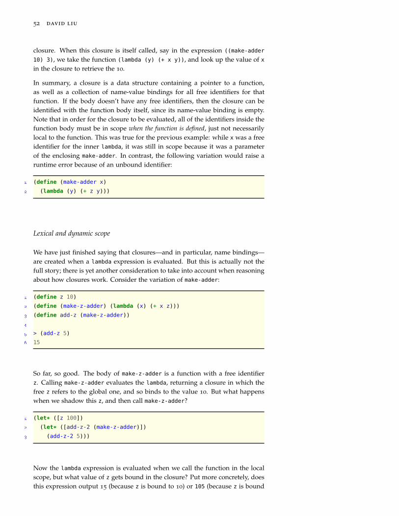
52 david liu
closure. When this closure is itself called, say in the expression ((make-adder
10) 3), we take the function (lambda (y) (+ x y)), and look up the value of xin the closure to retrieve the 10.
In summary, a closure is a data structure containing a pointer to a function,as well as a collection of name-value bindings for all free identifiers for thatfunction. If the body doesn’t have any free identifiers, then the closure can beidentified with the function body itself, since its name-value binding is empty.Note that in order for the closure to be evaluated, all of the identifiers inside thefunction body must be in scope when the function is defined, just not necessarilylocal to the function. This was true for the previous example: while x was a freeidentifier for the inner lambda, it was still in scope because it was a parameterof the enclosing make-adder. In contrast, the following variation would raise aruntime error because of an unbound identifier:
1 (define (make-adder x)
2 (lambda (y) (+ z y)))
Lexical and dynamic scope
We have just finished saying that closures—and in particular, name bindings—are created when a lambda expression is evaluated. But this is actually not thefull story; there is yet another consideration to take into account when reasoningabout how closures work. Consider the variation of make-adder:
1 (define z 10)
2 (define (make-z-adder) (lambda (x) (+ x z)))
3 (define add-z (make-z-adder))
4
5 > (add-z 5)
6 15
So far, so good. The body of make-z-adder is a function with a free identifierz. Calling make-z-adder evaluates the lambda, returning a closure in which thefree z refers to the global one, and so binds to the value 10. But what happenswhen we shadow this z, and then call make-z-adder?
1 (let* ([z 100])
2 (let* ([add-z-2 (make-z-adder)])
3 (add-z-2 5)))
Now the lambda expression is evaluated when we call the function in the localscope, but what value of z gets bound in the closure? Put more concretely, doesthis expression output 15 (because z is bound to 10) or 105 (because z is bound
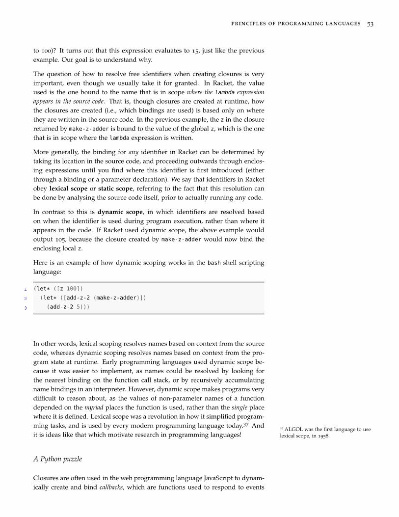
principles of programming languages 53
to 100)? It turns out that this expression evaluates to 15, just like the previousexample. Our goal is to understand why.
The question of how to resolve free identifiers when creating closures is veryimportant, even though we usually take it for granted. In Racket, the valueused is the one bound to the name that is in scope where the lambda expressionappears in the source code. That is, though closures are created at runtime, howthe closures are created (i.e., which bindings are used) is based only on wherethey are written in the source code. In the previous example, the z in the closurereturned by make-z-adder is bound to the value of the global z, which is the onethat is in scope where the lambda expression is written.
More generally, the binding for any identifier in Racket can be determined bytaking its location in the source code, and proceeding outwards through enclos-ing expressions until you find where this identifier is first introduced (eitherthrough a binding or a parameter declaration). We say that identifiers in Racketobey lexical scope or static scope, referring to the fact that this resolution canbe done by analysing the source code itself, prior to actually running any code.
In contrast to this is dynamic scope, in which identifiers are resolved basedon when the identifier is used during program execution, rather than where itappears in the code. If Racket used dynamic scope, the above example wouldoutput 105, because the closure created by make-z-adder would now bind theenclosing local z.
Here is an example of how dynamic scoping works in the bash shell scriptinglanguage:
1 (let* ([z 100])
2 (let* ([add-z-2 (make-z-adder)])
3 (add-z-2 5)))
In other words, lexical scoping resolves names based on context from the sourcecode, whereas dynamic scoping resolves names based on context from the pro-gram state at runtime. Early programming languages used dynamic scope be-cause it was easier to implement, as names could be resolved by looking forthe nearest binding on the function call stack, or by recursively accumulatingname bindings in an interpreter. However, dynamic scope makes programs verydifficult to reason about, as the values of non-parameter names of a functiondepended on the myriad places the function is used, rather than the single placewhere it is defined. Lexical scope was a revolution in how it simplified program-ming tasks, and is used by every modern programming language today.37 And
37 ALGOL was the first language to uselexical scope, in 1958.it is ideas like that which motivate research in programming languages!
A Python puzzle
Closures are often used in the web programming language JavaScript to dynam-ically create and bind callbacks, which are functions used to respond to events

54 david liu
like a user clicking a button or entering some text. A common beginner mistakewhen creating these functions exposes a very subtle misconception about clo-sures when they are combined with mutation. We’ll take a look at an analogousexample in Python.
1 def make_functions():
2 flist = []
3 for i in [1, 2, 3]:
4 def print_i():
5 print(i)
6 print_i()
7 flist.append(print_i)
8 print('End of flist')
9 return flist
10
11 def main():
12 flist = make_functions()
13 for f in flist:
14 f()
15
16 >>> main()
17 1
18 2
19 3
20 End of flist
21 3
22 3
23 3
The fact that Python also uses lexical scope means that the closure of each of thethree print_i functions refers to the same i variable (in the enclosing scope).That is, the closures here store a reference, and not a value.38 After the loop exits,
38 Since we have been avoiding mutationup to this point, there hasn’t yet been adistinction between the two.
i has value 3, and so each of the functions prints the value 3. Note that theclosures of the functions store this reference even after make_functions exits,and the local variable i goes out of scope!
By the way, if you wanted to fix this behaviour, one way would be to not use thei variable directly in the created functions, but instead pass its value to anotherhigher-order function. In the code below, each print_i function has a closurelooking up x, which is bound to different values and not changed as the loopiterates.
1 def create_printer(x):
2 def print_x():
3 print(x)
4 return print_x
5
6 def make_functions():

principles of programming languages 55
7 flist = []
8 for i in [1, 2, 3]:
9 print_i = create_printer(i)
10 print_i()
11 flist.append(print_i)
12 print('End of loop')
13
14 def main():
15 flist = make_functions()
16 for f in flist:
17 f()
Secret sharing
Here’s one more cute example of using closures to allow “secret” communicationbetween two functions in Python.39
39 The nonlocal keyword is used toprevent name shadowing, which wouldhappen if a local secret variable werecreated.
1 def make_secret():
2 secret = ''
3
4 def alice(s):
5 nonlocal secret
6 secret = s
7
8 def bob():
9 nonlocal secret
10 print(secret)
11 # Reset secret
12 secret = ''
13
14 return alice, bob
15
16 >>> alice, bob = make_secret()
17 >>> alice('Hi bob!')
18 >>> bob()
19 Hi bob!
20 >>> secret
21 Error ...
Exercise Break!
1.35 In the following lambda expressions, what are the free identifiers (if any)?(Remember that this is important for understanding what a closure actuallystores.)
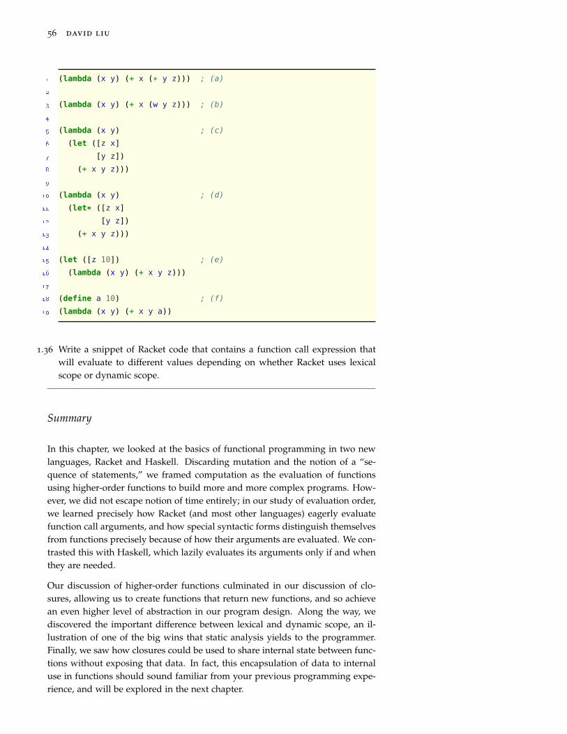
56 david liu
1 (lambda (x y) (+ x (* y z))) ; (a)
2
3 (lambda (x y) (+ x (w y z))) ; (b)
4
5 (lambda (x y) ; (c)
6 (let ([z x]
7 [y z])
8 (+ x y z)))
9
10 (lambda (x y) ; (d)
11 (let* ([z x]
12 [y z])
13 (+ x y z)))
14
15 (let ([z 10]) ; (e)
16 (lambda (x y) (+ x y z)))
17
18 (define a 10) ; (f)
19 (lambda (x y) (+ x y a))
1.36 Write a snippet of Racket code that contains a function call expression thatwill evaluate to different values depending on whether Racket uses lexicalscope or dynamic scope.
Summary
In this chapter, we looked at the basics of functional programming in two newlanguages, Racket and Haskell. Discarding mutation and the notion of a “se-quence of statements,” we framed computation as the evaluation of functionsusing higher-order functions to build more and more complex programs. How-ever, we did not escape notion of time entirely; in our study of evaluation order,we learned precisely how Racket (and most other languages) eagerly evaluatefunction call arguments, and how special syntactic forms distinguish themselvesfrom functions precisely because of how their arguments are evaluated. We con-trasted this with Haskell, which lazily evaluates its arguments only if and whenthey are needed.
Our discussion of higher-order functions culminated in our discussion of clo-sures, allowing us to create functions that return new functions, and so achievean even higher level of abstraction in our program design. Along the way, wediscovered the important difference between lexical and dynamic scope, an il-lustration of one of the big wins that static analysis yields to the programmer.Finally, we saw how closures could be used to share internal state between func-tions without exposing that data. In fact, this encapsulation of data to internaluse in functions should sound familiar from your previous programming expe-rience, and will be explored in the next chapter.

2 Macros, Objects, and Backtracking
In most programming languages,syntax is complex. Macros have totake apart program syntax, analyzeit, and reassemble it. . . A Lispmacro is not handed a string, but apreparsed piece of source code inthe form of a list, because thesource of a Lisp program is not astring; it is a list. And Lispprograms are really good at takingapart lists and putting them backtogether. They do this reliably,every day.
Mark Jason Dominus
Now that we have some experience with functional programming, we will brieflystudy two other programming language paradigms. The first, object-oriented pro-gramming, is likely very familiar to you, while the second, logic programming, islikely not. Because of our limited time in this course, we will not treat eithertopic with as much detail each deserves, as neither is a true focus of this course.Instead, we will stay in Racket, and implement support for these paradigms intothe Racket programming language itself, and so achieve two goals at once: first,you will gain deeper understanding of these paradigms by studying the de-sign decisions and trade-offs made in implementing them; and second, you willlearn how to use a powerful macro system to fundamentally extend the syntaxand semantics of a programming language itself.

58 david liu
Object-oriented programming: a re-introduction
OOP to me means only messaging,local retention and protection andhiding of state-process, andextreme late-binding of all things.
Alan Kay
Because we have often highlighted the stark differences between imperative andfunctional programming, you may be surprised to learn that our study of func-tions has given us all the tools we need to implement a basic object-orientedsystem like the one you’re familiar with from Python (and other imperative lan-guages).
Recall the definition of a closure: a data structure containing a reference to func-tion code together with the lexical environment storing the values of the freevariables in the function body. Now consider what we mean by an object in atraditional OOP setting: an object is a data structure that stores values called the(instance) attributes of the object, that is also associated with functions called(instance) methods that operate of this data.
This paradigm was developed as a way to organize data that promotes encapsu-lation, separating private concerns of how this data is organized from the publicinterface that determine how other code may interact with the data. Unlike thepure functions we have studied so far, a method always takes a special argu-ment,1 an associated object that we say is calling the method. Though internal
1 This “calling object” is often an im-plicit argument with a fixed keywordname like this or self.
attributes of an object are generally not accessible from outside the object, theyare accessible from within the body of methods that the object calls.
Historically, the centrality of the object itself to call methods and access (pub-lic) attributes led to the natural metaphor of entities sending and respondingto messages for modeling computation. Putting the public/private distinctionfront and centre, we can view an object not as “data + methods”, but rather asan entity that can receive messages from external code, and then respond to thatmessage (say by changing its internal state or returning a value). And of course,“receive a message and return a value” is just another way of describing what afunction does, as we illustrate in the following example:2
2 We’ll use the convention in thesenotes of treating messages to objectsas symbols naming the attribute ormethod to access.
1 (define (point msg)
2 (cond [(equal? msg 'x) 10]
3 [(equal? msg 'y) -5]
4 [else "Unrecognized message"]))
5
6 > (point 'x)
7 10
8 > (point 'y)
9 -5

principles of programming languages 59
Classes as higher-order functions
Of course, this “point object” is not very compelling: it only has attributes but nomethods, making it more like a C struct, and its attribute values are hard-coded.
One solution to the latter problem is to create a point class, a template thatspecifies both the attributes and methods for a type of object. In class-basedobject-oriented programming, every object is an instance of a class, obtainingtheir attributes and methods from the class definition.3 Objects are created by
3 Even though class-based OOP is themost common approach, it is not theonly one. JavaScript uses prototypalinheritance to enable behaviour reuse;objects are not instances of classes, butinstead inherit attributes and methodsdirectly from other objects.
calling a class constructor, a function whose purpose is to return a new instanceof that class, often initializing all of the new instance’s attributes.
To translate this into our language of functions, a constructor for Point is a func-tion that takes two numbers, and returns a function analogous to the one above,except with the 10 and 5 replaced by the constructor’s arguments.4
4 We follow the convention of giving theconstructor the same (capitalized) nameas the class itself.
1 (define (Point x y)
2 (lambda (msg)
3 (cond [(equal? msg 'x) x]
4 [(equal? msg 'y) y]
5 [else "Unrecognized message"])))
6
7 > (define p (Point 2 -100))
8 > (p 'x)
9 2
10 > (p 'y)
11 -100
And now we see explicitly the relationship between closures and objects in thismodel: in the returned function, x and y are free identifiers, and so must havevalues bound in a closure when the Point constructor returns. Moreover, be-cause the identifiers x and y are local to the Point constructor, even though theirvalues are stored in the closure, once the constructor has returned they can’t beaccessed without passing a message to the object.5 This is the property of clo-
5 This is analogous to the secret vari-able in the example at the end of thelast chapter.
sures that enables encapsulation: even though both x and y values are accessibleby passing the right messages to the object, it is certainly possible to implement“private” attributes in this model.
One other point: lexical closures is absolutely required to maintain proper en-capsulation of the attributes. Imagine what would happen if the following codewere executed in a dynamically-scoped language, and what implications thiswould have when we create multiple instances of the same class.
1 (define p (Point 2 3))
2 (let ([x 10])
3 (p 'x))
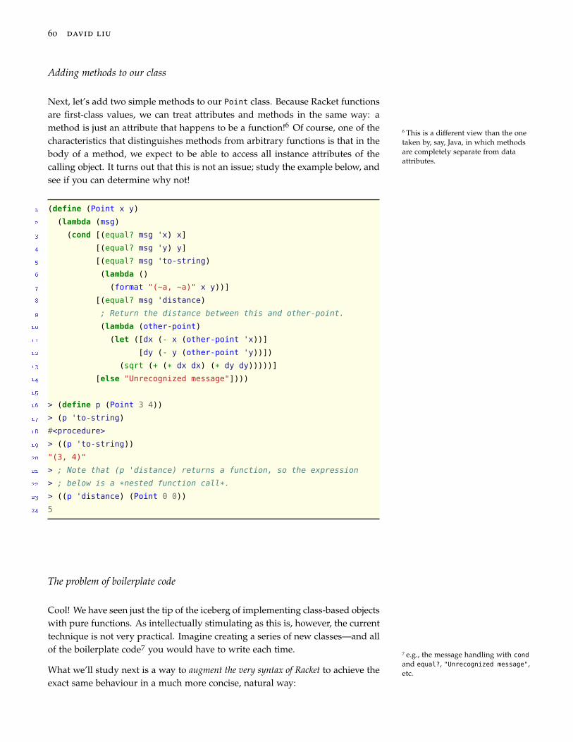
60 david liu
Adding methods to our class
Next, let’s add two simple methods to our Point class. Because Racket functionsare first-class values, we can treat attributes and methods in the same way: amethod is just an attribute that happens to be a function!6 Of course, one of the
6 This is a different view than the onetaken by, say, Java, in which methodsare completely separate from dataattributes.
characteristics that distinguishes methods from arbitrary functions is that in thebody of a method, we expect to be able to access all instance attributes of thecalling object. It turns out that this is not an issue; study the example below, andsee if you can determine why not!
1 (define (Point x y)
2 (lambda (msg)
3 (cond [(equal? msg 'x) x]
4 [(equal? msg 'y) y]
5 [(equal? msg 'to-string)
6 (lambda ()
7 (format "(~a, ~a)" x y))]
8 [(equal? msg 'distance)
9 ; Return the distance between this and other-point.
10 (lambda (other-point)
11 (let ([dx (- x (other-point 'x))]
12 [dy (- y (other-point 'y))])
13 (sqrt (+ (* dx dx) (* dy dy)))))]
14 [else "Unrecognized message"])))
15
16 > (define p (Point 3 4))
17 > (p 'to-string)
18 #<procedure>
19 > ((p 'to-string))
20 "(3, 4)"
21 > ; Note that (p 'distance) returns a function, so the expression
22 > ; below is a *nested function call*.
23 > ((p 'distance) (Point 0 0))
24 5
The problem of boilerplate code
Cool! We have seen just the tip of the iceberg of implementing class-based objectswith pure functions. As intellectually stimulating as this is, however, the currenttechnique is not very practical. Imagine creating a series of new classes—and allof the boilerplate code7 you would have to write each time.
7 e.g., the message handling with cond
and equal?, "Unrecognized message",etc.What we’ll study next is a way to augment the very syntax of Racket to achieve the
exact same behaviour in a much more concise, natural way:
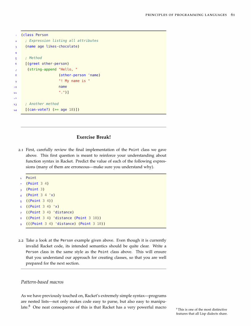
principles of programming languages 61
1 (class Person
2 ; Expression listing all attributes
3 (name age likes-chocolate)
4
5 ; Method
6 [(greet other-person)
7 (string-append "Hello, "
8 (other-person 'name)
9 "! My name is "
10 name
11 ".")]
12
13 ; Another method
14 [(can-vote?) (>= age 18)])
Exercise Break!
2.1 First, carefully review the final implementation of the Point class we gaveabove. This first question is meant to reinforce your understanding aboutfunction syntax in Racket. Predict the value of each of the following expres-sions (many of them are erroneous—make sure you understand why).
1 Point
2 (Point 3 4)
3 (Point 3)
4 (Point 3 4 'x)
5 ((Point 3 4))
6 ((Point 3 4) 'x)
7 ((Point 3 4) 'distance)
8 ((Point 3 4) 'distance (Point 3 10))
9 (((Point 3 4) 'distance) (Point 3 10))
2.2 Take a look at the Person example given above. Even though it is currentlyinvalid Racket code, its intended semantics should be quite clear. Write aPerson class in the same style as the Point class above. This will ensurethat you understand our approach for creating classes, so that you are wellprepared for the next section.
Pattern-based macros
As we have previously touched on, Racket’s extremely simple syntax—programsare nested lists—not only makes code easy to parse, but also easy to manipu-late.8 One neat consequence of this is that Racket has a very powerful macro
8 This is one of the most distinctivefeatures that all Lisp dialects share.
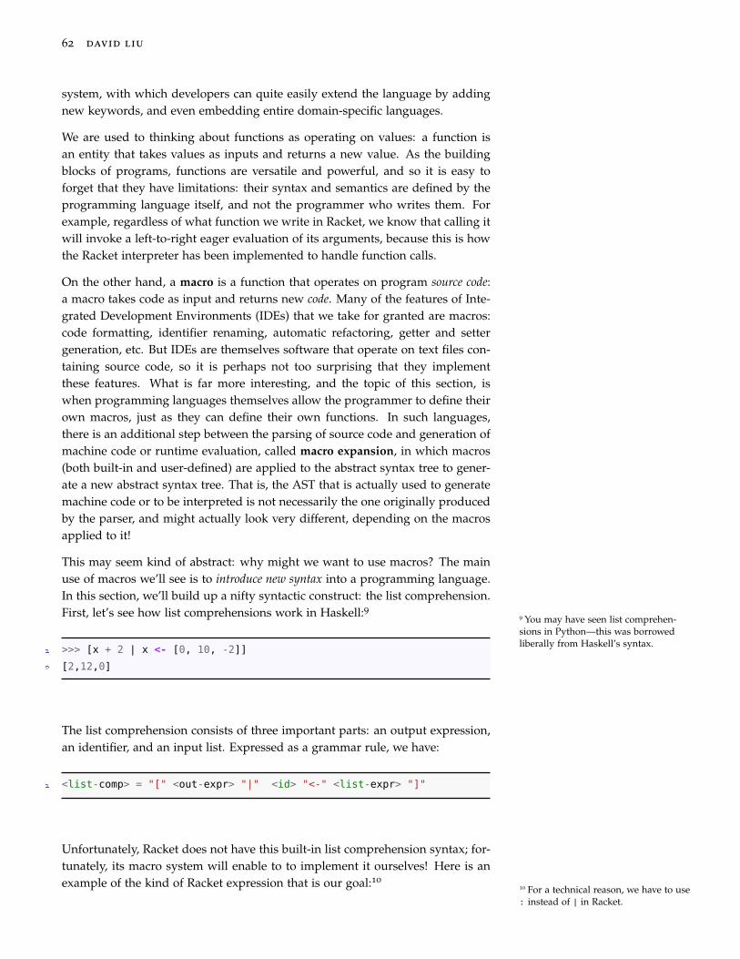
62 david liu
system, with which developers can quite easily extend the language by addingnew keywords, and even embedding entire domain-specific languages.
We are used to thinking about functions as operating on values: a function isan entity that takes values as inputs and returns a new value. As the buildingblocks of programs, functions are versatile and powerful, and so it is easy toforget that they have limitations: their syntax and semantics are defined by theprogramming language itself, and not the programmer who writes them. Forexample, regardless of what function we write in Racket, we know that calling itwill invoke a left-to-right eager evaluation of its arguments, because this is howthe Racket interpreter has been implemented to handle function calls.
On the other hand, a macro is a function that operates on program source code:a macro takes code as input and returns new code. Many of the features of Inte-grated Development Environments (IDEs) that we take for granted are macros:code formatting, identifier renaming, automatic refactoring, getter and settergeneration, etc. But IDEs are themselves software that operate on text files con-taining source code, so it is perhaps not too surprising that they implementthese features. What is far more interesting, and the topic of this section, iswhen programming languages themselves allow the programmer to define theirown macros, just as they can define their own functions. In such languages,there is an additional step between the parsing of source code and generation ofmachine code or runtime evaluation, called macro expansion, in which macros(both built-in and user-defined) are applied to the abstract syntax tree to gener-ate a new abstract syntax tree. That is, the AST that is actually used to generatemachine code or to be interpreted is not necessarily the one originally producedby the parser, and might actually look very different, depending on the macrosapplied to it!
This may seem kind of abstract: why might we want to use macros? The mainuse of macros we’ll see is to introduce new syntax into a programming language.In this section, we’ll build up a nifty syntactic construct: the list comprehension.First, let’s see how list comprehensions work in Haskell:9
9 You may have seen list comprehen-sions in Python—this was borrowedliberally from Haskell’s syntax.
1 >>> [x + 2 | x <- [0, 10, -2]]
2 [2,12,0]
The list comprehension consists of three important parts: an output expression,an identifier, and an input list. Expressed as a grammar rule, we have:
1 <list-comp> = "[" <out-expr> "|" <id> "<-" <list-expr> "]"
Unfortunately, Racket does not have this built-in list comprehension syntax; for-tunately, its macro system will enable to to implement it ourselves! Here is anexample of the kind of Racket expression that is our goal:10
10 For a technical reason, we have to use: instead of | in Racket.
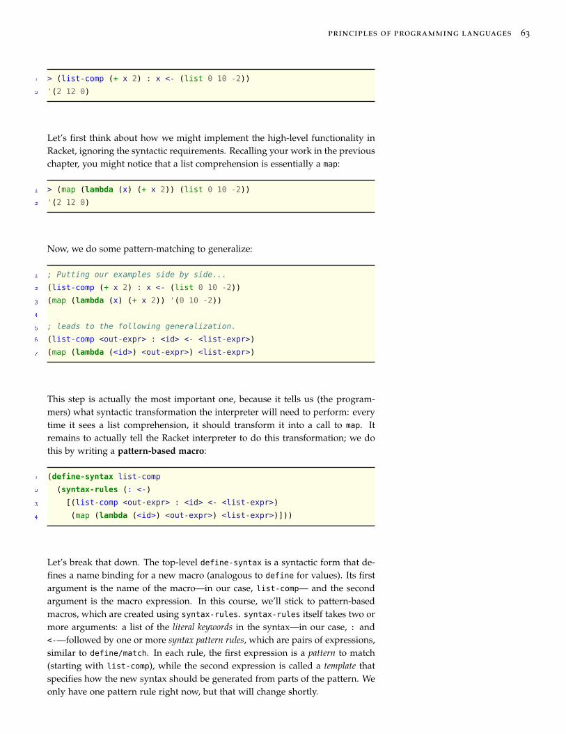
principles of programming languages 63
1 > (list-comp (+ x 2) : x <- (list 0 10 -2))
2 '(2 12 0)
Let’s first think about how we might implement the high-level functionality inRacket, ignoring the syntactic requirements. Recalling your work in the previouschapter, you might notice that a list comprehension is essentially a map:
1 > (map (lambda (x) (+ x 2)) (list 0 10 -2))
2 '(2 12 0)
Now, we do some pattern-matching to generalize:
1 ; Putting our examples side by side...
2 (list-comp (+ x 2) : x <- (list 0 10 -2))
3 (map (lambda (x) (+ x 2)) '(0 10 -2))
4
5 ; leads to the following generalization.
6 (list-comp <out-expr> : <id> <- <list-expr>)
7 (map (lambda (<id>) <out-expr>) <list-expr>)
This step is actually the most important one, because it tells us (the program-mers) what syntactic transformation the interpreter will need to perform: everytime it sees a list comprehension, it should transform it into a call to map. Itremains to actually tell the Racket interpreter to do this transformation; we dothis by writing a pattern-based macro:
1 (define-syntax list-comp
2 (syntax-rules (: <-)
3 [(list-comp <out-expr> : <id> <- <list-expr>)
4 (map (lambda (<id>) <out-expr>) <list-expr>)]))
Let’s break that down. The top-level define-syntax is a syntactic form that de-fines a name binding for a new macro (analogous to define for values). Its firstargument is the name of the macro—in our case, list-comp— and the secondargument is the macro expression. In this course, we’ll stick to pattern-basedmacros, which are created using syntax-rules. syntax-rules itself takes two ormore arguments: a list of the literal keywords in the syntax—in our case, : and<-—followed by one or more syntax pattern rules, which are pairs of expressions,similar to define/match. In each rule, the first expression is a pattern to match(starting with list-comp), while the second expression is called a template thatspecifies how the new syntax should be generated from parts of the pattern. Weonly have one pattern rule right now, but that will change shortly.

64 david liu
With this macro defined, we can now evaluate our Racket list-comp expression:
1 > (list-comp (+ x 2) : x <- (list 0 10 -2))
2 '(2 12 0)
While this might look just like a plain function call, it isn’t! There are two phasesinvolved to produce the result '(2 12 0):
1. First, the list-comp expression is transformed into a map function call expres-sion, by applying the syntax pattern rule we defined. This is a code transfor-mation; you could achieve the same effect by literally typing in (map (lambda
(x) (+ x 2)) (list 0 10 -2)) instead.2. Second, the map expression is evaluated, using plain old function call seman-
tics.
One way to see the difference between list-comp and a regular function is touse the syntax in incorrect ways:
1 > (list-comp 1 2 3)
2 list-comp: bad syntax in: (list-comp 1 2 3)
3 > (list-comp (+ x 2) : x <- 10)
4 map: contract violation
5 expected: list?
6 given: 10
7 argument position: 2nd
8 other arguments...:
9 #<procedure>
The first error is a syntax error: Racket is saying that it doesn’t have a syntaxpattern rule that matches the given expression. The second error really demon-strates that a syntax transformation occurs: (list-comp (+ x 2) : x <- 10)}
might be syntactically valid, but it expands into (map (lambda (x) (+ x 2))
10), which raises the runtime error you see above.
The purpose of literal keywords
Our syntax pattern rule makes use of both pattern variables and literal key-words. A pattern variable is an identifier that can be bound to an arbitraryexpression when the pattern matches; in this course, we’ll follow a conven-tion of naming these with enclosing angle brackets, but this is not required byRacket. During macro expansion, when Racket finds a pattern-match, it bindsthe pattern variable to the corresponding expression, and then substitutes thisexpression where ever the variable appears in the rule’s template. This is sim-ilar to function calls, in which argument values are bound to parameter names
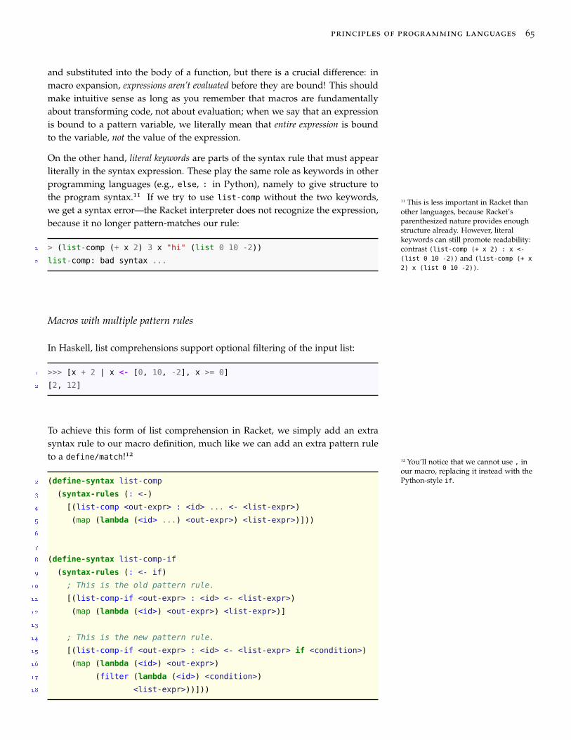
principles of programming languages 65
and substituted into the body of a function, but there is a crucial difference: inmacro expansion, expressions aren’t evaluated before they are bound! This shouldmake intuitive sense as long as you remember that macros are fundamentallyabout transforming code, not about evaluation; when we say that an expressionis bound to a pattern variable, we literally mean that entire expression is boundto the variable, not the value of the expression.
On the other hand, literal keywords are parts of the syntax rule that must appearliterally in the syntax expression. These play the same role as keywords in otherprogramming languages (e.g., else, : in Python), namely to give structure tothe program syntax.11 If we try to use list-comp without the two keywords,
11 This is less important in Racket thanother languages, because Racket’sparenthesized nature provides enoughstructure already. However, literalkeywords can still promote readability:contrast (list-comp (+ x 2) : x <-
(list 0 10 -2)) and (list-comp (+ x
2) x (list 0 10 -2)).
we get a syntax error—the Racket interpreter does not recognize the expression,because it no longer pattern-matches our rule:
1 > (list-comp (+ x 2) 3 x "hi" (list 0 10 -2))
2 list-comp: bad syntax ...
Macros with multiple pattern rules
In Haskell, list comprehensions support optional filtering of the input list:
1 >>> [x + 2 | x <- [0, 10, -2], x >= 0]
2 [2, 12]
To achieve this form of list comprehension in Racket, we simply add an extrasyntax rule to our macro definition, much like we can add an extra pattern ruleto a define/match!12
12 You’ll notice that we cannot use , inour macro, replacing it instead with thePython-style if.2 (define-syntax list-comp
3 (syntax-rules (: <-)
4 [(list-comp <out-expr> : <id> ... <- <list-expr>)
5 (map (lambda (<id> ...) <out-expr>) <list-expr>)]))
6
7
8 (define-syntax list-comp-if
9 (syntax-rules (: <- if)
10 ; This is the old pattern rule.
11 [(list-comp-if <out-expr> : <id> <- <list-expr>)
12 (map (lambda (<id>) <out-expr>) <list-expr>)]
13
14 ; This is the new pattern rule.
15 [(list-comp-if <out-expr> : <id> <- <list-expr> if <condition>)
16 (map (lambda (<id>) <out-expr>)
17 (filter (lambda (<id>) <condition>)
18 <list-expr>))]))

66 david liu
With these two rules in place, we now can use both our original and extendedform of list-comp:
1 > (list-comp-if (+ x 2) : x <- (list 0 10 -2))
2 '(2 12 0)
3 > (list-comp-if (+ x 2) : x <- (list 0 10 -2) if (>= x 0))
4 '(2 12)
As with functions defined using pattern-matching in both Racket and Haskell,macro pattern rules are checked top-to-bottom, with the first match being theone that is chosen. In this example the rules are mutually exclusive, but ingeneral it’s certainly possible to define two syntax pattern rules that overlap, sobe careful about this when writing your own macros!
Text-based vs. AST-based macros
If you’ve heard of macros before learning a Lisp-family language, it was prob-ably from C or C++.13 The C macro system operates on the source text itself,
13 The typesetting language LaTeX alsouses macros extensively.rather than a parsed AST. In the macro example above we noted that we couldn’t
use | or , as literal keywords; this is because they are special characters that af-fect the parsing of Racket code into an AST, and so have an effect even before themacro expansion phase. This limitation aside, it is far easier and safer to defineAST-based macros. In this section, we look at two examples of how text-basedC macros can lead to unexpected pitfalls.
First, here is a simple example of a C macro that takes one argument and multi-plies its argument by 2:
1 #define double(x) 2 * x
When we use this macro on an integer literal or an identifier, things seem towork fine:
1 #include <stdio.h>
2
3 #define double(x) 2 * x
4
5 int main(void) {
6 int a = 10;
7 printf("%d\n", double(100)); // Correctly prints 200.
8 printf("%d\n", double(a)); // Correctly prints 20.
9 return 0;
10 }

principles of programming languages 67
In each of the above invocations, the source text involving double is replaced:double(100) by 2 * 100 and double(a) by 2 * a. But consider this usage of themacro instead:
1 printf("%d\n", double(5 + 5));
Our intuition tells us that again 20 would be printed, but this is not what hap-pens! To see what goes wrong, we need to understand how the substitutionworks in C macros. Like Racket, macros in C do not evaluate their argumentsbefore substitution; instead, the entire subexpression 5 + 5 is substituted for x
into the body of the macro. The problem arises from the fact that this is a text-based substitution; since the body of the macro is (in text) 2 * x, the resultingmacro expansion yields 2 * 5 + 5, and so 15 is printed!
In other words, because C macros use text-based substitution, their argumentsare not necessarily preserved as individual subexpressions when put into themacro body—it depends on how the compiler then parses the resulting text.In the above example, the precedence rules governing the parsing of arithmeticexpressions caused the 5 + 5 to be split up.
To prevent this, a common rule of thumb when writing C macros is to alwaysparenthesize macro variables in the macro body:14
14 For a similar reason, another rule ofthumb is to surround the entire macrobody in parentheses when it is a singleexpression.
1 #define double(x) 2 * (x)
Because Racket macros operate on abstract syntax trees, this problem is avoidedentirely. When the substitution occurs, the exact expression structure of theRacket program has already been determined, and macro expansion simplyswaps subexpressions matching a pattern rule with the corresponding template.The only new subexpressions that appear in the resulting AST are the ones thatwere explicitly written in the macro definition, and the macro’s arguments.
Now consider the following macro, which uses a temporary variable to swaptwo integers. It seems to work just fine in this small program.
1 #include <stdio.h>
2
3 #define swap(a, b) int temp = a; a = b; b = temp;
4
5 int main(void) {
6 int x = 0, y = 10;
7 swap(x, y)
8 printf("x is now %d, y is now %d\n", x, y);
9 return 0;
10 }

68 david liu
But we run into a problem when trying to compile the following code:
1 #include <stdio.h>
2
3 #define swap(a, b) int temp = a; a = b; b = temp;
4
5 int main(void) {
6 int x = 0, y = 10;
7 swap(x, y)
8 swap(x, y)
9 printf("x is now %d, y is now %d\n", x, y);
10 return 0;
11 }
We get the message error: redefinition of 'temp'; each use of the macrodeclares a local variable temp, which is a compilation error. Now, C allows forlocal scopes to be introduced through curly braces, and so we can solve thisproblem by enclosing the macro body in curly braces:
1 #define swap(a, b) {int temp = a; a = b; b = temp;}
However, another problem emerges: what if one of the variables we wanted toswap was named temp?
1 #include <stdio.h>
2
3 #define swap(a, b) {int temp = a; a = b; b = temp;}
4
5 int main(void) {
6 int x = 0, temp = 10;
7 swap(x, temp)
8 printf("x is now %d, temp is now %d\n", x, temp);
9 return 0;
10 }
This program compiles successfully, but when run it prints:
1 x is now 0, temp is now 10
The variables weren’t swapped! To see why, we again can look at the literal textsubstitution of swap(x, temp):

principles of programming languages 69
1 {int temp = x; x = temp; temp = temp;}
In this case, all references to temp in the macro are for the block-local temp,not the temp that was initialized to 10 at the top of main. So the local temp isinitialized to the current value of x (0), then x is assigned that value (0), andthen temp is assigned its current value. After the block executes, the values of xand temp haven’t changed at all.
A third approach is to require declaration of temp before using this macro. Thisdoes work correctly, at the cost of an additional requirement placed on users ofthis macro.
1 #include <stdio.h>
2
3 #define swap(a, b) {temp = a; a = b; b = temp;}
4
5 int main(void) {
6 int x = 0, y = 10, temp;
7 swap(x, y);
8 printf("x is now %d, y is now %d\n", x, y);
9 return 0;
10 }
These three examples of swap illustrate the ways in which the body of a C macrocan interact with the scope in which it is used: first, introducing names into theouter scope; second, by inadvertently shadowing identifiers that are passed asarguments to the macro; and third, by directly accessing (and mutating) valuesfrom that outer scope. The ability for a C macro to refer to identifiers defined inan outer scope is known as name capture, and is a common source of error whenwriting C macros. The behaviour of these macros depends not just on howthey’re defined, but on where they are used. If this sounds familiar, it should!Identifiers in C macros obey dynamic scope.
That C macros behave in this ways is a natural consequence of how identifiersare just substituted as text during macro expansion. Even though we knowthat Racket macros are based on AST transformation, it is still plausible forindividual identifiers to be substituted as-is during macro expansion. Let’s tryout a simple example and see what happens.
1 (define-syntax add-temp
2 (syntax-rules ()
3 [(add-temp <x>)
4 (+ <x> temp)]))

70 david liu
It may look like temp is undefined in the body of add-temp, much like temp
was undeclared in the macro body of our third example. The question is, whathappens with:
1 (let* ([temp 10])
2 (add-temp 100))
Using a literal textual substitution of identifiers, after macro expansion this ex-pression would become
1 (let* ([temp 10])
2 (+ 100 temp))
This is certainly a valid Racket expression, and would evaluate to 110. However,this is not what happens!
1 > (let* ([temp 10])
2 (add-temp 100))
3 ERROR temp: undefined;
4 cannot reference an identifier before its definition
That is, the temp in the add-temp macro template obeys lexical scope, and cannotbe bound dynamically where the macro is used.
This is true for all Racket macros: free identifiers in the macro obey lexical scope,meaning they are bound to whatever identifier is in scope where the macro isoriginally defined, and cannot accidentally bind names when it is used. Becausethis was seen as a massive improvement over the previous dynamically-scopedmacros, early developers of Lisp termed this form of macro hygienic macros.15
15 This behaviour suggests somethinginteresting about macro expansionin Racket. It isn’t just that expan-sion occurs at the level of ASTs; evenindividual identifiers are just not substi-tuted literally during expansion. Whilethe exact implementation of hygienicmacros are beyond the scope of thiscourse, a simplified mental model youcan use here is that all local identifiersin a macro body are renamed duringexpansion to guarantee that there areno collisions with the scope in whichthe macro is used.
As a consequence of macro hygiene, identifiers defined within a macro body arenot accessible outside of the macro body—that is, they’re local to the macro—even when a straight textual substitution would suggest otherwise. For example:
1 (define-syntax defs
2 (syntax-rules ()
3 [(defs)
4 (begin ; We use begin to enclose multiple expressions
5 (define x 1)
6 (define y (+ x 10))
7 ; x and y are both in scope here.
8 (+ x y))]))
9
10 (defs) ; This evaluates to 12
11 x ; This is an error! x and y are not in scope.

principles of programming languages 71
Contrast this behaviour against simply using the begin instead of our defs
macro:
1 ; This still evaluates to 12
2 (begin
3 (define x 1)
4 (define y (+ x 10))
5 (+ x y))
6
7 ; But now x is defined as well! The following evaluates to 1.
8 x
Macro ellipses
It is often the case that we want a macro that can be applied to an arbitrarynumber of expressions.16 This poses a challenge when writing macro pattern
16 e.g., and, or, condrules, as we can’t write an explicit pattern variable for each expression we expectto match. Instead, we can use the ellipsis ... in a pattern: <pat> ... matcheszero or more instances of the pattern <pat>, which could be a pattern variableor a complex pattern itself.17
17 This is analogous to the * operator inregular expressions, which can matchan arbitrary number of any character(.*) or a complex pattern (a[0-9]*)*.
Here is one example of using the ellipsis in a recursive macro that implementscond in terms of if. Recall that branching of “else if” expressions can be rewrit-ten in terms of nested if expressions:
1 (cond [c1 x1]
2 [c2 x2]
3 [c3 x3]
4 [else y])
5
6 ; as one cond inside an if...
7 (if c1
8 x1
9 (cond [c2 x2]
10 [c3 x3]
11 [else y]))
12
13 ; eventually expanding to...
14 (if c1
15 x1
16 (if c2
17 x2
18 (if c3
19 x3
20 y)))
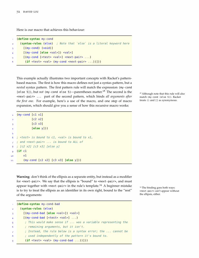
72 david liu
Here is our macro that achieves this behaviour:
1 (define-syntax my-cond
2 (syntax-rules (else) ; Note that `else` is a literal keyword here
3 [(my-cond) (void)]
4 [(my-cond [else <val>]) <val>]
5 [(my-cond [<test> <val>] <next-pair> ...)
6 (if <test> <val> (my-cond <next-pair> ...))]))
This example actually illustrates two important concepts with Racket’s pattern-based macros. The first is how this macro defines not just a syntax pattern, but anested syntax pattern. The first pattern rule will match the expression (my-cond
[else 5]), but not (my-cond else 5)—parentheses matter.18 The second is the18 Although note that this rule will alsomatch (my-cond (else 5)). Rackettreats () and [] as synonymous.
<next-pair> ... part of the second pattern, which binds all arguments afterthe first one. For example, here’s a use of the macro, and one step of macroexpansion, which should give you a sense of how this recursive macro works:
1 (my-cond [c1 x1]
2 [c2 x2]
3 [c3 x3]
4 [else y]))
5
6 ; <test> is bound to c1, <val> is bound to x1,
7 ; and <next-pair> ... is bound to ALL of
8 ; [c2 x2] [c3 x3] [else y]
9 (if c1
10 x1
11 (my-cond [c2 x2] [c3 x3] [else y]))
Warning: don’t think of the ellipsis as a separate entity, but instead as a modifierfor <next-pair>. We say that the ellipsis is “bound” to <next-pair>, and mustappear together with <next-pair> in the rule’s template.19 A beginner mistake
19 The binding goes both ways:<next-pair> can’t appear withoutthe ellipsis, either.
is to try to treat the ellipsis as an identifier in its own right, bound to the “rest”of the arguments:
1 (define-syntax my-cond-bad
2 (syntax-rules (else)
3 [(my-cond-bad [else <val>]) <val>]
4 [(my-cond-bad [<test> <val>] ...)
5 ; This would make sense if ... was a variable representing the
6 ; remaining arguments, but it isn't.
7 ; Instead, the rule below is a syntax error; the ... cannot be
8 ; used independently of the pattern it's bound to.
9 (if <test> <val> (my-cond-bad ...))]))

principles of programming languages 73
To summarize, a pattern variable that is modified with an ellipsis is no longerbound to an individual expression, but instead to the entire sequence of expres-sions. We’ll see how to make powerful use of this sequence in the next section.
Exercise Break!
2.3 Explain how a macro is different from a function. Explain how it is similar toa function.
2.4 Below, we define a macro, and then use it in a few expressions. Write theresulting expressions after the macros are expanded. Note: do not evaluateany of the resulting expressions! This question is a good check to make sureyou understand the difference between the macro expansion and evaluationphases of the Racket interpreter.
1 (define-syntax my-mac
2 (syntax-rules ()
3 [(my-mac x) (list x x)]))
4
5 (my-mac 3)
6 (my-mac (+ 4 2))
7 (my-mac (my-mac 1000))
2.5 Write macros to implement and and or in terms of if. Note that both syntacticforms take an arbitrary number of arguments.
2.6 Why could we not accomplish the task in the previous question with func-tions?
2.7 Consult the official Haskell documentation on list comprehensions. One ad-ditional feature we did not cover is list comprehensions on multiple variables.
Modify our existing list-comp macro to handle this case. Hint: first convertthe above expression into a list comprehension within a list comprehension,and use apply append.
2.8 Add support for ifs in list comprehensions with multiple variables. Are thereany syntactic issues you need to think through?
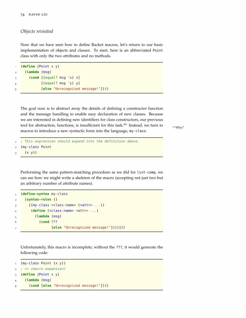
74 david liu
Objects revisited
Now that we have seen how to define Racket macros, let’s return to our basicimplementation of objects and classes. To start, here is an abbreviated Point
class with only the two attributes and no methods.
1 (define (Point x y)
2 (lambda (msg)
3 (cond [(equal? msg 'x) x]
4 [(equal? msg 'y) y]
5 [else "Unrecognized message!"])))
The goal now is to abstract away the details of defining a constructor functionand the message handling to enable easy declaration of new classes. Becausewe are interested in defining new identifiers for class constructors, our previoustool for abstraction, functions, is insufficient for this task.20 Instead, we turn to
20 Why?macros to introduce a new syntactic form into the language, my-class:
1 ; This expression should expand into the definition above.
2 (my-class Point
3 (x y))
Performing the same pattern-matching procedure as we did for list-comp, wecan see how we might write a skeleton of the macro (accepting not just two butan arbitrary number of attribute names).
1 (define-syntax my-class
2 (syntax-rules ()
3 [(my-class <class-name> (<attr> ...))
4 (define (<class-name> <attr> ...)
5 (lambda (msg)
6 (cond ???
7 [else "Unrecognized message!"])))]))
Unfortunately, this macro is incomplete; without the ???, it would generate thefollowing code:
1 (my-class Point (x y))
2 ; => (macro expansion)
3 (define (Point x y)
4 (lambda (msg)
5 (cond [else "Unrecognized message!"])))

principles of programming languages 75
What’s missing, of course, are the other expressions in the cond that match mes-sages corresponding to the attribute names. Let’s consider the first attribute x.For this attribute, we want to generate the code
1 [(equal? msg 'x) x]
Now, to do this we need some way of converting an identifier into a symbol,which we can do using the syntactic form quote:
1 [(equal? msg (quote x) x)]
For (my-class Point (x y)), we actually want this expression to appear forboth x and y:
1 [(equal? msg (quote x) x)]
2 [(equal? msg (quote y) y)]
So the question is how to generate one of these expressions for each of the at-tributes bound to <attr> ...; that is, repeat the above pattern an arbitrary num-ber of times, depending on the number of attributes. It turns out that macroellipses support precisely this behaviour:21
21 I hope you’re suitably impressed. Iknow I am.
1 (define-syntax my-class
2 (syntax-rules ()
3 [(my-class <class-name> (<attr> ...))
4 (define (<class-name> <attr> ...)
5 (lambda (msg)
6 (cond [(equal? msg (quote <attr>)) <attr>]
7 ; Repeat the previous expression once per expression
8 ; in <attr> ..., replacing just occurrences of <attr>
9 ...
10 [else "Unrecognized message!"])))]))
Adding methods
Now, let us augment our macro to allow method definitions. Even though wepreviously made a stink about methods just being any other type of attribute,there is one important difference: it isn’t enough to provide just the name of themethod in the class definition; we need to provide the method body as well. Wewill use the following syntax, mimicking Racket’s own macro pattern-matchingsyntax:

76 david liu
1 (my-class <class-name> (<attr> ...)
2 (method (<method-name> <param> ...) <body>) ...)
Once again, the easiest way to write the pattern-based macro is to create aninstance of both the syntactic form we want to write, and the expression wewant to expand it into. To use our ongoing point example:
1 ; What we want to write:
2 (my-class Point (x y)
3 (method (distance other-point)
4 (let* ([dx (- x (other-point 'x))]
5 [dy (- y (other-point 'y))])
6 (sqrt (+ (* dx dx) (* dy dy))))))
7
8 ; What we want it to expand into:
9 (define (Point x y)
10 (lambda (msg)
11 (cond [(equal? msg 'x) x]
12 [(equal? msg 'y) y]
13 [(equal? msg 'distance)
14 (lambda (other-point)
15 (let* ([dx (- x (other-point 'x))]
16 [dy (- y (other-point 'y))])
17 (sqrt (+ (* dx dx) (* dy dy)))))])))
After carefully examining these two expressions, the pieces just fall into place:22
22 This showcases the use of nestedellipses in a pattern expression. Holycow, that rocks! Racket’s insistence inalways pairing an ellipsis with a namedidentifier and strict use of parenthesesreally help distinguish the ellipsispairings.
1 (define-syntax my-class
2 (syntax-rules (method)
3 [(my-class <class-name>
4 ; This ellipsis is paired with <attr>
5 (<attr> ...)
6 ; This ellipsis is paired with <param>
7 (method (<method-name> <param> ...) <body>)
8 ; This ellipsis is paired with the whole previous pattern
9 ...)
10 (define (<class-name> <attr> ...)
11 (lambda (msg)
12 (cond [(equal? msg (quote <attr>)) <attr>]
13 ...
14 [(equal? msg (quote <method-name>))
15 (lambda (<param> ...) <body>)]
16 ...
17 [else "Unrecognized message!"])))]))

principles of programming languages 77
The object __dict__
You might notice that the repeated (equal? msg <symbol>) clauses of the cond
implement a (slow!) dictionary lookup, where the name of an attribute is keyedto its value for that object. Indeed, in Python every object has a special attribute__dict__ that refers precisely to its dictionary of attributes (but not methods—more on this later):
1 class A:
2 def __init__(self, x):
3 self.x = x
4 self.y = 10
5 self.z = 'hello!'
6
7 >>> a = A(True)
8 >>> a.__dict__
9 {'x': True, 'y': 10, 'z': 'hello!'}
We can improve the performance of our my-class macro by using a built-inhashing data structure in Racket to store our attributes and methods.
3 (define-syntax my-class
4 (syntax-rules (method)
5 [(my-class <class-name> (<attr> ...)
6 (method (<method-name> <param> ...) <body>) ...)
7
8 (define (<class-name> <attr> ...)
9 (lambda (msg)
10 (let* ([__dict__ ; Use the same name as Python
11 (make-immutable-hash
12 (list (cons (quote <attr>) <attr>)
13 ...
14 (cons (quote <method-name>)
15 (lambda (<param> ...) <body>))
16 ...
17 ))])
18
19 ; Look up the given attribute in the object's dictionary.
20 (hash-ref __dict__ msg
21 ; Raise an error if attribute not found.
22 (attribute-error (quote <class-name>) msg)))))]))
23
24 ; Return a thunk that raises an attribute error (with an appropriate message).
25 (define (attribute-error object attr)
26 (lambda () (error (format "~a has no attribute ~a." object attr))))

78 david liu
Exercise Break!
2.9 Modify the __dict__-based class implementation to enable accessing the __dict__
value from outside the object, as we can in Python. For example:
1 > (define p (Point 2 3))
2 > (p '__dict__)
3 '#hash((x . 2) (y . 3))
Note that in Python, the __dict__ attribute itself doesn’t appear in the object’sdictionary. Can you achieve the same effect in Racket?
The problem of self
So far, our implementation of classes may seem to work, but it has one major de-ficiency: we cannot explicitly reference the calling object in a method. Considerthe following example in Python:
1 class Point:
2 def __init__(self, x, y):
3 self.x = x
4 self.y = y
5
6 def size(self):
7 return math.sqrt(self.x ** 2 + self.y ** 2)
8
9 def same_radius(self, other):
10 return self.size() == other.size()
Our current implementation has no trouble implementing the initializer method__init__ (it does this automatically), and it can handle simple attribute accessof x and y because those identifiers would be bound in the closure returned byour class constructor. However, self.same_radius() poses a problem:
1 (my-class Point (x y)
2 (method (size) (sqrt (+ (* x x) (* y y))))
3 (method (same-radius other)
4 (equal? ??? ((other 'size)))))

principles of programming languages 79
Unlike x and y, there is no size identifier in scope in the closure: instead, 'size isa key in the dictionary, but we have no way to automatically convert it! Perhapsthe most direct way of solving this problem is to modify our macro to introduceidentifiers for each method as well, making them exactly parallel to the “data”attributes that are the constructor parameters:23
23 This models the notion of an implicitthis in, e.g., Java.
1 (method (same-radius other)
2 (equal? (size) (other 'size)))
However, this has the drawback that we still wouldn’t have a way of referencingself, e.g., to pass the calling object to a completely different function. So instead,we’ll look at an approach to make self an accessible identifier, referencing thecalling object:
1 (method (same-radius other)
2 (equal? ((self 'size)) ((other 'size))))
Pythonic inspiration
To guide our design and implementation, let’s first review how self works inPython. You are already familiar with the most visible part: self is an explicitparameter written in every instance method of the class!24 In fact, if we adopt
24 In fact, the name self is just a con-vention: technically, Python interpretsthe first parameter as the one that isbound to the calling object, whateverthe parameter name actually is.
this convention then we can write the following Racket code without makingany changes to our macro at all:
1 (my-class Point (x y)
2 (method (size self) (sqrt (+ (* (self 'x) (self 'x))
3 (* (self 'y) (self 'y)))))
4 (method (same-radius self other)
5 (equal? ((self 'size) self) ((other 'size) other))))
Look at that last line carefully—what’s going on there? Our goal is for (self
'size) to return a function that takes no arguments, so that we can just call it (byenclosing it in parentheses). However, what we have here is that (self 'size)
returns a function that takes a single argument, self, and so we need to passthat argument. The same is true when we call (other 'size), too. Of course,this is very redundant: since we’re calling (self 'size) already, we know whatthe calling object is, and shouldn’t need to pass it in again!
This is solved in Python: an instance method call self.size() automaticallybinds the value to the left of the period, self, to the first parameter of thesize method; the arguments in the parentheses get bound to the remaining
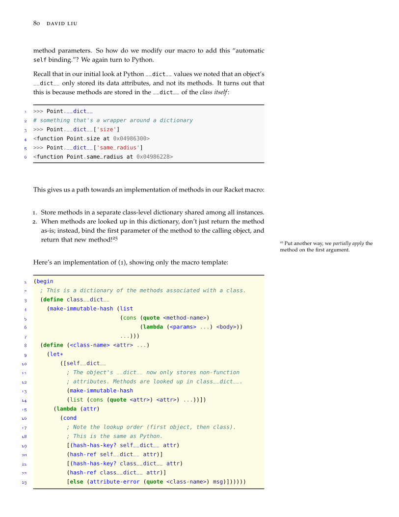
80 david liu
method parameters. So how do we modify our macro to add this “automaticself binding.”? We again turn to Python.
Recall that in our initial look at Python __dict__ values we noted that an object’s__dict__ only stored its data attributes, and not its methods. It turns out thatthis is because methods are stored in the __dict__ of the class itself :
1 >>> Point.__dict__
2 # something that's a wrapper around a dictionary
3 >>> Point.__dict__['size']
4 <function Point.size at 0x04986300>
5 >>> Point.__dict__['same_radius']
6 <function Point.same_radius at 0x04986228>
This gives us a path towards an implementation of methods in our Racket macro:
1. Store methods in a separate class-level dictionary shared among all instances.2. When methods are looked up in this dictionary, don’t just return the method
as-is; instead, bind the first parameter of the method to the calling object, andreturn that new method!25
25 Put another way, we partially apply themethod on the first argument.
Here’s an implementation of (1), showing only the macro template:
1 (begin
2 ; This is a dictionary of the methods associated with a class.
3 (define class__dict__
4 (make-immutable-hash (list
5 (cons (quote <method-name>)
6 (lambda (<params> ...) <body>))
7 ...)))
8 (define (<class-name> <attr> ...)
9 (let*10 ([self__dict__
11 ; The object's __dict__ now only stores non-function
12 ; attributes. Methods are looked up in class__dict__.
13 (make-immutable-hash
14 (list (cons (quote <attr>) <attr>) ...))])
15 (lambda (attr)
16 (cond
17 ; Note the lookup order (first object, then class).
18 ; This is the same as Python.
19 [(hash-has-key? self__dict__ attr)
20 (hash-ref self__dict__ attr)]
21 [(hash-has-key? class__dict__ attr)
22 (hash-ref class__dict__ attr)]
23 [else (attribute-error (quote <class-name>) msg)])))))

principles of programming languages 81
This is a little longer, but conceptually the only thing we’ve done is taken ouroriginal object dictionary and split it in to two, putting the data attributes in oneand the methods in the other. (Unfortunately, our methods can’t access instancevariables anymore, because methods are no longer in the lambda (<params>
...) closure. We’ll fix that in our next iteration.)
However, this alone doesn’t solve (2). First, we introduce the function fix-first,26
26 We leave the implementation of thisfunction as an exercise.which is a higher-order function that takes a function f that takes n + 1 argu-
ments, and a value x, and returns a function g that takes n arguments, such thatg(x1, x2, ..., xn) is equivalent to f(x, x1, x2, ... xn). So then in the sec-ond branch of the cond, we can do (fix-first ??? (hash-ref class_dict__
attr)). But what goes in the ???? We need a way to refer to the object itself—and remember that the “object” is the entire lambda expression itself. In otherwords, this expression needs to be recursive; we can do this by using letrec:
6 (define-syntax my-class
7 (syntax-rules (method)
8 [(my-class <class-name> (<attr> ...)
9 (method (<method-name> <params> ...) <body>) ...)
10
11 (begin
12 ; This is a dictionary of the methods associated with a class.
13 (define class__dict__
14 (make-immutable-hash (list
15 (cons (quote <method-name>)
16 (lambda (<params> ...) <body>))
17 ...)))
18 (define (<class-name> <attr> ...)
19 ; We use letrec to give a name to the object we're returning.
20 ; This is so that we can bind the object to the 'self'
21 ; parameter in the call to fix-first.
22 (letrec
23 ([self__dict__
24 ; The object's __dict__ now only stores non-function
25 ; attributes. Methods are looked up in class__dict__.
26 (make-immutable-hash
27 (list (cons (quote <attr>) <attr>) ...))]
28 [me (lambda (attr)
29 (cond
30 [(hash-has-key? self__dict__ attr)
31 (hash-ref self__dict__ attr)]
32 [(hash-has-key? class__dict__ attr)
33 (fix-first me (hash-ref class__dict__ attr))]
34 [else
35 ((attribute-error (quote <class-name>) attr))]))])
36 ; Return the lambda representing the object.
37 me)))]))

82 david liu
The power of chained lookups
In the previous section, we used the idea of a lookup chain to separate instanceattributes and methods. The idea of using multiple dictionaries to store dif-ferent kinds of “attributes” is a versatile technique, and is commonly used ininterpreters to implement different forms of inheritance. In Python, for exam-ple, since each class has its own __dict__, it is straightforward to implementmethod inheritance simply by inspecting the sequence of superclasses until themethod is found.27
27 This works even though Pythonsupports multiple inheritance; the built-in mro function, standing for methodresolution order, returns a sequence ofthe superclasses in the order they arechecked for a given method.
JavaScript dispenses with the notion of separate “classes”, and instead supportsa chain of objects directly. In this language, almost every object keeps a referenceto another object, called its prototype. When an attribute is accessed on an object,the object’s own “dictionary” is checked first; if the attribute isn’t found, theobject’s prototype is checked, and then the object’s prototype’s prototype, andso on until the root “base object” (with no prototype) is reached. This formof inheritance is known as prototypal inheritance, distinguishing it from the class-based inheritance of Python and other languages. But fundamentally, both class-based and prototypal inheritance can be thought of as variations of the same ideaof chained lookups!
Exercise Break!
Each of these exercises involves extending our basic class macro in interestingways. Be warned that these are more challenging than the usual exercises.
2.10 Modify the my-class macro to add support for private attributes.
2.11 Modify the my-class macro to add support for some form of inheritance, asdescribed in the previous section.

principles of programming languages 83
Manipulating control flow I: streams
In the first half of this chapter, we saw how to use macros to introduce newsyntactic forms to reduce boilerplate code and create name bindings for classes.Hopefully this gave you a taste of the flexibility and power of macros: by chang-ing the very syntax of our core language, we enable new paradigms, and hencenew idioms and techniques for crafting software. Now, we’ll start to look moreexplicitly at another common usage of macros: manipulating control flow tocircumvent the eager evaluation of function calls in Racket.
Our first foray into this area will be to implement streams, a “lazy” analogue ofthe familiar list data type. First, recall the recursive definition of a list:
• A list is either empty, or• A value “cons’d” with another list.
In Racket, cons is a function, and so all lists built up using cons are eagerly eval-uated: all list elements are evaluated when the list is constructed.28 However,
28 The same is true of the Racket built-inlist, as it too is a function.this is often not necessary: when we traverse a list, we often only care about
accessing one element at a time, and do not need the other elements to havebeen evaluated at this point. This motivates our implementation of a stream inRacket, which follows the following recursive definition:
• A stream is either empty, or• A thunk wrapping a value “cons’d” with a thunk wrapping another stream.
As we discussed in the previous chapter, the thunks here are used to delaythe evaluation of the elements of the stream until it is called. While we couldimplement this stream version of cons by explicitly passing thunks into the built-in cons, we again use macros to reduce some boilerplate:
13 ; Empty stream value, and check for empty stream.
14 (define s-null 's-null)
15 (define (s-null? stream) (equal? stream s-null))
16
17 #|
18 (s-cons <first> <rest>) -> stream?
19 <first>: any/c?
20 <rest>: stream?
21 E.g., s-null or another s-cons expression).
22
23 Creates a stream whose first value is <first>, and whose other
24 items are the ones in <rest>. Unlike a regular list, both <first>
25 and <rest> are wrapped in a thunks, delaying their evaluation.
26
27 Note: s-cons is a MACRO, not a function!
28 |#
29 (define-syntax s-cons
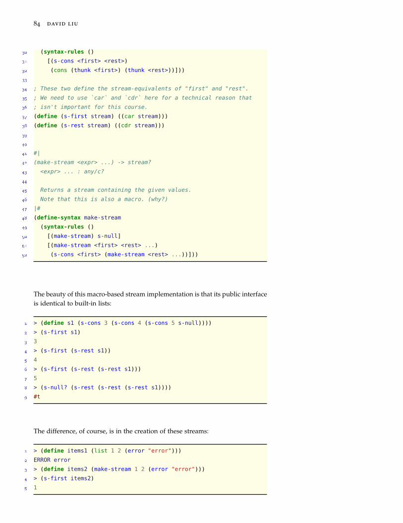
84 david liu
30 (syntax-rules ()
31 [(s-cons <first> <rest>)
32 (cons (thunk <first>) (thunk <rest>))]))
33
34 ; These two define the stream-equivalents of "first" and "rest".
35 ; We need to use `car` and `cdr` here for a technical reason that
36 ; isn't important for this course.
37 (define (s-first stream) ((car stream)))
38 (define (s-rest stream) ((cdr stream)))
39
40
41 #|
42 (make-stream <expr> ...) -> stream?
43 <expr> ... : any/c?
44
45 Returns a stream containing the given values.
46 Note that this is also a macro. (why?)
47 |#
48 (define-syntax make-stream
49 (syntax-rules ()
50 [(make-stream) s-null]
51 [(make-stream <first> <rest> ...)
52 (s-cons <first> (make-stream <rest> ...))]))
The beauty of this macro-based stream implementation is that its public interfaceis identical to built-in lists:
1 > (define s1 (s-cons 3 (s-cons 4 (s-cons 5 s-null))))
2 > (s-first s1)
3 3
4 > (s-first (s-rest s1))
5 4
6 > (s-first (s-rest (s-rest s1)))
7 5
8 > (s-null? (s-rest (s-rest (s-rest s1))))
9 #t
The difference, of course, is in the creation of these streams:
1 > (define items1 (list 1 2 (error "error")))
2 ERROR error
3 > (define items2 (make-stream 1 2 (error "error")))
4 > (s-first items2)
5 1
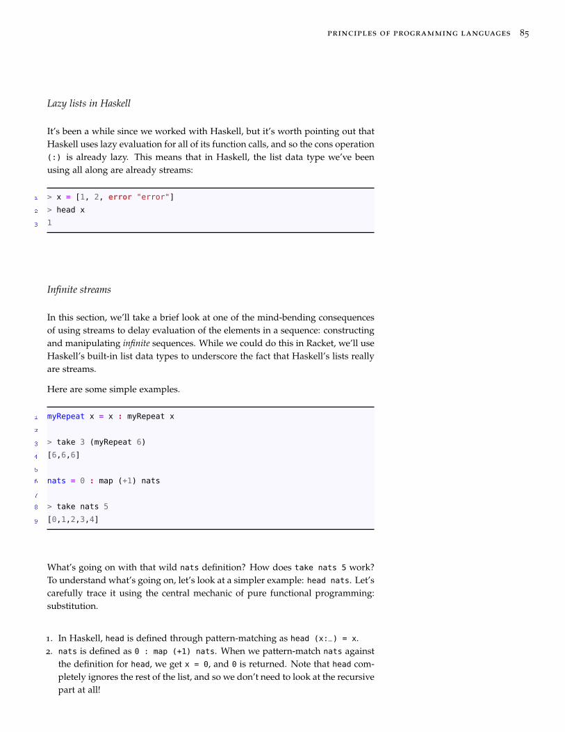
principles of programming languages 85
Lazy lists in Haskell
It’s been a while since we worked with Haskell, but it’s worth pointing out thatHaskell uses lazy evaluation for all of its function calls, and so the cons operation(:) is already lazy. This means that in Haskell, the list data type we’ve beenusing all along are already streams:
1 > x = [1, 2, error "error"]
2 > head x
3 1
Infinite streams
In this section, we’ll take a brief look at one of the mind-bending consequencesof using streams to delay evaluation of the elements in a sequence: constructingand manipulating infinite sequences. While we could do this in Racket, we’ll useHaskell’s built-in list data types to underscore the fact that Haskell’s lists reallyare streams.
Here are some simple examples.
1 myRepeat x = x : myRepeat x
2
3 > take 3 (myRepeat 6)
4 [6,6,6]
5
6 nats = 0 : map (+1) nats
7
8 > take nats 5
9 [0,1,2,3,4]
What’s going on with that wild nats definition? How does take nats 5 work?To understand what’s going on, let’s look at a simpler example: head nats. Let’scarefully trace it using the central mechanic of pure functional programming:substitution.
1. In Haskell, head is defined through pattern-matching as head (x:_) = x.2. nats is defined as 0 : map (+1) nats. When we pattern-match nats against
the definition for head, we get x = 0, and 0 is returned. Note that head com-pletely ignores the rest of the list, and so we don’t need to look at the recursivepart at all!
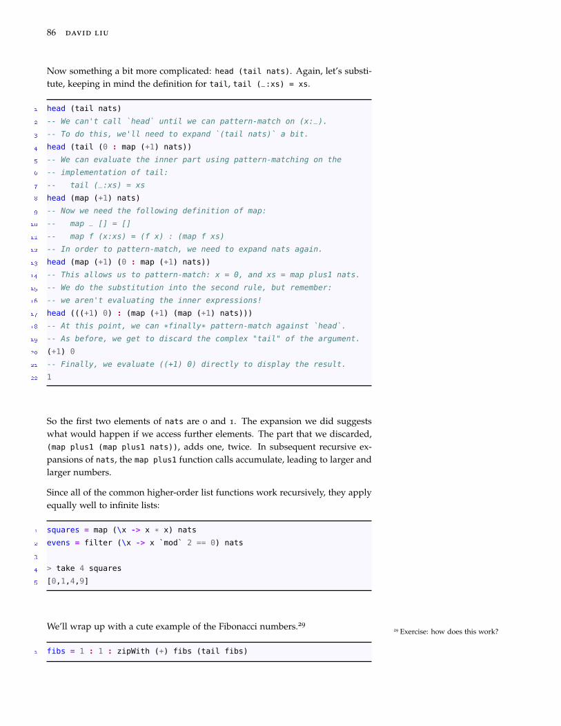
86 david liu
Now something a bit more complicated: head (tail nats). Again, let’s substi-tute, keeping in mind the definition for tail, tail (_:xs) = xs.
1 head (tail nats)
2 -- We can't call `head` until we can pattern-match on (x:_).
3 -- To do this, we'll need to expand `(tail nats)` a bit.
4 head (tail (0 : map (+1) nats))
5 -- We can evaluate the inner part using pattern-matching on the
6 -- implementation of tail:
7 -- tail (_:xs) = xs
8 head (map (+1) nats)
9 -- Now we need the following definition of map:
10 -- map _ [] = []
11 -- map f (x:xs) = (f x) : (map f xs)
12 -- In order to pattern-match, we need to expand nats again.
13 head (map (+1) (0 : map (+1) nats))
14 -- This allows us to pattern-match: x = 0, and xs = map plus1 nats.
15 -- We do the substitution into the second rule, but remember:
16 -- we aren't evaluating the inner expressions!
17 head (((+1) 0) : (map (+1) (map (+1) nats)))
18 -- At this point, we can *finally* pattern-match against `head`.
19 -- As before, we get to discard the complex "tail" of the argument.
20 (+1) 0
21 -- Finally, we evaluate ((+1) 0) directly to display the result.
22 1
So the first two elements of nats are 0 and 1. The expansion we did suggestswhat would happen if we access further elements. The part that we discarded,(map plus1 (map plus1 nats)), adds one, twice. In subsequent recursive ex-pansions of nats, the map plus1 function calls accumulate, leading to larger andlarger numbers.
Since all of the common higher-order list functions work recursively, they applyequally well to infinite lists:
1 squares = map (\x -> x * x) nats
2 evens = filter (\x -> x `mod` 2 == 0) nats
3
4 > take 4 squares
5 [0,1,4,9]
We’ll wrap up with a cute example of the Fibonacci numbers.29
29 Exercise: how does this work?
1 fibs = 1 : 1 : zipWith (+) fibs (tail fibs)
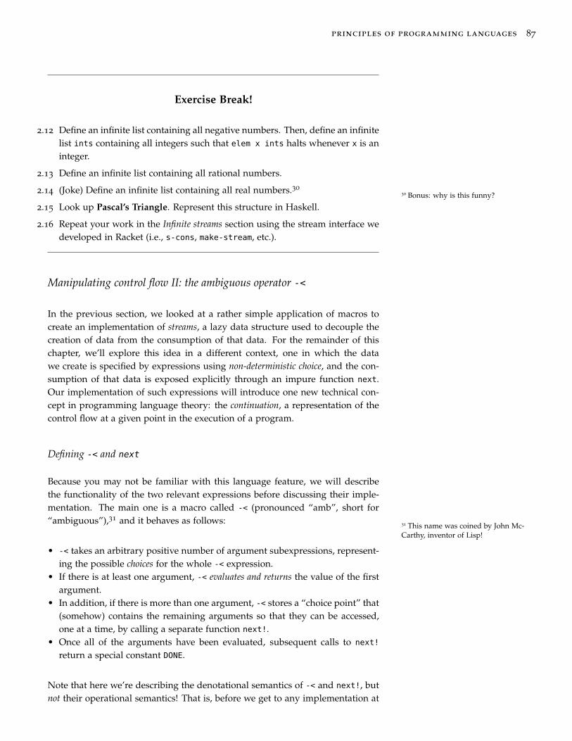
principles of programming languages 87
Exercise Break!
2.12 Define an infinite list containing all negative numbers. Then, define an infinitelist ints containing all integers such that elem x ints halts whenever x is aninteger.
2.13 Define an infinite list containing all rational numbers.
2.14 (Joke) Define an infinite list containing all real numbers.30
30 Bonus: why is this funny?
2.15 Look up Pascal’s Triangle. Represent this structure in Haskell.
2.16 Repeat your work in the Infinite streams section using the stream interface wedeveloped in Racket (i.e., s-cons, make-stream, etc.).
Manipulating control flow II: the ambiguous operator -<
In the previous section, we looked at a rather simple application of macros tocreate an implementation of streams, a lazy data structure used to decouple thecreation of data from the consumption of that data. For the remainder of thischapter, we’ll explore this idea in a different context, one in which the datawe create is specified by expressions using non-deterministic choice, and the con-sumption of that data is exposed explicitly through an impure function next.Our implementation of such expressions will introduce one new technical con-cept in programming language theory: the continuation, a representation of thecontrol flow at a given point in the execution of a program.
Defining -< and next
Because you may not be familiar with this language feature, we will describethe functionality of the two relevant expressions before discussing their imple-mentation. The main one is a macro called -< (pronounced “amb”, short for“ambiguous”),31 and it behaves as follows:
31 This name was coined by John Mc-Carthy, inventor of Lisp!
• -< takes an arbitrary positive number of argument subexpressions, represent-ing the possible choices for the whole -< expression.
• If there is at least one argument, -< evaluates and returns the value of the firstargument.
• In addition, if there is more than one argument, -< stores a “choice point” that(somehow) contains the remaining arguments so that they can be accessed,one at a time, by calling a separate function next!.
• Once all of the arguments have been evaluated, subsequent calls to next!
return a special constant DONE.
Note that here we’re describing the denotational semantics of -< and next!, butnot their operational semantics! That is, before we get to any implementation at
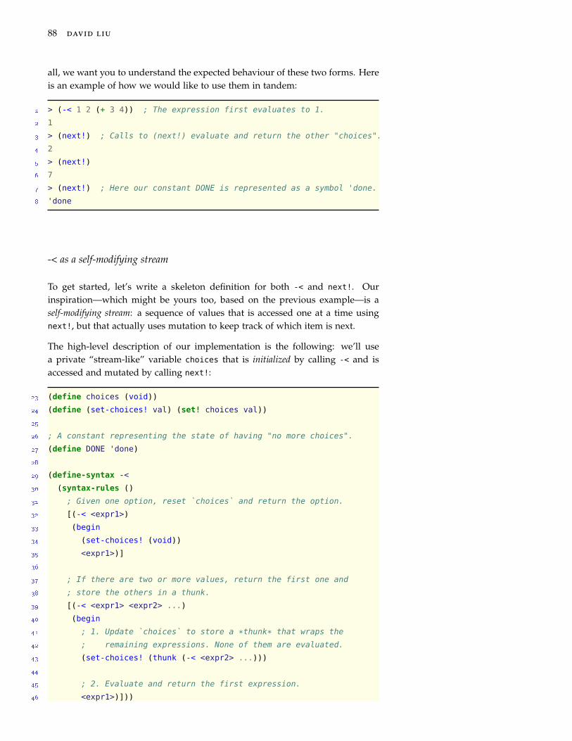
88 david liu
all, we want you to understand the expected behaviour of these two forms. Hereis an example of how we would like to use them in tandem:
1 > (-< 1 2 (+ 3 4)) ; The expression first evaluates to 1.
2 1
3 > (next!) ; Calls to (next!) evaluate and return the other "choices".
4 2
5 > (next!)
6 7
7 > (next!) ; Here our constant DONE is represented as a symbol 'done.
8 'done
-< as a self-modifying stream
To get started, let’s write a skeleton definition for both -< and next!. Ourinspiration—which might be yours too, based on the previous example—is aself-modifying stream: a sequence of values that is accessed one at a time usingnext!, but that actually uses mutation to keep track of which item is next.
The high-level description of our implementation is the following: we’ll usea private “stream-like” variable choices that is initialized by calling -< and isaccessed and mutated by calling next!:
23 (define choices (void))
24 (define (set-choices! val) (set! choices val))
25
26 ; A constant representing the state of having "no more choices".
27 (define DONE 'done)
28
29 (define-syntax -<
30 (syntax-rules ()
31 ; Given one option, reset `choices` and return the option.
32 [(-< <expr1>)
33 (begin
34 (set-choices! (void))
35 <expr1>)]
36
37 ; If there are two or more values, return the first one and
38 ; store the others in a thunk.
39 [(-< <expr1> <expr2> ...)
40 (begin
41 ; 1. Update `choices` to store a *thunk* that wraps the
42 ; remaining expressions. None of them are evaluated.
43 (set-choices! (thunk (-< <expr2> ...)))
44
45 ; 2. Evaluate and return the first expression.
46 <expr1>)]))
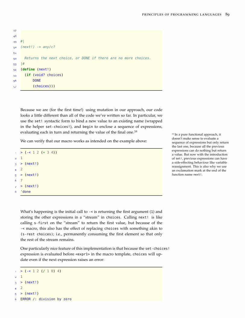
principles of programming languages 89
47
48
49 #|
50 (next!) -> any/c?
51
52 Returns the next choice, or DONE if there are no more choices.
53 |#
54 (define (next!)
55 (if (void? choices)
56 DONE
57 (choices)))
Because we are (for the first time!) using mutation in our approach, our codelooks a little different than all of the code we’ve written so far. In particular, weuse the set! syntactic form to bind a new value to an existing name (wrappedin the helper set-choices!), and begin to enclose a sequence of expressions,evaluating each in turn and returning the value of the final one.32
32 In a pure functional approach, itdoesn’t make sense to evaluate asequence of expressions but only returnthe last one, because all the previousexpressions can do nothing but returna value. But now with the introductionof set!, previous expressions can havea side-effecting behaviour like variablereassignment. This is also why we usean exclamation mark at the end of thefunction name next!.
We can verify that our macro works as intended on the example above:
1 > (-< 1 2 (+ 3 4))
2 1
3 > (next!)
4 2
5 > (next!)
6 7
7 > (next!)
8 'done
What’s happening is the initial call to -< is returning the first argument (1) andstoring the other expressions in a “stream” in choices. Calling next! is likecalling s-first on the “stream” to return the first value, but because of the-< macro, this also has the effect of replacing choices with something akin to(s-rest choices); i.e., permanently consuming the first element so that onlythe rest of the stream remains.
One particularly nice feature of this implementation is that because the set-choices!expression is evaluated before <expr1> in the macro template, choices will up-date even if the next expression raises an error:
1 > (-< 1 2 (/ 1 0) 4)
2 1
3 > (next!)
4 2
5 > (next!)
6 ERROR /: division by zero

90 david liu
7 > (next!)
8 4
This implementation is more complicated than it needs to be, if this were thelimit of what we wanted to achieve. But we aren’t done yet! While this imple-mentation is able to store the other choices, that’s all it saves.
1 > (+ 3 (-< 1 2 (+ 3 4)))
2 4
3 > (next!)
4 2
5 > (next!)
6 7
When the first expression is evaluated, (-< 1 2) returns 1 to the outer expres-sion, which is why the output is 4. However, our implementation sets next! to(thunk (-< 2 (+ 3 4))), and so when it is called, it simply returns 2.
In other words, even though the remaining choices in the choice expression aresaved, the computational context33 in which the expression occurs is not. To fix
33 In the previous example, the “+ 3” isthe computational context.this problem, we’ll need some way of saving this computational context—and
this brings us to the realm of continuations.
Continuations
In our studies to date, we have largely been passive participants in the opera-tional semantics of our languages, subject to the evaluation orders of functioncalls and special syntactic forms. Even with macros, which do allow us to ma-nipulate evaluation order, we have done so only by rewriting expressions intoa fixed set of built-in macros and function calls. However, Racket has a datastructure to directly represent (and hence manipulate) control flow from withina program: the continuation. Consider the following simple expression:
1 (+ (* 3 4) (first (list 1 2 3)))
By now, you should have a very clear sense of how this expression is evaluated,and in particular the order in which the subexpressions are evaluated.34 For each
34 For example, the fact that (* 3 4)
is evaluated before the name first islooked up in the global environment.
subexpression s, we define its continuation to be a representation of what re-mains to be evaluated after s itself has been evaluated. Put another way, thecontinuation of s is a representation of the control flow from immediately after shas been evaluated, up to the final evaluation of the enclosing top-level expres-sion (or enclosing continuation delimiter, a topic we’ll explore later this chap-ter). For example, the continuation of the subexpression (* 3 4) is, in English,“evaluate (first (list 1 2 3)) and then add it to the result.” We represent

principles of programming languages 91
this symbolically using an underscore to represent the “hole” in the remainingexpression: (+ _ (first (list 1 2 3))).35 While it might seem like we can
35 We can also represent the continua-tion as a unary function (lambda (x)
(+ x (first (list 1 2 3)))).determine continuations simply by literally replacing a subexpression with anunderscore, this isn’t exactly true. The continuation of the subexpression (first
(list 1 2 3)) is (+ 12 _); because of left-to-right evaluation order in functioncalls, the (* 3 4) is evaluated before the call to first, and so the continuation ofthe latter call is simply “add 12 to the result.”
Since both identifiers and literal values are themselves expressions, they toohave continuations. The continuation of 4 in the above expression is (+ (* 3_) (first (list 1 2 3))), and the continuation of first is (+ 12 (_ (list 1
2 3))). Finally, the continuation of the whole expression (+ (* 3 4) (first
(list 1 2 3))) is simply “return the value,” which we represent simply as _.
Warning: students often think that an expression’s continuation includes theevaluation of the expression itself, which is incorrect—an expression’s continua-tion represents only the control flow after its evaluation. This is why we replacethe expression with an underscore in the above representation! An easy wayto remember this is that an expression’s continuation doesn’t depend on theexpression itself, but rather the expression’s position in the larger program.
shift: reifying continuations
So far, continuations sound like a rather abstract representation of control flow.What’s quite spectacular about Racket is that it it provides ways to access con-tinuations during the executaion of a program. We say that Racket reifies contin-uations, meaning it exposes continuations as values that a program can accessand manipulate as easily as numbers and lists. We as humans can read a wholeexpression and determine the continuations for each of its subexpressions (likewe did in the previous section). How can we write a program that does this kindof meta-analysis for us?
Though it turns out to be quite possible to implement reified continuationspurely in terms of functions, this is beyond the scope of the course.36 Instead,
36 Those interested should look upcontinuation-passing style.we will use Racket’s syntactic form shift to capture continuations for us.
Note: shift is imported from racket/control; include (require racket/control)
for all code examples in this section.
Here is the relevant syntax pattern:
1 (shift <id> <body> ...)
A shift expression has the following semantics:
1. The current continuation of the shift expression is bound to <id>. By con-vention, we often use k for the <id>.
2. The <body> ... is evaluated (with <id> in scope).

92 david liu
3. The current continuation is discarded, and the value returned is simply thevalue of the last expression in <body> ....
The first two points are pretty straightforward (the binding of the name andevaluation of an expression); the third point is the most surprising, as it causesthe value of the shift expression to “escape” any enclosing expressions.37 Let’s
37 This is similar to using a return deepinside a function body, or raise/throwfor exceptions.
start just by illustrating the second and third points, without worrying about thecontinuation binding.
1 > (shift k (+ 4 5)) ; The shift's body is evaluated and returned.
2 9
3 > (* 100 (shift k (+ 4 5))) ; The shift's continuation, (* 100 _), is discarded!
4 9
Now let’s return to point 1 above; the identifier k is bound to the shift expres-sions continuation. In the first example, this was simply the identity continua-tion (“return the value”), and in the second example, this was the continuation(* 100 _). Of course, just binding the continuation to the name k is not veryuseful. Moreover, k is local to the shift expression, so we cannot refer to it afterthe expression has been evaluated. We’ll use mutation to save the stored contin-uation.38 Note that as in the previous section, shift can take multiple <body>
38 You might have some fun thinkingabout how to approach this and therest of the chapter without using anymutation.
expressions, evaluating each one and returning the value of the last one.
1 > (define saved-cont (void))
2 > (* 100
3 (shift k
4 ; Store the bound continuation in the global variable.
5 (set! saved-cont k)
6 ; Evaluate and return this last expression.
7 (+ 4 5)))
8 9
As expected, when we evaluate the expression, the (* 100 _) is discarded, andthe (+ 4 5) is evaluated and returns. But now we have a global variable storingthe bound continuation—let’s check it out.
1 > saved-cont
2 #<procedure>
Racket stored the continuation (* 100 _) as the unary function (lambda (x) (*100 x))—and we can now call it, just as we would any other function.
1 > (saved-cont 9)
2 900

principles of programming languages 93
Pretty cool! But it seems like shift did something we didn’t want: discard thecurrent continuation. It would be great if we could both store the continuationfor future use, but also not interrupt the regular control flow, so that shift be-haves like other kinds of Racket expressions. This turns out to be quite straight-foward, once we remember that we have access to the current continuation rightin the body of the shift!
1 > (* 100
2 (shift k
3 ; Store the bound continuation in the global variable.
4 (set! saved-cont k)
5 ; Call the current continuation k on the desired argument.
6 (k (+ 4 5))))
7 900
Using continuations in -<
Recall that our motivation for learning about continuations was that our current-< macro implementation stored the choices, but not the computational contextaround each choice. We now have a name for that computational context: it’sjust the continuation of the -< expression! Let’s see how to improve our macrousing shift. Here’s a first attempt, replacing the begin with a shift:
1 (define-syntax -<
2 (syntax-rules ()
3 [(-< <expr1>)
4 (begin
5 (set-choices! (void))
6 <expr1>)]
7
8 [(-< <expr1> <expr2> ...)
9 ; k is bound to the continuation of the (-< ...) expression
10 (shift k
11 (set-choices! (thunk (-< <expr2> ...)))
12 (k <expr1>))]))
For example, in the expression (+ 1 (-< 1 2 3)), k would be bound to (+ 1_).
Of course, our macro is incomplete, as it doesn’t actually “save” k. Doing this isstraight-forward: inside our saved thunk, rather than simply returning the nextchoice (with (-< <expr2> ...)), we call k on the result!39
39 Of course, the mechanism that actu-ally “saves” k is the closure created bythe thunk. Hey, remember those?

94 david liu
31 (define-syntax -<
32 (syntax-rules ()
33 [(-< <expr1>)
34 (begin
35 (set-choices! (void))
36 <expr1>)]
37
38 ; Same as before, except the current continuation is stored in the
39 ; choices thunk!
40 [(-< <expr1> <expr2> ...)
41 (shift k
42 (set-choices! (thunk (k (-< <expr2> ...))))
43 (k <expr1>))]))
And now we get our desired behaviour:
1 > (+ 1 (-< 10 20)) ; `k` is (+ 1 _)
2 11
3 > (next!) ; `choices` is (thunk ((+ 1 _) (-< 20))))
4 21
5 > (next!)
6 'done
It is rather amazing that such a small change unlocks a huge number of possibil-ities for our macro; this truly illustrates the power of continuations and macros.
Using choices as subexpressions
So far, we’ve been focused on the construction of the choices themselves, andchecked our work by calling (next!) at the top-level (in the REPL). But becausethe continuations we’re storing behave as unary functions, we can take the valuereturned and pass them to a larger computation. For example:
1 > (* 100 (-< 1 2))
2 100
3 > (+ 3 (next!))
4 203
This is a pretty useful property that we seem to get “for free”. However, it turnsout that there are two subtle issues with our current implementation that comeup when embedding (next!) inside larger expressions; exploring these willtighten up our implementation and deepen our understanding of continuations.
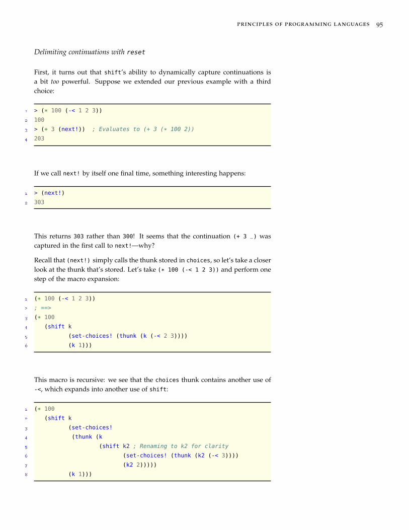
principles of programming languages 95
Delimiting continuations with reset
First, it turns out that shift’s ability to dynamically capture continuations isa bit too powerful. Suppose we extended our previous example with a thirdchoice:
1 > (* 100 (-< 1 2 3))
2 100
3 > (+ 3 (next!)) ; Evaluates to (+ 3 (* 100 2))
4 203
If we call next! by itself one final time, something interesting happens:
1 > (next!)
2 303
This returns 303 rather than 300! It seems that the continuation (+ 3 _) wascaptured in the first call to next!—why?
Recall that (next!) simply calls the thunk stored in choices, so let’s take a closerlook at the thunk that’s stored. Let’s take (* 100 (-< 1 2 3)) and perform onestep of the macro expansion:
1 (* 100 (-< 1 2 3))
2 ; ==>
3 (* 100
4 (shift k
5 (set-choices! (thunk (k (-< 2 3))))
6 (k 1)))
This macro is recursive: we see that the choices thunk contains another use of-<, which expands into another use of shift:
1 (* 100
2 (shift k
3 (set-choices!
4 (thunk (k
5 (shift k2 ; Renaming to k2 for clarity
6 (set-choices! (thunk (k2 (-< 3))))
7 (k2 2)))))
8 (k 1)))
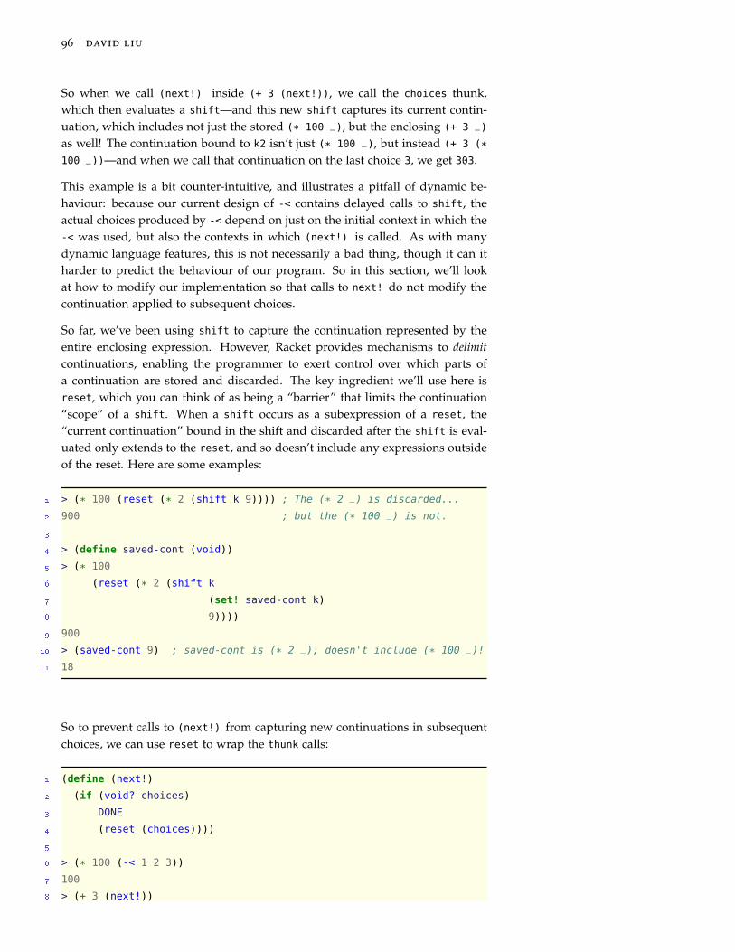
96 david liu
So when we call (next!) inside (+ 3 (next!)), we call the choices thunk,which then evaluates a shift—and this new shift captures its current contin-uation, which includes not just the stored (* 100 _), but the enclosing (+ 3 _)
as well! The continuation bound to k2 isn’t just (* 100 _), but instead (+ 3 (*100 _))—and when we call that continuation on the last choice 3, we get 303.
This example is a bit counter-intuitive, and illustrates a pitfall of dynamic be-haviour: because our current design of -< contains delayed calls to shift, theactual choices produced by -< depend on just on the initial context in which the-< was used, but also the contexts in which (next!) is called. As with manydynamic language features, this is not necessarily a bad thing, though it can itharder to predict the behaviour of our program. So in this section, we’ll lookat how to modify our implementation so that calls to next! do not modify thecontinuation applied to subsequent choices.
So far, we’ve been using shift to capture the continuation represented by theentire enclosing expression. However, Racket provides mechanisms to delimitcontinuations, enabling the programmer to exert control over which parts ofa continuation are stored and discarded. The key ingredient we’ll use here isreset, which you can think of as being a “barrier” that limits the continuation“scope” of a shift. When a shift occurs as a subexpression of a reset, the“current continuation” bound in the shift and discarded after the shift is eval-uated only extends to the reset, and so doesn’t include any expressions outsideof the reset. Here are some examples:
1 > (* 100 (reset (* 2 (shift k 9)))) ; The (* 2 _) is discarded...
2 900 ; but the (* 100 _) is not.
3
4 > (define saved-cont (void))
5 > (* 100
6 (reset (* 2 (shift k
7 (set! saved-cont k)
8 9))))
9 900
10 > (saved-cont 9) ; saved-cont is (* 2 _); doesn't include (* 100 _)!
11 18
So to prevent calls to (next!) from capturing new continuations in subsequentchoices, we can use reset to wrap the thunk calls:
1 (define (next!)
2 (if (void? choices)
3 DONE
4 (reset (choices))))
5
6 > (* 100 (-< 1 2 3))
7 100
8 > (+ 3 (next!))

principles of programming languages 97
9 203
10 > (next!)
11 300
Aborting a computation with shift
Now consider a dual problem:
1 > (* 100 (-< 1 2))
2 100
3 > (+ 3 (next!)) ; Evaluates to (+ 3 (* 100 2))
4 203
If we repeat the call to next! inside a larger expression, we get an error:
1 > (+ 3 (next!))
2 +: contract violation
3 expected: number?
4 given: 'done
5 argument position: 2nd
6 other arguments...:
On the one hand, we should expect this to happen: calling (next!) when thereare no more choices returns our special constant DONE, which cannot be added toa number. On the other, this is pretty annoying: under our current implementa-tion, whenever we embed (next!) inside a larger expression, we either need toguarantee that there is at least one remaining choice, or do an explicit check onwhether the value that’s returned by (next!) is DONE or not before proceedingwith the rest of the computation.
Given this trade-off, we’d like to a way for a call to (next!) to immediatelyreturn DONE, skipping any other computation around the (next!). And as youmight recall from earlier in this chapter, this exact behaviour is provided byshift! So here is the change to our next! implementation:
1 (define (next!)
2 (if (void? choices)
3 (shift k DONE)
4 (reset (choices))))
If there are no more choices, rather than simply return DONE, we instead evaluate(shift k DONE), which causes any surrounding computation to be discarded.40
40 It’s worth repeating here that thisidea of “surrounding computation”is fundamentally dynamic. In thebody of next!, it looks like there’snothing around shift other than theif expression, but the continuationof the shift is determined when it isevaluated, which is in turn determinedby where (next!) is called.

98 david liu
With this change in place, we are able to now call (next!) freely within largerexpressions, and have a 'done “interrupt” the remaining computation.
1 > (* 100 (-< 1 2))
2 100
3 > (+ 3 (next!)) ; Evaluates to (+ 3 (* 100 2))
4 203
5 > (+ 3 (next!)) ; No more error!
6 'done
Branching choices
Even with the improvements of the previous section, we aren’t quite done yet.Our overwriting of choices means that at any time, our program is only awareof one choice point. So in the example below, evaluating the second choiceclobbers the first:
1 > (+ (-< 10 20) (-< 2 3))
2 12
3 > (next!)
4 13
5 > (next!)
6 'done
Now, as programming language designers we might stop here and say, “Well,too bad! You can only use one -< expression per program.” But this is ratherunsatisfying for our users, and so let’s work a little harder to support multiplechoice points. Obviously, just adding more global variables (choices1, choices2,etc.) isn’t an option. We’ll need to be able to represent an arbitrary number ofchoice points, and so a collection-type data structure is most appropriate. Forsimplicity, we’ll use a straightforward one: a stack implemented with a list, withthe front of the list representing the top of the stack:
1 ; choices is now a list of thunks rather than a single thunk.
2 (define choices null)
3 (define (add-choice! c) (push! choices c))
4 (define (get-choice!) (pop! choices))
5
6 ; Push a value onto a stack (add to front of list).
7 (define-syntax push!
8 (syntax-rules ()
9 [(push! <id> obj)
10 (set! <id> (cons obj <id>))]))
11
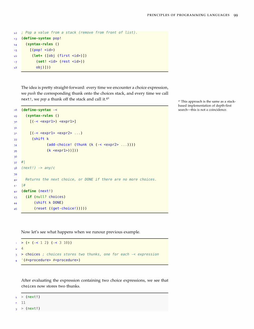
principles of programming languages 99
12 ; Pop a value from a stack (remove from front of list).
13 (define-syntax pop!
14 (syntax-rules ()
15 [(pop! <id>)
16 (let* ([obj (first <id>)])
17 (set! <id> (rest <id>))
18 obj)]))
The idea is pretty straight-forward: every time we encounter a choice expression,we push the corresponding thunk onto the choices stack, and every time we callnext!, we pop a thunk off the stack and call it.41
41 This approach is the same as a stack-based implementation of depth-firstsearch—this is not a coincidence.28 (define-syntax -<
29 (syntax-rules ()
30 [(-< <expr1>) <expr1>]
31
32 [(-< <expr1> <expr2> ...)
33 (shift k
34 (add-choice! (thunk (k (-< <expr2> ...))))
35 (k <expr1>))]))
36
37 #|
38 (next!) -> any/c
39
40 Returns the next choice, or DONE if there are no more choices.
41 |#
42 (define (next!)
43 (if (null? choices)
44 (shift k DONE)
45 (reset ((get-choice!)))))
Now let’s see what happens when we runour previous example.
1 > (+ (-< 1 2) (-< 3 10))
2 4
3 > choices ; choices stores two thunks, one for each -< expression
4 '(#<procedure> #<procedure>)
After evaluating the expression containing two choice expressions, we see thatchoices now stores two thunks.
1 > (next!)
2 11
3 > (next!)
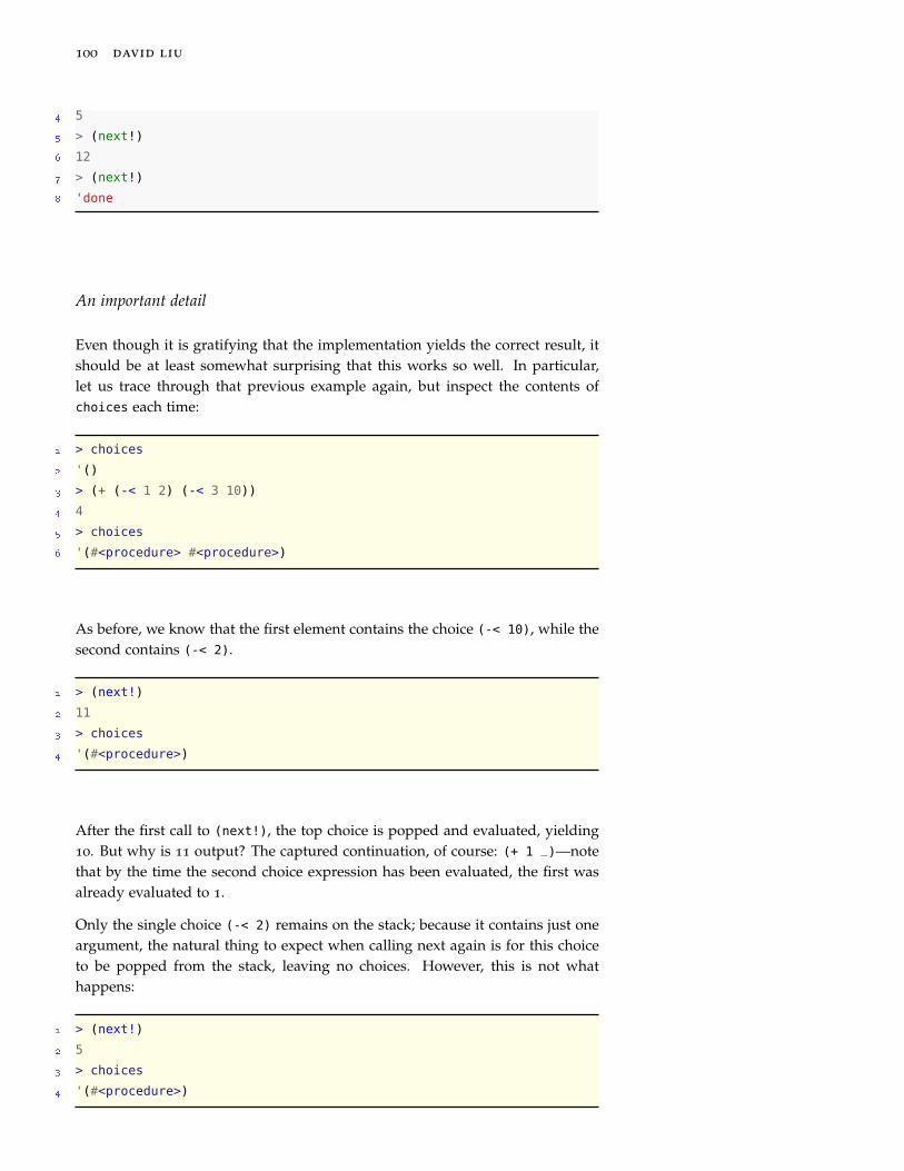
100 david liu
4 5
5 > (next!)
6 12
7 > (next!)
8 'done
An important detail
Even though it is gratifying that the implementation yields the correct result, itshould be at least somewhat surprising that this works so well. In particular,let us trace through that previous example again, but inspect the contents ofchoices each time:
1 > choices
2 '()
3 > (+ (-< 1 2) (-< 3 10))
4 4
5 > choices
6 '(#<procedure> #<procedure>)
As before, we know that the first element contains the choice (-< 10), while thesecond contains (-< 2).
1 > (next!)
2 11
3 > choices
4 '(#<procedure>)
After the first call to (next!), the top choice is popped and evaluated, yielding10. But why is 11 output? The captured continuation, of course: (+ 1 _)—notethat by the time the second choice expression has been evaluated, the first wasalready evaluated to 1.
Only the single choice (-< 2) remains on the stack; because it contains just oneargument, the natural thing to expect when calling next again is for this choiceto be popped from the stack, leaving no choices. However, this is not whathappens:
1 > (next!)
2 5
3 > choices
4 '(#<procedure>)
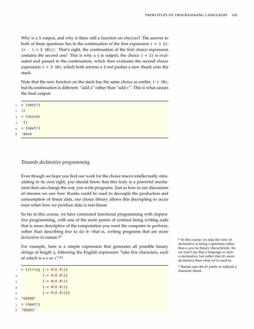
principles of programming languages 101
Why is a 5 output, and why is there still a function on choices? The answer toboth of these questions lies in the continuation of the first expression (-< 1 2):(+ _ (-< 3 10))). That’s right, the continuation of the first choice expressioncontains the second one! This is why a 5 is output; the choice (-< 2) is eval-uated and passed to the continuation, which then evaluates the second choiceexpression (-< 3 10), which both returns a 3 and pushes a new thunk onto thestack.
Note that the new function on the stack has the same choice as earlier, (-< 10),but its continuation is different: “add 2” rather than “add 1”. This is what causesthe final output:
1 > (next!)
2 12
3 > choices
4 '()
5 > (next!)
6 'done
Towards declarative programming
Even though we hope you find our work for the choice macro intellectually stim-ulating in its own right, you should know that this truly is a powerful mecha-nism that can change the way you write programs. Just as how in our discussionof streams we saw how thunks could be used to decouple the production andconsumption of linear data, our choice library allows this decoupling to occureven when how we produce data is non-linear.
So far in this course, we have contrasted functional programming with impera-tive programming, with one of the main points of contrast being writing codethat is more descriptive of the computation you want the computer to perform,rather than describing how to do it—that is, writing programs that are moredeclarative in nature.42
42 In this course, we take the view ofdeclarative as being a spectrum ratherthan a yes/no binary characteristic. Sowe won’t say that a language or styleis declarative, but rather that it’s moredeclarative than what we’re used to.
For example, here is a simple expression that generates all possible binarystrings of length 5, following the English expression “take five characters, eachof which is a 0 or 1”:43
43 Racket uses the #\ prefix to indicate acharacter literal.1 > (string (-< #\0 #\1)
2 (-< #\0 #\1)
3 (-< #\0 #\1)
4 (-< #\0 #\1)
5 (-< #\0 #\1))
6 "00000"
7 > (next!)
8 "00001"

102 david liu
9 > (next!)
10 "00010"
11 > (next!)
12 "00011"
13 > (next!)
14 "00100"
This easy composability is quite remarkable, and is arguably as close to a humanEnglish description as possible.44 Though we can achieve analogous behaviour
44 Modulo the code repetition—see theexercises below for further discussionon that.
with plain higher-order list functions (or nested loops), the simplicity of thisapproach is quite beautiful.
Exercise Break!
2.17 Suppose we tried to generate all binary strings of length 5 by doing the fol-lowing:
1 (let* ([char (-< #\0 #\1)])
2 (string char char char char char))
What does this generate? Explain why. Fix this problem using thunks.
Predicates and backtracking
Generating “all possible combinations” of choices is fun and impressive, but notnecessarily that useful without some kind of mechanism to filter out unwantedcombinations. While we could do this by collecting choices into a stream andapplying a traditional filter operation, we’ll instead take a different approachto combine the automatic generation that choice expressions give us with automaticbacktracking, which is at the core of the technique used by logic programminglanguages like Prolog. The logic programming paradigm is centred on one sim-ple question: “is this true?” Programs are not a sequence of steps to perform,nor the combination of functions; instead, a logic program consists of the defi-nition of a search space (the universe of values known to the program) and thestatement of queries for the computer to answer based on these values. Based onthis description, it is probably not hard to see that logic programs are generallymore declarative than either imperative or functional programs, given that theyfundamentally specify what is being queried, but leave it up to the underlyingimplementation of the language to determine how to answer the query.45
45 A more familiar instance of thisidea is the database query languageSQL, in which programmers writequeries specifying what data they want,without worrying (too much) abouthow this data will be retrieved.
Now, we already have a mechanism for defining a search space, using combina-tions of choices. What about queries? To start, we will define a query operator?-, which takes a unary predicate and an expression, and returns the value ofthe expression if it satisfies the predicate, and DONE if it doesn’t.

principles of programming languages 103
1 (define (?- pred expr)
2 (if (pred expr)
3 expr
4 DONE))
5
6 > (?- even? 10)
7 10
8 > (?- even? -3)
9 'done
Now, all of the work we did in the previous sections pays off: we can call thisfunction with a choice expression!
1 > (?- even? (-< 1 2 3 4))
2 'done
3 > (next!)
4 2
5 > (next!)
6 'done
7 > (next!)
8 'done
When the ?- is originally called, it gets passed the first value in the choiceexpression (i.e., 1); but the continuation of the choice expression is (?- even?_), and so each time next! is called, the next choice gets passed to the query. Touse some terminology of artificial intelligence, calling next! causes backtracking,in which the program goes back to a previous point in its execution, and makesa different choice.
When making queries with choices, it is often the case that we’ll only care aboutthe choices that succeed (i.e., satisfy the predicate), and ignore the others. There-fore it would be nice not to see the intermediate 'done outputs; we can makeone simple change to our predicate to have this available:
1 (define (?- pred expr)
2 (if (pred expr)
3 expr
4 ; Rather than giving up, just try the next choice!
5 (next!)))
6
7 > (?- even? (-< 1 2 3 4))
8 2
9 > (next!)
10 4
11 > (next!)
12 'done
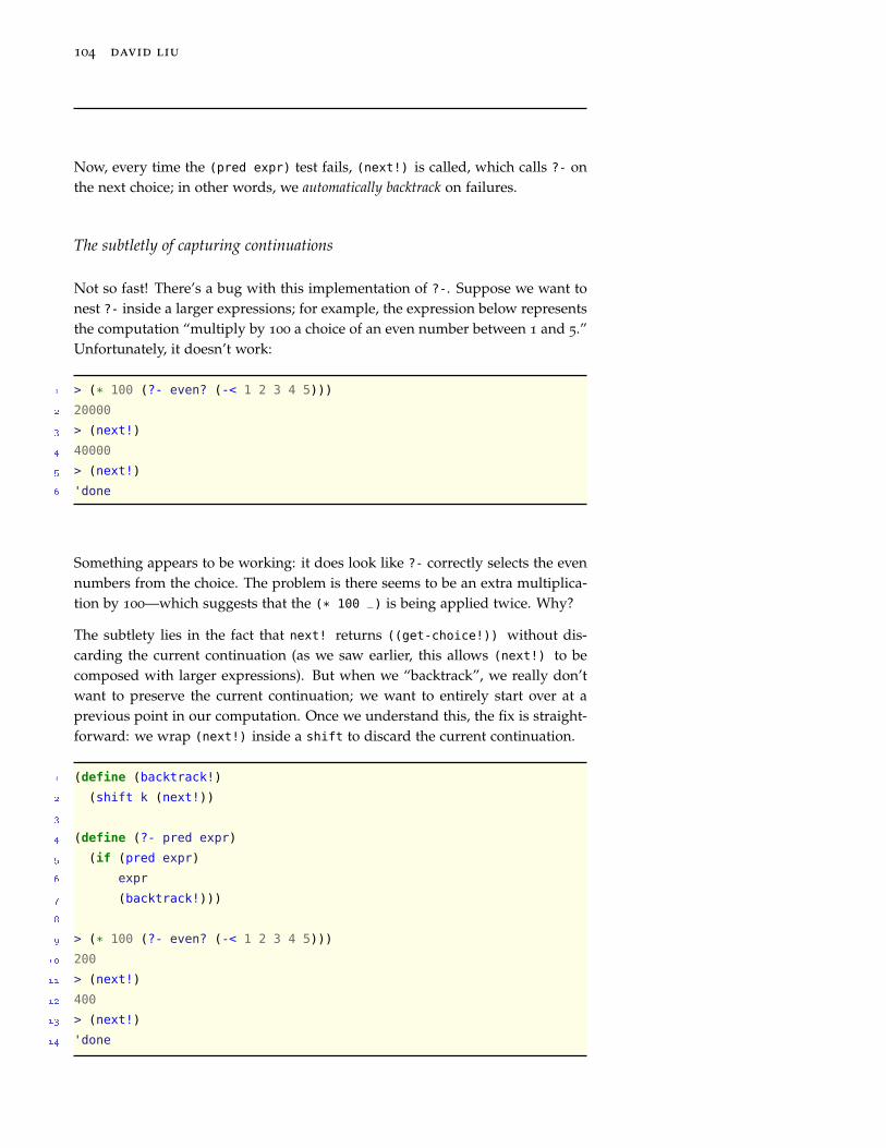
104 david liu
Now, every time the (pred expr) test fails, (next!) is called, which calls ?- onthe next choice; in other words, we automatically backtrack on failures.
The subtletly of capturing continuations
Not so fast! There’s a bug with this implementation of ?-. Suppose we want tonest ?- inside a larger expressions; for example, the expression below representsthe computation “multiply by 100 a choice of an even number between 1 and 5.”Unfortunately, it doesn’t work:
1 > (* 100 (?- even? (-< 1 2 3 4 5)))
2 20000
3 > (next!)
4 40000
5 > (next!)
6 'done
Something appears to be working: it does look like ?- correctly selects the evennumbers from the choice. The problem is there seems to be an extra multiplica-tion by 100—which suggests that the (* 100 _) is being applied twice. Why?
The subtlety lies in the fact that next! returns ((get-choice!)) without dis-carding the current continuation (as we saw earlier, this allows (next!) to becomposed with larger expressions). But when we “backtrack”, we really don’twant to preserve the current continuation; we want to entirely start over at aprevious point in our computation. Once we understand this, the fix is straight-forward: we wrap (next!) inside a shift to discard the current continuation.
1 (define (backtrack!)
2 (shift k (next!))
3
4 (define (?- pred expr)
5 (if (pred expr)
6 expr
7 (backtrack!)))
8
9 > (* 100 (?- even? (-< 1 2 3 4 5)))
10 200
11 > (next!)
12 400
13 > (next!)
14 'done

principles of programming languages 105
Search examples
Probably the easiest way to appreciate the power that this combination of choiceand querying yields is to see some examples in action. We have already seenthe use of this automated backtracking as a lazy filter operation, producingvalues in a list of arguments that satisfy a predicate one at a time, rather thanall at once. We can extend this fairly easily to passing in multiple choice points,with the one downside being that our ?- function only takes unary predicates,and so we’ll need to pass all of the choices into a list of arguments.
Our problem will be the following: given a number n, determine all triples ofnumbers (a, b, c) whose product is n. Here are the definitions of the inputdata and predicate we’ll use.
7 #|
8 (num-between start end) -> integer?
9 start: integer?
10 end: integer?
11 Precondition: start < end
12 Returns a choice of a number in the range [start..end - 1], inclusive.
13 |#
14 (define (num-between start end)
15 (if (equal? start (- end 1))
16 (-< start)
17 (-< start (num-between (+ 1 start) end))))
18
19 #|
20 (triples n) -> (listof integer?)
21 n: integer?
22
23 Returns a choice of a list of three integers between 1 and n, inclusive.
24 |#
25 (define (triples n)
26 (list (num-between 1 (+ n 1))
27 (num-between 1 (+ n 1))
28 (num-between 1 (+ n 1))))
29
30 #|
31 (product? n) -> (-> (listof integer?) boolean?)
32 n: integer?
33
34 Returns a predicate that takes a list of integers and returns whether
35 their product is n.
36 |#
37 (define (product? n)
38 (lambda (triple)
39 (equal? n (apply * triple))))
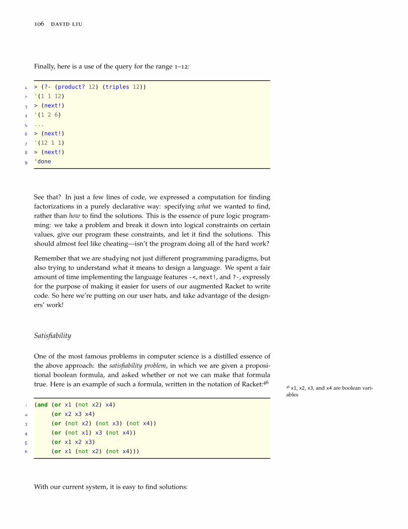
106 david liu
Finally, here is a use of the query for the range 1–12:
1 > (?- (product? 12) (triples 12))
2 '(1 1 12)
3 > (next!)
4 '(1 2 6)
5 ...
6 > (next!)
7 '(12 1 1)
8 > (next!)
9 'done
See that? In just a few lines of code, we expressed a computation for findingfactorizations in a purely declarative way: specifying what we wanted to find,rather than how to find the solutions. This is the essence of pure logic program-ming: we take a problem and break it down into logical constraints on certainvalues, give our program these constraints, and let it find the solutions. Thisshould almost feel like cheating—isn’t the program doing all of the hard work?
Remember that we are studying not just different programming paradigms, butalso trying to understand what it means to design a language. We spent a fairamount of time implementing the language features -<, next!, and ?-, expresslyfor the purpose of making it easier for users of our augmented Racket to writecode. So here we’re putting on our user hats, and take advantage of the design-ers’ work!
Satisfiability
One of the most famous problems in computer science is a distilled essence ofthe above approach: the satisfiability problem, in which we are given a proposi-tional boolean formula, and asked whether or not we can make that formulatrue. Here is an example of such a formula, written in the notation of Racket:46
46 x1, x2, x3, and x4 are boolean vari-ables
1 (and (or x1 (not x2) x4)
2 (or x2 x3 x4)
3 (or (not x2) (not x3) (not x4))
4 (or (not x1) x3 (not x4))
5 (or x1 x2 x3)
6 (or x1 (not x2) (not x4)))
With our current system, it is easy to find solutions:

principles of programming languages 107
1 (define (sat lst)
2 (let ([x1 (first lst)]
3 [x2 (second lst)]
4 [x3 (third lst)]
5 [x4 (fourth lst)])
6 (and (or x1 (not x2) x4)
7 (or x2 x3 x4)
8 (or (not x2) (not x3) (not x4))
9 (or (not x1) x3 (not x4))
10 (or x1 x2 x3)
11 (or x1 (not x2) (not x4)))))
12
13 > (?- sat (list (-< #t #f)
14 (-< #t #f)
15 (-< #t #f)
16 (-< #t #f)))
17 '(#t #t #t #f)
18 > (next!)
19 '(#t #t #f #f)
20 > (next!)
21 '(#t #f #t #t)
22 > (next!)
23 '(#t #f #t #f)
24 > (next!)
25 '(#f #f #t #t)
26 > (next!)
27 '(#f #f #t #f)
28 > (next!)
29 'done


3 Type systems
I conclude that there are two waysof constructing a software design:One way is to make it so simplethat there are obviously nodeficiencies and the other way is tomake it so complicated that thereare no obvious deficiencies.
Tony Hoare
Here is a problematic Racket function.
1 (define (f x)
2 (+ x (first x)))
Calling this function on any input will fail, due to a type error: the parameter x
cannot simultaneously be a number (to be a valid argument to +) and a list (tobe a valid argument to first). Our goal for this chapter is to study type systemsimplemented by different programming languages. While you certainly have anintuitive notion of types coming from past programming experience, you maynot yet have appreciated the complex design decisions that go into how types arerepresented and used in a programming language, and how differences in thesedecisions can have major impacts on the programs written in these languages.
We start with a few definitions to make sure we’re on the same page. A typeis a set of values together with a set of behaviours on those values. Note thatthis is a pretty abstract notion that differs among programming languages: aninteger in Racket can take on a different set of values than an int in C,1 and
1 Try adding two very large integers ineach language!the built-in String functions in Haskell are different from the String methods
in Java. But what is common to all of these languages is the notion of whatinformation a type conveys: if we say that an expression E has type “integer”,this constrains both the possible values we expect that expression to have (i.e.,what its denotational meaning is), and how we can use this expression in thecontext of a large program (e.g., (+ 1 E) is okay but E[10] is not). A type systemis the set of rules in a programming language governing the semantics of typesin the language. This includes how types are defined, the syntax rules governingwhere and how types can be written, and how types affect the operational and
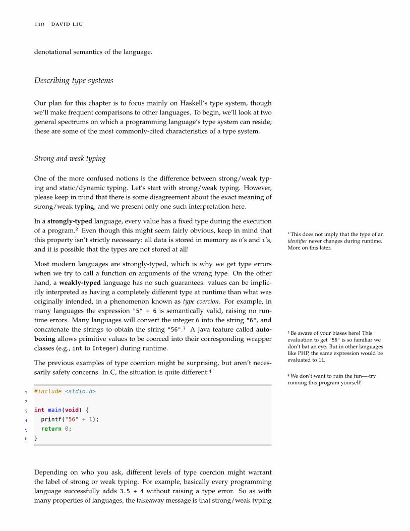
110 david liu
denotational semantics of the language.
Describing type systems
Our plan for this chapter is to focus mainly on Haskell’s type system, thoughwe’ll make frequent comparisons to other languages. To begin, we’ll look at twogeneral spectrums on which a programming language’s type system can reside;these are some of the most commonly-cited characteristics of a type system.
Strong and weak typing
One of the more confused notions is the difference between strong/weak typ-ing and static/dynamic typing. Let’s start with strong/weak typing. However,please keep in mind that there is some disagreement about the exact meaning ofstrong/weak typing, and we present only one such interpretation here.
In a strongly-typed language, every value has a fixed type during the executionof a program.2 Even though this might seem fairly obvious, keep in mind that
2 This does not imply that the type of anidentifier never changes during runtime.More on this later.
this property isn’t strictly necessary: all data is stored in memory as 0’s and 1’s,and it is possible that the types are not stored at all!
Most modern languages are strongly-typed, which is why we get type errorswhen we try to call a function on arguments of the wrong type. On the otherhand, a weakly-typed language has no such guarantees: values can be implic-itly interpreted as having a completely different type at runtime than what wasoriginally intended, in a phenomenon known as type coercion. For example, inmany languages the expression "5" + 6 is semantically valid, raising no run-time errors. Many languages will convert the integer 6 into the string "6", andconcatenate the strings to obtain the string "56".3 A Java feature called auto-
3 Be aware of your biases here! Thisevaluation to get "56" is so familiar wedon’t bat an eye. But in other languageslike PHP, the same expression would beevaluated to 11.
boxing allows primitive values to be coerced into their corresponding wrapperclasses (e.g., int to Integer) during runtime.
The previous examples of type coercion might be surprising, but aren’t neces-sarily safety concerns. In C, the situation is quite different:4
4 We don’t want to ruin the fun—-tryrunning this program yourself!
1 #include <stdio.h>
2
3 int main(void) {
4 printf("56" + 1);
5 return 0;
6 }
Depending on who you ask, different levels of type coercion might warrantthe label of strong or weak typing. For example, basically every programminglanguage successfully adds 3.5 + 4 without raising a type error. So as withmany properties of languages, the takeaway message is that strong/weak typing

principles of programming languages 111
is not a binary property, but a set of nuanced rules about what types can becoerced and when. It goes without saying that mastering these rules is importantfor facility in any programming language.
Static and dynamic typing
Even assuming that we are in a very strongly-typed language with little or notype coercion, there is still the fundamental question of “when does the pro-gram know about (and check) types?” The answer to this question is one of thekey characteristics of a programming language, as it deeply influences both thelanguage’s semantics and the implementation of any interpreter or compiler forthat language.
In statically-typed languages, the type of every expression is determined di-rectly from the source code, before any code is actually executed. In languages thatpermit mutation, static typing requires that even as variables change values, theycan only change to values within the same type. Most of these languages requirean explicit type to be specified at the declaration of each variable, although aswe’ll discuss later, this is not an absolute requirement for static typing.
In contrast, dynamically-typed languages do not perform any type-checkinguntil the program is run. In such languages, a type error is a runtime error—inthe same category as division by zero or array out-of-bounds errors.
As we mentioned earlier, types really form a collection of constraints on pro-grams, so it shouldn’t come as a surprise that static typing is really a form ofprogram verification (like proving program correctness from CSC236). If a com-piler can check that nowhere in the code does a variable take on a different type,we are guaranteed that at no point in the program’s runtime does that variabletake on a different type. By checking the types of all expressions, variables,and functions, the compiler is able to detect code errors (such as invalid func-tion calls) before any code is run at all. Moreover, static type analysis can besometimes used as a compiler optimization: if we have compile-time guaranteesabout the types of all expressions during the program’s run, we can then dropthe runtime type checks when functions are called. As we’ll discuss in the nextsection, statically-typed languages perform type checking before programs arerun, essentially rejecting certain programs because they have type errors. Thissounds great, and it very often is. However, type systems gain their power byenforcing type constraints; the stricter the constraints, the more erroneous pro-grams can be rejected. This can also have the consequence of rejecting perfectlycorrect programs5 that do not satisfy these constraints. However, it’s also worth
5 We’ll see a few examples of this whenwe study Haskell’s type system in thenext section.
pointing out that most statically-typed languages have a way of “escaping” thetype system with a universal type like Object or Any, and in this way allow oneto write code without any type constraints.

112 david liu
The basics of Haskell’s type system
In Haskell, types are denoted by capitalized names like Bool, Char, and Integer.In the Haskell interpreter, you can see the type of any expression with :type,or :t for short. Some examples follow; since Haskell’s numeric types are a bitcomplex, we’re deferring them until later.
1 > :t True
2 True :: Bool
3 > :t 'a'
4 'a' :: Char
5 > :t "Hello"
6 "Hello" :: [Char]
Note that the square brackets surrounding the Char indicates a list: like C,Haskell interprets strings simply as a list of characters.6 One important dif-
6 Haskell also provides a type synonym(i.e., alias) for [Char] called String.ference between Haskell and Racket is that lists must contain values of the same
type, so the expression [True, 'a'] is rejected by Haskell. A similar restrictionalso applies to if expressions: both the then and else subexpressions must havethe same type:
1 > :t (if 3 > 1 then "hi" else "bye")
2 (if 3 > 1 then "hi" else "bye") :: [Char]
The above example illustrates the static nature of Haskell’s type-checking: thetype of the entire if expression is given, without evaluating it! Haskell cando this precisely because of the aforementioned restriction: because the Haskellcompiler knows that both branches evaluate to strings, it is able to determinethat the type of the overall expression is a string without knowing which branchwould actually be evaluated!
Function types and currying
In Haskell, all functions have a type that can be inspected in the same way.
1 > :t not
2 not :: Bool -> Bool
The type signature Bool -> Bool means that not is a function that takes as in-put a Bool value, and then returns a Bool value. The very existence of a typesignature for a function has huge implications for how functions can be used.For instance, functions in Haskell must have a fixed number of arguments, fixedtypes for all their arguments, and one fixed return type. Contrast this withRacket’s member function, which returns either a list or #f (a boolean).

principles of programming languages 113
What about functions that take in two parameters? For example, what is thetype of the “and” function (&&)?
1 > :t (&&)
2 (&&) :: Bool -> Bool -> Bool
Huh, that’s weird. One probably would have expected something like (Bool,
Bool) -> Bool to denote that this function takes in two arguments. So whatdoes Bool -> Bool -> Bool actually mean? The -> operator in Haskell is right-associative, which means that the proper grouping of that signature is Bool
-> (Bool -> Bool). This is quite suggestive: Haskell interprets (&&) as a unaryhigher-order function that returns a function with type Bool -> Bool! This is thegreat insight from the lambda calculus known as currying: any multi-parameterfunction can be broken down into a nested composition of single-valued func-tions.7
7 An observant reader might have no-ticed that the syntactic rules in thePrologue for generating lambda cal-culus expressions did not contain anymention of multi-parameter functions.This is because currying makes it possi-ble to express such functions within thesingle-parameter syntax.
Consider the following function definition, which you can think of as a partialapplication of (&&):
1 newF y = (&&) True y
The type of newF is certainly Bool -> Bool: if y is True then the function evalu-ates to True, and if y is False then the expression is False. By fixing the valueof the first argument to (&&), we have created a new function. But in fact they is completely unnecessary to defining newF, and the following definition iscompletely equivalent.
1 newF = (&&) True
This makes sense when we think in terms of referential transparency: every timewe see an expression like newF True, we can substitute this definition of newF toobtain the completely equivalent expression (&&) True True.
It turns out that Haskell treats all functions as unary functions, and that functionapplication is indicated by simply separating two expressions with a space. Anexpression like (&&) False True might look like a single function application ontwo arguments, but the true syntactic form parsed by Haskell is ((&&) False)
True,8 where ((&&) False) is evaluated to create a new function, which is then8 function application is left-associative
applied to True. In other words, the following definitions of (&&) are equivalent:
1 -- Usual definition
2 (&&) x y = if x then y else False
3 -- As a higher-order function
4 (&&) x = \y -> if x then y else False
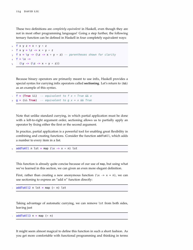
114 david liu
These two definitions are completely equivalent in Haskell, even though they arenot in most other programming languages! Going a step further, the followingternary function can be defined in Haskell in four completely equivalent ways:
1 f x y z = x + y * z
2 f x y = \z -> x + y * z
3 f x = \y -> (\z -> x + y * z) -- parentheses shown for clarity
4 f = \x ->
5 (\y -> (\z -> x + y * z))
Because binary operators are primarily meant to use infix, Haskell provides aspecial syntax for currying infix operators called sectioning. Let’s return to (&&)
as an example of this syntax.
1 f = (True &&) -- equivalent to f x = True && x
2 g = (&& True) -- equivalent to g x = x && True
Note that unlike standard currying, in which partial application must be donewith a left-to-right argument order, sectioning allows us to partially apply anoperator by fixing either the first or the second argument.
In practice, partial application is a powerful tool for enabling great flexibility incombining and creating functions. Consider the function addToAll, which addsa number to every item in a list.
1 addToAll n lst = map (\x -> x + n) lst
This function is already quite concise because of our use of map, but using whatwe’ve learned in this section, we can given an even more elegant definition.
First, rather than creating a new anonymous function (\x -> x + n), we canuse sectioning to express an “add n” function directly:
1 addToAll2 n lst = map (+ n) lst
Taking advantage of automatic currying, we can remove lst from both sides,leaving just
1 addToAll3 n = map (+ n)
It might seem almost magical to define this function in such a short fashion. Asyou get more comfortable with functional programming and thinking in terms

principles of programming languages 115
of combining and creating functions, you can interpret the final definition quiteelegantly as “addToAll3 maps the ‘add n’ function.”
Defining types in Haskell
Now that we have been introduced to Haskell’s type system, we’ll study how todefine our own types in this language.
The running example we’ll use in this section is a set of types representingsimple geometric objects. There’s quite a bit of new terminology in this section,so make sure you read carefully! First, a point (x,y) in the Cartesian plane canbe represented by the following Point type.
1 data Point = Point Float Float
You can probably guess what this does: on the left side, we are defining a newtype Point using the data keyword. On the right, we define how to createinstances of this type; the Point is a value constructor, which takes two Float
arguments and returns a value of type Point. Let’s play around with this newtype.
1 > p = Point 3 4
2 > :t p
3 p :: Point
4 > :t Point
5 Point :: Float -> Float -> Point
There is a common source of confusion when it comes to Haskell’s treatmentof types that we are going to confront head-on. In Haskell, there is a strictseparation between the expression language used to define names and evaluateexpressions, and the type language used to represent the types of these expres-sions. We have seen some artifacts of this separation already: for example, the-> operator is used in expressions as part of the syntax for a lambda expression,and in types to represent a function type. We have also seen the mingling ofthese in type annotations, which come in the form <expression> :: <type>.
A type declaration is a different instance of this mingling. In our above example,the Point on the left is the name of a new type, while the Point on the right isthe name of a function that returns values of that type. In typical object-orientedlanguages, the constructor of a class is a special method, and its significance isenforced semantically (in part) by having its name be the same as the class name.This is actually not true in Haskell, as we illustrate below:
1 -- Point is the type and MyPoint is its constructor.
2 data Point = MyPoint Float Float
3
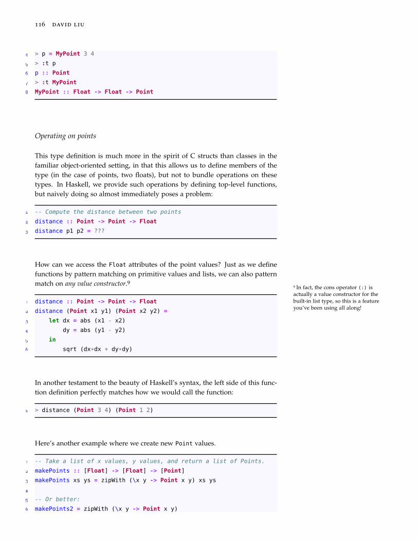
116 david liu
4 > p = MyPoint 3 4
5 > :t p
6 p :: Point
7 > :t MyPoint
8 MyPoint :: Float -> Float -> Point
Operating on points
This type definition is much more in the spirit of C structs than classes in thefamiliar object-oriented setting, in that this allows us to define members of thetype (in the case of points, two floats), but not to bundle operations on thesetypes. In Haskell, we provide such operations by defining top-level functions,but naively doing so almost immediately poses a problem:
1 -- Compute the distance between two points
2 distance :: Point -> Point -> Float
3 distance p1 p2 = ???
How can we access the Float attributes of the point values? Just as we definefunctions by pattern matching on primitive values and lists, we can also patternmatch on any value constructor.9
9 In fact, the cons operator (:) isactually a value constructor for thebuilt-in list type, so this is a featureyou’ve been using all along!
1 distance :: Point -> Point -> Float
2 distance (Point x1 y1) (Point x2 y2) =
3 let dx = abs (x1 - x2)
4 dy = abs (y1 - y2)
5 in
6 sqrt (dx*dx + dy*dy)
In another testament to the beauty of Haskell’s syntax, the left side of this func-tion definition perfectly matches how we would call the function:
1 > distance (Point 3 4) (Point 1 2)
Here’s another example where we create new Point values.
1 -- Take a list of x values, y values, and return a list of Points.
2 makePoints :: [Float] -> [Float] -> [Point]
3 makePoints xs ys = zipWith (\x y -> Point x y) xs ys
4
5 -- Or better:
6 makePoints2 = zipWith (\x y -> Point x y)
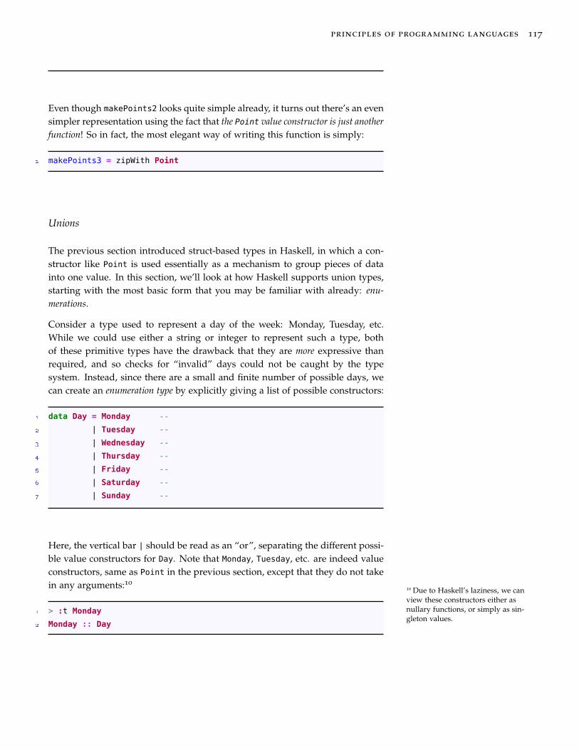
principles of programming languages 117
Even though makePoints2 looks quite simple already, it turns out there’s an evensimpler representation using the fact that the Point value constructor is just anotherfunction! So in fact, the most elegant way of writing this function is simply:
1 makePoints3 = zipWith Point
Unions
The previous section introduced struct-based types in Haskell, in which a con-structor like Point is used essentially as a mechanism to group pieces of datainto one value. In this section, we’ll look at how Haskell supports union types,starting with the most basic form that you may be familiar with already: enu-merations.
Consider a type used to represent a day of the week: Monday, Tuesday, etc.While we could use either a string or integer to represent such a type, bothof these primitive types have the drawback that they are more expressive thanrequired, and so checks for “invalid” days could not be caught by the typesystem. Instead, since there are a small and finite number of possible days, wecan create an enumeration type by explicitly giving a list of possible constructors:
1 data Day = Monday --
2 | Tuesday --
3 | Wednesday --
4 | Thursday --
5 | Friday --
6 | Saturday --
7 | Sunday --
Here, the vertical bar | should be read as an “or”, separating the different possi-ble value constructors for Day. Note that Monday, Tuesday, etc. are indeed valueconstructors, same as Point in the previous section, except that they do not takein any arguments:10
10 Due to Haskell’s laziness, we canview these constructors either asnullary functions, or simply as sin-gleton values.
1 > :t Monday
2 Monday :: Day

118 david liu
This use of alternative constructors in Haskell is pretty standard in other lan-guages as well. What is more unusual is Haskell’s ability to combine constructorsthat take arguments with alternatives to declare types that have radically differentforms:
1 data Shape
2 = Circle Point Float -- ^ centre and radius
3 | Rectangle Point Point -- ^ top-left and bottom-right corners
Here it is really important to get the terminology correct. This code createsa new type Shape, which has two value constructors: Circle and Rectangle.Here’s how we might use this new type.11
11 Remember: Circle and Rectangle arefunctions, while Shape is a type.
1 > shape = Circle (Point 3 4) 1
2 > :t shape
3 shape :: Shape
4 > :t [Circle (Point 3 4) 5, Rectangle (Point 0 0) (Point 1 1)]
5 [Circle (Point 3 4) 5, Rectangle (Point 0 0) (Point 1 1)] :: [Shape]
Here’s another example of using pattern-matching to write a function operatingon Shapes. Note that each constructor gets its own pattern-match rule, and wecan even nest patterns.
1 area :: Shape -> Float
2 area (Circle _ r) = pi * r * r
3 area (Rectangle (Point x1 y1) (Point x2 y2)) =
4 abs ((x2-x1) * (y2-y1))
5
6 > area (Circle (Point 3 4) 1)
7 3.141592653589793
8 > area (Rectangle (Point 4 5) (Point 6 2))
9 6.0
Unions in C
You might be familiar with struct and union types in C, which together ap-proximate algebraic data types from Haskell. That said, the C syntax is quite abit more verbose. And for unions, there is additional legwork required of pro-grammers to keep track of what part of the union is active. Here is how ourShape example might look in C. Note that the circle and rectangle memberswill overlap in memory: only one of them is available at a time.
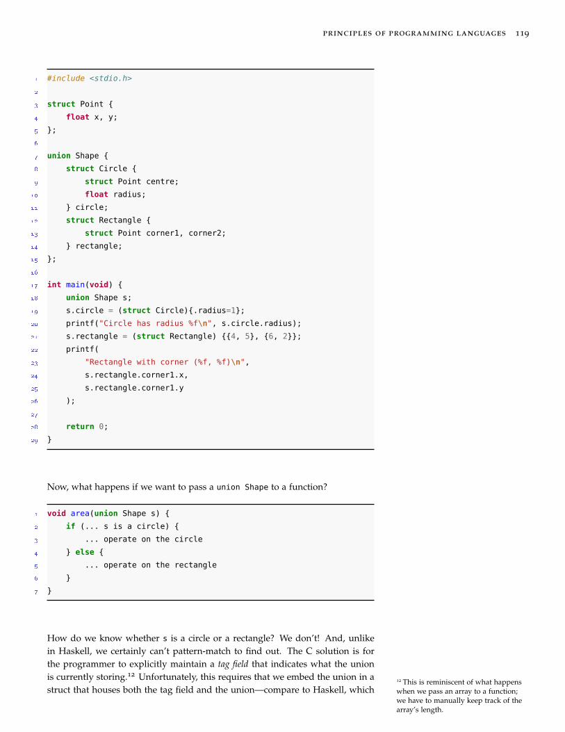
principles of programming languages 119
1 #include <stdio.h>
2
3 struct Point {
4 float x, y;
5 };
6
7 union Shape {
8 struct Circle {
9 struct Point centre;
10 float radius;
11 } circle;
12 struct Rectangle {
13 struct Point corner1, corner2;
14 } rectangle;
15 };
16
17 int main(void) {
18 union Shape s;
19 s.circle = (struct Circle){.radius=1};
20 printf("Circle has radius %f\n", s.circle.radius);
21 s.rectangle = (struct Rectangle) {{4, 5}, {6, 2}};
22 printf(
23 "Rectangle with corner (%f, %f)\n",
24 s.rectangle.corner1.x,
25 s.rectangle.corner1.y
26 );
27
28 return 0;
29 }
Now, what happens if we want to pass a union Shape to a function?
1 void area(union Shape s) {
2 if (... s is a circle) {
3 ... operate on the circle
4 } else {
5 ... operate on the rectangle
6 }
7 }
How do we know whether s is a circle or a rectangle? We don’t! And, unlikein Haskell, we certainly can’t pattern-match to find out. The C solution is forthe programmer to explicitly maintain a tag field that indicates what the unionis currently storing.12 Unfortunately, this requires that we embed the union in a
12 This is reminiscent of what happenswhen we pass an array to a function;we have to manually keep track of thearray’s length.
struct that houses both the tag field and the union—compare to Haskell, which

120 david liu
keeps track of all of this for us!
1 #include <stdio.h>
2 #include <math.h>
3 #define pi 3.141592653589793
4
5 struct Point {
6 float x, y;
7 };
8
9 struct Shape {
10 enum {CIRCLE, RECTANGLE} shape_tag;
11 union {
12 struct Circle {
13 struct Point centre;
14 float radius;
15 } circle;
16 struct Rectangle {
17 struct Point corner1, corner2;
18 } rectangle;
19 } shape;
20 };
21
22 float area(struct Shape s) {
23 if (s.shape_tag == CIRCLE) {
24 float r = s.shape.circle.radius;
25 return pi * r * r;
26 } else { // rectangle
27 float x1 = s.shape.rectangle.corner1.x;
28 float y1 = s.shape.rectangle.corner1.y;
29 float x2 = s.shape.rectangle.corner2.x;
30 float y2 = s.shape.rectangle.corner2.y;
31 return abs ((x2-x1) * (y2-y1));
32 }
33 }
34
35 int main(void) {
36 struct Shape s;
37 s.shape_tag = CIRCLE;
38 s.shape.circle = (struct Circle){.radius=1};
39 printf("%f\n", area(s));
40 s.shape_tag = RECTANGLE;
41 s.shape.rectangle = (struct Rectangle) {{4, 5}, {6, 2}};
42 printf("%f\n", area(s));
43
44 return 0;
45 }
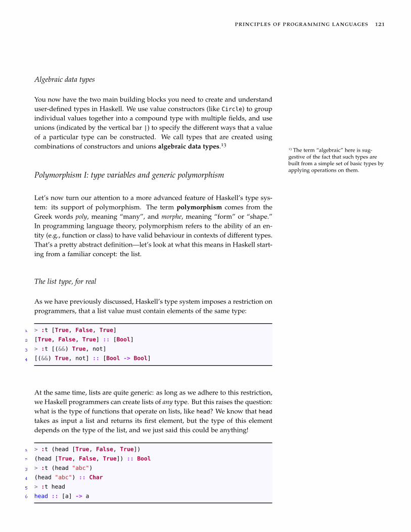
principles of programming languages 121
Algebraic data types
You now have the two main building blocks you need to create and understanduser-defined types in Haskell. We use value constructors (like Circle) to groupindividual values together into a compound type with multiple fields, and useunions (indicated by the vertical bar |) to specify the different ways that a valueof a particular type can be constructed. We call types that are created usingcombinations of constructors and unions algebraic data types.13
13 The term “algebraic” here is sug-gestive of the fact that such types arebuilt from a simple set of basic types byapplying operations on them.
Polymorphism I: type variables and generic polymorphism
Let’s now turn our attention to a more advanced feature of Haskell’s type sys-tem: its support of polymorphism. The term polymorphism comes from theGreek words poly, meaning “many”, and morphe, meaning “form” or “shape.”In programming language theory, polymorphism refers to the ability of an en-tity (e.g., function or class) to have valid behaviour in contexts of different types.That’s a pretty abstract definition—let’s look at what this means in Haskell start-ing from a familiar concept: the list.
The list type, for real
As we have previously discussed, Haskell’s type system imposes a restriction onprogrammers, that a list value must contain elements of the same type:
1 > :t [True, False, True]
2 [True, False, True] :: [Bool]
3 > :t [(&&) True, not]
4 [(&&) True, not] :: [Bool -> Bool]
At the same time, lists are quite generic: as long as we adhere to this restriction,we Haskell programmers can create lists of any type. But this raises the question:what is the type of functions that operate on lists, like head? We know that headtakes as input a list and returns its first element, but the type of this elementdepends on the type of the list, and we just said this could be anything!
1 > :t (head [True, False, True])
2 (head [True, False, True]) :: Bool
3 > :t (head "abc")
4 (head "abc") :: Char
5 > :t head
6 head :: [a] -> a

122 david liu
The type of head is [a] -> a. This differs from all other type signatures wehave seen so far because it contains a type variable a.14 A type variable is an
14 In type expressions, type variablesmust start with a lowercase letter,distinguishing them from types them-selves.
identifier in a type expression that can be instantiated to any type, such as Bool
or Char. This type signature tells us that head works on any type of the form [a],and returns a value of type a. Each time we call head, we match the parametertype [a] against the type of the argument, and use this to instantiate the typevariable a to a concrete type to do the type-checking. For example, here is whathappens when we type-check the expression head [True, False, True]:
1. Haskell determines that the type of the argument list is [Bool].2. Haskell matches the argument type [Bool] against the parameter type [a],
and instantiates a = Bool in the function type.3. Haskell takes the return type a, with a instantiated to Bool, to recover the
final concrete type Bool for the return type, and therefore the overall type ofthe function call.
Let’s look at a more complicated example: recall the filter function:15
15 Another instance of sectioning: (>=1) is equivalent to \x -> x >= 1.
1 > filter (>= 1) [10, 0, -5, 3]
2 [10,3]
What is the type of filter? We can think of filter in the usual sense of takingtwo arguments (putting currying aside). The second argument could be a list ofany type: [a]. The first argument must be a function mapping each a to a Bool,i.e., a -> Bool.16 filter returns a list of elements that have the same type as
16 Haskell generally avoids the booleancoercions of other languages; it doesn’thave a notion of “truthy” or “falsey”values.
the original list (since these elements were elements of the original list). Puttingthis together we get that the type of filter is
1 filter :: (a -> Bool) -> [a] -> [a]
These are some examples of built-in list functions that have type variables—butwhat about the list type itself? How does Haskell know to allow the programmerto create lists of different types? This is in the very definition of the list typeitself. Before we get to the “real” definition, let’s build some intuition by tryingto define a list type ourselves. Here’s a type that represents a list of integers.Such a list is either empty, or an integer “cons’d” with another list of integers.
1 data IntList = Empty | Cons Int IntList
What if we wanted a list of strings instead?

principles of programming languages 123
1 data StrList = Empty | Cons String StrList
The only thing that differs in this definition is the type of the first argument toCons, as this represents the type of the items actually being stored in the list.To generalize this definition, we do exactly the same thing as with functions:introduce a parameter to represent the varying part.
1 data List a = Empty | Cons a (List a)
Here, a is a type variable (same terminology as above), and can be instantiatedwith different types (like Int or String) to create different types. Note how thisexactly mimics the syntax for function definitions! We call the List itself a typeconstructor, as it is not exactly a type, but rather a function that takes a type a
and creates a new type List a.17
17 So in this context, a type variable is aparameter of a type constructor.
It should come as no surprise that this is precisely how Haskell defines its built-in list type, albeit with terser names:18
18 The trickiest part of this definition isthat the symbol [] plays two differentroles: in the type language, [] is atype constructor that takes a type a andreturns a new type representing a “listof as”; in the expression language, []represents an empty list, which is oneof two list constructors. Note that []a is the expanded form of the morefamiliar [a].
1 data [] a = [] | (:) a ([] a)
Now remember, these value constructors are just functions! So the type of thesecond constructor (:) shouldn’t be a surprise, but the constructor for the emptylist might be:
1 > :t (:)
2 (:) :: a -> [a] -> [a]
3 > :t []
4 [] :: [a]
The type of [] is [a], which is what allows the empty list value [] to be mixedwith lists of any type, without any additional overhead on the programmer’spart.
Generic polymorphism (in Haskell and beyond)
In Haskell, lists are an example of generic polymorphism, a form of polymor-phism in which an entity (e.g., function or class) behaves in the same way regard-less of the type context. For example, Haskell lists are generically polymorphic(or just “generic” for short): they can be used to store elements of any type, andhow these lists are constructed ([] and (:)) is the same regardless of what typeof element is being stored. Similarly, almost every built-in list function is generic,

124 david liu
meaning they operate on their input list regardless of what this input list con-tains. Put more poetically, generic functions operate on the “outer shape” oftheir input data (e.g., the fact that the data is a linear ordered sequence) withoutcare to the “inner shape” of the data’s contents.
In terms of types, there is for now a good approximation to tell whether a givenfunction is generic: if its type signature contains a type variable, then it’s generic,and if it contains no type variables, it is not generic—in the latter case, we saythat the type is concrete. Please note that this heuristic is not quite complete, andwe’ll formalize this properly a bit later in this chapter.
As an aside, the concept of generic polymorphism is extremely useful, as it al-lows for great reductions in code repetition by writing one data structure orfunction once and having it work on all sorts of different types. If you’ve pro-grammed in Java or C++, generics and type variables shouldn’t be novel. Forexample, Java’s standard ArrayList follows basically the same principle:19
19 as does Java’s entire Collectionsframework
1 class ArrayList<T> {
2 ...
3 }
4
5 public static void main(String[] args) {
6 ArrayList<Integer> ints = new ArrayList<Integer>();
7 }
In the class definition of ArrayList, T is a type variable, and is explicitly instan-tiated as Integer when ints is created. Of note is the creation of a new emptylist; prior to Java 7, the Integer type annotation was required to make this codetype-check, making it more verbose than the simple [] in Haskell, which is it-self a generic value. Java 7 updated the language so that programmers wouldbe able to omit the Integer from the right-hand side, naming the empty <> thediamond operator.
Templates in C++ play the same role, allowing type variables in both functionsand classes. Here’s an example of a function template, which also illustrates amore limited form of type inference found in C++.20
20 This example is taken from http:
//en.cppreference.com.1 #include <iostream>
2 template<typename Type>
3 void f(Type s) {
4 std::cout << s << '\n';
5 }
6
7 int main() {
8 f<double>(1); // instantiates and calls f<double>(double)
9 f<>('a'); // instantiates and calls f<char>(char)
10 f(7); // instantiates and calls f<int>(int)
11 void (*ptr)(std::string) = f; // instantiates f<string>(string)
12 }

principles of programming languages 125
Polymorphism II: Type classes and ad hoc polymorphism
In the previous section, we looked at generic polymorphism, a useful tool in pro-moting abstraction by defining types and functions that would operate on notone but many data types. However, this form of polymorphism isn’t the onlyuseful one, and indeed isn’t appropriate in a lot of circumstances. In this section,we’ll look at another form of polymorphism supported by Haskell, starting witha simple example: how can we inspect Shapes in the Haskell interpreter?
Showing shapes
Recall our Point and Shape types from earlier in this chapter:
1 data Point = Point Float Float
2
3 data Shape
4 = Circle Point Float -- ^ centre and radius
5 | Rectangle Point Point -- ^ top-left and bottom-right corners
Unfortunately, right now we can’t view any instances of our custom types di-rectly in the interpreter, because GHCi doesn’t know how to display them asstrings. This is where type classes come in.
A type class is a set of types plus a set of functions that must be able to operateon these types, similar to the notion of an abstract interface in object-orientedprogramming. We say that a type is a member of a type class if the type class’functions have been implemented for that type. Haskell has the built-in typeclass Show, containing the function show, which is roughly defined as follows:21
21 This is a simplification of the full typeclass definition, but it suffices for ourpurposes.1 class Show a where
2 show :: a -> String
This type class definition contains a type variable a, with a slightly differentmeaning than before. Here, the a should be interpreted as “a type a belongs toShow when there is an implementation of a function show that takes a value oftype a and returns a string.”
Most built-in Haskell types like Int and Bool are members of the Show typeclass. When GHCi is asked to evaluate an expression, it tries to call show on theresulting value to display the result back to the user, and this only works if theexpression’s type is a member of the Show type class.

126 david liu
To make our class Point a member of Show, we need to implement the show
function for our type, wrapped in a special syntactic form using the instance
keyword:
1 instance Show Point where
2 show (Point x y) = "(" ++ (show x) ++ ", " ++ (show y) ++ ")"
3
4 > show (Point 1.0 3.0)
5 "(1.0, 3.0)"
Finally, a question: what exactly is show? At first this seems silly, as we’veboth referred to it and used it as a function. Yet this is a function whose initialdeclaration and type signature is decoupled from its implementation, and in facthas multiple implementations scattered throughout the Haskell standard libraryand in our own Point code, which is unlike any function we’ve seen before.
Well, the answer isn’t too complicated, but is worth digging into just a little bit.show is a single function with multiple implementations, one for each type thatis a member of Show. Its type signature is a little different:
1 > :t show
2 show :: Show a => a -> String
This type signature also has a type variable, but this type variable is modified bya new piece of type expression syntax, the Show a =>. We call the Show a beforethe => a type class constraint: its meaning is that the type variable a can only beinstantiated to a member of the Show type class.22 We say that the type variable
22 A function type can have multipletype constraints, e.g. Eq a, Ord b =>
....a is a constrained type variable, because of the presence of this constraint.
So now our polymorphism detection heuristic is a bit more complicated. Ifa function’s type signature is concrete (no type variables), it is not polymor-phic. If a function’s type signature contains an unconstrained type variable, itis generically-polymorphic (in that variable): the function must behave the sameway for any type instantiation of that variable. But what does it mean when wesee a constrained type variable in a function type signature?
Ad hoc polymorphism
In contrast to generic polymorphism, ad hoc polymorphism is the ability of anentity to have different behaviours depending on the type context. In Haskell,this is precisely what type classes give us. By making types an instance of atype class, we give different implementations of the same function for each typeseparately.23 Then, the presence of type class constraints in a function definition
23 The term “ad hoc” in the namereflects this: each time we write animplementation for one type, weare free to make the implementationas tailored as possible to that type,without worrying about making itgeneric.
signals the ad hoc polymorphic nature of that function: when we see Show a =>,we expect different behaviours for the function for different instantiations of a.
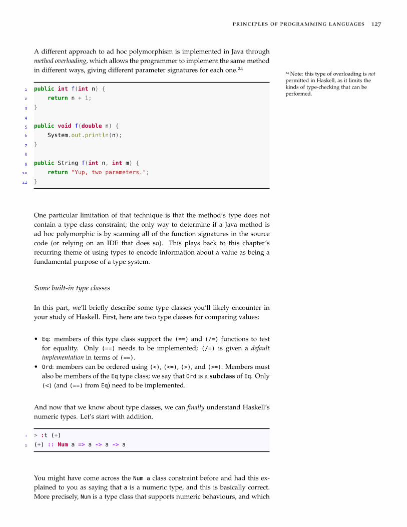
principles of programming languages 127
A different approach to ad hoc polymorphism is implemented in Java throughmethod overloading, which allows the programmer to implement the same methodin different ways, giving different parameter signatures for each one.24
24 Note: this type of overloading is notpermitted in Haskell, as it limits thekinds of type-checking that can beperformed.
1 public int f(int n) {
2 return n + 1;
3 }
4
5 public void f(double n) {
6 System.out.println(n);
7 }
8
9 public String f(int n, int m) {
10 return "Yup, two parameters.";
11 }
One particular limitation of that technique is that the method’s type does notcontain a type class constraint; the only way to determine if a Java method isad hoc polymorphic is by scanning all of the function signatures in the sourcecode (or relying on an IDE that does so). This plays back to this chapter’srecurring theme of using types to encode information about a value as being afundamental purpose of a type system.
Some built-in type classes
In this part, we’ll briefly describe some type classes you’ll likely encounter inyour study of Haskell. First, here are two type classes for comparing values:
• Eq: members of this type class support the (==) and (/=) functions to testfor equality. Only (==) needs to be implemented; (/=) is given a defaultimplementation in terms of (==).
• Ord: members can be ordered using (<), (<=), (>), and (>=). Members mustalso be members of the Eq type class; we say that Ord is a subclass of Eq. Only(<) (and (==) from Eq) need to be implemented.
And now that we know about type classes, we can finally understand Haskell’snumeric types. Let’s start with addition.
1 > :t (+)
2 (+) :: Num a => a -> a -> a
You might have come across the Num a class constraint before and had this ex-plained to you as saying that a is a numeric type, and this is basically correct.More precisely, Num is a type class that supports numeric behaviours, and which

128 david liu
concrete types like Integer and Float belong to. There are three main numerictype classes in Haskell:
• Num provides basic arithmetic operations such as (+), (-), and (*). Notably,it doesn’t provide a division function, as this is handled differently by itssubclasses. It also provides the function fromInteger, which we’ll discuss abit further below.
• Integral represents integers, and provides the div (integer division) and mod
functions.
1 > div 15 2
2 7
3 > :t div
4 div :: Integral a => a -> a -> a
• Fractional represents non-integral numbers, and provides the standard di-vision operator (/), among others.
So that’s it for the numeric functions. It turns out that numeric literals are alsoimpacted by type classes, which is a pretty idiosyncratic characteristic of Haskell.Let’s inspect the type of the literal 1:
1 > :t 1
2 1 :: Num a => a
Huh, it’s not Integer? That’s right, 1 (and all other integer literals) is a polymor-phic value, like []: 1 can take on any numeric type, depending on its context.This is the purpose of the fromInteger :: Num a => Integer -> a function inthe Num type class, which is called implicitly to convert integer literals into what-ever numeric type is necessary for the surrounding context.25
25 The Fractional type class has ananalogous function, fromRational, thathandles the conversion from fractionalliterals to fractional types.
By the way, this should explain why the expression 1 + 2.3 correctly returns3.3 in Haskell, even though we previously said Haskell does not have any typecoercion. When Haskell attempts to infer the type of this expression, it doesn’tautomatically assume 1 is an Integer nor 2.3 a Float. Instead, it sees that thetype of 1 must be a member of the Num type class, and the type of 2.3 must bea member of the Fractional type class, and that these two types must be equalbecause (+) takes two arguments of the same type. The Haskell compiler cancorrectly instantiate the types to satisfy these constraints, and so the type checkpasses.
Higher-order type classes
Let’s now look at one impressive feature of Haskell’s type class implementation,which goes beyond what you see in most other languages. Consider the fol-lowing problem: in addition to lists, Haskell has many other “container” types,

principles of programming languages 129
including sets and vectors. One of the particularly useful higher-order transfor-mations we have seen before is map, which is used to apply some function toeach element in a list, producing a new list as a result:
1 map :: (a -> b) -> [a] -> [b]
While this works for lists, we want such a function for sets and vectors as well:
1 setMap :: (a -> b) -> Set a -> Set b
2 vectorMap :: (a -> b) -> Vector a -> Vector b
In Racket, this is achieved by simply implementing different “mapping” func-tions for each data type, avoiding name collisions by prefixing by the data typename, just as we illustrated above. But this approach has the limitation thatwe cannot write elegant code that is polymorphic over a container type. Forexample, consider defining a function that “maps” an “add 1” function over acollection of elements, that should work regardless of the container type. InRacket, we would do something like the following:
1 (define (add1 x) (+ x 1))
2
3 (define (add-1-all items)
4 (cond
5 [(list? items) (map add1 items)]
6 [(set? items) (set-map add1 items)]
7 [(vector? items) (vector-map add1 items)]))
As you are probably thinking, the solution in Haskell seems pretty straightfor-ward: why don’t we make map part of a type class, so that we can implement itseparately for each container type? And this is indeed what Haskell does, butthere is one subtlety: since this type class would represent “container” types,its members are type constructors, not types themselves. Let’s take a look at thedefinition of the built-in “mappable” type class, which Haskell calls Functor:26
26 Many of the higher-order type classeshave names derived from an abstractbranch of mathematics called categorytheory. This isn’t relevant for thiscourse, but you might be interestedin exploring the deep relationshipsbetween type classes and categorytheory on your own time.
1 class Functor f where
2 -- the "f" in fmap stands for "Functor"
3 fmap :: (a -> b) -> f a -> f b
The type variable f represents the member of Functor, but we can tell from thetype signature of fmap that f is not a primitive type like Int or Bool, but insteada type constructor like the list ([]), Set, or Vector. And because Haskell makesthese different data types instances of Functor, we can implement a “map plus1” function to work on arbitrary containers:

130 david liu
1 add1All :: Functor f => f Int -> f Int
2 add1All items = fmap (+1) items
3
4 -- Or, using currying:
5 add1All = fmap (+1)
Representing failing computations
Here’s an interesting type that really illustrates the purpose of having multipledata constructors. Suppose you have an initial value, and want to perform aseries of computations on this value, but each computation has a chance offailing. We would probably handle this in other programming languages byusing exceptions or by checking each step to see if the returned value indicatesan error. Both of these strategies often introduce extra runtime risk into ourprogram, because the compiler cannot always determine whether (or what kindof) an exception will be raised,27 or distinguish between valid and erroneous
27 Though this is mitigated in Java withchecked exceptions.return values, leaving it to the programmer to remember to make the check.
Lest we get too high on our Haskell horse, be reminded that we have seen unsafefunctions in Haskell as well: head, tail, and any incomplete pattern matches,for example. In this section, we will see how to incorporate this possibility oferror in a statically-checkable way, using Haskell’s type system. That is, we canindicate in our programs where potentially failing computations might occur,and make this known to the compiler by defining a data type representing theresult of a computation that may or may not have been successful.
We start by introducing the fundamental type constructor, Maybe, used to repre-sent such values.28
28 Java 8 introduced the analogousOptional type.
1 data Maybe a = Nothing | Just a
Intuitively, the type Maybe a represents values that could have two possiblestates: either they’re a Nothing, because they were produced by some com-putation that failed, or they’re an actual a value, because the computation suc-ceeded. Many programming languages encode this idea implicitly through aspecial value like None or null or nil; Haskell goes a step further, using notjust an analogous value Nothing, but also encoding this in the very type of theexpression: Maybe Int is not the same as Int, and the compiler can tell the dif-ference!
Here are some simple functions that illustrate this data type; note that the“wrapped” type a can be anything, as Maybe is a generic type.
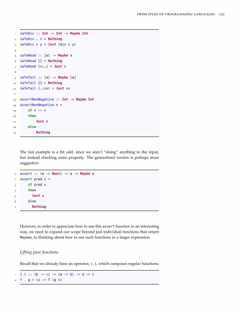
principles of programming languages 131
1 safeDiv :: Int -> Int -> Maybe Int
2 safeDiv _ 0 = Nothing
3 safeDiv x y = Just (div x y)
4
5 safeHead :: [a] -> Maybe a
6 safeHead [] = Nothing
7 safeHead (x:_) = Just x
8
9 safeTail :: [a] -> Maybe [a]
10 safeTail [] = Nothing
11 safeTail (_:xs) = Just xs
12
13 assertNonNegative :: Int -> Maybe Int
14 assertNonNegative n =
15 if n >= 0
16 then
17 Just n
18 else
19 Nothing
The last example is a bit odd, since we aren’t “doing” anything to the input,but instead checking some property. The generalized version is perhaps moresuggestive:
1 assert :: (a -> Bool) -> a -> Maybe a
2 assert pred x =
3 if pred x
4 then
5 Just x
6 else
7 Nothing
However, in order to appreciate how to use this assert function in an interestingway, we need to expand our scope beyond just individual functions that returnMaybes, to thinking about how to use such functions in a larger expression.
Lifting pure functions
Recall that we already have an operator, (.), which composes regular functions:
1 (.) :: (b -> c) -> (a -> b) -> a -> c
2 f . g = \x -> f (g x)

132 david liu
Let’s start with a simple example: defining a function that takes the first elementof a list of numbers, and adds 1 to that number. If we weren’t worried aboutruntime errors, we could define this function as follows:29
29 We deliberately write this in a terserstyle to emphasize the composition ofthe main functions involved. Make sureyou understand this definition beforemoving on!
1 add1ToHead :: [Int] -> Int
2 add1ToHead = (+1) . head
It is tempting to make this function “safe” by swapping in our safeHead fromabove, and returning a Maybe:
1 safeAdd1ToHead :: [Int] -> Maybe Int
2 safeAdd1ToHead = (+1) . safeHead
Unfortunately, this implementation doesn’t type-check. The problem is that (+1)expects a “pure” numeric type (like Int), but we’re giving it a Maybe Int instead.Now, we could define a new function to handle this explicitly using pattern-matching:
1 add1Maybe :: Maybe Int -> Maybe Int
2 add1Maybe Nothing = Nothing
3 add1Maybe (Just n) = Just (n + 1)
But of course this approach doesn’t scale; we don’t want to have to define “Maybeversions” of every function we want to use. Instead we define a higher-order func-tion that will take any pure a -> b function and turn it into one that works onMaybe as instead. We call this operation lift, taking the term from mathemat-ics, usually denoting the transformation of some object to move it into a moreabstract or general context.
1 lift :: (a -> b) -> (Maybe a -> Maybe b)
2 lift _ Nothing = Nothing
3 lift f (Just x) = Just (f x)
With this function, we can complete a correct implementation of safeAdd1ToHead:
1 safeAdd1ToHead :: [Int] -> Maybe Int
2 safeAdd1ToHead = (lift (+1)) . safeHead
But hang on: doesn’t the type signature for lift look a little familiar? Keepin mind that -> is right-associative in type expressions, and so that second pairaren’t necessary:

principles of programming languages 133
1 lift :: (a -> b) -> Maybe a -> Maybe b
You guessed it! This expression exactly matches the one for fmap, and this isn’ta coincidence: Maybe is indeed a member of the Functor type class.30
30 Indeed, we can think about Maybe asa “container” that holds exactly zero orone value of its contained type.1 safeAdd1ToHead :: [Int] -> Maybe Int
2 safeAdd1ToHead = (fmap (+1)) . safeHead
Composing failing computations
Now let’s consider defining a function that returns the second element of a list:
1 second :: [a] -> a
2 second = head . tail
Our first attempt at making this function safe is to replace the list functions withthe safe variants we defined above:
1 safeSecond :: [a] -> Maybe a
2 safeSecond = safeHead . safeTail
It looks like we have a similar problem as before: safeTail returns a Maybe [a],while safeHead expects just a [a]. What happens if we try using fmap (or lift)?
1 safeSecond :: [a] -> Maybe a
2 safeSecond = (fmap safeHead) . safeTail
Unfortunately, this doesn’t quite work: the return type is a Maybe (Maybe a),rather than just a Maybe a! This isn’t what we want, so we’re going to take adifferent (presumably also higher-order) approach. But what? Let’s start bywriting a correct, if cumbersome, implementation of safeSecond.31
31 This also introduces case expressions,which enable pattern-matching inarbitrary expression contexts.1 safeSecond :: [a] -> Maybe a
2 safeSecond xs =
3 let xs' = safeTail xs
4 in
5 case xs' of
6 Nothing -> Nothing
7 Just xs'' -> safeHead xs''

134 david liu
To see what’s going on, let’s inspect the types:
• xs has type [a], which is the original input to the function• xs' has type Maybe [a], which is what’s returned by safeTail
• xs'' has type [a]: it is an “unwrapped” version of xs', which is safe to doinside the case expression because we provide pattern-match rules for bothpossibilities for xs'.
Unfortunately, using the case expression does not generalize very elegantly, aswe compose more and more computations. Suppose we wanted to access thefourth element of a list:
1 safeFourth :: [a] -> Maybe a
2 safeFourth xs =
3 let xs' = safeTail xs
4 in
5 case xs' of
6 Nothing -> Nothing
7 Just xs1 ->
8 let xs1' = safeTail xs1
9 in
10 case xs1' of
11 Nothing -> Nothing
12 Just xs2 ->
13 let xs2' = safeTail xs2
14 case xs2' of
15 Nothing -> Nothing
16 Just xs3 -> safeHead xs3
To remove the code duplication, we move the pattern-matching to a helper:32
32 The name andThen should suggest theidea of sequencing multiple computa-tions.1 andThen :: Maybe a -> (a -> Maybe b) -> Maybe b
2 andThen Nothing _ = Nothing
3 andThen (Just x) f = f x
Like lift, the implementation of andThen is very simple. The only differenceis that we do not wrap the second line’s body in a Just (logically, we shouldn’tassume that calling f will succeed!). Let’s use this helper to see how to simplifysafeSecond:
1 safeSecond :: [a] -> Maybe a
2 safeSecond xs =
3 let xs' = safeTail xs
4 in
5 andThen xs' safeHead

principles of programming languages 135
However, this isn’t that readable. The reason we chose the name andThen onlybecomes apparent when we use backticks to call andThen from an infix position:
1 safeSecond :: [a] -> Maybe a
2 safeSecond xs =
3 let xs' = safeTail xs
4 in
5 xs' `andThen` safeHead
6
7 -- Or simply,
8 safeSecond xs = safeTail xs `andThen` safeHead
With this use of andThen, we can entirely remove all of the boilerplate fromsafeFourth as well, resulting in a truly beautiful implementation.
1 safeFourth :: [a] -> Maybe a
2 safeFourth xs =
3 safeTail xs `andThen`
4 safeTail `andThen`
5 safeTail `andThen`
6 safeHead
Error reporting
One limitation of using Maybe is that chained computations don’t preserve in-formation about where or why the computation failed. A Nothing conveys afailure, but nothing else. In practice, the Either type constructor is often usedinstead:
1 data Either a b = Left a | Right b
Either is a versatile type constructor that can be used to represent an alterna-tive between two different types (e.g., “this function returns either an Int or aString”), but one of its most common uses is to use the Left constructor to rep-resent a failure with some error information, and a Right to represent a success,analogous to Just. For example, a bare-bones approach might store an errormessage as a string:
1 safeDiv2 :: Int -> Int -> Either String Int
2 safeDiv2 _ 0 = Left "Division by 0 error"
3 safeDiv2 x y = Right (x `div` y)
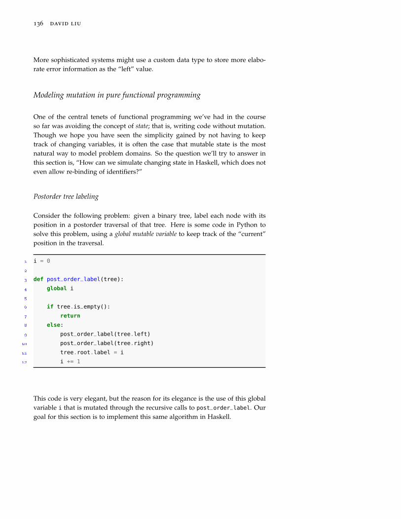
136 david liu
More sophisticated systems might use a custom data type to store more elabo-rate error information as the “left” value.
Modeling mutation in pure functional programming
One of the central tenets of functional programming we’ve had in the courseso far was avoiding the concept of state; that is, writing code without mutation.Though we hope you have seen the simplicity gained by not having to keeptrack of changing variables, it is often the case that mutable state is the mostnatural way to model problem domains. So the question we’ll try to answer inthis section is, “How can we simulate changing state in Haskell, which does noteven allow re-binding of identifiers?”
Postorder tree labeling
Consider the following problem: given a binary tree, label each node with itsposition in a postorder traversal of that tree. Here is some code in Python tosolve this problem, using a global mutable variable to keep track of the “current”position in the traversal.
1 i = 0
2
3 def post_order_label(tree):
4 global i
5
6 if tree.is_empty():
7 return
8 else:
9 post_order_label(tree.left)
10 post_order_label(tree.right)
11 tree.root.label = i
12 i += 1
This code is very elegant, but the reason for its elegance is the use of this globalvariable i that is mutated through the recursive calls to post_order_label. Ourgoal for this section is to implement this same algorithm in Haskell.

principles of programming languages 137
Stateful computations
Believe it or not, we have already seen the basic “mutating state” technique inthis course. Recall the basic loop iteration pattern:
1 acc = init
2 for x in lst:
3 acc = update(x, acc)
We achieved the same affect using foldl, and the key idea was that the updatefunction passed to foldl was interpreted to “mutate” the accumulator. Con-cretely, the function took as input the old state of the accumulator, and returnedits new state. By chaining together such functions—each taking the result of theprevious—we can simulate a mutating “accumulated state” over many differentcomputations.
For any kind of mutable state, the two primitive operations are read and write,which here we’ll label get and put. We could implement each one as follows:
1 get :: s -> s
2 get state = state
3
4 put :: s -> s -> s
5 put item state = item
This looks a bit strange, so let’s unpack our intentions. - get takes in the currentstate and simply returns it; this simulates “reading” from the state. - put takes anitem and the current state, and returns the item, representing the new state (notethat the old state is completely discarded). Right now, it is impossible to tellfrom the return types of these two functions that one of them returns a lookupvalue (but leaves the state unchanged), and the other actually modifies the storedstate. To resolve this issue, we unify their return types by using a tuple, wherethe first element of the tuple represents what value (if any) is “produced” by thecomputation, and the second element represents the new state.
1 get :: s -> (s, s)
2 get state = (state, state)
3
4 put :: s -> s -> ((), s)
5 put item state = ((), item)
Now let’s interpret this new code: - get takes the old state and returns its valueas both elements of the tuple. The first element represents what’s being pro-duced (the value is looked up), while the second represents the new state, whichis actually exactly the same as the old state. - put updates the state, which is

138 david liu
why the second element in the returned tuple is item—the old state has beenreplaced. The () in the first position is called unit in Haskell,33 and is used to
33 Somewhat confusingly, () is both avalue and a type, both called “unit”.denote the fact that the put doesn’t produce a value. This is analogous to a void
return type in Java or C.
That’s better, but we’ll go one step further and use Haskell’s built-in State datatype, which essentially wraps around the “updating state” function type:
1 data State s a = State (s -> (a, s))
2
3 get :: State s s
4 get = State (\state -> (state, state))
5
6 put :: s -> State s ()
7 put item = State (\state -> ((), item))
Warning: State is actually a pretty confusing name. In Haskell, this State typeconstructor doesn’t refer to the state itself, but rather to a stateful computation thattakes in and returns state, as we described above. This is a pretty unfortunatehistorical name, so please pay attention to the name when we use it through thissection!
So using this language, we say that get is a stateful computation that produceswhat was stored in the state and leaves the state unchanged, while put is astateful computation that takes an item, and replaces the existing state with thatitem, but doesn’t produce a value.
Running and combining stateful computations
One of the side effects of using the State type to represent stateful computationsis that the underlying function is now wrapped, and can’t be called directly. Forexample, calling get 5 produces an error rather than the expected (5, 5). Toresolve this, Haskell has a built-in function runState whose only purpose is toreturn the wrapped function:
1 runState :: State s a -> (s -> (a, s))
2 runState (State op) = op
But in the above code, op is a function; in order to actually “execute” the statefulcomputation, we need to pass in a state value, which we think of as representingthe initial state.
1 > runState get 5
2 (5,5)
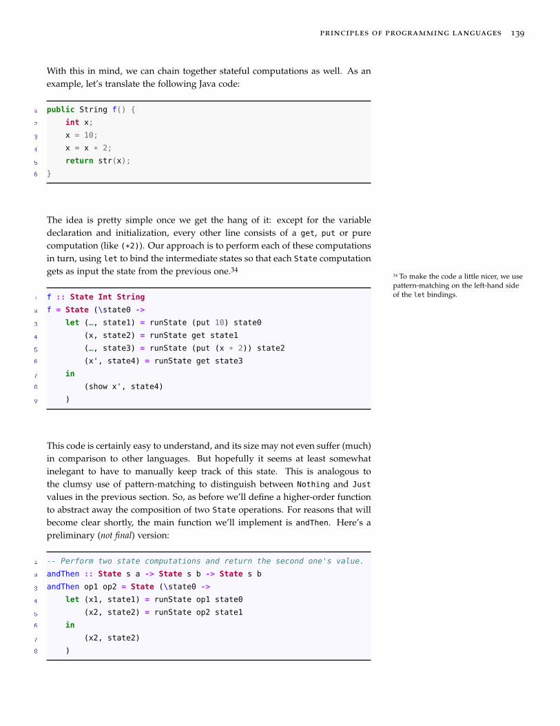
principles of programming languages 139
With this in mind, we can chain together stateful computations as well. As anexample, let’s translate the following Java code:
1 public String f() {
2 int x;
3 x = 10;
4 x = x * 2;
5 return str(x);
6 }
The idea is pretty simple once we get the hang of it: except for the variabledeclaration and initialization, every other line consists of a get, put or purecomputation (like (*2)). Our approach is to perform each of these computationsin turn, using let to bind the intermediate states so that each State computationgets as input the state from the previous one.34
34 To make the code a little nicer, we usepattern-matching on the left-hand sideof the let bindings.1 f :: State Int String
2 f = State (\state0 ->
3 let (_, state1) = runState (put 10) state0
4 (x, state2) = runState get state1
5 (_, state3) = runState (put (x * 2)) state2
6 (x', state4) = runState get state3
7 in
8 (show x', state4)
9 )
This code is certainly easy to understand, and its size may not even suffer (much)in comparison to other languages. But hopefully it seems at least somewhatinelegant to have to manually keep track of this state. This is analogous tothe clumsy use of pattern-matching to distinguish between Nothing and Just
values in the previous section. So, as before we’ll define a higher-order functionto abstract away the composition of two State operations. For reasons that willbecome clear shortly, the main function we’ll implement is andThen. Here’s apreliminary (not final) version:
1 -- Perform two state computations and return the second one's value.
2 andThen :: State s a -> State s b -> State s b
3 andThen op1 op2 = State (\state0 ->
4 let (x1, state1) = runState op1 state0
5 (x2, state2) = runState op2 state1
6 in
7 (x2, state2)
8 )
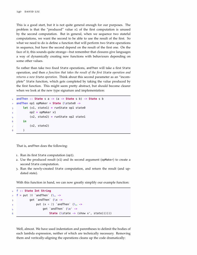
140 david liu
This is a good start, but it is not quite general enough for our purposes. Theproblem is that the “produced” value x1 of the first computation is unusedby the second computation. But in general, when we sequence two statefulcomputations, we want the second to be able to use the result of the first. Sowhat we need to do is define a function that will perform two State operationsin sequence, but have the second depend on the result of the first one. On theface of it, this sounds quite strange—but remember that closures give languagesa way of dynamically creating new functions with behaviours depending onsome other values.
So rather than take two fixed State operations, andThen will take a first Stateoperation, and then a function that takes the result of the first State operation andreturns a new State operation. Think about this second parameter as an “incom-plete” State function, which gets completed by taking the value produced bythe first function. This might seem pretty abstract, but should become clearerwhen we look at the new type signature and implementation:
1 andThen :: State s a -> (a -> State s b) -> State s b
2 andThen op1 opMaker = State (\state0 ->
3 let (x1, state1) = runState op1 state0
4 op2 = opMaker x1
5 (x2, state2) = runState op2 state1
6 in
7 (x2, state2)
8 )
That is, andThen does the following:
1. Run its first State computation (op1).2. Use the produced result (x1) and its second argument (opMaker) to create a
second State computation.3. Run the newly-created State computation, and return the result (and up-
dated state).
With this function in hand, we can now greatly simplify our example function:
1 f :: State Int String
2 f = put 10 `andThen` (\_ ->
3 get `andThen` (\x ->
4 put (x + 2) `andThen` (\_ ->
5 get `andThen` (\x' ->
6 State (\state -> (show x', state))))))
Well, almost. We have used indentation and parentheses to delimit the bodies ofeach lambda expression, neither of which are technically necessary. Removingthem and veritcally-aligning the operations cleans up the code dramatically:

principles of programming languages 141
1 f :: State Int String
2 f = put 10 `andThen` \_ ->
3 get `andThen` \x ->
4 put (x + 2) `andThen` \_ ->
5 get `andThen` \x' ->
6 State (\state -> (show x', state))
Finally, we note that the final State value is special, since it simply “produces”a value (show x') without any interaction with the underlying state at all. We’llcall this type of computation a “pure” one, and use a helper function to simplifythe code further:
1 pureValue :: a -> State s a
2 pureValue item = State (\state -> (item, state))
3
4 f :: State Int String
5 f = put 10 `andThen` \_ ->
6 get `andThen` \x ->
7 put (x + 2) `andThen` \_ ->
8 get `andThen` \x' ->
9 pureValue (show x')
Back to post-order labeling
It turns out that we have everything we need to implement a post-order binarytree labeling in Haskell. First, recall the mutating Python version:
1 i = 0
2
3 def post_order_label(tree):
4 global i
5
6 if tree.is_empty():
7 return
8 else:
9 post_order_label(tree.left)
10 post_order_label(tree.right)
11 tree.root.label = i
12 i += 1
Here is the corresponding data type we’ll use to represent binary trees in Haskell.35
35 Note the similarity to our recursivelist definition!

142 david liu
1 data BTree a = Empty
2 | Node a (BTree a) (BTree a)
To keep things immutable, we won’t mutate a BTree directly, but rather return anew BTree with all nodes labelled properly. To accomplish this using the samealgorithm as shown in the Python code, we’ll need one Int of mutable state, andso our type signature will be:36
36 In the returned tree, each node storesits original value paired with its post-order label.
1 postOrderLabel :: BTree a -> State Int (BTree (a, Int))
The base case is pretty easy to implement, and can be done without any state-fulness at all:
1 postOrderLabel Empty = pureValue Empty
As a first pass for the recursive step, let’s just try translating the two recursivecalls in Python into the equivalent chained Haskell code, using our andThen.37
37 Note that we ignore the original nodelabel, since the goal here is to set thelabel ourselves.
1 postOrderLabel (Node item left right) =
2 postOrderLabel left `andThen` \newLeft ->
3 postOrderLabel right
Not too bad, although these two recursive calls aren’t really doing anything(other than spawning other useless calls). Let’s first increment our “i”:
1 postOrderLabel (Node item left right) =
2 postOrderLabel left `andThen` \newLeft ->
3 postOrderLabel right `andThen` \newRight ->
4 get `andThen` \i ->
5 put (i + 1)
That version almost compiles, but unfortunately ends with a State value of thewrong type: State Int () instead of State Int (BTree (a, Int)). To fix this,let’s actually consider what we want to return: a new BTree with all the nodeslabeled correctly. Through the power of recursion, we can assume that bothnewLeft and newRight (produced by the recursive calls) are indeed correctlylabeled. So then to put everything together, we need to create and return a newroot node, containing the original item, an updated label, and new subtrees:

principles of programming languages 143
1 postOrderLabel (Node item left right) =
2 postOrderLabel left `andThen` \newLeft ->
3 postOrderLabel right `andThen` \newRight ->
4 get `andThen` \i ->
5 put (i + 1) `andThen` \_ ->
6 pureValue (Node (item, i) newLeft newRight)
And that’s it! Not too shabby indeed—and quite close to what we’d write inPython if we had to return a new tree rather than mutate the original.
Impure I/O in a pure functional world
In addition to mutating state, another common type of impure function is onethat interacts with some entity external to the program:38 standard input or
38 Functions receiving external inputare impure because their behaviourchanges each time they are run; func-tions writing to some output are im-pure because they have a side-effect.
output, a graphical display, the filesystem, or a server thousands of kilometresaway. Even though we’ve been programming without explicit mention of I/Osince the beginning of the term, it’s always been present: any REPL requiresfunctions that take in user input, and that actually display the output to the useras well. If Haskell had no I/O capabilities whatsoever, we would never know ifa program actually worked or not, since we would have no way to observe itsoutput!
In this section, we’ll briefly study how Haskell programs can interact directlywith the standard input and standard output provided by the operating system.While the primitives we’ll use in this section might look underwhelming, all ofthe other I/O operations we mentioned above behave exactly the same. In fact,even more is true: it turns out that all I/O follows our approach to mutable statefrom the previous section. Even though both I/O and mutation are side-effectfulbehaviours, they seem quite different at first glance, and so this might come asa surprise. Let’s take a closer look at what’s going on.
Our State s a values represented computations with two behaviours: a “pure”part, the computation performed to produce a value, and an impure part, a“mutation” operation, representing an interaction with the underlying context ofthe computation. We can think of pure functions as those that have no context(e.g., external mutable state) they need to reference, and impure functions asthose that do.
Even though our post-order labeling example used a State Int representing justone integer’s worth of mutable state, the beauty of the State type constructoris that it can be parameterized on the type of state s being used, and so inmore complex programs we might have State String or State [Int] or evenState (Map String Expr).39 But even this view is too narrow: there is no need
39 Think back to our previous discus-sions of the environment. . .to limit our computational context to the program’s heap-allocated memory. By
widening the scope of this context to user interactions, files, and faraway servers,we can model any type of I/O computation at all.
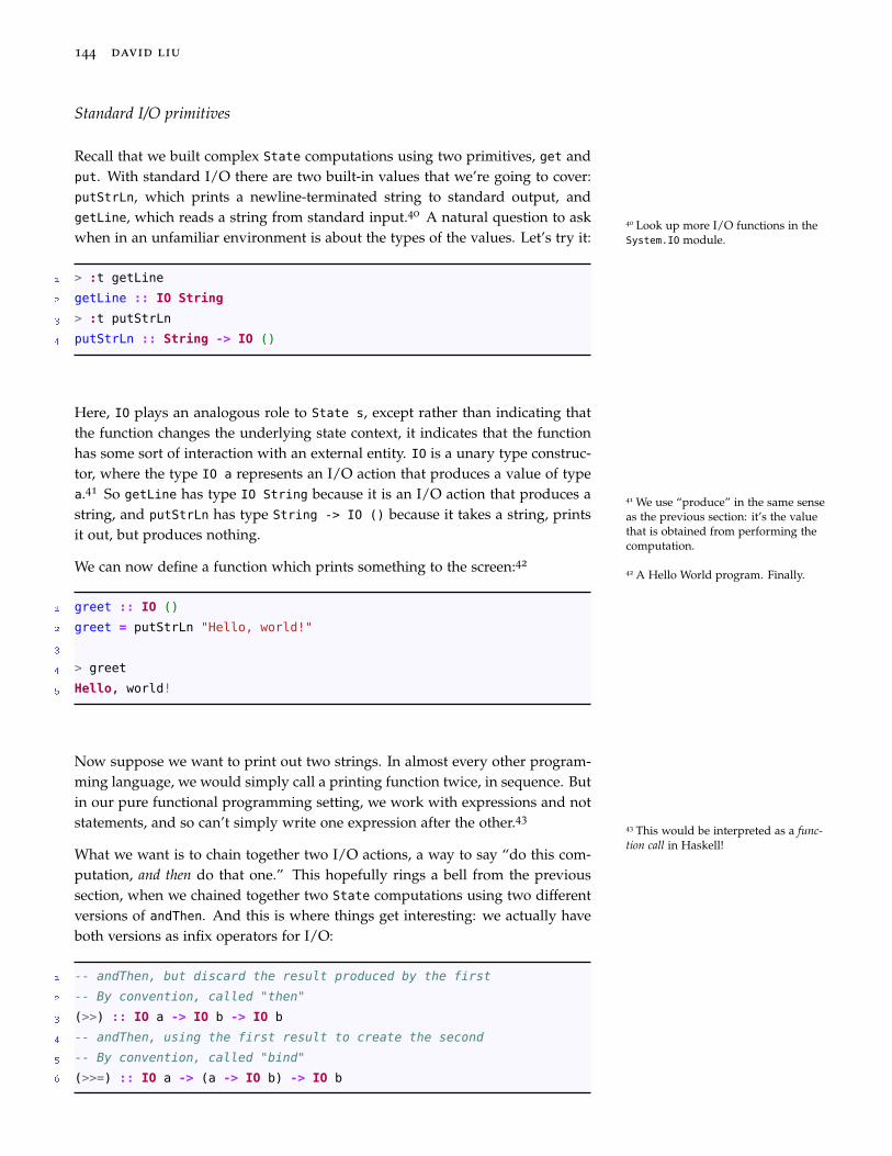
144 david liu
Standard I/O primitives
Recall that we built complex State computations using two primitives, get andput. With standard I/O there are two built-in values that we’re going to cover:putStrLn, which prints a newline-terminated string to standard output, andgetLine, which reads a string from standard input.40 A natural question to ask
40 Look up more I/O functions in theSystem.IO module.when in an unfamiliar environment is about the types of the values. Let’s try it:
1 > :t getLine
2 getLine :: IO String
3 > :t putStrLn
4 putStrLn :: String -> IO ()
Here, IO plays an analogous role to State s, except rather than indicating thatthe function changes the underlying state context, it indicates that the functionhas some sort of interaction with an external entity. IO is a unary type construc-tor, where the type IO a represents an I/O action that produces a value of typea.41 So getLine has type IO String because it is an I/O action that produces a
41 We use “produce” in the same senseas the previous section: it’s the valuethat is obtained from performing thecomputation.
string, and putStrLn has type String -> IO () because it takes a string, printsit out, but produces nothing.
We can now define a function which prints something to the screen:42
42 A Hello World program. Finally.
1 greet :: IO ()
2 greet = putStrLn "Hello, world!"
3
4 > greet
5 Hello, world!
Now suppose we want to print out two strings. In almost every other program-ming language, we would simply call a printing function twice, in sequence. Butin our pure functional programming setting, we work with expressions and notstatements, and so can’t simply write one expression after the other.43
43 This would be interpreted as a func-tion call in Haskell!
What we want is to chain together two I/O actions, a way to say “do this com-putation, and then do that one.” This hopefully rings a bell from the previoussection, when we chained together two State computations using two differentversions of andThen. And this is where things get interesting: we actually haveboth versions as infix operators for I/O:
1 -- andThen, but discard the result produced by the first
2 -- By convention, called "then"
3 (>>) :: IO a -> IO b -> IO b
4 -- andThen, using the first result to create the second
5 -- By convention, called "bind"
6 (>>=) :: IO a -> (a -> IO b) -> IO b

principles of programming languages 145
It shouldn’t be a big surprise that we can use the former to sequence two ormore I/O actions:
1 greet2 :: IO ()
2 greet2 =
3 putStrLn "Hello, world!" >>
4 putStrLn "Second line time!"
5
6 prompt :: IO ()
7 prompt =
8 putStrLn "What's your name?" >>
9 getLine >>
10 putStrLn "Nice to meet you, ____!"
How do we fill in the blank? We need to take the string produced by the getLine
and use it to define the next I/O action. Again, this should be ringing lots ofbells, because this is exactly what we did with our final version of andThen,corresponding to the I/O operator (>>=):
1 prompt2 :: IO ()
2 prompt2 =
3 putStrLn "What's your name?" >>
4 getLine >>= \name ->
5 putStrLn "Nice to meet you, " ++ name ++ "!"
6
7 > prompt2
8 What's your name?
9 David -- This line is user input
10 Nice to meet you, David!
Standalone Haskell programs
Though we’ve mainly used GHCi, Haskell programs can also be compiled andrun.44 Such programs require a main function with type IO (), which is executed
44 Say, by using the commandrunhaskell myfile.hs.when the program is run. The type of main is very suggestive: the program as
a whole is an IO action that can interact with the outside world, using main asits entry point. In this course we’ve been mainly using the REPL as our entrypoint, but in practice any kind of I/O behaviour would start under main.
Types as constraints
You have now seen two examples of impure values in Haskell: the state-“mutating”State computations, and the external-world-interacting IO. Despite our prior

146 david liu
insistence that functional programming is truly different, it seems possible tosimulate imperative programs using these functions and others like them. Thisis technically correct, but it misses a very important point: unlike other lan-guages, Haskell’s type system enforces a strict separation between pure andimpure code.
The separation of concerns principle is one of the most well-known in computerscience, and you’ve probably studied this extensively in the context of design-ing classes, libraries, and larger application architectures like MVC. However,in most languages, is easy for impure and pure code to be tightly wound to-gether, because side-effecting behaviour like mutation and I/O is taught to usfrom our very beginnings as programmers. But as we’ve discussed earlier, thiscoupling makes programs difficult to reason about, and often in our refactoringwe expend great effort understanding and simplifying such side-effects.
In stark contrast, such mixing is explicitly forbidden by Haskell’s type system.Think back to IO. We only used functions that combine values of IO types (like(>>=)), or functions that returned a value of these types. But once the IO wasintroduced, there was no way to get rid of it: there is no function IO a -> a.45
45 This isn’t strictly true, but the func-tions that do exist are used rarely andwith great care in Haskell production.
This means that any Haskell function that uses standard I/O must have a IO in itstype.
It might feel restrictive to say that every time you want to print something in afunction, you must change the fundamental type (and hence structure) of thatfunction. However, as a corollary of this, any function that doesn’t have IO inits type is guaranteed not to interact with the terminal, and this guarantee isprovided at compile time, just through the use of types! This is perhaps the bestillustration of this chapter’s central principle: a type signature in Haskell tellsus not just how to use a function and what it returns, but what it cannot do aswell.
One last abstraction: monads
When we first started our study of types and Haskell, you might have thoughtwe would focus on the syntax of creating new types in Haskell. But even thoughwe did introduce quite a few new keywords for Haskell’s type system, our am-bitions were far grander than recreating a classical object-oriented system inHaskell.46 Rather than focusing on types representing concrete models or actors
46 We (basically) already did this inRacket.in our programs, we have focused on using types to encode generic modes of
computation: failing computations, stateful computations, and I/O computa-tions.
But defining type constructors like Maybe, State, and IO to represent elementsof these computations was only a small part of what we did. After definingMaybe and State, we could have performed any computation we wanted to withthese types simply by using let bindings, and called it a day. The novel partwas really our use of higher-order functions to abstract away even how we com-puted on these types, allowing us to elegantly compose primitive values of thesetypes to express complex computations. And this, of course, is the true spirit of
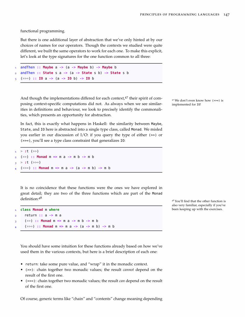
principles of programming languages 147
functional programming.
But there is one additional layer of abstraction that we’ve only hinted at by ourchoices of names for our operators. Though the contexts we studied were quitedifferent, we built the same operators to work for each one. To make this explicit,let’s look at the type signatures for the one function common to all three:
1 andThen :: Maybe a -> (a -> Maybe b) -> Maybe b
2 andThen :: State s a -> (a -> State s b) -> State s b
3 (>>=) :: IO a -> (a -> IO b) -> IO b
And though the implementations differed for each context,47 their spirit of com-47 We don’t even know how (>>=) isimplemented for IO!posing context-specific computations did not. As always when we see similar-
ities in definitions and behaviour, we look to precisely identify the commonali-ties, which presents an opportunity for abstraction.
In fact, this is exactly what happens in Haskell: the similarity between Maybe,State, and IO here is abstracted into a single type class, called Monad. We misledyou earlier in our discussion of I/O: if you query the type of either (>>) or(>>=), you’ll see a type class constraint that generalizes IO:
1 > :t (>>)
2 (>>) :: Monad m => m a -> m b -> m b
3 > :t (>>=)
4 (>>=) :: Monad m => m a -> (a -> m b) -> m b
It is no coincidence that these functions were the ones we have explored ingreat detail; they are two of the three functions which are part of the Monad
definition:48
48 You’ll find that the other function isalso very familiar, especially if you’vebeen keeping up with the exercises.1 class Monad m where
2 return :: a -> m a
3 (>>) :: Monad m => m a -> m b -> m b
4 (>>=) :: Monad m => m a -> (a -> m b) -> m b
You should have some intuition for these functions already based on how we’veused them in the various contexts, but here is a brief description of each one:
• return: take some pure value, and “wrap” it in the monadic context.• (>>): chain together two monadic values; the result cannot depend on the
result of the first one.• (>>=): chain together two monadic values; the result can depend on the result
of the first one.
Of course, generic terms like “chain” and “contents” change meaning depending
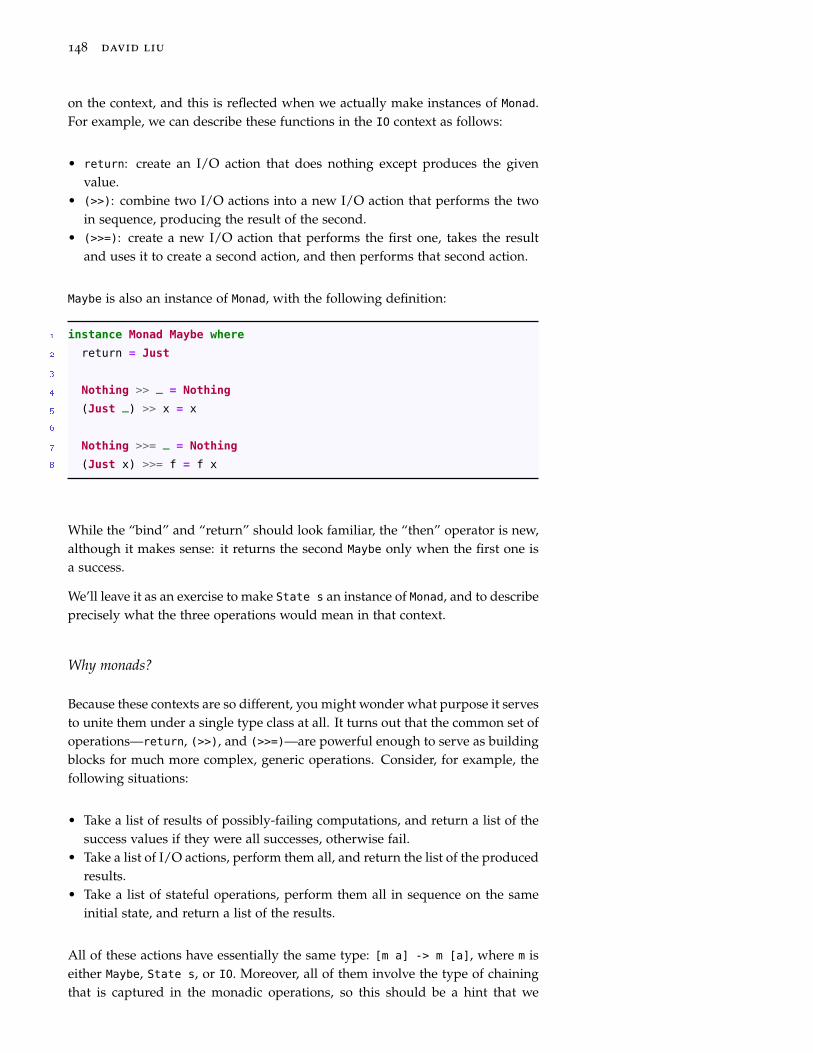
148 david liu
on the context, and this is reflected when we actually make instances of Monad.For example, we can describe these functions in the IO context as follows:
• return: create an I/O action that does nothing except produces the givenvalue.
• (>>): combine two I/O actions into a new I/O action that performs the twoin sequence, producing the result of the second.
• (>>=): create a new I/O action that performs the first one, takes the resultand uses it to create a second action, and then performs that second action.
Maybe is also an instance of Monad, with the following definition:
1 instance Monad Maybe where
2 return = Just
3
4 Nothing >> _ = Nothing
5 (Just _) >> x = x
6
7 Nothing >>= _ = Nothing
8 (Just x) >>= f = f x
While the “bind” and “return” should look familiar, the “then” operator is new,although it makes sense: it returns the second Maybe only when the first one isa success.
We’ll leave it as an exercise to make State s an instance of Monad, and to describeprecisely what the three operations would mean in that context.
Why monads?
Because these contexts are so different, you might wonder what purpose it servesto unite them under a single type class at all. It turns out that the common set ofoperations—return, (>>), and (>>=)—are powerful enough to serve as buildingblocks for much more complex, generic operations. Consider, for example, thefollowing situations:
• Take a list of results of possibly-failing computations, and return a list of thesuccess values if they were all successes, otherwise fail.
• Take a list of I/O actions, perform them all, and return the list of the producedresults.
• Take a list of stateful operations, perform them all in sequence on the sameinitial state, and return a list of the results.
All of these actions have essentially the same type: [m a] -> m [a], where m iseither Maybe, State s, or IO. Moreover, all of them involve the type of chainingthat is captured in the monadic operations, so this should be a hint that we
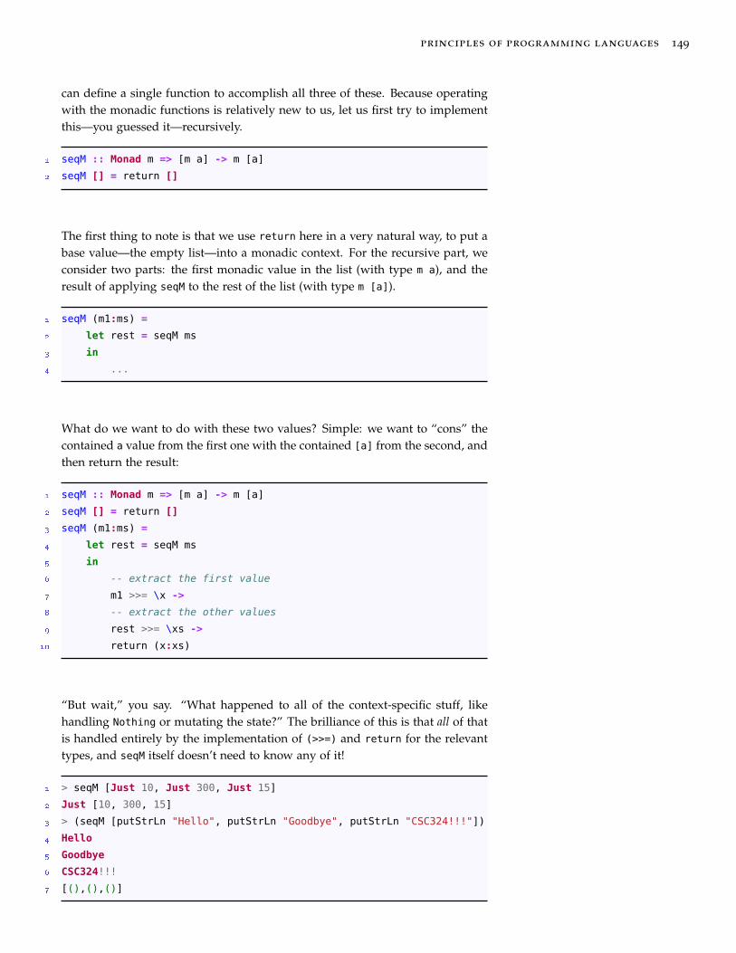
principles of programming languages 149
can define a single function to accomplish all three of these. Because operatingwith the monadic functions is relatively new to us, let us first try to implementthis—you guessed it—recursively.
1 seqM :: Monad m => [m a] -> m [a]
2 seqM [] = return []
The first thing to note is that we use return here in a very natural way, to put abase value—the empty list—into a monadic context. For the recursive part, weconsider two parts: the first monadic value in the list (with type m a), and theresult of applying seqM to the rest of the list (with type m [a]).
1 seqM (m1:ms) =
2 let rest = seqM ms
3 in
4 ...
What do we want to do with these two values? Simple: we want to “cons” thecontained a value from the first one with the contained [a] from the second, andthen return the result:
1 seqM :: Monad m => [m a] -> m [a]
2 seqM [] = return []
3 seqM (m1:ms) =
4 let rest = seqM ms
5 in
6 -- extract the first value
7 m1 >>= \x ->
8 -- extract the other values
9 rest >>= \xs ->
10 return (x:xs)
“But wait,” you say. “What happened to all of the context-specific stuff, likehandling Nothing or mutating the state?” The brilliance of this is that all of thatis handled entirely by the implementation of (>>=) and return for the relevanttypes, and seqM itself doesn’t need to know any of it!
1 > seqM [Just 10, Just 300, Just 15]
2 Just [10, 300, 15]
3 > (seqM [putStrLn "Hello", putStrLn "Goodbye", putStrLn "CSC324!!!"])
4 Hello
5 Goodbye
6 CSC324!!!
7 [(),(),()]

150 david liu
Now, this one example doesn’t mean that there aren’t times when you want,say, Maybe-specific code. Abstraction is a powerful concept, but there is a limitto how far you can abstract while still accomplishing what it is you want to do.The Monad type class is simply a tool that you can use to design far more genericcode than you probably have in other languages. But what a tool it is.
Exercise Break!
3.1 Implement seqM using foldl.
4 In Which We Say Goodbye
If all you have is a hammer,everything looks like a nail.
Law of the instrument
When teaching introductory computer science, we often deemphasize the id-iosyncrasies and minutiae of the programming language(s) we use, focusinginstead on universal theoretical and practical concepts like control flow, datastructures, modularity, and testing. Programming languages are to computerscience what screwdrivers are to carpentry: useful tools, but a means to an end.If you have a cool idea for the Next Big Thing, there are dozens, if not hundreds,of programming languages and application frameworks1 to choose from.
1 Large, monolithic frameworks areessentially specialized languagesthemselves.It is easy to get lost in the myriad technical and non-technical details that we
use to compare languages. Though these are very important—and don’t get uswrong, we covered several in this course—we must not lose sight of the forestfor the trees. At its core, the study of programming languages is the study ofhow we communicate to computers: how language constructs and features informthe properties of the code we can express.
Our first big idea was exploring how first-class functions allow us to write pro-grams in a pure functional style, achieving greater abstraction through higher-order functions and writing elegant code without side-effects. We then turned tousing macros to add two new constructs to Racket: class-based objects throughclosures, and backtracking through declarative choice expressions using contin-uations. Finally, we saw how to use a strong static type system in Haskell toencode common language features like errors, mutation, and I/O in an explicitand compile-time checkable way.
We hope you got the sense from this course that programming language researchis a truly exciting and fascinating field. If you are interested in learning more,CSC465 studies a rigorous, mathematical approach for understanding the se-mantics of (classical imperative) programming languages. CSC410 studies howto specify and ensure the correctness of programs, using a combination of staticand dynamic analysis techniques. And CSC488, our compilers course, is funda-mentally the study of translation: taking a human-readable, high-level languageand turning it into the sequence of primitive operations directly understandableby a computer.

152 david liu
Newer, modern programming languages extend the functional programmingand static analysis ideas in interesting ways. Two languages of note that drawinspiration from other domains are Elm, which uses the declarative functionalreactive programming paradigm to build web applications, and Rust, which usesstrong static analysis to add powerful compile-time safety guarantees at the lowlevel of systems programming. And of course, if you would like to talk aboutany of the material in this course or beyond, don’t be afraid to ask! That’s whatwe’re here for.