principles of roads and transport engineeringqu.edu.iq/eng/wp-content/uploads/2015/10/... ·...

Principles of Roads and Transport Engineering

1


Definitions of Transportation

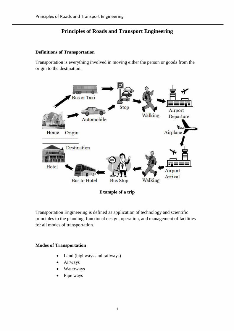
Transportation is everything involved in moving either the person or goods from the

origin to the destination.

Example of a trip

Transportation Engineering is defined as application of technology and scientific

principles to the planning, functional design, operation, and management of facilities

for all modes of transportation.

Modes of Transportation

Land (highways and railways)

Airways

Waterways

Pipe ways


2

Historical Development of Transportation

The first forms of road transport were horses, oxen or even humans

carrying goods

Wheels appear to have been developed in “ancient Sumer” in

Mesopotamia around 5000 BC

First railroad opened in 1825.

The first pipelines in the United States were introduced in 1861.

The internal-combustion engine was invented in 1866

The first electric or cable car was produced in 1880

The first diesel electric locomotive (قاطرة) was introduced in 1921

The first diesel engine buses were used in 1938

The first limited-access highway in the United States (the Pennsylvania

Turn-pike) opened in 1940

The Interstate Highway system was initiated in 1950

The first commercial jet (طائرة نفاثة) appeared in 1958

Astronauts landed on the moon in 1969

Parameters to evaluate the transportation systems

Ubiquity (االنتشار) : The amount of accessibility to the system. For example

cars are more ubiquitous than other modes of transport.

Mobility: The quantity of travel that can be handled. The capacity of a

system to handle traffic and speed are two variables connected with

mobility. A freeway has high mobility, whereas a local road has low

mobility. Water transport may have comparatively low speed, but the

capacity per vehicle is high. On the other hand, a rail system could

possibly have high speed and high capacity.

Cost

Safety

Reliability

http://en.wikipedia.org/wiki/Horse

http://en.wikipedia.org/wiki/Ox

http://en.wikipedia.org/wiki/Wheel

http://en.wikipedia.org/wiki/Sumer

http://en.wikipedia.org/wiki/Mesopotamia


3

Transportation and land use

Transportation and land use

Transportation modes choose with distance traveled

walking for short distances

car for medium distances

airplane for long distances

Transportation related problems

Fatal accidents, injuries, and property damage.

Public transportation usage is on the decline.

Transportation systems have a major impact on the environment.


4

Traffic Engineering

Traffic Engineering is defined as “a branch of engineering which applies technology,

science, and human factors to the planning, design, operations and management of

roads, streets, bikeways, highways, their networks, terminals, and abutting lands”.

Or

“The phase of transportation engineering that deals with the planning, geometric

design and traffic operations of roads, streets, and highways, their networks,

terminals, abutting lands and relationship with other modes of transportation”.

Elements of Traffic Engineering

1- Road users (drivers and pedestrians)

2- Vehicles

3- Roadway

Drivers' characteristics

1- Driving task

By keeping the vehicle at a desired speed and position with a lane, interaction

with other traffic, and reading guide signs.

2- Vision

Visual acuity

Peripheral vision

Color vision

Depth perception

Hearing perception

3- Perception-reaction time (P.I.E.V)

Perception (seeing the stimuli)

Interpretation (understanding the stimuli)

Evaluation of appropriate response (i.e., decision)

Volition or response (i.e., apply the reaction)

P.I.E.V. Refers to the time taken to detect the target, identify the target, decide

on response and initiate the response. Perception-reaction time does not

include the time to execute the decision (e.g. stop by applying a brake). The


5

perception-reaction time is not fixed for all drivers and also changes for a

same driver depend on the situations.

Factors affecting perception-reaction time

Age

Fatigue

Complexity of Cues

Presence of Drugs or Alcohol

Expectation

AASHTO (American Association of State Highways and Transportations

Officials) recommendations for reaction time:

Perception and Reaction Time: 2.5 seconds

For reaction time to traffic signal, Perception and Reaction Time: 1.0

Pedestrians' characteristics

The location of pedestrians control devices are affected by drivers as well as

pedestrian characteristics (e.g. age and speed of walking). The average walking speed

was found as about 5km/hr.

Some of pedestrians control devices

Special pedestrians’ signals

Safety zones (e.g. near the schools)


6

Pedestrians’ underpasses and elevated walkways.

Vehicles' characteristics

Vehicle types

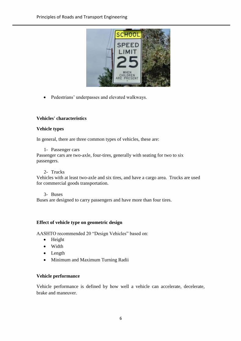
In general, there are three common types of vehicles, these are:

1- Passenger cars

Passenger cars are two-axle, four-tires, generally with seating for two to six

passengers.

2- Trucks

Vehicles with at least two-axle and six tires, and have a cargo area. Trucks are used

for commercial goods transportation.

3- Buses

Buses are designed to carry passengers and have more than four tires.

Effect of vehicle type on geometric design

AASHTO recommended 20 “Design Vehicles” based on:

Height

Width

Length

Minimum and Maximum Turning Radii

Vehicle performance

Vehicle performance is defined by how well a vehicle can accelerate, decelerate,

brake and maneuver.


7


8

Road characteristics

Factors affecting drivers’ behavior include:

Stopping sight distance

Passing sight distance

Horizontal and vertical alignments

Superelevation

Cross slope

Number of lanes

Grades

Highway classifications

Figure 1 shows an example for the highway classifications in rural area and suggests

the following types:

1- Arterial highways provide direct service between cities and larger towns (e.g.

Freeways).

2- Collector roads: serve small towns directly and connect them to the arterials.

3- Local roads: serve individual farms and other rural land uses and distribute

traffic from/to the collector roads.

Important References

Garber, N. J. and Hoel, L. A. (2009) "Traffic and Highway Engineering",

Forth Edition, Cengage learning.

Highway Capacity Manual (HCM, 2010) Transportation Research Board,

National Research Council, Washington, D.C.

A policy on Geometric Design of Highways and Streets (2004), American

Association of State Highway and Transportation Officials (AASHTO),

Washington, D.C.


9

Traffic stream elements

Traffic volume

Traffic volume is the total number of vehicles that pass over a given point or section

of a lane or roadway during a given time interval. Volumes can be expressed in terms

of veh/hr, veh/min, veh/day, …etc.

Traffic composition

Three types of vehicles are considered for the purpose of traffic analysis. These are:

Passenger cars (pcu)

Trucks and Buses

Recreational vehicles (RVs)

The overall effect of traffic operation for any vehicle type can be expressed in term of

the effect of basic unit – usually passenger car unit (pcu). Therefore, the vehicles

should be converted to pcu as follows:

Example: a rural highway on a level terrain has the following traffic composition:

50% passenger cars

30% trucks

10% buses

10% recreational vehicles

Find the total volume expressed as pcu/hr if the total volume is 5000 veh/hr.

Solution:

Volume of passenger cars= 0.5*5000=2500 veh/hr

Volume of trucks =0.3*5000=1500 veh/hr

Volume of buses=0.1*5000=500 veh/hr

Volume of recreational vehicles=0.1*5000=500 veh/hr

Total volume in pcu/hr = 2500*1 + 1500*1.5 + 500*1.5 + 500*1.2

= 2500 + 2250 + 750 + 600 = 6100 pcu


11

Flow rate (q)

Flow rate is the equivalent hourly rate at which vehicles pass over a given point or

section of a lane or roadway during a given time interval of less than 1 hr, usually

15 min.

Peak flow rates and hourly volumes produce the peak-hour factor (PHF), the ratio of

total hourly volume to the peak flow rate within the hour, computed by the following

Equation:

Example: traffic volume data has been collected for 15 min time intervals as shown

below. Find the total hourly volume, flow rate and peak hour factor (PHF).

Time 7:30 – 7:45 7:45 – 8:00 8:00 – 8:15 8:15 – 8:30

Volume 250 350 300 200

Solution:

Volume = 250+350+300+200 = 1100 veh

Flow rate (q) = peak volume * number of intervals per 1 hour

= 350 * 4 = 1400 veh/hr

PHF=1100/1400=0.786

Example: traffic volume data has been collected for 10 min time intervals as shown

below. Find the total hourly volume, flow rate and PHF.

Time 7:30–7:40 7:40–7:50 7:50–8:00 8:00–8:10 8:10–8:20 8:20–8:30

Volume 150 200 300 200 150 100

Solution:

Volume = 150+200+300+200+150+100= 1100 veh

Flow rate (q) = peak volume * number of intervals per 1 hour

= 300 * 6 = 1800 veh/hr

PHF=1100/1800=0.61


11

Speed

Speed (u) is the distance traveled by a vehicle during a unit of time. It can be

expressed in miles per hour (mi/h), kilometers per hour (km/h), or feet per second

(ft /sec).

Types of speeds

Several different speed parameters can be applied to a traffic stream. These include

the following:

Average running speed: A traffic stream measure based on the observation of

vehicle travel times traversing a section of highway of known length. It is the length

of the segment divided by the average running time of vehicles to traverse the

segment. Running time includes only time that vehicles are in motion.

Average travel speed (Journey speed): A traffic stream measure based on travel

time observed on a known length of highway. It is the length of the segment divided

by the average travel time of vehicles traversing the segment, including all stopped

delay times. It is also a space mean speed.

Space mean speed: A statistical term denoting an average speed based on the average

travel time of vehicles to traverse a segment of roadway.

where

space mean speed (km /hr)

n number of vehicles

ti the time it takes the ith vehicle to travel across a section of highway (sec)

ui speed of the ith vehicle (km /hr)

L length of section of highway (km)


12

Time mean speed (spot speed): The arithmetic average of speeds of vehicles

observed passing a point on a highway; also referred to as the average spot speed.

The individual speeds of vehicles passing a point are recorded and averaged

arithmetically.

where

t): time mean speed (km/hr)

n: number of vehicles passing a point on the highway

ui: speed of the ith vehicle (km /hr)

Free-flow speed: The average speed of vehicles on a given facility, measured under

low-volume conditions, when drivers tend to drive at their desired speed and are not

constrained by control delay.

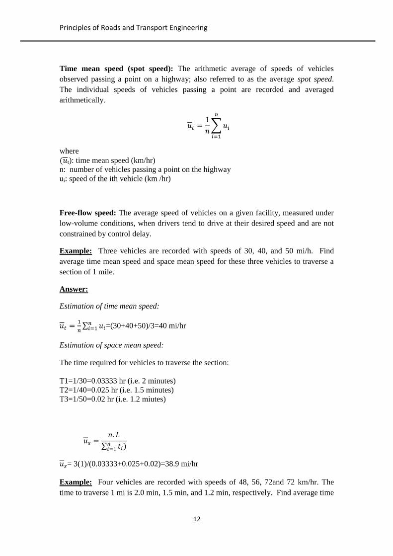
Example: Three vehicles are recorded with speeds of 30, 40, and 50 mi/h. Find

average time mean speed and space mean speed for these three vehicles to traverse a

section of 1 mile.

Answer:

Estimation of time mean speed:

=(30+40+50)/3=40 mi/hr

Estimation of space mean speed:

The time required for vehicles to traverse the section:

T1=1/30=0.03333 hr (i.e. 2 minutes)

T2=1/40=0.025 hr (i.e. 1.5 minutes)

T3=1/50=0.02 hr (i.e. 1.2 miutes)

= 3(1)/(0.03333+0.025+0.02)=38.9 mi/hr

Example: Four vehicles are recorded with speeds of 48, 56, 72and 72 km/hr. The

time to traverse 1 mi is 2.0 min, 1.5 min, and 1.2 min, respectively. Find average time


13

mean speed and space mean speed for these four vehicles to traverse a section of

91.5m.

Answer:

Estimation of time mean speed:

=(48+56+72+72)/4= 62 km/hr

Estimation of space mean speed:

The time required for vehicles to traverse the section:

T (in seconds)=

where

S is a vehicle speed in km/hr

L is the distance traveled in meters

T1=91.5/0.278*48= 6.68sec

T2=91.5/0.278*56=5.877sec

T3=91.5/0.278*72= 4.57 sec

T4=91.5/0.278*72= 4.57sec

= 4(91.5)/(6.68+5.877+4.57+4.57)=16.87 m/sec =16.87*(3600/1000)=60.73 km/hr

Density

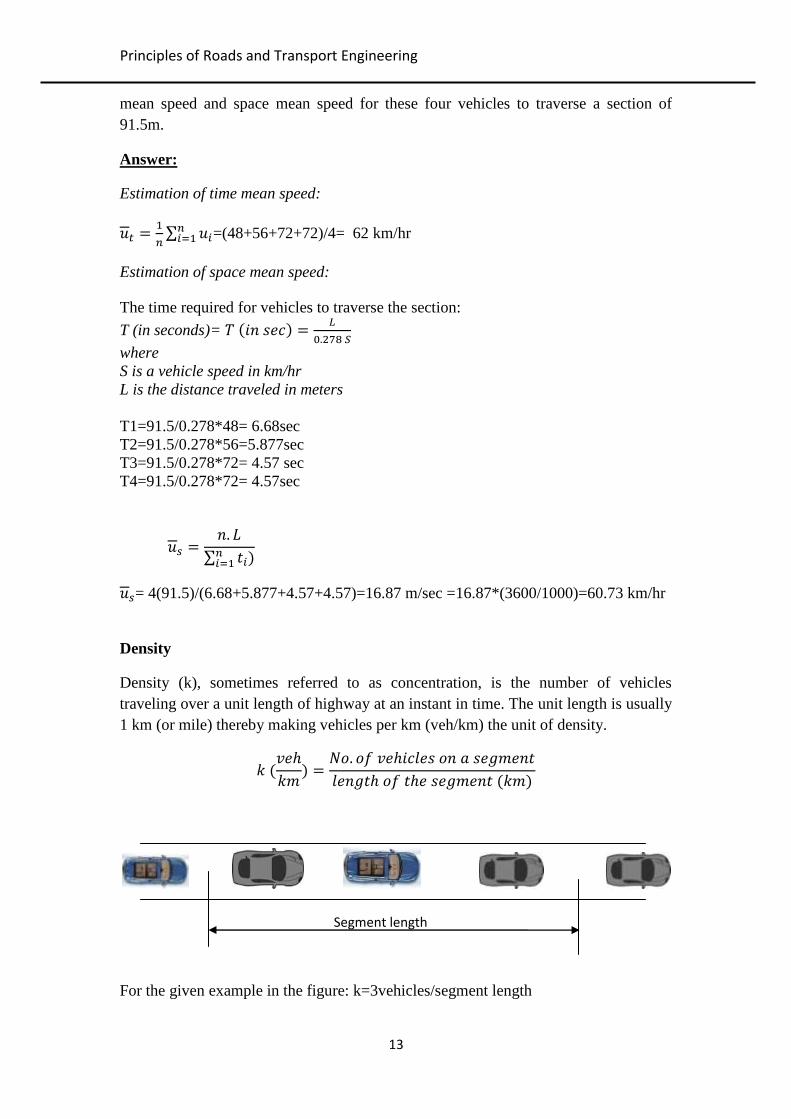
Density (k), sometimes referred to as concentration, is the number of vehicles

traveling over a unit length of highway at an instant in time. The unit length is usually

1 km (or mile) thereby making vehicles per km (veh/km) the unit of density.

For the given example in the figure: k=3vehicles/segment length

Segment length

(km)


14

Direct measurement of density in the field is difficult; therefore, density can be

computed from the average travel speed and flow rate using the following

relationship:

Where

q is the traffic flow (veh/h),

u is the average speed (space mean speed in km/h), and

k = density (veh/km).

Time Headway

Time headway (h) is the difference between the time the front of a vehicle arrives at a

point on the highway and the time the front of the next vehicle arrives at that same

point. Time headway is usually expressed in seconds.

The relationship between traffic flow and average time headway is:

Space Headway

Space headway (d) is the distance between the front of a vehicle and the front of the

following vehicle and is usually expressed in meter or feet.

Gap Headway

Gap headway is the difference in time between the time the rear of the leading vehicle

and the front of the following vehicle. Gap headway is usually expressed in seconds.

Clear spacing

Clear spacing is the difference in length between the time the rear of the leading

vehicle and the front of the following vehicle. Gap headway is usually expressed in

feet or meter.

Graph showing time headway, space headway, gap headway and clear spacing

Time headway (sec)

Space headway (m)

(sec)

Gap headway (sec)

Clear spacing (m)

Direction of traffic


15

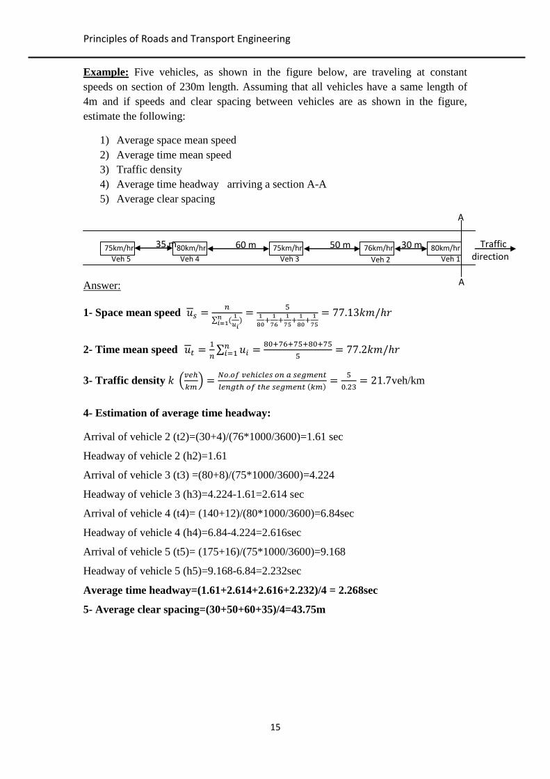
Example: Five vehicles, as shown in the figure below, are traveling at constant

speeds on section of 230m length. Assuming that all vehicles have a same length of

4m and if speeds and clear spacing between vehicles are as shown in the figure,

estimate the following:

1) Average space mean speed

2) Average time mean speed

3) Traffic density

4) Average time headway arriving a section A-A

5) Average clear spacing

Answer:

1- Space mean speed

2- Time mean speed

3- Traffic density

veh/km

4- Estimation of average time headway:

Arrival of vehicle 2 (t2)=(30+4)/(76*1000/3600)=1.61 sec

Headway of vehicle 2 (h2)=1.61

Arrival of vehicle 3 (t3) =(80+8)/(75*1000/3600)=4.224

Headway of vehicle 3 (h3)=4.224-1.61=2.614 sec

Arrival of vehicle 4 (t4)= (140+12)/(80*1000/3600)=6.84sec

Headway of vehicle 4 (h4)=6.84-4.224=2.616sec

Arrival of vehicle 5 (t5)= (175+16)/(75*1000/3600)=9.168

Headway of vehicle 5 (h5)=9.168-6.84=2.232sec

Average time headway=(1.61+2.614+2.616+2.232)/4 = 2.268sec

5- Average clear spacing=(30+50+60+35)/4=43.75m

75km/hr 80km/hr 75km/hr 76km/hr 80km/hr 30 m 50 m 60 m 35 m Traffic direction Veh 1 Veh 2 Veh 4 Veh 5 Veh 3

A

A


16

Speed-Flow-Density Diagrams

The relation between flow and density, density and speed, speed and flow, are

referred to as the fundamental diagrams of traffic flow.

a. Flow-Density curve

1. When the density is zero, flow will also be zero, since there are no vehicles on

the road.

2. When the number of vehicles gradually increases the density as well as flow

increases.

3. When more and more vehicles are added, it reaches a situation where vehicles

can’t move. This is referred to as the jam density or the maximum density. At

jam density, flow will be zero because the vehicles are not moving.

4. There will be some density between zero density and jam density, when the

flow is maximum. The relationship is normally represented by a parabolic

curve as shown in the figure.

5. The slope between point O and any other point represents the space mean

speed. For example the slope of the line OD represents the space mean speed

at density equal to k1.


17

Speed-density diagram

1. Speed will be maximum (free flow speed) , when the density is minimal

2. When the density is maximum (k=kjam), the speed will be zero.

3. The simplest assumption is that this variation of speed with density is linear as

shown by the solid line in the figure. It is also possible to have non-linear

relationships as shown by the dotted lines.

b. Speed-Flow diagram

1. When the flow is minimal and approximately no vehicles on a road section,

speed is maximum (i.e. free flow speed uf).

2. When the flow gradually increases, the speed will decrease.

3. When the flow becomes minimal due to highly traffic which caused jam

density (kjam), speed will be zero (u=0) since traffic cannot move.

4. There will be some speed between zero and uf, when the flow is maximum.

This speed is called (optimum speed).


18

Combined diagram

The diagrams shown in the relationship between speed-flow, speed-density, and flow-

density are called the fundamental diagrams of traffic flow. These are as shown in the

following figure.


19

Speed-Flow-Density relationships

Greenshield’s suggests a linier relationship between speed and density, thus:

Therefore:

(Equation 1- speed-density relationship)

By multiplying Equation (1) by k, produces:

But , therefore:

(Equation 2- flow-density relationship)

By substituting k=q/u in Equation 1, produces:

(Equation 3- flow-speed relationship)

From Equation (2), maximum flow occurs when the differentiate of dq/dk=0

To find the density at maximum flow, dq/dk =0

, thus:

(density at maximum flow)

From Equation (3), maximum flow occurs when the differentiate of dq/du=0


21

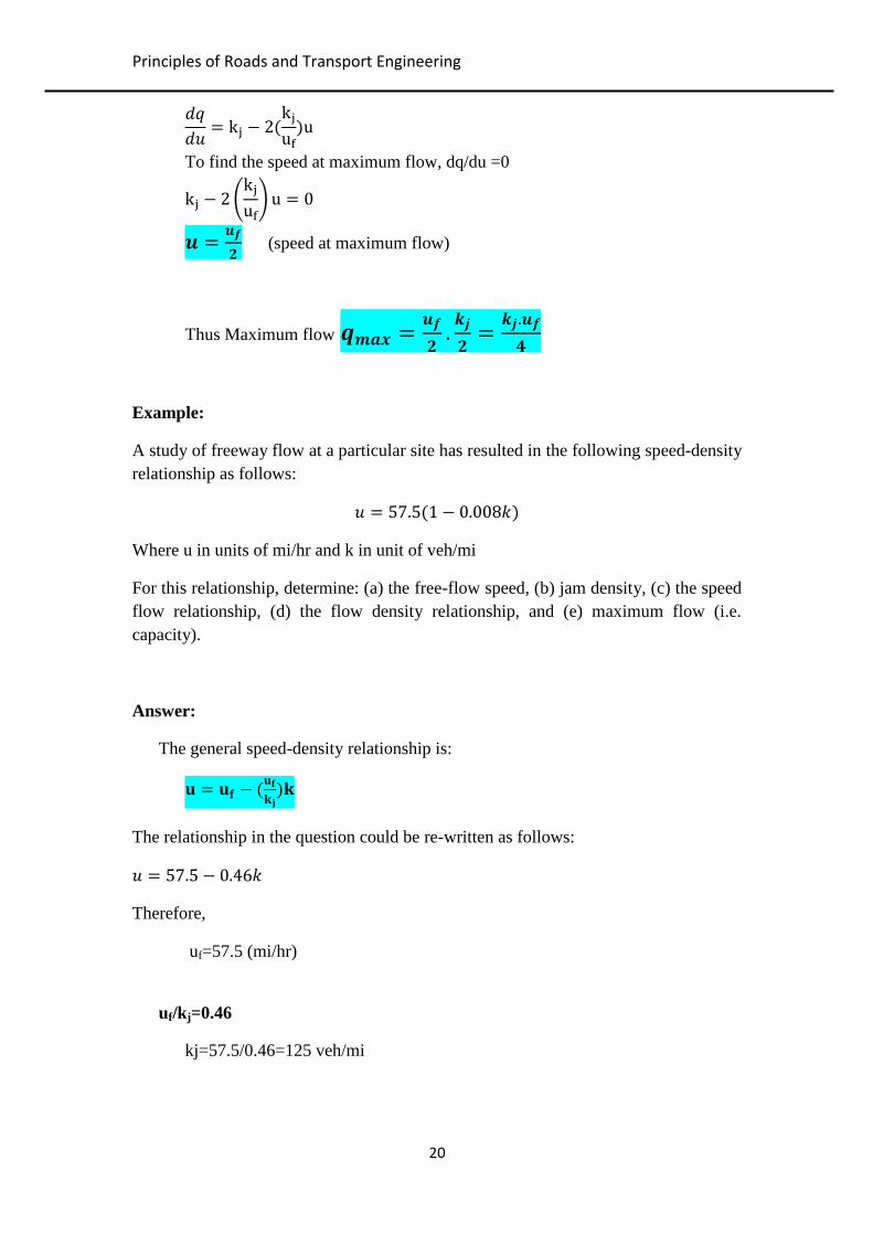
To find the speed at maximum flow, dq/du =0

(speed at maximum flow)

Thus Maximum flow

Example:

A study of freeway flow at a particular site has resulted in the following speed-density

relationship as follows:

Where u in units of mi/hr and k in unit of veh/mi

For this relationship, determine: (a) the free-flow speed, (b) jam density, (c) the speed

flow relationship, (d) the flow density relationship, and (e) maximum flow (i.e.

capacity).

Answer:

The general speed-density relationship is:

The relationship in the question could be re-written as follows:

Therefore,

uf=57.5 (mi/hr)

uf/kj=0.46

kj=57.5/0.46=125 veh/mi


21

Speed-Flow relationship

The general equation is:

By substituting kj=125 and uf=57.5 produce:

or:

, then by substituting k=q/u produces:

Flow-Density relationship

The general equation is:

By substituting kj=125 and uf=57.5 produce:

or:

then by multiplying by k produces:

Maximum flow (capacity)


22

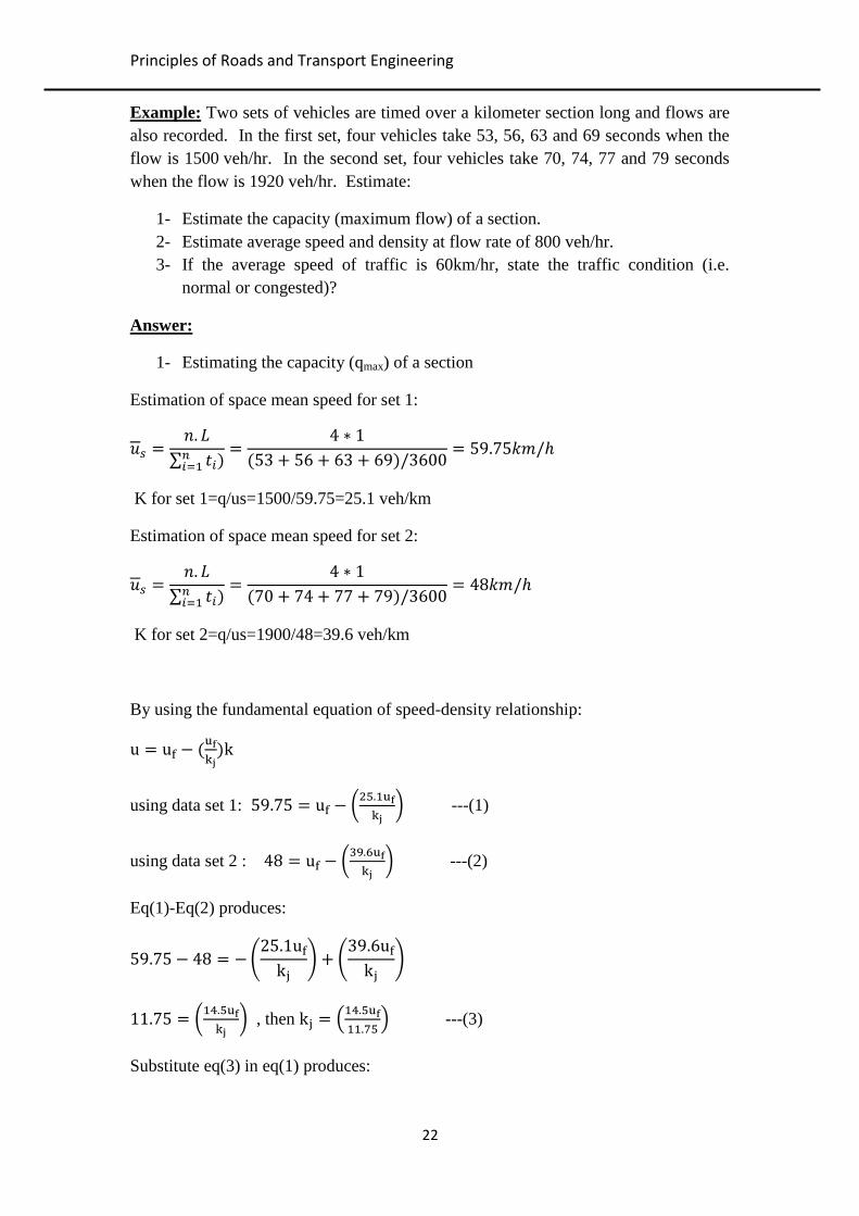
Example: Two sets of vehicles are timed over a kilometer section long and flows are

also recorded. In the first set, four vehicles take 53, 56, 63 and 69 seconds when the

flow is 1500 veh/hr. In the second set, four vehicles take 70, 74, 77 and 79 seconds

when the flow is 1920 veh/hr. Estimate:

1- Estimate the capacity (maximum flow) of a section.

2- Estimate average speed and density at flow rate of 800 veh/hr.

3- If the average speed of traffic is 60km/hr, state the traffic condition (i.e.

normal or congested)?

Answer:

1- Estimating the capacity (qmax) of a section

Estimation of space mean speed for set 1:

K for set 1=q/us=1500/59.75=25.1 veh/km

Estimation of space mean speed for set 2:

K for set 2=q/us=1900/48=39.6 veh/km

By using the fundamental equation of speed-density relationship:

using data set 1:

---(1)

using data set 2 :

---(2)

Eq(1)-Eq(2) produces:

, then

---(3)

Substitute eq(3) in eq(1) produces:


23

, then

and

2- Average speed and density at flow rates of 800 and 2000 veh/hr.

Speed at flow of 800 veh/hr

1.234u2 - 98.72u + 800 = 0

A=1.234, B= -98.72, C=800

u=70.85 at normal flow condition and u=9.15 at congested flow condition

Density at flow of 800 veh/hr

k=q/u=800/70.85=11.29 veh/km at normal flow condition

k=q/u=800/9.15=87.43 veh/km at congested flow condition

3- Since the speed of 60km/hr is higher than the speed at maximum flow of

1974veh/hr, speed at qmax=uf/2=40km/hr, then we expect that the traffic

condition is normal based on fundamental diagram of traffic flow (speed-flow

diagram)


24

Extra questions

1- 1- A traffic stream displays average vehicle headways of 2.2 s at 50 mi/h.

Compute the density and rate of flow for this traffic stream.

2- At a given location, the space mean speed is measured as 40 mi/h and the rate

of flow as 1600 pc/h/ln. What is the density at this location for the analysis

period?

3- The following counts were taken on an intersection approach during the

morning peak hour. Determine (a) the hourly volume, (b) the peak rate of flow

within the hour, and (c) the peak hour factor.


25

Capacity is the maximum hourly rate of vehicles or persons that can reasonably be

expected to pass a point, or traverse a uniform section of lane or roadway, during a

specified time period under prevailing conditions.

Demand is the principal measure of the amount of traffic using a given facility.

Demand relates to vehicles arriving while volume relates to vehicles discharging. If

there is no queue, demand is equivalent to the traffic volume at a given point on the

roadway.

Level of service (LOS) مستوى الخدمة

Level of service (LOS) is a qualitative measure describing operational conditions

within a traffic stream and their perception by drivers and/or passengers.

Types of LOS

A: free flow.

B: reasonably free flow. Maneuverability within the traffic stream is slightly restricted

C: stable flow, at or near free flow. Ability to maneuver through lanes is noticeably restricted

and lane changes require more driver awareness.

D: approaching unstable flow. Speeds slightly decrease as traffic volume slightly increase.

E: unstable flow, operating at capacity. Flow becomes irregular and speed varies rapidly.

F: forced or breakdown flow (Traffic jam)


26

Types of traffic volumes

Traffic volume is the total number of vehicles that pass over a given point or section

of a lane or roadway during a given time interval; volumes can be expressed in terms

of annual, daily, hourly, or sub-hourly periods. Traffic volume could be expressed as:

1- Average Annual Daily Traffic (AADT) is the average of 24-hour counts

collected every day of the year.

If the average annual daily traffic is not known, it can be estimated from average

weekday traffic (AWDT) using the following Equation:

2- Average Daily Traffic (ADT) is the average of 24-hour counts collected over

a number of days greater than one but less than a year.

3- Peak Hour Volume (PHV) is the maximum number of vehicles that pass a

point on a highway during a period of 60 consecutive minutes.

4- Vehicle Miles of Travel (VMT) is a measure of travel along a section of road.

It is the product of the traffic volume (that is, average weekday volume or

ADT) and the length of roadway in miles to which the volume is applicable.

VMTs are used mainly as a base for allocating resources for maintenance and

improvement of highways.


27

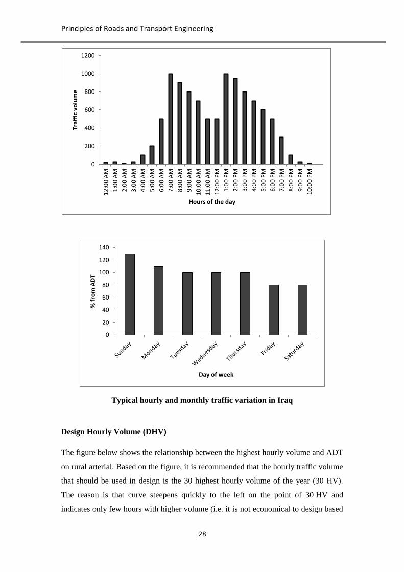
Traffic volume fluctuation

Traffic volume is changing throughout the day, the weak and the year (see following

figures for traffic volume fluctuation in Iraq and the USA).

Typical traffic variation in USA


28

Typical hourly and monthly traffic variation in Iraq

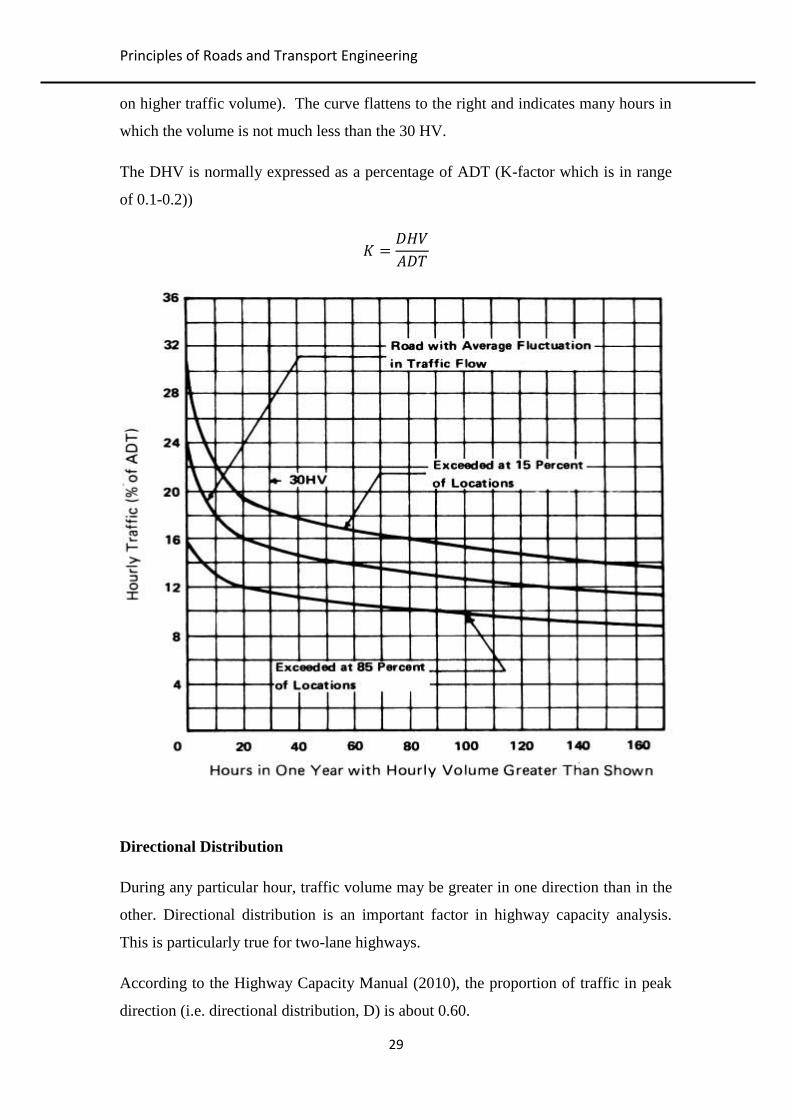
Design Hourly Volume (DHV)

The figure below shows the relationship between the highest hourly volume and ADT

on rural arterial. Based on the figure, it is recommended that the hourly traffic volume

that should be used in design is the 30 highest hourly volume of the year (30 HV).

The reason is that curve steepens quickly to the left on the point of 30 HV and

indicates only few hours with higher volume (i.e. it is not economical to design based

0

200

400

600

800

1000

1200

12

:00

AM

1:0

0 A

M

2:0

0 A

M

3:0

0 A

M

4:0

0 A

M

5:0

0 A

M

6:0

0 A

M

7:0

0 A

M

8:0

0 A

M

9:0

0 A

M

10

:00

AM

11

:00

AM

12

:00

PM

1:0

0 P

M

2:0

0 P

M

3:0

0 P

M

4:0

0 P

M

5:0

0 P

M

6:0

0 P

M

7:0

0 P

M

8:0

0 P

M

9:0

0 P

M

10

:00

PM

Traf

fic

volu

me

Hours of the day

0

20

40

60

80

100

120

140

% f

rom

AD

T

Day of week


29

on higher traffic volume). The curve flattens to the right and indicates many hours in

which the volume is not much less than the 30 HV.

The DHV is normally expressed as a percentage of ADT (K-factor which is in range

of 0.1-0.2))

Directional Distribution

During any particular hour, traffic volume may be greater in one direction than in the

other. Directional distribution is an important factor in highway capacity analysis.

This is particularly true for two-lane highways.

According to the Highway Capacity Manual (2010), the proportion of traffic in peak

direction (i.e. directional distribution, D) is about 0.60.


31

Therefore, the directional design hourly volume (DDHV) is

or

Example: a level terrain two-lane highway is expected to serve ADT of 5000 veh, find

DHV and DDHV in veh and pcu if the following information is given:

K=0.1, D=0.6

Traffic composition includes 80 passenger cars and 20% trucks.

Solution:

DHV (veh)=ADT*K

= 5000* 0.1= 500 veh

DHV (pcu)= 500*0.8*1 + 500*0.2*1.5 = 550 pcu

DDHV (veh) = ADT*K*D

=5000 * 0.1 *0.6=300 veh

DDHV (pcu) =300*0.8*1 +300*0.2*1.5 = 240 +90 =330 pcu


31

Example: The daily counts of the current traffic volume for a rural highway and for

both directions, for one week of May 2000, are as follows:

Day Saturday Sunday Monday Tuesday Wednesday Thursday Friday

Daily

volume 12000 12500 10500 11500 9500 9000 8500

The traffic composition is 70% passenger cars, 20% buses and 10% trucks. The

traffic is expected to be 180% from the current traffic up to May 2020. Find the

required number of lanes for the highway if the lane capacity is 1300 pc/hr/ln.

Assume k=0.15 and D=0.6

Answer:

ADT=sum of traffic/Number of days

Current ADT= (12000+12500+10500+11500+9500+9000+8500)/7

= 10500veh/day/2directions

المرور المستقبلي اليومي باالتجاهين

Future ADT=10500*1.8=18900 veh/day/2dir.

المرور التصميمي باالتجاهين

DHV=ADT* K=18900*0.15=2835 veh/hr/2dir.

المرور التصميمي باالتجاه الواحد

DDHV=DHV*D=2835*0.6=1701 veh/hr

DDHV (pcu/hr)=1701*0.7*1 +1701*(0.3)*1.5=1956 pcu/hr

No. of lanes=

= 1956/1300 = 1.5 lanes (use 2 lanes)


32

Public Transport system

Public transport is a shared passenger transport service which is available for use by

the general public.

General Modes of public transport:

Public transport modes include buses, trolleybuses, trams and trains, rapid

transit and ferries.

- Buses

Buses are used to carrying numerous passengers on short journeys.

- Coaches

Coaches are used to carry passengers for longer distance transportation when

compared with buses. The vehicles (coaches) are normally equipped with more

comfortable seating, a separate luggage compartment, video and possibly also a toilet.

They have higher standards than city buses, but a limited stopping pattern.

http://en.wikipedia.org/wiki/Transport_mode

http://en.wikipedia.org/wiki/Public_transport_bus_service

http://en.wikipedia.org/wiki/Trolleybus

http://en.wikipedia.org/wiki/Passenger_rail_transport

http://en.wikipedia.org/wiki/Rapid_transit

http://en.wikipedia.org/wiki/Rapid_transit

http://en.wikipedia.org/wiki/Ferry


33

- Trains

Trains are wheeled vehicles specially designed to run on railways. Trains allow high

capacity on short or long distance, but require track, signalling, infrastructure

and stations to be built and maintained.

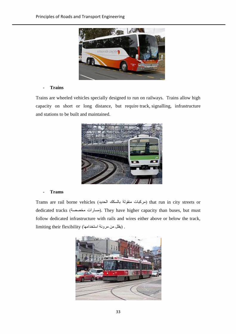
- Trams

Trams are rail borne vehicles (مركبات منقولة بالسكك الحديد) that run in city streets or

dedicated tracks ( مسارات مخصصة) . They have higher capacity than buses, but must

follow dedicated infrastructure with rails and wires either above or below the track,

limiting their flexibility ( يقلل من مرونة استخدامها) .

http://en.wikipedia.org/wiki/Track_(rail_transport)

http://en.wikipedia.org/wiki/Signalling_control

http://en.wikipedia.org/wiki/Train_station


34

- Rapid Transit

A rapid transit railway system (also called a metro or underground) operates in an

urban area with high capacity and frequency, and grade separation from other traffic.

Rapid transit systems are able to transport large amounts of people quickly over short

distances with little land use.

- Ferry

A ferry is a boat or ship, used to carry (or ferry) passengers, and sometimes their

vehicles, across a body of water. A foot-passenger ferry with many stops is sometimes

called a water bus. Ferries form a part of the public transport systems of many

waterside cities and islands, allowing direct transit between points at a capital cost

much lower than bridges or tunnels, though at a lower speed.

http://en.wikipedia.org/wiki/Grade_separation

http://en.wiktionary.org/wiki/foot-passenger

http://en.wikipedia.org/wiki/Water_bus


35

- Motorcycle

Motorcycles are used in some countries as public transportation. The motorcycles

can be used singly or with a sidecar attached, the latter often referred to as

"tricycles". They can either be hired for personal trips, like a taxi, or used for

shared trips, with set routes, like a bus.

http://en.wikipedia.org/wiki/Motorcycle

http://en.wikipedia.org/wiki/Sidecar

http://en.wikipedia.org/wiki/Tricycle_(Philippines)


36

Sight Distance on highways

Types of sight distance:

Available Sight distance (S.D)

Stopping sight distance (S.S.D)

Passing sight distance (P.S.D)

Available Sight distance (S.D): Is the length of the roadway ahead that is

visible to the driver. هي المسافة المرئية للطريق من قبل السائق

The available sight distance on a roadway should be sufficiently long to enable a

vehicle traveling at or near the design speed to stop before reaching a stationary

object.

Obstruction

يجب ان تكون كافية لتمكن السائق من التوقف حال رؤيتة جسم متوقف لالمام ( المرئية)المسافة المتوفرة

Stopping sight distance

Stopping sight distance is the sum of two distances:

(1) Reaction distance (d1): the distance traversed by the vehicle from the instant

the driver sights an object causing a stop to the instant the brakes are applied;

and

(2) Braking distance (d2): the distance needed to stop the vehicle from the instant

brake application begins.

Thus:

S.S.D=d1 + d2


37

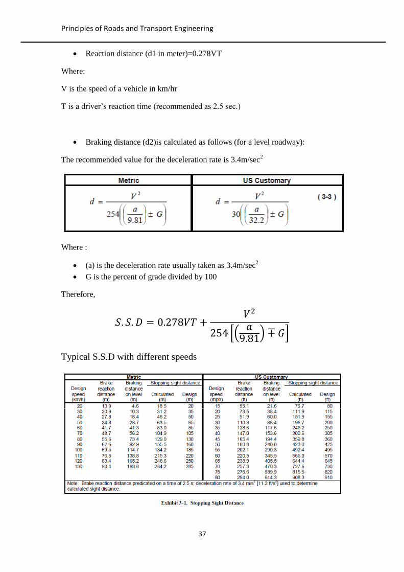
Reaction distance (d1 in meter)=0.278VT

Where:

V is the speed of a vehicle in km/hr

T is a driver’s reaction time (recommended as 2.5 sec.)

Braking distance (d2)is calculated as follows (for a level roadway):

The recommended value for the deceleration rate is 3.4m/sec2

Where :

(a) is the deceleration rate usually taken as 3.4m/sec2

G is the percent of grade divided by 100

Therefore,

Typical S.S.D with different speeds


38

Example:

The clear spacing between a vehicle and an obstruction ahead is 60m. The speed of a

vehicle is 90km/hr. Check whether this distance is satisfying the requirements of

stopping distance for the following cases:

1- level roadway

2- downgrade of -3%

3- upgrade of 3%


39

Passing sight distance on a two-lane highway

Passing sight distance is a distance required to enable drivers from passing slow

vehicles in a safe way.

The minimum passing sight distance for two-lane highways is determined as the sum of

the following four distances:

d1—Distance traversed during perception and reaction time and during the

initial acceleration to the point of encroachment on the left lane.

d2—Distance traveled while the passing vehicle occupies the left lane.

d3—Distance between the passing vehicle at the end of its maneuver and the

opposing vehicle.

d4—Distance traversed by an opposing vehicle for two-thirds of the time the

passing vehicle occupies the left lane, or 2/3 of d2 above.

1-Initial maneuver distance (d1): the distance d1 traveled during the initial

maneuver period is computed with the following equation:

Note: m is usually taken as 15km/hr.


41

2-Distance while passing vehicle occupies left lane (d2): Passing vehicles were

found to occupy the left lane from 9.3 to 10.4 sec. The distance d2 traveled in the

left lane by the passing vehicle is computed with the following equation:

3-Clearance length (d3). The clearance length between the opposing and

passing vehicles at the end of the passing maneuvers was found to vary from 30

to 75 m

Clearance distance (d3) based on speed of a passing vehicle

Speed (km/hr) 50-65 66-80 81-95 96-110

D3 (m) 30 55 75 90

4-Distance traversed by an opposing vehicle (d4): This is usually taken as

2/3d2.

Thus

Passing sight distance (P.S.D.) = d1+d2+d3+d4

Example: A driver is traveling on a two-lane highway (with speed of 90 km/hr) is

trying to overtake a vehicle ahead (with speed of 65 km/hr). The acceleration rate of

the passing vehicle is 3.1 km/hr/sec, and the vehicle spent 2.3 sec for the initial

maneuvering to the opposing lane and 8.1 sec traveling on it. If you know that the

distance between the overtaking and the opposing vehicles before the beginning of

the overtaking process is 450 meters. Is this distance adequate to complete the

overtaking process? Assume that the required clearance length between the

opposing and passing vehicle is 75m.

Solution:

P.S.D.= d1 +d2 +d3 +d4


41

d1=0.278*2.3(90-(90-65)+3.1*2.3/2)= 43.84m

d2=0.278*90*8.1=202.66m

d3=75m

d4=(2/3)*d2=(2/3)*202.66=135.1m

P.S.D. = 43.84+202.66+75+135.1=456.6m <450 this means that it is not safe to pass

the vehicle ahead.

Example: A driver is traveling on a two-lane highway (with speed of 90 km/hr) is

trying to overtake a vehicle ahead (with speed of 75 km/hr). The acceleration rate of

the passing vehicle is 3.1 km/hr/sec, and the vehicle spent 2.5 sec for the initial

maneuvering to the opposing lane and 8.0 sec traveling on it. Find the required

passing sight distance.


42

Intersections

Definition:

An intersection is defined as the general area where two or more highways join or

cross, including the roadway and roadside facilities for traffic movements within the

area.

General types of intersections;

1- At grade intersections التقاطعات السطحية

2- Interchanges- Grade separated المجسرة)التقاطعات المعزولة


43

Basic Principles of intersections design

Reduce the number of conflict points

Minimize severity of potential conflicts

Provide for smooth flow of traffic

Consider both vehicles and pedestrians

Avoid multiple and compound merging and diverging

Types and Examples of at grade intersections:

1- Three-leg/T intersections


44

2- Four-leg Intersections

3-Multi-leg Intersections


45

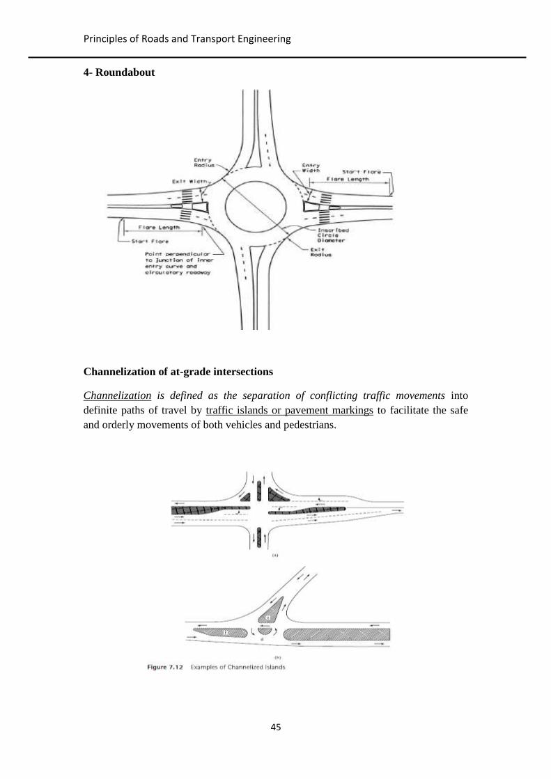
4- Roundabout

Channelization of at-grade intersections

Channelization is defined as the separation of conflicting traffic movements into

definite paths of travel by traffic islands or pavement markings to facilitate the safe

and orderly movements of both vehicles and pedestrians.


46

Importance of channelization

Channelized T intersection


47

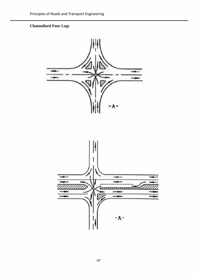
Channelized Four Legs


48

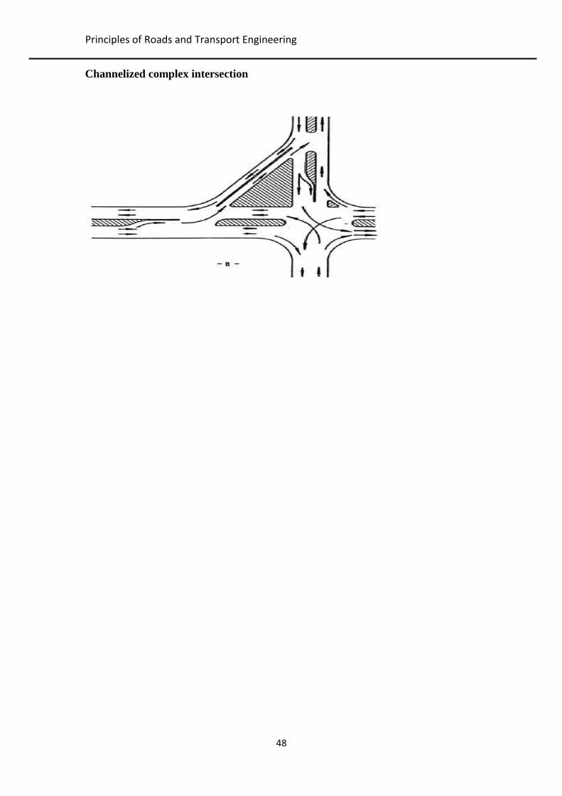
Channelized complex intersection


49

Pavement types

Main Types of Pavements are:

1- Flexible pavement

The wearing layer (top layer) in flexible pavement consists of bituminous materials.

Typical layers of flexible pavement

2- Rigid pavement

The wearing layer (top layer) in rigid pavement usually is constructed of Portland cement

concrete

Typical layers of rigid pavement

3- Block pavement

The wearing layer (top layer) in block pavement is constructed using interlocked block

pavement.


51

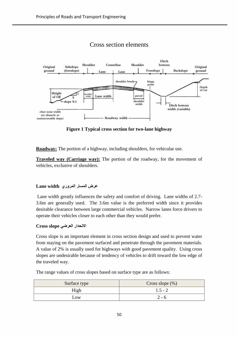
Cross section elements

Figure 1 Typical cross section for two-lane highway

Roadway: The portion of a highway, including shoulders, for vehicular use.

Traveled way (Carriage way): The portion of the roadway, for the movement of

vehicles, exclusive of shoulders.

Lane width عرض المسار المروري

Lane width greatly influences the safety and comfort of driving. Lane widths of 2.7-

3.6m are generally used. The 3.6m value is the preferred width since it provides

desirable clearance between large commercial vehicles. Narrow lanes force drivers to

operate their vehicles closer to each other than they would prefer.

Cross slope االنحدار العرضي

Cross slope is an important element in cross section design and used to prevent water

from staying on the pavement surfaced and penetrate through the pavement materials.

A value of 2% is usually used for highways with good pavement quality. Using cross

slopes are undesirable because of tendency of vehicles to drift toward the low edge of

the traveled way.

The range values of cross slopes based on surface type are as follows:

Surface type Cross slope (%)

High 1.5 - 2

Low 2 - 6


51

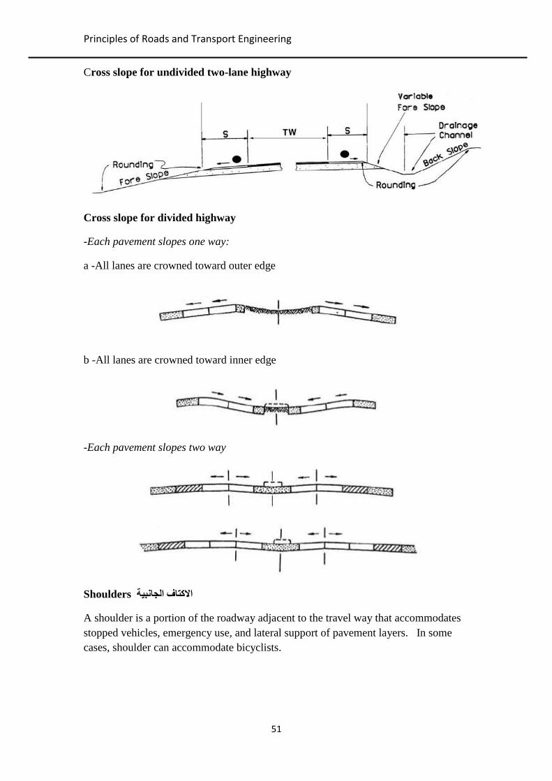
Cross slope for undivided two-lane highway

Cross slope for divided highway

-Each pavement slopes one way:

a -All lanes are crowned toward outer edge

b -All lanes are crowned toward inner edge

-Each pavement slopes two way

Shoulders االكتاف الجانبية

A shoulder is a portion of the roadway adjacent to the travel way that accommodates

stopped vehicles, emergency use, and lateral support of pavement layers. In some

cases, shoulder can accommodate bicyclists.


52

Main advantages for the use of a shoulder

Provide a space for vehicles to make emergency stop

Provide a space to avoid potential crashes or reduce their severity

The sense of openness created by shoulders of adequate width contributes to

driving ease and reduce stress

Sight distance is increased and therefore improve safety

Lateral clearance is provided for traffic sign

Storm water can be discharged farther from the traveled way, and seepage

adjacent to the traveled way can be minimized

Structural support for pavement structure

Space is provided for pedestrian and bicycle use.

Shoulder width

Shoulder width varies from 0.6m to 3.6m.

A vehicle stopped on the shoulder should clear the edge of travel way by at

least 0.3m and preferably by 0.6m. Therefore, the normal shoulder width of

3.0m is recommended.

For low-volume highways, the minimum shoulder width is 0.6m and a 1.8 to

2.4m shoulder width is preferred.

For high-volume highways carrying large numbers of trucks, the minimum

shoulder width is 3m and a 3.6m shoulder width is preferred.

Shoulders wider than 3m may encourage unauthorized use of the shoulder as a

travel lane.

Shoulder slope

Concrete and bituminous shoulders should be sloped from 2 to 6%

Crushed rock shoulders should be sloped from 4 to 6%

Median الجزره الوسطية

A median is the section of a divided highway that separates the lanes in opposing

directions. The width of a median is the distance between the edges of the inside

lanes, including the median shoulders. The functions of a median include:

Providing a recovery area for out-of-control vehicles

Separating opposing traffic

Providing stopping areas during emergencies

Providing storage areas for left-turning and U-turning vehicles

Providing refuge for pedestrians

Reducing the effect of headlight glare

Providing temporary lanes and cross-overs during maintenance operations


53

Roadside and Median Barriers

A median barrier is defined as a longitudinal system used to prevent vehicles from

crossing the portion of a divided highway separating the traveled ways for traffic in

opposite directions. Roadside barriers, on the other hand, protect vehicles from

obstacles or slopes on the roadside. They also may be used to shield pedestrians and

property from the traffic stream.

Curbs and Gutters

Curbs are raised structures made of either Portland cement concrete or bituminous

concrete (rolled asphalt curbs) that are used mainly on urban highways to delineate

pavement edges and pedestrian walkways.

Gutters or drainage ditches are usually located on the pavement side to provide the

principal drainage facility for the highway.

Right of Way

The right of way is the total land area acquired for the construction of a highway. The

width should be sufficient to accommodate all the elements of the highway cross

section, any planned widening of the highway, and public-utility facilities that will be

installed along the highway.


54

Airways Engineering:

Airways engineering is a branch of engineering science which deals with air

transportation.

Elements of Air Transportation

1) Airport is a facility where passengers connect from ground transportation to air

transportation.

2) Aircraft

3) Passengers

4) Air traffic services help in navigating aircraft while landing, taking off, flying in

the air, over-flying any country, taxing on the ground and parking.

5) Airlines: An organization that provides scheduled flights for passengers or cargo.

6) Regulations and policies: “to ensure safe and reliable trips” example: The

International Civil Aviation Organization (ICAO).

Types of Airports:

A- International:

• Has direct service to many other airports.

• Handle scheduled commercial airlines both for passengers and cargo.

• Many international airports also serve as "HUBS", or places where non-direct

flights may land and passengers switch planes.

• Typically equipped with customs and immigration facilities to handle

international flights to and from other countries.

• Such airports are usually larger, and often feature longer runways and facilities

to accommodate the large aircraft.

B-Domestic:

• A domestic airport is an airport which handles only domestic flights or flights

within the same country.

• Domestic airports don't have customs and immigration facilities and are

therefore incapable of handling flights to or from a foreign airport.

• These airports normally have short runways which are sufficient to handle

short/medium haul aircraft.


55

Main elements of a typical airport

Airports are divided into landside and airside areas. Landside areas include parking

lots, public transport railway stations and access roads. Airside areas include all areas

accessible to aircraft, including runways, taxiways and ramps. Access from landside

areas to airside areas is tightly controlled at most airports. Passengers on commercial

flights access airside areas through terminals, where they can purchase tickets,

clear security check, or claim luggage and board aircraft through gates.

Runway: A runway is a rectangular area on the airport surface prepared for the

takeoff and landing of aircraft. An airport may have one runway or several runways

which are sited, oriented, and configured in a manner to provide for the safe and

efficient use of the airport under a variety of conditions.

Taxiway: A taxiway is a path for aircraft at an airport connecting runways with

ramps, hangars, terminals and other facilities. They mostly have a hard surface such

as asphalt or concrete.

Apron: The airport apron is the area of an airport where aircraft are parked, unloaded

or loaded, refueled, or boarded. Apron is typically more accessible to users than

the runway or taxiway. However, the apron is not usually open to the general public

and a license may be required to gain access.

Terminals and gates: Terminals are used by passenger to claim boarding tickets,

clear the security check and claim their luggage. Every terminal has one or more

gates where passengers can go to the aircrafts.

Ramp: The area where aircraft parks next to a terminal to load passengers and

baggage

Hangers: Hangers is the area used for maintenance of aircrafts.

http://en.wikipedia.org/wiki/Parking_lot

http://en.wikipedia.org/wiki/Parking_lot

http://en.wikipedia.org/wiki/Public_transport

http://en.wikipedia.org/wiki/Railway_station

http://en.wikipedia.org/wiki/Road

http://en.wikipedia.org/wiki/Taxiway

http://en.wikipedia.org/wiki/Airport_ramp

http://en.wikipedia.org/wiki/Airport_terminal

http://en.wikipedia.org/wiki/Airport_security

http://en.wikipedia.org/wiki/Baggage_claim

http://en.wikipedia.org/wiki/Gate_(airport)

http://en.wikipedia.org/wiki/Aircraft

http://en.wikipedia.org/wiki/Airport

http://en.wikipedia.org/wiki/Runway

http://en.wikipedia.org/wiki/Airport_ramp

http://en.wikipedia.org/wiki/Hangar

http://en.wikipedia.org/wiki/Airport_terminal

http://en.wikipedia.org/wiki/Asphalt

http://en.wikipedia.org/wiki/Concrete

http://en.wikipedia.org/wiki/Airport

http://en.wikipedia.org/wiki/Aircraft

http://en.wikipedia.org/wiki/Runway

http://en.wikipedia.org/wiki/Taxiway


56

Typical Airport layout


57

Aircraft characteristics affecting airports design:

A) Aircraft dimensions

B) Aircraft Weight

C) Engine types

principles of roads and transport engineeringqu.edu.iq/eng/wp-content/uploads/2015/10/... ·...

Documents