principles of single-molecule … manipulation in biological physics cytoplasm cytoskeleon filament...

April 30, 2012 11:8 WSPC/Guidelines-IJMPB S021797921230006X

International Journal of Modern Physics BVol. 26, No. 13 (2012) 1230006 (21 pages)c© World Scientific Publishing Company

DOI: 10.1142/S021797921230006X

PRINCIPLES OF SINGLE-MOLECULE MANIPULATION

AND ITS APPLICATION IN BIOLOGICAL PHYSICS

WEI-HUNG CHEN∗,†, JONATHAN D. WILSON∗, SITHARA S. WIJERATNE∗,

SARAH A. SOUTHMAYD∗, KUAN-JIUH LIN† and CHING-HWA KIANG∗,‡

∗Department of Physics and Astronomy, Rice University, Houston, Texas 77005, USA†Department of Chemistry, National Chung Hsing University, Taichung, Taiwan

‡[email protected]

Received 8 March 2012Published 30 April 2012

Recent advances in nanoscale manipulation and piconewton force detection provide aunique tool for studying the mechanical and thermodynamic properties of biologicalmolecules and complexes at the single-molecule level. Detailed equilibrium and dynamicsinformation on proteins and DNA have been revealed by single-molecule manipulationand force detection techniques. The atomic force microscope (AFM) and optical tweezershave been widely used to quantify the intra- and inter-molecular interactions of manycomplex biomolecular systems. In this article, we describe the background, analysis, andapplications of these novel techniques. Experimental procedures that can serve as a guidefor setting up a single-molecule manipulation system using the AFM are also presented.

Keywords: Single-molecule; AFM; biomolecule.

1. Introduction

Over the last few years, studying the role of mechanics in biomolecules has

helped us gain insight into the mechanochemical transduction inside and outside

cells.1,2 The mechanical properties of biomolecules may also play an essential role

in understanding the interplay between mechanics and biochemistry. Since Isaac

Newton wrote his three laws of motion more than three centuries ago, great progress

has been made in mechanics. There is now increasing evidence that mechanics plays

an important role in advancing life science and medicine.3 The connection between

mechanics and biological functions has become a subject of broad interest.

Like an error-free factory at the nanoscale, molecular machines in biological

systems perform specific functions induced by tiny forces. When forces are applied

to these biomolecules, their conformations change in response to the load. It is

well-established that the three-dimensional structure of the biomolecule defines

‡Corresponding author.

1230006-1

http://dx.doi.org/10.1142/S021797921230006X

mailto:[email protected]


W.-H. Chen et al

its function. However, the conformations of biomolecules change constantly within

their biological systems, thus studying biomolecular properties via mechanics will

illuminate their dynamics and functions. Information about the kinetics of the

conformational changes will allow us to understand how their structural changes

trigger biological reactions. Recently, due to advances in nanotechnology, methods

such as AFM and optical tweezers for measuring the forces in individual molecules

have been developed to investigate the kinetics of these conformational changes,

thereby linking their mechanical response with biochemical function.

1.1. Mechanics of biological systems

1.1.1. Cell mechanotransduction

Cells, the basic units of life, are complex biological systems. Recently, studies have

shown that the mechanical environment may play a regulatory role in cellular

functions.4–7 Therefore, studying the mechanical properties of cells may shed light

on their biological functions. One example is bone tissue, which is continuously

constructed and destroyed by two bone cells, osteoblast and osteoclast.8,9 The

dynamic equilibrium of this bone remodeling cycle controls bone gain and loss,

and dysregulation of this equilibrium is linked to osteoporosis.9 Recent studies on

astronauts have suggested that mechanical force plays an important role in the

regulation of bone metabolism.10 These studies reveal that working in weightless

environments can cause a loss of bone density at up to 1–2% each month,6 ten

times faster than that of osteoporosis patients on Earth. Weight-bearing exercises

effectively slow this decay rate, implying that force (gravity) is a key regulator of

bone metabolism.11

Another well-known example of mechanical regulation is the endothelial cell,

which forms the interior surface of blood vessels and responds rapidly to mechanical

forces. Studies have shown that vascular morphology and physiology are largely

determined by blood flow,5,12 and that endothelial cells are the components that

mediate this effect. In a healthy blood vessel, laminar shear forces from blood

flow make endothelial cells align along the walls of the vessel. In contrast, slow or

turbulent blood flow activates endothelial cells and increases their turnover rate,

resulting in substantial disordered cells, cell retraction, or cell loss and hence the

early development of vascular diseases, such as atherosclerosis.

1.1.2. Elasticity of biomolecules

To determine how cells convert mechanical forces into biochemical signals, an

investigation of the biomolecules inside the cells is necessary. A cell is wrapped with

the plasma membrane and braced by the cytoskeleton, which consists of filament

proteins that serve as intracellular scaffolds to support the cell’s shape4 (see Fig. 1).

The conformational changes of the cytoskeleton alter the tension and the structure

of the cell. In a physiological environment, cells are attached to the extracellular

1230006-2


Single-Molecule Manipulation in Biological Physics

cytoplasmcytoskeleon filament

plasma membrane

Fig. 1. A cell attaches to the ECM through the binding between ECM proteins, such asfibronectin and integrin and the intracellular domain, which couples to the cytoskeleton.4 Adaptedfrom Ref. 4.

matrix (ECM) through the binding between the ECM proteins and the receptor

proteins on the cell surface.13

Integrin, a transmembrane protein attached to the cell cytoskeleton, is crucial

to the adhesive stability between the cell and the ECM or other cells. Since

integrins provide the mechanical linkage between the cell cytoskeleton and

ECM, cytoskeleton systems can sense mechanical forces through integrin-mediated

cell-ECM interactions and change their structure to generate intracellular force

to resist the load.14 How the mechanical properties of cytoskeleton proteins affect

the biochemical reactions inside the cell remains unknown. However, it has been

suggested that the deformation of the cytoskeleton might modify its affinity with the

proteins attached to it.15 This affinity modification could then induce the alteration

of structures and functions of the attached proteins, thus changing the downstream

biochemical processes throughout the cytoplasm and nucleus.16

The cytoskeleton is not the only example which shows the coupling of mechanics

and biochemistry. Other examples include the folding of two or more globular

clusters (domains) and the deformation or unfolding of the globular domains in

the ECM protein fibronectin under stretching forces. When cells apply tensile

or contractile forces to the ECM, fibronectins unfold and refold, respectively.17

It has been proposed that the folding and unfolding states of fibronectins may

have significant implications to cell signaling, since different fibronectin structures

regulate the fibronectin–integrin binding or establish a mechanosensitive ligand

recognition system.18

The elastic properties of DNA have also attracted attention due to DNA’s

importance in storing genetic information. The arrangement of the four DNA

bases, i.e., adenosine, cytidine, guanosine and thymidine, provides the code to

produce proteins. However, not all sequences encode genetic information. Some

DNA sequences serve as recognition sites for DNA-binding proteins, like the TATA

box,19 which labels the starting position of transcription.20 To understand why

base sequences have specific affinities for certain proteins, the rigidity of DNA has

1230006-3


W.-H. Chen et al

Rupture of

covalent bonds

B ond angle deformation

Supramolecular reorganization

kB T = 4.1 pN nm

Entropic elasticity

Force (pN)

Le

ng

th (

nm

)

>10

1

0.1

50 0505

Fig. 2. Accessible force window of single-molecule manipulation.34 The white area shows theexperimental accessibility of mechanical information. From Ref. 34.

been studied extensively,21–23 including the sequence dependence of the stiffness of

DNA.24–26

1.2. Single-molecule manipulation

Since Feynman proposed the idea of the molecular machine in his famous speech

“There’s Plenty of Room at the Bottom” in 1959,27 nanoscience and nanotechnology

have advanced into technology-based research, opening the door for the precise

manipulation of objects on the atomic scale. Recent developments in single-molecule

manipulation have created new research in many fields such as physics, chemistry,

materials science, biology, medicine and engineering. A number of techniques that

can be applied to measure tiny forces are available: The most prominent of which

are the AFM,28,29 optical tweezers,30 magnetic tweezers,31 glass microneedles,32

and the biomembrane force probe.33 Within the accessible force window,34 the

range from measuring the entropic elastic force (several femtonewtons) to breaking

covalent bonds (a few nanonewtons) can now be studied (Fig. 2).

1.2.1. Atomic Force Microscopy (AFM)

To improve the microscope resolution beyond the Abbe barrier of 200 nm using

visible light, Binnig et al., of IBM Zurich research laboratory, proposed a new

scanning probe microscope in 1986, i.e. the AFM.35 An AFM probe attached to an

ultra-soft cantilever senses the force between atoms of the probe and the surface.

1230006-4



Fig. 3. Experimental set-up of the first generation AFM. From Ref. 35.

In the prototype AFM (Fig. 3), a scanning tunneling microscope (STM) probe

monitored the bending of the cantilever, with a feedback control system which

controlled the vertical movement of the scanner to keep the force on the AFM

probe constant while it raster scanned over sample surfaces. The surface topography

was then reconstructed from the vertical movement of the scanner. In 1987, a new

method to measure the bending of the AFM cantilever based on the optical lever

mechanism was proposed.36 This optical system has now replaced STM probes as

the most popular AFM probe displacement sensor.

When the operating force during AFM scanning is high, the interaction between

the tip and the surface produces a deformation on soft film,37 which inspired

researchers to use AFM tips to manipulate microscopic objects. AFM tips were used

to modify the surface38,39 or to move nanomaterials to construct arbitrary nanoscale

patterns.40 This technique opened up new possibilities in manipulating materials

for nanoscience and nanotechnology. Thus, the AFM is not only a detector, but

also a nanostructure constructor and manipulator.

Taking advantage of the capability of AFM to measure the force applied onto the

tip while manipulating the object, the first biological force measurement using AFM

was demonstrated in 1994.28 AFM tips were functionalized with avidin to measure

the adhesive force of agarose beads modified with biotin to extract the avidin–biotin

specific binding force. AFM was later used to investigate the mechanical and

thermodynamic properties of biomolecules. For example, a giant sarcomere muscle

protein was picked up by an AFM probe and stretched (Fig. 4). The force exerted

on the molecule as a function of extension was recorded and the resulting sawtooth

patterns were attributed to the unfolding of individual domains.28

Unlike optical tweezers, where the biomolecule was held between two beads

via molecular handles, the AFM tip attaches to the biomolecule via nonspecific

binding. This allows AFM to apply higher forces to the biomolecule than with

optical tweezers. In addition, the force curve obtained using AFM does not include

1230006-5


W.-H. Chen et al

Laser

Position-sensitive

photosensor

AFM cantilever

(a) (b)

Fig. 4. Detection principles of AFM. (a) The bending of the AFM cantilever induced by theforce applied to the tip is magnified and determined from the laser beam deflection on theposition-sensitive photosensor. (b) The AFM cantilever is assumed to act as a harmonic potentialthat applies force onto a molecule. From measuring the vertical displacement of the cantilever andthe spring constant, the force exerted on the molecule is calculated.

the contribution from the DNA handles, whereas in optical tweezers, the elastic

properties of handle molecules must be decoupled from the force curves.

1.2.2. Optical tweezers

In 1987, Ashkin et al. first used optical tweezers to move cells under a damage-free

condition.41 Optical tweezers use the force generated by the radiation pressure of a

focused laser light beam, with the gradient force keeping the micrometer size beads

in the high intensity region of the light beam42,43 (Fig. 5). This gradient force

is effective in manipulating particles from the micrometer-scale particles down to

individual atoms.44,45 The first generation of the experimental set-up consisted of

a 1.06 µm wavelength neodymium-doped yttrium aluminium garnet laser focused

onto a viewing plane with a water-immersion objective lens to form a single-beam

optical trap. After being trapped in the focal spot, the position of the biological

cell can be controlled by moving the X,Y,Z microscope sample stage. Ashkin et

al. also separated individual bacteria from one sample and introduced them into

another, demonstrating the potential of performing cell surgery using this optical

technique.41

Optical tweezers were used to measure the force-extension curves of individual

double-stranded DNA (dsDNA) molecules in 1996.30 Each end of the dsDNA

molecule was coupled with a micrometer size latex bead, with one bead held by

a glass micropipette and the other bead held in the optical trap. The dsDNA

molecule was extended by moving the pipette away from the laser trap. The change

in dsDNA length was monitored by recording the distance between two beads with a

video camera. They adopted a new optical tweezer design where the force acting on

1230006-6



1 2

F2

F1

Fnet

Pout

Pin

Pchange

Pparticle

(a) (b)

Fig. 5. The operating principles of optical tweezers.41 (a) The change in scattering photonmomentum (Pchange = Pout − Pin) produces an opposite momentum change on the particle(Pparticle) according to Newton’s third law. (b) Different shades of red represent differentintensities light. When the particle is displaced from the beam center, the net force of the radiationpressure exerted on the particle points toward the beam waist.

the dsDNA molecule corresponding to each extension could be directly determined

from the angular intensity distribution of the laser beams on position-sensitive

photodetectors.46 Removing the need for complicated calibration,47 this direct

method to measure the force exerted by optical tweezers remains popular.

Recent developments have improved the stability and reduced the noise

in optical tweezers.48 Many hybrid systems have been proposed, significantly

expanding the capabilities of traditional optical tweezers. These include multiple

optical traps,49 optical tweezers coupling with rotational control,50 and fluorescence

optical tweezers,32 enabling the manipulation of more complex biological systems.

2. Methods

2.1. AFM experiments

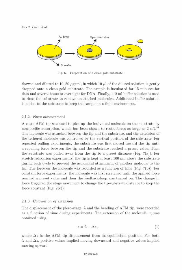
2.1.1. Sample preparation

One way to obtain a clean gold substrate for an AFM substrate is to have an AFM

specimen disc adhered to a commercial silicon wafer coated with a gold layer by

epoxy glue, which is left to dry for one day (Fig. 6). The AFM specimen disc is

then carefully peeled away from the silicon wafer prior to sample attachment.

To prepare the sample solution, the molecules are diluted with a buffer solution

at 100 µg/ml concentration with 150 mM NaCl, similar to physiological conditions.

For titin, the buffer is phosphate buffer saline (PBS) solution. For DNA, the buffer

is tris-HCl buffer solution containing 1 mM EDTA. This concentrated sample is

stored at −20◦C. To use the sample for experiments, the frozen sample solution is

1230006-7


W.-H. Chen et al

Au layer

Si wafer

Specimen disk

Fig. 6. Preparation of a clean gold substrate.

thawed and diluted to 10–50 µg/ml, in which 10 µl of the diluted solution is gently

dropped onto a clean gold substrate. The sample is incubated for 15 minutes for

titin and several hours or overnight for DNA. Finally, 1–2 ml buffer solution is used

to rinse the substrate to remove unattached molecules. Additional buffer solution

is added to the substrate to keep the sample in a fluid environment.

2.1.2. Force measurement

A clean AFM tip was used to pick up the individual molecule on the substrate by

nonspecific adsorption, which has been shown to resist forces as large as 2 nN.51

The molecule was attached between the tip and the substrate, and the extension of

the tethered molecule was controlled by the vertical position of the substrate. For

repeated pulling experiments, the substrate was first moved toward the tip until

a repelling force between the tip and the substrate reached a preset value. Then

the substrate was pulled away from the tip to a preset distance (Fig. 7(a)). For

stretch-relaxation experiments, the tip is kept at least 100 nm above the substrate

during each cycle to prevent the accidental attachment of another molecule to the

tip. The force on the molecule was recorded as a function of time (Fig. 7(b)). For

constant force experiments, the molecule was first stretched until the applied force

reached a preset value and then the feedback-loop was turned on. The change in

force triggered the stage movement to change the tip-substrate distance to keep the

force constant (Fig. 7(c)).

2.1.3. Calculation of extension

The displacement of the piezo-stage, λ and the bending of AFM tip, were recorded

as a function of time during experiments. The extension of the molecule, z, was

obtained using,

z = λ−∆z , (1)

where ∆z is the AFM tip displacement from its equilibrium position. For both

λ and ∆z, positive values implied moving downward and negative values implied

moving upward.

1230006-8



(a)

(b)

(c)

Repeat until detachment

Constant force

Constant force

Constant force

Fig. 7. (a) Typical pulling experiments where the movement of the substrate is controlled by thepiezo-electric stage. (b) Stretch-relaxation experiments. After a molecule is picked up by the AFMtip, it is stretched and relaxed repeatedly. (c) Constant force experiments. A molecule is pickedup and it is stretched until the force reaches a preset value and then the force is kept constant.

2.2. Equilibrium free energy curve reconstruction

2.2.1. Jarzynski’s equality

Since stretching a molecule is not an equilibrium process, the free energy changes

cannot be directly obtained by calculating the work applied to the molecule.

However, in 1997, Jarzynski derived an equation which relates the work, W , to

the free energy change, ∆G,52

〈exp(−βW )〉n→∞ = exp(−β∆G) , (2)

where β ≡ 1/kBT , kB is the Boltzmann constant, T is the temperature and 〈. . .〉N is

the average overN realizations. The equality is exact whenN → ∞, which indicates

that the free energy change can be determined by the work done in single-molecule

manipulation experiments.

2.2.2. Velocity dependence

Jarzynski’s equality52,53 shows great potential as a method for obtaining

the free energy change from nonequilibrium single-molecule force-extension

1230006-9


W.-H. Chen et al

100 1000N

0.02

0.05

0.10

0.20

0.50

1.00

2.00

5.00

Ve

locity (

µm

/s)

1 10

Fig. 8. Free energy convergence as a function of pulling velocity.61 The number of realizations, N,required to converge to within 10% of the averaged free energy was found to depend exponentiallyon the pulling velocity. From Ref. 61.

measurements.54−59 The equality promises to recover the free energy changes

from single-molecule pulling experiments at any pulling velocity, given enough

realizations.60 However, the equality is strictly valid only in the limit of infinite

realizations. Therefore, practical use of Jarzynski’s equality requires that the

number of realizations needed for an accurate approximation is reasonable for its

practical application in experiments.

Figure 8 shows the number of realizations, N , necessary to calculate ∆G

within 10% of the converged values as a function of pulling velocity.61 N increases

exponentially with velocity, so that excessively high pulling velocities call for

impractical numbers of realizations.60 High velocity results may also be affected by

hydrodynamic drag.62 On the other hand, pulling at very slow velocities introduces

systematic error from instrument drift. Therefore, velocities between 0.2 µm/s and

1.0 µm/s appear to be optimal.60

2.2.3. Is end-to-end distance a good reaction coordinate?

While single-molecule manipulation has made much progress in recent years,63,64

the important relationship between the thermal, mechanical and chemical process

is still a subject of debate. The question is not whether the mechanical or chemical

method more faithfully resembles the process in vivo, since both methods present

results in the zero-perturbation limit, i.e. the zero force or zero chemical denaturant

condition. The external perturbation changes the free energy landscapes, similarly

for bulk chemical denaturants and single force measurements, implying that the

1230006-10



U

F T

Fig. 9. The solid and dashed lines indicate the pathways of force and chemical induced unfolding,respectively.60 Unlike chemical experiments, where the process is expressed in terms of the reactioncoordinate, the force measurement has one additional constraint, i.e. the molecular end-to-enddistance. From Ref. 60.

energy pathways of these two methods are close to each other (Fig. 9), thus

supporting the notion that the end-to-end distance is a good reaction coordinate.

3. Application to Biomolecules

3.1. Titin: Protein polymer physics and thermodynamics

Titin is a giant protein responsible for generating passive retraction forces in muscle

cells. This protein connects the M-line and Z-line of the sarcomere, stabilizing its

structure and preventing it from being overstretched during muscle expansion. Titin

consists of three spring elements: Ig (serially linked immunoglobulin-like domains),

PEVK (rich in proline, glutamate, valine and lysine) and an N2B domain (only

for cardiac muscles) (Fig. 10).65,66 Several of the Ig domains, particularly, the I27

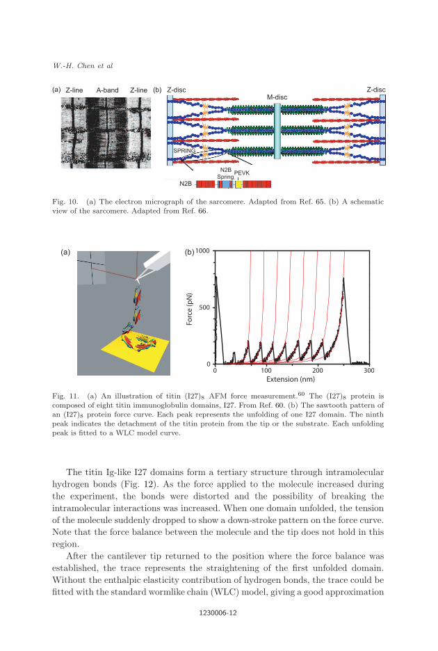
domains, have been studied extensively with the AFM [Fig. 11(a)] and optical

tweezers.67,68

Figure 11(b) displays the force-extension curve of the titin (I27)8 molecule. The

first peak in the force curve can be attributed to the nonspecific binding force

between the tip and the substrate. Upon stretching, the force increased with the

movement of the substrate because of the entropy reduction resulting from the trend

to align the molecule with the pulling direction. In the case of Fig. 11(b) where all

eight domains were in the folded state before pulling, the globular domains were

straightened without having initially unfolded.

1230006-11


W.-H. Chen et al

Z-line A-band Z-line(a) (b) Z-disc Z-discM-disc

N2B

N2B

SpringPEVK

SPRING

Fig. 10. (a) The electron micrograph of the sarcomere. Adapted from Ref. 65. (b) A schematicview of the sarcomere. Adapted from Ref. 66.

100 200 3000

500

1000

Fo

rce

(p

N)

Extension (nm)

(b)(a)

0

Fig. 11. (a) An illustration of titin (I27)8 AFM force measurement.60 The (I27)8 protein iscomposed of eight titin immunoglobulin domains, I27. From Ref. 60. (b) The sawtooth pattern ofan (I27)8 protein force curve. Each peak represents the unfolding of one I27 domain. The ninthpeak indicates the detachment of the titin protein from the tip or the substrate. Each unfoldingpeak is fitted to a WLC model curve.

The titin Ig-like I27 domains form a tertiary structure through intramolecular

hydrogen bonds (Fig. 12). As the force applied to the molecule increased during

the experiment, the bonds were distorted and the possibility of breaking the

intramolecular interactions was increased. When one domain unfolded, the tension

of the molecule suddenly dropped to show a down-stroke pattern on the force curve.

Note that the force balance between the molecule and the tip does not hold in this

region.

After the cantilever tip returned to the position where the force balance was

established, the trace represents the straightening of the first unfolded domain.

Without the enthalpic elasticity contribution of hydrogen bonds, the trace could be

fitted with the standard wormlike chain (WLC) model, giving a good approximation

1230006-12



Hydrogen

bonds

Fig. 12. Three-dimensional structure of the titin I27 protein.

0 2 4 6 8 10 120

100

200

300

400

Lp=0.5 nmLp=0.4 nm

Lp=0.3 nm

Lp=0.2 nm

Lp=0.1 nm

Fo

rce

(p

N)

Extension (nm)

Fig. 13. Comparison of WLC model curves with respect to persistence length. The temperatureis 300K and the contour length is 12 nm in the five WLC curves.

to describe the entropic elasticity of a polymer,69

FLp

kBT=

z

Lc

+1

4(1− zLc

)2−

1

4, (3)

where F is the force, Lc is the contour length and Lp is the persistence length, a

parameter describing the rigidity of a polymer (Fig. 13). In the case of titin, the

persistence length is the size of one amino acid, 0.4 nm, and the contour length of

each domain is 28 nm.29,70

As the molecule was extended, domains of a titin (I27)8 molecule unfolded

one by one, resulting in a sawtooth pattern. The last peak, [Fig. 11(b)], with a

much higher force peak than the unfolding peaks, represents the detachment of the

protein. Because the molecule is randomly picked up by the cantilever tip, not all

the force-extension curves show the intact force curve like Figure 11(b). Figure 14

shows variations with fewer numbers of unfolding peaks and unfolding forces within

1230006-13


W.-H. Chen et al

0 50 100 150 200

0

100

200

300

400

Fo

rce

(p

N)

Extension (nm)

0

100

200

300

Fo

rce

(p

N)

Extension (nm)

0

100

200

300

400

500F

orc

e (

pN

)

Extension (nm)

0

100

200

300

400

Fo

rce

(p

N)

Extension (nm)

(a) (b)

(c) (d)

500 100 150 2000 50 100 150 200

0 50 100 150 200

Fig. 14. Typical force-extension curves of a titin (I27)8 molecule. The red lines are WLC modelfits to the data.

the force curve. This indicates that the unfolding event is a stochastic process.70

Considering the unfolding as a zero-order reaction, the lifetime of the distorted titin

I27 domain,71 τ , is,

1

τ= ku(F ) ∼ exp

−(∆G‡u − F∆x‡)

kBT, (4)

where ku(F ) is the reaction rate constant, ∆G‡ is the free energy barrier for

unfolding and ∆x‡ is the distance between the native and transition states. The

probability of unfolding increases with increasing applied force.

The cross correlation function was used to align force-extension curves by

shifting them along the extension-axis,

r =

∑

i[(xf (i)− 〈xf 〉)× (yf (i − d)− 〈yf 〉)]√∑

i(xf (i)− 〈xf 〉)2√∑

i(yf (i − d)− 〈yf 〉)2, (5)

where xf and yf are two force curve fits to the WLC model. After the d for the

maximum r was found, the force and extension data of y were shifted by d data

points. This method has been used to align the force curve obtained from the same

kind of molecule with different contour lengths.54,57 The geometric error due to the

deviation of the pulling direction from the vertical line normal to the substrate has

proven to be less than 1%.70 Therefore, the reproducibility of the titin force curve

can be confirmed by the good overlap among the force-extension curves (Fig. 15).

Figure 16 depicts the statistics of the data. The average increase in contour

length from the first to the second peak was 28 nm, which is close to the expected

maximum length change of 29 nm from the unraveling of an I27 domain.72,73 The

analysis also shows that the domain length, defined as the peak-to-peak distance,

1230006-14



500

1000

Fo

rce

(p

N)

Extension (nm)

500

1000

500

1000

0

200

400

600

800

Fo

rce

(p

N)

Extension (nm)

(a) (b)

0 100 200 300 0 100 200 300

Fig. 15. Overlay of titin force-extension curves. The force-extension curve is shifted along theextension-axis according to cross correlation functions. The overlay shows that the second peaksof three selected force-extension curves are well overlapped.

25 300

10

20

30

Co

un

t

Change in contour length (nm)

15 20 250

10

20

30

Co

un

t

Domain length (nm)

100 200 300 4000

10

20

30

Co

un

t

Force Peak Height (pN)

Fig. 16. Histograms of the contour length difference between the first and the second peak, lengthof the second domain, and the force of the second peak height. The contour length was obtainedfrom WLC fitting curves. The pulling velocity is 1 µm/s.

20 nm, is shorter than the contour length. Thus, the unfolded chain could not

fully extend before the next domain unfolded. At a pulling speed of 1 µm/s,

the force peaks ranged from 120 to 350 pN, with an average force of 235 pN.

The unfolding force depends on the mechanical stability of the folded molecule

and pulling velocity.54 Repeated pulling experiments show a distribution in force

peaks. Stretch-relaxation of the same molecule eliminates the variety caused by

the geometric error.70 However, the molecule may fail to refold after several cycles,

thereby increasing the difficulty in collecting a complete set of data.

Reconstruction of free energy surfaces was done using the method described in

Ref. 54. In brief, the second peaks were extracted from a titin (I27)8 force curve and

aligned using cross correlation functions [see Eq. (6)]. Each of the N integration

curves was split into S segments and the free energy difference between the starting

point of the integration and the midpoint of the mth segment was calculated using,

exp[−β∆G(zm)] ≈1

NS

N∑

i=1

S∑

j=1

δǫ(zm − zi,j)× exp(−βWi,j) , (6)

where zi,j is the extension of the molecule at the jth data point for the ith trajectory

and Wi,j is the work performed up to this data point. δǫ is 1/ǫ when zi,j falls inside

1230006-15


W.-H. Chen et al

0 10 20 300

100

200

300Average Work

Free energy using Jarzynski estimator

En

erg

y (

kca

l/m

ole

)

Extension (nm)

(a) (b) (c)

Reaction coordination

Fre

e E

ne

rgy

G =7.5

kcal/mole

G =11.4

kcal/mole

Folding state

Transition state

Unfolding

state

G =3.9

kcal/mole100 200 300

0

10

20

30

Co

un

t

Work (kcal/mole)

100 200 3000

10

20

30

Co

un

tWork (kcal/mole)

Fig. 17. Free energy curve of titin I27 proteins.54 (a) The free energy curves were reconstructedusing the Jarzynski’s equality and arithmetic mean. (b) The distribution of the work done until0.6 nm before the peak (upper) and at the peak (lower). (c) The free energy diagram of the titin

unfolding/folding process. ∆G‡u was obtained from the free energy surface reconstructed using

Jarzynski’s equality, assuming the distance between the folded and the transition states is 0.6 nm.Adapted from Ref. 54.

the mth segment and 0 otherwise. Figure 17 shows the reconstructed free energy

curve along the end-to-end distance coordinate. The averaged work curve, 〈W 〉 =1NΣN

i=1Wi displayed in Fig. 17 for comparison, is about twice that of Jarzynski’s

averaged free energy curve.

Assuming the length difference between the native state and the transition state

of I27 protein is 0.6 nm,74 the energy barrier for unfolding, ∆G‡, can be obtained

from the free energy curve, 11.4 kcal/mole. In the downstoke region, the assumption

that the force on the molecule equals the restoring force of the cantilever no longer

holds. Therefore, the free energy curve is not accurate after the transition state.

However, using the unfolding free energy change, ∆Gu = 7.5 kcal/mol, determined

by other equilibrium studies,75 the energy barrier for folding, ∆G‡f , was determined

to be 3.9 kcal/mole, which is in the expected range for I27, thus further validating

this method.

3.2. DNA mechanics and melting

3.2.1. Melting of double-stranded DNA

AFM has also been used to study the mechanical melting of dsDNA, as shown

in Fig. 18. λ-DNA is a dsDNA, having normal distributions of base sequences.

Therefore, the segments randomly picked up by the AFM have no effect on the

results. The force curves show two distinct features at 65 pN and near 150 pN, which

are attributed to the B–S transition and dsDNA melting, respectively.30,76−80

The B–S transition is the transition from the B -form DNA to a metastable

S -form. B -form DNA is the double helix structure formed by Watson–

Crick base pairing. During pulling experiments, when the B -form λ-DNA is

overstretched, the dsDNA no longer adopts the B -form structure and undergoes

conformational changes including base unstacking and the unwinding of the helix

structures.30,78 The three conformations of λ-DNA during pulling, B -DNA, S -DNA

1230006-16



0

100

200

300

Fo

rce

(p

N)

Raw dataB-DNA WLCS-DNA WLCssDNA FJC

1.0 1.5 2.0

Extension (µm)

Fig. 18. Force-extension curve of dsDNA.76 The dsDNA force curve is fitted to theextensible WLC and the extensible freely-jointed chain (FJC) models to describe three differentconformations during stretching. B-DNA and S-DNA are fitted using the extensible WLC modelwith different parameters. Single-stranded DNA (ssDNA) is fitted using the extensible FJC model.From Ref. 76.

ExtensionRecA

SSB

Fig. 19. During DNA recombination, dsDNA was coated by RecA proteins and was extendedby 50% before the exchange of DNA strands and the homology search.86 This process does notrequire ATP hydrolysis. Adapted from Ref. 86.

and ssDNA, can be described by the extensible WLC model and the extensible FJC

model.

S -DNA may play an important role in DNA related reactions, such as those

requiring lengthening by 50% of its contour length.81,82 These conformational

changes were achieved by coupling DNA with a variety of proteins. Considering

the significant energy cost for stretching a WLC close to its contour length, how

dsDNA is stretched beyond its contour length without adenosine triphosphate

(ATP) hydrolysis (Fig. 19) presents a challenging problem. The force curve of

dsDNA suggests that switching to an overstretched conformation might serve a

much lower free energy pathway for lengthening.

3.2.2. Stretching poly(dA)

The unique conformational transition of poly(dA), an ssDNA, composed with only

A bases, has also been revealed by AFM studies.83,84 Unlike other ssDNA, such

1230006-17


W.-H. Chen et al

0.2 0.3 0.4 0.5 0.6 0. 7

Normalized Extension per Base (nm)

0

100

200

300

400

500

600

Fo

rce

(p

N)

pathway H

pathway L

WLC fit to pathway H

WLC fit to pathway L

I

C

II

III

2

1

0.2 0.3 0.4 0.5 0.6 0. 7

poly (dA)

poly (dT)

ssDNA

dsDNA

Normalized Extension per Base (nm)

0

100

200

300

400

500

600

Fo

rce

(p

N)

(b) (a) (b)

Fig. 20. Force-extension curves of poly(dA). (a) Force curve of poly(dA) separated into threesections. Areas 1 and 2 show the free energy difference. (b) Force curves of poly(dA), poly(dT)and λ-phage ssDNA and dsDNA. From Ref. 83.

Fig. 21. Dose-dependent shortening of the B–S and second transitions of dsDNA. From Ref. 85.

as those composed of mixed bases and poly(dT), poly(dA) force-extension curves

exhibit plateaus indicating unique phase transitions. The stretching and relaxing

of poly(dA) exhibited two different stretching pathways at high forces:83 A higher

energy pathway, similar to ssDNA with a random base sequence, such as λ-DNA and

poly(dT) [Fig. 20(b)] and a lower energy pathway showing an additional transition

[Fig. 20(a)]. This indicates that the conformation of the higher energy pathway

represents random coils and the energetically favored pathway represents a novel

conformation of poly(dA), perhaps with unique stacking structures. The three

different conformational regions of poly(dA) are illustrated in Fig. 20(a).

1230006-18



3.3. Medical applications

AFM has been used to quantify the effects of DNA damage, which has long been

linked to the development of various cancers. For example, the effect of DNA

damage by UV radiation on dsDNA’s elastic properties has been investigated.85

Results from force-extension curves of dsDNA irradiated with varying degrees

suggest that increasing radiation damage resulted in the shortening of both the

B–S and second transition of dsDNA (Fig. 21). The study shows that for the

B–S transition, both the length of B–S transition shortened and the number of

UV-induced cyclobutane pyrimidine dimer (CPD) lesions reached a maximum at

a radiation dose of 40 kJ/m2, suggesting that CPD lesions are responsible for the

shortening of the B–S transition. These results demonstrate that CPD lesions may

undermine the base interaction and even lead to DNA melting.

4. Conclusion

Single-molecule force measurements have become practical due to the recent

advances in nanotechnology. The demonstrated applications indicate that

single-molecule manipulation may be used to obtain information not accessible

by traditional chemical methods and may serve as a useful tool for medical and

biological research. Novel conformations and transient dynamics are now revealed

by manipulating individual molecules. New developments in instrumentation, i.e.

reduced noise and sophisticated pulling configurations such as dual AFM probes,

new pulling schemes such as those triggering different biomolecule reactions, and

advanced data analysis, e.g., using the nonequilibrium work theorem, will greatly

extend the utility of the technique. Furthermore, rich information still lies under

these dynamic measurements and a further understanding of the force data will

provide us important knowledge of these systems.

Acknowledgments

We thank NSF DMR-0907676 and Welch Foundation C-1632, and NIH

HL071895-06A1 for financial support.

References

1. N. Wang, J. P. Butler and D. E. Inger, Science 260, 1124 (1993).2. A. F. Oberhauser et al., Nature 393, 181 (1998).3. D. A. Fletcher and R. D. Mullins, Nature 463, 485 (2010).4. G. Bao, J. Mech. Phys. Solids 50, 2237 (2002).5. C. Hahn and M. A. Schwartz, Nat. Rev. Mol. Cell Biol. 10, 53 (2009).6. J. H. Keyak et al., Bone 44, 449 (2009).7. D. E. Jaalouk and J. Lammerding, Nat. Rev. Mol. Cell Biol. 10, 63 (2009).8. R. H. Christenson, Clin. Biochem. 30, 573 (1997).9. S. C. Manolagas and R. L. Jilka, New Engl. J. Med. 332, 305 (1995).

10. J. S. Alwood et al., Bone 47, 248 (2010).

1230006-19


W.-H. Chen et al

11. R. G. Bacabac et al., J. Biochem. 41, 1590 (2008).12. J. L. Lucitti et al., Development 134, 3317 (2007).13. E. D. Hay, Cell Biology of Extracellular Matrix (Plenum Press, New York, 1991).14. M. E. Chicurel, C. S. Chen and D. E. Ingber, Curr. Opin. Cell Biol. 10, 232 (1998).15. J. S. Bennett et al., J. Biol. Chem. 274, 25301 (1999).16. W. Guo and F. G. Giancotti, Nat. Rev. Mol. Cell Biol. 5, 816 (2004).17. T. Ohashi, D. P. Kiehart and H. P. Erickson, Proc. Natl Acad. Sci. USA 96, 2153

(1999).18. A. Krammer et al., Proc. Natl Acad. Sci. USA 96, 1351 (1999).19. R. P. Lifton et al., Cold Spring Harb. Symp. Quant. Biol. 42, 1047 (1978).20. S. T. Smale and J. T. Kadonaga, Annu. Rev. Biochem. 72, 449 (2003).21. P. J. Hagerman, Annu. Rev. Biophys. Chem. 17, 265 (1988).22. C. Bustamante, Z. Bryant and S. B. Smith, Nature 421, 423 (2003).23. A. A. Travers and J. M. T. Thompson, Phil. Trans. R. Soc. A 362, 1265 (2004).24. M. Hogan and R. H. Austin, Nature 329, 263 (1987).25. N. L. Goddard et al., Phys. Rev. Lett. 85, 2400 (2000).26. M. M. Gromiha, J. Biotech. 117, 137 (2005).27. R. P. Feynman, Engi. Sci. 23, 22 (1960).28. E.-L. Florin, V. T. Moy and H. E. Gaub, Science 264, 415 (1994).29. M. Rief et al., Science 276, 1109 (1997).30. S. B. Smith, Y. J. Cui and C. Bustamante, Science 271, 795 (1996).31. S. B. Smith, L. Finzi and C. Bustamante, Science 258, 1122 (1992).32. A. Ishijima et al., Cell 92, 161 (1998).33. E. Evans, K. Ritchie and R. Merkel, Biophys. J. 68, 2580 (1995).34. H. Clausen-Schaumann et al., Curr. Opin. Chem. Biol. 4, 524 (2000).35. G. Binnig, C. F. Quate and Ch. Gerber, Phys. Rev. Lett. 56, 930 (1986).36. Y. Martin, C. C. Williams and H. K. Wickramasinghe, J. Appl. Phys. 61, 4723 (1987).37. O. M. Leung and M. C. Goh, Science 255, 64 (1992).38. Y. Kim and C. M. Lieber, Science 257, 375 (1992).39. R. D. Piner et al., Science 283, 661 (1999).40. T. Junno et al., Appl. Phys. Lett. 66, 3627 (1995).41. A. Ashkin, J. M. Dziedzic and T. Yamane, Nature 330, 769 (1987).42. K. Svoboda and S. M. Block, Annu. Rev. Biophys. Biomol. Struct. 23, 247 (1994).43. A. Ashkin, Phys. Rev. Lett. 24, 156 (1970).44. A. Ashkin et al., Opt. Lett. 11, 288 (1986).45. S. Chu et al., Phys. Rev. Lett. 57, 314 (1986).46. S. B. Smith, Y. Cui and C. Bustamante, Meth. Enzymol. 361, 134 (2003).47. K. Visscher, S. P. Gross and S. M. Block, IEEE J. Sel. Top. Quant. Elec. 2, 1066

(1996).48. C. Bustamante, Y. R. Chemla and J. R. Moffitt, in Single-Molecule Techniques:

A Laboratory Manual (Cold Spring Harbor Laboratory Press, New York, 2008).49. R. T. Dame, M. C. Noom and G. J. L. Wuite, Nature 444, 387 (2006).50. Z. Bryant et al., Nature 424, 338 (2003).51. H. Li et al., Adv. Mater. 3, 316 (1998).52. C. Jarzynski, Phys. Rev. Lett. 78, 2690 (1997).53. G. Hummer and A. Szabo, Proc. Natl Acad. Sci. USA 984, 3658 (2001).54. N. C. Harris, Y. Song and C.-H. Kiang, Phys. Rev. Lett. 99, 068101 (2007).55. J. Liphardt et al., Science 296, 1832 (2002).56. W. J. Greenleaf et al., Science 319, 630 (2008).57. D. Collin et al., Nature 437, 231 (2005).

1230006-20



58. R. A. Nome et al., Proc. Natl Acad. Sci. USA 104, 20799 (2007).59. F. Kienberger et al., Biomaterials 28, 2403 (2007).60. E. Botello et al., J. Phys. Chem. B 113, 10845 (2009).61. N. C. Harris and C.-H. Kiang, Phys. Rev. E 79, 041912 (2009).62. H. Janovjak, J. Struckmeier and D. J. Muller, Eur. Biophys. J. 34, 91 (2005).63. G. Lee et al., Nature 440, 246 (2006).64. O. Braun, A. Hanke and U. Seifert, Phys. Rev. Lett. 93, 158105 (2004).65. L. Tskhovrebova and J. Trinick, Nat. Rev. Mol. Cell Biol. 4, 679-689 (2003).66. M. M. LeWinter and H. Granzier, Circulation 121, 2137 (2010).67. W. A. Linke et al., J. Mol. Biol. 261, 62 (1996).68. M. S. Z. Kellermayer et al., Science 276, 1112 (1997).69. P. C. Hiemenz and T. P. Lodge, Polym. Chem. (CRC Press, 2007).70. M. Carrion-Vazquez et al., jatProg. Biophys. Mol. Biol. 74, 63 (2000).71. C. Bustamante et al., Annu. Rev. Biochem. 73, 705 (2004).72. H. P. Erickson, Proc. Natl Acad. Sci. USA 91, 10114 (1994).73. A. Soteriou et al., Proc. R. Soc. Lond. B 254, 83 (1993).74. P. M. Williams et al., Nature 422, 446 (2003).75. V. Grantcharova et al., Curr. Opin. Struct. Biol. 11, 70 (2001).76. C. P. Calderon et al., J. Phys.: Condens. Matter 21, 034114 (2009).77. M. Rief, H. Clausen-Schaumann and H. E. Gaub, Nat. Struct. Biol. 6, 346 (1999).78. C. P. Calderon et al., J. Mol. Recognit. 22, 356 (2009).79. C. P. Calderon et al., J. Phys. Chem. B 113, 138 (2009).80. H. Fu et al., Nucleic Acids Res. 38, 5594 (2010).81. A. Stasiak, E. D. Capua and T. Koller, J. Mol. Biol. 151, 557 (1981).82. K. Dunn, S. Chrysogelos and J. Griffith, Cell 28, 757 (1982).83. W.-S. Chen et al., Phys. Rev. Lett. 105, 218104 (2010).84. C. Ke et al., Phys. Rev. Lett. 99, 018302 (2007).85. G. Lee et al., Small 3, 809 (2007).86. M. M. Cox, Nat. Rev. Mol. Cell Biol. 8, 127 (2007).

1230006-21

principles of single-molecule … manipulation in biological physics cytoplasm cytoskeleon filament...

Documents