priority queues - uqacalthough the amortized complexity is better when a fibonacci heap is used...

CHAPTER 9________

PRIORITY QUEUES

9.1 PAIRING HEAPS

9.1.1 Definition

The pairing heap supports the same operations as supported by the Fibonacciheap. Pairing heaps come in two varieties—min pairing heaps and max pairingheaps. Min pairing heaps are used when we wish to represent a min priorityqueue, and max pairing heaps are used for max priority queues. In keeping withour discussion of Fibonacci heaps, we explicitly discuss min pairing heaps only.Max pairing heaps are analogous. Figure 9.1 compares the actual and amortizedcomplexities of the Fibonacci and pairing heap operations.

Although the amortized complexities given in Figure 9.1 for pairing heapoperations are not known to be tight (i.e., no one knows of an operation sequencewhose run time actually grows logarithmically with the number of decrease keyoperations (say)), it is known that the amortized complexity of the decrease key

1

2 Priority Queues

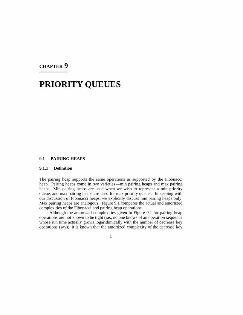
Operation Fibonacci Heap Pairing HeapActual Amortized Actual Amortized

GetMin Ο(1) Ο(1) Ο(1) Ο(1)Insert Ο(1) Ο(1) Ο(1) Ο(1)DeleteMin Ο(n) Ο(log n) Ο(n) Ο(log n)Meld Ο(1) Ο(1) Ο(1) Ο(log n)Delete Ο(n) Ο(log n) Ο(n) Ο(log n)DecreaseKey Ο(n) Ο(1) Ο(1) Ο(log n)

Figure 9.1: Complexity of Fibonacci and pairing heap operations

operation is Ω(loglogn) (see the section titled References and Selected Readingsat the end of this chapter).

Although the amortized complexity is better when a Fibonacci heap is usedrather than when a pairing heap is used, extensive experimental studies employ-ing these structures in the implementation of Dijkstra’s shortest paths algorithm(Section 6.4.1) and Prim’s minimum cost spanning tree algorithm (Section 6.3.2)indicate that pairing heaps actually outperform Fibonacci heaps.

Definition: A min pairing heap is a min tree in which the operations are per-formed in a manner to be specified later.

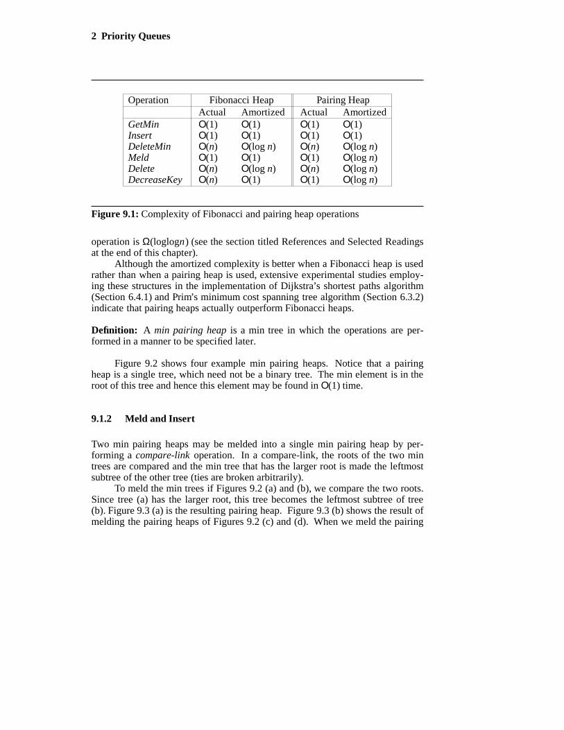
Figure 9.2 shows four example min pairing heaps. Notice that a pairingheap is a single tree, which need not be a binary tree. The min element is in theroot of this tree and hence this element may be found in Ο(1) time.

9.1.2 Meld and Insert

Two min pairing heaps may be melded into a single min pairing heap by per-forming a compare-link operation. In a compare-link, the roots of the two mintrees are compared and the min tree that has the larger root is made the leftmostsubtree of the other tree (ties are broken arbitrarily).

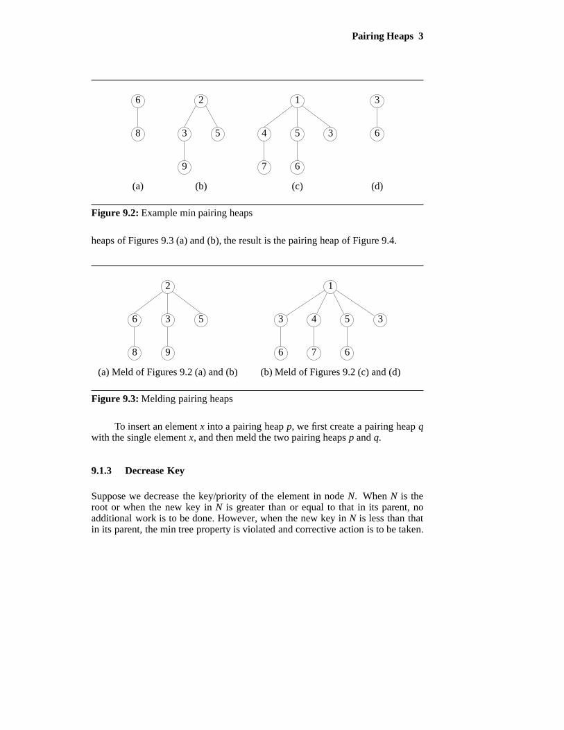
To meld the min trees if Figures 9.2 (a) and (b), we compare the two roots.Since tree (a) has the larger root, this tree becomes the leftmost subtree of tree(b). Figure 9.3 (a) is the resulting pairing heap. Figure 9.3 (b) shows the result ofmelding the pairing heaps of Figures 9.2 (c) and (d). When we meld the pairing

Pairing Heaps 3

8

6

(a)

9

3 5

2

(b)

7

4

6

5 3

1

(c)

6

3

(d)

Figure 9.2: Example min pairing heaps

heaps of Figures 9.3 (a) and (b), the result is the pairing heap of Figure 9.4.

8

6

9

3 5

2

(a) Meld of Figures 9.2 (a) and (b)

6

3

7

4

6

5 3

1

(b) Meld of Figures 9.2 (c) and (d)

Figure 9.3: Melding pairing heaps

To insert an element x into a pairing heap p, we first create a pairing heap qwith the single element x, and then meld the two pairing heaps p and q.

9.1.3 Decrease Key

Suppose we decrease the key/priority of the element in node N. When N is theroot or when the new key in N is greater than or equal to that in its parent, noadditional work is to be done. However, when the new key in N is less than thatin its parent, the min tree property is violated and corrective action is to be taken.

4 Priority Queues

8

6

9

3 5

2

6

3

7

4

6

5 3

1

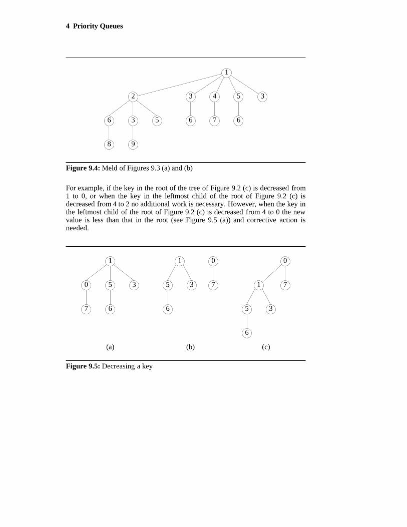
Figure 9.4: Meld of Figures 9.3 (a) and (b)

For example, if the key in the root of the tree of Figure 9.2 (c) is decreased from1 to 0, or when the key in the leftmost child of the root of Figure 9.2 (c) isdecreased from 4 to 2 no additional work is necessary. However, when the key inthe leftmost child of the root of Figure 9.2 (c) is decreased from 4 to 0 the newvalue is less than that in the root (see Figure 9.5 (a)) and corrective action isneeded.

7

0

6

5 3

1

(a)

7

0

6

5 3

1

(b)

7

0

6

5 3

1

(c)

Figure 9.5: Decreasing a key

Pairing Heaps 5

Since pairing heaps are normally not implemented with a parent pointer, itis difficult to determine whether or not corrective action is needed following akey reduction. Therefore, corrective action is taken regardless of whether or notit is needed except when N is the tree root. The corrective action consists of thefollowing steps:

Step 1: Remove the subtree with root N from the tree. This results in two mintrees.

Step 2: Meld the two min trees together.

Figure 9.5 (b) shows the two min trees following Step 1, and Figure 9.5 (c)shows the result following Step 2.

9.1.4 Delete Min

The min element is in the root of the tree. So, to delete the min element, we firstdelete the root node. When the root is deleted, we are left with zero or more mintrees (i.e., the subtrees of the deleted root). When the number of remaining mintrees is two or more, these min trees must be melded into a single min tree. Intwo pass pairing heaps, this melding is done as follows:

Step 1: Make a left to right pass over the trees, melding pairs of trees.

Step 2: Start with the rightmost tree and meld the remaining trees (right to left)into this tree one at a time.

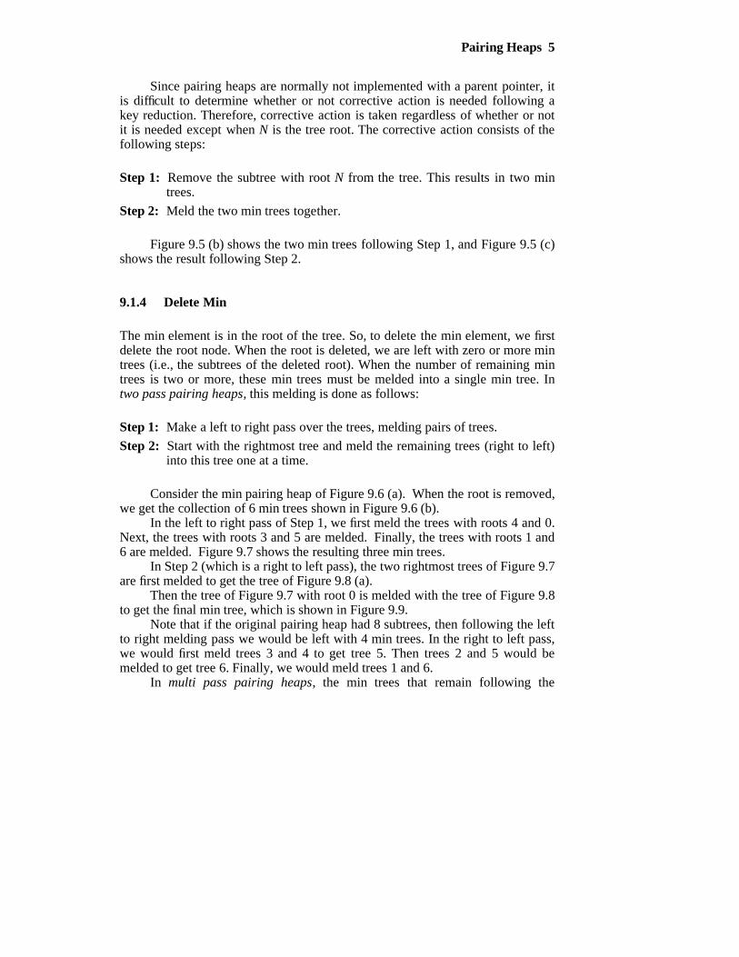
Consider the min pairing heap of Figure 9.6 (a). When the root is removed,we get the collection of 6 min trees shown in Figure 9.6 (b).

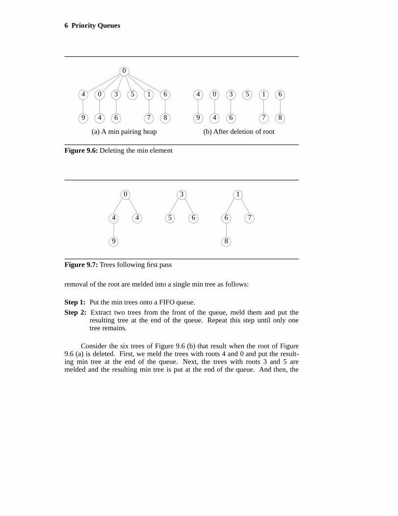
In the left to right pass of Step 1, we first meld the trees with roots 4 and 0.Next, the trees with roots 3 and 5 are melded. Finally, the trees with roots 1 and6 are melded. Figure 9.7 shows the resulting three min trees.

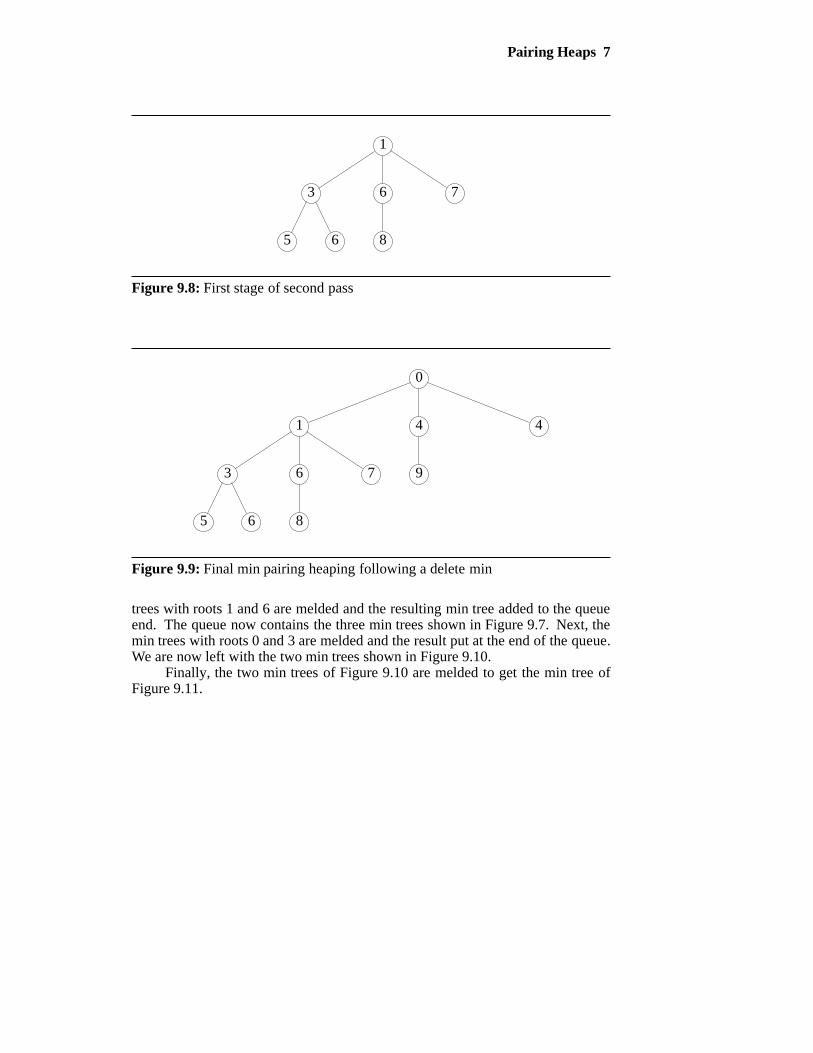
In Step 2 (which is a right to left pass), the two rightmost trees of Figure 9.7are first melded to get the tree of Figure 9.8 (a).

Then the tree of Figure 9.7 with root 0 is melded with the tree of Figure 9.8to get the final min tree, which is shown in Figure 9.9.

Note that if the original pairing heap had 8 subtrees, then following the leftto right melding pass we would be left with 4 min trees. In the right to left pass,we would first meld trees 3 and 4 to get tree 5. Then trees 2 and 5 would bemelded to get tree 6. Finally, we would meld trees 1 and 6.

In multi pass pairing heaps, the min trees that remain following the

6 Priority Queues

9

4

4

0

6

3 5

7

1

8

6

0

(a) A min pairing heap

9

4

4

0

6

3 5

7

1

8

6

(b) After deletion of root

Figure 9.6: Deleting the min element

9

4 4

0

5 6

3

8

6 7

1

Figure 9.7: Trees following first pass

removal of the root are melded into a single min tree as follows:

Step 1: Put the min trees onto a FIFO queue.

Step 2: Extract two trees from the front of the queue, meld them and put theresulting tree at the end of the queue. Repeat this step until only onetree remains.

Consider the six trees of Figure 9.6 (b) that result when the root of Figure9.6 (a) is deleted. First, we meld the trees with roots 4 and 0 and put the result-ing min tree at the end of the queue. Next, the trees with roots 3 and 5 aremelded and the resulting min tree is put at the end of the queue. And then, the

Pairing Heaps 7

5 6

3

8

6 7

1

Figure 9.8: First stage of second pass

5 6

3

8

6 7

1

9

4 4

0

Figure 9.9: Final min pairing heaping following a delete min

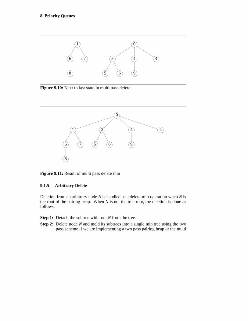
trees with roots 1 and 6 are melded and the resulting min tree added to the queueend. The queue now contains the three min trees shown in Figure 9.7. Next, themin trees with roots 0 and 3 are melded and the result put at the end of the queue.We are now left with the two min trees shown in Figure 9.10.

Finally, the two min trees of Figure 9.10 are melded to get the min tree ofFigure 9.11.

8 Priority Queues

9

4 4

0

5 6

3

8

6 7

1

Figure 9.10: Next to last state in multi pass delete

9

4 4

0

5 6

3

8

6 7

1

Figure 9.11: Result of multi pass delete min

9.1.5 Arbitrary Delete

Deletion from an arbitrary node N is handled as a delete-min operation when N isthe root of the pairing heap. When N is not the tree root, the deletion is done asfollows:

Step 1: Detach the subtree with root N from the tree.

Step 2: Delete node N and meld its subtrees into a single min tree using the twopass scheme if we are implementing a two pass pairing heap or the multi

Pairing Heaps 9

pass scheme if we are implementing a multi pass pairing heap.

Step 3: Meld the min trees from Steps 1 and 2 into a single min tree.

9.1.6 Implementation Considerations

Although we can implement a pairing heap using nodes that have a variablenumber of children fields, such an implementation is expensive because of theneed to dynamically increase the number of children fields as needed. Anefficient implementation results when we use the binary tree representation of atree (see Section 5.1.2.2). Siblings in the original min tree are linked togetherusing a doubly linked list. In addition to a data field, each node has the threepointer fields previous, next, and child. The leftmost node in a doubly linked listof siblings uses its previous pointer to point to its parent. A leftmost childsatisfies the property x → previous → child = x. The doubly linked list makes itis possible to remove an arbitrary element (as is required by the Delete andDecreaseKey operations) in Ο(1) time.

9.1.7 Complexity

You can verify that using the described binary tree representation, all pairingheap operations (other than Delete and DeleteMin) can be done in Ο(1) time.The complexity of the Delete and DeleteMin operations is Ο(n), because thenumber of subtrees that have to be melded following the removal of a node isΟ(n).

The amortized complexity of the pairing heap operations is established inthe paper by Fredman et al. cited in the References and Selected Readings sec-tion. Experimental studies conducted by Stasko and Vitter (see their paper thatis cited in the References and Selected Readings section) establish the superior-ity of two pass pairing heaps over multipass pairing heaps.

EXERCISES

1. (a) Into an empty two pass min pairing heap, insert elements with priori-ties 20, 10, 5, 18, 6, 12, 14, 9, 8 and 22 (in this order). Show the minpairing heap following each insert.

(b) Delete the min element from the final min pairing heap of part (a).Show the resulting pairing heap.

10 Priority Queues

2. (a) Into an empty multi pass min pairing heap, insert elements withpriorities 20, 10, 5, 18, 6, 12, 14, 9, 8 and 22 (in this order). Show themin pairing heap following each insert.

(b) Delete the min element from the final min pairing heap of part (a).Show the resulting pairing heap.

3. Fully code and test the class MultiPassPairingHeap, which impements amulti pass min pairing heap. Your class must include the functions Get-Min, Insert, DeleteMin , Meld, Delete and DecreaseKey . The functionInsert should return the node into which the new element was inserted.This returned information can later be used as an input to Delete andDecreaseKey .

4. What are the worst-case height and degree of a pairing heap that has n ele-ments? Show how you arrived at your answer.

5. Define a one pass pairing heap as an adaptation of a two pass pairing heapin which Step 1 (Make a left to right pass over the trees, melding pairs oftrees.) is eliminated. Show that the amortized cost of either insert or deletemin must be Θ(n).

9.2 SYMMETRIC MIN-MAX HEAPS

9.2.1 Definition and Properties

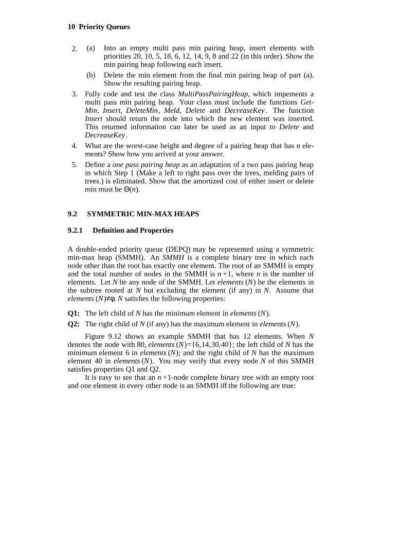
A double-ended priority queue (DEPQ) may be represented using a symmetricmin-max heap (SMMH). An SMMH is a complete binary tree in which eachnode other than the root has exactly one element. The root of an SMMH is emptyand the total number of nodes in the SMMH is n +1, where n is the number ofelements. Let N be any node of the SMMH. Let elements (N) be the elements inthe subtree rooted at N but excluding the element (if any) in N. Assume thatelements (N)≠φ. N satisfies the following properties:

Q1: The left child of N has the minimum element in elements (N).

Q2: The right child of N (if any) has the maximum element in elements (N).

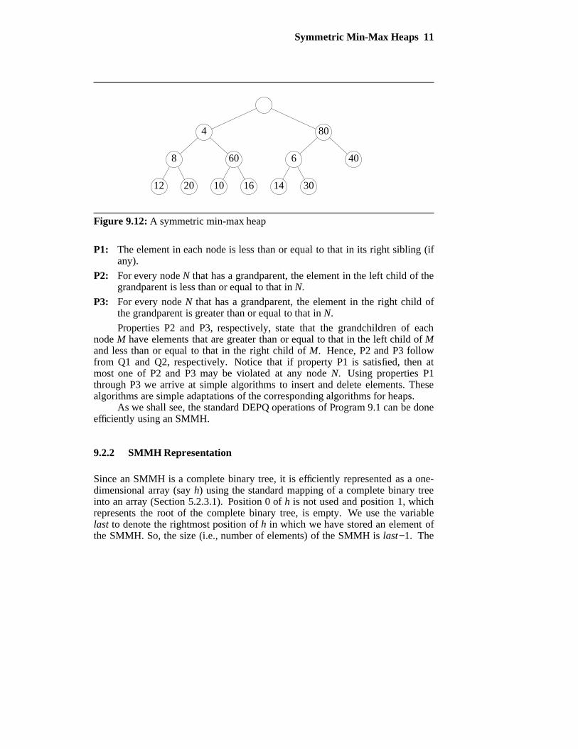
Figure 9.12 shows an example SMMH that has 12 elements. When Ndenotes the node with 80, elements (N)=6,14,30,40; the left child of N has theminimum element 6 in elements (N); and the right child of N has the maximumelement 40 in elements (N). You may verify that every node N of this SMMHsatisfies properties Q1 and Q2.

It is easy to see that an n +1-node complete binary tree with an empty rootand one element in every other node is an SMMH iff the following are true:

Symmetric Min-Max Heaps 11

12 20 10 16 14 30

8 60 6 40

4 80

Figure 9.12: A symmetric min-max heap

P1: The element in each node is less than or equal to that in its right sibling (ifany).

P2: For every node N that has a grandparent, the element in the left child of thegrandparent is less than or equal to that in N.

P3: For every node N that has a grandparent, the element in the right child ofthe grandparent is greater than or equal to that in N.

Properties P2 and P3, respectively, state that the grandchildren of eachnode M have elements that are greater than or equal to that in the left child of Mand less than or equal to that in the right child of M. Hence, P2 and P3 followfrom Q1 and Q2, respectively. Notice that if property P1 is satisfied, then atmost one of P2 and P3 may be violated at any node N. Using properties P1through P3 we arrive at simple algorithms to insert and delete elements. Thesealgorithms are simple adaptations of the corresponding algorithms for heaps.

As we shall see, the standard DEPQ operations of Program 9.1 can be doneefficiently using an SMMH.

9.2.2 SMMH Representation

Since an SMMH is a complete binary tree, it is efficiently represented as a one-dimensional array (say h) using the standard mapping of a complete binary treeinto an array (Section 5.2.3.1). Position 0 of h is not used and position 1, whichrepresents the root of the complete binary tree, is empty. We use the variablelast to denote the rightmost position of h in which we have stored an element ofthe SMMH. So, the size (i.e., number of elements) of the SMMH is last−1. The

12 Priority Queues

variable arrayLength keeps track of the current number of positions in the arrayh.

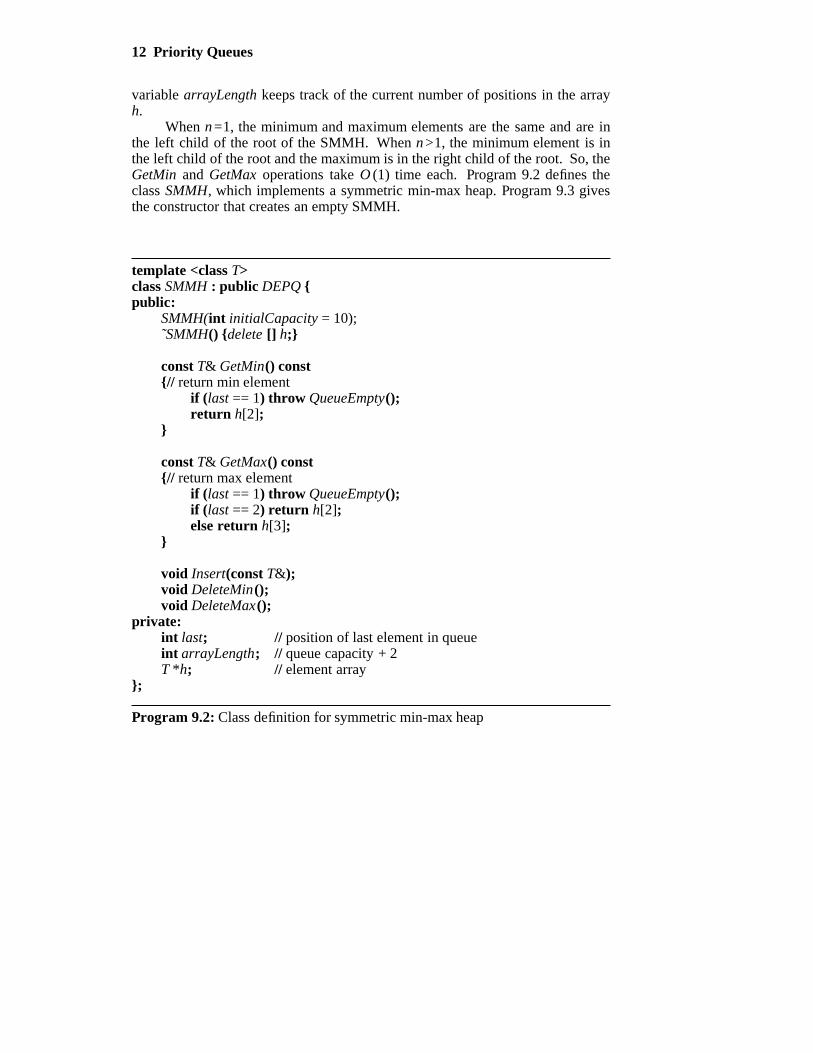
When n=1, the minimum and maximum elements are the same and are inthe left child of the root of the SMMH. When n>1, the minimum element is inthe left child of the root and the maximum is in the right child of the root. So, theGetMin and GetMax operations take O (1) time each. Program 9.2 defines theclass SMMH, which implements a symmetric min-max heap. Program 9.3 givesthe constructor that creates an empty SMMH.

template <class T>class SMMH : public DEPQ public:

SMMH(int initialCapacity = 10);˜SMMH() delete [] h;

const T& GetMin() const// return min element

if (last == 1) throw QueueEmpty();return h[2];

const T& GetMax() const// return max element

if (last == 1) throw QueueEmpty();if (last == 2) return h[2];else return h[3];

void Insert(const T&);void DeleteMin();void DeleteMax();

private:int last; // position of last element in queueint arrayLength; // queue capacity + 2T *h; // element array

;

Program 9.2: Class definition for symmetric min-max heap


template <class T>SMMH<T>::SMMH(int initialCapacity)// Constructor.

if (initialCapacity < 1)

ostringstream s;s << "Initial capacity = " << initialCapacity << " Must be > 0";throw IllegalParameterValue(s.str());

arrayLength = initialCapacity + 2;h = new T[arrayLength];last = 1;

Program 9.3 Constructor for SMMH

9.2.3 Inserting into an SMMH

The algorithm to insert into an SMMH has three steps.

Step 1: Expand the size of the complete binary tree by 1, creating a new node Efor the element x that is to be inserted. This newly created node of thecomplete binary tree becomes the candidate node to insert the new ele-ment x.

Step 2: Verify whether the insertion of x into E would result in a violation ofproperty P1. Note that this violation occurs iff E is a right child of itsparent and x is greater than the element in the sibling of E. In case of aP1 violation, the element in the sibling of E is moved to E and E isupdated to be the now empty sibling.

Step 3: Perform a bubble-up pass from E up the tree verifying properties P2 andP3. In each round of the bubble-up pass, E moves up the tree by onelevel. When E is positioned so that the insertion of x into E doesn’tresult in a violation of either P2 or P3, insert x into E.

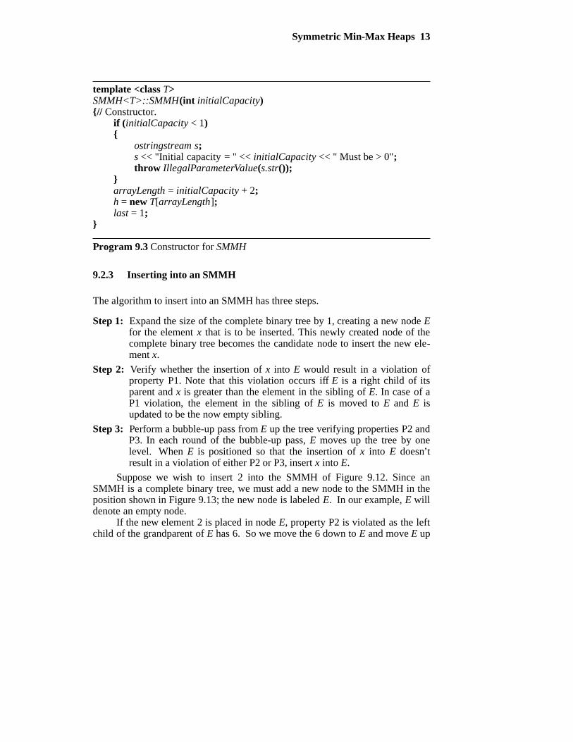
Suppose we wish to insert 2 into the SMMH of Figure 9.12. Since anSMMH is a complete binary tree, we must add a new node to the SMMH in theposition shown in Figure 9.13; the new node is labeled E. In our example, E willdenote an empty node.

If the new element 2 is placed in node E, property P2 is violated as the leftchild of the grandparent of E has 6. So we move the 6 down to E and move E up

14 Priority Queues

12 20 10 16 14 30 E

8 60 6 40

4 80

Figure 9.13: The SMMH of Figure 9.12 with a node added

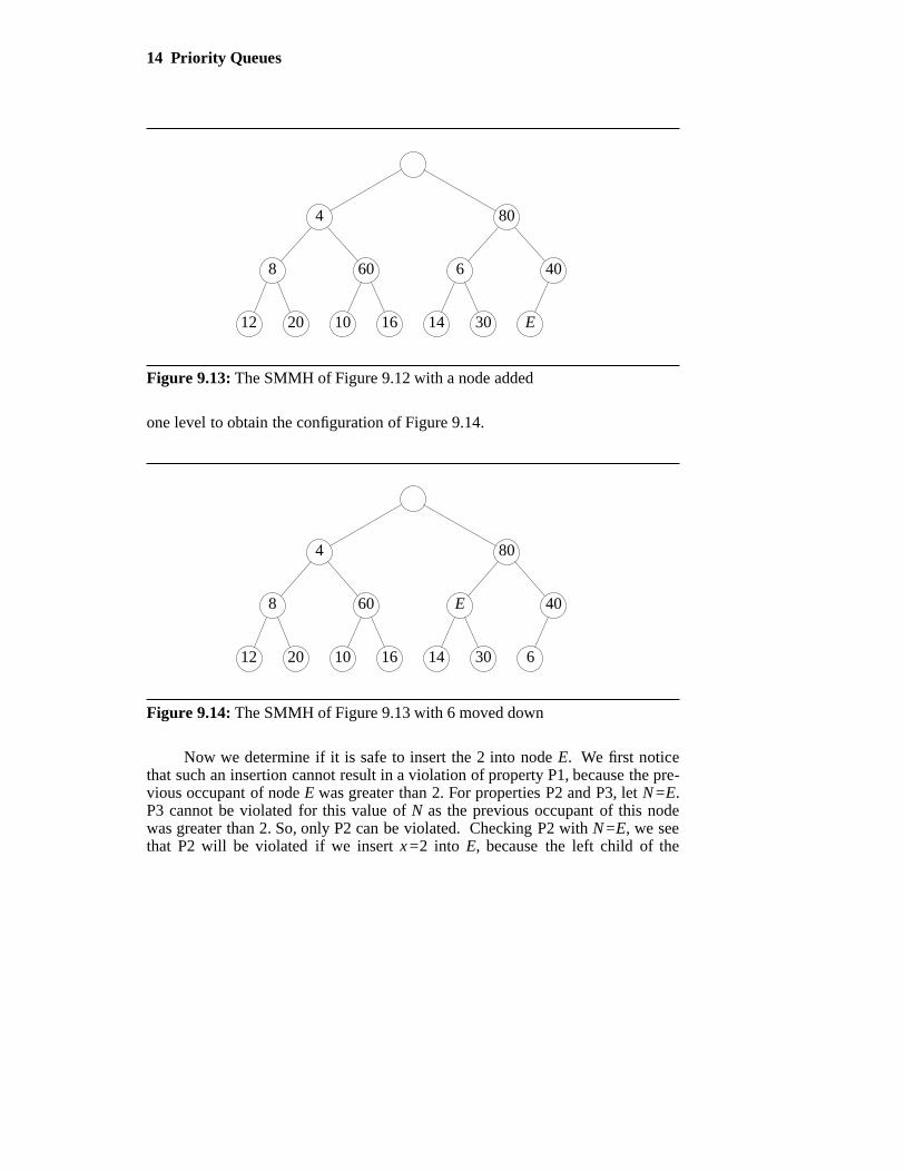
one level to obtain the configuration of Figure 9.14.

12 20 10 16 14 30 6

8 60 E 40

4 80

Figure 9.14: The SMMH of Figure 9.13 with 6 moved down

Now we determine if it is safe to insert the 2 into node E. We first noticethat such an insertion cannot result in a violation of property P1, because the pre-vious occupant of node E was greater than 2. For properties P2 and P3, let N=E.P3 cannot be violated for this value of N as the previous occupant of this nodewas greater than 2. So, only P2 can be violated. Checking P2 with N=E, we seethat P2 will be violated if we insert x=2 into E, because the left child of the


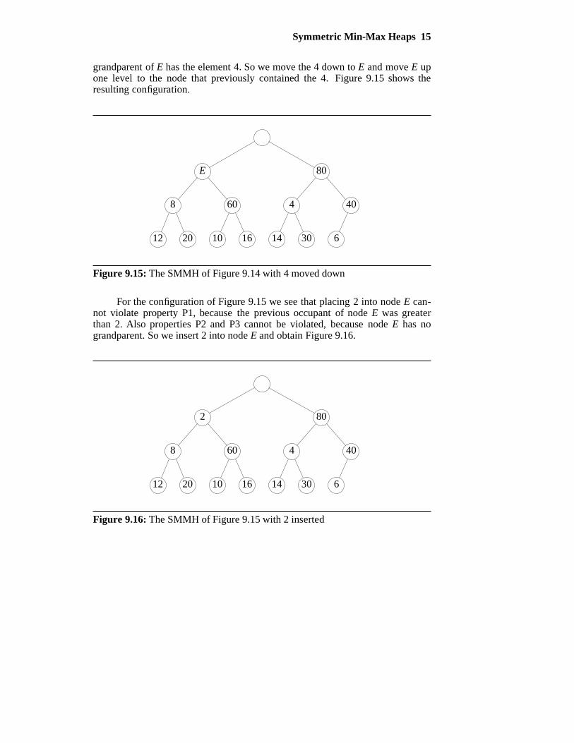
grandparent of E has the element 4. So we move the 4 down to E and move E upone level to the node that previously contained the 4. Figure 9.15 shows theresulting configuration.

12 20 10 16 14 30 6

8 60 4 40

E 80


For the configuration of Figure 9.15 we see that placing 2 into node E can-not violate property P1, because the previous occupant of node E was greaterthan 2. Also properties P2 and P3 cannot be violated, because node E has nograndparent. So we insert 2 into node E and obtain Figure 9.16.

12 20 10 16 14 30 6

8 60 4 40

2 80

Figure 9.16: The SMMH of Figure 9.15 with 2 inserted

16 Priority Queues

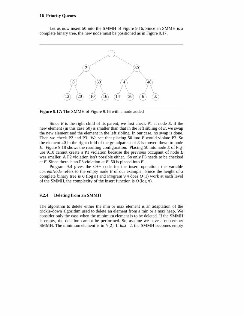
Let us now insert 50 into the SMMH of Figure 9.16. Since an SMMH is acomplete binary tree, the new node must be positioned as in Figure 9.17.

12 20 10 16 14 30 6 E

8 60 4 40

2 80

Figure 9.17: The SMMH of Figure 9.16 with a node added

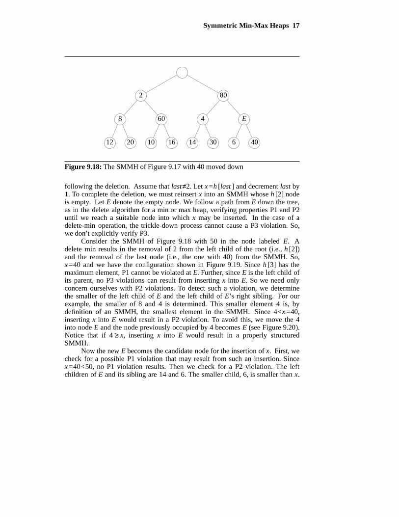
Since E is the right child of its parent, we first check P1 at node E. If thenew element (in this case 50) is smaller than that in the left sibling of E, we swapthe new element and the element in the left sibling. In our case, no swap is done.Then we check P2 and P3. We see that placing 50 into E would violate P3. Sothe element 40 in the right child of the grandparent of E is moved down to nodeE. Figure 9.18 shows the resulting configuration. Placing 50 into node E of Fig-ure 9.18 cannot create a P1 violation because the previous occupant of node Ewas smaller. A P2 violation isn’t possible either. So only P3 needs to be checkedat E. Since there is no P3 violation at E, 50 is placed into E.

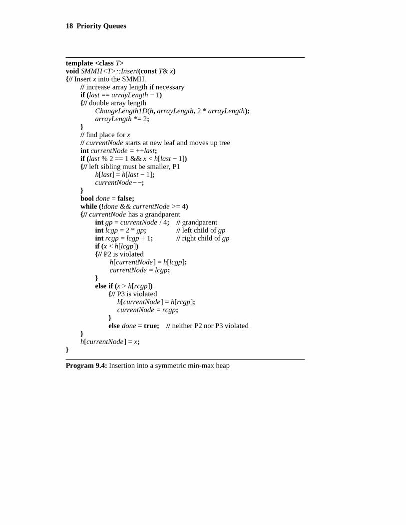
Program 9.4 gives the C++ code for the insert operation; the variablecurrentNode refers to the empty node E of our example. Since the height of acomplete binary tree is O (log n) and Program 9.4 does O (1) work at each levelof the SMMH, the complexity of the insert function is O (log n).

9.2.4 Deleting from an SMMH

The algorithm to delete either the min or max element is an adaptation of thetrickle-down algorithm used to delete an element from a min or a max heap. Weconsider only the case when the minimum element is to be deleted. If the SMMHis empty, the deletion cannot be performed. So, assume we have a non-emptySMMH. The minimum element is in h [2]. If last=2, the SMMH becomes empty


12 20 10 16 14 30 6 40

8 60 4 E

2 80


following the deletion. Assume that last≠2. Let x=h [last ] and decrement last by1. To complete the deletion, we must reinsert x into an SMMH whose h [2] nodeis empty. Let E denote the empty node. We follow a path from E down the tree,as in the delete algorithm for a min or max heap, verifying properties P1 and P2until we reach a suitable node into which x may be inserted. In the case of adelete-min operation, the trickle-down process cannot cause a P3 violation. So,we don’t explicitly verify P3.

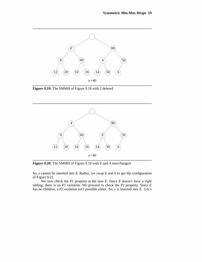
Consider the SMMH of Figure 9.18 with 50 in the node labeled E. Adelete min results in the removal of 2 from the left child of the root (i.e., h [2])and the removal of the last node (i.e., the one with 40) from the SMMH. So,x=40 and we have the configuration shown in Figure 9.19. Since h [3] has themaximum element, P1 cannot be violated at E. Further, since E is the left child ofits parent, no P3 violations can result from inserting x into E. So we need onlyconcern ourselves with P2 violations. To detect such a violation, we determinethe smaller of the left child of E and the left child of E’s right sibling. For ourexample, the smaller of 8 and 4 is determined. This smaller element 4 is, bydefinition of an SMMH, the smallest element in the SMMH. Since 4<x=40,inserting x into E would result in a P2 violation. To avoid this, we move the 4into node E and the node previously occupied by 4 becomes E (see Figure 9.20).Notice that if 4 ≥ x, inserting x into E would result in a properly structuredSMMH.

Now the new E becomes the candidate node for the insertion of x. First, wecheck for a possible P1 violation that may result from such an insertion. Sincex=40<50, no P1 violation results. Then we check for a P2 violation. The leftchildren of E and its sibling are 14 and 6. The smaller child, 6, is smaller than x.

18 Priority Queues

template <class T>void SMMH<T>::Insert(const T& x)// Insert x into the SMMH.

// increase array length if necessaryif (last == arrayLength − 1)// double array length

ChangeLength1D(h, arrayLength, 2 * arrayLength);arrayLength *= 2;

// find place for x// currentNode starts at new leaf and moves up treeint currentNode = ++last;if (last % 2 == 1 && x < h[last − 1])// left sibling must be smaller, P1

h[last] = h[last − 1];currentNode− −;

bool done = false;while (!done && currentNode >= 4)// currentNode has a grandparent

int gp = currentNode / 4; // grandparentint lcgp = 2 * gp; // left child of gpint rcgp = lcgp + 1; // right child of gpif (x < h[lcgp])// P2 is violated

h[currentNode] = h[lcgp];currentNode = lcgp;

else if (x > h[rcgp])

// P3 is violatedh[currentNode] = h[rcgp];currentNode = rcgp;

else done = true; // neither P2 nor P3 violated

h[currentNode] = x;

Program 9.4: Insertion into a symmetric min-max heap


12 20 10 16 14 30 6

8 60 4 50

E 80

x=40

Figure 9.19: The SMMH of Figure 9.18 with 2 deleted

12 20 10 16 14 30 6

8 60 E 50

4 80

x=40

Figure 9.20: The SMMH of Figure 9.19 with E and 4 interchanged

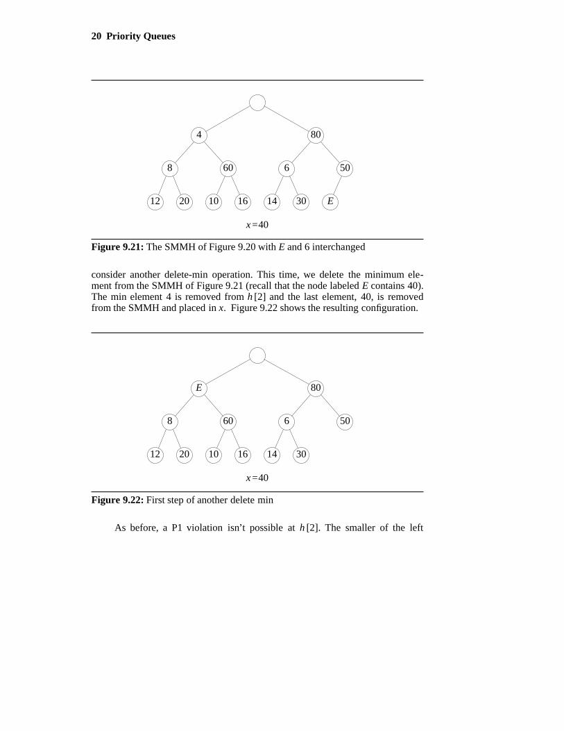
So, x cannot be inserted into E. Rather, we swap E and 6 to get the configurationof Figure 9.21.

We now check the P1 property at the new E. Since E doesn’t have a rightsibling, there is no P1 violation. We proceed to check the P2 property. Since Ehas no children, a P2 violation isn’t possible either. So, x is inserted into E. Let’s

20 Priority Queues

12 20 10 16 14 30 E

8 60 6 50

4 80

x=40


consider another delete-min operation. This time, we delete the minimum ele-ment from the SMMH of Figure 9.21 (recall that the node labeled E contains 40).The min element 4 is removed from h [2] and the last element, 40, is removedfrom the SMMH and placed in x. Figure 9.22 shows the resulting configuration.

12 20 10 16 14 30

8 60 6 50

E 80

x=40

Figure 9.22: First step of another delete min

As before, a P1 violation isn’t possible at h [2]. The smaller of the left


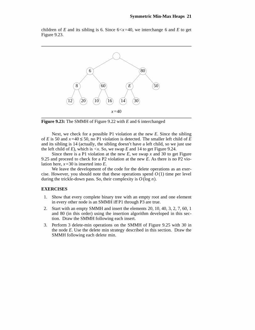
children of E and its sibling is 6. Since 6<x=40, we interchange 6 and E to getFigure 9.23.

12 20 10 16 14 30

8 60 E 50

6 80

x=40


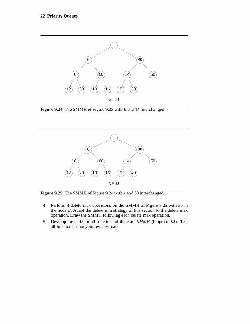
Next, we check for a possible P1 violation at the new E. Since the siblingof E is 50 and x=40 ≤ 50, no P1 violation is detected. The smaller left child of Eand its sibling is 14 (actually, the sibling doesn’t have a left child, so we just usethe left child of E), which is <x. So, we swap E and 14 to get Figure 9.24.

Since there is a P1 violation at the new E, we swap x and 30 to get Figure9.25 and proceed to check for a P2 violation at the new E. As there is no P2 vio-lation here, x=30 is inserted into E.

We leave the development of the code for the delete operations as an exer-cise. However, you should note that these operations spend O (1) time per levelduring the trickle-down pass. So, their complexity is O (log n).

EXERCISES

1. Show that every complete binary tree with an empty root and one elementin every other node is an SMMH iff P1 through P3 are true.

2. Start with an empty SMMH and insert the elements 20, 10, 40, 3, 2, 7, 60, 1and 80 (in this order) using the insertion algorithm developed in this sec-tion. Draw the SMMH following each insert.

3. Perform 3 delete-min operations on the SMMH of Figure 9.25 with 30 inthe node E. Use the delete min strategy described in this section. Draw theSMMH following each delete min.

22 Priority Queues

12 20 10 16 E 30

8 60 14 50

6 80

x=40


12 20 10 16 E 40

8 60 14 50

6 80

x=30

Figure 9.25: The SMMH of Figure 9.24 with x and 30 interchanged

4. Perform 4 delete max operations on the SMMH of Figure 9.25 with 30 inthe node E. Adapt the delete min strategy of this section to the delete maxoperation. Draw the SMMH following each delete max operation.

5. Develop the code for all functions of the class SMMH (Program 9.2). Testall functions using your own test data.

Interval Heaps 23

9.3 INTERVAL HEAPS

9.3.1 Definition and Properties

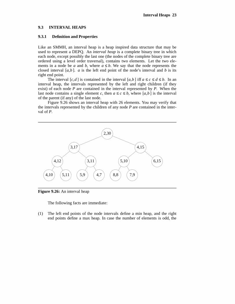
Like an SMMH, an interval heap is a heap inspired data structure that may beused to represent a DEPQ. An interval heap is a complete binary tree in whicheach node, except possibly the last one (the nodes of the complete binary tree areordered using a level order traversal), contains two elements. Let the two ele-ments in a node be a and b, where a ≤ b. We say that the node represents theclosed interval [a,b ]. a is the left end point of the node’s interval and b is itsright end point.

The interval [c,d ] is contained in the interval [a,b ] iff a ≤ c ≤ d ≤ b. In aninterval heap, the intervals represented by the left and right children (if theyexist) of each node P are contained in the interval represented by P. When thelast node contains a single element c, then a ≤ c ≤ b, where [a,b ] is the intervalof the parent (if any) of the last node.

Figure 9.26 shows an interval heap with 26 elements. You may verify thatthe intervals represented by the children of any node P are contained in the inter-val of P.

4,10 5,11 5,9 4,7 8,8 7,9

4,12 3,11 5,10 6,15

3,17 4,15

2,30

Figure 9.26: An interval heap

The following facts are immediate:

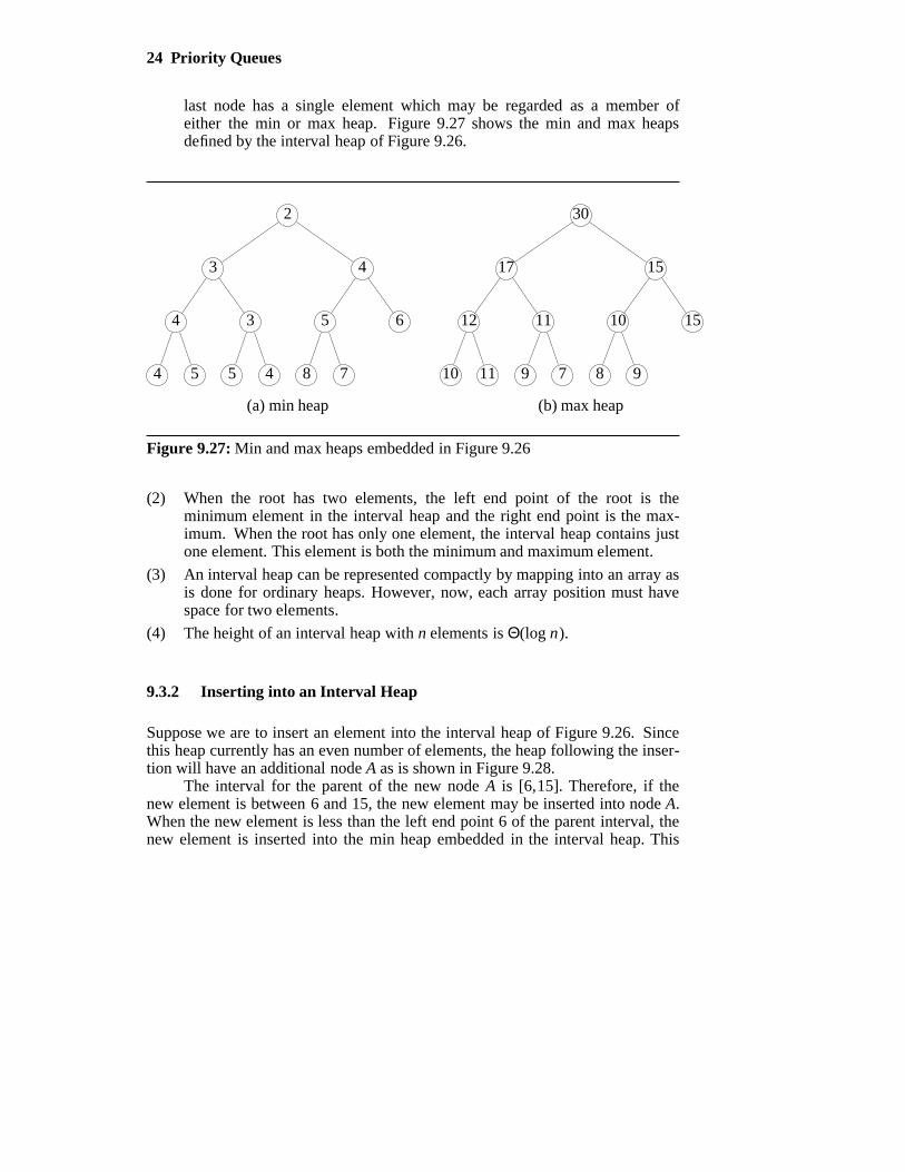
(1) The left end points of the node intervals define a min heap, and the rightend points define a max heap. In case the number of elements is odd, the

24 Priority Queues

last node has a single element which may be regarded as a member ofeither the min or max heap. Figure 9.27 shows the min and max heapsdefined by the interval heap of Figure 9.26.

4 5 5 4 8 7

4 3 5 6

3 4

2

(a) min heap

10 11 9 7 8 9

12 11 10 15

17 15

30

(b) max heap

Figure 9.27: Min and max heaps embedded in Figure 9.26

(2) When the root has two elements, the left end point of the root is theminimum element in the interval heap and the right end point is the max-imum. When the root has only one element, the interval heap contains justone element. This element is both the minimum and maximum element.

(3) An interval heap can be represented compactly by mapping into an array asis done for ordinary heaps. However, now, each array position must havespace for two elements.

(4) The height of an interval heap with n elements is Θ(log n).

9.3.2 Inserting into an Interval Heap

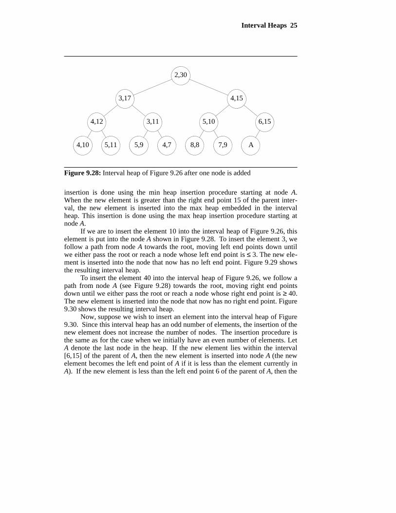
Suppose we are to insert an element into the interval heap of Figure 9.26. Sincethis heap currently has an even number of elements, the heap following the inser-tion will have an additional node A as is shown in Figure 9.28.

The interval for the parent of the new node A is [6,15]. Therefore, if thenew element is between 6 and 15, the new element may be inserted into node A.When the new element is less than the left end point 6 of the parent interval, thenew element is inserted into the min heap embedded in the interval heap. This

Interval Heaps 25

4,10 5,11 5,9 4,7 8,8 7,9 A

4,12 3,11 5,10 6,15

3,17 4,15

2,30

Figure 9.28: Interval heap of Figure 9.26 after one node is added

insertion is done using the min heap insertion procedure starting at node A.When the new element is greater than the right end point 15 of the parent inter-val, the new element is inserted into the max heap embedded in the intervalheap. This insertion is done using the max heap insertion procedure starting atnode A.

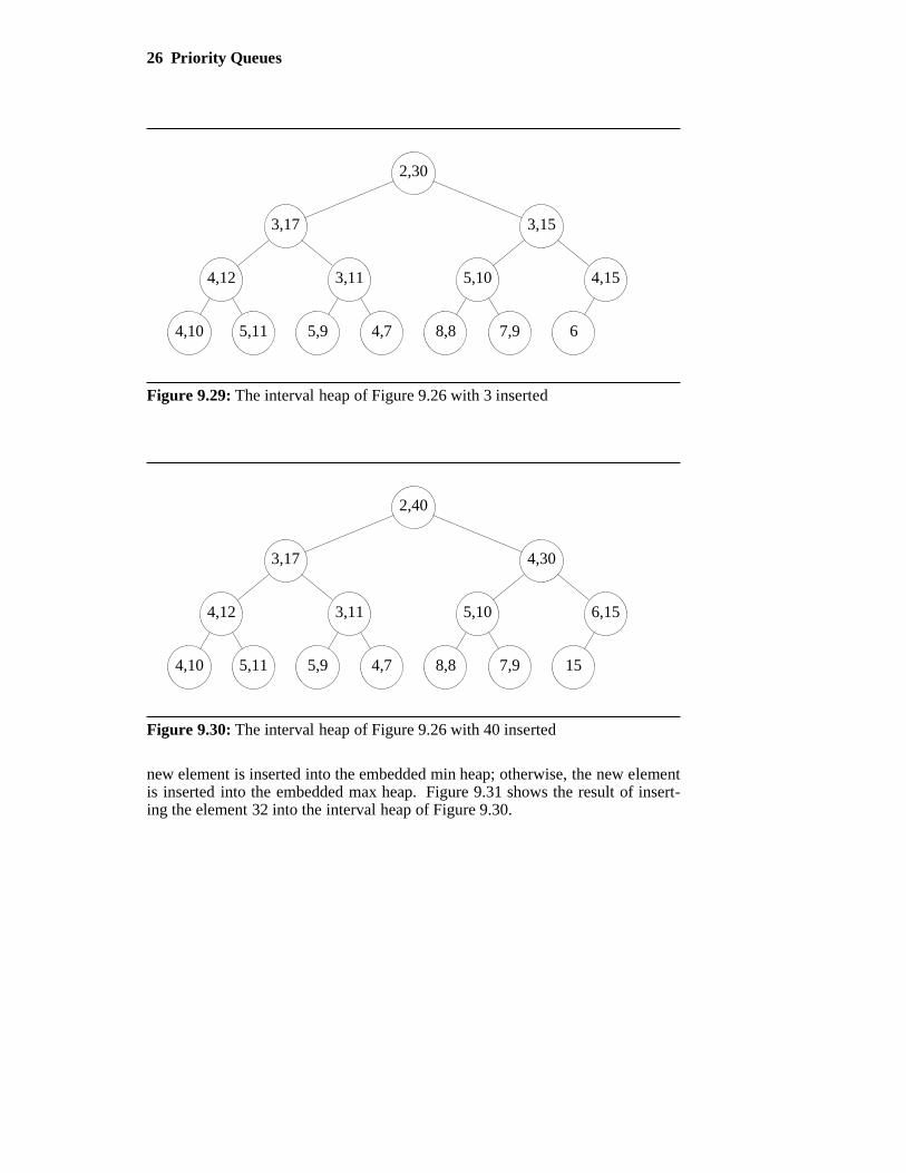
If we are to insert the element 10 into the interval heap of Figure 9.26, thiselement is put into the node A shown in Figure 9.28. To insert the element 3, wefollow a path from node A towards the root, moving left end points down untilwe either pass the root or reach a node whose left end point is ≤ 3. The new ele-ment is inserted into the node that now has no left end point. Figure 9.29 showsthe resulting interval heap.

To insert the element 40 into the interval heap of Figure 9.26, we follow apath from node A (see Figure 9.28) towards the root, moving right end pointsdown until we either pass the root or reach a node whose right end point is ≥ 40.The new element is inserted into the node that now has no right end point. Figure9.30 shows the resulting interval heap.

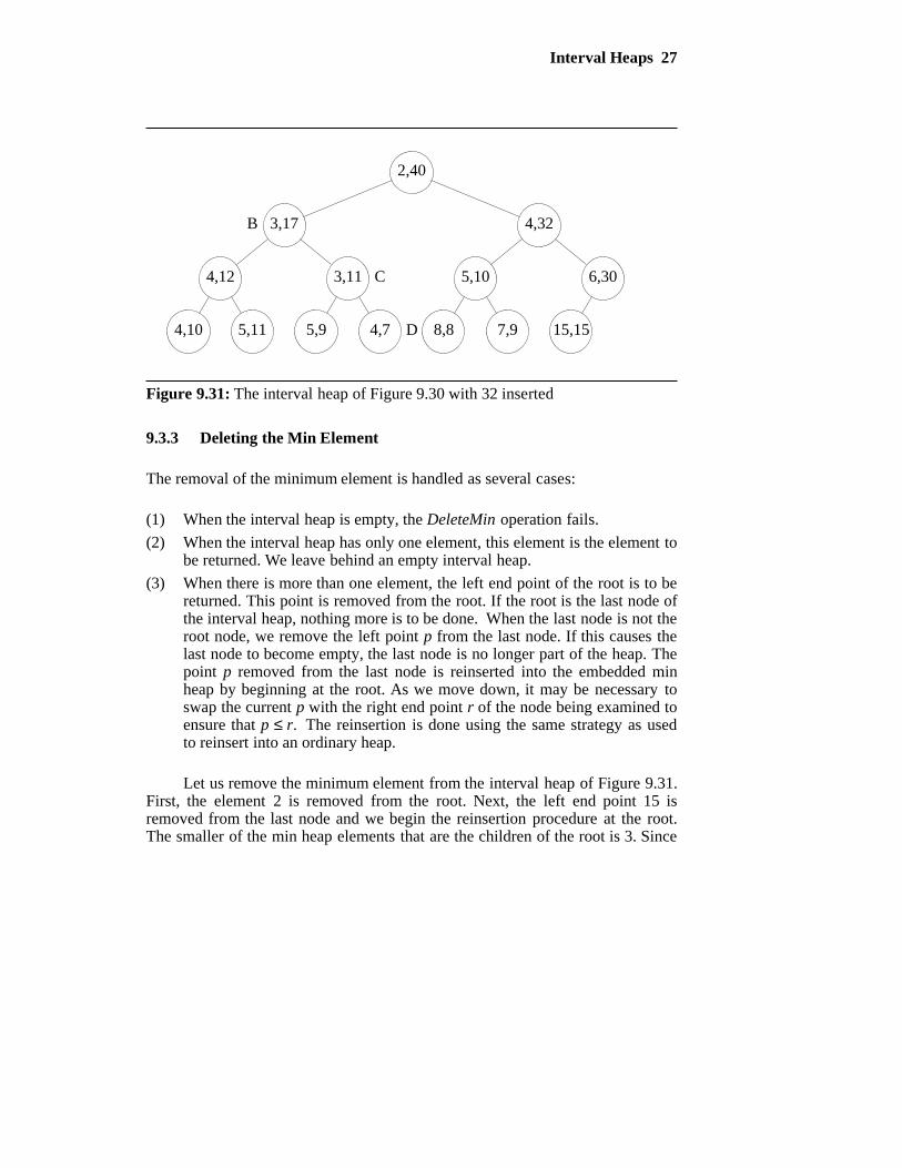
Now, suppose we wish to insert an element into the interval heap of Figure9.30. Since this interval heap has an odd number of elements, the insertion of thenew element does not increase the number of nodes. The insertion procedure isthe same as for the case when we initially have an even number of elements. LetA denote the last node in the heap. If the new element lies within the interval[6,15] of the parent of A, then the new element is inserted into node A (the newelement becomes the left end point of A if it is less than the element currently inA). If the new element is less than the left end point 6 of the parent of A, then the

26 Priority Queues

4,10 5,11 5,9 4,7 8,8 7,9 6

4,12 3,11 5,10 4,15

3,17 3,15

2,30

Figure 9.29: The interval heap of Figure 9.26 with 3 inserted

4,10 5,11 5,9 4,7 8,8 7,9 15

4,12 3,11 5,10 6,15

3,17 4,30

2,40


new element is inserted into the embedded min heap; otherwise, the new elementis inserted into the embedded max heap. Figure 9.31 shows the result of insert-ing the element 32 into the interval heap of Figure 9.30.

Interval Heaps 27

4,10 5,11 5,9 4,7 8,8 7,9 15,15

4,12 3,11 5,10 6,30

3,17 4,32

2,40

D

C

B


9.3.3 Deleting the Min Element

The removal of the minimum element is handled as several cases:

(1) When the interval heap is empty, the DeleteMin operation fails.

(2) When the interval heap has only one element, this element is the element tobe returned. We leave behind an empty interval heap.

(3) When there is more than one element, the left end point of the root is to bereturned. This point is removed from the root. If the root is the last node ofthe interval heap, nothing more is to be done. When the last node is not theroot node, we remove the left point p from the last node. If this causes thelast node to become empty, the last node is no longer part of the heap. Thepoint p removed from the last node is reinserted into the embedded minheap by beginning at the root. As we move down, it may be necessary toswap the current p with the right end point r of the node being examined toensure that p ≤ r. The reinsertion is done using the same strategy as usedto reinsert into an ordinary heap.

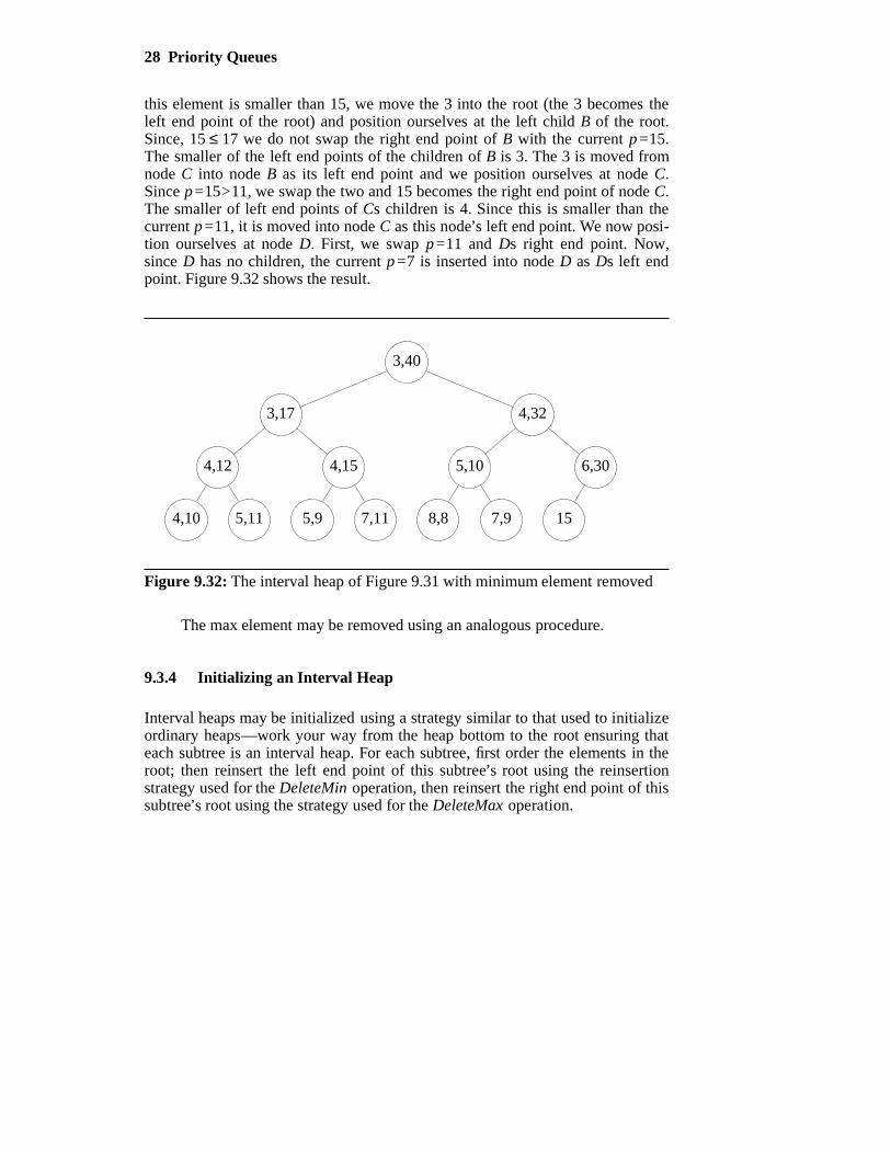
Let us remove the minimum element from the interval heap of Figure 9.31.First, the element 2 is removed from the root. Next, the left end point 15 isremoved from the last node and we begin the reinsertion procedure at the root.The smaller of the min heap elements that are the children of the root is 3. Since

28 Priority Queues

this element is smaller than 15, we move the 3 into the root (the 3 becomes theleft end point of the root) and position ourselves at the left child B of the root.Since, 15 ≤ 17 we do not swap the right end point of B with the current p=15.The smaller of the left end points of the children of B is 3. The 3 is moved fromnode C into node B as its left end point and we position ourselves at node C.Since p=15>11, we swap the two and 15 becomes the right end point of node C.The smaller of left end points of Cs children is 4. Since this is smaller than thecurrent p=11, it is moved into node C as this node’s left end point. We now posi-tion ourselves at node D. First, we swap p=11 and Ds right end point. Now,since D has no children, the current p=7 is inserted into node D as Ds left endpoint. Figure 9.32 shows the result.

4,10 5,11 5,9 7,11 8,8 7,9 15

4,12 4,15 5,10 6,30

3,17 4,32

3,40

Figure 9.32: The interval heap of Figure 9.31 with minimum element removed

The max element may be removed using an analogous procedure.

9.3.4 Initializing an Interval Heap

Interval heaps may be initialized using a strategy similar to that used to initializeordinary heaps—work your way from the heap bottom to the root ensuring thateach subtree is an interval heap. For each subtree, first order the elements in theroot; then reinsert the left end point of this subtree’s root using the reinsertionstrategy used for the DeleteMin operation, then reinsert the right end point of thissubtree’s root using the strategy used for the DeleteMax operation.

Interval Heaps 29

9.3.5 Complexity of Interval Heap Operations

The operations GetMin () and GetMax () take Ο(1) time each; Insert (x), Delete-Min (), and DeleteMax () take Ο(log n) each; and initializing an n element inter-val heap takes Θ(n) time.

9.3.6 The Complementary Range Search Problem

In the complementary range search problem, we have a dynamic collection (i.e.,points are added and removed from the collection as time goes on) of one-dimensional points (i.e., points have only an x-coordinate associated with them)and we are to answer queries of the form: what are the points outside of the inter-val [a,b ]? For example, if the point collection is 3,4,5,6,8,12, the points outsidethe range [5,7] are 3,4,8,12.

When an interval heap is used to represent the point collection, a new pointcan be inserted or an old one removed in Ο(log n) time, where n is the number ofpoints in the collection. Note that given the location of an arbitrary element inan interval heap, this element can be removed from the interval heap in Ο(log n)time using an algorithm similar to that used to remove an arbitrary element froma heap.

The complementary range query can be answered in Θ(k) time, where k isthe number of points outside the range [a,b ]. This is done using the followingrecursive procedure:

Step 1: If the interval tree is empty, return.

Step 2: If the root interval is contained in [a,b ], then all points are in the range(therefore, there are no points to report), return.

Step 3: Report the end points of the root interval that are not in the range [a,b ].

Step 4: Recursively search the left subtree of the root for additional points thatare not in the range [a,b ].

Step 5: Recursively search the right subtree of the root for additional points thatare not in the range [a,b ].

Step 6: return.

Let us try this procedure on the interval heap of Figure 9.31. The queryinterval is [4,32]. We start at the root. Since the root interval is not contained inthe query interval, we reach step 3 of the procedure. Whenever step 3 is reached,we are assured that at least one of the end points of the root interval is outsidethe query interval. Therefore, each time step 3 is reached, at least one point is

30 Priority Queues

reported. In our example, both points 2 and 40 are outside the query interval andare reported. We then search the left and right subtrees of the root for additionalpoints. When the left subtree is searched, we again determine that the root inter-val is not contained in the query interval. This time only one of the root intervalpoints (i.e., 3) is outside the query range. This point is reported and we proceedto search the left and right subtrees of B for additional points outside the queryrange. Since the interval of the left child of B is contained in the query range, theleft subtree of B contains no points outside the query range. We do not explorethe left subtree of B further. When the right subtree of B is searched, we reportthe left end point 3 of node C and proceed to search the left and right subtrees ofC. Since the intervals of the roots of each of these subtrees is contained in thequery interval, these subtrees are not explored further. Finally, we examine theroot of the right subtree of the overall tree root, that is the node with interval[4,32]. Since this node’s interval is contained in the query interval, the right sub-tree of the overall tree is not searched further.

We say that a node is visited if its interval is examined in Step 2. With thisdefinition of visited, we see that the complexity of the above six step procedureis Θ(number of nodes visited). The nodes visited in the preceding example arethe root and its two children, the two children of node B, and the two children ofnode C. So, 7 nodes are visited and a total of 4 points are reported.

We show that the total number of interval heap nodes visited is at most3k+1, where k is the number of points reported. If a visited node reports one ortwo points, give the node a count of one. If a visited node reports no points, giveit a count of zero and add one to the count of its parent (unless the node is theroot and so has no parent). The number of nodes with a nonzero count is at mostk. Since no node has a count more than 3, the sum of the counts is at most 3k.Accounting for the possibility that the root reports no point, we see that thenumber of nodes visited is at most 3k +1. Therefore, the complexity of the searchis Θ(k). This complexity is asymptotically optimal because every algorithm thatreports k points must spend at least Θ(1) time per reported point.

In our example search, the root gets a count of 2 (1 because it is visited andreports at least one point and another 1 because its right child is visited butreports no point), node B gets a count of 2 (1 because it is visited and reports atleast one point and another 1 because its left child is visited but reports no point),and node C gets a count of 3 (1 because it is visited and reports at least one pointand another 2 because its left and right children are visited and neither reports apoint). The count for each of the remaining nodes in the interval heap is 0.

EXERCISES

1. Start with an empty interval heap and insert the elements 20, 10, 40, 3, 2, 7,60, 1 and 80 (in this order) using the insertion algorithm developed in thissection. Draw the interval heap following each insert.

Interval Heaps 31

2. Perform 3 delete-min operations on the interval heap of Figure 9.32. Usethe delete min strategy described in this section. Draw the interval heapfollowing each delete min.

3. Perform 4 delete max operations on the interval heap of Figure 9.32. Adaptthe delete min strategy of this section to the delete max operation. Drawthe interval heap following each delete max operation.

4. Develop the code for all functions of the class IntervalHeap, which imple-ments the interval heap data structure and derives from the virtual classDEPQ. In addition to the functions specified in DEPQ you also must codethe initialization function and a function for the complementary rangesearch operation. Test all functions using your own test data.

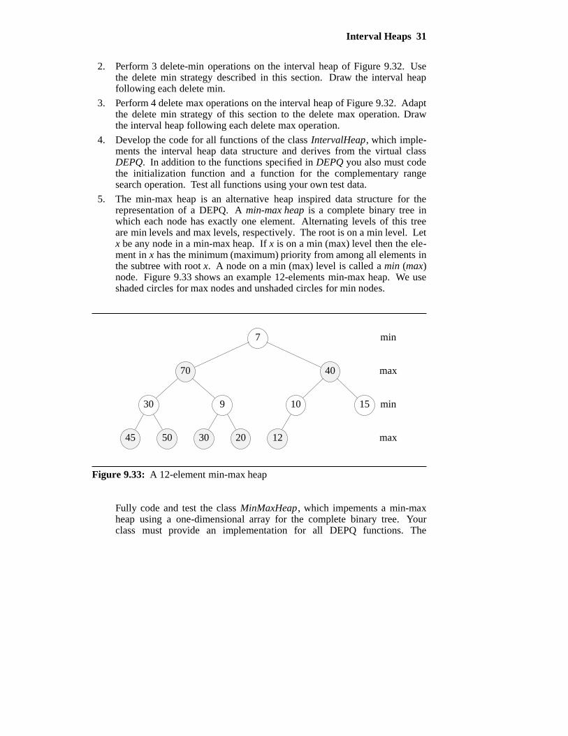
5. The min-max heap is an alternative heap inspired data structure for therepresentation of a DEPQ. A min-max heap is a complete binary tree inwhich each node has exactly one element. Alternating levels of this treeare min levels and max levels, respectively. The root is on a min level. Letx be any node in a min-max heap. If x is on a min (max) level then the ele-ment in x has the minimum (maximum) priority from among all elements inthe subtree with root x. A node on a min (max) level is called a min (max)node. Figure 9.33 shows an example 12-elements min-max heap. We useshaded circles for max nodes and unshaded circles for min nodes.

45 50 30 20 12

30 9 10 15

70 40

7

max

min

max

min

Figure 9.33: A 12-element min-max heap

Fully code and test the class MinMaxHeap, which impements a min-maxheap using a one-dimensional array for the complete binary tree. Yourclass must provide an implementation for all DEPQ functions. The

32 Priority Queues

complexity of GetMin and GetMax should be Ο(1) and that for the remain-ing DEPQ functions should be Ο(log n).

9.4 REFERENCES AND SELECTED READINGS

Height-biased leftist trees were invented by C. Crane. See, Linear Lists andPriority Queues as Balanced Binary Trees, Technical report CS-72-259, Com-puter Science Dept., Stanford University, Palo Alto, CA, 1972. Weight-biasedleftist trees were developed in ‘‘Weight biased leftist trees and modified skiplists,’’ S. Cho and S. Sahni, ACM Jr. on Experimental Algorithms, Article 2,1998.

The exercise on lazy deletion is from ‘‘Finding minimum spanning trees,’’by D. Cheriton and R. Tarjan, SIAM Journal on Computing, 5, 1976, pp. 724-742.

B-heaps and F-heaps were invented by M. Fredman and R. Tarjan. Theirwork is reported in the paper ‘‘Fibonacci heaps and their uses in improved net-work optimization algorithms,’’ JACM, 34:3, 1987, pp. 596-615. This paper alsodescribes several variants of the basic F-heap as discussed here, as well as theapplication of F-heaps to the assignment problem and to the problem of finding aminimum-cost spanning tree. Their result is that using F-heaps, minimum-costspanning trees can be found in Ο(eβ(e,n)) time, where β(e,n) ≤ log*n whene ≥ n. log*n = mini | log(i)n ≤ 1, log(0)n = n, and log(i)n = log(log(i −1)n). Thecomplexity of finding minimum-cost spanning trees has been further reduced toΟ(elogβ(e,n)). The reference for this is ‘‘Efficient algorithms for findingminimum spanning trees in undirected and directed graphs,’’ by H. Gabow, Z.Galil, T. Spencer, and R. Tarjan, Combinatorica, 6:2, 1986, pp. 109-122.

Pairing heaps were developed in the paper ‘‘The pairing heap: A new formof self-adjusting heap’’, by M. Fredman, R. Sedgewick, R. Sleator, and R. Tarjan,Algorithmica, 1, 1986, pp. 111-129. This paper together with ‘‘New upperbounds for pairing heaps,’’ by J. Iacono, Scandinavian Workshop on AlgorithmTheory, LNCS 1851, 2000, pp. 35-42 establishes the amortized complexity of thepairing heap operations. The paper ‘‘On the efficiency of pairing heaps andrelated data structures,’’ by M. Fredman, Jr. of the ACM, 46, 1999, pp. 473-501provides an information theoretic proof that Ω(log log n) is a lower bound on theamortized complexity of the decrease key operation for pairing heaps.

Experimental studies conducted by Stasko and Vitter reported in theirpaper ‘‘Pairing heaps: Experiments and analysis,’’ Communications of the ACM,30, 3, 1987, 234-249 establish the superiority of two pass pairing heaps overmultipass pairing heaps. This paper also proposes a variant of pairing heaps(called auxiliary two pass pairing heaps) that performs better than two pass pair-ing heaps. Moret and Shapiro establish the superiority of pairing heaps over

References and Selected Readings 33

Fibonacci heaps, when implementing Prim’s minimum spanning tree algorithm,in their paper ‘‘An empirical analysis of algorithms for for constructing aminimum cost spanning tree,’’ Second Workshop on Algorithms and Data Struc-tures, 1991, pp. 400-411.

A large number of data structures, inspired by the fundamental heap struc-ture of Section 5.6, have been developed for the representation of a DEPQ. Thesymmetric min-max heap was developed in ‘‘Symmetric min-max heap: Asimpler data structure for double-ended priority queue,’’ by A. Arvind and C.Pandu Rangan, Information Processing Letters, 69, 1999, 197-199.

The twin heaps of Williams, the min-max pair heapsof Olariu et al., theinterval heaps of Ding and Weiss and van Leeuwen et al., and the diamonddeques of Chang and Du are virtually identical data structures. The relevantpapers are: ‘‘Diamond deque: A simple data structure for priority deques,’’ by S.Chang and M. Du, Information Processing Letters, 46, 231-237, 1993; ‘‘On theComplexity of Building an Interval Heap,’’ by Y. Ding and M. Weiss, Informa-tion Processing Letters, 50, 143-144, 1994; ‘‘Interval heaps,’’ by J. van Leeuwenand D. Wood, The Computer Journal, 36, 3, 209-216, 1993; ‘‘A mergeabledouble-ended priority queue,’’ by S. Olariu, C. Overstreet, and Z. Wen, TheComputer Journal, 34, 5, 423-427, 1991; and ‘‘Algorithm 232,’’ by J. Williams,Communications of the ACM, 7, 347-348, 1964.

The min-max heap and deap are additional heap-inspired stuctures forDEPQs. These data structures were developed in ‘‘Min-max heaps and general-ized priority queues,’’ by M. Atkinson, J. Sack, N. Santoro, and T. Strothotte,Communications of the ACM, 29:10, 1986, pp. 996-1000 and ‘‘The deap: Adouble-ended heap to implement double-ended priority queues,’’ by S. Carlsson,Information Processing Letters, 26, 1987, pp. 33-36, respectively.

Data structures for meldable DEPQs are developed in ‘‘The relaxed min-max heap: A mergeable double-ended priority queue,’’ by Y. Ding and M. Weiss,Acta Informatica, 30, 215-231, 1993; ‘‘Fast meldable priority queues,’’ by G.Brodal, Workshop on Algorithms and Data Structures, 1995 and ‘‘Mergeabledouble ended priority queue,’’ by S. Cho and S. Sahni, International Journal onFoundation of Computer Sciences , 10, 1, 1999, 1-18.

General techniques to arrive at a data structure for a DEPQ from one for asingle-ended priority queue are developed in ‘‘Correspondence based data struc-tures for double ended priority queues,’’ by K. Chong and S. Sahni, ACM Jr. onExperimental Algorithmics, Volume 5, 2000, Article 2.

For more on priority queues, see Chapters 5 through 8 of ‘‘Handbook ofdata structures and applications,’’ edited by D. Mehta and S. Sahni, Chapman &Hall/CRC, Boca Raton, 2005.

-- --

priority queues - uqacalthough the amortized complexity is better when a fibonacci heap is used...

Documents