privacy preserving categorical data analysis with unknown ... · transactions on data privacy 2...

TRANSACTIONS ONDATA PRIVACY 2 (2009) 185–205

Privacy Preserving Categorical DataAnalysis with Unknown DistortionParametersLing Guo∗, Xintao Wu∗

∗Software and Information Systems Department, University of North Carolina at Charlotte, Charlotte, NC 28223, USA.

E-mail: {lguo2,xwu}@uncc.edu

Abstract. Randomized Response techniques have been investigated in privacy preserving categorical dataanalysis. However, the released distortion parameters canbe exploited by attackers to breach privacy. In thispaper, we investigate whether data mining or statistical analysis tasks can still be conducted on randomized datawhen distortion parameters are not disclosed to data miners. We first examine how various objective associationmeasures between two variables may be affected by randomization. We then extend to multiple variables byexamining the feasibility of hierarchical loglinear modeling. Finally we show some classic data mining tasksthat cannot be applied on the randomized data directly.

1 Introduction

Privacy is becoming an increasingly important issue in manydata mining applications. A con-siderable amount of work on randomization based privacy preserving data mining (for numericaldata [1, 3, 23, 24], categorical data [4, 22], market basket data [19, 31], and linked data [21, 27, 37])has been investigated recently.Randomization still runs certain risk of disclosures. Attackers may exploit the released distortion

parameters to calculate the posterior probabilities of theoriginal value based on the distorted data.It is considered to be jeopardizing with respect to the original value if the posterior probabilities aresignificantly greater than the a-priori probabilities. In this paper, we consider the scenario where thedistortion parameters are not released in order to prevent attackers from exploiting those distortionparameters to recover individual data.In the first part of our paper, we investigate how various objective measures used for association

analysis between two variables may be affected by randomization. We demonstrate that some mea-sures (e.g., Correlation, Mutual Information, LikelihoodRatio, Pearson Statistics) have a verticalmonotonic property , i.e., the values calculated directly from the randomized data are always lessthan or equal to those original ones. Hence, some data analysis tasks (e.g., independence testing)can be executed on the randomized data directly even withoutknowing distortion parameters. Wethen investigate how the relative order of two association patterns is affected when the same random-ization is conducted. We show that some measures (e.g., Piatetsky-Shapiro) have relative horizontalorder invariant properties, i.e, if one pattern is strongerthan another in the original data, we havethat the first one is still stronger than the second one in the randomized data.In the second part of our paper, we extend association analysis from two variables to multiple

variables. We investigate the feasibility of loglinear modeling, which is well adopted to analyze

185

186 Ling Guo, Xintao Wu

associations among three or more variables, and examine thecriterion on determining which hierar-chical loglinear models are preserved in the randomized data. We also show that several multi-variateassociation measures studied in the data mining community are special cases of loglinear modeling.Finally, we demonstrate the infeasibility of some classic data mining tasks (e.g., association rule

mining, decision tree learning, naıve Bayesian classifier) on randomized data by showing the non-monotonic properties of measures (e.g.,support/confidence, gini) adopted in those data mining tasks.Our motivation is to provide a reference to data miners aboutwhat they can do and what they cannot do with certainty upon the randomized data directly without distortion parameters. To the bestof our knowledge, this is the first such formal analysis of theeffects of Randomized Response forprivacy preserving categorical data analysis with unknowndistortion parameters.

2 Related Work

Privacy is becoming an increasingly important issue in manydata mining applications. A consider-able amount of work on privacy preserving data mining, such as additive randomization based [1,3]has been proposed. Recently, a lot of research has focused onthe privacy aspect of the above ap-proaches and various point-wise reconstruction methods [23,24] have been investigated.The issue of maintaining privacy in association rule miningand categorical data analysis has also

attracted considerable studies [4,11,14,15,31]. Most of techniques are based on a data perturbationor Randomized Response (RR) approach [7]. In [31], the authors proposed the MASK technique topreserve privacy for frequent itemset mining and extended to general categorical attributes in [4]. In[11], the authors studied the use of randomized response technique to build decision tree classifiers.In [19,20], the authors focused on the issue of providing accuracy in terms of various reconstructedmeasures (e.g., support, confidence, correlation, lift, etc.) in privacy preserving market basket dataanalysis when the distortion parameters are available. Recently, the authors in [22] studied the searchof optimal distortion parameters to balance privacy and utility.Most of previous work except [19] investigated the scenariothat distortion parameters are fully

or partially known by data miners. For example, the authors in [13] focused on measuring privacyfrom attackers view when the distorted records of individuals and distortion parameters (e.g.,fY

andP ) are available. In [19], the authors very briefly showed thatsome measures have verticalmonotonic property on the market basket data. In this paper,we present a complete framework onprivacy preserving categorical data analysis without distortion parameters. We extend studies onassociation measures between two binary variables to thoseon multiple polychotomous variables.More importantly, we also propose a new type of monotonic property,horizontal association, i.e.,according to some measures, if the association between one pair of variables is stronger than anotherin the original data, the same order will still be kept in the randomized data when the same level ofrandomization is applied.Randomized Response (RR) techniques have also been extensively investigated in statistics (e.g.,

see a book [7]). The Post RAndomization Method (PRAM) has been proposed to prevent disclosurein publishing micro data [9,17,18,35,36]. Specifically, they studied how to choose transition prob-abilities (a.k.a. distortion parameters) such that certain chosen marginal distributions in the originaldata are left invariant in expectation of the randomized data. There are some other noise-additionmethods have been investigated in the literature, see the excellent survey [6]. Authors in [25] pro-posed a method by additional transformations that guarantees the covariance matrix of the distortedvariables is an unbiased estimate for the one of the originalvariables. The method works well fornumerical variables, but it is difficult to be applied to categorical variables due to the structure of thetransformations.Recently, the role of background knowledge in privacy preserving data mining has been studied

TRANSACTIONS ONDATA PRIVACY 2 (2009)

Privacy Preserving Categorical Data Analysis with UnknownDistortion Parameters 187

Table 1: COIL significant attributes used in example. The column “Mapping” shows how to mapeach original variable to a binary variable.

attribute i−th attribute Name Description MappingA 18 MOPLLAAG Lower level education > 4 → 1B 37 MINKM30 Income< 30K > 4 → 1C 42 MINKGEM Average income > 4 → 1D 43 MKOOPKLA Purchasing power class> 3 → 1E 44 PWAPART Contribution private third party insurance> 0 → 1F 47 PPERSAUT Contribution car policies > 0 → 1G 59 PBRAND Contribution fire policies > 0 → 1H 65 AWAPART Number of private third party insurance> 0 → 1I 68 APERSAUT Number of car policies > 0 → 1J 86 CARAVAN Number of mobile home policies > 0 → 1

[10,28]. Their focus was on disclosure risk due to the effectof various background knowledge. Thefocus of our work is on data utility when the distortion parameters are not available. We considerthe extreme scenario about what data miners can do and can notdo with certainty upon randomizeddata directly without any other background knowledge. Privacy analysis is beyond the scope of thispaper and will be addressed in our future work.

3 Preliminaries

Throughout this paper, we use the COIL Challenge 2000 which provides data from a real insurancebusiness. Information about customers consists of 86 attributes and includes product usage data andsocio-demographic data derived from zip area codes. Our binary data is formed by collapsing non-binary categorical attributes into binary form, with5822 records and86 binary attributes. We useten attributes (denote asA to J) as shown in Table 1 to illustrate our results.

3.1 Notations

To be consistent with notations, we denote the set of recordsin the databaseD by T = {T0,· · · , TN−1} and the set of variables byI = {A0, · · · , Am−1, B0, · · · , Bn−1}. Note that, for ease ofpresentation, we use the terms “attribute” and “variable” interchangeably. Let there bem sensitivevariablesA0, · · · , Am−1 andn non-sensitive variablesB0, · · · , Bn−1. Each variableAu hasdu

mutually exclusive and exhaustive categories. We useiu = 0, · · · , du − 1 to denote the index ofits categories. For each record, we apply the Randomized Response model independently on eachsensitive variableAu using different settings of distortion, while keeping the non-sensitive onesunchanged.To express the relationship among variables, we can map categorical data sets to contingency tables.

Table 2(a) shows one contingency table for a pair of two variables,GenderandRace(d1 = 2 andd2 = 3). The vectorπ = (π00, π01, π02,π10, π11, π12)

′

corresponds to a fixed order of cell entriesπij in the2 × 3 contingency table.π01 denotes the proportion of records withMaleandWhite. Therow sumπ0+ represents the proportion of records withMale across all races.



Table 2:2 × 3 contingency tables for two variables Gender, Race(a) Original

Black White AsianMale π00 π01 π02 π0+

Female π10 π11 π12 π1+

π+0 π+1 π+2 π++

(b) After randomization

Black White AsianMale λ00 λ01 λ02 λ0+

Female λ10 λ11 λ12 λ1+

λ+0 λ+1 π+2 λ++

Table 3: NotationSymbol Definition

Au theuth variable which is sensitiveBl thelth variable which is not sensitivePu distortion matrix ofAu

θ(u) distortion parameter ofAu

Au variableAu after randomizationχ2

ori χ2 calculated from original dataχ2

ran χ2 calculated from randomized dataπi0,··· ,ik−1 cell value of original contingency tableλi0,··· ,ik−1 cell value of randomized contingency table

Formally, letπi0,··· ,ik−1denotes the true proportion corresponding to the categorical combination of

k variables(A0i0 , · · · , A(k−1)ik−1) in the original data, whereiu = 0, · · · , du−1; u = 0, · · · , k−1,

andA0i0 denotes thei0th category of attributeA0. Let π be a vector with elementsπi0,··· ,ik−1

arranged in a fixed order. The combination vector corresponds to a fixed order of cell entries inthe contingency table formed by thesek variables. Similarly, we denoteλi0,··· ,ik−1

as the expectedproportion in the randomized data. Table 3 summarizes our notations.

3.2 Distortion Procedure

The first Randomized Response model proposed by Warner in 1965 dealt with one dichotomous at-tribute, i.e, every person in the population belongs to either a sensitive groupA, or to its complementA. The problem is to estimate theπA, the unknown proportion of population members in groupA.Each respondent is provided with a randomization device by which the respondent chooses one ofthe following two questionsDo you belong to A?or Do you belong toA? with respective probabili-tiesp and1 − p and then repliesyesor no to the question chosen. Since no one but the respondentknows to which question the answer pertains, the technique provides response confidentiality andincreases respondents’ willingness to answer sensitive questions. In general, we can consider thisdichotomous attribute as one{0, 1} variable, e.g., with 0 = absence, 1= presence. Each record isindependently randomized using the probability matrix

P =

(

θ0 1 − θ1

1 − θ0 θ1

)

(1)

If the original record is in theabsence(presence) category, it will be kept in such category with aprobabilityθ0 (θ1) and changed topresence(absence) category with a probability1 − θ0 (1 − θ1).The original Warner RR model simply setsθ0 = θ1 = p.We extend RR to the scenario of multi-variables with multi-categories in our distortion framework.

For one sensitive variableAu with du categories, the randomization process is such that a record



belong to thejth category (j = 0, ..., du − 1) is distorted to 0, 1, ... ordu − 1th category withrespective probabilitiesθ(u)

j0 , θ(u)j1 , ..., θ

(u)j du−1, where

∑du−1c=0 θ

(u)jc = 1. The distortion matrixPu for

Au is shown as below.

Pu =

θ(u)00 θ

(u)10 · · · θ

(u)du−1 0

θ(u)01 θ

(u)11 · · · θ

(u)du−1 1

.

.

θ(u)0 du−1 θ

(u)1 du−1 · · · θ

(u)du−1 du−1

Parameters in each column ofPu sum to1, but are independent to parameters in other columns. Thesum of parameters in each row is not necessarily equal to1. The true proportionπ = (π0, · · · , πdu−1)is changed toλ = (λ0, · · · , λdu−1) after randomization. We have

λ = Puπ.

For the case ofk multi-variables, we denoteλµ0,··· ,µk−1as the expected probability of getting a

response(A0µ0 , · · · , A(k−1)µk−1) andλ the vector with elementsλµ0,··· ,µk−1

arranged in a fixedorder (e.g., the vectorλ = (λ00, λ01, λ02, λ10, λ11, λ12)

′ corresponds to cell entriesλij in therandomized contingency table as shown in Table 2(b) ). LetP = P0 × · · · × Pk−1, we can obtain

λ = Pπ = (P0 × · · · × Pk−1)π (2)

where× stands for the Kronecker product1.The original databaseD is changed toDran after randomization. An unbiased estimate ofπ based

on one given realizationDran follows as

π = P−1λ = (P−10 × · · · × P−1

k−1)λ (3)

whereλ is the vector of proportions calculated fromDran corresponding toλ andP−1u denotes the

inverse of the matrixPu.Previous work using RR model either focused on evaluating the trade-off between privacy preserva-

tion and utility loss of the reconstructed data with the released distortion parameters (e.g., [4,19,31])or determining the optimal distortion parameters to achieve good performance (e.g., [22]). Datamining tasks were conducted on the reconstructed distribution π calculated from Equation 3. Inthis paper, we investigate the problem whether data mining or statistical analysis tasks can still beconducted with unknown distortion parameters, which has not been studied in the literature.In Lemma 1, we show that no monotonic relation exists for cellentries of contingency tables due

to randomization.

Lemma 1. No monotonic relation exists betweenλi0,··· ,ik−1andπi0,··· ,ik−1

.

Proof. We use two binary variablesAu, Av as an example. The proof of multiple variables withmulti-categories is immediate. The distortion matrices are defined as:

Pu =

(

θ(u)0 1 − θ

(u)1

1 − θ(u)0 θ

(u)1

)

Pv =

(

θ(v)0 1 − θ

(v)1

1 − θ(v)0 θ

(v)1

)

1It is an operation on two matrices, anm-by-n matrix A and ap-by-q matrix B, resulting in themp-by-nq block matrix



We have:

λ0+ = (θ(u)0 + θ

(u)1 − 1)π0+ − θ

(u)1 + 1

We can see thatλ0+ − π0+ is a function ofπ0+ ,θ(u)0 , θ

(u)1 , and its value may be greater or less than

0 with varying distortion parameters. Similarly,

λ00 = θ(u)0 θ

(v)0 π00 + θ

(u)0 (1 − θ

(v)1 )π01

+ (1 − θ(u)1 )θ

(v)0 π10 + (1 − θ

(u)1 )(1 − θ

(v)1 )π11

λ00 − π00 is a function ofπij ,θ(u)0 , θ

(u)1 , θ

(v)0 andθ

(v)1 , no monotonic relation exists.

4 Associations Between Two Variables

In this section, we investigate how associations between two variables are affected by randomization.Specifically, we consider two cases:

• Case 1: Au andAv, association between two sensitive variables.

• Case 2: Au andBl, association between a sensitive variable and a non-sensitive variable.

Case 2 is a special case of case 1 whilePl is an identity matrix, so any results for case 1 will satisfycase 2. However, it is not necessarily true vice versa.

4.1 Associations Between Two Binary Variables

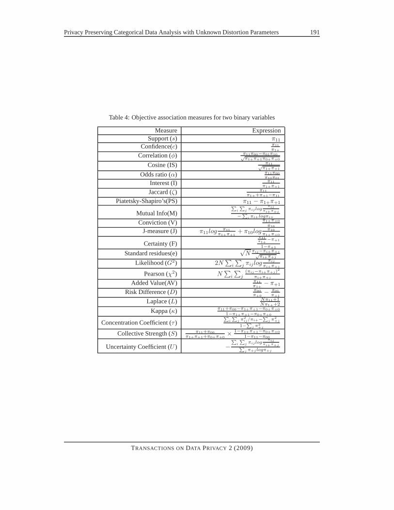
Table 4 shows various association measures for two binary variables (Refer to [34] for a survey). Wecan observe that all measures can be expressed as functions with parameters as cell entries (πij) andtheir margin totals (πi+ or π+j) in the 2-dimensional contingency table.Randomization SettingFor a binary variableAu, which only has two categories (0 = absence, 1 =presence), the distortion parameters are the same as those in Equation 1.In Section 4.1.1, we focus on the problem of vertical association variation, i.e., how association

values of one pair of variables based on given measures are changed due to randomization. InSection 4.1.2, we focus on the problem of horizontal association variation, i.e., how the relativeorder of two association patterns is changed due to randomization.

4.1.1 Vertical Association Variation

We use subscriptsori andran to denote measures calculated from the original data and random-ized data (without knowing the distortion parameters) respectively. For example,χ2

ori denotes thePearson Statistics calculated from the original dataD while χ2

ran corresponds to the one calculateddirectly from the randomized dataDran.There exist many different realizationsDran for one original data setD. When the data size is

large, the distributionλ calculated from one realizationDran approaches its expectationλ, whichcan be calculated from the distributionπ of the original data set through Equation 2. This is because

cov(λ) = N−1(λδ − λλ′),

as shown in [7].cov(λ) approaches zero whenN is large. Hereλδ is a diagonal matrix with thesame diagonal elements as those ofλ arranged in the same order. All our following results and their



Table 4: Objective association measures for two binary variables

Measure ExpressionSupport (s) π11

Confidence(c) π11

π1+

Correlation (φ) π11π00−π01π10√π1+π+1π0+π+0

Cosine (IS) π11√π1+π+1

Odds ratio (α) π11π00

π10π01

Interest (I) π11

π1+π+1

Jaccard (ζ) π11

π1++π+1−π11

Piatetsky-Shapiro’s(PS) π11 − π1+π+1

Mutual Info(M)P

i

P

j πij logπij

πi+π+j

−P

i πi+logπi+

Conviction (V) π1+π+0

π10

J-measure (J) π11logπ11

π1+π+1+ π10log

π10

π1+π+0

Certainty (F)π11π1+

−π+1

1−π+1

Standard residues(e)√

Nπij−πi+π+j√

πi+π+j

Likelihood (G2) 2N∑

i

∑

j πij logπij

πi+π+j

Pearson (χ2) N∑

i

∑

j(πij−πi+π+j)

2

πi+π+j

Added Value(AV) π11

π1+− π+1

Risk Difference (D) π00

π+0− π01

π+1

Laplace (L) Nπ11+1Nπ1++2

Kappa (κ) π11+π00−π1+π+1−π0+π+0

1−π1+π+1−π0+π+0

Concentration Coefficient (τ )P

i

P

jπ2

ij/πi+−P

jπ2+j

1−P

j π2+j

Collective Strength (S) π11+π00

π1+π+1+π0+π+0× 1−π1+π+1−π0+π+0

1−π11−π00

Uncertainty Coefficient (U ) −P

i

P

j πij logπij

πi+π+jP

j π+j logπ+j



proofs are based on the expectationλ, rather than a given realizationλ. Since data sets are usuallylarge in most data mining scenarios, we do not consider the effect due to small samples. In otherwords, our results are expected to hold for most realizations of the randomized data.

Result 1. For any pair of variablesAu, Av perturbed with any distortion matrixPu andPv (θ(u)0 ,

θ(u)1 , θ

(v)0 , θ

(v)1 ∈ [0, 1]) respectively (Case 1), or any pair of variablesAu, Bl whereAu is perturbed

with Pu (Case 2), theχ2, G2, M, τ, U, φ, D, PS values calculated from both original and random-ized data satisfy:

χ2ran ≤ χ2

ori, G2ran ≤ G2

ori

Mran ≤ Mori, τran ≤ τori

Uran ≤ Uori, |φran| ≤ |φori||Dran| ≤ |Dori|, |PSran| ≤ |PSori|

No other measures shown in Table 4 holds monotonic property.

For randomization, we know that the distortion is 1) highestwith θ = 0.5 which imparts the max-imum randomness to the distorted values; 2) symmetric around θ = 0.5 and makes no difference,reconstruction-wise, between choosing a valueθ or its counterpart1 − θ. In practice, the distortionis usually conducted withθ greater than 0.5. The following results show the vertical associationvariations whenθ(u)

0 ,θ(u)1 ,θ(v)

0 andθ(v)1 are greater than 0.5.

Result 2. In addition to monotonic relations shown in Result 1, whenθ(u)0 , θ(u)

1 , θ(v)0 , θ(v)

1 ∈ [0.5, 1],we have

|Fran| ≤ |Fori|, |AVran| ≤ |AVori||κran| ≤ |κori|, |αran − 1| ≤ |αori − 1|

|Iran − 1| ≤ |Iori − 1|, |Vran − 1| ≤ |Vori − 1||Sran − 1| ≤ |Sori − 1|

We include the proof of Added ValueAV in Appendix. For all other measures in the above tworesults, we can prove similarly. We skip their proofs due to space limits. We can see that fourmeasures ( Odds Ratioα, Collective StrengthS, InterestPS, and ConvictionV ) are compared with“1” since values of these measures with “1” indicate the two variables are independent. Next weillustrate this monotonic property using an example.

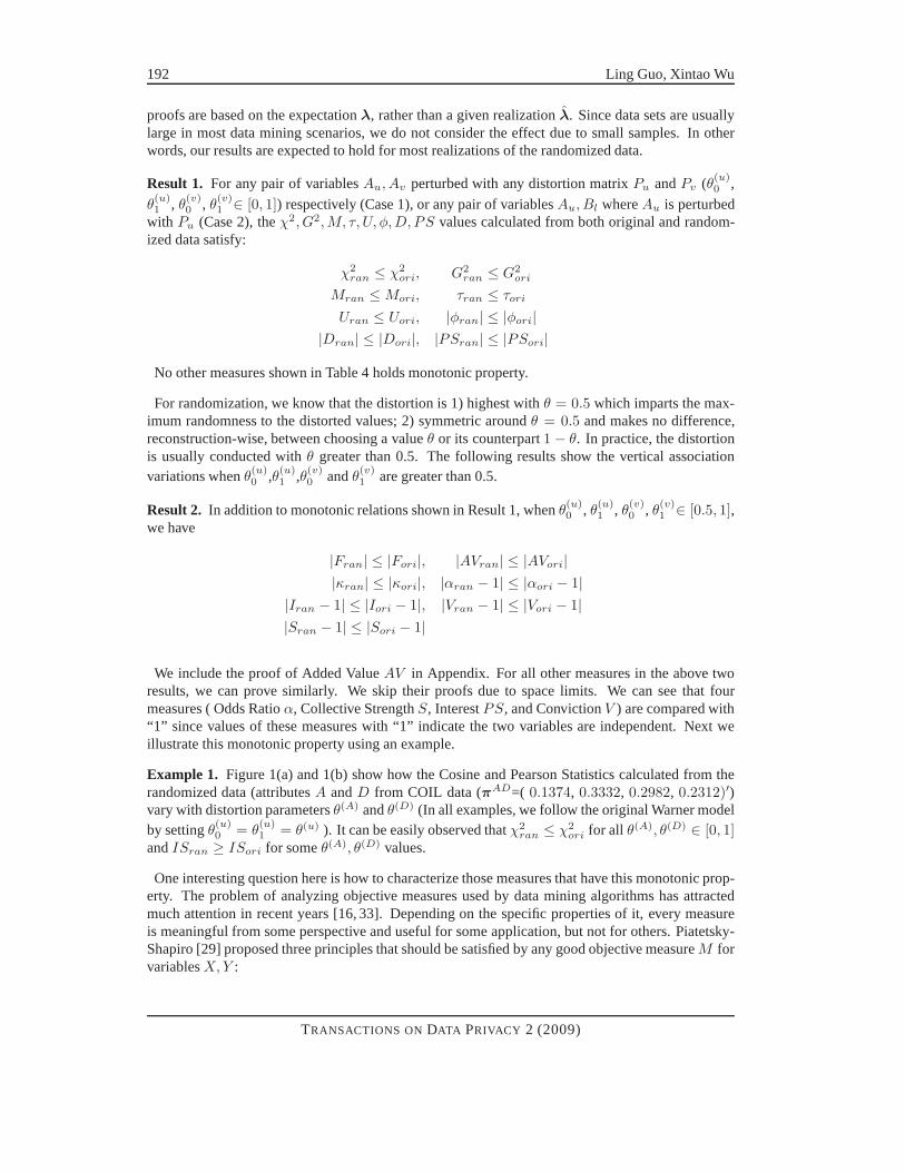
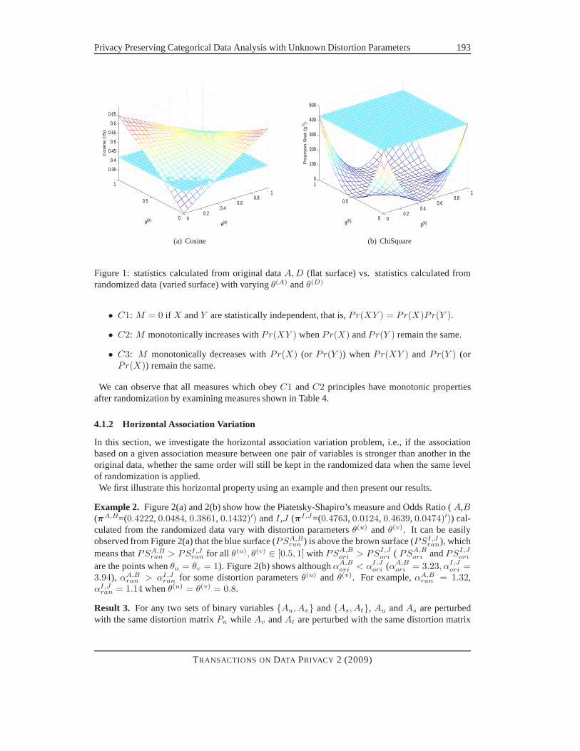
Example 1. Figure 1(a) and 1(b) show how the Cosine and Pearson Statistics calculated from therandomized data (attributesA andD from COIL data (πAD=( 0.1374, 0.3332, 0.2982, 0.2312)′)vary with distortion parametersθ(A) andθ(D) (In all examples, we follow the original Warner modelby settingθ(u)

0 = θ(u)1 = θ(u) ). It can be easily observed thatχ2

ran ≤ χ2ori for all θ(A), θ(D) ∈ [0, 1]

andISran ≥ ISori for someθ(A), θ(D) values.

One interesting question here is how to characterize those measures that have this monotonic prop-erty. The problem of analyzing objective measures used by data mining algorithms has attractedmuch attention in recent years [16, 33]. Depending on the specific properties of it, every measureis meaningful from some perspective and useful for some application, but not for others. Piatetsky-Shapiro [29] proposed three principles that should be satisfied by any good objective measureM forvariablesX, Y :



00.2

0.40.6

0.81

0

0.5

1

0.35

0.4

0.45

0.5

0.55

0.6

0.65

θ(A)θ(D)

Co

sin

e (

IS)

(a) Cosine

00.2

0.40.6

0.81

0

0.5

10

100

200

300

400

500

θ(A)θ(D)

Pe

ars

on

Sta

t (χ

2)

(b) ChiSquare

Figure 1: statistics calculated from original dataA, D (flat surface) vs. statistics calculated fromrandomized data (varied surface) with varyingθ(A) andθ(D)

• C1: M = 0 if X andY are statistically independent, that is,Pr(XY ) = Pr(X)Pr(Y ).

• C2: M monotonically increases withPr(XY ) whenPr(X) andPr(Y ) remain the same.

• C3: M monotonically decreases withPr(X) (or Pr(Y )) whenPr(XY ) andPr(Y ) (orPr(X)) remain the same.

We can observe that all measures which obeyC1 andC2 principles have monotonic propertiesafter randomization by examining measures shown in Table 4.

4.1.2 Horizontal Association Variation

In this section, we investigate the horizontal associationvariation problem, i.e., if the associationbased on a given association measure between one pair of variables is stronger than another in theoriginal data, whether the same order will still be kept in the randomized data when the same levelof randomization is applied.We first illustrate this horizontal property using an example and then present our results.

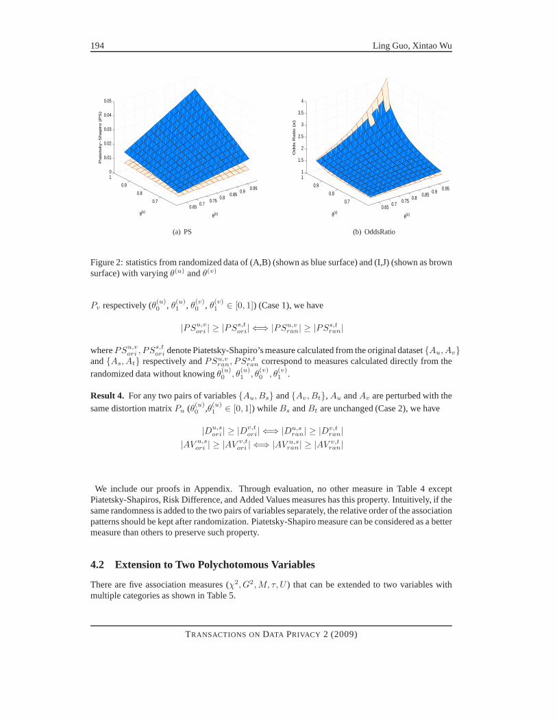
Example 2. Figure 2(a) and 2(b) show how the Piatetsky-Shapiro’s measure and Odds Ratio (A,B(πA,B=(0.4222, 0.0484, 0.3861, 0.1432)′) andI,J (πI,J=(0.4763, 0.0124, 0.4639, 0.0474)′)) cal-culated from the randomized data vary with distortion parametersθ(u) andθ(v). It can be easilyobserved from Figure 2(a) that the blue surface (PSA,B

ran ) is above the brown surface (PSI,Jran), which

means thatPSA,Bran > PSI,J

ran for all θ(u), θ(v) ∈ [0.5, 1] with PSA,Bori > PSI,J

ori ( PSA,Bori andPSI,J

ori

are the points whenθu = θv = 1). Figure 2(b) shows althoughαA,Bori < αI,J

ori (αA,Bori = 3.23, αI,J

ori =3.94), αA,B

ran > αI,Jran for some distortion parametersθ(u) andθ(v). For example,αA,B

ran = 1.32,αI,J

ran = 1.14 whenθ(u) = θ(v) = 0.8.

Result 3. For any two sets of binary variables{Au, Av} and{As, At}, Au andAs are perturbedwith the same distortion matrixPu while Av andAt are perturbed with the same distortion matrix



0.650.7

0.750.8

0.850.9

0.95

0.7

0.8

0.9

10

0.01

0.02

0.03

0.04

0.05

θ(u)θ(v)

Pia

tets

ky−

Sh

ap

iro

(P

S)

(a) PS

0.650.7

0.750.8

0.850.9

0.95

0.7

0.8

0.9

11

1.5

2

2.5

3

3.5

4

θ(u)θ(v)

Od

ds R

atio

(α

)

(b) OddsRatio

Figure 2: statistics from randomized data of (A,B) (shown asblue surface) and (I,J) (shown as brownsurface) with varyingθ(u) andθ(v)

Pv respectively (θ(u)0 , θ

(u)1 , θ

(v)0 , θ

(v)1 ∈ [0, 1]) (Case 1), we have

|PSu,vori | ≥ |PSs,t

ori| ⇐⇒ |PSu,vran| ≥ |PSs,t

ran|

wherePSu,vori , PSs,t

ori denote Piatetsky-Shapiro’s measure calculated from the original dataset{Au, Av}and{As, At} respectively andPSu,v

ran, PSs,tran correspond to measures calculated directly from the

randomized data without knowingθ(u)0 , θ

(u)1 , θ

(v)0 , θ

(v)1 .

Result 4. For any two pairs of variables{Au, Bs} and{Av, Bt}, Au andAv are perturbed with the

same distortion matrixPu (θ(u)0 ,θ(u)

1 ∈ [0, 1]) while Bs andBt are unchanged (Case 2), we have

|Du,sori| ≥ |Dv,t

ori| ⇐⇒ |Du,sran| ≥ |Dv,t

ran||AV u,s

ori | ≥ |AV v,tori | ⇐⇒ |AV u,s

ran| ≥ |AV v,tran|

We include our proofs in Appendix. Through evaluation, no other measure in Table 4 exceptPiatetsky-Shapiros, Risk Difference, and Added Values measures has this property. Intuitively, if thesame randomness is added to the two pairs of variables separately, the relative order of the associationpatterns should be kept after randomization. Piatetsky-Shapiro measure can be considered as a bettermeasure than others to preserve such property.

4.2 Extension to Two Polychotomous Variables

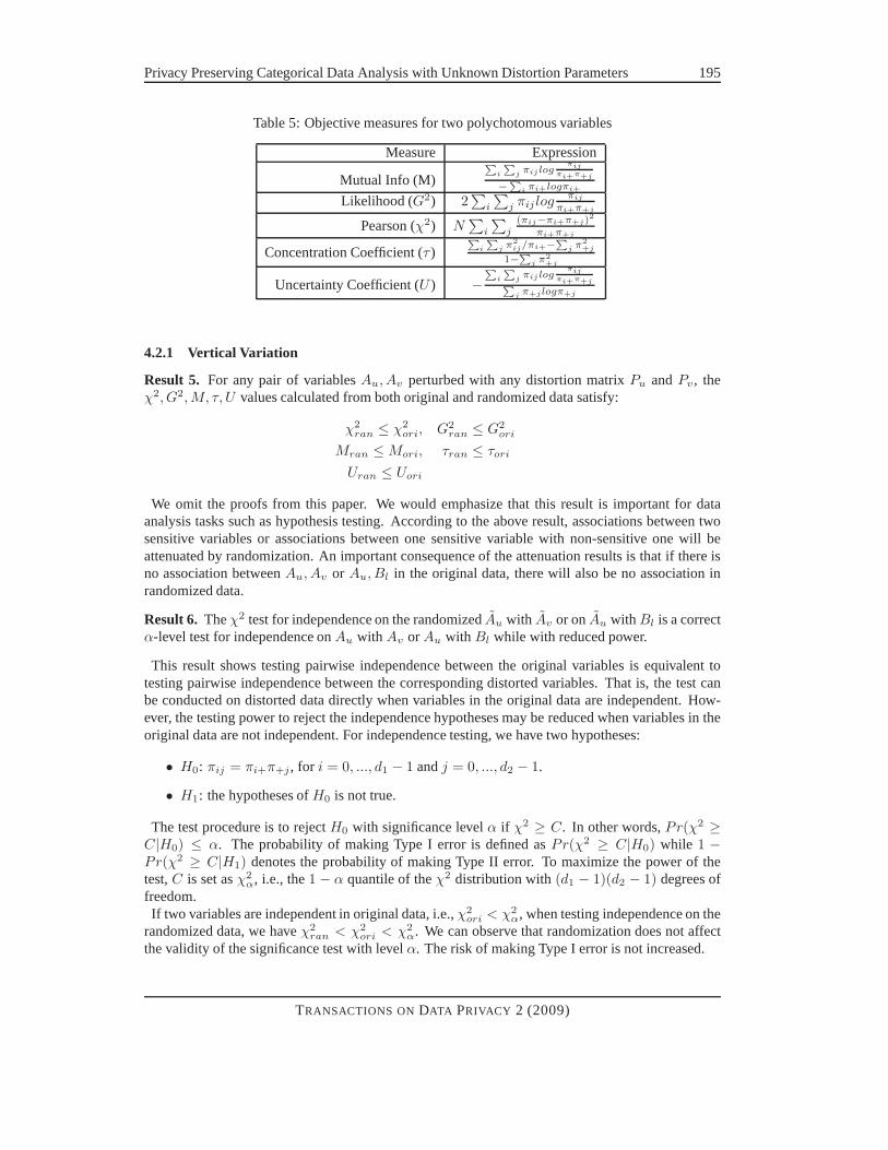
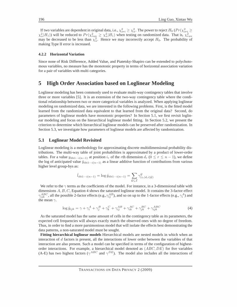
There are five association measures (χ2, G2, M, τ, U ) that can be extended to two variables withmultiple categories as shown in Table 5.



Table 5: Objective measures for two polychotomous variables

Measure Expression

Mutual Info (M)P

i

P

jπij log

πij

πi+π+j

− P

iπi+logπi+

Likelihood (G2) 2∑

i

∑

j πij logπij

πi+π+j

Pearson (χ2) N∑

i

∑

j(πij−πi+π+j)

2

πi+π+j

Concentration Coefficient (τ )P

i

P

jπ2

ij/πi+−P

jπ2+j

1−P

j π2+j

Uncertainty Coefficient (U ) −P

i

P

jπij log

πij

πi+π+jP

jπ+jlogπ+j

4.2.1 Vertical Variation

Result 5. For any pair of variablesAu, Av perturbed with any distortion matrixPu andPv, theχ2, G2, M, τ, U values calculated from both original and randomized data satisfy:

χ2ran ≤ χ2

ori, G2ran ≤ G2

ori

Mran ≤ Mori, τran ≤ τori

Uran ≤ Uori

We omit the proofs from this paper. We would emphasize that this result is important for dataanalysis tasks such as hypothesis testing. According to theabove result, associations between twosensitive variables or associations between one sensitivevariable with non-sensitive one will beattenuated by randomization. An important consequence of the attenuation results is that if there isno association betweenAu, Av or Au, Bl in the original data, there will also be no association inrandomized data.

Result 6. Theχ2 test for independence on the randomizedAu with Av or onAu with Bl is a correctα-level test for independence onAu with Av or Au with Bl while with reduced power.

This result shows testing pairwise independence between the original variables is equivalent totesting pairwise independence between the corresponding distorted variables. That is, the test canbe conducted on distorted data directly when variables in the original data are independent. How-ever, the testing power to reject the independence hypotheses may be reduced when variables in theoriginal data are not independent. For independence testing, we have two hypotheses:

• H0: πij = πi+π+j , for i = 0, ..., d1 − 1 andj = 0, ..., d2 − 1.

• H1: the hypotheses ofH0 is not true.

The test procedure is to rejectH0 with significance levelα if χ2 ≥ C. In other words,Pr(χ2 ≥C|H0) ≤ α. The probability of making Type I error is defined asPr(χ2 ≥ C|H0) while 1 −Pr(χ2 ≥ C|H1) denotes the probability of making Type II error. To maximizethe power of thetest,C is set asχ2

α, i.e., the1 − α quantile of theχ2 distribution with(d1 − 1)(d2 − 1) degrees offreedom.If two variables are independent in original data, i.e.,χ2

ori < χ2α, when testing independence on the

randomized data, we haveχ2ran < χ2

ori < χ2α. We can observe that randomization does not affect

the validity of the significance test with levelα. The risk of making Type I error is not increased.



If two variables are dependent in original data, i.e.,χ2ori ≥ χ2

α. The power to rejectH0 (Pr(χ2ori ≥

χ2α|H1)) will be reduced toPr(χ2

ran ≥ χ2α|H1) when testing on randomized data. That is,χ2

ran

may be decreased to be less thanχ2α. Hence we may incorrectly acceptH0. The probability of

making Type II error is increased.

4.2.2 Horizontal Variation

Since none of Risk Difference, Added Value, and Piatetsky-Shapiro can be extended to polychoto-mous variables, no measure has the monotonic property in terms of horizontal association variationfor a pair of variables with multi categories.

5 High Order Association based on Loglinear Modeling

Loglinear modeling has been commonly used to evaluate multi-way contingency tables that involvethree or more variables [5]. It is an extension of the two-waycontingency table where the condi-tional relationship between two or more categorical variables is analyzed. When applying loglinearmodeling on randomized data, we are interested in the following problems. First, is the fitted modellearned from the randomized data equivalent to that learnedfrom the original data? Second, doparameters of loglinear models have monotonic properties?In Section 5.1, we first revisit loglin-ear modeling and focus on the hierarchical loglinear model fitting. In Section 5.2, we present thecriterion to determine which hierarchical loglinear models can be preserved after randomization. InSection 5.3, we investigate how parameters of loglinear models are affected by randomization.

5.1 Loglinear Model Revisited

Loglinear modeling is a methodology for approximating discrete multidimensional probability dis-tributions. The multi-way table of joint probabilities is approximated by a product of lower-ordertables. For a valueyi0i1···i(n−1) at positionir of therth dimensiondr (0 ≤ r ≤ n − 1), we definethe log of anticipated valueyi0i1···i(n−1) as a linear additive function of contributions from varioushigher level group-bys as:

li0i1···i(n−1) = log yi0i1···i(n−1) =∑

G⊆IγG(ir |dr∈G)

We refer to theγ terms as the coefficients of the model. For instance, in a 3-dimensional table withdimensionsA, B, C, Equation 4 shows the saturated loglinear model. It contains the 3-factor effectγABC

ijk , all the possible 2-factor effects (e.g.,γABij ), and so on up to the 1-factor effects (e.g.,γA

i ) andthe meanγ.

log yijk = γ + γAi + γB

j + γCk + γAB

ij + γACik + γBC

jk + γABCijk (4)

As the saturated model has the same amount of cells in the contingency table as its parameters, theexpected cell frequencies will always exactly match the observed ones with no degree of freedom.Thus, in order to find a more parsimonious model that will isolate the effects best demonstrating thedata patterns, a non-saturated model must be sought.Fitting hierarchical loglinear models Hierarchical models are nested models in which when an

interaction ofd factors is present, all the interactions of lower order between the variables of thatinteraction are also present. Such a model can be specified interms of the configuration of highest-order interactions. For example, a hierarchical model denoted as(ABC, DE) for five variables(A-E) has two highest factors (γABC andγDE). The model also includes all the interactions of



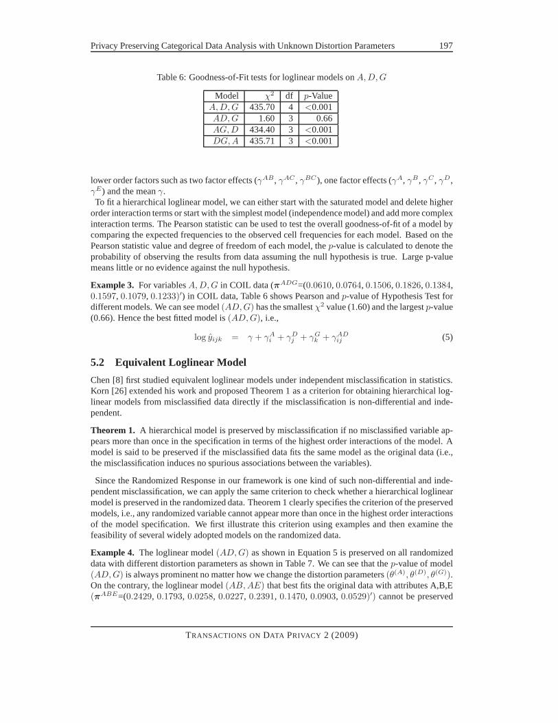
Table 6: Goodness-of-Fit tests for loglinear models onA, D, G

Model χ2 df p-ValueA, D, G 435.70 4 <0.001AD, G 1.60 3 0.66AG, D 434.40 3 <0.001DG, A 435.71 3 <0.001

lower order factors such as two factor effects (γAB, γAC , γBC ), one factor effects (γA, γB, γC , γD,γE) and the meanγ.To fit a hierarchical loglinear model, we can either start with the saturated model and delete higher

order interaction terms or start with the simplest model (independence model) and add more complexinteraction terms. The Pearson statistic can be used to testthe overall goodness-of-fit of a model bycomparing the expected frequencies to the observed cell frequencies for each model. Based on thePearson statistic value and degree of freedom of each model,thep-value is calculated to denote theprobability of observing the results from data assuming thenull hypothesis is true. Large p-valuemeans little or no evidence against the null hypothesis.

Example 3. For variablesA, D, G in COIL data (πADG=(0.0610, 0.0764, 0.1506, 0.1826, 0.1384,0.1597, 0.1079, 0.1233)′) in COIL data, Table 6 shows Pearson andp-value of Hypothesis Test fordifferent models. We can see model(AD, G) has the smallestχ2 value (1.60) and the largestp-value(0.66). Hence the best fitted model is(AD, G), i.e.,

log yijk = γ + γAi + γD

j + γGk + γAD

ij (5)

5.2 Equivalent Loglinear Model

Chen [8] first studied equivalent loglinear models under independent misclassification in statistics.Korn [26] extended his work and proposed Theorem 1 as a criterion for obtaining hierarchical log-linear models from misclassified data directly if the misclassification is non-differential and inde-pendent.

Theorem 1. A hierarchical model is preserved by misclassification if nomisclassified variable ap-pears more than once in the specification in terms of the highest order interactions of the model. Amodel is said to be preserved if the misclassified data fits thesame model as the original data (i.e.,the misclassification induces no spurious associations between the variables).

Since the Randomized Response in our framework is one kind ofsuch non-differential and inde-pendent misclassification, we can apply the same criterion to check whether a hierarchical loglinearmodel is preserved in the randomized data. Theorem 1 clearlyspecifies the criterion of the preservedmodels, i.e., any randomized variable cannot appear more than once in the highest order interactionsof the model specification. We first illustrate this criterion using examples and then examine thefeasibility of several widely adopted models on the randomized data.

Example 4. The loglinear model(AD, G) as shown in Equation 5 is preserved on all randomizeddata with different distortion parameters as shown in Table7. We can see that thep-value of model(AD, G) is always prominent no matter how we change the distortion parameters(θ(A), θ(D), θ(G)).On the contrary, the loglinear model(AB, AE) that best fits the original data with attributes A,B,E(πABE=(0.2429, 0.1793, 0.0258, 0.0227, 0.2391, 0.1470, 0.0903, 0.0529)′) cannot be preserved



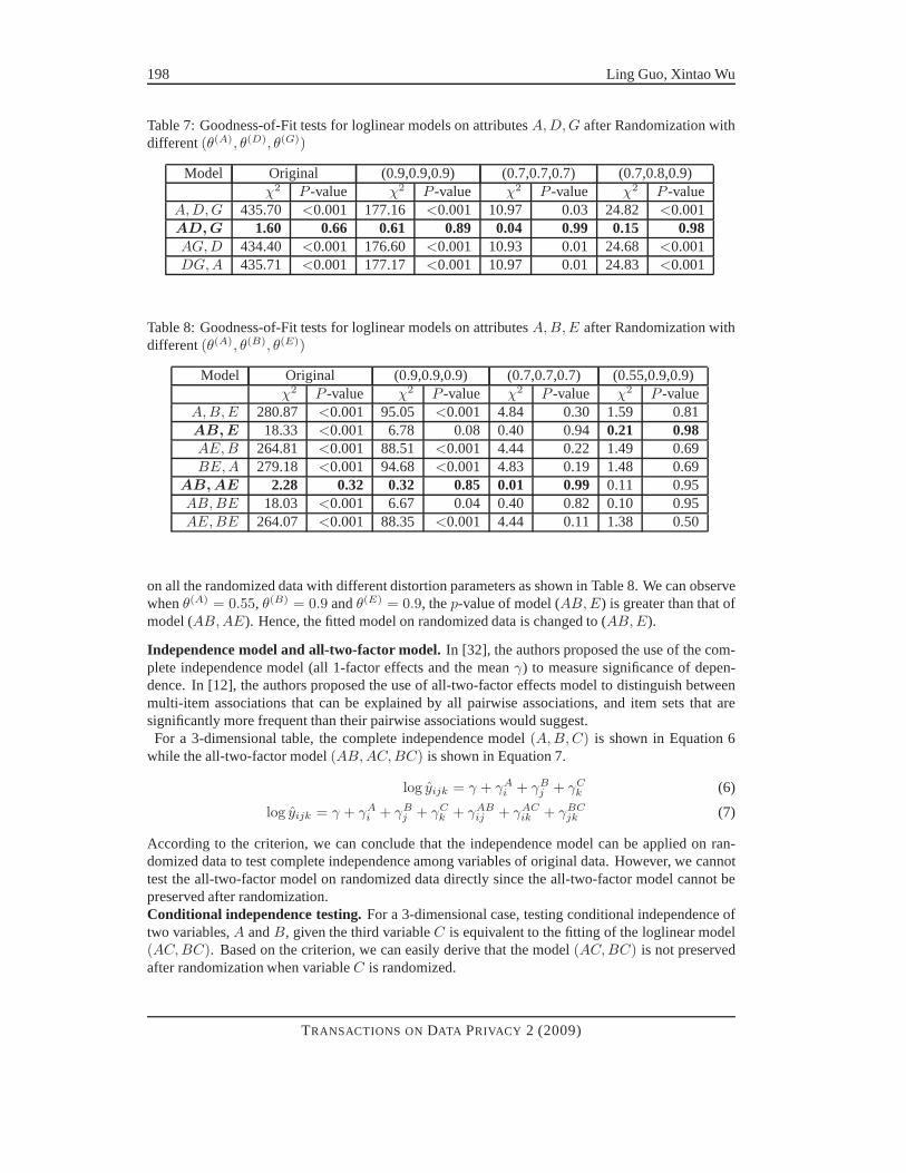
Table 7: Goodness-of-Fit tests for loglinear models on attributesA, D, G after Randomization withdifferent(θ(A), θ(D), θ(G))

Model Original (0.9,0.9,0.9) (0.7,0.7,0.7) (0.7,0.8,0.9)χ2 P -value χ2 P -value χ2 P -value χ2 P -value

A, D, G 435.70 <0.001 177.16 <0.001 10.97 0.03 24.82 <0.001AD, G 1.60 0.66 0.61 0.89 0.04 0.99 0.15 0.98AG, D 434.40 <0.001 176.60 <0.001 10.93 0.01 24.68 <0.001DG, A 435.71 <0.001 177.17 <0.001 10.97 0.01 24.83 <0.001

Table 8: Goodness-of-Fit tests for loglinear models on attributesA, B, E after Randomization withdifferent(θ(A), θ(B), θ(E))

Model Original (0.9,0.9,0.9) (0.7,0.7,0.7) (0.55,0.9,0.9)χ2 P -value χ2 P -value χ2 P -value χ2 P -value

A, B, E 280.87 <0.001 95.05 <0.001 4.84 0.30 1.59 0.81AB, E 18.33 <0.001 6.78 0.08 0.40 0.94 0.21 0.98AE, B 264.81 <0.001 88.51 <0.001 4.44 0.22 1.49 0.69BE, A 279.18 <0.001 94.68 <0.001 4.83 0.19 1.48 0.69

AB, AE 2.28 0.32 0.32 0.85 0.01 0.99 0.11 0.95AB, BE 18.03 <0.001 6.67 0.04 0.40 0.82 0.10 0.95AE, BE 264.07 <0.001 88.35 <0.001 4.44 0.11 1.38 0.50

on all the randomized data with different distortion parameters as shown in Table 8. We can observewhenθ(A) = 0.55, θ(B) = 0.9 andθ(E) = 0.9, thep-value of model (AB, E) is greater than that ofmodel (AB, AE). Hence, the fitted model on randomized data is changed to (AB, E).

Independence model and all-two-factor model.In [32], the authors proposed the use of the com-plete independence model (all 1-factor effects and the meanγ) to measure significance of depen-dence. In [12], the authors proposed the use of all-two-factor effects model to distinguish betweenmulti-item associations that can be explained by all pairwise associations, and item sets that aresignificantly more frequent than their pairwise associations would suggest.For a 3-dimensional table, the complete independence model(A, B, C) is shown in Equation 6

while the all-two-factor model(AB, AC, BC) is shown in Equation 7.


j + γCk (6)


j + γCk + γAB

ij + γACik + γBC

jk (7)

According to the criterion, we can conclude that the independence model can be applied on ran-domized data to test complete independence among variablesof original data. However, we cannottest the all-two-factor model on randomized data directly since the all-two-factor model cannot bepreserved after randomization.Conditional independence testing.For a 3-dimensional case, testing conditional independence oftwo variables,A andB, given the third variableC is equivalent to the fitting of the loglinear model(AC, BC). Based on the criterion, we can easily derive that the model(AC, BC) is not preservedafter randomization when variableC is randomized.



In practice, thepartial correlationis often adopted to measure the correlation between two variablesafter the common effects of all other variables in the data set are removed.

prAB.C =rAB − rACrBC

√

(1 − r2AC)(1 − r2

BC)(8)

Equation 8 shows the form for the partial correlation of two variables,A andB, while controllingfor a third variableC, whererAB denotes Pearson’s correlation coefficient. If there is no differencebetweenprAB.C and rAB , we can infer that the control variableC has no effect. If the partialcorrelation approaches zero, the inference is that the original correlation is spurious (i.e., there isno direct causal link between the two original variables because the control variable is either thecommon anteceding cause, or the intervening variable).According to the criterion, we have the following results.

Result 7. Theχ2 test of the independence on two randomized variablesAu with Av (or onAu withBl) conditional on a set of variablesG (G ⊆ I) is a correctα-level test for independence onAu withAv (or Au with Bl) conditional onG while with reduced power if and only if no distorted sensitivevariable is contained inG.

Result 8. The partial correlation of two sensitive variables or the partial correlation of one sensitivevariable and one non-sensitive variable conditional on a set of variablesG (G ⊆ I) has monotonicproperty|prran| ≤ |prori| if and only if no distorted sensitive variable is contained in G.

Other association measures for multi variables.There are five measures (IS, I, PS, G2, χ2) thatcan be extended to multiple variables. Association measures for multiple variables need an assumedmodel (usually the complete independence model). We have shown thatG2 andχ2 on the indepen-dence model have monotonic relations. However, we can easily check thatIS, I, PS do not havemonotonic properties since they are determined by the difference between one cell entry value andits estimate from the assumed model. On the contrary,G2 andχ2 are aggregate measures which aredetermined by differences across all cell entries.

5.3 Variation of Loglinear Model Parameters

Parameters of loglinear models indicate the interactions between variables. For example, theγABij

is two-factor effect which shows the dependency within the distributions of the associated variablesA, B. We present our result below and leave detailed proof in Appendix.

Result 9. For anyk-factor coefficientγGk

(ir |dr∈Gk) in hierarchical loglinear model, no vertical mono-tonic property or horizontal relative order invariant property is held after randomization.

6 Effects on Other Data Mining Applications

In this section, we examine whether some classic data miningtasks can be conducted on randomizeddata directly.

6.1 Association Rule Mining

Association rule learning is a widely used method for discovering interesting relations between itemsin data mining [2]. An association ruleX ⇒ Y, whereX ,Y ⊂ I andX ∩Y = φ, has two measures:the supports defined ass(100%) of the transactions inT that containX ∪ Y, and the confidencec is defined asc(100%) of the transactions inT that containX also containY. From Result 1 and



Result 2, we can easily learn that neither support nor confidence measures of association rule miningholds monotonic relations. Hence, we cannot conduct association rule mining on randomized datadirectly since values of support and confidence can become greater or less than the original onesafter randomization.

6.2 Decision Tree Learning

Decision tree learning is a procedure to determine the classof a given instance [30]. Several mea-sures have been used in selecting attributes for classification. Among them, gini function measuresthe impurity of an attribute with respect to the classes. If a data setD contains examples fromlclasses, given the probabilities for each class (pi), gini(D) is defined asgini(D) = 1 −

∑li=1 p2

i .WhenD is split into two subsetsD1 andD2 with sizesn1 andn2 respectively, the gini index of

the split data is:

ginisplit(D) =n1

ngini(D1) +

n2

ngini(D2)

The attribute with the smallestginisplit(D) is chosen to split the data.

Result 10. The relative order of gini values can not be preserved after randomization. That is, thereis no guarantee that the same decision tree can be learned from the randomized data.

Example 5. For variablesA,B,C (πABC=(0.2406,0.1815, 0.0453, 0.0031,0.3458, 0.0404,0.1431,0.0002)′) in COIL data, we setA,B as two sensitive attributes andC as class attribute. Theginivalues ofA, B before randomization are:

ginisplit(A)ori = πAgini(A1) + πAgini(A2)

= πA[1 − (πAC

πA

)2 − (πAC

πA

)2] + πA[1 − (πAC

πA)2 − (

πAC

πA)2]

= 0.30

Similarly, ginisplit(B)ori = 0.33.

After randomization with distortion parametersθ(A)0 = θ

(A)1 = 0.6 and θ

(B)0 = θ

(B)1 = 0.9

(λABC=(0.2629, 0.1127, 0.1042, 0.0143, 0.2837, 0.0873, 0.1240, 0.0109)′), we get:

ginisplit(A)ran = 0.35 ginisplit(B)ran = 0.34

The relative order ofginisplit(A) andginisplit(B) can not be preserved after randomization.

6.3 Naıve Bayes Classifier

A naıve Bayes classifier is a probabilistic classifier to predict the class label for a given instancewith attributes setX . It is based on applying Bayes’ theorem (from Bayesian statistics) with strongassumptions that the attributes are conditional independence given class labelC .Given an instance with feature vectorx, the naıve Bayes classifier to determine its class labelC is

defined as:

h∗(x) = argmaxiP (X = x|C = i)P (C = i)

P (X = x)

It chooses the maximum a posteriori probability (MAP) hypothesis to classify the example.



Result 11. The relative order of posteriori probabilities can not be preserved after randomization.That is, instances can not be classified correctly based on the Naıve Bayes classifier derived fromrandomized data directly.

Example 6. For variablesA,G,H (πAGH=(0.1884 , 0.0232,0.0802,0.1788,0.2264,0.0199, 0.1031,0.1800)′) in COIL data, we setA,G as two sensitive attributes andH as class attribute. For an in-stance with attributesA = 0, G = 1, the probability of its classH = 0 before randomizationis:

P (H |AG)ori = P (A|H) × P (G|H) × P (H)/P (AG)

=πAH

πH

× πGH

πH

× πH/πAG

=πAHπGH

πH

/πAG

= 0.31

Similarly, the probability of its classH = 1 is:

P (H |AG)ori =πAHπGH

πH/πAG = 0.69

After randomization with distortion parametersθ(A)0 =θ

(A)1 =θ

(G)0 =θ

(G)1 = 0.6 (λAGH=(0.1579,0.0848,

0.1351, 0.1163, 0.1643, 0.0845, 0.1408,0.1162)′), we get:

P (H|AG)ran = 0.54 P (H |AG)ran = 0.46

As none ofπAH , πGH , πAH , πGH has monotonic properties after randomization, the relative orderof the two probabilitiesP (H |AG) andP (H |AG) cannot be kept.

7 Conclusion

The trade-off between privacy preservation and utility loss has been extensively studied in privacypreserving data mining. However, data owners are still reluctant to release their (perturbed or trans-formed) data due to privacy concerns. In this paper, we focuson the scenario where distortionparameters are not disclosed to data miners and investigatewhether data mining or statistical anal-ysis tasks can still be conducted on randomized categoricaldata. We have examined how variousobjective association measures between two variables may be affected by randomization. We thenextended to multiple variables by examining the feasibility of hierarchical loglinear modeling. Wehave shown that some classic data mining tasks (e.g., association rule mining, decision tree learning,naıve Bayes classifier) cannot be applied on the randomizeddata with unknown distortion param-eters. We provided a reference to data miners about what theycan do and what they can not dowith certainty upon randomized data directly without the knowledge about the original distributionof data and distortion information.In our future work, we will comprehensively examine variousdata mining tasks (e.g., causal learn-

ing) as well as their associated measures in detail. We will conduct experiments on large data sets toevaluate how strong our theoretical results may hold in practice. We are also interested in extendingthis study to numerical data or networked data.

Acknowledgment

This work was supported in part by U.S. National Science Foundation IIS-0546027.



References

[1] D. Agrawal and C. C. Aggarwal. On the design and quantification of privacy preserving data miningalgorithms. InProceedings of the 20th Symposium on Principles of DatabaseSystems, 2001.

[2] R. Agrawal, T. Imielinski, and A. Swami. Mining association rules between sets of items in largedatabases. InSIGMOD Conference, pages 207–216, 1993.

[3] R. Agrawal and R. Srikant. Privacy-preserving data mining. In Proceedings of the ACM SIGMODInternational Conference on Management of Data, pages 439–450. Dallas, Texas, May 2000.

[4] S. Agrawal and J. R. Haritsa. A framework for high-accuracy privacy-preserving mining. InProceedingsof the 21st IEEE International Conference on Data Engineering, pages 193–204, 2005.

[5] A. Agresti. Categorical data analysis. Wiley, 2002.

[6] R. Brand. Microdata protection through noise addition.Lecture Notes in Computer Science, 2316:97–116, 2002.

[7] A. Chaudhuri and R. Mukerjee.Randomized response: theory and techniques. Marcel Dekker, 1988.

[8] T. T. Chen. Analysis of randomized response as purposively misclassified data.Journal of the AmericanStatistical Association, pages 158–163, 1979.

[9] J. Domingo-Ferrer, J.M. Mateo-Sanz, and V. Torra. Comparing SDC methods for micro-data on the basisof information loss and disclosure risk. InProceedings of NTTS and ETK, 2001.

[10] W. Du, Z. Teng, and Z. Zhu. Privacy-maxent: integratingbackground knowledge in privacy quantifi-cation. InProceedings of the ACM SIGMOD International Conference on Management of Data, pages459–472, 2008.

[11] W. Du and Z. Zhan. Using randomized response techniquesfor privacy-preserving data mining. InPro-ceedings of the 9th ACM SIGKDD International Conference on Knowledge Discovery and Data Mining,pages 505–510, 2003.

[12] W. DuMouchel and D. Pregibon. Empirical bayes screening for multi-item association. InProceedingsof the ACM SIGKDD Conference on Knowledge Discovery and DataMining. San Francisco, CA, August2001.

[13] A. Evfimievski. Randomization in privacy preserving data mining.ACM SIGKDD Explorations Newslet-ter, 4(2):43–48, 2002.

[14] A. Evfimievski, J. Gehrke, and R. Srikant. Limiting privacy breaches in privacy preserving data min-ing. In Proceedings of the 22nd ACM SIGACT-SIGMOD-SIGART Symposium on Principles of DatabaseSystems, pages 211–222, 2003.

[15] A. Evfimievski, R. Srikant, R. Agrawal, and J. Gehrke. Privacy preserving mining of association rules.Proceedings of the 8th ACM SIGKDD International Conferenceon Knowledge Discovery and Data Min-ing, pages 217–228, 2002.

[16] L. Geng and H. J. Hamilton. Interestingness measures for data mining: A survey .ACM ComputingSurveys, 38(3):9, 2006.

[17] S. Gomatam and A. F. Karr. Distortion measures for categorical data swapping. Technical Report,Number 131, National Institute of Statistical Sciences, 2003.

[18] J. M. Gouweleeuw, P. Kooiman, L. C. R. J. Willenborg, andP. P. de Wolf. Post randomization forstatistical disclosure control: theory and implementation. Journal of Official Statistics, 14(4):463–478,1998.

[19] L. Guo, S. Guo, and X. Wu. Privacy preserving market basket data analysis. InProceedings of the11th European Conference on Principles and Practice of Knowledge Discovery in Databases, September2007.

[20] L. Guo, S. Guo, and X. Wu. On addressing accuracy concerns in privacy and preserving association rulemining. InProceedings of the 12th Pacific-Asia Conference on Knowledge Discovery and Data Mining,May 2008.



[21] M. Hay, G. Miklau, D. Jensen, P. Weis, and S. Srivastava.Anonymizing social networks.TechnicalReport, University of Massachusetts, 07-19, 2007.

[22] Z. Huang and W. Du. Optrr: Optimizing randomized response schemes for privacy-preserving datamining. InProceedings of the 24th IEEE International Conference on Data Engineering, pages 705–714,2008.

[23] Z. Huang, W. Du, and B. Chen. Deriving private information from randomized data. InProceedings ofthe ACM SIGMOD Conference on Management of Data. Baltimore, MA, 2005.

[24] H. Kargupta, S. Datta, Q. Wang, and K. Sivakumar. On the privacy preserving properties of randomdata perturbation techniques. InProceedings of the 3rd International Conference on Data Mining, pages99–106, 2003.

[25] J. Kim. A method for limiting disclosure in microdata based on random noise and transformation. InProceedings of the American Statistical Association on Survey Research Methods, 1986.

[26] E. L. Korn. Hierarchical log-linear models not preserved by classification error.Journal of the AmericanStatistical Association, 76:110–113, 1981.

[27] K. Liu and E. Terzi. Towards identity anonymization on graphs. InProceedings of the ACM SIGMODConference, Vancouver, Canada, 2008. ACM Press.

[28] D. J. Martin, D. Kifer, A. Machanavajjhala, J. Gehrke, and J. Y. Halpern. Worst-case background knowl-edge in privacy. Technical Report, Cornell University, 2006.

[29] G. Piatetsky-Shapiro. Discovery, analysis, and presentation of strong rules.Knowledge Discovery inDatabases, pages 229–248, 1991.

[30] J. R. Quinlan.C4.5: programs for machine learning. Morgan Kaufmann Publishers Inc., San Francisco,CA, USA, 1993.

[31] S. J. Rizvi and J. R. Haritsa. Maintaining data privacy in association rule mining. InProceedings of the28th International Conference on Very Large Data Bases, 2002.

[32] C. Silverstein, S. Brin, and R. Motwani. Beyond market baskets: generalizing association rules to depen-dence rules.Data Mining and Knowledge Discovery, 2:39–68, 1998.

[33] P. Tan, V. Kumar, and J. Srivastava. Selecting the rightinterestingness measure for association patterns.In Proceedings of the 8th International Conference on Knowledge Discovery and Data Mining, pages32–41, 2002.

[34] P. Tan, M. Steinbach, and K. Kumar.Introduction to data mining. Addison Wesley, 2006.

[35] A. Van den Hot. Analyzing misclassified data: randomized response and post randomization. Ph.D.Thesis, University of Utrecht, 2004.

[36] L. Willenborg and T. De Waal. Elements of statistical disclosure control in practice.Lecture Notes inStatistics, 155, 2001.

[37] X. Ying and X. Wu. Randomizing social networks: a spectrum preserving approach. InProceedings ofthe 8th SIAM Conference on Data Mining, April 2008.

A Proof of Results

Proof of Result 1 and Result 2The Added Value calculated directly from the randomized data without knowingPu, Pv is

AVran =λ11

λ1+− λ+1 =

λ11 − λ+1λ1+

λ1+

The original Added Value can be expressed as

AVori =π11 − π+1π1+

π1+



As π = (P−1u × P−1

v )λ, we have:

π1+ =θ(u)1 − 1 + (1 + θ

(u)0 − θ

(u)1 )λ1+

θ(u)0 + θ

(u)1 − 1

π+1 =θ(v)1 − 1 + (1 + θ

(v)0 − θ

(v)1 )λ+1

θ(v)0 + θ

(v)1 − 1

π11 − π+1π1+ =λ11 − λ+1λ1+

(θ(u)0 + θ

(u)1 − 1)(θ

(v)0 + θ

(v)1 − 1)

Through deduction,AVori is expressed as:

AVori =λ11 − λ+1λ1+

(θ(v)0 + θ

(v)1 − 1)[θ

(u)1 − 1 + (1 + θ

(u)0 − θ

(u)1 )λ1+]

Let f(θ(u)0 , θ

(u)1 , θ

(v)0 , θ

(v)1 , λ1+) = |(θ(v)

0 + θ(v)1 − 1)[θ

(u)1 − 1 + (1 + θ

(u)0 − θ

(u)1 )λ1+]| − |λ1+|,

1) Whenθ(u)0 , θ

(u)1 , θ

(v)0 , θ

(v)1 ∈ [0.5, 1], sinceπ1+ =

θ(u)1 −1+(1+θ

(u)0 −θ

(u)1 )λ1+

θ(u)0 +θ

(u)1 −1

≥ 0, thenθ(u)1 −1+

(1 + θ(u)0 − θ

(u)1 )λ1+ ≥ 0, we have

f(θ(u)0 , θ

(u)1 , θ

(v)0 , θ

(v)1 , λ1+) = (θ

(v)0 + θ

(v)1 − 1)[θ

(u)1 − 1 + (1 + θ

(u)0 − θ

(u)1 )λ1+] − λ1+

= (θ(v)0 + θ

(v)1 − 1)(θ

(u)1 − 1)(1 − λ1+) + [(θ

(v)0 + θ

(v)1 − 1)θ

(u)0 − 1]λ1+

≤ 0

Hence,

|AVori| = | λ11 − λ+1λ1+

(θ(v)0 + θ

(v)1 − 1)[θ

(u)1 − 1 + (1 + θ

(u)0 − θ

(u)1 )λ1+]

|

≥ |λ11 − λ+1λ1+

λ1+|

≥ |AVran|

2) Whenθ(u)0 , θ

(u)1 , θ

(v)0 , θ

(v)1 ∈ [0, 0.5], sinceθ

(u)1 − 1 + (1 + θ

(u)0 − θ

(u)1 )λ1+ ≥ 0, we have

f(θ(u)0 , θ

(u)1 , θ

(v)0 , θ

(v)1 , λ1+) = (θ

(v)0 + θ

(v)1 − 1)(θ

(u)1 − 1)(1 − λ1+) + [(θ

(v)0 + θ

(v)1 − 1)θ

(u)0 − 1]λ1+

whenλ1+ ≥ (θ(v)0 +θ

(v)1 −1)(θ

(u)1 −1)

1−(θ(u)0 +θ

(v)1 −1)(1+θ

(u)0 −θ

(u)1 )

f(θ(u)0 , θ

(u)1 , θ

(v)0 , θ

(v)1 , λ1+) ≤ 0, |AVori| ≥ |AVran|

whenλ1+ <(θ

(v)0 +θ

(v)1 −1)(θ

(u)1 −1)

1−(θ(v)0 +θ

(v)1 −1)(1+θ

(u)0 −θ

(u)1 )

f(θ(u)0 , θ

(u)1 , θ

(v)0 , θ

(v)1 , λ1+) > 0, |AVori| < |AVran|

Similarly, we can prove that|AVori| ≥ |AVran| is not always held whenθ(u)0 , θ

(u)1 , θ

(v)0 , θ

(v)1 /∈

[0.5, 1].Proof of Result 3 and Result 4



For any pair of variables, Piatetsky-Shapiro’s measure calculated directly from the randomized datawithout knowingθ

(u)0 , θ

(u)1 , θ

(v)0 , θ

(v)1 is:

PSran = λ11 − λ1+λ+1 = λ00λ11 − λ01λ10

The original Piatetsky-Shapiro’s measure is:

PSori = π11 − π1+π+1 =PSran

(θ(u)0 + θ

(u)1 − 1)(θ

(v)0 + θ

(v)1 − 1)

|PSu,vori | − |PSs,t

ori| =|PSu,v

ran| − |PSs,tran|

|(θ(u)0 + θ

(u)1 − 1)(θ

(v)0 + θ

(v)1 − 1)|

So∀θ(u)0 , θ

(u)1 , θ

(v)0 , θ

(v)1 ∈ [0, 1], 1

|(θ(u)0 +θ

(u)1 −1)(θ

(v)0 +θ

(v)1 −1)|

≥ 1. Result 3 is proved.

Since

Dran =λ00

λ+0− λ01

λ+1=

λ00λ11 − λ01λ10

λ+0λ+1

Dori =π00π11 − π01π10

π+0π+1=

λ00λ11 − λ01λ10

(θ(u)0 + θ

(u)1 − 1)λ+0λ+1

We haveDori = 1

(θ(u)0 +θ

(u)1 −1)

Dran. Hence,

|Du,sori| − |Dv,t

ori| =1

|θ(u)0 + θ

(u)1 − 1|

(|Du,sran| − |Dv,t

ran|)

We can showAV also holds. Result 4 is proved.Proof of Result 9The proof is given for three binary variables with the saturated model; the extension to higher di-

mensions is immediate. Equation 9 shows how to compute the coefficients for the model of variablesA, B, C, where a dot “.” means that the parameter has been summed overthe index.

γ = l...

γAi = li.. − γ

· · ·γAB

ij = lij. − γAi − γB

j − γ

· · ·γABC

ijk = lijk − γABij − γAC

ik − γBCjk − γA

i − γBj − γC

k − γ

(9)

From randomized data we get:

γA0ran =

1

8log

λ000λ001λ010λ011

λ100λ101λ110λ111

Similarly, we have:

γA0ori =

1

8log

π000π001π010π011

π100π101π110π111

There is no monotonic relation betweenλijk andπijk (i, j, k = 0, 1). γA can be greater or less thanthe original value after randomization. Same results can beproved for otherγ parameters. Result 9is proved.


privacy preserving categorical data analysis with unknown ... · transactions on data privacy 2...

Documents