Privacy Preserving Techniques for Speech Processing

Manas A. Pathak

December 1, 2010

Language Technologies InstituteSchool of Computer ScienceCarnegie Mellon University

Pittsburgh, PA 15213

Thesis CommitteeBhiksha Raj (chair)

Alan BlackAnupam Datta

Paris Smaragdis, UIUCShantanu Rane, MERL

PhD Thesis Proposal

Copyright c© 2010 Manas A. Pathak

2

Abstract

Speech is perhaps the most private form of personal communication but current speech processing techniques are notdesigned to preserve the privacy of the speaker and require complete access to the speech recording. We propose todevelop techniques for speech processing which do preserve privacy. While our proposed methods can be applied to avariety of speech processing problems and also generally to problems in other domains, we focus on the problems ofkeyword spotting, speaker identification, speaker verification, and speech recognition.

Each of these applications involve the two separate but overlapping problems of private classifier evaluation andprivate classifier release. Towards the former, we study designing privacy preserving protocols using primitives such ashomomorphic encryption, oblivious transfer, and blind and permute in the framework of secure multiparty computation(SMC). Towards the latter, we study the differential privacy model, and techniques such as exponential method andsensitivity method for releasing differentially private classifiers trained on private data.

We summarize our preliminary work on the subject including techniques such as SMC protocols for eigenvectorcomputation, isolated keyword recognition and differentially private release mechanisms for large margin Gaussianmixture models, and classifiers trained from data belonging to multiple parties. Finally, we discuss the proposed direc-tions of research including techniques such as training differentially private hidden Markov models, and a multipartyframework for differentially private classification by data perturbation, and protocols for applications such as privacypreserving music matching and keyword spotting, speaker verification and identification.

3

4

Contents

1 Introduction 71.1 Outline . . . . . . . . . . . . . . . . . . . . . . . . . . . . . . . . . . . . . . . . . . . . . . . . . . 8

2 Speech Applications and Privacy 92.1 Basic Tools . . . . . . . . . . . . . . . . . . . . . . . . . . . . . . . . . . . . . . . . . . . . . . . . 9

2.1.1 Signal Parameterization . . . . . . . . . . . . . . . . . . . . . . . . . . . . . . . . . . . . . 92.1.2 Gaussian Mixture Models . . . . . . . . . . . . . . . . . . . . . . . . . . . . . . . . . . . . 102.1.3 Hidden Markov Models . . . . . . . . . . . . . . . . . . . . . . . . . . . . . . . . . . . . . 10

2.2 Speech Processing Applications . . . . . . . . . . . . . . . . . . . . . . . . . . . . . . . . . . . . . 102.2.1 Speaker Verification and Identification . . . . . . . . . . . . . . . . . . . . . . . . . . . . . . 112.2.2 Music Matching . . . . . . . . . . . . . . . . . . . . . . . . . . . . . . . . . . . . . . . . . 122.2.3 Keyword Spotting . . . . . . . . . . . . . . . . . . . . . . . . . . . . . . . . . . . . . . . . 132.2.4 Speech Recognition . . . . . . . . . . . . . . . . . . . . . . . . . . . . . . . . . . . . . . . 14

3 Background on Privacy and Security 173.1 Secure Multiparty Computation . . . . . . . . . . . . . . . . . . . . . . . . . . . . . . . . . . . . . 17

3.1.1 Data Setup and Privacy Conditions . . . . . . . . . . . . . . . . . . . . . . . . . . . . . . . . 173.1.2 Tools for Constructing SMC protocols . . . . . . . . . . . . . . . . . . . . . . . . . . . . . . 183.1.3 Related Work on SMC Protocols for Machine Learning and Speech Processing . . . . . . . . 19

3.2 Differential Privacy . . . . . . . . . . . . . . . . . . . . . . . . . . . . . . . . . . . . . . . . . . . . 193.2.1 Related Work on Differentially Private Machine Learning . . . . . . . . . . . . . . . . . . . 19

4 Preliminary Work 214.1 Techniques . . . . . . . . . . . . . . . . . . . . . . . . . . . . . . . . . . . . . . . . . . . . . . . . 21

4.1.1 Privacy Preserving Eigenvector Computation . . . . . . . . . . . . . . . . . . . . . . . . . . 214.1.2 Differentially Private Large Margin Gaussian Mixture Models . . . . . . . . . . . . . . . . . 264.1.3 Differentially Private Classification from Multiparty Data . . . . . . . . . . . . . . . . . . . 30

4.2 Applications . . . . . . . . . . . . . . . . . . . . . . . . . . . . . . . . . . . . . . . . . . . . . . . . 344.2.1 Privacy Preserving Keyword Recognition . . . . . . . . . . . . . . . . . . . . . . . . . . . . 344.2.2 A framework for implementing SMC protocols . . . . . . . . . . . . . . . . . . . . . . . . . 39

5 Proposed Work 415.1 Techniques . . . . . . . . . . . . . . . . . . . . . . . . . . . . . . . . . . . . . . . . . . . . . . . . 41

5.1.1 Differentially Private Hidden Markov Models . . . . . . . . . . . . . . . . . . . . . . . . . . 415.1.2 Differential Private Classification by Transforming the Loss Function . . . . . . . . . . . . . 415.1.3 Optional: Privately Training Classifiers over Data from Different Distributions . . . . . . . . 42

5.2 Applications . . . . . . . . . . . . . . . . . . . . . . . . . . . . . . . . . . . . . . . . . . . . . . . . 425.2.1 Privacy Preserving Music Recognition and Keyword Spotting . . . . . . . . . . . . . . . . . 425.2.2 Privacy Preserving Speaker Verification and Identification . . . . . . . . . . . . . . . . . . . 425.2.3 Optional: Privacy Preserving Graph Search for Speech Recognition . . . . . . . . . . . . . . 43

5.3 Estimated Timeline . . . . . . . . . . . . . . . . . . . . . . . . . . . . . . . . . . . . . . . . . . . . 43

5

A Proofs of Theorems and Lemmas 49A.1 Privacy Preserving Eigenvector Computation (Section 4.1.1) . . . . . . . . . . . . . . . . . . . . . . 49A.2 Differentially Private Large Margin Gaussian Mixture Models (Section 4.1.2) . . . . . . . . . . . . . 49A.3 Differentially Private Classification from Multiparty Data (Section 4.1.3) . . . . . . . . . . . . . . . . 52

6

Chapter 1

Introduction

Speech is perhaps the most private form of personal communication. A sample of a person’s voice contains informationnot only about the message but also about the person’s gender, accent, nationality, the emotional state. Therefore,no one would like to have their voice being recorded without consent through eavesdropping or wiretaps – in fact,such activities are considered illegal in most situations. Yet, current speech processing techniques such as speakeridentification, speech recognition are not designed to preserve the privacy of the speaker and require complete accessto the speech recording.

We propose to develop privacy-preserving techniques for speech processing. There have been privacy preservingtechniques proposed for a variety of learning and classification tasks, such as multiple parties performing decisiontrees [Vaidya et al., 2008a], clustering [Lin et al., 2005], association rule mining [Kantarcioglu and Clifton, 2004],naive Bayes classification [Vaidya et al., 2008b], support vector machines [Vaidya et al., 2008c] and rudimentary com-puter vision applications [Avidan and Butman, 2006], but there has been little work on techniques for privacy preserv-ing speech processing. While our proposed techniques can be applied to a variety of speech processing problems andalso generally to problems in other domains, we focus on the following problems where we believe privacy-preservingsolutions are of direct interest.

1. Keyword spotting. Keyword spotting systems detect if a specified keyword has occurred in a recording. Itis therefore useful if the the system can detect only the presence of the keyword without having access to thespeech recording. Such a system would find applications in surveillance applications and pass-phrase detection.It would also enable privacy preserving speech mining applications for extracting statistics about the occurrenceof specific keywords in an collection of recordings, while not learning anything else about the speech data.

2. Speaker Identification. Speaker identification systems attempt to identify which, if any, of a specified set ofspeakers has spoken into the system. In many situations, it would be useful to be permit speaker identificationwithout providing access to any other information in the voice. For instance, a security agency may be able todetect if a particular speaker has spoken in a phone conversation without being able to discover who else spokeor what was spoken in the audio.

3. Speaker Verification. Speaker verification systems determine if a speaker is indeed who the speaker claims tobe. Users may want the system not to have access to their voice and therefore the identity. In text-dependentverification systems, users may not want the system to be able to discover their pass-phrase.

4. Speech Recognition. Speech recognition is the problem of automatically transcribing the text from the speechrecording. While the use of cloud based online services has been prevalent for many tasks, the private nature ofspeech data is a major stumbling block towards creating such a speech recognition service. To overcome this,it is desirable to have a privacy preserving speech recognition system which can perform recognition withouthaving access to the speech data.

It should be noted that we are not developing new algorithms which achieve and extend the state of the art perfor-mance of the above applications. We are interested in creating privacy preserving frameworks for existing algorithms.

7

The proposed technology has broad implications not just in the area of speech processing, but to society at large.As voice technologies proliferate, people have increasing reason to distrust them. With increasing use of speech recog-nition based user interfaces, speaker verification based authentication systems, and automated systems for ubiquitousapplications, from routing calls to purchasing airline tickets, the ability of malicious entities to capture and misusea person’s voice has never been greater, and this threat is only expected to increase. The fallout of such misuse canpose a far greater threat than mere loss of privacy but have severe economic and social impacts as well. This proposalrepresents a proactive effort at developing technologies to secure voice processing systems to prevent such misuse.

1.1 OutlineWe first review the basics of speech processing in Chapter 2 and privacy in Chapter 3. Each of the problems mentionedabove broadly involves two separate but overlapping aspects: function computation – training and evaluation of clas-sifiers over private speech data and function release – publishing classifiers trained over private speech data. Towardsthe former problem, we investigate cryptographic protocols in the secure multiparty computation framework (Section3.1) and for the latter problem we investigate differentially private release mechanisms (Section 3.2). We discuss ourpreliminary work towards this direction in Chapter 4 and the proposed work in Chapter 5.

8

Chapter 2

Speech Applications and Privacy

We first review some of the basic building blocks used in speech processing systems. Almost all speech processingtechniques follow a two-step process of signal parameterization followed by classification. This is shown in Figure 2.1.

Speech Signal

Feature Computation

Features

Pattern Matching

Output

Acoustic Model

Language Model

Figure 2.1: Work flow of a speech processing system.

2.1 Basic Tools

2.1.1 Signal Parameterization

The most common parametrization for speech is the mel-frequency cepstral coefficients (MFCC) [Davis and Mermel-stein, 1980]. In this representation, we sample the speech signal at a high frequency and take the Fourier transformof each short time window. This is followed by de-correlating the spectrum using a cosine transform, then taking themost significant coefficients.

IfX is a vector of signal samples, F is the Fourier transform in matrix form, M is the set of Mel filters representedas a matrix, and D is a DCT matrix, MFCC feature vectors can be computed as D log(M((FX) · conjugate(FX))).

9

s1 s2 s3 s4 s5

x1 x2 x3 x4 x5

a12 a23 a34 a45

a54a43a32a21

a11 a22 a33 a44 a55

b1(x1) b2(x2) b3(x3) b4(x4) b5(x5)

Figure 2.2: An example of a 5-state HMM.

2.1.2 Gaussian Mixture ModelsGaussian mixture model (GMM) is a commonly used generative model for density estimation in speech and languageprocessing. The probability of each class generating an example is modeled as a mixture of Gaussian distributions.For problems such as speaker identification, we have one utterance x which we wish to classify by the class labelyi ∈ 1, . . . ,K representing a set of speakers. If the mean vector and covariance matrix of the jth Gaussian in theclass yi are µij and Σij , respectively, for an observation x, we have P (x|yi) =

∑j wijN (µij ,Σij), where wij are

the mixture coefficients. The above mentioned parameters can be computed using the expectation-maximization (EM)algorithm.

2.1.3 Hidden Markov ModelsA hidden Markov model (HMM) (Fig. 2.2), can be thought of as an example of a Markov model in which the state isnot directly visible but output of each state can be observed. The outputs are also referred to as observations. Sinceobservations depend on the hidden state, an observation reveals information about the underlying state.

A hidden Markov model is defined as a triple M = (A,B,Π), in which

• A = (aij) is the state transition matrix. Thus, aij = Pr{qt+1 = Sj |qt = Si}, 1 ≤ i, j ≤ N , where{S1, S2, ..., SN} is the set of states and qt is the state at time t.

• B = (bj(vk)) is the matrix containing the probabilities of the observations. Thus, bj(vk) = Pr{xt = vk|qt =Sj}, 1 ≤ j ≤ N, 1 ≤ k ≤M , where vk ∈ V which is the set of observation symbols, and xt is the observationat time t.

• Π = (π1, π2, ..., πN ) is the initial state probability vector, that is, πi = Pr{q1 = Si}, i = 1, 2, ..., N .

Depending on the set of observation symbols, we can classify HMMs into those with discrete outputs and thosewith continuous outputs. In speech processing applications, we consider HMMs with continuous outputs where eachthe observation probabilities of each state is modeled using a GMM. Such a model is typically used to model thesequential audio data frames representing the utterance of one word.

For a given sequence of observations x1,x2, ...,xT and an HMM λ = (A,B,Π), one problem of interest isto efficiently compute the probability P (x1,x2, ...,xT |λ). A well known solution to this problem is the forward-backward algorithm.

2.2 Speech Processing ApplicationsWe first introduce some terminology that we will employ in the rest of this document. The term speech processingrefers to pattern classification or learning tasks performed on voice data. A privacy preserving transaction is one whereno party learns anything about the others data. In the context of a speech processing system, this means that the systemdoes not learn anything about the user’s speech and the user does not learn anything of the internal parameters used by

10

the system. We often also refer to privacy-preserving operations as secure. We expand the conventional definition ofsystem to include the entity in charge of it who could log data and partial results for analysis. Current voice processingtechnologies are not designed to preserve the privacy of the speaker. Systems need complete access to the speechrecording which is usually in the parameterized form. The only privacy ensured is the loss of information effected bythe parametrization. Standard parametrizations can be inverted to obtain an intelligible speech signal and provide littleprotection of privacy. Yet, there are many situations in which voice processing needs to be performed while preservingthe privacy of subjects’ voices and processing may need to be performed without having access to the voice. Here, by“access to voice” we refer to having access to any form of the speech that can be converted to an intelligible signal, orfrom which information about the speaker or what was spoken could be determined.

There are three basic application areas where privacy preserving speech processing finds application.

1. Biometric Authentication.As a person’s voice is characteristic to the individual, speech is widely used in biometric authentication systems.This is also an important privacy concern for the user as the system always has access to the speech recording. Itis also possible for an adversary to break into the system to gain unauthorized access using pre-recorded voice.This can be prevented by using privacy preserving speaker verification.

2. Mining Speech Data.Corporations and call centers often have large quantities of voice data from which they may desire to detectpatterns. However, privacy concerns prevent them from providing access to external companies that can minethe data for patterns. Privacy preserving speaker identification and keyword spotting techniques can enable theoutside company to detect patterns without learning anything else about the data.

3. Recognition.Increasingly, speech recognition systems are deployed in a client server framework, where the client has theaudio recording and the server has a trained model. In this case, privacy is important as the server has completeaccess to the audio which is being used for recognition and is often the bottleneck in using such speech recogni-tion systems in contexts where the speech contains sensitive information. Similarly, it is also useful to developtechniques for training the model parameters.

The objective of our proposal is to develop privacy preserving techniques for some of the key voice processingtechnologies mentioned above. Specifically, we propose to develop privacy preserving techniques for speaker identi-fication, speaker verification, and keyword spotting. Note that our goal is not the development of more accurate andscalable speech processing algorithms; we focus will be to restructure the computations of current algorithms andembedding them within privacy frameworks such that the operations are preserve privacy. Where necessary, we willdevelop alternative algorithms or implementations that are inherently more amenable to having their computationsrestructured in this manner. We review the above mentioned speech processing applications along with the relevantprivacy issues.

2.2.1 Speaker Verification and IdentificationIn speaker verification, we try to ascertain if a user is who he or she claims to be. Speaker verification systems can betext dependent, where the speaker utters a specific pass phrase and the system verifies it by comparing the utterancewith the version recorded initially by the user. Alternatively, speaker verification can be text independent, where thespeaker is allowed to say anything and the system only determines if the given voice sample is close to the speaker’svoice. Speaker identification is a related problem in which we identify if a speech sample is spoken by any one ofthe speakers from our pre-defined set of speakers. The techniques employed in the two problems are very similar,enrollment data from each of the speakers are used to build statistical or discriminative models for the speaker whichare employed to recognize the class of a new audio recording.

Basic speaker verification and identification systems use a GMM classifier model trained over the voice of thespeaker. We typically use MFCC features of the audio data instead of the original samples as they are known to providebetter accuracy for speech classification. In case of speaker verification, we train a binary GMM classifier using the

11

audio samples of the speaker as one class and a universal background noise (UBM) model as another class [Campbell,2002]. UBM is trained over the combined speech data of all other users. Due to the sensitive nature of their use inauthentication systems, speaker verification classifiers need to be robust to false positives. In case of doubt about theauthenticity of a user, the system should choose to reject. In case of speaker identification, we also use the UBM tocategorize a speech sample as not being spoken by anyone from the set of speakers.

In practice, we need a lot of data from one speaker to train an accurate speaker classification model and suchdata is difficult to acquire. Towards this, Reynolds et al. [2000] proposed techniques for maximum a posterioriadaptation to derive speaker models from the UBM. These adaptation techniques have been extended by constructing“supervectors” consisting of the stacked means of the mixture components [Kenny and Dumouchel, 2004]. Thesupervector formulation has also been used with support vector machine (SVM) classification methods. Campbellet al. [2006] derive a linear kernel based upon an approximation to the KL divergence between the two GMM models.It might be noted that apart from the conventional generative GMM models, large margin GMMs [Sha and Saul, 2006]can also be used for speaker verification. A variety of other classification algorithms based on HMMs and SVMs havebeen proposed for speaker verification and speaker identification [Reynolds, 2002; Hatch and Stolcke, 2006].

Privacy Issues

There are different types of privacy requirements while performing speaker verification or identification in terms oftraining the classifier and evaluating a classifier.

1. Training. The basic privacy requirement here is that system should be able to train the speaker classificationmodel without being able to observe the speech data belonging to the users. This problem is an example ofsecure multiparty computation (Section 3.1), and protocols can be designed for this using primitives such ashomomorphic encryption. The UBM is trained over speech data acquired from different users. The individualcontribution of every user is private and the system should not have access to the speech recording. Additionally,even if the model is trained privately, the system should not be able to make any inference about the training databy analyzing the model. The differential privacy framework (Section 3.2) provides a probabilistic guarantee insuch a setting. This will allow the participants to share their data freely without any privacy implications.

In case of speaker verification, we need to train one classification model per speaker. In this case, the privacyrequirement is that the system should not know which model is currently being trained, i.e., it should not be ableto know the identity of any of speakers in the system.

2. Testing. Once the system has trained the model, we need to perform classification on new audio data. Here,the privacy requirement is that the system should not be able to observe the test data. Also, as the classificationmodel belonging to the system might be trained over valuable training data, it is not desirable for the systemto release the model parameters to the party with the test audio data. Finally, in both speaker verification andidentification, the system should be oblivious about the output of the classification. This problem is also anexample of secure multiparty computation and can be addressed using the appropriate primitives.

2.2.2 Music MatchingMusic matching falls under the broad category of music retrieval or audio mining applications. In a client-servermodel, we require to compare the input audio snippet of the client: Alice to a collection of longer audio recordingsbelonging to the server: Bob. Music matching involves finding an audio recording of a song from a central databasewhich most closely matches a given audio snippet. When a match is found, information about the song such as thetitle, artist, and album are transfered back to the user.

A simple algorithm to perform this matching is by computing the correlation between the music signals. Thismethod is fairly robust to noise in the snippets. Alternatively, if we are dealing with snippets which are also a copy ofthe original recording, we can directly compare a binary fingerprint of the snippet more efficiently. This technique isused in commercial systems such as [Wang, 2003]. To compare a short snippet to an audio recording of a song, weneed to perform a sliding window comparison for all samples of the recording, as shown in Figure 2.3. Bob needs tocompare every frame of every song in the collection with the snippet and choose the song with the highest score.

12

Song (Bob)

Snippet (Alice)

compare

Figure 2.3: Sliding window comparison of snippet frames and song frames.

Privacy Issues

Subsequently, if we need to perform music matching with privacy, our main requirement is that we need to do it withoutthe server observing the snippet provided by the client. Such a system would be very valuable in commercial as well asmilitary settings as discussed above. A trivial and completely impractical solution to this problem is that Bob sends hisentire music collection to Alice. Instead, we are interested in solutions in which Alice and Bob participate in a protocolwhich uses secure multiparty computation primitives (see Section 3.1) to perform the matching securely. Alice willgive to Bob an encryption of her audio snippet and Bob will be able to perform the matching operations privately andobtain all the sliding window scores in an encrypted form. Alice and Bob can then participate in an secure maximumfinding protocol to obtain the song with the highest score without the knowledge of Bob. Even doing this tends to becomputationally expensive, as it is performing operations on encrypted data is costly and still requires some amountof data transfer between Alice and Bob. In the secure protocol, we need to streamline the sliding window comparisonoperation. Another potential direction is to perform an efficient maximum finding algorithm which determines anapproximate maximum value by not making all the comparisons.

2.2.3 Keyword Spotting

Keyword spotting is a similar problem in which we try to find if one or more of a specified set of key words or phraseshas occurred in a recording. The main difference of this problem from music matching is that the keywords can havedifferent characteristics from the original recording as they can spoken at a different rate, tone, and even by a differentspeaker. Instead of representing the snippet by set of frames, a common approach consist of using an HMM for eachkeyword trained over recordings of the word. For a given target speech recording, Bob can find the probability ofthe HMM generating a set of frames efficiently using the forward algorithm. Given all such speech recordings in hiscollection, Bob needs to find the one having the set of frames which results in the maximum probability. Alice canalso use a generic “garbage” HMM trained on all other speech is used in opposition to the model for the key words.Spotting is performed by comparing the likelihoods of the models for the keywords to that of the garbage model onthe speech recording.

The above technique suffices in the case of keyword spotting with a single keyword. If Alice is using a key-phrase, she can model this as a concatenation of HMMs trained on individual keywords along with the HMM forthe garbage model as shown in Figure 2.4. The garbage model is matched to all other words except those in the key-phrase. Similar to continuous speech recognition, keyword spotting proceeds by processing the given speech recordingusing the concatenated HMM and then identifying the most likely path using Viterbi decoding. By performing thisprocessing on all the recordings in the dictionary, Bob can determine the position in which each word of the key-phraseoccurs.

Privacy Issues

The main privacy requirement in keyword spotting is that Bob should not know which keywords are being used byAlice and also be able to communicate to her the positions in which the keywords occur oblivious to himself. Thesecond requirement is important because if Bob learns the position of the keyword occurrence, he can try to identify the

13

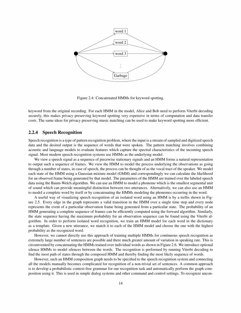
word 1

word 2

word 3

...

Garbage

Figure 2.4: Concatenated HMMs for keyword spotting.

keyword from the original recording. For each HMM in the model, Alice and Bob need to perform Viterbi decodingsecurely, this makes privacy preserving keyword spotting very expensive in terms of computation and data transfercosts. The same ideas for privacy preserving music matching can be used to make keyword spotting more efficient.

2.2.4 Speech Recognition

Speech recognition is a type of pattern recognition problem, where the input is a stream of sampled and digitized speechdata and the desired output is the sequence of words that were spoken. The pattern matching involves combiningacoustic and language models to evaluate features which capture the spectral characteristics of the incoming speechsignal. Most modern speech recognition systems use HMMs as the underlying model.

We view a speech signal as a sequence of piecewise stationary signals and an HMM forms a natural representationto output such a sequence of frames. We view the HMM to model the process underlying the observations as goingthrough a number of states, in case of speech, the process can be thought of as the vocal tract of the speaker. We modeleach state of the HMM using a Gaussian mixture model (GMM) and correspondingly we can calculate the likelihoodfor an observed frame being generated by that model. The parameters of the HMM are trained over the labeled speechdata using the Baum-Welch algorithm. We can use an HMM to model a phoneme which is the smallest segmental unitof sound which can provide meaningful distinction between two utterances. Alternatively, we can also use an HMMto model a complete word by itself or by concatenating the HMMs modeling the phonemes occurring in the word.

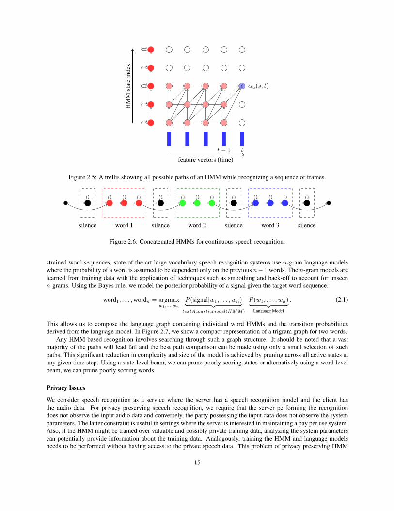
A useful way of visualizing speech recognition of an isolated word using an HMM is by a trellis shown in Fig-ure 2.5. Every edge in the graph represents a valid transition in the HMM over a single time step and every noderepresents the event of a particular observation frame being generated from a particular state. The probability of anHMM generating a complete sequence of frames can be efficiently computed using the forward algorithm. Similarly,the state sequence having the maximum probability for an observation sequence can be found using the Viterbi al-gorithm. In order to perform isolated word recognition, we train an HMM model for each word in the dictionaryas a template. Given a new utterance, we match it to each of the HMM model and choose the one with the highestprobability as the recognized word.

However, we cannot directly use this approach of training multiple HMMs for continuous speech recognition asextremely large number of sentences are possible and there much greater amount of variation in speaking rate. This iscircumvented by concatenating the HMMs trained over individual words as shown in Figure 2.6. We introduce optionalsilence HMMs to model silences between the words. The recognition is performed by running Viterbi decoding tofind the most path of states through the composed HMM and thereby finding the most likely sequence of words.

However, such an HMM composition graph needs to be specified to the speech recognition system and connectingall the models manually becomes complicated for recognition of a non-trivial set of sentences. A common approachis to develop a probabilistic context-free grammar for our recognition task and automatically perform the graph com-position using it. This is used in simple dialog systems and other command and control settings. To recognize uncon-

14

HM

Mst

ate

inde

x

feature vectors (time)

s αu(s, t)

t− 1 t

Figure 2.5: A trellis showing all possible paths of an HMM while recognizing a sequence of frames.

silence word 1 silence word 2 silence word 3 silence

Figure 2.6: Concatenated HMMs for continuous speech recognition.

strained word sequences, state of the art large vocabulary speech recognition systems use n-gram language modelswhere the probability of a word is assumed to be dependent only on the previous n− 1 words. The n-gram models arelearned from training data with the application of techniques such as smoothing and back-off to account for unseenn-grams. Using the Bayes rule, we model the posterior probability of a signal given the target word sequence.

word1, . . . ,wordn = argmaxw1,...,wn

P (signal|w1, . . . , wn)︸ ︷︷ ︸textAcousticmodel(HMM)

P (w1, . . . , wn)︸ ︷︷ ︸Language Model

. (2.1)

This allows us to compose the language graph containing individual word HMMs and the transition probabilitiesderived from the language model. In Figure 2.7, we show a compact representation of a trigram graph for two words.

Any HMM based recognition involves searching through such a graph structure. It should be noted that a vastmajority of the paths will lead fail and the best path comparison can be made using only a small selection of suchpaths. This significant reduction in complexity and size of the model is achieved by pruning across all active states atany given time step. Using a state-level beam, we can prune poorly scoring states or alternatively using a word-levelbeam, we can prune poorly scoring words.

Privacy Issues

We consider speech recognition as a service where the server has a speech recognition model and the client hasthe audio data. For privacy preserving speech recognition, we require that the server performing the recognitiondoes not observe the input audio data and conversely, the party possessing the input data does not observe the systemparameters. The latter constraint is useful in settings where the server is interested in maintaining a pay per use system.Also, if the HMM might be trained over valuable and possibly private training data, analyzing the system parameterscan potentially provide information about the training data. Analogously, training the HMM and language modelsneeds to be performed without having access to the private speech data. This problem of privacy preserving HMM

15

< s >

word 1

word 2

word 1

word 2

word 1

word 2

< /s >

P (word1| <s >

)

P (word2| <s >)

P (word

1| <s >

word1

)

P (word2| < s > word1)

P (word1| < s > word2)P (word2| <

s >word2)

P (word1|word1word1)

P(<s>|word1w

ord1)P

(word

2|word

2word

1)

P (word2|word2word2)

P(<s>|word2word2

)

Figure 2.7: Trigram language graph for recognizing < s >,word1, word2,< /s >.

inference falls under the area of secure multiparty computation (Section 3.1), and suitable protocols can be designedusing primitives such as homomorphic encryption. Isolated word recognition using a single HMM per word can beperformed using the forward algorithm. It is relatively straightforward to construct a practical privacy preservingsolution because of the linear complexity of the forward algorithm.

In continuous speech recognition by composite HMMs, the client and server need to collaborate in constructing atrellis structure indexed by the HMM states and the input sequences, and performing Viterbi decoding to identify theoptimal path. While we need to match one HMM per word in case of isolated word recognition, the client privatelyneeds to compare each frame of the input sequence to a graph of HMMs. This poses a number of problems owing tothe size of the search space and the sheer number of operations that need to be performed privately. Pruning involveseliminating search paths in the graph which are unlikely to be the best paths. By evaluating individual search paths,the server will gain a lot of information about what words are likely or unlikely to be in the search path using the inputdata belonging to the user. Hence, by its nature, pruning is contrary to the privacy constraints and we cannot makeadvantage of it to increase the speed and scalability of the recognition.

Given the state of the art of research, we believe that continuous speech recognition with privacy constraints iscurrently infeasible.

16

Chapter 3

Background on Privacy and Security

3.1 Secure Multiparty Computation

Secure Multiparty Computation (SMC) consists of the setting in which individual parties jointly compute a function oftheir private input data with the constraint that no party should learn anything apart from the output and the intermediatesteps of the computation. Informally, the security of an SMC protocol is defined as computational indistinguishabilityfrom an ideal functionality in which a trusted arbitrator accepts the input from all the parties, performs the computationand returns the results to all the parties. The actual protocol is secure if it does not leak any information beyond whatis leaked in the ideal functionality. Please refer to [Beaver, 1991; Canetti, 2000; Goldreich, 2004] for formal definitonsand theoretical models for analyzing SMC protocols.

Yao [1982] originally illustrated SMC using the millionaire problem where two parties are trying to identify whohas more money without disclosing the actual values of their amounts. In this seminal work, Yao also showed that anypolynomial-time multiparty computation can be performed with privacy in general but the generic techniques resultin computationally impractical solutions. Recent research has focused on constructing efficient privacy preservingprotocols for specific problems.

3.1.1 Data Setup and Privacy Conditions

We formally define the problem, in which multiple parties are interested in computing a function over their collectivelyheld datasets without disclosing any information to each other. For simplicity, we first consider the case of two parties,Alice and Bob. The parties are assumed to be semi-honest which means that the parties will follow the steps of theprotocol correctly and will not try to cheat by passing falsified data aimed at extracting information about other parties.The parties are assumed to be curious in the sense that they may record the outcomes of all intermediate steps of theprotocol to extract any possible information.

We assume that both the datasets can be represented as matrices in which columns and rows correspond to the datasamples and the features, respectively. For instance, the individual email collections of Alice and Bob are representedas matricesA andB respectively, in which the columns correspond to the emails, and the rows correspond to the words.The entries of these matrices represent the frequency of occurrence of a given word in a given email. The combineddataset may be split between Alice and Bob in two possible ways. In a horizontal split or data split, both Alice andBob have a disjoint set of data samples with the same features. The aggregate dataset is obtained by concatenatingcolumns given by the data matrix M =

[A B

]and correlation matrix MTM . In a vertical split or feature split,

Alice and Bob have different features of the same data. The aggregate data matrix M is obtained by concatenating

rows given by the data matrix M =

[AB

]and correlation matrix MMT .

17

3.1.2 Tools for Constructing SMC protocols1. Homomorphic Encryption. A homomorphic encryption (HE) cryptosystem allows for operations to be per-

form on the encrypted data without requiring to know the unencrypted values. If · and + are two operators andx and y are two plaintext elements, a homomorphic encryption function ξ() satisfies E[x] · E[y] = E[x+ y].

Owing to this property, simple operations can be performed directly on the ciphertext, thereby resulting insome desirable manipulations on the underlying plaintext messages. Additively homomorphic cryptosystemshave been proposed in the literature by Benaloh [1994], Paillier [1999] and Damgard and Jurik [2001]. Theprotocols that we construct in this paper can be executed with any of these cryptosystems. We primarily usethe asymmetric key Paillier cryptosystem [Paillier, 1999] which provides additive homomorphism as well assemantic security.

(a) Key Generation. Choose two large prime numbers p, q, and let N = pq. Denote by Z∗N2 ⊂ ZN2 ={0, 1, ..., N2 − 1} the set of non-negative integers that have multiplicative inverses modulo N2. Selectg ∈ Z∗N2 such that gcd(L(gλ mod N2), N) = 1, where λ = lcm(p − 1, q − 1), and L(x) = x−1

N . Let(N, g) be the public key, and (p, q) be the private key.

(b) Encryption. Let m ∈ ZN be a plaintext. Then, the ciphertext is given by

ξr(m) = gm · rN mod N2 (3.1)

where r ∈ Z∗N is a number chosen at random.

(c) Decryption. Let c ∈ ZN2 be a ciphertext. Then, the corresponding plaintext is given by

ψ(ξr(m)) =L(cλ mod N2)

L(gλ mod N2)= m mod N (3.2)

Note that decryption works irrespective of the value of r used during encryption. Since r can be chosen atrandom for every encryption, the Paillier cryptosystem is probabilistic, and therefore semantically secure. It cannow be verified that the following homomorphic properties hold for the mapping (3.1) from the plaintext set(ZN ,+) to the ciphertext set (Z∗N2 , ·),

ψ(ξr1(m1)ξr2(m2) mod N2) = m1 +m2 mod N

ψ( [ ξr(m1) ]m2 mod N2) = m1m2 mod N

where r1, r2 ∈ Z∗N and r1 6= r2 in general.

2. Oblivious Transfer.Oblivious transfer (OT) was originally introduced in Rabin [1981]. In an oblivious transfer protocol, the sendersends a collection of items to the receiver but remains oblivious about which item is valid.

Suppose that Bob has n messages m1,m2, . . .mn and Alice has the index 1 ≤ i ≤ n, oblivious transferensures that (a) Alice obtains mi but discovers nothing about the other messages (b) Bob does not discover i.There are many known ways to implement oblivious transfer such as those given by Naor and Pinkas [1999].Also, it has been shown that oblivious transfer is a sufficient primitive, i.e., it can be used for secure evaluationany function, provided that function can be represented as an algebraic circuit. However, evaluating generalfunctions using oblivious transfer exclusively is very expensive in terms of data transfer and computationalcosts; we use oblivious transfer sparingly in our protocols.

3. Blind and Permute. If the input c1, c2, . . . , cn is additively split among two parties with one party havinga1, a2, . . . , an and other party having b1, b2, . . . , bn, the parties can participate in a blind and permute proto-col [Atallah and Li, 2005] to obtain a randomly permuted additive split of the input such that the permutationis not known to either of the parties. This is useful in cases such as computing max ci securely. The blind andpermute primitive in turn uses homomorphic encryption and oblivious transfer.

18

3.1.3 Related Work on SMC Protocols for Machine Learning and Speech ProcessingThere has been a lot of work on constructing privacy preserving algorithms for specific problems in privacy preservingdata mining such as decision trees [Vaidya et al., 2008a], set matching [Freedman et al., 2004], clustering [Lin et al.,2005], association rule mining [Kantarcioglu and Clifton, 2004], naive Bayes classification [Vaidya et al., 2008b],support vector machines [Vaidya et al., 2008c]. Please refer to [Lindell and Pinkas, 2009] for a summary of recentwork.

However, there has been somewhat limited work on SMC protocols for speech processing applications, whichis one of the motivations for this thesis. Probabilistic inference with privacy constraints is a relatively unexploredarea of research. The only detailed treatment of privacy-preserving probabilistic classification appears in [Smaragdisand Shashanka, 2007]. In that work, inference via HMMs is performed on speech data using existing cryptographicprimitives. The protocols are based on repeated invocations of privacy-preserving two-party maximization algorithms,in which both parties incur exactly the same protocol overhead.

3.2 Differential PrivacyThe differential privacy model was originally introduced by Dwork [2006]. Given any two databases D and D′

differing by one element, which we will refer to as adjacent databases, a randomized query function M is said to bedifferentially private if the probability that M produces a response S on D is close to the probability that M producesthe same response S on D′. As the query output is almost the same in the presence or absence of an individualentry with high probability, nothing can be learned about any individual entry from the output. Differential privacy isformally defined as follows.

Definition. A randomized function M with a well-defined probability density P satisfies ε-differential privacy if, forall adjacent databases D and D′ and for any set of outcomes S ∈ range(M),∣∣∣∣log

P [M(D) ∈ S]

P [M(D′) ∈ S]

∣∣∣∣ ≤ ε. (3.3)

Dwork et al. [2006] proposed the exponential mechanism for creating functions satisfying ε-differential privacy byadding a perturbation term from the Laplace distribution scaled by the function sensitivity and ε, which is defined asthe maximum change in the value of the function when evaluated over adjacent datasets.

In a classification setting, the training dataset may be thought of as the database and the algorithm learning theclassification rule as the query mechanism. A classifier satisfying differential privacy implies that no additional detailsabout the individual training data instances can be obtained with certainty from output of the learning algorithm,beyond the a priori background knowledge. An adversary who observes the values for all except one entry in thedataset and has prior information about the last entry cannot learn anything with high certainty about the value of thelast entry beyond what was known a priori by observing the output of the mechanism over the dataset.

Differential privacy provides an ad omnia guarantee as opposed to most other models that provide ad hoc guar-antees against a specific set of attacks and adversarial behaviors. By evaluating the differentially private classifierover a large number of test instances, an adversary cannot learn the exact form of the training data. This is a strongerguarantee than SMC where the only condition is that the parties are not able to learn anything about the individualdata beyond what may be inferred from the final result of the computation. For instance, when the outcome of thecomputation is a classifier, it does not prevent an adversary from postulating the presence of data instances whoseabsence might change the decision boundary of the classifier, and verifying the hypothesis using auxiliary informationif any. Moreover, for all but the simplest computational problems, SMC protocols tend to be highly expensive, requir-ing iterated encryption and decryption and repeated communication of encrypted partial results between participatingparties.

3.2.1 Related Work on Differentially Private Machine LearningThe earlier work on differential privacy was related to functional approximations for simple data mining tasks anddata release mechanisms [Dinur and Nissim, 2003; Dwork and Nissim, 2004; Blum et al., 2005; Barak et al., 2007].

19

Although many of these works have connection to machine learning problems, more recently the design and analysisof machine learning algorithms satisfying differential privacy has been actively studied. Kasiviswanathan et al. [2008]present a framework for converting a general agnostic PAC learning algorithm to an algorithm that satisfies privacyconstraints. Chaudhuri and Monteleoni [2008] use the exponential mechanism [Dwork et al., 2006] to create a dif-ferentially private logistic regression classifier by adding Laplace noise to the estimated parameters. They proposeanother differentially private formulation which involves modifying the objective function of the logistic regressionclassifier by adding a linear term scaled by Laplace noise. The second formulation is advantageous because it is in-dependent of the classifier sensitivity which difficult to compute in general and it can be shown that using a perturbedobjective function introduces a lower error as compared to the exponential mechanism.

However, the above mentioned differentially private classification algorithms only address the problem of binaryclassification. Although it is possible to extend binary classification algorithms to multi-class using techniques likeone-vs-all, it is much more expensive to do so as compared to a naturally multi-class classification algorithm. Jagan-nathan et al. [2009] present a differentially private random decision tree learning algorithm which can be applied tomulti-class classification. Their approach involves perturbing leaf nodes using the sensitivity method, and they do notprovide theoretical analysis of excess risk of the perturbed classifier.

20

Chapter 4

Preliminary Work

We review the preliminary results of our research.

4.1 Techniques

4.1.1 Privacy Preserving Eigenvector ComputationWe developed a protocol for computing the principal eigenvector of the combined data shared by multiple partiescoordinated by a semi-honest arbitrator Trent [Pathak and Raj, 2010c]. This protocol is significantly more efficientthan the previous approaches towards this problem which are based on expensive QR decomposition of correlationmatrices. This was our first attempt at designing privacy preserving protocols. While it is not directly related to speechprocessing per se, many algorithms for probabilistic inference such as the forward backward algorithm for HMMsperform computation which is similar to eigenvector computation.

The power iteration algorithm computes the principal eigenvector of MTM by updating and normalizing thevector xt until convergence. Starting with a random vector x0, we calculate

xi+1 =MTM xi‖MTM xi‖

.

We first consider the case in which two parties Alice and Bob with horizontally split data matrices Ak×m and Bk×ncompute the principal eigenvector of the combined data in collaboration with an untrusted third party arbitrator Trent.For privacy, we split the vector xi into two parts, αi and βi. αi corresponds to the first m components of xi and βicorresponds to the remaining n components. In each iteration, we need to securely compute

MTMxi =

[ATA ATBBTA BTB

] [αiβi

]=

[AT (Aαi +Bβi)BT (Aαi +Bβi)

]=

[ATuiBTui

](4.1)

where ui = Aαi + Bβi. After convergence, αi and βi will represent shares held by Alice and Bob of the principaleigenvector of MTM .

An iteration of the algorithm proceeds as illustrated in Figure 4.1. At the outset Alice and Bob randomly generatecomponent vectors α0 and β0 respectively. At the beginning of the ith iteration, Alice and Bob possess componentvectors αi and βi respectively. They compute the product of their data and their corresponding component vectors asAαi andBβi. To compute ui, Alice and Bob individually transfer these products to Trent. Trent adds the contributionsfrom Alice and Bob by computing

ui = Aαi +Bβi.

He then transfers ui back to Alice and Bob, who then individually compute ATui and BTui, without requiring datafrom one other. For normalization, Alice and Bob also need to securely compute the term

‖MTM xi‖ =√‖ATui‖2 + ‖BTui‖2. (4.2)

21

Alice

Trent

Bob

E[Aαi +Bβi] = E[ui]

Aαi

E[Aαi]

Bβi

E[Bβi]

E[ui]

ATui

E[ui]

BTui

E[‖ATui‖2 + ‖BTui‖2]

‖ATui‖2

E[‖ATui‖2]

‖BTui‖2

E[‖BTui‖2]

αi+1 = ATui√‖ATui‖2+‖BTui‖2

βi+1 = BTui√‖ATui‖2+‖BTui‖2

Figure 4.1: Visual description of the protocol.

Again, Alice and Bob compute the individual terms ‖ATui‖2 and ‖BTui‖2 respectively and transfer it to Trent. Asearlier, Trent computes the sum

‖ATui‖2 + ‖BTui‖2

and transfers it back to Alice and Bob. Finally, Alice and Bob respectively update α and β vectors as

ui = Aαi +Bβi,

αi+1 =ATui√

‖ATui‖2 + ‖BTui‖2,

βi+1 =BTui√

‖ATui‖2 + ‖BTui‖2. (4.3)

The algorithm terminates when the α and β vectors converge.The basic protocol described above is provably correct. After convergence, Alice and Bob end up with the princi-

pal eigenvector of the row space of the combined data, as well as concatenative shares of the column space which Trentcan gather to compute the principal eigenvector. However the protocol is not completely secure; Alice and Bob ob-tain sufficient information about properties of each others’ data matrices, such as their column spaces, null spaces, andcorrelation matrices. We present a series of modifications to the basic protocol so that such information is not revealed.

Homomorphic Encryption: Securing the data from Trent

The central objective of the protocol is to prevent Trent from learning anything about either the individual data setsor the combined data other than the principal eigenvector of the combined data. Trent receives a series of partialresults of the form AATu, BBTu and MMTu. By analyzing these results, he can potentially determine the entirecolumn spaces of Alice and Bob as well as the combined data. To prevent this, we employ an additive homomorphiccryptosystem.

At the beginning of the protocol, Alice and Bob obtain a shared public key/private key pair for an additive homo-morphic cryptosystem from an authenticating authority. The public key is also known to Trent who, however, doesnot know the private key; While he can encrypt data, he cannot decrypt it. Alice and Bob encrypt all transmissionsto Trent, at the first transmission step of each iteration Trent receives the encrypted inputs E[Aαi] and E[Bβi]. Hemultiplies the two element by element to compute E[Aαi] · E[Bβi] = E[Aαi + Bβi] = E[ui]. He returns E[ui] toboth Alice and Bob who decrypt it with their private key to obtain ui. In the second transmission step of each iteration,Alice and Bob send E[‖ATui‖2] and E[‖BTui‖2] respectively to Trent, who computes the encrypted sum

E[‖ATui‖2

]· E[‖BTui‖2

]= E

[‖ATui‖2 + ‖BTui‖2

]22

and transfers it back to Alice and Bob, who then decrypt it to obtain ‖ATui‖2 + ‖BTui‖2, which is required fornormalization.

This modification does not change the actual computation of the power iterations in any manner. Thus the proce-dure remains as correct as before, except that Trent now no longer has any access to any of the intermediate compu-tations. At the termination of the algorithm he can now receive the converged values of α and β from Alice and Bob,who will send it in clear text.

Random Scaling: Securing the Column Spaces

After Alice and Bob receive ui = Aαi +Bβi from Trent, Alice can calculate ui −Aαi = Bβi and Bob can calculateui −Bβi = Aαi. After a sufficient number of iterations, particularly in the early stages of the computation (when uihas not yet converged) Alice can find the column space of B and Bob can find the column space of A. Similarly, bysubtracting their share from the normalization term returned by Trent, Alice and Bob are able to find ‖BTui‖2 and‖ATui‖2 respectively.

In order to prevent this, Trent multiplies ui with a randomly generated scaling term ri that he does not share withanyone. Trent computes

(E[Aαi] · E[Bβi])ri = E[ri(Aαi +Bβi)] = E[riui]

by performing element-wise exponentiation of the encrypted vector by ri and transfers riui to Alice and Bob. Byusing a different value of ri at each iteration, Trent ensures that Alice and Bob are not able to calculate Bβi and Aαirespectively. In the second step, Trent scales the normalization constant by r2

i ,(E[‖ATui‖2

]· E[‖BTui‖2

])r2i = E[r2i

(‖ATi u‖2 + ‖BTi u‖2

)].

Normalization causes the ri factor to cancel out and the update rules remain unchanged.

ui = Aαi +Bβi,

αi+1 =riA

Tui√r2i (‖ATui‖2 + ‖BTui‖2)

=ATui√

‖ATui‖2 + ‖BTui‖2,

βi+1 =riB

Tui√r2i (‖ATui‖2 + ‖BTui‖2)

=BTui√

‖ATui‖2 + ‖BTui‖2. (4.4)

The random scaling does not affect the final outcome of the computation, and the algorithm remains correct as before.

Data Padding: Securing null spaces

In each iteration, Alice observes one vector riui = ri(Aαi + Bβi) in the column space of M = [A B]. Alice cancalculate the null space H(A) of A, given by

H(A) = {x ∈ Rm|Ax = 0}

and pre-multiply a non-zero vector x ∈ H(A) with riui to calculate

xriui = rix(Aαi +Bβi) = rixBβi.

This is a projection of Bβi, a vector in the column space of B into the null space H(A). Similarly, Bob can findprojections of Aαi in the null space H(B). While considering the projected vectors separately will not give awaymuch information, after several iterations Alice will have a projection of the column space of B on the null space ofA, thereby learning about the component’s of Bob’s data that lie in her null space. Bob can similarly learn about thecomponent’s of Alice’s data that lie in his null space.

In order to prevent this, Alice pads her data matrix A by concatenating it with a random matrix Pa = raIk×k, toobtain

[A Pa

]where ra is a positive scalar chosen by Alice. Similarly, Bob pads his data matrixB with Pb = rbIk×k

23

to obtain[B Pb

]where rb is a different positive scalar chosen by Bob. This has the effect of hiding the null spaces

in both their data sets. In the following theorem, we prove that the eigenvectors of the combined data do not changeafter padding, while every eigenvalue λ of MMT is now modified to λ + ra + rb. Please refer to appendix for theproof.

Theorem 4.1.1. Let M =[M P

]where M is a s× t matrix, and P is a s× s orthogonal matrix. If v =

[vt×1

v′s×1

]is

an eigenvector of MT M corresponding to an eigenvalue λ, then v is an eigenvector of MTM .

While the random factors ra and rb prevent Alice and Bob from estimating the eigenvalues of the data, the com-putation of principal eigenvector remains correct as before.

Oblivious Transfer: Securing Krylov spaces

For a constant c, we can show that the vector ui = Aαi + Bβi is equal to cMMTui−1. The sequence of vectorsU = {u1, u2, u3, . . .} form the Krylov subspace (MMT )nu1 of the matrix MMT . Knowledge of this series ofvectors can reveal all eigenvectors of MMT . Consider u0 = c1v1 + c2v2 + · · · , where vi is the ith eigenvector. If λjis the jth eigenvalue, we have ui = c1λ1v1 +c2λ2v2 + · · · . We assume wlog that the eigenvalues λ are in a descendingorder, i.e., λj ≥ λk for j < k. Let uconv be the normalized converged value of ui which is equal to the normalizedprincipal eigenvector v1.

Let wi = ui − (ui · uconv)ui which can be shown to be equal to c2λ2v2 + c3λ3v3 + · · · , i.e., a vector with nocomponent along v1. If we perform power iterations with initial vector w1, the converged vector wconv will be equalto the eigenvector corresponding to the second largest eigenvalue. Hence, once Alice has the converged value, uconv ,she can subtract it out of all the stored ui values and determine the second principal eigenvector of MMT . She canrepeat the process iteratively to obtain all eigenvectors ofMMT , although in practice the estimates become noisy veryquickly. The following modification prevents Alice and Bob from identifying the Krylov space with any certainty andthey are thereby unable to compute the additional eigenvectors of the combined data.

We introduce a form of oblivious transfer (OT) [Rabin, 1981] in the protocol. We assume that Trent stores theencrypted results of intermediate steps at every iteration. After computing E[riui], Trent either sends this quantity toAlice and Bob with a probability p or sends a random vector E[u′i] of the same size (k × 1) with probability 1 − p.As the encryption key of the cryptosystem is publicly known, Trent can encrypt the vector u′i. Alice and Bob do notknow whether they are receiving riui or u′i. If a random vector is sent, Trent continues with the protocol, but ignoresthe terms Alice and Bob return in the next iteration, E[Aαi+1] and E[Bβi+1]. Instead, he sends the result of a the lastnon-random iteration j, E[rjuj ], thereby restarting that iteration.

This sequence of data sent by Trent is an example of a Bernoulli Process [Papoulis, 1984]. An illustrative exampleof the protocol is shown in Figure 4.2. In the first two iterations, Trent sends valid vectors r1u1 and r2u2 back to Aliceand Bob. In the beginning of the third iteration, Trent receives and computes E[r3u3] but sends a random vector u′3.He ignores what Alice and Bob send him in the fourth iteration and sends back E[r3u3] instead. Trent then stores thevector E[r4u4] sent by Alice and Bob in the fifth iteration and sends a random vector u′2. Similarly, he ignores thecomputed vector of the sixth iteration and sends u′3. Finally, he ignores the computed vector of the seventh iterationand sends E[r4u4].

r1u1 r2u2 u′1 r3u3 u′2 u′3 r4u4

Figure 4.2: An example of the protocol execution with oblivious transfer.

This modification has two effects – firstly it prevents Alice and Bob from identifying the Krylov space withcertainty. As a result, they are now unable to obtain additional Eigenvectors from the data. Secondly, oblivious transfer

24

essentially obfuscates the projection of the column space of B on to the null space of A for Alice, and analogously forBob by introducing random vectors. As Alice and Bob do not know which vectors are random, they cannot completelycalculate the true projection of each others data on the null spaces. This is rendered less important if Alice and Bobpad their data as suggested in the previous subsection.

Alice and Bob can store the vectors they receive from Trent in each iteration. By analyzing the distribution ofthe normalized vectors, Alice and Bob can identify the random vectors using a simple outlier detection technique. Toprevent this, one possible solution is for Trent to pick a previously computed value of rjuj and add zero mean noiseei, for instance, sampled from the Gaussian distribution.

u′i = rjuj + ei, ei ∼ N (0, σ2).

Instead of transmitting a perturbation of a previous vector, Trent can also use perturbed mean of a few previous rjujwith noise. Doing this will create a random vector with the same distributional properties as the real vectors. Thenoise variance parameter σ controls the error in identifying the random vector from the valid vectors and how mucherror do we want to introduce in the projected column space.

Oblivious transfer has the effect of increasing the total computation as every iteration in which Trent sends a ran-dom vector is wasted. In any secure multi-party computation, there is an inherent trade-off between computation timeand the degree of security. The parameter p which is the probability of Trent sending a non-random vector allows usto control this at a fine level based on the application requirements. As before, introducing oblivious transfer does notaffect the correctness of the computation – it does not modify the values of the non-random vectors ui.

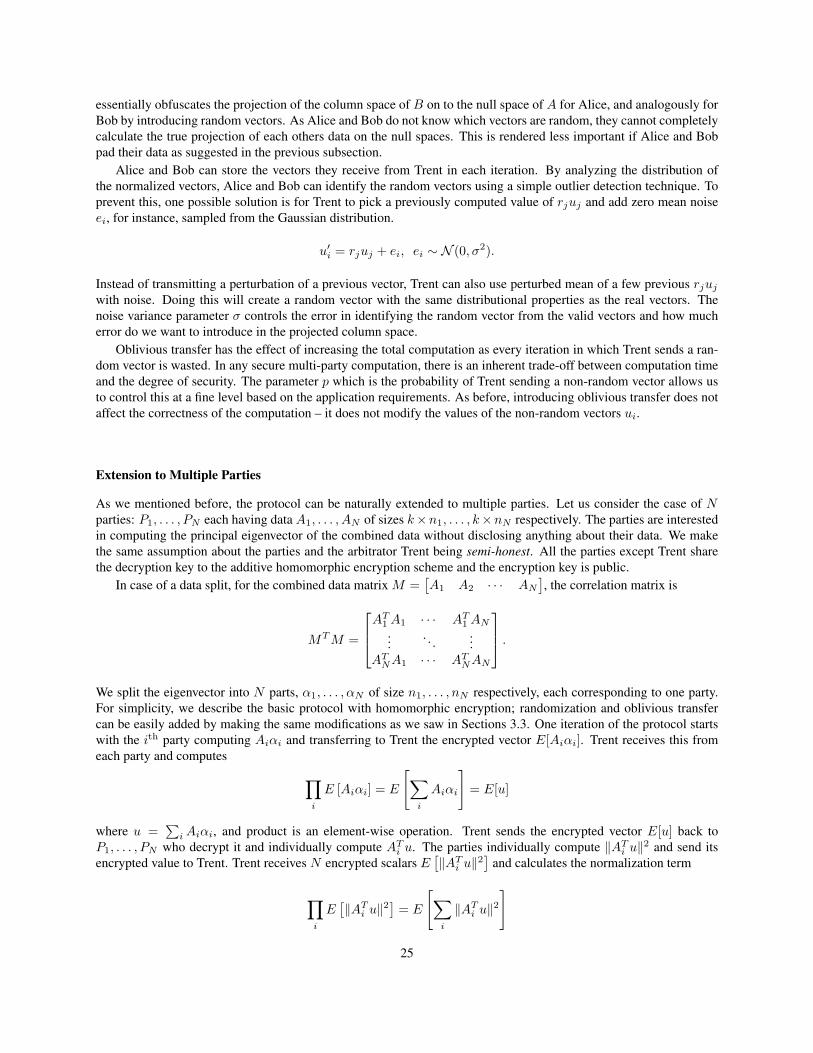
Extension to Multiple Parties

As we mentioned before, the protocol can be naturally extended to multiple parties. Let us consider the case of Nparties: P1, . . . , PN each having data A1, . . . , AN of sizes k×n1, . . . , k×nN respectively. The parties are interestedin computing the principal eigenvector of the combined data without disclosing anything about their data. We makethe same assumption about the parties and the arbitrator Trent being semi-honest. All the parties except Trent sharethe decryption key to the additive homomorphic encryption scheme and the encryption key is public.

In case of a data split, for the combined data matrix M =[A1 A2 · · · AN

], the correlation matrix is

MTM =

AT1 A1 · · · AT1 AN...

. . ....

ATNA1 · · · ATNAN

.We split the eigenvector into N parts, α1, . . . , αN of size n1, . . . , nN respectively, each corresponding to one party.For simplicity, we describe the basic protocol with homomorphic encryption; randomization and oblivious transfercan be easily added by making the same modifications as we saw in Sections 3.3. One iteration of the protocol startswith the ith party computing Aiαi and transferring to Trent the encrypted vector E[Aiαi]. Trent receives this fromeach party and computes ∏

i

E [Aiαi] = E

[∑i

Aiαi

]= E[u]

where u =∑iAiαi, and product is an element-wise operation. Trent sends the encrypted vector E[u] back to

P1, . . . , PN who decrypt it and individually compute ATi u. The parties individually compute ‖ATi u‖2 and send itsencrypted value to Trent. Trent receives N encrypted scalars E

[‖ATi u‖2

]and calculates the normalization term

∏i

E[‖ATi u‖2

]= E

[∑i

‖ATi u‖2]

25

and sends it back to the parties. At the end of the iteration, the party Pi updates αi as

u =∑i

Aiα(old)i ,

α(new)i =

ATi u√∑i ‖ATi u‖2

. (4.5)

The algorithm terminates when any one party Pi converges on αi.

4.1.2 Differentially Private Large Margin Gaussian Mixture Models

We developed a learning algorithm for discriminatively trained Gaussian mixture models which satisfies differentialprivacy [Pathak and Raj, 2010a,b] and is the first multiclass classification algorithm doing so.

Large Margin Gaussian Classifiers

There has been work on learning GMM while satisfying the large margin property [Sha and Saul, 2006]. This leads tothe classification algorithm being robust to outliers with provably strong generalization guarantees.

We first consider the setting where each class is modeled as a single Gaussian ellipsoid. Each class is modeled bya set of K Gaussian ellipsoids. The decision rule is to assign an instance ~xi to the class having smallest Mahalanobisdistance [Mahalanobis, 1936] from ~xi to the centroid of that class. We apply the large margin intuition about the clas-sifier maximizing the distance of training data instances from the decision boundaries having a lower error. Formally,we require that for each training data instance ~xi with label yi, the distance from ~xi to the centroid of class yi is atleast less than its distance from centroids of all other classes by one.

∀c 6= yi : ~xTi Φc~xi ≥ 1 + ~xTi Φyi~xi. (4.6)

Analogous to support vector machines, the training algorithm is an optimization problem minimizing the hinge lossdenoted by [f ]+ = max(0, f), with a linear penalty for incorrect classification. We use the sum of traces of inversecovariance matrices for each classes as a regularization term.

J(Φ, ~x, ~y) =∑i

∑c6=yi

[1 + ~xTi (Φyi −Φc)~xi

]+

+ λ∑c

trace(Ψc). (4.7)

Generalizing to Mixtures of Gaussians

We extend the above classification framework to modeling each class as a mixture ofK Gaussians ellipsoids. A simpleextension is to consider each data instance ~xi as having a mixture component mi along with the label yi. The mixturelabels are not available a priori, these can be generated by training a generative GMM using the data instances in eachclass and selecting the mixture component with the highest posterior probability. Similar to the single Gaussian perclass criterion, we require that for each training data instance ~xi with label yi and mixture component mi, the distancefrom ~xi to the centroid of the Gaussian ellipsoid for the mixture component mi of label yi is at least one greater thanthe minimum distance from ~xi to the centroid of any mixture component of any other class.

∀c 6= yi : minm

~xTi Φcm~xi ≥ 1 + ~xTi Φyi,mi~xi.

In order to maintain the convexity of the objective function, we use the property minm am ≥ − log∑m e−am to

rewrite the above constraint as

∀c 6= yi : − log∑m

e−~xTi Φcm~xi ≥ 1 + ~xTi Φyi,mi~xi. (4.8)

26

1 − h

1 + h

Figure 4.3: Hinge loss

As before, we minimize the hinge loss of misclassification along with the regularization term. The objective functionbecomes

J(Φ, ~x, ~y) =∑i

∑c6=yi

[1 + ~xTi Φyi~xi + log

∑m

e−~xTi Φc~xi

]+

+ λ∑cm

trace(IΦΦcmIΦ). (4.9)

It can be observed that after this modification, the optimization problem remains a convex semidefinite program andis tractable to solve.

Making the Objective Function Differentiable

The hinge loss being non-differentiable is not convenient for our analysis; we replace it with a surrogate loss functioncalled Huber loss lh [Chapelle, 2007] which has similar characteristics as the hinge loss for small values of h. Let usdenote ~xTi Φyi~xi+log

∑m e−~xTi Φc~xi by M(xi,Φc) for conciseness. The Huber loss `h computed over data instances

(~xi, yi) becomes

`h(Φc, ~xi, yi) =

0 if M(xi,Φc) > h,

14h

[h− ~xTi Φyi~xi − log

∑m e−~xTi Φc~xi

]2if |M(xi,Φc)| ≤ h

−~xTi Φyi~xi − log∑m e−~xTi Φc~xi if M(xi,Φc) < −h.

(4.10)

Finally, the regularized Huber loss computed over the the training dataset (x, ~y) is given by

J(Φ, ~x, ~y) =∑i

∑c6=yi

`h

[1 + ~xTi Φyi~xi + log

∑m

e−~xTi Φc~xi

]+ λ

∑cm

trace(IΦΦcmIΦ)

= L(Φ, ~x, ~y) +N(Φ), (4.11)

where L(Φ, ~x, ~y) is the loss function and N(Φ) is the regularization term.

Differentially Private Formulation

We modify the large margin Gaussian mixture model formulation to satisfy differential privacy by introducing aperturbation term in the objective function. We generate the size (d+ 1)× (d+ 1) perturbation matrix b with density

P (b) ∝ exp(− ε

2‖b‖

), (4.12)

where ‖ · ‖ is the Frobenius norm (element-wise `2 norm) and ε is the privacy parameter. One method of generatingsuch a b matrix is to sample the norm ‖b‖ from Γ

((d+ 1)2, 2

ε

)and the direction of b at random.

27

Our proposed learning algorithm minimizes the following objective function Jp(Φ, ~x, ~y)

Jp(Φ, ~x, ~y) = L(Φ, ~x, ~y) +N(Φ) +∑c

∑ij

bijΦcij . (4.13)

As the dimensionality of the perturbation matrix b is same as that of the classifier parameters Φc, the parameter spaceof Φ does not change after perturbation. In other words, given two datasets (~x, ~y) and (~x′, ~y′), if Φp minimizesJp(Φ, ~x, ~y), it is always possible to have Φp minimize Jp(Φ, ~x′, ~y′). This is a necessary condition for the classifierΦp satisfying differential privacy.

As the perturbation term is convex and positive semidefinite, the perturbed objective function Jp(Φ, ~x, ~y) has thesame properties as the unperturbed objective function J(Φ, ~x, ~y).

Proof of Differential Privacy

We prove that the classifier minimizing the perturbed optimization function Jp(Φ, ~x, ~y) satisfies ε-differential privacyin the following theorem. Given a dataset (~x, ~y) = {(~x1, y1), . . . , (~xn−1, yn−1), (~xn, yn)}, the probability of learningthe classifier Φp is close to the the probability of learning the same classifier Φp given an adjacent dataset (~x′, ~y′) ={(~x1, y1), . . . , (~xn−1, yn−1), (~x′n, y

′n)} differing wlog on the nth instance. As we mentioned in the previous section,

it is always possible to find such a classifier Φp minimizing both Jp(Φ, ~x, ~y) and Jp(Φ, ~x′, ~y′) due to the perturbationmatrix being in the same space as the optimization parameters.

Our proof requires a strictly convex perturbed objective function resulting in a unique solution Φp minimizing it.This in turn requires that the loss function L(Φ, ~x, y) is strictly convex and differentiable, and the regularization termN(Φ) is convex. These seemingly strong constraints are satisfied by many commonly used classification algorithmssuch as logistic regression, support vector machines, and our general perturbation technique can be extended to thosealgorithms. In our proposed algorithm, the Huber loss is by definition a differentiable function and the trace regular-ization term is convex and differentiable. Additionally, we require that the difference in the gradients of L(Φ, ~x, y)calculated over for two adjacent training datasets is bounded. We prove this property in Lemma A.2.1.

Theorem 4.1.2. For any two adjacent training datasets (~x, ~y) and (~x′, ~y′), the classifier Φp minimizing the perturbedobjective function Jp(Φ, ~x, ~y) satisfies differential privacy.∣∣∣∣log

P (Φp|~x, ~y)

P (Φp|~x′, ~y′)

∣∣∣∣ ≤ ε′,where ε′ = ε+ k for a constant factor k = log

(1 + 2α

nλ + α2

n2λ2

)with a constant value of α.

Analysis of Excess Risk

The perturbation introduced in the objective function comes at a cost of accuracy; when applied to any training dataset,the differentially private classifier will have an extra error as compared to the original classifier. We establish a boundon this excess risk.

In the remainder of this section, we denote the terms J(Φ,x,y) and L(Φ,x,y) by J(Φ) and L(Φ), respectivelyfor conciseness. The objective function J(Φ) contains the loss function L(Φ) computed over the training data (x,y)and the regularization term N(Φ) – this is known as the regularized empirical risk of the classifier Φ. In the followingtheorem, we establish a bound on the regularized empirical excess risk of the differentially private classifier minimizingthe perturbed objective function Jp(Φ) over the classifier minimizing the unperturbed objective function J(Φ). Weuse the strong convexity of the objective function J(Φ) as given by Lemma A.2.2.

Theorem 4.1.3. With probability at least 1 − δ, the regularized empirical excess risk of the classifier Φp minimizingthe perturbed objective function Jp(Φ) over the classifier Φ∗ minimizing the unperturbed objective function J(Φ) isbounded as

J(Φp) ≤ J(Φ∗) +8(d+ 1)4C

ε2λlog2

(d

δ

).

28

The upper bound on the regularized empirical risk is in O(Cε2 ). The bound increases for smaller values of ε whichimplies tighter privacy and therefore suggests a trade off between privacy and utility.

The regularized empirical risk of a classifier is calculated over a given training dataset. In practice, we are moreinterested in how the classifier will perform on new test data which is assumed to be generated from the samesource as the training data. The expected value of the loss function computed over the data is called the true riskL(Φ) = E[L(Φ)] of the classifier Φ. In the following theorem, we establish a bound on the true excess risk of thedifferentially private classifier minimizing the perturbed objective function and the classifier minimizing the originalobjective function.

Theorem 4.1.4. With probability at least 1 − δ, the true excess risk of the classifier Φp minimizing the perturbedobjective function Jp(Φ) over the classifier Φ∗ minimizing the unperturbed objective function J(Φ) is bounded as

L(Φp) ≤ L(Φ∗) +4√d(d+ 1)2C

ελlog

(d

δ

)+

8(d+ 1)4C

ε2λlog2

(d

δ

)+

16

λn

[32 + log

(1

δ

)].

Similar to the bound on the regularized empirical excess risk, the bound on the true excess risk is also inverselyproportional to ε reflecting the privacy-utility trade-off. The bound is linear in the number of classes C, which is aconsequence of the multi-class classification. The classifier learned using a higher value of the regularization parameterλ will have a higher covariance for each class ellipsoid. This would also make the classifier less sensitive to theperturbation. This intuition is confirmed by the fact that the true excess risk bound is inversely proportional to λ.

Experiments

We performed experiments with our differentially private large margin Gaussian classifier to observe how much erroris introduced by the perturbation. We implemented the classifier using the CVX convex program solver [Grant andBoyd, 2008, 2010] .

We trained the classifier with the different random samples of the perturbation term b, each sampled with theincreasing values of ε, and the regularization parameter λ = 0.01. For training data we used 500 data points with10 dimensions equally split into the five classes each randomly sampled from the Gaussian distributions with unitvariances. We tested the model on another 500 data points with 10 dimensions equally split into the five classes eachalso sampled from Gaussian distribution. The test error results averaged over 100 runs are shown in Figure 4.4.

Figure 4.4: Test error vs. ε

We observe that for small value of ε implying tighter privacy constraints, we observe a higher error. By increasingε, we see that the error steadily goes down as predicted by the bound on the true excess risk.

29

4.1.3 Differentially Private Classification from Multiparty DataIn [Pathak et al., 2010a], we address the problem of learning a differentially private classifier from a set of partieseach possess data. The aim is to learn a classifier from the union of all the data. We specifically consider a logisticregression classifier, but as we shall see, the techniques are generally applicable to any classification algorithm. Theconditions we impose are that (a) None of the parties are willing to share the data with one another or with any thirdparty (e.g. a curator). (b) The computed classifier cannot be reverse engineered to learn about any individual datainstance possessed by any contributing party.

We provide an alternative solution: within our approach the individual parties locally compute an optimal classifierwith their data. The individual classifiers are then averaged to obtain the final aggregate classifier. The aggregationis performed through a secure protocol that also adds a stochastic component to the averaged classifier, such that theresulting aggregate classifier is differentially private, i.e., no inference may be made about individual data instancesfrom the classifier. This procedure satisfies both criteria (a) and (b) mentioned above. Furthermore, it is significantlyless expensive than any SMC protocol to compute the classifier on the combined data.

Multiparty Classification Protocol

The problem we address is as follows: a number of parties P1, . . . , PK possess data sets D1, . . . , DK where Di =(x, y)|j includes a set of instances x and their binary labels y. We want to train a logistic regression classifier on thecombined data such that no party is required to expose any of its data, and the no information about any single datainstance can be obtained from the learned classifier. The protocol can be divided into the three following phases:

• Training Local Classifiers on Individual Datasets.Each party Pj uses their data set (x, y)|j to learn an `2 regularized logistic regression classifier with weights wj .This is obtained by minimizing the following objective function

wj = argminw

J(w) = argminw

1

nj

∑i

log(

1 + e−yiwT xi)

+ λwTw, (4.14)

where λ > 0 is the regularization parameter. Note that no data or information has been shared yet.

• Publishing a Differentially Private Aggregate Classifier. The proposed solution, illustrated by Figure 4.5, pro-ceeds as follows. The parties then collaborate to compute an aggregate classifier given by ws = 1

K

∑j wj + η,

where η is a d-dimensional random variable sampled from a Laplace distribution scaled with the parameter2

n(1)ελand n(1) = minj nj . As we shall see later, composing an aggregate classifier in this manner incurs only

a well-bounded excess risk over training a classifier directly on the union of all data while enabling the partiesto maintain their privacy. We also show that the noise term η ensures that the classifier ws satisfies differentialprivacy, i.e., that individual data instances cannot be discerned from the aggregate classifier. The definition ofthe noise term η above may appear unusual at this stage, but it has an intuitive explanation: A classifier con-structed by aggregating locally trained classifiers is limited by the performance of the individual classifier thathas the least number of data instances. We note that the parties Pj cannot simply take their individually trainedclassifiers wj , perturb them with a noise vector and publish the perturbed classifiers, because aggregating suchclassifiers will not give the correct η ∼ Lap

(2/(n(1)ελ)

)in general. Since individual parties cannot simply add

noise to their classifiers to impose differential privacy, the actual averaging operation must be performed suchthat the individual parties do not expose their own classifiers or the number of data instances they possess. Wetherefore use a private multiparty protocol, interacting with an untrusted curator “Charlie” to perform the aver-aging. The outcome of the protocol is such that each of the parties obtain additive shares of the final classifierws, such that these shares must be added to obtain ws.

Privacy Preserving Protocol. We use asymmetric key additively homomorphic encryption [Paillier, 1999]. Adesirable property of such schemes is that we can perform operations on the ciphertext elements which mapinto known operations on the same plaintext elements. For an additively homomorphic encryption function ξ(·),

30

curator

additive secret sharing

&

blind-and-permute

Indicator vector with permuted index of smallest database

curator

encryption

&

reverse permutations

&

add noise vectors

Encrypted Laplacian noise vectoradded obliviously by smallest database

curator

additive secret

sharing of noise term

&

additive secret

sharing of local

classifers

perfectly privateadditive shares of

Null

Stage 1 Stage 2 Stage 3

Figure 4.5: Multiparty protocol to securely compute additive shares of ws.

ξ(a) ξ(b) = ξ(a + b), ξ(a)b = ξ(ab). The additively homomorphic scheme employed here is semanticallysecure, i.e., repeated encryption of the same plaintext will result in different ciphertexts. For the ensuing pro-tocol, encryption keys are considered public and decryption keys are privately owned by the specified parties.Assuming the parties to be honest-but-curious, the steps of the protocol are as follows.

Stage 1. Finding the index of the smallest database obfuscated by permutation.

1. Each party Pj computes nj = aj + bj , where aj and bj are integers representing additive shares ofthe database lengths nj for j = 1, 2, . . . ,K. Denote the K-length vectors of additive shares as a andb respectively.

2. The partiesPj mutually agree on a permutation π1 on the index vector (1, 2, . . . ,K). This permutationis unknown to Charlie. Then, each party Pj sends its share aj to party Pπ1(j), and sends its share bjto Charlie with the index changed according to the permutation. Thus, after this step, the parties havepermuted additive shares given by π1(a) while Charlie has permuted additive shares π1(b).

3. The parties Pj generate a key pair (pk,sk) where pk is a public key for homomorphic encryption andsk is the secret decryption key known only to the parties but not to Charlie. Denote element-wiseencryption of a by ξ(a). The parties send ξ(π1(a)) = π1(ξ(a)) to Charlie.

4. Charlie generates a random vector r = (r1, r2, · · · , rK) where the elements ri are integers chosen uni-formly at random and are equally likely to be positive or negative. Then, he computes ξ(π1(aj))ξ(rj)= ξ(π1(aj) + rj). In vector notation, he computes ξ(π1(a) + r). Similarly, by subtracting the samerandom integers in the same order to his own shares, he obtains π1(b)− r where π1 was the permuta-tion unknown to him and applied by the parties. Then, Charlie selects a permutation π2 at random andobtains π2(ξ(π1(a) + r)) = ξ(π2(π1(a) + r)) and π2(π1(b)− r). He sends ξ(π2(π1(a) + r)) to theindividual parties in the following order: First element to P1, second element to P2,. . . ,K th elementto PK .

5. Each party decrypts the signal received from Charlie. At this point, the parties P1, P2, . . . , PKrespectively possess the elements of the vector π2(π1(a) + r) while Charlie possesses the vectorπ2(π1(b) − r). Since π1 is unknown to Charlie and π2 is unknown to the parties, the indices in bothvectors have been complete obfuscated. Note also that, adding the vector collectively owned by theparties and the vector owned by Charlie would give π2(π1(a)+r)+π2(π1(b)−r) = π2(π1(a+b)) =π2(π1(n)). This situation in this step is similar to that encountered in the “blind and permute” protocolused for minimum-finding by Atallah and Li [2005].

31

6. Let π2(π1(a)+r) = a and π2(π1(b)−r) = b. Then ni > nj ⇒ ai+bi > aj+bj ⇒ ai−aj > bj−bi.For each (i, j) pair with i, j ∈ {1, 2, . . . ,K}, these comparisons can be solved by any implementationof a secure millionaire protocol [Yao, 1982]. When all the comparisons are done, Charlie finds theindex j such that aj + bj = minj nj . The true index corresponding to the smallest database hasalready been obfuscated by the steps of the protocol. Charlie holds only an additive share of minj njand thus cannot know the true length of the smallest database.

Stage 2. Obliviously obtaining encrypted noise vector from the smallest database.

1. Charlie constructs an K indicator vector u such that uj = 1 and all other elements are 0. He thenobtains the permuted vector π−1

2 (u) where π−12 inverts π2. He generates a key-pair (pk′,sk′) for

additive homomorphic function ζ(·) where only the encryption key pk′ is publicly available to theparties Pj . Charlie then transmits ζ(π−1

2 (u)) = π−12 (ζ(u)) to the parties Pj .

2. The parties mutually obtain a permuted vector π−11 (π−1

2 (ζ(u))) = ζ(v) where π−11 inverts the per-

mutation π1 originally applied by the parties Pj in Stage I. Now that both permutations have beenremoved, the index of the non-zero element in the indicator vector v corresponds to the true indexof the smallest database. However, since the parties Pj cannot decrypt ζ(·), they cannot find out thisindex.

3. For j = 1, . . . ,K, party Pj generates ηj , a d-dimensional noise vector sampled from a Laplacedistribution with parameter 2

njελ. Then, it obtains a d-dimensional vector ψj where for i = 1, . . . , d,

ψj(i) = ζ(v(j))ηj(i) = ζ(v(j) ηj(i)).4. All parties Pj now compute a d-dimensional noise vector ψ such that, for i = 1, . . . , d, ψ(i) =∏

j ψj(i) =∏j ζ(v(j)ηj(i)) = ζ

(∑j v(j)ηj(i)

).

The reader will notice that, by construction, the above equation selects only the Laplace noise termsfor the smallest database, while rejecting the noise terms for all other databases. This is because v hasan element with value 1 at the index corresponding to the smallest database and has zeroes everywhereelse. Thus, the decryption of ψ is equal to η which was the desired perturbation term defined at thebeginning of this section.

Stage 3. Generating secret additive shares of ws.

1. One of the parties, say P1, generates a d-dimensional random integer noise vector s, and transmitsψ(i)ζ(s(i)) for all i = 1, . . . , d to Charlie. Using s effectively prevents Charlie from discovering η,and therefore still ensures that no information is leaked about the database owners Pj . P1 computesw1 −Ks.

2. Charlie decrypts ψ(i)ζ(s(i)) to obtain η(i) + s(i) for i = 1, . . . , d. At this stage, the parties andCharlie have the following d-dimensional vectors: Charlie has K(η + s), P1 has w1 − Ks, and allother parties Pj , j = 2, . . . ,K have wj . None of the K + 1 participants can share this data for fearof compromising differential privacy.

3. Finally, Charlie and the K database-owning parties run a simple secure function evaluation protocol[Ben-Or et al., 1988], at the end of which each of the K + 1 participants obtains an additive shareof Kws. This protocol is provably private against honest but curious participants when there are nocollisions. The resulting shares are published.

The above protocol ensures the following (a) None of the K + 1 participants, or users of the perturbed aggre-gate classifier can find out the size of any database, and therefore none of the parties knows who contributed η(b) Neither Charlie nor any of the parties Pj can individually remove the noise η after the additive shares arepublished. This last property is important because if anyone knowingly could remove the noise term, then theresulting classifier no longer provides differential privacy.

• Testing Phase. A test participant Dave having a test data instance x′ ∈ Rd is interested in applying the trainedclassifier adds the published shares and divides by K to get the differentially private classifier ws. He can then

32

compute the sigmoid function t = 1

1+e−wsT xiand decide to classify x′ with label −1 if t ≤ 1

2 and with label 1 if

t > 12 .

Proof of Differential Privacy

We show that the perturbed aggregate classifier satisfies differential privacy. We use the following bound on the sen-sitivity of the regularized regression classifier as proved in Corollary 2 in [Chaudhuri and Monteleoni, 2008] restatedin the appendix as Theorem A.3.1.

Theorem 4.1.5. The classifier ws preserves ε-differential privacy. For any two adjacent datasets D and D′,∣∣∣∣logP (ws|D)

P (ws|D′)

∣∣∣∣ ≤ ε.Analysis of Excess Risk

In the following discussion, we consider how much excess error is introduced when using a perturbed aggregateclassifier ws satisfying differential privacy as opposed to the unperturbed classifier w∗ trained on the entire trainingdata while ignoring the privacy constraints as well as the unperturbed aggregate classifier w.

We first establish a bound on the `2 norm of the difference between the aggregate classifier w and the classifier w∗trained over the entire training data. To prove the bound we apply Lemma 1 from [Chaudhuri and Monteleoni, 2008]restated as Lemma A.3.2 in the appendix. Please refer to the appendix for the proof of the following theorem.

Theorem 4.1.6. Given the aggregate classifier w, the classifier w∗ trained over the entire training data and n(1) is thesize of the smallest training dataset,

‖w− w∗‖2 ≤K − 1

n(1)λ.

The bound is inversely proportional to the number of instances in the smallest dataset. This indicates that whenthe datasets are of disparate sizes, w will be a lot different from w∗. The largest possible value for n(1) is n

K in whichcase all parties having an equal amount of training data and w will be closest to w∗. In the one party case for K = 1,the bound indicates that norm of the difference would be upper bounded by zero, which is a valid sanity check as theaggregate classifier w is the same as w∗.

We use this result to establish a bound on the empirical risk of the perturbed aggregate classifier ws = w + η overthe empirical risk of the unperturbed classifier w∗ in the following theorem. Please refer to the appendix for the proof.

Theorem 4.1.7. If all data instances xi lie in a unit ball, with probability at least 1 − δ, the empirical regularizedexcess risk of the perturbed aggregate classifier ws over the classifier w∗ trained over entire training data is

J(ws) ≤ J(w∗) +(K − 1)2(λ+ 1)

2n2(1)λ

2+

2d2(λ+ 1)

n2(1)ε

2λ2log2

(d

δ

)+

2d(K − 1)(λ+ 1)

n2(1)ελ

2log

(d

δ

).

The bound suggests an error because of two factors: aggregation and perturbation. The bound increases for smallervalues of ε implying a tighter definition of differential privacy, indicating a clear trade-off between privacy and utility.The bound is also inversely proportional to n2

(1) implying an increase in excess risk when the parties have trainingdatasets of disparate sizes.

In the limiting case ε → ∞, we are adding a perturbation term η sampled from a Laplacian distribution ofinfinitesimally small variance resulting in the perturbed classifier being almost as same as using the unperturbedaggregate classifier w satisfying a very loose definition of differential privacy. With such a value of ε, our boundbecomes

J(w) ≤ J(w∗) +(K − 1)2(λ+ 1)

2n2(1)λ

2. (4.15)

33

Similar to the analysis of Theorem 4.1.6, the excess error in using an aggregate classifier is inversely proportionalto the size of the smallest dataset n(1) and in the one party case K = 1, the bound becomes zero as the aggregateclassifier w is the same as w∗. Also, for a small value of ε in the one party case K = 1 and n(1) = n, our boundreduces to that in Lemma 3 of [Chaudhuri and Monteleoni, 2008],

J(ws) ≤ J(w∗) +2d2(λ+ 1)

n2ε2λ2log2

(d

δ

). (4.16)

While the previous theorem gives us a bound on the empirical excess risk over a given training dataset, it is importantto consider a bound on the true excess risk of ws over w∗. Let us denote the true risk of the classifier ws by J(ws) =E[J(ws)] and similarly, the true risk of the classifier w∗ by J(w∗) = E[J(w∗)]. In the following theorem, we applythe result from [Sridharan et al., 2008] which uses the bound on the empirical excess risk to form a bound on the trueexcess risk. Please refer to the appendix for the proof.

Theorem 4.1.8. If all training data instances xi lie in a unit ball, with probability at least 1 − δ, the true excess riskof the perturbed aggregate classifier ws over the classifier w∗ trained over entire training data is

J(ws) ≤ J(w∗) +2(K − 1)2(λ+ 1)

2n2(1)λ

2+

4d2(λ+ 1)

n2(1)ε

2λ2log2

(d

δ

)+

4d(K − 1)(λ+ 1)

n2(1)ελ

2log

(d

δ

)+

16

λn

[32 + log

(1

δ

)].

Experiments

We perform an empirical evaluation of the proposed differentially private classifier to obtain a characterization of theincrease in the error due to perturbation. We use the Adult dataset from the UCI machine learning repository [Frankand Asuncion, 2010] consisting of personal information records extracted from the census database and the task is topredict whether a given person has an annual income over $50,000. The choice of the dataset is motivated as a realisticexample for application of data privacy techniques. The original Adult data set has six continuous and eight categoricalfeatures. We use pre-processing similar to [Platt, 1999], the continuous features are discretized into quintiles, and eachquintile is represented by a binary feature. Each categorical feature is converted to as many binary features as itscardinality. The dataset contains 32,561 training and 16,281 test instances each with 123 features.1 In Figure 4.6, wecompare the test error of perturbed aggregate classifiers trained over data from five parties for different values of ε.We consider three situations: all parties with equal datasets containing 6512 instances (even split, n(1) = 20% of n),parties with datasets containing 4884, 6512, 6512, 6512, 8141 instances (n(1) = 15% of n), and parties with datasetscontaining 3256, 6512, 6512, 6512, 9769 instances (n(1) = 10% of n). We also compare with the error of the classifiertrained using combined training data and its perturbed version satisfying differential privacy. We chose the value ofthe regularization parameter λ = 1 and the results displayed are averaged over 200 executions.

The perturbed aggregate classifier which is trained using maximum n(1) = 6512 does consistently better than forlower values of n(1) which is same as our theory suggested. Also, the test error for all perturbed aggregate classifiersdrops with ε, but comparatively faster for even split and converges to the test error of the classifier trained over thecombined data. As expected, the differentially private classifier trained over the entire training data does much betterthan the perturbed aggregate classifiers with an error equal to the unperturbed classifier except for small values of ε.The lower error of this classifier is at the cost of the loss in privacy of the parties as they would need to share the datain order to train the classifier over combined data.

4.2 Applications

4.2.1 Privacy Preserving Keyword RecognitionIn [Pathak et al., 2010b], we develop a privacy-preserving framework for hidden Markov model inference. We considerthe multiparty scenario in which the data and the HMMs belong to different individuals and cannot be shared. For

1The dataset can be download from http://www.csie.ntu.edu.tw/ cjlin/libsvmtools/datasets/binary.html#a9a

34

0.2

0.25

0.3

0.35

0.4

0.45

0.5

0 0.05 0.1 0.15 0.2 0.25 0.3 0.35 0.4

test err

or

ε

non-private all dataDP all data

DP aggregate n(1)=6512DP aggregate n(1)=4884DP aggregate n(1)=3256

Figure 4.6: Classifier performance evaluated for w∗, w∗ + η, and ws for different data splits vs. ε

example, Alice (the client) wants to conduct analysis on speech data from telephone calls. She outsources the speechrecognition task to Bob (the server), who possesses an accurate HMM obtained via extensive training. Alice cannotshare the speech data with Bob owing to privacy concerns while Bob cannot disclose the model parameters becausethis might leak valuable information about his own training database.

Smaragdis and Shashanka [2007] present the only major work on privacy preserving HMMs using cryptographicprimitives. Those protocols are designed such that both the parties perform equal amount of computation. In contrast,we present asymmetric protocols that are more suitable for client-cloud interactions; the client encrypts the data andprovides it to a server in the cloud which shoulders most of the computational burden. Further, since HMM-basedprobabilistic inference manipulates probabilities and real numbers in general, the effect of finite precision, underflowand exponentiation in the ciphertext domain are considered here for the first time.

Protocol for Secure Forward Algorithm

In the following, assume that Alice (a client) sets up a private and public key pair for the Paillier encryption functionξ(·), and sends only the public key to Bob (a server). Consider the following protocols

Secure Logarithm Protocol

Input: Bob has input ξ(θ);Output: Bob obtains the encryption ξ(log θ) of log θ, and Alice obtains no information about θ.

1. Bob randomly chooses β, and sends ξ(θ)β = ξ(βθ) to Alice

2. Alice decrypts βθ, and then sends ξ(log βθ) to Bob.

3. Bob computes ξ(log βθ) · ξ(− log β) = ξ(log θ + log β) · ξ(− log β) = ξ(log θ)

Secure Exponent Protocol

Input: Bob has input ξ(log θ),Output: Bob obtains the encryption ξ(θ), and Alice obtains no information about θ.

1. Bob randomly chooses β ∈ Z∗N2 and sends ξ(logg θ)ξ(logg β) = ξ(logg θ + logg β) = ξ(logg βθ) to Alice.

35

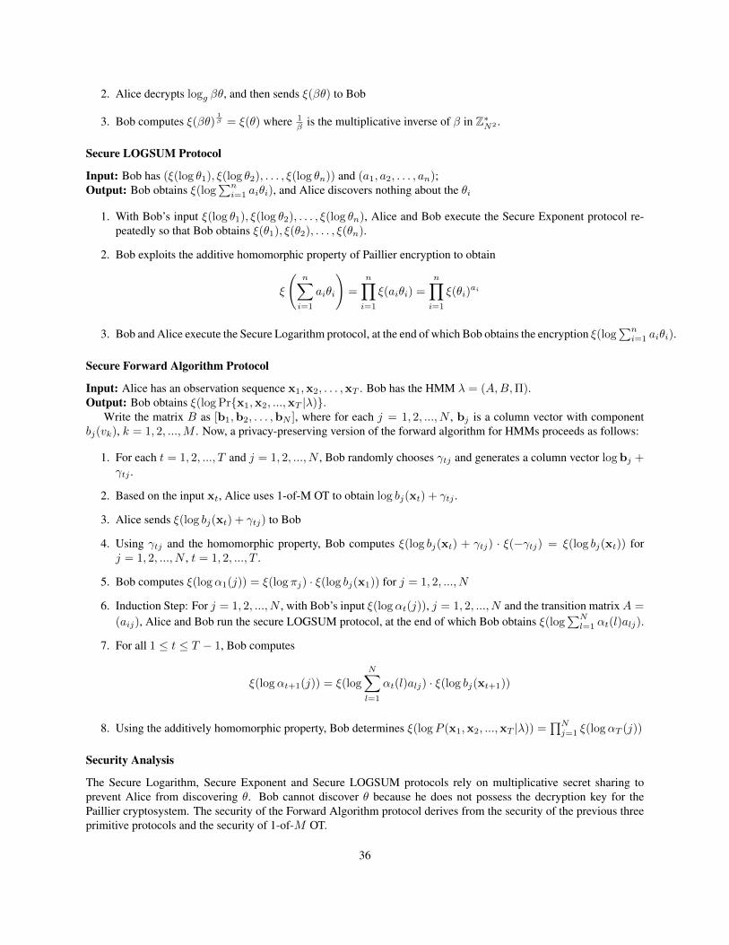
2. Alice decrypts logg βθ, and then sends ξ(βθ) to Bob

3. Bob computes ξ(βθ)1β = ξ(θ) where 1

β is the multiplicative inverse of β in Z∗N2 .

Secure LOGSUM Protocol

Input: Bob has (ξ(log θ1), ξ(log θ2), . . . , ξ(log θn)) and (a1, a2, . . . , an);Output: Bob obtains ξ(log

∑ni=1 aiθi), and Alice discovers nothing about the θi

1. With Bob’s input ξ(log θ1), ξ(log θ2), . . . , ξ(log θn), Alice and Bob execute the Secure Exponent protocol re-peatedly so that Bob obtains ξ(θ1), ξ(θ2), . . . , ξ(θn).

2. Bob exploits the additive homomorphic property of Paillier encryption to obtain

ξ

(n∑i=1

aiθi

)=

n∏i=1

ξ(aiθi) =

n∏i=1

ξ(θi)ai

3. Bob and Alice execute the Secure Logarithm protocol, at the end of which Bob obtains the encryption ξ(log∑ni=1 aiθi).

Secure Forward Algorithm Protocol

Input: Alice has an observation sequence x1,x2, . . . ,xT . Bob has the HMM λ = (A,B,Π).Output: Bob obtains ξ(log Pr{x1,x2, ...,xT |λ)}.

Write the matrix B as [b1,b2, . . . ,bN ], where for each j = 1, 2, ..., N , bj is a column vector with componentbj(vk), k = 1, 2, ...,M . Now, a privacy-preserving version of the forward algorithm for HMMs proceeds as follows:

1. For each t = 1, 2, ..., T and j = 1, 2, ..., N , Bob randomly chooses γtj and generates a column vector log bj +γtj .

2. Based on the input xt, Alice uses 1-of-M OT to obtain log bj(xt) + γtj .

3. Alice sends ξ(log bj(xt) + γtj) to Bob

4. Using γtj and the homomorphic property, Bob computes ξ(log bj(xt) + γtj) · ξ(−γtj) = ξ(log bj(xt)) forj = 1, 2, ..., N , t = 1, 2, ..., T .

5. Bob computes ξ(logα1(j)) = ξ(log πj) · ξ(log bj(x1)) for j = 1, 2, ..., N

6. Induction Step: For j = 1, 2, ..., N , with Bob’s input ξ(logαt(j)), j = 1, 2, ..., N and the transition matrixA =

(aij), Alice and Bob run the secure LOGSUM protocol, at the end of which Bob obtains ξ(log∑Nl=1 αt(l)alj).

7. For all 1 ≤ t ≤ T − 1, Bob computes

ξ(logαt+1(j)) = ξ(log

N∑l=1

αt(l)alj) · ξ(log bj(xt+1))

8. Using the additively homomorphic property, Bob determines ξ(logP (x1,x2, ...,xT |λ)) =∏Nj=1 ξ(logαT (j))

Security Analysis

The Secure Logarithm, Secure Exponent and Secure LOGSUM protocols rely on multiplicative secret sharing toprevent Alice from discovering θ. Bob cannot discover θ because he does not possess the decryption key for thePaillier cryptosystem. The security of the Forward Algorithm protocol derives from the security of the previous threeprimitive protocols and the security of 1-of-M OT.

36

Secure Keyword Recognition

Consider the following scenario for privacy-preserving keyword recognition: Alice has a sampled speech signal, whichshe converts into T frames, where each frame is represented by a 39-dimensional vector of Mel Frequency CepstralCoefficients (MFCCs). Thus Alice possesses xi, i = 1, 2, ..., T where each xi ∈ R39. Derivation of MFCCs fromspeech signals is an established practice in the speech processing literature Rabiner and Juang [1993]. Bob possesses∆ different HMMs, each trained for a single keyword. Alice and Bob will execute a secure protocol, at the end ofwhich, Alice will discover the keyword that is most likely to be contained in her speech sample.

Let d = 39. Let a d-dimensional vector y of MFCCs have a multivariate Gaussian distribution, i.e., bj(y) =N (µj ,Cj), where j = 1, 2, ..., N indexes the state of a HMM λ. Let z = [yT , 1]T . Then, log bj(y) = zTWjz,where

Wj =

− 1

2C−1j C−1

j µj

0 wj

∈ R(d+1)×(d+1)

and wj = 12µ

Tj C−1

j µj − 12 ln |C−1

j | − d2 ln 2π. The above treatment considers y to be a single multivariate Gaussian

random variable, though an extension to mixture of multivariate Gaussians is also possible. Note that the matrix Wj

is available to Bob. Further, note that log bj(y) is a linear function of products zizj where i, j ∈ {1, 2, ..., d+ 1}. Thisallows us to simplify the Secure Forward Algorithm Protocol as follows:

Simplified Secure Forward Algorithm

1. For each t = 1, 2, ..., T , Alice sets z = [xTt , 1]T . Alice sends to Bob the encryptions of all zizj with i, j ∈{1, 2, ..., d+ 1}.

2. For each HMM state j = 1, 2, ..., N , Bob obtains the encryption ξ(log bj(xt)) = ξ(zTWjz) using the additivehomomorphic property.

3. Bob executes steps 5–8 of the secure forward algorithm protocol.

Now, the protocol for secure keyword recognition is as follows.

Protocol for Secure Keyword Recognition

Input: Alice has the MFCC feature vectors x1,x2, ...,xT corresponding to her privately owned speech sample. Bobhas the database of HMMs {λ1, λ2, ..., λ∆} where each HMM λδ corresponds to a single keyword, which is denotedby τδ;Output: Alice obtains δ∗ = arg maxδ Pr{x1,x2, ...,xT|λδ}.

1. Alice and Bob execute the simplified secure forward algorithm protocol for each HMM λδ , at the end of whichBob obtains ξ(pδ) = ξ(log Pr{x1,x2, ...,xT|λδ}), δ = 1, 2, ...,∆.

2. Bob chooses an order-preserving matrix2 R = (rij)∆×∆ with random coefficients. Using the additively homo-morphic property of Paillier encryption, he computes the element-wise encryption given by (ξ(p′1), ..., ξ(p′∆)) =(ξ(p1), ..., ξ(p∆)) ·R. Bob sends the result to Alice.

3. Alice decrypts and obtains δ∗ = maxδ p′δ = maxδ pδ . This is true because R is order-preserving mapping.

4. Alice and Bob perform a 1-of-∆ OT, and Alice obtains the word τδ∗ .

2See Rane and Sun [2010] for more details

37

Computational Complexity

Let us consider the computational overhead of the protocol in terms of the number of keywords (∆), the number ofHMM states (N ), the time duration of the observation (T ) and the size of each observation (d). Alice has an overheadof O(d2T ) encryptions at the beginning of the protocol. This initial computational overhead is independent of thenumber of keywords and the size of the HMM. Bob has an overhead of O(d2N∆T ) ciphertext multiplications andexponentiations in order to determine the ξ(log bj(xt)) terms. Finally, to determine the ξ(αT (j)) terms, Alice andBob both have an overhead of O(N∆T ). Thus Alice’s protocol overhead is O((d2 + N∆)T ) while Bob’s overheadis O(d2N∆T ), which means that Bob’s overhead grows faster than Alice’s.

Practical Issues: Fixed Precision and Numerical Underflow

The Paillier cryptosystem is defined over an integer ring but the speech data consists of real numbers causing theprotocol to introduce an error in the computation. In our implementation, we used numbers accurate to 6 decimalplaces, which means that all floating point values were multiplied by a constant value 106 before encryption anddivided by the same value after decryption. Furthermore, whenever there was a floating point number in the ciphertextexponent – of the form ξ(a)b – then, the fractional part was truncated, and only the integer portion of b was used inthe calculation. These approximations introduce errors in the protocol which propagate during the iterations of theforward algorithm.

When implementing the protocol in software, another problem is that the value of αt(j) gets progressively smallerafter each iteration, and causes an underflow after a only a few iterations. This problem would not be encountered ifthe probabilities were always expressed in the form logαt(j). However, it is necessary to consider the actual valueof αt(j); the underflow problem is resolved by normalizing αt(1), . . . , αt(N) in each iteration, such that the relativevalues are preserved.

Experimental Analysis

We performed speech recognition experiments on a 3.2 GHz Intel Pentium 4 machine with 2 GB RAM and running 64-bit GNU/Linux. We created an efficient C++ implementation of the Paillier cryptosystem using the variable precisioninteger arithmetic library provided by OpenSSL. The encryption and decryption functions were used in a softwareimplementation of the protocol.

The experiment was conducted on audio samples of length 0.98 seconds each. The samples consisted of spokenwords which were analyzed by ten HMMs each having 5 states. These 10 HMMs were assumed to be trained offline(by Bob) on ten different words, viz., utterances of “one”, “two”, “three”, and so on up to “ten”. To perform speechrecognition, each test speech sample was converted into 98 overlapping vectors (called frames), a 39-dimensionalfeature vector composed of MFCCs were extracted from each overlapping vector, as is common in speech processing.These 39-dimensional vectors serve as the input observations xi owned by Alice.

The time required for processing an audio sample of length 0.98 seconds using the 10 HMMs was measured. Theresults are tabulated in Table 4.1 for the case of using 256-bit and 512-bit keys for Paillier homomorphic encryption.Using a longer key provides a stronger degree of security, but this it comes at the cost of a significant increase inprocessing time. Note that, once Bob receives the encrypted input from Alice, the calculation of ξ(log bj(xt)) for all10 HMMs can proceed in parallel. This is possible, for instance, in a cloud computing framework, where Bob hasaccess to several server nodes.

Activity 256-bit keys 512-bit keysAlice encrypts input data (only once) 205.23 s 1944.27 sBob computes ξ(log bj(xt)) (per HMM) 79.47 s 230.30 sBoth compute ξ(αT (j)) (per HMM) 16.28 s 107.35 s

Table 4.1: Protocol execution times in seconds. Note that Alice’s encryption operation occurs only once at the begin-ning of the protocol. The larger the dictionary of keywords, the larger is the computational overhead for Bob.

In order to observe the effect of error propagation, we compared the values of αT (N) for a given 0.98-second

38

speech sample derived using the the privacy preserving speech recognition protocol as well as a conventional non-secure implementation which uses no encryption. This comparison of αT (N) with and without encryption was per-formed for each of the 10 HMMs corresponding to the spoken words“one” through “ten”. The relative error in αT (N)with respect to the true values was found to be 0.5179% for both 256-bit and 512-bit Paillier encryption.

4.2.2 A framework for implementing SMC protocolsWe created a C++ framework for quickly implementing SMC protocols for machine learning and speech processingalgorithms. As we had seen before, the biggest bottleneck in implementing SMC protocols is the computational cost ofthe encryption and decryption functions and similarly, we require efficient numerical computation and linear algebrafor implementing machine learning algorithms.

SMC Framework

Cryptography

OpenSSL

Linear Algebra

BLAS LAPACK

Figure 4.7: Architecture of the SMC framework

The main computational cost of the cryptosystem comes from the variable precision arithmetic operations. Weused the variable precision arithmetic library provided by OpenSSL to implement the Paillier cryptosystem includinghomomorphic operations on the encrypted data such as modular multiplication and exponentiations of ciphertexts.Table 4.2 summarizes the time required to encrypt one number using our Paillier implementation across varying keysizes.

key size keygen 1000 encryptions # encryption/s64 bits 0.006 s 0.063 s 15873.02

128 bits 0.022 s 0.213 s 4694.84256 bits 0.174 s 1.207 s 828.50512 bits 0.644 s 8.339 s 119.92

1024 bits 42.757 s 62.907 s 15.90

Table 4.2: Encryption speeds.

We used BLAS and LAPACK libraries for fast matrix operations such as matrix inversion, multiplication, deter-minant computation. we chose to use C++ because using a native implementation of these primitives is significantlyfaster than using an virtual machine based implementation like Java or an interpreted one like Python. We chosethese libraries because they are ubiquitously available on most platforms and our framework can be used with just acompilation.

Our objective was to create an efficient framework with an high level interface which abstracts most of these detailsfrom the end developer. From our experiences in implementing SMC protocols using this framework, we believe thatit would greatly benefit the research community.

39

40

Chapter 5

Proposed Work

In this section, we describe some of the ongoing work that we propose to investigate in the scope of this thesis. Someof the work is labeled optional in the sense that we recognize them as important future directions in our research andwe hope to make progress as much as possible in the available time.

5.1 Techniques

5.1.1 Differentially Private Hidden Markov ModelsWe plan to investigate differentially private hidden Markov models (HMMs). Using this framework, it will be possiblefor a party to publish an HMM trained over private audio data. Such a release mechanism can be used as a guaranteeof privacy while collecting audio data from participants for training speech recognition systems. In general, thedifferentially private formulation will greatly simplify the SMC protocols for speech recognition. The party with thedifferentially private HMM can simply transfer the model parameters to the party with the data who can perform theHMM inference necessary for speech recognition locally without the need for any data transmission.

A continuous density HMM is constituted by a finite set of states with an emission model giving the probability ofa state emitting an observation and a transition model giving the probability of transitioning from one state to another.Our previous work on differentially private large margin GMM [Pathak and Raj, 2010b] can directly be used to modelthe emission probabilities. We can apply it in an iterative algorithm to learn the transition probabilities. Also, we planto investigate differentially private mechanisms for the large margin HMM [Sha and Saul, 2007] and other structuredclassification algorithms such as max-margin Markov networks [Taskar et al., 2003].

5.1.2 Differential Private Classification by Transforming the Loss FunctionWe have seen two mechanisms to create differentially private classifiers – the exponential mechanism [Dwork et al.,2006] and the sensitivity method [Chaudhuri and Monteleoni, 2008]. The exponential mechanism proposed by addsperturbation to the resultant optimal solution so that the classifiers trained on adjacent datasets are likely to have thesame optimum. The sensitivity method perturbs the convex objective function by a linear term to achieve the sameresult. We propose to investigate the following mechanisms.

1. Adding randomization to the data. This technique involves modifying the loss function by adding randomperturbation to the data such that the resultant classifier satisfies differential privacy. One advantage of thisapproach is that it will naturally allow multiple parties to contribute the data.

2. Kernel methods. Here we modify the loss function by adding perturbation in the kernel itself. As the dualformulation of classifiers such as support vector machines involves the kernel trick dealing with only the dotproducts, adding noise perturbing the kernel inner product should be adequate to satisfy differential privacy andwould introduce a much lower excess error.

41

In our work on differentially private classification, the ultimate goal would be to create a mechanism which pre-serves differential privacy while introducing the least amount of excess error and also to investigate under what situ-ations would such a universally optimum mechanism exist. We propose to investigate this question in the context oflarge margin classification. Our intuition is that compared to other classification algorithms, a large margin classifiershould be much more robust to perturbation.

5.1.3 Optional: Privately Training Classifiers over Data from Different DistributionsIn [Pathak et al., 2010a], we considered the problem of training a differentially private classifier by aggregating locallytrained classifiers from multiple parties. In this setting, our main assumption was that the data instances thoughbelonging to multiple parties were sampled from the same source distribution. This assumption is found to be toorestrictive in practice especially for problem areas such as speech processing as the individual characteristics of theparticipants play an important role. We aim to develop a differentially private aggregation mechanism where databelonging to each party is assumed to be sampled from different distribution.

5.2 Applications

5.2.1 Privacy Preserving Music Recognition and Keyword SpottingIn the keyword spotting involves detecting the presence of a keyword in an audio sample. A keyword is typicallymodeled as an HMM which a party can privately train using a audio dataset belonging to another party using a trainingprotocol for speech recognition as described above. Using this model, we aim to construct an SMC protocol foriterative Viterbi decoding that efficiently finds the sub-sequence an observation sequence having the highest averageprobability of being generated by a given HMM. Additionally, we can also apply some of these techniques towardsprivately searching text documents, towards creating a “private grep.”

Keyword spotting systems that use word level HMMs are analogous to HMM-based speaker identification systemsin their operation, and would require similar approaches to them privately. However, when the system permits theuser to specify the words and composes models for them from sub-word units an additional complexity is introducedif it is required that the identity of the keyword be hidden from the system. The approach will require composition ofuninformative sub-word graphs and performing the computation in a manner that allows the recipient of the result toobtain scores from only the portions of the graph that represent the desired keyword. Ezzat and Poggio [2008] proposea more fruitful approach where the keyword spotting problem is reduced to computation of correlations and a simpleSVM or boosted classifier. The approach is reportedly more accurate than the HMM-based system. Additionally, dueto its simplicity, the complexity of privacy-preserving computation is also much lower for the method.

5.2.2 Privacy Preserving Speaker Verification and IdentificationWe are interested in constructing SMC protocols for speaker identification problem, where one party – the client hasaccess to the audio data and another party – the server, wants to learn a multi-class classifier, typically, a Gaussianmixture model, to label each audio sample according to its speaker. Here are some of the issues we propose to consider.

1. SMC Protocols for Speaker Verification. In this case, the simplest systems that can be converted to privacy-preserving form are based on GMMs and HMMs. Speaker verification schemes employ a variety of “anti-speaker” and “garbage” models. Scores computed from the various models contribute to normalization schemesthat must also be incorporated securely as done by [Bimbot et al., 2004]. These normalization schemes some-times include selection of the models themselves that will used by the system. Also, in the more complexscenario, it may be desired that the user is correctly verified, but the system itself remains unaware of whoexactly was verified. To do so, the privacy-preserving framework must keep all model types active at all timesand the precise model used must not be revealed at any time.

2. SMC Protocols for Speaker Identification Given the similarity to speaker verification, the approach taken tothe development of privacy preserving speaker identification systems will also be similar. However, in this case

42

we have an additional level of complexity of requiring that the number of speakers must also be hidden. Also,the actual outcome of the identification may need to be handled differently – the intended recipient might be athird party.

3. Releasing Differentially Private Speaker Identification/Verification Classifier. The speaker identification orverification problem involves training a classifier, which is typically a Gaussian mixture model, for validatinga speaker’s identity using an audio sample. If there is such a classifier trained over private collection of speechrecordings, it can result in disclosure of information about the data. This limits the amount of analysis that canbe done on such data as well as the prospects of their auxiliary information being revealed inhibits participantsfrom contributing their audio data to such collections. Towards this, we created a mechanism for releasing adifferentially private speaker identification classifier.

5.2.3 Optional: Privacy Preserving Graph Search for Speech RecognitionWe are interested in constructing a cryptographic protocol for graph search problems. Most problems in speechrecognition including model evaluation algorithms like dynamic time warping (DTW), Viterbi decoding, as well asmodel training algorithms such as Baum-Welch can be formulated as graph search problems; an efficient protocol forprivacy preserving graph search can result in practical solutions for many of these problems.

The two specific directions we plan to investigate are:

1. Graph Traversal. We plan to study the general problem where one party has a graph and another party isinterested in performing a graph traversal privately. While this is applicable in continuous speech recognition,we also plan to apply it to the general problem of matching finite automata and regular expressions with privacyconstraints.

2. Belief Propagation. Given a graph structure, we are interested in evaluating how a potential function such asthe probability of having a contagious disease spreads across the nodes in a private manner, i.e., without anynode knowing anything about the value of the function at its neighbors. Kearns et al. [2007] present a simplifiedprivacy preserving message passing solution for undirected trees. We plan to extend it to general graphs.

5.3 Estimated TimelineWe plan to make progress towards the proposed work using the following timeline as a guide.

Time Slot TaskDec 2010 - Apr 2011 Privacy Preserving Music Matching & Keyword SpottingMay - Aug 2011 Differential Private Classification via Loss function Transformation

(optional) Differentially Private Classification from Different SourcesSep - Nov 2011 Privacy Preserving Speaker Identification/VerificationDec 2011 - Mar 2012 Differentially Private HMM

(optional) Privacy Preserving Graph SearchApr - May 2012 Dissertation writingJun 2012 Defense

43

44

Bibliography

M. Atallah and J. Li. Secure outsourcing of sequence comparisons. International Journal of Information Security, 4(4):277–287, 2005.

S. Avidan and M. Butman. Efficient methods for privacy preserving face detection. In Neural Information ProcessingSystems, pages 57–64, 2006.

B. Barak, K. Chaudhuri, C. Dwork, S. Kale, F. McSherry, and K. Talwar. Privacy, accuracy, and consistency too: aholistic solution to contingency table release. In Symposium on Principles of Database Systems, pages 273–282,2007.

D. Beaver. Foundations of secure interactive computing. In CRYPTO, pages 377–391, 1991.

M. Ben-Or, S. Goldwasser, and A. Widgerson. Completeness theorems for non-cryptographic fault-tolerant distributedcomputation. In Proceedings of the ACM Symposium on the Theory of Computing, pages 1–10, 1988.

J. Benaloh. Dense Probabilistic Encryption. In Proceedings of the Workshop on Selected Areas of Cryptography,pages 120–128, Kingston, ON, Canada, May 1994.

F. Bimbot, J.-F. Bonastre, C. Fredouille, G. Gravier, I. Magrin-Chagnolleau, S. Meignier, T. Merlin, J. Ortega-Garcia,D. Petrovska-Delacretaz, and D. Reynolds. A tutorial on text-independent speaker verification. EURASIP Journalon Applied Signal Processing, 4:430–451, 2004.

A. Blum, C. Dwork, F. McSherry, and K. Nissim. Practical privacy: The suLQ framework. In Symposium on Principlesof Database Systems, 2005.

W. Campbell. Generalized linear discriminant sequence kernels for speaker recognition. In IEEE International Con-ference on Acoustics, Speech and Signal Processing, 2002.

W. Campbell, D. Sturim, and D. Reynolds. Support vector machines using GMM supervectors for speaker verification.IEEE Signal Processing Letters, 13:308–311, 2006.

R. Canetti. Security and composition of multiparty cryptographic protocols. Journal of Cryptology, 13(1):143–202,2000.

O. Chapelle. Training a support vector machine in the primal. Neural Computation, 19(5):1155–1178, 2007.

K. Chaudhuri and C. Monteleoni. Privacy-preserving logistic regression. In Neural Information Processing Systems,pages 289–296, 2008.

K. Chaudhuri, C. Monteleoni, and A. Sarwate. Differentially private empirical risk minimization. arXiv:0912.0071v4[cs.LG], 2010.

I. Damgard and M. Jurik. A Generalisation, a Simplification and Some Applications of Paillier’s Probabilistic Public-Key System. In 4th International Workshop on Practice and Theory in Public Key Cryptosystems, pages 119–136,Cheju Island, Korea, Feb. 2001.

45

S. Davis and P. Mermelstein. Comparison of parametric representations for monosyllabic word recognition in con-tinuously spoken sentences. IEEE Transactions on Acoustics, Speech, and Signal Processing, ASSP-28(4):357,1980.

I. Dinur and K. Nissim. Revealing information while preserving privacy. In ACM Symposium on Principles ofDatabase Systems, 2003.

C. Dwork. Differential privacy. In International Colloquium on Automata, Languages and Programming, 2006.

C. Dwork and K. Nissim. Privacy-preserving datamining on vertically partitioned databases. In CRYPTO, 2004.

C. Dwork, F. McSherry, K. Nissim, and A. Smith. Calibrating noise to sensitivity in private data analysis. In Theoryof Cryptography Conference, pages 265–284, 2006.

T. Ezzat and T. Poggio. Discriminative word-spotting using ordered spectro-temporal patch features. In SAPA work-shop at Interspeech, 2008.

A. Frank and A. Asuncion. UCI machine learning repository, 2010. URL http://archive.ics.uci.edu/ml.

M. Freedman, K. Nissim, and B. Pinkas. Efficient private matching and set intersection. In Advances in Cryptology -EUROCRYPT, pages 1–19. Springer, 2004.

O. Goldreich. Foundations of cryptography: Volume II Basic Applications. Cambridge University Press, 2004.

M. Grant and S. Boyd. Graph implementations for nonsmooth convex programs. In V. Blondel, S. Boyd, andH. Kimura, editors, Recent Advances in Learning and Control, Lecture Notes in Control and Information Sciences,pages 95–110. Springer-Verlag Limited, 2008.

M. Grant and S. Boyd. CVX: Matlab software for disciplined convex programming, version 1.21. http://cvxr.com/cvx, Apr. 2010.

A. Hatch and A. Stolcke. Generalized linear kernels for one-versus-all classification: Application to speaker recogni-tion. In IEEE International Conference on Acoustics, Speech and Signal Processing, 2006.

G. Jagannathan, K. Pillaipakkamnatt, and R. N. Wright. A practical differentially private random decision tree classi-fier. In ICDM Workshop on Privacy Aspects of Data Mining, pages 114–121, 2009.

M. Kantarcioglu and C. Clifton. Privacy-preserving distributed mining of association rules on horizontally partitioneddata. IEEE Transactions on Knowledge and Data Engineering, 16(9):1026–1037, 2004.

S. P. Kasiviswanathan, H. K. Lee, K. Nissim, S. Raskhodnikova, and A. Smith. What can we learn privately? In IEEESymposium on Foundations of Computer Science, pages 531–540, 2008.

M. Kearns, J. Tan, and J. Wortman. Privacy-preserving belief propagation and sampling. In Neural InformationProcessing Systems, 2007.

P. Kenny and P. Dumouchel. Experiments in speaker verification using factor analysis likelihood ratios. In Odyssey,pages 219–226, 2004.

X. Lin, C. Clifton, and M. Y. Zhu. Privacy-preserving clustering with distributed EM mixture modeling. Knowledgeand Information Systems, 8(1):68–81, 2005.

Y. Lindell and B. Pinkas. Secure multiparty computation for privacy-preserving data mining. Journal of Privacy andConfidentiality, 1(1):59–98, 2009.

P. C. Mahalanobis. On the generalised distance in statistics. Proceedings of the National Institute of Sciences of India,2:49–55, 1936.

46

M. Naor and B. Pinkas. Oblivious transfer with adaptive queries. In Advances in Cryptology: CRYPTO, pages573–590, Seattle, USA, 1999.

P. Paillier. Public-key cryptosystems based on composite degree residuosity classes. In EUROCRYPT, 1999.

A. Papoulis. Probability, Random Variables, and Stochastic Processes. McGraw-Hill, second edition, 1984.

M. Pathak and B. Raj. Large margin multiclass Gaussian classification with differential privacy. In ECML/PKDDWorkshop on Privacy and Security issues in Data Mining and Machine Learning, 2010a.

M. Pathak and B. Raj. Large margin Gaussian mixture models with differential privacy. In IEEE Transactions onDependable and Secure Computing (submitted), 2010b.

M. Pathak and B. Raj. Privacy-preserving protocols for eigenvector computation. In ECML/PKDD Workshop onPrivacy and Security issues in Data Mining and Machine Learning, 2010c.

M. Pathak, S. Rane, and B. Raj. Multiparty differential privacy via aggregation of locally trained classifiers. In NeuralInformation Processing Systems, 2010a.

M. Pathak, S. Rane, W. Sun, and B. Raj. Privacy preserving probabilistic inference with hidden markov models. InInternational Conference on Acoustics, Speech and Signal Processing (submitted), 2010b.

J. Platt. Fast training of support vector machines using sequential minimal optimization. In Advances in KernelMethods — Support Vector Learning, pages 185–208, 1999.

M. Rabin. How to exchange secrets by oblivious transfer. Technical Report TR-81, Harvard University, 1981.

L. Rabiner and B. H. Juang. Fundamentals of Speech Recognition. Prentice-Hall, Inc., Upper Saddle River, NJ, USA,1993. ISBN 0-13-015157-2.

S. Rane and W. Sun. Privacy Preserving String Comparisons Based on Levenshtein Distance. In Proc. IEEE interna-tional Workshop on Information Forensics and Security (WIFS), Seattle, USA, Dec. 2010.

D. Reynolds. An overview of automatic speaker recognition technology. In IEEE International Conference on Acous-tics, Speech and Signal Processing, 2002.

D. Reynolds, T. Quatieri, and R. Dunn. Speaker verification using adapted Gaussian mixture models. Digital SignalProcessing, 10:19–41, 2000.

F. Sha and L. K. Saul. Large margin gaussian mixture modeling for phonetic classification and recognition. In IEEEInternational Conference on Acoustics, Speech and Signal Processing, pages 265–268, 2006.

F. Sha and L. K. Saul. Large margin hidden markov models for automatic speech recognition. In Neural InformationProcessing Systems, pages 1249–1256, 2007.

P. Smaragdis and M. Shashanka. A framework for secure speech recognition. IEEE Transactions on Audio, Speech &Language Processing, 15(4):1404–1413, 2007.

K. Sridharan, S. Shalev-Shwartz, and N. Srebro. Fast rates for regularized objectives. In Neural Information Process-ing Systems, pages 1545–1552, 2008.

B. Taskar, C. Guestrin, and D. Koller. Max-margin Markov networks, 2003.

J. Vaidya, C. Clifton, M. Kantarcioglu, and S. Patterson. Privacy-preserving decision trees over vertically partitioneddata. TKDD, 2(3), 2008a.

J. Vaidya, M. Kantarcioglu, and C. Clifton. Privacy-preserving naive bayes classification. VLDB J, 17(4):879–898,2008b.

47

J. Vaidya, H. Yu, and X. Jiang. Privacy-preserving svm classification. Knowledge and Information Systems, 14(2):161–178, 2008c.

A. Wang. An industrial strength audio search algorithm. In International Conference on Music Information Retrieval,2003.

A. Yao. Protocols for secure computations (extended abstract). In IEEE Symposium on Foundations of ComputerScience, 1982.

48

Appendix A

Proofs of Theorems and Lemmas

A.1 Privacy Preserving Eigenvector Computation (Section 4.1.1)proof of Theorem 4.1.1. We have,

MT M =

[MTM MTPPTM I

].

Multiplying by the eigenvector v =

[vt×1

v′s×1

]gives us

MT M

[vv′

]=

[MTMv +MTPv′

PTMv + v′

]= λ

[vv′

].

Therefore,

MTMv +MTPv′ = λv, (A.1)

PTMv + v′ = λv′. (A.2)

Since λ 6= 1, Equation (A.2) implies v′ = 1λ−1P

TMv. Substituting this into Equation (A.1) and the orthogonalityof P gives us

MTMv +1

λ− 1MTPPTMv =

λ

λ− 1MTMv = λv.

Hence, MTMv = (λ− 1)v.

A.2 Differentially Private Large Margin Gaussian Mixture Models (Section4.1.2)

Lemma A.2.1. Assuming all the data instances to lie within a unit `2 ball, the difference in the derivative of Huberloss function L(Φ, ~x, y) calculated over two data instances (~xi, yi) and (~x′i, y

′i) is bounded.∥∥∥∥ ∂

∂ΦcmL(Φ, ~xi, yi)−

∂

∂ΦcmL(Φ, ~x′i, y

′i)

∥∥∥∥ ≤ 2.

Proof. For notational simplicity, let us denote the difference between the distance of The derivative of the Huber lossfunction for the data instance ~xi with label yi is

∂

∂ΦcmL(Φ, ~xi, yi) =

0 if M(xi,Φc) > h,

−12h [h− ~xTi Φyi~xi − log

∑m e−~xTi Φc~xi ] e−~x

Ti Φc~xi∑

m e−~xTi

Φc~xi~xi~x

Ti if |M(xi,Φc)| ≤ h,

e−~xTi Φc~xi∑

m e−~xTi

Φc~xi~xi~x

Ti if M(xi,Φc) < −h.

49

The data points lie in a `2 ball of radius 1, ∀i : ‖~xi‖2 ≤ 1. Using linear algebra, it is easy to show that the Frobeniusnorm of the matrix ~xi~xTi is same as the `2 norm of the vector ~xi, ‖~xi~xTi ‖ = ‖~xi‖2 ≤ 1.

We have,∥∥∥∥∥ e−~xTi Φc~xi∑

m e−~xTi Φc~xi

~xi~xTi

∥∥∥∥∥ =

∥∥∥∥∥ 1

1 +∑m−1 e

−~xTi Φc~xi~xi~x

Ti

∥∥∥∥∥ =

∣∣∣∣∣ 1

1 +∑m−1 e

−~xTi Φc~xi

∣∣∣∣∣ ∥∥~xi~xTi ∥∥ ≤ 1.

The term [h − ~xTi Φyi~xi − log∑m e−~xTi Φc~xi ] is at most one when |M(~xi,Φc)| ≤ h, the Frobenius norm of the

derivative of the Huber loss function is at most one in all cases,∥∥∥ ∂∂Φcm

L(Φ, ~xi, yi)∥∥∥ ≤ 1. Similarly, for a data

instance ~x′i with label y′i, we have∥∥∥ ∂∂Φcm

L(Φ, ~x′i, y′i)∥∥∥ ≤ 1.

Finally, using the triangle inequality ‖~a−~b‖ = ‖~a+ (−~b)‖ ≤ ‖~a‖+ ‖~b‖,∥∥∥∥ ∂

∂ΦcL(Φ, ~xi, yi)−

∂

∂ΦcmL(Φ, ~x′i, y

′i)

∥∥∥∥ ≤ ∥∥∥∥ ∂

∂ΦcL(Φ, ~xi, yi)

∥∥∥∥+

∥∥∥∥ ∂

∂ΦcmL(Φ, ~x′i, y

′i)

∥∥∥∥ ≤ 2.

proof of Theorem 4.1.2. As J(Φ, ~x, ~y) is convex and differentiable, there is a unique solution Φ∗ that minimizes it. Asthe perturbation term

∑c

∑ij bijΦcij is also convex and differentiable, the perturbed objective function Jp(Φ, ~x, ~y)

also has a unique solution Φp that minimizes it. Differentiating Jp(Φ, ~x, ~y) wrt Φcm, we have

∂

∂ΦcmJp(Φ, ~x, ~y) =

∂

∂ΦcmL(Φ, ~x, ~y) + λIΦ + b. (A.3)

Substituting the optimal Φpcm in the derivative gives us

λIΦ + b = − ∂

∂ΦcmL(Φp, ~x, ~y).

This relation shows that two different values of b cannot result in the same optimal Φp. As the perturbed objectivefunction Jp(Φ, ~x, ~y) is also convex and differentiable, there is a bijective map between the perturbation b and theunique Φp minimizing Jp(Φ, ~x, ~y).

Let b1 and b2 be the two perturbations applied when training with the adjacent datasets (~x, ~y) and (~x′, ~y′), respec-tively. Assuming that we obtain the same optimal solution Φp while minimizing both Jp(Φ, ~x, ~y) with perturbationb1 and Jp(Φ, ~x, ~y) with perturbation b2,

λIΦ + b1 = − ∂

∂ΦcmL(Φp, ~x, ~y),

λIΦ + b2 = − ∂

∂ΦcmL(Φp, ~x′, ~y′),

b1 − b2 =∂

∂ΦcmL(Φp, ~x′, ~y′)− ∂

∂ΦcmL(Φp, ~x, ~y). (A.4)

We take the Frobenius norm of both sides and apply the bound on the the RHS as given by Lemma A.2.1.

‖b1 − b2‖ =

∥∥∥∥ ∂

∂ΦcmL(Φp, ~x′, ~y′)− ∂

∂ΦcmL(Φp, ~x, ~y)

∥∥∥∥=

∥∥∥∥∥n−1∑i=1

∂

∂ΦcmL(Φp, ~xi, yi) +

∂

∂ΦcmL(Φp, ~x′n, y

′n)

−n−1∑i=1

∂

∂ΦcmL(Φp, ~xi, yi)−

∂

∂ΦcmL(Φp, ~xn, yn)

∥∥∥∥∥=

∥∥∥∥ ∂

∂ΦcmL(Φp, ~x′n, y

′n)− ∂

∂ΦcmL(Φp, ~xn, yn)

∥∥∥∥ ≤ 2.

50

Using this property, we can calculate the ratio of densities of drawing the perturbation matrices b1 and b2 as

P (b = b1)

P (b = b2)=

1surf(‖b1‖)‖b1‖d exp

[− ε

2‖b1‖]

1surf(‖b2‖)‖b2‖d exp

[− ε

2‖b2‖] ,

where surf(‖b‖) is the surface area of the (d + 1)-dimensional hypersphere with radius ‖b‖. As surf(‖b‖) =surf(1)‖b‖d, where surf(1) is the area of the unit (d+ 1)-dimensional hypersphere, the ratio of the densities becomes

P (b = b1)

P (b = b2)= exp

[ ε2

(‖b2‖ − ‖b1‖)]

≤ exp[ ε

2‖b2 − b1‖

]≤ exp(ε). (A.5)

The ratio of the densities of learning Φp using the adjacent datasets (~x, ~y) and (~x′, ~y′) is given by

P (Φp|~x, ~y)

P (Φp|~x′, ~y′)=P (b = b1)

P (b = b2)

|det(J(Φp → b1|~x, ~y))|−1

|det(J(Φp → b2|~x′, ~y′))|−1, (A.6)

where J(Φp → b1|~x, ~y) and J(Φp → b2|~x′, ~y′) are the Jacobian matrices of the bijective mappings from Φp tob1 and b2, respectively. Following a procedure identical to Theorem 2 of Chaudhuri et al. [2010] (omitted dueto lack of space), it can be shown that the ratio of Jacobian determinants is upper bounded by a constant factorexp(k) = 1 + 2α

nλ + α2

n2λ2 for a constant value of α. Therefore, the ratio of the densities of learning Φp using theadjacent datasets becomes

P (Φp|~x, ~y)

P (Φp|~x′, ~y′)≤ exp(ε+ k) = exp(ε′). (A.7)

Similarly, we can show that the probability ratio is lower bounded by exp(−ε′), which together with Equation(A.7) satisfies the definition of differential privacy.

Lemma A.2.2. The objective function J(Φ) is λ-strongly convex. For 0 ≤ α ≤ 1,

J (αΦ + (1− α)Φ′) ≤ αJ(Φ) + (1− α)J(Φ′)

− λα(1− α)

2

∑c

‖Φc −Φ′c‖2.

Proof. By definition, Huber loss is λ-strongly convex, i.e.,

L (αΦ + (1− α)Φ′) ≤ αL(Φ) + (1− α)L(Φ′)

− λα(1− α)

2‖Φ−Φ′‖2 . (A.8)

where the Frobenius norm of the matrix set Φ−Φ′ is the sum of norms of the component matrices Φc −Φ′c,

‖Φ−Φ′‖2 =∑c

‖Φc −Φ′c‖2. (A.9)

As the regularization term N(Φ) is linear,

N(αΦ + (1− α)Φ′)

= λ∑cm

trace(αIΦΦcmIΦ + (1− α)IΦΦ′cmIΦ)

= αλ∑cm

trace(IΦΦcmIΦ) + (1− α)λ∑cm

trace(IΦΦ′cmIΦ)

= αN(Φ) + (1− α)N(Φ′). (A.10)

The lemma follows directly from the definition J(Φ) = L(Φ) +N(Φ).

51

Lemma A.2.3.

1

dC

[∑c

trace[IΦ(Φc −Φ′c)IΦ]

]2

≤∑c

‖Φc −Φ′c‖2.

Proof. Let Φc,i,j be the (i, j)th element of the size (d+1)×(d+1) matrix Φc−Φ′c. By the definition of the Frobeniusnorm, and using the identity N

∑Ni=1 x

2i ≥ (

∑Ni=1 xi)

2,

∑c

‖Φc −Φ′c‖2

=∑c

d+1∑i=1

d+1∑j=1

Φ2c,i,j ≥

∑c

d+1∑i=1

Φ2c,i,i

≥∑c

d∑i=1

Φ2c,i,i ≥

1

dC

(∑c

d∑i=1

Φc,i,i

)2

=1

dC

[∑c

trace[IΦ(Φc −Φ′c)IΦ]

]2

.

Lemma A.2.4.

P

[‖b‖ ≥ 2(d+ 1)2

εlog

(d

δ

)]≤ δ.

Proof. Similar to the union bound argument used in Lemma 5 in Chaudhuri and Monteleoni [2008].

A.3 Differentially Private Classification from Multiparty Data (Section 4.1.3)

Theorem A.3.1. Given a set of n training data instances lying in a ball of radius 1, the sensitivity of regularizedlogistic regression classifier is at most 2

nλ . If w1 and w2 are classifiers trained on adjacent datasets of size n withregularization parameter λ,

‖w1 − w2‖1 ≤2

nλ.

Lemma A.3.2. Let G(w) and g(w) be two differentiable, convex functions of w. If w1 = arg minw G(w) and w2 =arg minw G(w) + g(w), then ‖w1 − w2‖ ≤ g1

G2where g1 = maxw ‖∇g(w)‖ and G2 = minv minw vT∇2G(w)v for

any unit vector v ∈ Rd.

Proof of Theorem 4.1.6. We formulate the problem of estimating the individual classifiers wj and the classifier w∗trained over the entire training data in terms of minimizing the two differentiable and convex functions g(w) andG(w).

wj = argminw

J(w, x|j , y|j) = argminw

G(w),

w∗ = argminw

J(w, x, y) = argminw

L(w, x|j , y|j) +∑

l∈[K]−j

L(w, x|l, y|l) + λ‖w‖2

= argminw

J(w, x|j , y|j) +∑

l∈[K]−j

L(w, x|l, y|l) = argminw

G(w) + g(w).

52

∇g(w) =∑

l∈[K]−j

1

nl

nl∑i=1

−e−yi|lwT xi|l1 + e−yi|lwT xi|l

yixTi ,

‖∇g(w)‖ =

∥∥∥∥∥∑l

1

nl

∑i

−e−yi|lwT xi|l1 + e−yi|lwT xi|l

yixTi

∥∥∥∥∥ ≤∑l

1

nl

∥∥∥∥∥∑i

−e−yi|lwT xi|l1 + e−yi|lwT xi|l

yixTi

∥∥∥∥∥ ≤∑l

1

nl,

g1 = maxw‖∇g(w)‖ ≤

∑l

1

nl. (A.11)

∇2G(w) =1

nj

∑i

eyi|jwT xi|j

1 + eyi|jwT xi|jxi|jxi|Tj + λ1, G2 ≥ λ. (A.12)

Substituting the bounds on g1 and G2 in Lemma A.3.2,

‖wj − w∗‖ ≤ 1

λ

∑l

1

nl. (A.13)

Applying triangle inequality,

‖w− w∗‖ =

∥∥∥∥∥∥ 1

K

∑j

wj − w∗

∥∥∥∥∥∥ =1

K

∥∥∥∥∥∥∑j

wj −Kw∗

∥∥∥∥∥∥ =1

K‖(w1 − w∗) + . . .+ (wK − w∗)‖

≤ 1

K

∑j

‖wj − w∗‖ =1

Kλ

∑j

∑l∈[K]−j

1

nl=K − 1

Kλ

∑j

1

nj≤ K − 1

n(1)λ.

where n(1) = minj nj .

proof of Theorem 4.1.5. Consider the case where one instance of the training dataset D is changed to result in anadjacent dataset D′. This would imply a change in one element in the training dataset of one party and thereby achange in the corresponding learned vector wsj . Assuming that the change is in the dataset of the party Pj , the changein the learned vector is only going to be in wj ; let denote the new classifier by w′j . In Theorem A.3.1, we bound thesensitivity of wj as ‖wj − w′j‖1 ≤ 2

njελ. Following an argument similar to [Dwork et al., 2006], considering that we

learn the same vector ws using either the training datasets D and D′, we have

P (ws|D)

P (ws|D′)=

P (wj + η|D)

P(w′j + η|D′

) =exp

[n(1)ελ

2 ‖wj‖1]

exp[n(1)ελ

2 ‖w′j‖1] ≤ exp

[n(1)ελ

2‖wj − w′j‖1

]

≤ exp

[n(1)ελ

2

2

njλ

]≤ exp

[n(1)

njε

]≤ exp(ε),

by the definition of function sensitivity. Similarly, we can lower bound the the ratio by exp(−ε).

Proof of Theorem 4.1.3. We use the Taylor series expansion of the function J to have

J(ws) = J(w∗) + (ws − w∗)T∇J(w∗) +1

2(ws − w∗)T∇2J(w)(ws − w∗)

for some w ∈ Rd. By definition,∇J(w∗) = 0.Taking `2 norm on both sides and applying Cauchy-Schwarz inequality,

|J(ws)− J(w∗)| ≤ 1

2‖ws − w∗‖2 ‖∇2J(w)‖. (A.14)

53

The second gradient of the regularized loss function for logistic regression is

∇2J(w) =1

n

∑i

eyiwT xi

1 + eyiwT xixixTi + λ1 =

1

n

∑i

1

1 + e−yiwT xixixTi + λ1.

Since the logistic function term is always less than one and all xi lie in a unit ball, ‖∇2J(w)‖ ≤ λ + 1. Substitutingthis into Equation A.14 and using the fact that J(w∗) ≤ J(w),∀w ∈ Rd,

J(ws) ≤ J(w∗) +λ+ 1

2‖ws − w∗‖2. (A.15)

The classifier ws is the perturbed aggregate classifier, i.e., ws = w + η, with the noise term η ∼ Lap(

2n(1)ελ

). We

apply Lemma A.3.3 to bound ‖η‖ with probability at least 1− δ. Substituting this into Equation A.15, we have

J(ws) ≤ J(w∗) +1

2‖w− w∗ + η‖2 = J(w∗) +

λ+ 1

2

[‖w− w∗‖2 + ‖η‖2 + 2(w− w∗)Tη

]≤ J(w∗) +

λ+ 1

2

[(K − 1)2

n2(1)λ

2+

4d2

n2(1)ε

2λ2log2

(d

δ

)]+ (λ+ 1)|(w− w∗)Tη|.

Using the Cauchy-Schwarz inequality on the last term,

J(ws) ≤ J(w∗) +λ+ 1

2

[(K − 1)2

n2(1)λ

2+

4d2

n2(1)ε

2λ2log2

(d

δ

)]+ (λ+ 1)‖w− w∗‖‖η‖

≤ J(w∗) +(K − 1)2(λ+ 1)

2n2(1)λ

2+

2d2(λ+ 1)

n2(1)ε

2λ2log2

(d

δ

)+

2d(K − 1)(λ+ 1)

n2(1)ελ

2log

(d

δ

).

Proof of Theorem 4.1.8. Let wr be the classifier minimizing the true risk J(w). By rearranging the terms,

J(ws) = J(w∗) + [J(ws)− J(wr)] + [J(wr)− J(w∗)] ≤ J(w∗) + [J(ws)− J(wr)].

Sridharan, et al. Sridharan et al. [2008] present a bound between the true excess risk of any classifier as anexpression of bound on the regularized empirical risk for that classifier and the classifier minimizing the regularizedempirical risk. With probability at least 1− δ,

J(ws)− J(wr) ≤ 2[J(ws)− J(w∗)] +16

λn

[32 + log

(1

δ

)]. (A.16)

Substituting the bound from Theorem 4.1.3,

J(ws)− J(wr) ≤ 2(K − 1)2(λ+ 1)

2n2(1)λ

2+

4d2(λ+ 1)

n2(1)ε

2λ2log2

(d

δ

)(A.17)

+4d(K − 1)(λ+ 1)

n2(1)ελ

2log

(d

δ

)+

16

λn

[32 + log

(1

δ

)]. (A.18)

Substituting this bound into Equation A.16 gives us a bound on the true excess risk of the classifier ws over theclassifier w∗.

Lemma A.3.3. Given a d-dimensional random variable η ∼ Lap(β) i.e., P (η) = 12β e− ‖η‖1β , with probability at least

1− δ, the `2 norm of the random variable is bounded as

‖η‖ ≤ 2dβ log

(d

δ

).

The proof is similar to Lemma 5 of Chaudhuri and Monteleoni [2008].

54