probabilistic automated bidding in multiple auctions

Electronic Commerce Research, 5: 25–49 (2005) 2005 Springer Science + Business Media, Inc. Manufactured in the Netherlands.

Probabilistic Automated Bidding in MultipleAuctions

MARLON DUMAS and LACHLAN ALDRED {m.dumas,l.aldred}@qut.edu.auCentre for IT Innovation, Queensland University of Technology, GPO Box 2434, Brisbane QLD 4001, Australia

GUIDO GOVERNATORI [email protected] of ITEE, The University of Queensland, Brisbane QLD 4072, Australia

ARTHUR H.M. TER HOFSTEDE [email protected] for IT Innovation, Queensland University of Technology, GPO Box 2434, Brisbane QLD 4001, Australia

Abstract

This paper presents an approach to develop bidding agents that participate in multiple auctions with the goalof obtaining an item with a given probability. The approach consists of a prediction method and a planningalgorithm. The prediction method exploits the history of past auctions to compute probability functions capturingthe belief that a bid of a given price may win a given auction. The planning algorithm computes a price and a setof compatible auctions, such that by sequentially bidding this price in each of the auctions, the agent can obtainthe item with the desired probability. Experiments show that the approach increases the payoff of their users andthe welfare of the market.

Keywords: online auctions, bidding agents, bidding strategy

Following the rapid development of online marketplaces, trading practices such as dynamicpricing, auctions, and exchanges, have gained considerable momentum across a variety ofproduct ranges. In this setting, the ability of traders to rapidly gather and process marketinformation and to take decisions accordingly is becoming increasingly crucial to ensuremarket efficiency. Specifically, the ability of buyers to find the best deal for a trade de-pends on how many offers from alternative sellers they compare. On the other hand, theability of sellers to maximise their revenues depends on how many prospective buyers taketheir offers into account. Hence, the automation of offer request and comparison within adynamic environment is a common requirement for all parties.

The work reported in this paper addresses the issue of automated bid determination inonline auctions. The paper describes an approach to develop agents capable of participatingin multiple sequential or concurrent auctions, with the goal of winning exactly one of theseauctions given the following user parameters:

D: The deadline by which the item should be obtained.M: The maximum (or limit) price that the agent can bid.G: The eagerness, i.e., the minimum probability of obtaining the item by the deadline.

26 DUMAS ET AL.

The eagerness factor is a measure of the user’s risk attitude. A low eagerness factormeans that the user is willing to take the risk of not getting the item by the deadline, ifthis can allow the bidding agent to find a better price (risk-prone bidder). An eagernessfactor close to 1 means that the user wants to get the item by the deadline at any pricebelow M (risk-averse bidder). Note that we assume that the user derives no extra utilityfrom obtaining the item before the deadline: the item may be obtained at any time beforethe deadline.

The auctions in which a bidding agent participates may run in several auction houses.Each auction is assumed to be for a single unit of an item, and to have a fixed deadline. Auc-tions satisfying these conditions include First-Price Sealed-Bid (FPSB) auctions, Vickreyauctions, and fixed-deadline English auctions with or without proxy bids.1 The approachalso assumes that the bid histories of past auctions (or at least the history of final prices) areavailable. Many Web-based auction houses provide such histories. For example, eBay pro-vides several weeks of bid histories for each auction, while Yahoo! keeps up to 3 monthsof history. In addition, auction aggregators such as BidXS (www.bidxs.com) providelonger histories, although restricted to the final prices.

The approach is based on a prediction method and a planning algorithm. The predic-tion method exploits the history of past auctions in order to build probability functionscapturing the belief that a bid of a given price may win a given auction. These probabil-ity functions are then used by the planning algorithm to compute the lowest price, suchthat by sequentially bidding in a subset of the relevant auctions, the agent can obtain theitem at that price with a probability above the specified eagerness. In particular, the plan-ning algorithm detects and resolves incompatibilities between auctions. Two auctions withequal or similar deadlines are considered to be incompatible, since it is impossible to bidin one auction, wait until the outcome of this bid is known (which could be at the endof that auction), and then bid in the other auction. Given a set of mutually incompatibleauctions, the planning algorithm must choose one of them to the exclusion of the oth-ers. This choice is done in a way to maximise the winning probability of the resultingplan.

The approach takes into account that auctions may be for substitutive items with differ-ent values. The user of a bidding agent can specify a different valuation for each of therelevant auctions, and the agent uses this information when determining in which auctionsto bid and computing a bidding price. Alternatively, the user can identify a number ofattributes, and specify his/her preferences through a multi-attribute utility function.

A series of experiments based on real datasets are reported, showing that the use of theproposed approach increases the individual payoff (i.e., welfare) of the traders, as well asthe collective welfare of the market.

The rest of the paper is structured as follows. Section 1 describes the technical details ofthe approach, including the prediction and planning methods. Section 2 describes a proof-of-concept implementation and summarises some experimental results. Finally, Section 3discusses related work, and Section 4 draws some conclusions.

PROBABILISTIC AUTOMATED BIDDING IN MULTIPLE AUCTIONS 27

1. Approach

In this section, we describe the lifecycle of a probabilistic bidding agent, as well as theunderlying prediction and planning methods. We first consider the case where the agentparticipates in auctions for perfectly identical items. We then discuss how the approachhandles partial substitutes.

1.1. Overview

The bidding agent operates in 4 phases: preparation, planning, execution, and revision.

Preparation phase In the preparation phase, the agent assists the user in identifying aset of relevant auctions. Specifically, the user enters the parameters of the bidding agent(maximum price, deadline, eagerness) as well as a description of the desired item in theform of a list of keywords. Using this description, the agent queries the search enginesof all the auction houses that it knows, and displays the results. The user selects amongall the retrieved auctions, those in which the agent will be authorised to bid. The selectedauctions form what is subsequently called the set of relevant auctions. By extension, theauction houses hosting relevant auctions form the set of relevant auction houses.

For each relevant auction house, the agent gathers the bidding histories of every pastauction whose item description matches the list of keywords provided by the user. Thesebidding histories are used by the prediction method in order to build a function that givena bidding price, returns the probability of winning an auction by bidding (up to) that price.Note that the histories extracted from an auction house are only used to compute probabilityfunctions for the auctions taking place in that auction house. Thus, auctions running indifferent auction houses may have completely different probability functions.

During the preparation phase, the agent also conducts a series of tests to estimate theaverage time that it takes to execute a transaction (e.g., to place a bid or to get a quote) ineach of the auction houses in which it is likely to bid. The time that it takes to execute atransaction in an auction house a is stored in a variable δa . The value of this variable isupdated whenever the agent interacts with the corresponding auction house.

Planning phase In the planning phase, the bidding agent selects a set of auctions anda bidding price r (below the user’s maximum), such that the probability of getting thedesired item by bidding r in each of the selected auctions is above the eagerness factor.The resulting bidding plan, is such that any two selected auctions a1 and a2 have endtimes separated by at least δa1 + δa2. In this way, it is always possible to bid in an auction,wait until the end of that auction to know the outcome of the bid (by requesting a quote),and then place a bid in the next auction.

The problem of constructing a bidding plan can be formulated as follows. Given the setAa of relevant auctions, find:

• a set of auctions As ⊆ Aa , and• a real number r ≤ M (corresponding to a bidding price)

28 DUMAS ET AL.

such that:

• the end times of the auctions in As are non-conflicting, that is, for any a1 and a2 ∈ As ,|end(a2) − end(a1)| ≥ δa1 + δa2;

• the probability that at least one of the selected bids succeeds (written φ(As, r)) is greaterthan or equal to the eagerness, that is:

φ(As, r) = 1 −∏a∈As

(1 − Pa(r)

) ≥ G,

where Pa(r) is the probability that a bid of r will succeed in auction a ∈ As ;• the bidding price r is the lowest one fulfilling the above two constraints.

Should there be no r fulfilling the above constraints, the bidding agent turns back to theuser requesting authorisation to either raise M (the limit price) by the necessary amount, orto bid M in every auction in the bidding plan even though this does not yield the minimumrequired winning probability. This latter option is actually equivalent to decreasing theeargerness to that which can be achieved by making r = M . The agent can be configuredto automatically select one of the above two options without interacting with the user.

Note that by choosing the same bidding price r for every auction, the resulting biddingplan is not necessarily optimal in terms of expected utility. Indeed, in the general case,the problem of finding a bidding plan that maximises the expected utility given a budgetconstraint (i.e., maximum bidding price M) and an eagerness constraint (i.e., probabilityof winning at least G) would be formulated as follows. Find a set of auctions As ⊆ Aa ,and a bidding price for each auction in As , ra ≤ M , a ∈ As , such that:

∀a1, a2 ∈ As xa1xa2∣∣end(a2) − end(a1)

∣∣ ≥ xa1xa2(δa1 + δa2)

and

1 −∏

a∈Aa

(1 − xaPa(ra)

) ≥ G,

where xa is a 0/1 integer variable indicating whether auction a belongs in As or not (i.e.,xa = 1 if a ∈ As , 0, otherwise). The first of the above constraint encodes the time com-patibility constraints between the selected auctions, whereas the second constraint encodesthe eagerness requirement. Given these constraints, the following objective function cor-responding to the expected utility of the selected plan needs to be maximised:∑

a∈Aa

xa(M − ra)Pa(ra)∏

a′∈Aaend(a′)<end(a)

(1 − x ′

aPa′(ra′)).

In other words, the expected utility of a plan is the sum of the expected utilities for eachauction in the plan. The expected utility for an auction is the product of the payoff for thatauction (i.e., limit price minus actual bid price) times the probability of this payoff beingobtained. The probability of obtaining a payoff from an auction a is equal to the probabilityof winning auction a times the probability of losing all the auctions scheduled before a,since if one of these preceding auctions is won, the agent would not bid in auction a.


The above constrained nonlinear optimisation problem is computationally expensive tosolve. Even if we assume that the probability functions Pa are linear, the problem involvesa nonlinear objective function of degree 2(|Aa| + 1) and a nonlinear constraint of degree2|Aa| (the eagerness constraint), in addition to the linear limit price constraints and thequadratic compatibility constraints. Even worse, the problem involves 0/1 integer vari-ables and therefore has to be solved using Integer Programming (IP), which is NP-hardeven when the constraints and objective function are linear [Martello and Toth, 11]. Incontrast, by taking the simplifying assumption that the same bidding price r is bid in everyauction, our approach achieves a low complexity bound of O(|Aa| log M) as discussed inSection 1.3. In fact, what our approach does is that, instead of computing the plan whichmaximises the expected utility, it computes the plan which maximises the payoff to beobtained in the worst-case execution of the plan. Indeed, for a given plan, the payoff isguaranteed to be M − r if one of the auctions is won.

Execution phase In the execution phase, the bidding agent executes the bidding plan bysuccessively placing bids in each of the selected auctions, until one of them is successful.In the case of FPSB auctions the bidding agent places a bid of r minus the bid shavingfactor.2 In the case of Vickrey auctions and English auctions with proxy bidding, the agentplaces a proxy bid of amount r . Finally, in the case of an English auction without proxybids, the agent will place a bid of amount r just before the auction closes, since last-minutebidding is an optimal strategy in this context [Lucking-Reiley, 10; Roth and Ockenfels,13]. This latter technique can also be applied for N th-price multi-unit English auctions:the bidding agent places a last-minute bid for one unit at price r , provided that r is greaterthan the N th highest bid plus the minimum increment.

Revision phase During the execution phase, the agent periodically searches for new auc-tions matching the user’s item description, as well as for up-to-date quotes from the auc-tions in the bidding plan. Based on this information, the agent performs a plan revisionunder either of the following circumstances:

1. The user decides to insert a new auction into the relevant set.2. The current quote in one of the auctions in the bidding plan raises above r , in which

case it is no longer possible to bid r in that auction.3. The probability of winning given the remaining portion of the bidding plan (i.e., given

the set of remaining auctions) drops below the revision threshold which is defined asthe eagerness multiplied by the revision factor discussed below. This can occur eitherbecause the number of remaining auctions has significantly decreased since the timethat the plan was constructed, or because the current quotes in the remanining auctionshave increased, which has the effect of decreasing the probability of winning in each ofthese auctions with a bid of r .

The revision factor is a configuration parameter of the bidding agent. It is a real numberbetween 0 and 1. A revision factor equal to 1 means that the revision threshold is equalto the eagerness, which in turn means the agent will perform a plan revision after everyauction to ensure that the probability of winning is equal to the eagerness throughout the

30 DUMAS ET AL.

bidding process.3 A revision factor equal to zero implies that the revision threshold is equalto zero, which in turn means that no plan revision will occur due to the revision thresholdbeing broken, although a plan revision may still be triggered in response to the first or thesecond revision events outlined above.

The need for the revision factor stems from the fact that there are two possible interpre-tations of the concept of eagerness. The first interpretation is that an eagerness factor G

means that the user wishes to have a probability G of winning at each time point duringthe bidding process (even when most auctions have already been lost). A second interpre-tation is that an eagerness factor G means that the user wishes to have a probability G ofwinning when looking at the bidding process as a whole (from beginning to end). Eitherinterpretation can be captured by setting the revision factor to one or to zero, respectively.Intermediate behaviours can be achieved by setting the revision factor to another number.

Should a plan revision be required, the agent updates the set of relevant auctions andthe bidding histories according to any new data, and re-enters the planning phase. Oncea new bidding plan is computed, the agent returns to the execution phase. Although thealgorithms used in the execution phase are efficient, it may happen that during the planningphase following a revision event, the deadlines of some of the ongoing auctions expire. Ifthe agent detects that this can occur, it will place a bid in the auctions which are about toexpire, without waiting for the plan re-computations to complete.

Note that if the revision factor is greater than zero, the bidding price r is likely to increaseduring the bidding process. Specifically, the agent will start with a low bidding price, and itwill increase it as needed in order to maintain the probability of winning above the revisionthreshold.

1.2. Prediction methods

We propose two methods that a bidding agent can use to construct a probability functiongiven the bidding histories of past auctions. Both methods operate differently in the case ofFPSB, than they do in Vickrey and English auctions. This is because in an FPSB auction,the final price of an auction reflects the valuation of the highest bidder (after factoring bidshaving), whereas in a Vickrey or in an English auction, the final price reflects the valuationof the second highest bidder.

1.2.1. The case of FPSB auctions The first prediction method, namely the histogrammethod, is based on the idea that at the beginning of an auction, and assuming a zeroreservation price, the probability of winning with a bid of z, is equal to the number oftimes that the agent would have won had it bid z in each of the past auctions, divided bythe total number of past auctions. As the auction progresses, this probability is adjusted insuch a way that when the current quote is greater than z, the probability of winning with abid of z is zero.

Formally, we define the histogram of final prices of an auction type, to be the functionthat maps a real number x, to the number of past auctions of that type (same item, sameauction house) whose final price was exactly x. The final price of an auction a with no bids


and zero reservation price, is then modelled as a random variable fpa whose probabilitydistribution, written P(fpa = x), is equal to the histogram of final prices of the relevantauction type, modified to include the bid shaving factor, and scaled down so that its totalmass is 1. The probability of winning an auction with a bid of z assuming a null reservationprice, is given by the cumulative version of this distribution, that is:

P(fpa ≤ z) =∑

0≤x≤z

P (fpa = x)

given an appropriate discretisation of the interval [0, z]. For example, if the sequence ofobserved final prices (after including the bid shaving factor) is [22, 20, 25], the cumulativedistribution at the beginning of an auction is:

Pa(z) = P(fpa ≤ z) =

1 for z ≥ 25,0.66 for 22 ≤ z < 25,0.33 for 20 ≤ z < 22,0 for z < 20.

In the case of an auction a with quote q > 0 (which is determined by the reservationprice and the public bids), the probability of winning with a bid of z is:

Pa(z) = P(fpa ≤ z | fpa ≥ q) = P(fpa ≤ z ∧ fpa ≥ q)

P (fpa ≥ q)=

∑q≤x≤z P (fpa = x)∑x≥q P (fpa = x)

.

In particular, Pa(z) = 0 if z < q , and if z > q , the probability of the final price beingequal to z decreases as z approaches q .

The histogram method has three drawbacks. First, the complexity of the computationof the value of the cumulative distribution is dependent on the size of the history. Giventhat the bidding agent heavily uses this function, this creates some computational overheadwhen large histories are involved. Second, the histogram method assumes that the probabil-ity of winning remains constant between two observed final prices. This is counter-intuitivesince one would expect that a higher bid always leads to a higher probability of winning.Third, the method is inapplicable if the current quote of an auction is greater than all thefinal prices of past auctions, since the denominator of the above formula is then equal tozero. Intuitively, the histogram method is unable to extrapolate the probability of winningan auction if its current quote has never been observed in the past. To avoid these two latterdrawbacks, linear interpolation could be applied between every two consecutive points inthe cumulative histogram distribution. In the above example, this would mean that Pa(z)

would linearly increase from 0 for z = 0 to 0.33 for z = 20, then continue to increasewith a different slope for 20 ≤ z ≤ 22, and so on. Although this solves the above issueswith a small additional computational overhead, one could argue whether linear interpola-tion provides an appropriate way of approximating the underlying probability distribution,or whether more appropriate approximations could be sought, with the same or even lesscomputational overhead.

The normal method is an alternative to the histogram method, which avoids its draw-backs at the price of a more restricted scope of applicability. Assuming that the number ofpast auctions is large enough (more than 50), if the final prices of these auctions follow a

32 DUMAS ET AL.

normal distribution with mean µ and standard deviation σ , then the random variable fpa

can be given the normal distribution N(µ, σ). The probability of winning with a bid z inan auction a with no bids and zero reservation price, is then given by the value at z of thecorresponding cumulative normal distribution:

Pa(z) = P(fpa ≤ z) = 1√2πσ

∫ (z−µ)/σ

−∞e−x2/2dx.

Meanwhile, if the current quote q of an auction a is greater than zero, the probability ofwinning this auction with a bid of z is:

Pa(z) = P(fpa ≤ z | fpa ≥ q) = P(fpa ≤ z ∧ fpa ≥ q)

P (fpa ≥ q)=

∫ (z−µ)/σ

(q−µ)/σ e−x2/2dx∫ ∞(q−µ)/σ

e−x2/2dx.

Many fast algorithms for approximating the integrals appearing in these formulae aswell as their inverses are described in [Thisted, 18]. The complexity of these algorithms isonly dependent on the required precision, not on the size of the dataset from which µ andσ are derived. Hence, the normal method can scale up to large sets of past auctions.

In support of the applicability of the normal method, it can be argued that the finalprices of a set of auctions for a given item are likely to follow a normal distribution, sincethe item has a more or less well-known value, around which most of the auctions shouldfinish. An analysis conducted over datasets extracted from eBay and Yahoo! (two of thesedatasets are described in Section 2) was performed to validate this claim. The final pricesof 4 histories of auctions were tested for normality using the D’Agostino–Pearson test[D’Agostino et al., 5]. The results were consistently positive for all prefixes of more than50 elements of these histories.

More generally, any method for estimating probability distributions of real random vari-ables given a set of observed values could be used for estimating the final prices of futureauctions. The histogram method, and its variant using linear interpolation, are just simpleexamples of such methods. In the case of long histories of auctions, (e.g., several months)a method that takes into account data aging could be more appropriate. Other methodswhich have been experimentally shown to provide good estimations with small amountsof seed data have been proposed in [Schapire et al., 15]. These methods work under theassumption that the observed values are drawn from identical independent distributions: areasonable assumption in the context of auction-based markets.

1.2.2. The case of English and Vickrey auctions In the case of FPSB auctions, theprediction methods assume that the probability of winning with a given bid can be derivedfrom the final prices of past auctions. This is valid since in FPSB auctions, the final priceof an auction (after factoring bid shaving and assuming that bidders are rational) is equalto the maximum price that the highest bidder was willing to pay, so that the final pricesobserved in an auction’s bid history can be directly used to predict up to how much willbidders bid in future auctions.

In the case of a Vickrey or in English auction, however, the final price of an auction doesnot reflect the limit price that the highest bidder was willing to pay (i.e., his/her valuation),


but rather the limit price of the second highest bidder. If the prediction methods describedabove were applied directly to a history of final prices of Vickrey and/or English auctions,the result would be that the bidding agent would be competing against the second highestbidders, rather than against the highest ones. In order to make the prediction methodspreviously described applicable to Vickrey and English auctions, we need to map a set ofbidding histories of Vickrey or English auctions, into an equivalent set of bidding historiesof FPSB auctions. This means that we need to extrapolate how much the highest bidder waswilling to pay in an auction, knowing how much the second highest bidder (and perhapsalso other lower bidders) was/were willing to pay.

We propose the following simple extrapolation technique. First, the bidding histories ofall the past auctions are considered, in turn, and for each of them, a set of known valuationsis extracted. The highest bid in a Vickrey auction or in an English-Proxy auction is takenas being the known valuation of the second highest bidder of that auction. The same holdsin an English auction without proxy bids, provided that there are no last minute bids (i.e.,no auction sniping). Indeed, in the absence of last minute bids, one can assume that thesecond highest bidder had the time to outbid the highest bidder, but did not do so because(s)he had reached his valuation. Similarly, it is possible under some conditions to deducethe valuation of the third highest bidder, and so on for the lower bidders.

Next, the set of known valuations of all the past auctions are merged together to yielda single collection of values, from which a probability distribution is built using either ahistogram method, a normal method, or any other appropriate statistical technique. In anycase, the resulting distribution, subsequently written Dv , takes as input a price, and returnsthe probability that there is at least one bidder willing to bid that price for the desired item.

Finally, for each auction a in the set of past auctions, a series of random numbers aredrawn according to distribution Dv , until one of these numbers is greater than the observedfinal price of auction a. This number is then taken to be the valuation of the highest bidder,which would have been the auction’s final price had the auction been FPSB and has everybidder bid his/her valuation. By applying this procedure to each past auction in turn, ahistory of “extrapolated” final prices is built. This extrapolated history is used to build anew probability distribution using the methods previously described in the setting of FPSBauctions. In other words, an extrapolated history built from a set of Vickrey or Englishauctions, is taken to be equivalent to a history of final prices of FPSB auctions.

This method for extrapolating the history of final prices of English and Vickrey auctionsis not unique. Extrapolation techniques based on other distributions than the normal onecan be designed. However, the experimental results discussed in Section 2 show that theproposed method produces a probability distribution that, when used by a probabilitisticbidding agent, yields appropriate estimations.

1.3. Planning algorithms

The decision problem that the bidding agent faces during its planning phase (see Sec-tion 1.1), is that of finding the lowest r such that there exists a set of relevant auctions As ,such that φ(As, r) ≥ G. By observing that for any auction a, the function Pa is monoton-

34 DUMAS ET AL.

ically increasing, we deduce that φ(A, x) is also monotonically increasing on its secondargument. Hence, searching the lowest r such that φ(As, r) ≥ G can be done througha binary search. At each step during this search, a given r is considered. An optimisa-tion algorithm BestPlan outlined below is then applied to retrieve the subset As ⊆ Aa

such that φ(As, r) is maximal. If the resulting φ(As, r) is between G and G + ε (ε be-ing the precision at which the minimal r is computed), then the search stops. Otherwise,if φ(As, r) > G + ε (respectively φ(As, r) < G), a new iteration is performed with asmaller (respectively greater) r as per the binary search principle. The number of itera-tions required to minimise r is logarithmic on the size of the range of r , which is M/ε. Ateach iteration, the algorithm BestPlan is called once. Thus, the complexity of the planningalgorithm is O(log(M/ε) · complexity(BestPlan)).

Given a bidding price r , the problem of retrieving the subset As ⊆ Aa with maximalφ(As, r), can be mapped into a graph optimisation problem. Each auction is mapped intoa node of a graph. The node representing auction a is labeled with the probability oflosing auction a by bidding r , that is: 1 − Pa(r). An edge is drawn between two nodesrepresenting auctions a1 and a2 iff a1 and a2 are compatible, that is:

∣∣end(a2) − end(a1)∣∣ ≥ δa1 + δa2,

where δa1 (δa2) is the connection time to auction a1 (a2), as discussed in Section 1.1.The edge goes from the auction with the earliest end time to that with the latest end time.

Given this graph, the problem of retrieving a set of mutually compatible auctions such thatthe probability of losing all of them (with a bid of r) is minimal, is equivalent to the criticalpath problem [Cormen et al., 4]. Specifically, the problem is that of finding the path in thegraph which minimises the product of the labels of the nodes. The classical critical pathalgorithm has a complexity linear on the number of nodes plus the number of edges. In theproblem at hand, the number of nodes is equal to the number of auctions, while the numberof edges is (in the worst case) quadratic on the number of auctions. Hence, the complexityof the resulting BestPlan algorithm is O(|Aa|2). More details about this algorithm can befound in [Dumas et al., 6].

An alternative algorithm with linear complexity can be devised in the case where allthe auctions are equally reachable (i.e., they all have the same δa). In this situation, thefollowing property holds:

∀a1, a2, a3 ∈ Aa end(a3) ≥ end(a2) ≥ end(a1) ∧ a3 compatible with a2

⇒ a3 compatible with a1.

Given this property, it is possible to find the best plan as follows. The set Aa , sorted byend times, is scanned once. At each step, the best predecessor of the currently consideredauction is incrementally computed. Specifically, the best predecessor of the current auc-tion is either the best predecessor of the previous auction, or one of the auctions which arecompatible with the current auction and not compatible with the previous auction. Thisincremental computation takes constant time when amortised over the whole set of itera-tions. For example, consider Table 1. Assuming that δa = 1 for all auctions, the best pathfor this set of auctions is the sequence [1, 2, 5, 6] and the associated probability of winning


Table 1. Sample array of auctions with end times and probability of winning.

Auction # 1 2 3 4 5 6

End time 4 7 8 11 12 14Win probability 0.8 0.8 0.7 0.8 0.9 0.9

is 1 − (1 − 0.8)2(1 − 0.9)2 = 0.9996. This path can be found by sequentially scanning thesequence of auctions sorted by end times. When auction 4 is reached, the choice betweenbidding in auctions 2 and 3 (which are incompatible) is made. Similarly, when auction 6is reached, the choice between auctions 4 and 5 is made. The resulting linear-complexityalgorithm BestPlan′ is given in Appendix A.

1.4. The case of partial substitutes

Hitherto, we have assumed that the user values all the auctioned items in the same way. Inreality, however, it is often the case that the characteristics of the items sold in an auctionhouse differ from one auction to another, even when the items belong to the same category.For example, two auctions might both concern new mobile phones of a given brand andmodel. However, in one of the auctions, the phone is locked to a given network (e.g.,AT&T), while in the other it is unlocked. Or in one auction, the phone comes with a 1-yearwarranty, while in the other there is no warranty. As a result, the user might be willingto pay more in one of the auctions than (s)he would in the other, although winning anyof the two auctions satisfies his/her requirements. Two items which are considered to besubstitutive by the user, but have different values, are said to be partial substitutes. Ourproposal handles partial substitutes in either of two ways: through price differentiationor through utility differentiation. Both approaches assume that the user’s value functionis linear: a very frequent assumption in the area of preference modelling for comparativeshopping [Tewari and Maes, 17].

In the price differentiation approach, the user specifies a limit price for each relevant auc-tion. The agent uses these limit prices to compute relative valuations between the auctions.For example, if the user specifies a limit price of 100 in auction A1, and 80 in auction A2,A2 is said to have a relative valuation of 80% with respect to A1. Consequently, the agentwill prefer bidding $70 in A1 rather than bidding $60 in A2 (since 0.8 · 70 ≤ 60), but itwill prefer bidding $60 in A2, rather than $80 in A1 (since 60 ≤ 0.8 · 80). More generally,given a set of relevant auctions A1, . . . , An with limit prices M1, . . . ,Mn, the agent com-putes a set of proportionality factors W1, . . . ,Wn, such that Wi = Mi/ max(M1, . . . ,Mn).The proportionality factor Wi of auction Ai is the relative importance of Ai with respectto the auction(s) with the highest limit price. During the planning phase, whenever the al-gorithm BestPlan (or BestPlan′) would consider the possibility of placing a bid of x in anauction Ai , the algorithm considers instead the possibility of placing a bid of x · Wi (line 6of algorithm BestPlan′, Appendix A). As a result, higher bidding prices are considered forauctions with higher limit prices. Accordingly, during the execution phase, if the biddingprice computed during the planning phase is r , the agent places a bid of r ·Wi in auction Ai .

36 DUMAS ET AL.

The utility differentiation approach is based on Multi-Attribute Utility Theory (MAUT).Concretely, the user identifies a set of criteria for comparing auctions (e.g., price, quality,seller’s reputation, and warranty), and specifies a weight for each criterion (e.g., 50% forthe price, 20% for the quality, 20% for the seller’s reputation, 10% for the warranty). Next,for each relevant auction and for each criterion (except the price), the user manually orthrough some automated method provides a score: a rating of the auctioned item withrespect to the considered criterion. Finally, the user specifies the limit price that (s)he iswilling to bid in any auction (called M).

Given all the scores and weights, the agent computes for each auction Ai , a utility exprice Ui = ∑

wjsj , where wj denotes the weight of criterion Cj , and sj denotes the scoregiven to criterion Cj in auction Ai (the sum is done over all the criteria except the price).The limit price Mi to pay in auction Ai is defined as:

Mi = M(1 − (1 − wp)(Umax − Ui)

),

where wp is the weight given by the user to the price (thus 1 − wp is the weight given to allthe other criteria), and Umax is the maximum element in the set {U1, . . . , Un}. In particular,for an auction with maximal utility ex price, the limit price is M . For an auction with non-maximal utility ex price, the limit price is lower than M by an amount proportional tothe difference between the highest valuation ex price, and the valuation ex price of thatauction. The weight given by the user to the price (i.e., wp) acts as a gearing factor inthis proportionality: the lower wp, the higher the amount that will be taken off from M todetermine the limit price of an auction with non-maximal utility.

Once the set of limit prices {M1, . . . ,Mn} of each auction has been computed, the bid-ding agent applies the price differentiation approach (see above).

2. Experiments

In order to validate the benefits of the probabilistic bidding approach, we conducted a seriesof experiments in which a number of probabilistic bidding agents, and a number of biddingagents implementing a simple approach, were put together in a simulated auction market.

2.1. Elements of the experimental setup

Seed data. Datasets obtained from eBay were used as a “seed” to create simulated auc-tions. Specifically, two sets of bidding histories were collected. The first dataset contained300 auctions for new PalmVx PDAs over the period 17 June 2001–15 July 2001. Thesecond dataset contained 100 auctions for new Nokia 8260 cellular phones over the period13 June 2001–31 July 2001. The choice of the datasets was motivated by the high numberof overlapping auctions that they contained.

Control bidder. A control bidding agent (also called a control bidder) is a simple agentthat simulates the presence of a human bidder in one auction. A control bidder is assigned a


limit price, and it places a (proxy) bid with this price at some point during its lifecycle. Thelimit price of a control bidder is generated randomly based on the seed data. Specifically,the average and standard deviation of the final prices of the auctions in the seed data areused to build a random number generator with a normal distribution, and this generatoris used to assign limit prices to control bidders. The adjective “control” comes from thefact that the set of control bidders acts as a “control group” with respect to which theperformance of the probabilistic bidders (see below) is measured.

A major difference between a control bidder and a human bidder is that when a humanbidder loses an auction, (s)he is likely to place a bid in another auction later. This behaviourcan be taken into account by having a consistent number of control bidders in every auction,the assumption being that N control bidders assigned to N auctions simulate the behaviourof a human that places successive bids in these N auctions.

Probabilistic bidder. An agent implementing the approach proposed in this paper.A probabilistic bidder has a limit price, an eagerness, and a deadline. The normal pre-diction method and the optimised planning algorithm were used. The revision factor wasset to zero, meaning that we took the interpretation in which a probabilistic bidder witheagerness G has a probability G of winning when looking at the bidding process as awhole. Also, all items were considered to be identical (no partial substitutes). Simulatinga marketplace with partial substitutes is a subject for a separate work.

Auction house. A software package providing the functionality of an online auction housesuch as creating an auction, processing a bid, providing a quote, or providing the historyof past auctions for a given item. All these functionalities were encapsulated in a Javapackage designed to work as an RMI server.

Simulated auctions. A simulated auction runs within an auction house. In the experi-ments, there was a one-to-one correspondence between a “real” auction recorded in theseed data, and a simulated auction. The period of time during which a simulated auc-tion ran was obtained by scaling down and offsetting the period of time during which thecorresponding “real” auction occurred. All simulated auctions were English with proxybidding.

Simulation. A simulation is a set of simulated auctions in which control bidders andprobabilistic bidders compete to obtain a given type of item. A simulation involves thefollowing steps:

1. The creation and initialisation of an auction house and a number of simulated auctions.Each simulated auction is generated from a real auction as recorded in a dataset.

2. The creation of a number of control bidders for each auction.3. The creation of a number of probabilistic bidders in the middle of the simulation. The

percentage of auctions that are allowed to complete before creating a given probabilisticbidder is called the agent’s creation time.

Accordingly, the main parameters of a simulation are:

38 DUMAS ET AL.

• dataset: the seed data.• numControls: number of control bidders competing in each auction.

In addition, each probabilistic bidding agent in a simulation is given the following para-meters:

• limitPrice: the agent’s limit price.• eagerness: the agent’s eagerness.• creationTime: the agent’s creation time. The agent will start bidding as soon as possible

after its creation time, and until the end of the simulation (which acts as its deadline). Inthe experiments, we set the creation time to be equal to 0.5, so that when the probabilisticbidder(s) enter the market, there are enough bid histories on which they can rely.

Simulation bundle. A group of simulations with identical parameters. The number ofsimulations composing a bundle is given by the parameter numSims. In addition to thisparameter, a simulation bundle has exactly the same parameters as a single simulation.

2.2. Claims, experiments, and results

Claim 1 (Correctness). The percentage of times that a probabilistic bidder succeeds toobtain an item is equal to its eagerness.

To validate this claim, we conducted an experiment consisting of 14 simulation bundles:each one designed to measure the percentage of wins of one probabilistic bidder with agiven eagerness. The eagerness was varied between 30% and 95% at steps of 5%. Theother parameters of the simulation bundles were: numSims = 50, dataset = PalmVx,numControls = 3, limitPrice = 300, creationTime = 0.5.4 For this experiment, the limitprice of the probabilistic bidders was 10 standard deviations above the average winningprice, so that there was little risk that the agent failed due to an insufficient limit price.

The expected result was that the percentage of wins is equal to the eagerness. The linearregression of the experimental results supports the claim (Figure 1): it shows an almostperfect correlation between an increase in eagerness and an increase in the percentage ofwins.

Interestingly, the fact that the bidding histories of English auctions are adjusted beforebeing used to compute a probability function (see Section 1.2.2), plays a crucial role inensuring that the percentage of wins is equal to the eagerness. We conducted the sameexperiment as above without adjusting the bidding histories. The result was that the per-centage of wins was consistently lower than the eagerness, meaning that the expectationsof the user were not fulfilled.

We also conducted experiments to observe the correlation between the average winningprice of the probabilistic bidder and its eagerness. The results show an increase of the pricepaid by the probabilistic bidder as the eagerness is increased (Figure 2).


Figure 1. Results of experiments for claim 1. Each point denotes the percentage of times that the probabilisticbidder won in a simulation bundle. The straight line is the linear regression of the plotted points.

Figure 2. Variation of a probabilistic bidder’s bid price with increasing eagerness.

40 DUMAS ET AL.

Figure 3. Results of experiments for Claim 2. Each pair of columns show the average price paid per simulationbundle. The left columns correspond to the probabilistic bidders’ average winning price; the right columnscorrespond to the control bidders’ average winning price.

Claim 2 (Increased payoff). Probabilistic bidders pay less than control bidders, especiallyin competitive environments. In other words, probabilistic bidders increase the payoff oftheir users.

To validate this claim, we conducted an experiment consisting of 7 simulation bundles:each testing the performance of one probabilistic bidder competing against control biddersin an increasingly competitive market. The number of control bidders per auction wasvaried from 2 to 8. The parameters passed to the simulations included: dataset = PalmVx,numSims = 50, eagerness = 0.9, creationTime = 0.5.

The expected results were (i) that the increasing competition raises the average finalprice of the auctions, and (ii) that despite the increased competition the probabilistic biddertends to keep its bidding price low. The actual experimental results (Figure 3) clearly matchthese expectations. Other experiments with different eagerness yielded similar results.

Claim 3 (Increased welfare). The welfare of the market increases with the number ofprobabilistic bidders.

The market welfare is a measure of the “quality” of the allocation between buyers andsellers resulting from the auctioning process. It is defined as the sum of the welfares ofthe bidders plus the sum of welfares of the sellers. The welfare of a seller is in turn de-fined as the difference between the price at which (s)he actually sells its item, and his/herreservation price. The welfare of a bidder (whether probabilistic or control) is the differ-ence between his/her limit price, and the price actually paid. If a bidder does not win anyauction, it does not contribute to the market welfare. A similar remark applies for sellerswhose auctions are not won by any bidder.


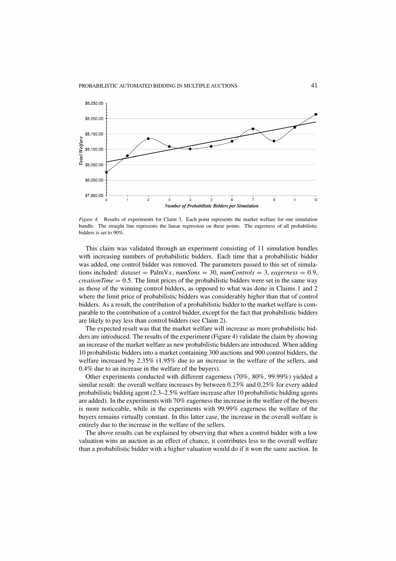
Figure 4. Results of experiments for Claim 3. Each point represents the market welfare for one simulationbundle. The straight line represents the linear regression on these points. The eagerness of all probabilisticbidders is set to 90%.

This claim was validated through an experiment consisting of 11 simulation bundleswith increasing numbers of probabilistic bidders. Each time that a probabilistic bidderwas added, one control bidder was removed. The parameters passed to this set of simula-tions included: dataset = PalmVx, numSims = 30, numControls = 3, eagerness = 0.9,creationTime = 0.5. The limit prices of the probabilistic bidders were set in the same wayas those of the winning control bidders, as opposed to what was done in Claims 1 and 2where the limit price of probabilistic bidders was considerably higher than that of controlbidders. As a result, the contribution of a probabilistic bidder to the market welfare is com-parable to the contribution of a control bidder, except for the fact that probabilistic biddersare likely to pay less than control bidders (see Claim 2).

The expected result was that the market welfare will increase as more probabilistic bid-ders are introduced. The results of the experiment (Figure 4) validate the claim by showingan increase of the market welfare as new probabilistic bidders are introduced. When adding10 probabilistic bidders into a market containing 300 auctions and 900 control bidders, thewelfare increased by 2.35% (1.95% due to an increase in the welfare of the sellers, and0.4% due to an increase in the welfare of the buyers).

Other experiments conducted with different eagerness (70%, 80%, 99.99%) yielded asimilar result: the overall welfare increases by between 0.23% and 0.25% for every addedprobabilistic bidding agent (2.3–2.5% welfare increase after 10 probabilistic bidding agentsare added). In the experiments with 70% eagerness the increase in the welfare of the buyersis more noticeable, while in the experiments with 99.99% eagerness the welfare of thebuyers remains virtually constant. In this latter case, the increase in the overall welfare isentirely due to the increase in the welfare of the sellers.

The above results can be explained by observing that when a control bidder with a lowvaluation wins an auction as an effect of chance, it contributes less to the overall welfarethan a probabilistic bidder with a higher valuation would do if it won the same auction. In

42 DUMAS ET AL.

other words, the fact that probabilistic bidders participate in as many auctions as they can,makes them likely to contribute to an increase in the overall welfare by “stealing” auctionsthat would otherwise go to bidders with lower valuations. In addition, when several proba-bilistic bidders compete in the same auctions, the market becomes more competitive. This,in turn, has a positive effect on the welfare of the sellers who get better prices than theywould in the absence of probabilistic bidders.

The observed increase in welfare is therefore explained by the “systematic” approachadopted by probabilistic bidders: a characteristic that is independent of the eagerness fac-tor. Even probabilistic bidders with an eagerness of 99.99%, which tend to select biddingprices r close to their maximum M from the very beginning of their lifespan, contributeto an increase in the overall welfare by pushing the final prices up, thereby increasing thesellers’ welfare while keeping the buyers’ welfare constant. When the eagerness factor ofthe probabilistic bidders is smaller (e.g., 70%), an increase in the buyers’ welfare can alsobe observed, since some probabilistic bidders win auctions with prices r well below theirvaluation M , thereby contributing M − r price units to the buyers’ welfare.

3. Related work

Commercial bidding tools Auction aggregators such as BidXS, BidFind (www.bidfind.com), and AuctionBeagle (www.auctionbeagle.com) address the issueof searching auctions for a given type of item across multiple auction houses. In BidXS forexample, a user enters a list of keywords, a time-frame, and a price range, and the web siteretrieves ongoing auctions running in a number of auctions houses, that match the specifiedcriteria. The resulting pages contain a list of auctions with their descriptions, end times andcurrent quotes. This list can be refreshed to obtain up-to-date quotes.

In association with StrongNumbers, BidXS also provides a service through which userscan retrieve the prices of past transactions for a given item. This service lists a largeset of items arranged by categories and provides for each of these items, a histogram oftransaction prices. Based on these histograms, the service recommends a “fair value” foreach item. This service partially addresses the “how much” part of the bid planning aspect.

Automated bid placement in Internet auction houses is currently limited to proxy biddingin English auctions. In proxy bidding, the user discloses to the auction house the maximumamount that (s)he is willing to bid in an auction. Subsequently, each time that the user isoverbid, the system places a bid on the user’s behalf up to the authorised amount. Proxybidding allows a user to continuously hold the maximum bid in an auction. However, itdoes not allow a user to hold the maximum bid in one among a set of alternative auctions,which is the subject of this article.

Another form of automated bid placement has been offered for many years by auctionsniping services such as PhantomBidder (www.phantombidder.com), Cricket Sniper(www.cricketsniper.com), and AuctionStealer (www.auctionstealer.com).Using these services, a user can schedule a bid to be placed in a given auction a few secondsbefore its closing time. If the holder of the highest bid has not placed a proxy bid higher


than his/her current bid, such a last-minute bid allows a trader to win the auction at a lowerprice than what a normal competition would allow.

PhantomBidder also offers a “Group Bidding” service. Using this service, the user canmark a number of auctions as belonging to the same group. Once a group has been formed,the user instructs the server to sequentially bid in each of the auctions in the group with thegoal of winning one of them. The price at which the service will bid is set by the user on anauction-by-auction basis. The service automatically places bids at the right moment usingits auction sniping technique and using proxy bidding where available. As soon as one ofthe bids succeeds, the service stops and sends a notification to the user. Group biddingdiffers from our approach in several ways. First, in group bidding, the user must detect andresolve potential conflicts between auction deadlines, whereas in our approach this is doneby the bidding agent. Second, in group bidding the user must manually factor in his/herattitude towards risk when determining that bidding price for each auction (each biddingprice must be entered manually). In our approach on the other hand, the user just sets amaximum price and an eagerness factor, and the bidding agent determines by how much themaximum price should be discounted in order to take into account the user’s risk attitude.In addition, this “price discount” is revised at runtime as new quotes are received, whereasin group bidding all revisions must be carried out manually by the user. To summarise,group bidding can be seen as a particular case of our approach, with an eagerness close to 1,no automated resolution of deadline conflicts, and no automated processing of histories ofpast auctions.

Research on automated bidding Garcia et al. [8] consider the issue of designing strate-gies based on fuzzy heuristics for agents bidding in series of Dutch auctions occurringin strict sequence. In contrast, our proposal deals with fixed-deadline auctions (English,FPSB and Vickrey) with potentially overlapping or nearly-overlapping end times. In addi-tion, the approach of [Garcia et al., 8] aims at maximising the expected utility irrespectiveof the winning probability, whereas our approach aims at ensuring a given minimum prob-ability of winning (eagerness), and is therefore able to capture other risk attitudes than therisk-neutral one.

Preist et al. [12] propose an algorithm for agents that participate in simultaneous multi-unit English auctions with the goal of obtaining N units of an item. In this algorithm, theagent starts by placing bids in the auctions with the lowest price. Each time that someof these bids are beaten, the agent replaces them with a new set of bids with the lowestincremental price. In this way, the agent holds N bids at any time. The authors tacklethe case where auctions have different deadlines by introducing a probabilistic decision-making model that determines when an agent should bid in an auction which is about toclose, instead of bidding in an auction that closes later. Preist et al.’s approach differs fromours in at least three ways. First, we consider single-unit auctions instead of multi-unitauctions. Second, in [Preist et al., 12] there is no equivalent of the concept of eagerness:the agent tries to maximise its chances of winning by systematically replacing lost bids withnew ones at a higher price. Finally, our approach considers the issue of nearly-overlappingend times, whereas [Preist et al., 12] assumes that the auctions finish either exactly at the

44 DUMAS ET AL.

same time, or have end times such that it is possible to bid in one auction, wait for thereply, and then bid in the next auction.

Anthony et al. [1] explore an approach to build agents for bidding in English, Dutch,and Vickrey auctions. Agents base their decisions upon 4 parameters: (i) the user’s dead-line, (ii) the number of auctions, (iii) the desire to bargain, and (iv) the desperateness forobtaining the item. For each parameter, a bidding tactic is defined: a formula which deter-mines how much to bid as a function of the parameter’s value. A strategy is obtained bycombining these 4 tactics using relative weights provided by the user. Instead of consid-ering maximal bidding plans as in our approach, the agents in [Anthony and Jennings, 1]locally decide where to bid next. Thus, an agent may behave desperately even if the userexpressed a preference for a gradual behaviour. Indeed, if the agent places a bid in an auc-tion whose end time is far, and if this bid is rejected at the last moment, the agent may beforced to place desperate bids to meet the user’s deadline. Meanwhile, bidding in a seriesof auctions with earlier end times, before bidding in the auction with a later one, wouldallow the agent to increase its desperateness gradually. Another advantage of our approachover that of [Anthony and Jennings, 1], is that the user can specify the desired eagerness,whereas in [Anthony and Jennings, 1] the user has to tune the values and weights of the“desperateness” and the “desire to bargain”, in order to express his/her eagerness.

Byde [3] describes a dynamic programming approach to design algorithms for agentsthat participate in multiple English auctions. This approach can be instantiated to cap-ture both greedy and optimal strategies (in terms of expected returns). Unfortunately, thealgorithm implementing the optimal strategy is computationally intractable, making it in-applicable to sets of relevant auctions with more than a dozen elements. In addition, theproposed strategies are not applicable to English auctions with fixed deadlines. The auc-tions considered in [Byde, 3] are round-based: the quote is raised at each round by theauctioneer, and the bidders indicate synchronously whether they stay in the auction or not.This type of English auction is also considered in Bansal and Garg [2], where it is proventhat a simple truth-telling strategy leads to Nash equilibrium.

The study of sequential auctions for substitutes has recently drawn significant attentionin the areas of game theory, econometrics, and machine learning. For example, an analyt-ical study of the equilibrium properties of forward-looking bidders in sequential Englishauctions can be found in [Zeithammer, 22]. The major conclusions is that bidders shouldbid less when there are several sequential English auctions for “substitutive” goods, thanthey would do if the auctions were held in isolation. Experimental evidence from eBay andAmazon is provided showing that bidders actually apply this idea in practice. Our biddingapproach provides a tool to automate this forward-looking process.

Zhu and Wurman [23], on the other hand, study how agents bidding in sequential FPSBauctions can learn by observing the behaviour of the other bidders (assuming completeinformation revelation). This points out to the fact that our approach could be improved bytaking into account not only the history of bid prices, but also the identity of the bidders.

Another recent treatment of the problem of bidding in multiple English auctions is [She-hory, 16]. Conducted in parallel with ours, this work describes a method for computinga bid price given a minimum required probability of winning (i.e., the equivalent of oureagerness factor). It also provides hints for dealing with partial substitutes. However,


[Shehory, 16] implicitly assumes that all the auctions are compatible, i.e., no two auctionsterminate simultaneously or have end times close to each other. In contrast, this is a centralaspect of our approach. Moreover, the computational aspects of the preparation and plan-ning phases are skirted in [Shehory, 16]. The author only suggests the use of numericalintegration methods to compute the optimal bid (without considering the computationalcost), and does not discuss how the probability distributions can be (efficiently) computed.In addition, no experimental results are reported in [Shehory, 16] which would allow oneto observe an increase in payoffs when using the proposed approach.

The first Trading Agent Competition (TAC) [Greenwald and Stone, 9] involved agentscompeting to buy goods in an online marketplace. The scenario of the competition in-volved a set of simultaneously terminating auctions for hotel rooms, in which the agentsbid to obtain rooms that they had to package with flight and entertainment tickets in sucha way as to maximise a set of utility functions. This scenario differs from ours in thatthe auctions all terminate simultaneously, whereas our approach handles auctions whichpossibly overlap, but do not necessarily terminate at the same time. The scenarios of thesecond and third TACs [Wellman et al., 21] were modified to include auctions terminatingat different times. However, the closing times of the auctions were not conflicting, whichagain differs from the scenario addressed in this paper. On the other hand, the TAC scenar-ios included a packaging problem which induced a complementarity relationship betweenauctions. This aspect increases the complexity of the bidding strategies when compared tothose for bidding in alternative auctions.

4. Conclusion

We presented an approach to develop bidding agents that participate in a number of single-unit auctions, with the goal of winning exactly one of them with a given level of probability(eagerness), and before a deadline. A bidding agent’s behaviour is based on a predictionmethod and a planning algorithm. The prediction method estimates the probability ofwinning an auction with a given bid. The planning algorithm determines where and howmuch to bid, in such a way as to ensure that the probability of winning an auction is abovethe eagerness. We described two prediction methods: one for small datasets, and the otherfor larger datasets exhibiting a normal distribution. Similarly, we presented two planningalgorithms: a quadratic one (in terms of the number of relevant auctions) that works in allcases, and a linear one that only applies when all the auction houses are equally reachablein terms of communication time (i.e., same value of δa for all auctions). We also sketchedtwo approaches to deal with partial substitutes: one based on differentiated pricing (eachitem is given a different limit price), and one based on differentiated utilities (each itemis given a different score with respect to a set of weighted criteria). Finally, through animplementation and a set of experiments, we validated the feasibility and correctness of theapproach (i.e., that it effectively achieves the desired probability of winning) and evaluatedits benefits both to the bidders that use it, and to the market as a whole.

The proposed approach could be extended by developing more sophisticated predictionmethods that would exploit not only the history of final prices, but all the other informa-

46 DUMAS ET AL.

tion available about past auctions, such as the set of bidders, the times at which each bidwas placed (in particular whether last-minute bids occur frequently), the popularity of theauctions previously conducted by a given seller, etc. By exploiting all this information, theagent may then be able to predict more accurately the probability of winning an ongoingauction at a given price.

Acknowledgments

This work was supported by the ARC SPIRT Grant “Self-describing transactions operatingin a large, open, heterogeneous, and distributed environment” involving QUT and GBSTHoldings Pty Ltd. The authors wish to thank the anonymous reviewers of Electronic Com-merce Research for their insightful comments.

Appendix A. Linear best plan computation

The following algorithm computes the best set of auctions in which to bid, given a biddingprice r . It assumes that the time that it takes to get a quote or place a bid (written δa) is thesame across all auctions. Auctions are represented as integers.

Algorithm 1 (BestPlan′).InputnumAuctions: integer /*(positive) number of auctions*/end: array[1..numAuctions] of integer

/*end(i) = end time of auction i; ∀i ∀j , 1 ≤ j ≤ i < numAuctions ⇒end(i) ≥ end(j)*/

r: integer /*the price to bid in each auction*/P1, P2, . . . , PnumAuctions: probability functionsδ: integer /*time required to know the outcome of an auction and then bid in another

auction; δ = 2δa*/Local variablescurrent: integer /*between 1 and numAuctions + 1*/latest: integer /*between 0 and numAuctions − 1*/best, i: integer /*between 0 and numAuctions*/path: list of integersPred: array[1..numAuctions] of integer

/*Pred(i) = best predecessor of auction i*/Prob: array[0..numAuctions] of float

/*Prob(i) = Probability of losing when taking the best path leading to i*/Output

• a list of integers between 1 and numAuctions /*the best plan*/• a float /*probability of winning an auction*/


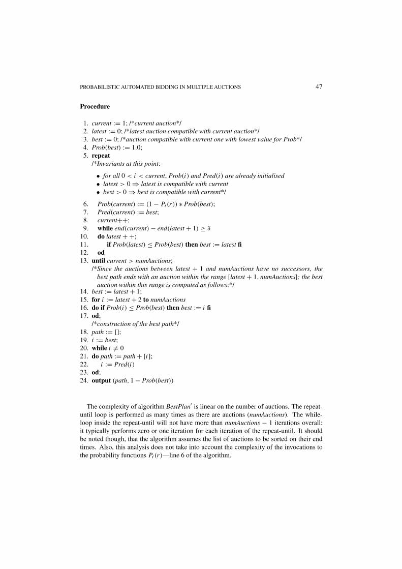
Procedure

1. current := 1; /*current auction*/2. latest := 0; /*latest auction compatible with current auction*/3. best := 0; /*auction compatible with current one with lowest value for Prob*/4. Prob(best) := 1.0;5. repeat

/*Invariants at this point:

• for all 0 < i < current, Prob(i) and Pred(i) are already initialised• latest > 0 ⇒ latest is compatible with current• best > 0 ⇒ best is compatible with current*/

6. Prob(current) := (1 − Pi(r)) ∗ Prob(best);7. Pred(current) := best;8. current++;9. while end(current) − end(latest + 1) ≥ δ

10. do latest + +;11. if Prob(latest) ≤ Prob(best) then best := latest fi12. od13. until current > numAuctions;

/*Since the auctions between latest + 1 and numAuctions have no successors, thebest path ends with an auction within the range [latest + 1, numAuctions]; the bestauction within this range is computed as follows:*/

14. best := latest + 1;15. for i := latest + 2 to numAuctions16. do if Prob(i) ≤ Prob(best) then best := i fi17. od;

/*construction of the best path*/18. path := [];19. i := best;20. while i �= 021. do path := path + [i];22. i := Pred(i)

23. od;24. output (path, 1 − Prob(best))

The complexity of algorithm BestPlan′ is linear on the number of auctions. The repeat-until loop is performed as many times as there are auctions (numAuctions). The while-loop inside the repeat-until will not have more than numAuctions − 1 iterations overall:it typically performs zero or one iteration for each iteration of the repeat-until. It shouldbe noted though, that the algorithm assumes the list of auctions to be sorted on their endtimes. Also, this analysis does not take into account the complexity of the invocations tothe probability functions Pi(r)—line 6 of the algorithm.

48 DUMAS ET AL.

Notes

1. In a proxy bid [7], the user bids at the current quote, and authorises the auction house to bid on its behalf upto a given amount. Subsequently, every time that a new bid is placed, the auction house counter-bids on theuser’s behalf up to the authorised amount.

2. Under the assumption of perfect rationality, it is an optimal strategy for a bidder in an “isolated” FPSB auctionto bid the maximum amount that (s)he intends to pay minus a “bid shaving” factor which depends on thenumber of bidders in the auction [Sandholm, 14]. Similar “bid shaving” results exist for sequential auctions[Weber, 19].

3. Note that in this case the bidding plan does not need to be computed entirely, but only the first auction in theplan needs to be determined, since a revision will occur immediately after this auction (if it is lost).

4. We also run the same experiment with creationTime = 0.4 and 0.6 and obtained similar results. In fact, thecreation time is only there to ensure that there are sufficient bid histories before the probabilistic bidders enterthe market.

References

[1] Anthony, P. and N. Jennings. (2003). “Developing a Bidding Agent for Multiple Heterogeneous Auctions.”ACM Transactions on Internet Technology 3(3), 185–217.

[2] Bansal, V. and R. Garg. (2000). “On Simultaneous Online Auctions with Partial Substitutes.” Technical Re-port, IBM India Research Lab. http://www.research.ibm.com/iac/papers/ri00022.pdf,accessed on 10 November 2001.

[3] Byde, A. (2001). “An Optimal Dynamic Programming Model for Algorithm Design in Simultane-ous Auctions.” Technical Report HPL-2001-67, HP Labs, Bristol, UK. http://www.hpl.hp.com/techreports/2001/HPL-2001-67.html

[4] Cormen, T., C. Leiserson, and R. Rivest. (1990). Introduction to Algorithms. MIT Press.[5] D’Agostino, R., A. Belanger, and R. D’Agostino Jr. (1990). “A Suggestion for Powerful and Informative

Tests of Normality.” The American Statistician 44(4), 316–321.[6] Dumas, M., G. Governatori, A. ter Hofstede, and N. Russell. (2002). “An Architecture for Assembling

Agents that Participate in Alternative Auctions.” In Proc. of the Workshop on Research Issues in DataEngineering (RIDE), San Jose, CA, USA, pp. 75–83.

[7] eBay. “Proxy bidding.” http://www.ebay.com/help/buyerguide/bidding-prxy.html,accessed 10 November 2001.

[8] Garcia, P., E. Gimenez, L. Godo, and J. Rodriguez-Aguilar. (1998). “Possibilistic-Based Design of BiddingStrategies in Electronic Auctions.” In Proc. of the 13th European Conference on Artificial Intelligence(ECAI), Brighton, UK, pp. 575–579.

[9] Greenwald, A. and P. Stone. (2001). “Autonomous Bidding Agents in the Trading Agent Competition.”IEEE Internet Computing 5(2), 52–60.

[10] Lucking-Reiley, D. (2000). “Auctions on the Internet: What’s Being Auctioned, and How?” Journal ofIndustrial Economics 48(3), 227–252.

[11] Martello, S. and P. Toth. (2001). Knapsack Problems: Algorithms and Computer Implementations. NewYork: Wiley.

[12] Preist, C., A. Byde, and C. Bartolini. (2001). “Economic Dynamics of Agents in Multiple Auctions.” InProc. of the 5th International Conference on Autonomous Agents, Montreal, Canada, pp. 545–551.

[13] Roth, A. and A. Ockenfels. (2002). “Last-Minute Bidding and the Rules for Ending Second-Price Auctions:Evidence from eBay and Amazon Auctions on the Internet.” American Economic Review 92(4), 1093–1103.

[14] Sandholm, T. (1999). “Distributed Rational Decision Making.” In [Weiss, 20], pp. 201–258.[15] Schapire, R., P. Stone, D. McAllester, M. Littman, and J. Csirik. (2002). “Modeling Auction Price Uncer-

tainty Using Boosting-Based Conditional Density Estimation.” In Proc. of the 19th International Confer-ence on Machine Learning, Sydney, Australia, pp. 546–553.


[16] Shehory, O. (2002). “Optimal Bidding in Multiple Concurrent Auctions.” International Journal of Cooper-ative Information Systems 11(3–4), 315–327.

[17] Tewari, G. and P. Maes. (2001). “Generalized Platform for the Specification, Valuation, and Brokering ofHeterogeneous Resources in Electronic Markets.” In J. Ye and Y. Ye (eds.), E-Commerce Agents, LectureNotes in Computer Science, Vol. 2033. Berlin: Springer.

[18] Thisted, R. (1988). Elements of Statistical Computing. New York: Chapman & Hall.[19] Weber, R. (1983). “Multiple-Object Auctions.” In R. Englebrecht-Wiggins, M. Shubick, and R. Stark (eds.),

Auctions, Bidding, and Contracting: Uses and Theory. New York University Press, pp. 165–191.[20] Weiss, G. (ed.). (1999). Multiagent Systems: A Modern Introduction to Distributed Artificial Intelligence.

Cambridge, MA: MIT Press.[21] Wellman, M., A. Greenwald, P. Stone, and P. Wurman. (2002). “The 2002 Trading Agent Competition.” In

Proc. of the 14th Innovative Applications of Artificial Intelligence Conference, Edmonton, Canada, pp. 935–942.

[22] Zeithammer, R. (2003). “Forward-Looking Bidders in Sequential Auctions.” Ph.D. Thesis, MIT SloanSchool of Business.

[23] Zhu, W. and P. Wurman. (2002). “Structural Leverage and Fictitious Play in Sequential Auctions.” In Proc.of the American Artificial Intelligence Conference (AAAI), Edmonton, Canada, pp. 385–390.

probabilistic automated bidding in multiple auctions

Documents