probabilistic fire simulator fusarium vtt · pdf filethe intelligence of intelligent...
TRANSCRIPT

VTT PU
BLICATIO
NS 503
Probabilistic Fire Simulator. Theory and...
Simo H
ostikka, Olavi K
eski-Rahkonen & Tim
o Korhonen
Tätä julkaisua myy Denna publikation säljs av This publication is available from
VTT TIETOPALVELU VTT INFORMATIONSTJÄNST VTT INFORMATION SERVICEPL 2000 PB 2000 P.O.Box 200002044 VTT 02044 VTT FIN�02044 VTT, Finland
Puh. (09) 456 4404 Tel. (09) 456 4404 Phone internat. +358 9 456 4404Faksi (09) 456 4374 Fax (09) 456 4374 Fax +358 9 456 4374
ISBN 951–38–6235–6 (soft back ed.) ISBN 951–38–6236–4 (URL: http://www.vtt.fi/inf/pdf/)ISSN 1235–0621 (soft back ed.) ISSN 1455–0849 (URL: http://www.vtt.fi/inf/pdf/)
ESPOO 2003ESPOO 2003ESPOO 2003ESPOO 2003ESPOO 2003 VTT PUBLICATIONS 503
Simo Hostikka, Olavi Keski-Rahkonen &Timo Korhonen
Probabilistic Fire Simulator
Theory and User's Manual for Version 1.2
VTT PUBLICATIONS
485 Kärnä, Tuomo, Hakola, Ilkka, Juntunen, Juha & Järvinen, Erkki. Savupiipun impakti-vaimennin. 2003. 61 s. + liitt. 20 s.
486 Palmberg, Christopher. Successful innovation. The determinants of commercialisation andbreak-even times of innovations. 2002. 74 p. + app. 8 p.
487 Pekkarinen, Anja. The serine proteinases of Fusarium grown on cereal proteins and in barleygrain and their inhibition by barley proteins. 2003. 90 p. + app. 75 p.
488 Aro, Nina. Characterization of novel transcription factors ACEI and ACEII involved inregulation of cellulase and xylanase genes in Trichoderma reesei. 2003. 83 p. + app. 25 p.
489 Arhippainen, Leena. Use and integration of third-party components in software develop-ment. 2003. 68 p. + app. 16 p.
490 Vaskivuo, Teemu. Software architecture for decentralised distribution services in spontane-ous networks. 2003. 99 p.
491 Mannersalo, Petteri. Gaussian and multifractal processes in teletraffic theory. 2003. 44 p.+ app. 109 p.
492 Himanen, Mervi. The Intelligence of Intelligent Buildings. The Feasibility of the IntelligentBuilding Consept in Office Buildings. 2003. 497 p.
493 Rantamäki, Karin. Particle-in-Cell Simulations of the Near-Field of a Lower Hybrid Grill.2003. 74 p. + app. 61 p.
494 Heiniö, Raija-Liisa. Influence of processing on the flavour formation of oat and rye. 2003.72 p. + app. 48 p.
495 Räsänen, Erkki. Modelling ion exchange and flow in pulp suspensions. 2003. 62 p. + app.110 p.
496 Nuutinen, Maaria, Reiman, Teemu & Oedewald, Pia. Osaamisen hallinta ydinvoima-laitoksessa operaattoreiden sukupolvenvaihdostilanteessa. 2003. 82 s.
497 Kolari, Sirpa. Ilmanvaihtojärjestelmien puhdistuksen vaikutus toimistorakennusten sisäil-man laatuun ja työntekijöiden työoloihin. 2003. 62 s. + liitt. 43 s.
498 Tammi, Kari. Active vibration control of rotor in desktop test environment. 2003. 82 p.499 Kololuoma, Terho. Preparation of multifunctional coating materials and their applications.
62 p. + app. 33 p.500 Karppinen, Sirpa. Dietary fibre components of rye bran and their fermentation in vitro.
96 p. + app. 52 p.501 Marjamäki, Heikki. Siirtymäperusteisen elementtimenetelmäohjelmiston suunnittelu ja
ohjelmointi. 2003. 102 s. + liitt. 2 s.503 Simo Hostikka, Olavi Keski-Rahkonen & Timo Korhonen. Probabilistic Fire Simulator.
Theory and User's Manual for Version 1.2. 2003. 72 p. + app. 1 p.


VTT PUBLICATIONS 503
Probabilistic Fire SimulatorTheory and User's Manual for Version 1.2
Simo Hostikka, Olavi Keski-Rahkonen & Timo KorhonenVTT Building and Transport

ISBN 951�38�6235�6 (soft back ed.)ISSN 1235�0621 (soft back ed.)
ISBN 951�38�6236�4 (URL: http://www.vtt.fi/inf/pdf/)ISSN 1455�0849 (URL: http://www.vtt.fi/inf/pdf/)
Copyright © VTT Technical Research Centre of Finland 2003
JULKAISIJA � UTGIVARE � PUBLISHER
VTT, Vuorimiehentie 5, PL 2000, 02044 VTTpuh. vaihde (09) 4561, faksi (09) 456 4374
VTT, Bergsmansvägen 5, PB 2000, 02044 VTTtel. växel (09) 4561, fax (09) 456 4374
VTT Technical Research Centre of Finland, Vuorimiehentie 5, P.O.Box 2000, FIN�02044 VTT, Finlandphone internat. + 358 9 4561, fax + 358 9 456 4374
VTT Rakennus- ja yhdyskuntatekniikka, Kivimiehentie 4, PL 1803, 02044 VTTpuh. vaihde (09) 4561, faksi (09) 456 4815
VTT Bygg och transport, Stenkarlsvägen 4, PB 1803, 02044 VTTtel. växel (09) 4561, fax (09) 456 4815
VTT Building and Transport, Kivimiehentie 4, P.O.Box 1803, FIN�02044 VTT, Finlandphone internat. + 358 9 4561, fax + 358 9 456 4815
Technical editing Marja Kettunen
Otamedia Oy, Espoo 2003

3
Hostikka, Simo, Keski-Rahkonen, Olavi & Korhonen, Timo. Probabilistic Fire Simulator. Theoryand User´s Manual for Version 1.2. Espoo 2003. VTT Publications 503. 72p. + app. 1 p.
Keywords fire prevention, fire safety, simulation, simulators, user manual, risk analysis,computation, calculations, models, estimation
AbstractRisk analysis tool is developed for computation of the distributions of fire modeloutput variables. The tool, called Probabilistic Fire Simulator, combines MonteCarlo simulation and CFAST two-zone fire model. This document describes thephysical models and contains a detailed user's manual. In the applications, thetool is used to estimate the failure probability of redundant cables in a cabletunnel fire, and the failure and smoke filling probabilities of electronics roomduring a fire of an electronics cabinet. Sensitivity of the output variables to theinput variables is calculated in terms of the rank order correlations. Various stepsof the simulation process, i.e. data collection, generation of the inputdistributions, modelling assumptions, definition of the output variables and theactual simulation, are described.

4
PrefaceThis study was carried out as a part of the Fire Safety Research project (FISRE)which is one of the projects in the Finish Research Programme on the NuclearPower Plant Safety (FINNUS).
The study has been financed by the Finnish Centre for Radiation and NuclearSafety, the Ministry of Trade and Industry, Fortum Engineering Ltd andTeollisuuden Voima Oy.
The theory and user's manuals are here given for the Version 1.2 of theProbabilistic Fire Simulator -software. These are the first published versions ofthe manuals.

5
Contents
Abstract................................................................................................................. 3
Preface .................................................................................................................. 4
THEORY AND APPLICATIONS ....................................................................... 7
List of symbols...................................................................................................... 8
1. Introduction..................................................................................................... 91.1 General background............................................................................... 91.2 Present task.......................................................................................... 11
2. Monte Carlo Simulation ............................................................................... 13
3. Fire modelling............................................................................................... 153.1 Smoke spreading ................................................................................. 153.2 Cable heating....................................................................................... 153.3 RHR in room fires ............................................................................... 19
4. Results and discussion .................................................................................. 224.1 Cable tunnel fire scenario.................................................................... 224.2 Electronics room fire scenario............................................................. 29
5. Summary....................................................................................................... 34
USER'S MANUAL............................................................................................. 36
6. Software and hardware requirements ........................................................... 37
7. Definitions .................................................................................................... 38
8. Using Probabilistic Fire Simulator ............................................................... 408.1 General ................................................................................................ 408.2 Fire model user interface ..................................................................... 40
8.2.1 Set parameters ......................................................................... 428.2.2 Define geometry...................................................................... 428.2.3 Define materials ...................................................................... 438.2.4 Define RHR curve................................................................... 44
6
8.2.5 Define fire source properties................................................... 458.2.6 Define target............................................................................ 458.2.7 Define sprinklers and detectors ............................................... 478.2.8 Run simulation ........................................................................ 488.2.9 Read results ............................................................................. 48
8.3 Monte-Carlo simulation....................................................................... 498.3.1 Start @RISK ........................................................................... 498.3.2 Open PFS workbook ............................................................... 498.3.3 Definition section .................................................................... 498.3.4 Define random variables ......................................................... 518.3.5 Define output variables ........................................................... 528.3.6 Set simulation parameters ....................................................... 528.3.7 Run simulation ........................................................................ 538.3.8 Read results ............................................................................. 53
9. Input variables and parameters ..................................................................... 549.1 Main..................................................................................................... 549.2 Control................................................................................................. 549.3 Random Variables ............................................................................... 579.4 Zone Model Input ................................................................................ 589.5 Distributions ........................................................................................ 639.6 Thermal Database................................................................................ 63
10. Modifying PFS.............................................................................................. 6510.1 PFS Workbook .................................................................................... 6510.2 Visual Basic functions and subroutines............................................... 6610.3 Fortran functions ................................................................................. 67
References........................................................................................................... 68
AppendicesAppendix A: Computation of the roots βi for the cable heat transfer equation

7
THEORY AND APPLICATIONS

8
List of symbols
Afuel Area of the fuel surface inside the electronics cabinetAe Area of the cabinet exhaust openingAi Area of the cabinet inflow openingBi Biot numberFo Fourier numberFi Probability distribution function of variable ifi Probability density function of variable igA Limit state functionHv Height between the cabinet openingsh Linearized heat transfer cofficientk Conductivityn Number of random variablesPA Probability of event AQ Fire loadQ� Rate of heat release (RHR)
fuelQ ′′� Rate of heat release per fuel areaRcable Cable outer radiusRcore Cable core radiusr Radial positionX, x Vector of random variablesx Random variableT Temperaturet Timetg RHR growth timeGreek lettersα Thermal diffusivityχ Combustion efficiency∆Hc Heat of combustionφX Joint probability density functionτd Decay time constant of heat release rate

9
1. Introduction1.1 General background
A quantitative assessment of the various effects of fire within buildings andother constructions using computational tools is a challenging mathematicalproblem. Buildings can be considered as systems, which respond to an externalevent, like fire, in a complicated way. Although the actual nature of the responsemay be deterministic or stochastic, the former is usually assumed forengineering applications. Time averages, or sample averages, which can bemodelled in a deterministic way, yield values of design variables needed fordimensioning. Besides the building itself, there are different objects within thebuilding that are influenced by the fire, for example people and mechanicaldevices. The factors influencing the response of these objects are againdeterministic, probabilistic, or mixtures of both.
Presuming we had an accurate mathematical model of fire, solvable by anumerical computer code, we could, in principle, predict values of all the factorsas a function of time, and let them influence the target selected for responsestudy. Estimating uncertainty in such a system would be rather straightforward,because for a given scenario, calculating the consequences of fire ismathematically a fairly well-posed problem. The applied numericalapproximations usually filter out the spatial and temporal fluctuations, caused bythe stochastic nature of some phenomena. Therefore, the major uncertainty in thefinal results is caused by some, rather narrow uncertainty margins of the physicalinput variables. Both the estimation of these distributions and propagation of theimplied uncertainty through the system could be calculated using standardtechniques. Our experience on such systems suggests that these errors remainwithin a factor of two in fire scenarios needed for building design. Cases wheredeterministic modelling of the response is difficult or missing, are naturallyexceptions.
A fire scenario is here defined as a layout of the fire scene, where a set of fireand response models is able to give deterministic values for target parameters,once the numerical inputs are given. Analogous to statistical physics, a subset ofthe scenario, where each of the input variables has a definite value, is called stateone. This state is represented by a point in a hyperspace spanned by the input

10
vectors. Similarly, the target is also not a unique state, but a collection of stateswithin the scenario. To produce values needed for practical work, we have tosum up over a large number of well-defined initial and final states, systemaverages in terms of statistical mechanics.
Typically, the variability of system or target parameters, like the amount of fireload, is much bigger than the variability of physical input variables, like heatconductivity of a material. For this reason, they cannot be filtered out oraveraged by any formal means. Usually, the system variables must be introducedin calculations through statistical distributions. Although our fire and responsemodel is quasi-deterministic, the prediction of target response distributionsrequires combination of deterministic and stochastic calculation methods. Afurther problem, not encountered here yet, is the lack of data: there might bevariables for which we do not have data either because no one has studied it orbecause it might be difficult to obtain. During the formulation of the problem,one must be aware of these variables because they might affect the way theuncertainty propagates through the system.
There is a lot of mathematical literature available on these problems outside firescience. Earlier works [see reviews by Hannus 1973 and Spiegel 1980]concentrated much on deterministic systems, where input variables weregoverned by well defined classical, like normal or lognormal distributions. Vastincrease of computing power during the recent years has created interest tomodel large complicated systems like nuclear power plants, where theunavailability of data inevitably plays an important role. Questions of aleatoryand epistemic treatment arise. A good introduction to the recent developments isgiven by Helton and Burmaster [1996] in an editorial to a special issue inReliability Engineering and System Safety. Philosophical and practical aspectsof the problem are discussed in special articles in the same issue [Ferson &Ginzburg 1996, Parry 1996, Paté-Cornell 1996, Theofanous 1996, Winkler1996]. Textbook on the subject [Vose 1996] gives detailed guidance, and theapplication examples of Hofer et al. [2001, 2002] present some possible results.
11
1.2 Present task
Traditionally, the deterministic fire models have been used to estimate, what arethe typical consequences of the fire, at the given values for the input parameters.The possible uncertainty or distribution of the input variables has been taken intoaccount by manually varying the inputs, or carrying out classical error analysisin analytical or other formal way. The goal of this study is to develop a generaltool for the probabilistic estimation of fire consequences by combiningdeterministic numerical simulation with tools of stochastic nature. Similar toolshave been available for some time for calculations of severe accidents in NPPs,like that of Hofer et al. [2002]. For fire analyses, a landmark of probabilisticapproach was the evaluation of partial safety factors in ref. [CIB W14, 1986]. Itwas a classical example of error propagation, where good deterministic modelswere available for the physics. More advanced methods have been reviewedrecently by Magnusson [1997], but no single method has been established yet.One of the recent applications is again on nuclear sector [Haider et al. 2002]. Forpractical reasons, the present work is limited to those scenarios, which webelieve can be modelled deterministically, and thus remain safely on theepistemic realm.
A specific task is the prediction of the failure probabilities of specified items infires. A risk analysis model is developed using the well-known technique ofMonte Carlo simulations. A commercial Monte Carlo simulation software@RISK is used for the random sampling and data processing. A two-zone modelCFAST [Peacock et al. 1993] is used to model smoke spreading and gastemperature during the fire. The risk analysis model and the physical models arecombined in a spreadsheet computing environment. The tool, called ProbabilisticFire Simulator (PFS), is intended to be fully general and applicable to any firescenario amenable to deterministic numerical simulation. The main outcome ofthe new tool is the automatic generation of the distributions of the selected resultvariables, for example component failure time. The sensitivity of the outputvariables to the input variables can be calculated in terms of the rank ordercorrelations. Sensitivity calculations are performed using plausible input datadistributions to find out the most important parameters. The simulation processconsists of the following steps: data collection, generation of the inputdistributions, modelling and assumptions, definition of the output variables andthe actual Monte Carlo simulation.

12
Two example cases are here studied: a fire in a nuclear power plant cable tunneland a fire in an electronics room. The cable tunnel fire was studiedexperimentally by Mangs & Keski-Rahkonen [1997] and theoretically by Keski-Rahkonen & Hostikka [1999]. These studies showed that CFAST two-zonemodel can be used to predict the thermal environment of a cable tunnel fire, atleast in its early stages. Here, the effects of the tunnel geometry and fire sourceproperties are studied by sampling the input variables randomly from thedistributions. The input distributions are based on the statistics collected fromthe power plant.
The electronics room fire was previously studied by Eerikäinen & Huhtanen[1991]. They used computational fluid dynamics to predict the thermalenvironment inside the room, when one electronics cabinet is burning. The samescenario is studied here using the two-zone model. The fire source is selectedrandomly based on the collected distribution of different cabinet types.

13
2. Monte Carlo SimulationThe question set by the probabilistic safety assessment process is usually: �Whatis the probability that a certain component or system is lost during a fire?� Thisprobability is a function of all possible factors that may affect on thedevelopment of the fire and the systems reaction. This question has not beendealt with exactly for fire in this form, but similar systems on the other fieldshave been studied extensively [Spiegel 1980, Hannus 1973, Vose 1996]. Herewe adapt this general theory for our specific fire problem.
Let us denote the group of affecting variables by vector ( )TnXXX ...21=X
and the corresponding density functions fi and distribution functions Fi. Theoccurrence of the target event A is indicated by a limit state function gA(t,x),which is a non-increasing function of time t and vector x containing the valuesof the random variables. As an example, we define a limit state condition for aloss of component using function gA(t,x):
ttgttg
A
A
at timelost not iscomponent if ,0),( at timelost iscomponent if ,0),(
>≤
xx (1)
The development of fire and the response of the components under considerationare assumed to fully deterministic processes where similar initial and boundaryconditions always lead to the same final condition. With this assumption theprobability of event A can now be calculated by integral
{ }�� �
≤
=0),(
)()(xx
xtg
ixA
A
dxtP φ�(2)
where φx is the joint density function of variables X. Generally variables X aredependent, and ∏ =
≠ n
i iix xf1
)()(xφ .
In this work, the probability PA is calculated using Monte Carlo simulationswhere input variables are sampled randomly from the distributions Fi. If gA(t,x)is expensive to evaluate, stratified sampling technique must be used. In LatinHypercube sampling (LHS) the n-dimensional parameter space is divided into Nn
cells [McKay et al. 1979]. Each random variable is sampled in fully stratified

14
way and then these samples are attached randomly to produce N samples from ndimensional space. The advantage of this approach is that the random samplesare generated from all the ranges of possible values, thus giving insight into thetails of the probability distributions. A procedure for obtaining a LatinHypercube sample for multiple, spatially correlated variables is given by Stein[1987]. He showed that LHS will decrease the variance of the resulting integralrelative to the simple random sampling whenever the sample size N is largerthan the number of variables n. However, the amount of reduction increases withthe degree of additivity in the random quantities on which the function beingsimulated depends. In fire simulations, the simulation result may often be astrongly nonlinear function of the input variables. For this reason, we can notexpect that LHS would drastically decrease the variances of the probabilityintegrals. Problems related to LHS with small sample sizes are discussed byHofer [1999] as well as by Pebesma & Heuvelink [1999].
The sensitivity of the output y to the different input variables x is studied bycalculating the Spearman�s rank-order correlation coefficients (RCC). A value�s�rank� is determined by its position within the min-max range of possible valuesfor the variable. RCC is then calculated as
)1(6
1RCC 2
2
−−= �
nnd (3)
where d is the difference between ranks of corresponding x and y, and n is thenumber of data pairs. RCC is independent of the distribution of the initialvariable. The significance of the RCC values should be studied with the methodsof statistical testing. In case of small data sets, the actual values of RCC shouldbe interpreted with caution due to the possible spurious correlations inside theinput data [Hofer 1999].

15
3. Fire modelling3.1 Smoke spreading
The transport of heat and smoke is simulated using a multi-room two-zonemodel CFAST [Peacock et al. 1993]. It assumes two uniform layers, hot andcold, in each room of the building and solves the heat and mass balanceequations for each room. PFS worksheet is used to generate the input data forCFAST. The user may combine any experimental information or functions to thefire model input. The most important source term in the simulation is the rate ofheat release (RHR). The RHR can be defined using analytical curves, like t2-curve [Heskestad & Delichatsios 1977, NFPA 1985], or specific experimentalcurves.
Typical results of the fire simulation are gas temperatures, smoke layer positionand temperature of some solid object like cable. Usually, the actual targetfunction is the time when some event takes place. Some examples of the targetfunctions are smoke filling time, flash over time and component failure time. Inthis work, the most important target function is the cable failure time. Thesolution of the cable heating is explained in the following section.
3.2 Cable heating
The heat transfer from the gas space to a cable is studied separately from the firesimulations and flame spread calculations. The calculation is based on thelinearized model presented by Keski-Rahkonen et al. [1999]. Their modelassumes an axially symmetric heat conduction inside a cylinder, with a radiusRcable and varying ambient temperature T∞(t). Thermal properties of the cable,radius of the cable and the heat transfer coefficient must be considered randomvariables, as they are usually not known accuratelly.
If the metal core is omitted and homogenous insulation material is assumed, thecable insulator temperature T(r,t), which is a function of radial position r andtime t, can be written in an analytical form

16
�=
Φ+
=β
βββββα N
iNi
cableicableii
icablei
cableN t
RJRJbrJR
RtrT
1 10
02
2 )()(Bi)(
)(Bi2),((4)
where α2 is thermal diffusivity of the cable insulator material, Nβ is the numberof terms in the series and iβ are the roots of equation
0Bi
)()( 10 =− cableicablei
cableiRJRRJ βββ , i = 1, 2, 3, �
(5)
where J0 and J1 are Bessel functions. Φi is the convolution sum of the gastemperature and exponential decay terms, as described later. Bi is the biotnumber
khRcable /Bi = (6)
where h is the linearized heat transfer coefficient at the cable surface and k is theconductivity of the insulator.
Equation (4) is relatively easy to implement, but the actual calculation is timeconsuming because the solution involves the roots of a non-linear equation.These roots must be recalculated to a high accuracy at each time step. For fastcalculation the roots were precalculated and tabulated. The calculation methodof roots βi is explained in Appendix A. Simple and fast interpolation scheme wasthen used to find the approximation for the roots. The accuracy and calculationtime can be controlled by selecting the number of roots (i.e. the number of termsin the solution series) to be used. Another time consuming part of the calculationis the convolution sum
�=
−−∆−����
�� +=Φ
N
j
tttijijijNi
jNiji eeBACt1
)(22
22)( βαβα (7)
where 1−−=∆ jjj ttt and

17
( )( )
( )222
1,2
2,
,2
21,
1
1
1
ijij
jijjij
jijjij
tC
TtTB
TtTA
βα
βα
βα
∆=
+∆−=
−∆+=
−∞∞
∞−∞ (8)
where T∞,j is the ambient temperature at time tj. If we assume that the roots βi
change slowly, and change the order of summation in (4), it can be re-arrangedto form
( )���
�+
���
�+Φ=
∆−∆−
=
−=
∆−
�
�
NiNi
Ni
ttiNiNiN
N
ii
Ni
N
ii
t
cableN
eeBACS
tSeR
trT
22
2
1
11
22 )(2),(
αβαβ
αβ
β
βα (9)
where Si is defined as
)(Bi)()(Bi
10
0
cableicableii
icableii RJRJb
rJRSβββ
ββ+
=(10)
In Equation (9), the terms of the first sum inside the brackets are the termscorresponding to the previous time steps in a recursive manner. Cabletemperature at time step tN now depends on two parts: exponentially decayingmemory of the cable temperature at the previous time step tN-1 and the morerecent effect of the gas temperature. Long convolution sums are not needed.Combined to the precalculated root tables this method was noticed to be fastenough to be applicable in Monte-Carlo simulations.
The accuracy of the analytical solutions was studied by comparing them to theresults calculated with a numerical model applying finite element method(FEM). Figures 1 and 2 show the relative errors of the cable surface temperatureas a function of the Fourier number Fo, in various cable configurations. TheFourier number Fo represents the dimensionless time for transient conduction[Carlslaw & Jaeger 1959]
18
2FocableR
tα= (11)
The thermal boundary condition on the cable surface was a convective andradiative heat flux from a constant gas temperature 200°C. For all studied casesthe magnitude of the error is acceptable, taking into account the generaluncertainties related to the fire modelling.
R cable = 5 mm, T gas = 200 °C
-10
-5
0
5
10
15
0.01 0.1 1 10Fo
100
× ( θ
A- θ
FEM
)/θF
EM
(%)
0.010.250.50.75
R core /R cable
Figure 1. Relative errors of the cable surface temperature predictions of theanalytical model for a 5 mm thick cable. Four curves correspond to differentrelative sizes of the metal core. For a fixed thermal properties and radius, thehorizontal axis represents time.
The FEM models contained both the PVC insulation layer and the metal core ofthe cable. The analytical model in turn neglects the effect of the metal core, andassumes a homogenous cylindrical insulation material. In case of 10 mm thickcable (Rcable = 5 mm), shown in Figure 1, the errors are smallest when the metalcore radius Rcore is small compared to Rcable. For a cable with radius 30 mm,which could be a thick power cable, the results are somewhat inconsistent withthe thinner case. The best accuracy is achieved with the largest Rcore/Rcable -ratio,as shown in Figure 2. This inconsistency is caused by the limited number ofterms in the series representation of the analytical solution.

19
R cable = 30 mm, T gas = 200 °C
-10
-8
-6
-4
-2
0
2
0.01 0.1 1 10Fo
100
× ( θ
A- θ
FEM
)/θF
EM
(%) 0.01
0.250.50.75
R core /R cable
Figure 2. Relative errors of the cable surface temperature predictions of theanalytical model for a 30 mm thick cable. See the explanation in the caption ofFigure 1.
3.3 RHR in room fires
For a fire scenario in a compartment, rate of heat release (RHR) cannot becalculated using ab initio methods except for some very simple cases. If the fireload is small and fire size tiny, in relation to compartment size, fire remainslocal. In this simple case some theoretical methods can be applied to simplefuels, or direct calorimetric experiments for more complicated objects likeelectronic equipment or household utilities.
In compartments where fire size is comparable with room dimensions, or fire islikely to become oxygen limited, simple engineering methods can be derivedfrom experimental correlations and boundary conditions. For fire growth t2-typetemporal behaviour was observed experimentally [Heskestad & Delichatsios1977], which has already achieved a standard status [NFPA 1985]. The model isalso adopted to ISO/PDTR 13387 document redefining growth factor as growthtime tg, slightly differently from NFPA 204M to fit in the metric unit of time.After flashover fire becomes oxygen limited [Drysdale 1985], and thus RHR

20
remains roughly constant. Combining these observations to exponential decay offire with decay time constant τd, we obtain a relationship, which combinesmaximum RHR to fire load Q and size of openings of the compartment, as wellas to characteristic duration of full burning td [Keski-Rahkonen 1993]. Takingthe integral of RHR over the whole burning time, a relation to total fire load Q isobtained
cHmQdttQ ∆==�∞
χχ0
)(� (12)
where )(tQ� is the RHR, χ is efficiency of burning, m total mass of fire load andcH∆ heat of combustion of the material. Carrying out the integrations in closed
form a polynomic relation between times is obtained
Qtttt
ddg
χτ =+− )()( 13221
(13)
where t1 is the time when maximum RHR is reached.
In a room fire scenarios, the growth time tg and the decay time constant τd arefound to be correlated and logarithmically normally distributed [Linkova &Keski-Rahkonen 2002, Linkova et al. 2003]. For unconstrained scenario
ngd tc=τ (14)
where c ≈ 4.48 and n ≈ 0.69, when times as expressed in seconds. Thecumulative distribution functions of τd and tg are
��
���
>−+<−−
=−ββ
021
021
0 ),1(),1(
)(xxzerfxxzerf
xxF (15)
where

21
[ ] ∞≤≤≤>>−= xxxxz 00 0,0,0
2/)(ln βα
αβ (16)
For cumulative estimates, median ranks were used throughout (McCormick1981). Fitting by inspection, the following rough estimates for the parameterswere obtained; for τd : x0 = 3 s, α = 1.3, and β = 221s, and for tg : x0 = 3 s, α =1.15, and β = 270 s.
Fire loads are also roughly logarithmically normally distributed althoughWeibull and Gumbel distributions could be fitted equally well [Korpela &Keski-Rahkonen 2000].
For special scenarios RHR data may be tailored from local constraints, whichmay differ radically from these general trends.

22
4. Results and discussion4.1 Cable tunnel fire scenario
A fire in the cable tunnel of a nuclear power plant is simulated to find out thefailure probability of cables located in the same tunnel with the fire. The fireignites in a cable tray and the fire gases heat up a redundant cable, located on theopposite side of the same tunnel. An effect of possible screen that divides thetunnel between the source and target is studied. The distribution of the heatdetector activation times is also calculated. A plan view of the physical geometryand the corresponding CFAST model are outlined in Figure 3. A vertical cut ofthe tunnel is shown in Figure 4. The tunnel is divided in five virtual rooms toallow horizontal variations in layer properties. The fire source is located inROOM 1 and the target cable in ROOM 3, just on the opposite side of thescreen. The length of the screen does not cover the whole tunnel, and therefore itis possible that smoke flows around the screen to the target. It is also possible,that smoke flows below the screen. In the end of the tunnel is a door to theambient. The rate of heat release (RHR) from the fire source is modelled usingan analytical t2-type curve
��
��
�
��
��
�
��
��
�
⋅=
2
max 1000 ,min)(gttQtQ �� [kW] (17)
where t is time, tg is the RHR growth time and maxQ� is the maximum RHR,which depends on the tunnel size. tg is treated as a normally distributed randomvariable with mean of 1000 s and standard deviation of 300 s. The lognormaldistribution, suggested in Section 3.3, is not used because the data was notavailable at the time of the simulations.

23
y
x
ROOM 1 ROOM 2
ROOM 3 ROOM 4
ROOM 5
DO
OR
Tunnel length L
Tunn
el w
idth
W
screen
A
A�
Room 1 length Room 2 length
Figure 3. A plan view of the cable tunnel model.
z
y
Tunn
el h
eigh
t H
sourcez targ
etD2 D1
z scre
en
A - A�
scre
entarget
Tunnel width W
Figure 4. A vertical cut A-A' of the cable tunnel model. D1 and D2 denote heatdetectors 1 and 2, respectively.
Two different versions of the scenario are studied. First, the screen is assumed toexist, with the height of the lower edge being a random variable between zeroand 50 % of the tunnel height. In the second scenario, the screen is removed bysetting the lower edge very close to the ceiling, retaining the virtual roomstructure of the model. The dimensions of the tunnel and the cable tray locationsare taken from the measured distributions of the power plant. About 50 tunnelcross sections have been studied to generate the distributions. The distribution ofthe cable diameter is based on the measurements in seven tunnel cross sections,containing 815 cables. A complete list of the random variables is given in Table1. While most of the variables are true physical properties and dimensions, thelengths of the virtual rooms are purely associated to the numerical model. They
24
are treated as random variables to examine the sensitivity of the model. It isdesirable that these variables are less important than the true physical variables.
Table 1. A list of random variables used in the cable tunnel fire scenario."Measured"-text in the distribution column means that measured histogramsfrom the true power plant are used as sampling distributions.
Variable Distribution Mean Std.dev Min Max Units
RHR growth time tg Normal 1000 300 0 3000 sSource height zsource/H Uniform 0 0.7Ambient temperature Normal 20 3.0 °CTunnel height H Measured mTunnel width Wtunnel Measured mRoom 1 length Uniform 2 5 mRoom 2 length Uniform 5 10 mTunnel length L Uniform 30 100 mDoor height zdoor/H Uniform 0.1 1.0Door width Wdoor /Wtunnel Uniform 0.01 1.0Screen edge height zscreen/H Uniform 0 / 0.95 0.5 / 1.0Dimensionless cable height ztarget/H MeasuredCable radius Measured mmCritical cable temperature Normal 200 20 °CCable conductivity Normal 0.16 0.05 0.1 0.5 W/KmCable density Normal 1400 200 1000 2000 kg/m3
Detector activation temperature Normal 57 3 °CDetector RTI Normal 50 10 40 60 (m/s)1/2
Ventilation time constant Uniform 0.5 10 hConcrete density Uniform 1500 3000 kg/m3
Three output variables are considered:
1. Failure time of the target cable.2. Activation time of the first heat detector (D1), located in the room of fire
origin.3. Activation time of the second heat detector (D2), located in the room of
target cable.
25
The Monte Carlo simulations were performed for both scenarios to generate thedistributions of the output variables, and to find out the importance of each inputvariable. The convergence of the simulations was ensured by monitoring thevalues of the 10, 20, ... 90 % fractiles, mean values and standard deviations ofthe output variable distributions. The convergence was assumed, when thevalues changed less than 1.5 % in 50 iterations. About 1000 iterations wereneeded to reach the convergence. The simulations took typically about one dayon a 1.7 GHz Pentium Xeon processor.
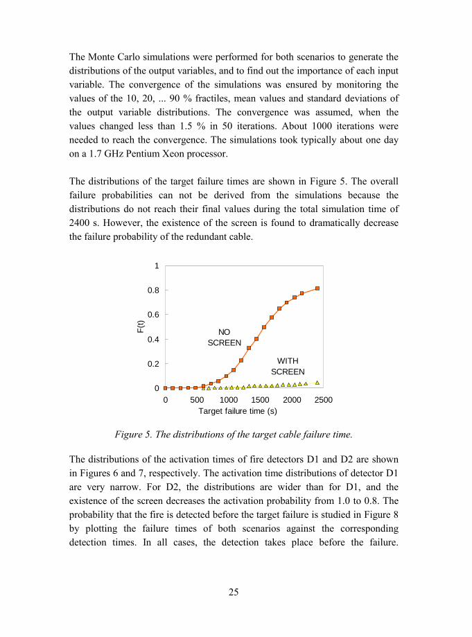
The distributions of the target failure times are shown in Figure 5. The overallfailure probabilities can not be derived from the simulations because thedistributions do not reach their final values during the total simulation time of2400 s. However, the existence of the screen is found to dramatically decreasethe failure probability of the redundant cable.
0
0.2
0.4
0.6
0.8
1
0 500 1000 1500 2000 2500Target failure time (s)
F(t)
WITHSCREEN
NOSCREEN
Figure 5. The distributions of the target cable failure time.
The distributions of the activation times of fire detectors D1 and D2 are shownin Figures 6 and 7, respectively. The activation time distributions of detector D1are very narrow. For D2, the distributions are wider than for D1, and theexistence of the screen decreases the activation probability from 1.0 to 0.8. Theprobability that the fire is detected before the target failure is studied in Figure 8by plotting the failure times of both scenarios against the correspondingdetection times. In all cases, the detection takes place before the failure.

26
However, this does not tell about the probability of the fire extinction becausethe sprinkler reliability and suppression processes are not considered.
0
0.2
0.4
0.6
0.8
1
0 200 400 600D1 activation time (s)
F(t)
WITHSCREEN
NOSCREEN
Figure 6. The distributions of the heat detector D1 activation times. D1 islocated inside the fire room (ROOM 1).
0
0.2
0.4
0.6
0.8
1
0 600 1200 1800 2400D2 activation time (s)
F(t) WITH
SCREEN
NOSCREEN
Figure 7. The distributions of the heat detector D2 activation times. D2 islocated inside the target room (ROOM 3).

27
0
500
1000
1500
2000
2500
0 500 1000 1500 2000 2500Target failure time (s)
D1
activ
atio
n tim
e (s
)
Figure 8. Comparison of D1 activation times vs. target failure times (N = 954).
The sensitivity of the target failure time for the various input variables is studiedby calculating the rank order correlations. These coefficients are showngraphically in Figure 9. The two most important variables are the RHR growthtime and the assumed failure temperature of the target cable. As the distributionsof these two variables do not have a solid physical background, this result can beused to direct the future research. In addition, the length of the virtual fire room(room 1) has a strong correlation with the failure time. In the scenario wherescreen is present, the height of the lower edge of the screen has strong negativecorrelation with the failure time. It is therefore recommended, that the screen,when present, should reach as low as possible to prevent smoke from flowingunder the screen. The rest of the correlations are not statistically significant.

28
Source height
Screen edge height
Critical cable temperature
Room 1 depth
Cable radius
Cable heightCable
conductivity
Detector activation
temperature Tunnel height
Tunnel length
Door height
Cable densityAmbient
temperatureRoom 2 depth
Detector RTI
Tunnel widthVentilation time
constantConcrete density
Door width
RHR Growth time
-0.6 -0.4 -0.2 0 0.2 0.4 0.6Rank correlation for target failure time
S3S4
Figure 9. The sensitivity of the target failure time for the input variables. S3 ="with screen", S4 = "without screen". Here, "room depth" = "room length".

29
4.2 Electronics room fire scenario
As a second example, a fire of an electronics cabinet inside the electronics roomis studied. In their previous study of the similar fire, Eerikäinen & Huhtanen[1991] found that a fire of a single cabinet does not cause direct threat to theother cabinets, in terms of the gas temperature in the compartment. However, itwas noticed already by direct experiments [Mangs & Keski-Rahkonen 1994] thespreading of the fire and conductive heating of the components in the neighbourcabinets as well as the effect of smoke on the electronic components [Mangs &Keski-Rahkonen 2001] may cause failures in the other cabinets of the fire room.Therefore, the probability that the room is filled with smoke during a fire mustbe considered in addition to the temperature increase. The main target variable isthe failure time of a cable inside some other electronics cabinet than the cabinetcontaining the fire. In addition, the convective heating of the neighbouringcabinets is not taken into account, meaning that the distance from the fire to thetarget is sufficiently large.
The fire room is 18.5 m long, 12.1 m wide and 3.0 m high electronics room,containing about 100 electronics cabinets in 12 rows. The room has mechanicalventilation with a constant flow rate (1.11 m3/s) and some additional leakages tothe ambient. Both the ventilation flow rate and the leakage area are taken to berandom variables. Separate cooling devices and smoke circulation through theventilation system are not taken into account, nor is the heat transfer to the roomboundaries. The omission of the cooling devices is known to change thepredicted gas temperature significantly. The results should therefore beconsidered as indicative only.
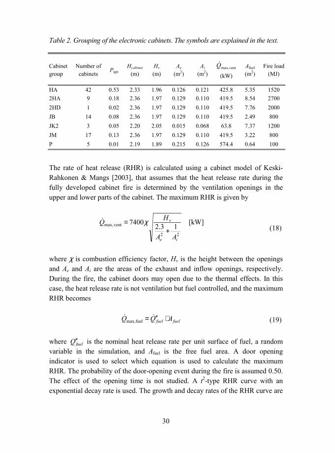
The starting point of the simulation is the collection of the physical data on theelectronic cabinets. The geometrical properties and fuel content of 98 cabinetswere measured. Based on the collected information, the cabinets were groupedinto seven groups, shown in Table 2. The second column shows the number ofcabinets in each group. Pign is the probability, that the ignition takes place in theparticular group, calculated based on the amount of electronic devices (circuitboards and relays) inside the cabinets. Most differences are found in the fuelsurface area Afuel and fire load. As these properties have an effect on the heatrelease rate curve, they are chosen to be distinctive properties like the ventproperties.
30
Table 2. Grouping of the electronic cabinets. The symbols are explained in the text.
Cabinetgroup
Number ofcabinets
PignHcabinet
(m)Hv
(m)Ae
(m2)Ai
(m2)ventmax,Q�
(kW)
Afuel
(m2)Fire load
(MJ)
HA 42 0.53 2.33 1.96 0.126 0.121 425.8 5.35 15202HA 9 0.18 2.36 1.97 0.129 0.110 419.5 8.54 27002HD 1 0.02 2.36 1.97 0.129 0.110 419.5 7.76 2000JB 14 0.08 2.36 1.97 0.129 0.110 419.5 2.49 800JK2 3 0.05 2.20 2.05 0.015 0.068 63.8 7.37 1200JM 17 0.13 2.36 1.97 0.129 0.110 419.5 3.22 800P 5 0.01 2.19 1.89 0.215 0.126 574.4 0.64 100
The rate of heat release (RHR) is calculated using a cabinet model of Keski-Rahkonen & Mangs [2003], that assumes that the heat release rate during thefully developed cabinet fire is determined by the ventilation openings in theupper and lower parts of the cabinet. The maximum RHR is given by
22
ventmax, 13.27400
ie
v
AA
HQ+
= χ� [kW](18)
where χ is combustion efficiency factor, Hv is the height between the openingsand Ae and Ai are the areas of the exhaust and inflow openings, respectively.During the fire, the cabinet doors may open due to the thermal effects. In thiscase, the heat release rate is not ventilation but fuel controlled, and the maximumRHR becomes
fuelfuel AQQ ⋅′′= ��fuelmax, (19)
where fuelQ ′′ is the nominal heat release rate per unit surface of fuel, a randomvariable in the simulation, and Afuel is the free fuel area. A door openingindicator is used to select which equation is used to calculate the maximumRHR. The probability of the door-opening event during the fire is assumed 0.50.The effect of the opening time is not studied. A t2-type RHR curve with anexponential decay rate is used. The growth and decay rates of the RHR curve are

31
random variables in the simulation. The parameters of these distributions aretaken from the experimental works of Mangs & Keski-Rahkonen [1994, 1996].The decay phase starts when 70 % of the fire load is used.
It is very difficult to apply the zone-type fire model to the cabinet fire, becausethe actual source term for the room is the smoke plume flowing out of thecabinet. A reasonable representation of the smoke flow can be found if the baseof the "virtual" fire source is placed close to the half of the cabinet height. Thenthe mass flow of free smoke plume at the height of the cabinet ceiling is roughlyequal to the vent flow. Now, the height of the virtual fire source is considered asrandom variable. A list of the random variables is given in Table 3.
Table 3. A list of random variables used in the electronics room fire scenario.
Distributiontype
Mean Std.dev. Min Max Units
RHR growth time tg Uniform 750 2000 750 2000 sDoor opening indicator Discrete 0 1
RHR Decay time Uniform 800 1400 800 1400 sCabinet type Measured
RHR per unit area fuelQ ′′� Normal 150 40 50 300 kW/m2
Detector RTI Normal 80 10 50 100 (m/s)1/2
Detector activation temperature Normal 57 5 40 100 °CCritical target temperature Normal 80 10 50 200 °CTarget radius Uniform 1 5 mmLeakage area Uniform 0 3 m2
Virtual source height zf/Hcabinet Uniform 0 0.5
Ventilation flow rate Normal 1.11 0.2 0.5 2 m3/s
Four output variables are considered:1. Failure time of the target cable. The cable is located 0.5 m below the height
of the cabinet, therefore simulating a device inside a similar cabinet.2. Smoke filling time: time when the smoke layer reaches the height 2.0 m.3. Smoke filling time: time when the smoke layer reaches the height 1.5 m.4. Smoke filling time: time when the smoke layer reaches the height 1.0 m.
The effect of the observation height is studied by observing the smoke filling atthree different heights. The convergence was ensured in the same manner, as in

32
the previous example. 700 iterations were needed for convergence at this time.The simulation took about 4 hours on a 2.0 GHz Xeon processor. The problemdefinition using an existing tool required a few workinghours. The datacollection and analysis, in turn, took four workingdaysis, being the most timeconsuming part of the process. In planning and collection, the expertise of theplant personnel must be utilized as much as possible.
The distribution of the target failure times is shown Figure 10. Target failuresmay take place after 500 seconds, after which the failure probability increases to0.8. Higher failure probability would be found inside the neighbouring cabinetswith a direct contact to the burning cabinet, and in the ceiling jet of the firegases. These results are inconsistent with the previous findings of Eerikäinen &Huhtanen [1991]. The most obvious reason for the different results is the longersimulation time. The overall simulated period was here 7200 s, while Eerikäinen& Huhtanen stopped their simulation soon after 600 s. At this point our failureprobability is still very small. Other possible reasons for the inconsistency arethe variation of the RHR curve, which may cause very severe conditions in somesimulations, and the omission of the cooling devices.
0
0.2
0.4
0.6
0.8
1
0 1200 2400 3600Target failure time (s)
F(t)
Figure 10. The distribution of the target failure time.
The distributions of the smoke filling times are shown in Figure 11. The smokelayer reaches the height of the electronic cabinets from 500 to 1800 seconds afterthe ignition. The overall probability of getting inside the smoke layer drops from0.8 to 0.2, when the observation height is reduced from 2.0 m to 1.0 m.

33
0
0.2
0.4
0.6
0.8
1
0 600 1200 1800 2400 3000 3600Filling time (s)
F(t)
2.0 m1.5 m1.0 m
Figure 11. The distributions of the smoke filling time.
The sensitivity of the failure time to the input variables is shown in Figure 12.The height of the virtual fire source has the strongest effect on the failure time.This is very unfortunate, because in this particular application it is a numericalparameter. Other important variables are the door opening indicator, RHRgrowth time and the ventilation flow rate. The reliable locking of the cabinetdoors is the most important physical variable that can be directly affected byengineering decisions.
-0.6 -0.4 -0.2 0 0.2 0.4 0.6
Rank correlation for target failure time
Cabinet door opens
Virtual source height
RHR growth time
Ventilation flow rate
Cabinet type
Leakage areaDetector activation temperature
Critical target temperature
Detector RTI
Target radius
RHR decay rate
RHR/fuel area
Figure 12. The sensitivity of the target failure time to the input variables.

34
5. SummaryProbabilistic Fire Simulator is a tool for Monte Carlo simulations of firescenarios. The tool is implemented as a worksheet computing tool, usingcommercial @RISK package for Monte Carlo part. The fire is modelled usingtwo-zone model CFAST. The Monte-Carlo simulations can provide thedistributions of the output variables and their sensitivities to the input variables.Typical outputs are the times of component failure, fire detection and flashover.The tool can also be used as a worksheet interface to CFAST. Extension to theother fire models is possible.
The presented example cases demonstrate the use of the tool. Informationcollected from a nuclear power plant was used for the generation of the inputdistributions in the cable tunnel scenario, which can therefore be considered as arealistic representation of the problem. The results show that the heat detectorgives an alarm before the loss of the redundant cables, with a very highprobability. However, the detector reliability was not considered. According tothe sensitivity measures, the most important parameters for the distribution ofthe failure time of the redundant cable are i) the growth rate of the fire, ii) thescreen providing a physical separation of the burning and target cable trays, iii)the critical temperature of the cable material and iv) the radius (mass) of thetarget cable. The sensitivity information can be used to improve the safety of theredundant cables. For example, the designers can directly affect the location ofthe screen and placing of the different cables inside the tunnels. The distributionsof the growth rate and critical temperature, in turn, are combinations of thelacking information and the range of different scenarios and materials covered inone simulation. Unfortunately, the failure time is also sensitive to the length ofthe virtual room of fire origin, which is a purely numerical parameter. Thisphenomenon should be studied more carefully in the future.
The second example considered an electronic cabinet fire inside an electronicsroom. The procedure of data collection, model development and actualsimulation were described to demonstrate the use of the model in practicalapplications. The data collection and analysis was found the most timeconsuming part of the process. The various ways to enhance this kind of analysisare therefore needed. The simulation results showed that during a fire of a singlecabinet, the thermal environment inside the room might cause a failure of an

35
electronic component inside another cabinet, with a probability of 0.8. Theinconsistency with the earlier studies can be explained with the longersimulation time and the variation of the RHR curve. Due to the strong effect ofthe opening of the cabinet door on the RHR curve, a reliable locking of thecabinet doors is the most important physical variable that can be directlyaffected by engineering decisions.

36
USER'S MANUAL

37
6. Software and hardware requirementsThe Probabilistic Fire Simulator PFS is used on a personal computer havingMicrosoft Windows 95 or higher operating system. PFS has been implementedas a Microsoft Excel workbook. Therefore, Excel 97 or higher is needed. PFSworkbook may be edited by the user, but it is the user's responsibility to save abackup copy of the original workbook.
The PFS workbook contains macros that are used to call CFAST zone model.The workbook also calls some external functions that are distributed as DynamicLink Libraries (DLL). These files are called CableTemp.dll and CallCfast.dll. Touse these DLL's one must have the Fortran type definition file dforrt.dllsomewhere in the computer's path. Care should be taken that the running of themacros is enabled by the macro virus protection utility. Sometimes the calls ofthe external functions cause false virus alarms.
The Monte-Carlo simulations are done using commercial software @RISK1.Version 3.5 of @RISK or higher is needed. @RISK should always be startedprior to opening the PFS workbook. If @RISK is not installed some functions ofthe PFS workbook do not work correctly, and must be replaced by standardExcel functions.
CFAST zone model [Peacock et al. 1993] is needed for the zone modelsimulation. Version 5.0 is recommended, because that allows running thesimulations on the background. However, earlier versions may be used as well.
Any Pentium-based computer with at least 64 MB of memory and 100 MB offree disk space should be enough. However, the software has been tested on veryfew computers so far.
1 @RISK is part of the DecisionTools Suite by Palisade Inc. Information on the softwarecan be found on the company's web site: www.palisade-europe.com
38
7. Definitions@RISK The commercial Monte-Carlo simulation software that works on
Microsoft Excel workbook.
detector In the zone model, detectors are used to represent both sprinklersand actual fire detectors.
distribution function
The statistical distribution used for sampling of a randomvariable. The distribution functions are provided by @RISK.During the Monte-Carlo simulation, these functions return arandom value but during the interactive use, they return the meanvalue of the distribution.
interactive use
The PFS workbook can be used simply as an interface for theavailable fire models. It provides a simple and fast method to useCFAST zone model, for example. @RISK is not needed duringthe interactive use.
output variable
A variable whose value or the distribution of values is the resultsof the simulation. A typical output is a time, when some conditionis met. For example, target failure time, detection time of the fireor time to flashover.
sampling A mathematical algorithm that picks one value randomly from agiven distribution.
target Target is a physical object whose temperature is calculated duringthe fire, and whose failure time is examined. The original purposeof PFS was to study the distribution of the failure time of theredundant cables in cable tunnel fire. This was done by

39
calculating the temperature of the target cable shield andassuming some critical temperature, for example 200 °C. Usermay add other types of targets than just cables. A target has somethermal properties and a physical size and location. All of theseproperties may be random variables.
thermal database
A collection of material properties like material thickness andconductivity needed by CFAST. If any of the material propertiesis a random variable, the database must be generated during everyiteration of the Monte-Carlo simulation.

40
8. Using Probabilistic Fire Simulator8.1 General
The Probabilistic Fire Simulator (PFS) is implemented as Microsoft Excelworkbook. The individual calculation operations are grouped on worksheets. Forexample, the worksheet FireSource contains the analytical formulas andexperimental data that are used to define the rate of heat release (RHR).CableTemperature worksheet in turn is used to combine the results from severalpossible models available for the calculation of the cable temperature.
Although the spreadsheet program updates all the worksheets almostinstantaneously every time some data has been changed, it is useful to define theorder in which the data are used, as a logical way to proceed through thedefinition of the simulation data and the actual simulation. In the followingsections, separate procedures will be presented for the use of PFS as a userinterface for the fire model and the Monte-Carlo simulations. The procedurescorrespond to the PFS workbook in the form as it is distributed. Every user may,and is even encouraged to, modify the workbook, in order take the fulladvantage of the flexibility of PFS.
8.2 Fire model user interface
The PFS workbook can be used as an interface for the CFAST fire modelindependently of the Monte-Carlo feature. It is even possible to use theworkbook without @RISK software, but some changes are then needed to avoidthe Excel -error messages due to the missing @RISK functions. If @RISK is notinstalled, replace the distribution functions (RiskNormal, RiskUniform,RiskGeneral etc.) on RandomVariables worksheet with the values of thecorresponding variables. Also, replace the CurrentIter() function on the Controlworksheet by zero.
The suggested order of the steps needed to do a single simulation is shown as aflowchart in Figure 13. The actual order of the definition steps is not alwayscrucial, but the geometry definition is recommended before the other issues,

41
because the geometry sets some natural limitations for the locations of targetsand detectors.
Define geometry
Define sprinklers /detectors
Define materials
Define RHR curve
Define fire sourceproperties
Define target(cable)
Worksheet Purpose
1. Main Set simulation time2. Control Set models and parameters
1. ZoneModelInput rooms and vents2. RandomVariables room dimensions
1. ThermalDataBase Define wall/ceiling materials2. ZoneModelInput Select material for each room
1. Control Fire type, Max(RHR)2. RandomVariables RHR coefficients3. FireSource New data definitions.
1. RandomVariables height2. ZoneModelInput position, area, species
1. Control target properties2. ZoneModelInput set CFAST target position3. RandomVariables radius, critical temp, height
1. Control type2. RandomVariables RTI, detection temperature3. ZoneModelInput Location
1. Control ForceAutoMode, CallMode2. Macro: RunCfastVB
1. Main temperatures, cable loss timedetection time, etc.
2. GasTemperature, DetectorResults, CableTemperature etc.
Step
Run simulation
Read results
Set parameters
Def
intio
n Se
ctio
n
Figure 13. Suggested order of the steps needed to define the input dataand to do a single fire simulation using PFS.
42
8.2.1 Set parameters
The basic parameters are the total simulation time, found out the Main worksheet,and the various control parameters, found on the Control worksheet. The controlparameters are used to select the physical models for heat release rate and thecalculation of gas and target temperatures. The rooms where the layertemperatures and heights are reported are selected on the ZoneModelInputworksheet, under the TARGET ROOMS keyword.
8.2.2 Define geometry
This step is done by defining the room dimensions, vent dimensions and the ventopening / closing times. The room dimensions can be set by a number ofdifferent ways on the RandomVariables and ZoneModelInput worksheets. Values onthe other sheets are usually linked to the value on the RandomVariables sheet.During the interactive use, the distribution function returns the mean value, andis therefore transparent to the user. As an alternative, the sampling can be donefrom general, measured distributions.
Two vents can be defined between each room. The vent properties are alldefined on ZoneModelInput worksheet, under the HVENT keyword. The openingand closing times can be defined under the CVENT keyword for the first ventonly. The possible second vent is assumed always open. It is also possible to setthe breaking temperature for window glasses Tw. The corresponding vent is thenopened, if the upper layer temperature Tup > Tw, and the layer interface is belowthe window softit, on either side of the window. CFAST, itself, can not handlebreaking windows, but PFS interface will make several runs and open the ventsas the breaking condition is met. However, the comparison of layer interface andwindow soffit heights requires that the rooms are on the same level, ie. HI/F -values are equal.
Mechanical ventilation can be modelled by defining fans between the rooms.The connection points (nodes) and fan properties are all defined onZoneModelInput worksheet, under the MVOPN and MVFAN keywords,respectively. Each node must have a room where it is located and orientation.The flow-pressure curve of the fan is modelled using a constant value. The
43
number of fans must be less than seven. The fans are typically used to definemechanical smoke ventilation system. The second room is then set to theambient. Actually, CFAST allows the modelling of a complete ventilationnetwork with fans and nodes, but here only the fans are used to keep theinterface simple.
8.2.3 Define materials
If the ceiling and wall materials are varied, or the heated target is modelled usingCFAST target utility, the thermal database should be generated for everysimulation. The following steps are needed to use this functionality:
1. On the Control worksheet, under CFAST control section, set CreateThDbvariable TRUE. By default this variable should be FALSE, because thewriting of the thermal database file slightly slows the Monte-Carlosimulation. The thermal properties are then read from the file defined onZoneModelInput worksheet that must exist in the CFAST directory.
2. The material properties are defined on the ThermalDataBase worksheet. First,the number of used materials is set. It should be between 1 and 20. Use onlyas many materials as you need to minimise the size of the thermal databasefile. The target material, for example PVC, is usually defined on the firstrow of the database. The material properties can be connected to randomvariables, sampled at the RandomVariables worksheet.
3. The building materials are selected on the ZoneModelInput worksheet. Thename of the existing database file should be given without the file nameextension .df. The wall and ceiling materials are selected under the CEILIand WALLS keywords with the number of corresponding material in thethermal database. If all the cells are left blank, all the ceilings (or walls) areassumed adiabatic. On the other hand, if any of the cells has a value, theblank cells (or walls) will have the properties of concrete.

44
8.2.4 Define RHR curve
To define the rate of heat release (RHR) curve it is necessary to define the firetype and maximum value of RHR. The maximum value is needed for theanalytical RHR curves to prevent the unphysical situations. The fire type isselected at the Control worksheet. The fire types, the data source and possibleparameters are listed in Table 4. Type 1 is the typical design fire with t2-typegrowth [Heskestad & Delichatsios 1977, NFPA 1985], and an exponential decay[Keski-Rahkonen 1993].
For special scenarios RHR data may be taylored from local constraints, whichmay differ radically from these general trends. The actual RHR data is stored onthe FireSource worksheet. This is the place to add new RHR curves.
Table 4. Fire types and the corresponding parameters defined in PFS.
Index Type Parameter0 Constant RHR RHR1 t2-type ( )[ ]ddg ttttQtQ τ/)(exp(10,/10,min)( 323
max −−⋅⋅= �� ,
where tg is the growth time, td is the decay start time and τd is thedecay time constant, [Keski-Rahkonen 1993, Linkova & Keski-Rahkonen 2002, Linkova et al. 2003].
tg, td, τd
2 Fire area grows at constant flame front velocity vfl. vfl
4 Experimental RHR of horizontal cable trays, measured by Mangs &Keski-Rahkonen [1997].
101-114 Experimental RHR curves of household appliances, measured byHietaniemi et al. [2001]101-104 Dish washers105-107 Washing machines108-111 Refridgerator-freezers112-114 TV sets
201-205 Experimental RHR curves of smoke detector test fires, measured byBjörkman & Keski-Rahkonen [1997]201 TF1, open cellulosic fire202 TF2, smouldering wood203 TF3, glowing cotton204 SPVC205 FPVC

45
301-306 Experimental RHR curves of electronic cabinets, measured by Mangs& Keski-Rahkonen [1994]. Experiments 1, 2C, 3, 4, 5 and 6B
8.2.5 Define fire source properties
Besides the RHR curve, the fire source has the following properties: position,area, compartment of origin and the species yields. The height of the fire sourcecan be controlled from the RandomVariables worksheet, as it one of the mostimportant properties. Other properties are defined on the bottom of theZoneModelInput worksheet.
The yields of two species can be given. By default they are OD (soot) and CO.One value is given for both species, and the value is kept constant trough thefire. The calculation of the ceiling jet flows is controlled by the CEILI keyword.Usually it can be given a value "ALL". The fire area is assumed linearlyproportional to the RHR with maximum value defined at the "Maximum FireArea" cell. However, this variable has usually very small effect to the simulationresults. A detailed description of the parameters is given in the CFAST manual.
8.2.6 Define target
The properties of the target, for example cable, are mainly controlled atRandomVariables and Control worksheets. To summarise, some of the targetproperties (radius, critical temperature and relative height) are shown on the Mainworksheet, while most of the properties are defined on the Control worksheet.
The first parameter of the Target temperature �section at the Control worksheet isthe model index. The following models are available at the moment:
Index Target temperature model
0 Time constant. Cable temperature follows gas temperature with atime constant depending on the cable size and thermal properties.This model has shortest possible calculation time, but it is accurateonly for very thin cables.

46
1 Analytical cable model. The cable shield temperature is calculatedbased on the analytical solution of the axisymmetric heat transferequation. Also quite fast, but the accuracy is not guaranteed.
2 CFAST/Target The heating of the target can be modelled using theCFAST target utility, which allows the heat transfer calculation of 1Dheat transfer inside the zone model. This method is very useful, as itallows the contribution of the radiative heat transfer, which is verydifficult to calculate outside the zone model. The target material isselected at ZoneModelInput worksheet by typing the index of thecorresponding material in the thermal database to the "Material #"column, under the TARGET keyword. Usually the first material of thethermal database is reserved for targets. The heating of theaxisymmetric objects, like cables, can be approximated by setting thematerial thickness to R/(2π), where R is the cable radius.
3 FEM. The most accurate solution to the cable heat transfer equationcan be obtained by 1D Finite Element Method (FEM), including boththe insulator shield and the metal core of the cable. The gastemperature is used for the boundary condition on the cable surface.
4 FEM/target. This method is an experimental version. The FEMmethod is used to solve the cable heat transfer, but the boundarycondition is taken from the target boundary heat flux given byCFAST. The model should not be used.
The results given by the methods 1 to 4 are compared in Figure 14, showing thefailure time distributions for some t2-type fire and relatively thin cable. It can beseen that the analytical model and FEM give very similar distributions, butCFAST target gives clearly smaller failure times. This is probably due to theradiative heating. The FEM/target option is shown to give very different results,and are considered wrong.

47
0
0.2
0.4
0.6
0.8
1
0 200 400 600 800 1000 Time (s)
F(t)
AnalyticalTargetFEMFEM/Target
Figure 14. Comparison of the different target (cable) heating models.
8.2.7 Define sprinklers and detectors
The modelling of the heat detectors is a well-established procedure, and thereliability of the detection time predictions can be considered reliable. Themodelling of the smoke detectors is still under active research, and this utilityshould be used with caution. Heat detectors represent both sprinklers and actualheat detectors.
The detector parameters are summarised on the Main worksheet. Theseparameters include detector type (1 for smoke, 2 for heat), operation temperatureand RTI. As the modelling of the smoke detectors is developed further, it will bepossible to add delay parameters of the Weibull distribution describing thedistribution of penetration delays. Usually these parameters depend on thedetector type and flow velocity. Detector location, consisting of the roomnumber and physical co-ordinates, are defined on ZoneModelInput worksheet,under the keyword DETECT. All the variables can be linked to random variabledistributions at RandomVariables worksheet.
48
8.2.8 Run simulation
First, set the simulation and CFAST parameters on the Control worksheet. Theseparameters are mainly used for debugging purposes. By setting"ForceAutoMode"�variable to 1 user may force the CFAST to run every timethe workbook is updated. The default is 0. DTCHECK-parameters at the"CFAST control" section control the critical time step size of CFAST solver."CallMode" parater controls whether the temporary files are deleted afterCFAST simulation or not. Normally (value 0) all the files are deleted, but in thedebug mode (value 1) left on the hard disk.
The actual simulation is started by running a macro RunCfastVB. It can befound under the Tools/Macro �menu of Excel.
8.2.9 Read results
The simulation results (time series) are organised to various worksheets,depending of the type of the data. For example, gas temperature data are foundat the GasTemperature worksheet, detector data at the DetectorResults worksheetand cable temperature at the CableTemperature worksheet. Some scalar values,like the target failure times are calculated as table lookups at the "Main"worksheet. All the data read from the CFAST results are found at CallCfastworksheet. Most of the results are shown as time series. One exception is thedetector operation times, which are reported in the cells just above thecorresponding detector temperature time series.

49
8.3 Monte-Carlo simulation
The suggested order of the steps needed to carry out a Monte-Carlo simulation isshown as a flowchart in Figure 15. The purpose and means of the individualsteps are described below.
8.3.1 Start @RISK
The first step of the Monte-Carlo simulation use of PFS, is to start @RISKsoftware. See the @RISK manual for details. @RISK automatically startsMicrosoft Excel, enabling the statistical functions and opening two customtoolbars. These toolbars can be used to define @RISK inputs and outputs, open@RISK simulation settings panel, and to open other Decision Tools �softwareapplications.
8.3.2 Open PFS workbook
PFS is implemented as a Microsoft Excel workbook. To start a new simulationproject, open an existing workbook, and save it with a new name. Always keepa backup copy of the original workbook!
8.3.3 Definition section
The definition of the fire scenario and the selection of the physical modelsfollow the steps shown in the definition section of Figure 15.

50
Definition section
Define outputvariables
Define randomvariables
Where Purpose
Windows utility Load @RISK functions forExcel
Excel File/Open Create the physical modellingenvironment
See Figure 1. Definition of the physicalscenario, selection of theapplied models etc.
1. RandomVariables Random variables aredefined using the @RISKdistribution functions.
2. ZoneModelInput Input value are linked to therandom variables.
1. Main The output variables (failuretime, detection time etc. areselected for @RISK.
2. Other worksheets Optional outputs, like timeseries
@RISK utility Set number of iterations ORthe convergence criteria
@RISK utility (Start simulation -button)
@RISK utility Statistics, output distributions
Step
Run simulation
Read results
Start @RISK
Open PFSworkbook
Set simulationparameters
Figure 15. Suggested order of steps needed to do Monte-Carlo simulation withPFS.

51
8.3.4 Define random variables
The definition of the random variables is what makes the fire simulation of aMonte-Carlo simulation. In practice it means that the value of some physicalvariable is calculated by @RISK as a sample from some statistical distribution.During the interactive use of the workbook, the distribution function returns themean value of the distribution. The distribution functions are defined on theRandomVariables worksheet.
Some examples of the statistical distribution functions, that are available in@Risk 3.5, are listed in Table 5. See @RISK documentation for otherdistributions. The corresponding worksheet functions, used in Excel, have aprefix "Risk". Possible functions are, for example, RiskNormal(6.2,2.0) andRiskUniform(0,1). In practice, the distribution parameters are linked to the othercells of the PFS workbook.
Table 5. Examples of the statistical distribution functions available in @RISK 3.5.
Function Returns
CUMUL(minimum,maximum,{X1,X2,...,Xn},{p1,p2,...,pn})
cumulative distribution with n points between minimumand maximum with cumulative probability p at eachpoint
DISCRETE({X1,X2,...,Xn},{p1,p2,...,pn})
discrete distribution with n possible outcomes with thevalue X and probability weight p for each outcome
LOGNORM(mean,standarddeviation)
lognormal distribution with specified mean and standarddeviation
NORMAL(mean,standarddeviation)
normal distribution using mean and standard deviation
TNORMAL(mean,std.deviation,minimum,maximum)
normal distribution truncated at minimum and maximum
UNIFORM(minimum,maximum) uniform distribution between minimum and maximumWEIBULL(alpha,beta) weibull distribution with shape parameter alpha and scale
parameter beta

52
8.3.5 Define output variables
To collect the statistics of the interesting output variables, they must be definedas @RISK outputs, by selecting the corresponding cell, and pressing the"Output" -button of the @RISK toolbar. Typical outputs are the failure time ofthe target(s) and detector activation time. It is possible to define a time series,like gas temperature, as output.
8.3.6 Set simulation parameters
The parameters of the Monte-Carlo simulation are set on the @RISK simulationsettings panel, opened by pressing the "Change @RISK settings" button in the@RISK toolbar. The following parameters are usually set:
Iterations tab: # Iterations = 300. This setting has no effect, if theauto-stop feature is used (recommended).
Update display. This setting must be selectedwhen using CFAST or other external model!Otherwise, the output variables are not saved.
Sampling tab: The sampling type = Latin Hypercube. However,Monte-Carlo sampling should be used if there aredefined correlations between the input variables.
Standard Recalc = Mean value.
Convergence tab: Monitor convergence should be selected, andchecking frequency set to 50 (smallest possiblevalue).
Auto-Stop should be selected, with a convergencecriterion of 1.5 %. This ensures that the Monte-Carlo iterations are continued until the outputstatistics are well converged.

53
8.3.7 Run simulation
The Monte-Carlo simulation is started by pressing the "Run simulation" buttonof the @RISK toolbar.
During the simulation, the CFAST-console is opened on the screen, typicallyhundreds of times (if CFAST -fire model is used). This makes it practicallyimpossible to use the computer for any interactive work during the simulation.
8.3.8 Read results
The output statistics are studied by opening the @RISK main window. Press"Open @RISK Main Window" -button in the @RISK toolbar.
For each output variable, @RISK reports the mean value, standard deviation andseveral fractiles. The graphical output can be used to plot the distribution of theoutput variable. The graphs can be exported to a separate Excel workbook.

54
9. Input variables and parametersThis section describes the purpose of the input variables and parameters foundon each worksheet. Some guidance on the use of these parameters is also given.
9.1 Main
The Main worksheet contains only one input variable: MAXIMUM TIME, whichis the maximum simulation time (s) in all the simulations. It should be setapproximately equal to the maximum expected value of the output variables. Iftoo short, the tail of the time distribution can not be calculated. If too long, theresolution of the time series becomes poor (resolution = maximum time / 100).
Some of the most important input parameters are summarised on the worksheetto provide a simple way to check their values. The actual distributions aredefined elsewhere in the workbook.
9.2 Control
The Control worksheet contains a number of parameters that are used to choosebetween various physical models and fire sources, set numerical parameters ortarget properties. The parameters are organised to the following groups:
Fire
Type Selects the fire source type. These types are listed inTable 4.
RHR Limiter Upper limit of the rate of heat release (kW). Thisparameter is used to define the constant phase of theRHR curve. It is also used to avoid unphysical RHRvalues, that could slow the execution of the zonemodel.
RHR/fuel area Rate of heat release per fuel surface area (kW.m-2).This parameter is used, if the RHR curve is defined by

55
flame spread velocity (type 2).
Gas temperature
Model Selects the fire model. 0 = constant gas temperature, 1= Alpert's ceiling jet model, 3 = CFAST.
Constant Constant gas temperature (°C), used if Model = 0.
Sprinkler/DetectorControl
Type Type of the fire detectors: 1 = smoke detector and 2 =heat detector. For smoke detectors, the detectortemperature follows the corresponding ceiling jettemperature exactly. This models the operation of adetector with RTI = 0, and having no thermal inertia.
Sprinkler A flag that is used to set the water flux on after thedetection. If 0, the detector does not try to suppress thefire. This is the suggested choise, because thesuppression feature of CFAST does not work correctly,so far.
Target temperature
Model Selects the heat transfer model for the targettemperature calculation. 0 = time constant (lag), 1 =analytical cable model, 2 = CFAST target, 3 = FEMwith gas temperature boundary condition, 4 = FEMwith CFAST target heat flux boundary condition (notrecommended).
General
Initial temperature Initial target temperature (°C).
Heat transfer coeff. Convective heat transfer coefficient (W.K-1m-2) of thetarget cable.
Insulation properties
Emissivity Cable surface emissivity.
Conductivity Thermal conductivity of the cable insulation material

56
(W.K-1m-1).
Density Density of the cable insulation material (kg m-3).
Specific heat Specific heat of the insulation material (J.kg-1K-1).
Core properties
Radius Radius of the cable core (m).
Conductivity Thermal conductivity of the cable core material(W.K-1m-1).
Density Density of the cable core material (kg.m-3).
Specific heat Specific heat of the cable core material (J.kg-1K-1).
Parameters of theanalytical model
Niter Number of iterations. Typically from 1 to 3. Larger thenumber, more time it takes.
Nroots Number of terms (roots) used in the series. Can be 1, 310 or 30.
CFAST control
DTCHECK Time step size control parameter for CFAST. Does notseem to work properly in CFAST 4.1. That is, CFASTdoes not stop if the time step is smaller than xval forlonger than nsteps.
CallMode 0 for normal use, 1 for debug purposes. In debugmode, the temporary files are not deleted from theCFAST directory.
ThDbCreate Flag to control the use of thermal database. If TRUE,thermal database is written on every iteration. Must be setTRUE, if any of the thermal properties is random variable.
Simulation control
Force Auto Mode Used for debug purposes. If set to 1, CFAST isautomatically called every time, the workbook isupdated, ie. any of the cells is changed.

57
9.3 Random Variables
The RandomVariables worksheet contains the actual distribution functions. Bydefault, 20 independent variables can be defined. The function definitions shouldbe located in the "Input" -column. The parameters of the distribution arecollected on the same worksheet. In case of dimensionless random variables, theactual dimensional variable can be calculated in the right most column. It is theuser's responsibility to link the zone model input variables and target propertiesto the cells of the "Input" -column.
Below are listed some variables that are often defined on this worksheet:
Ambient temperature Distribution of the ambient temperature (°C).
Cable Radius Distribution of the cable radius (mm).
Critical cabletemperature
Distribution of the critical surface temperature (°C),where the target is lost.
Detection penetrationparameter
Distribution of the time lag parameter (s), used inthe statistical detector model.
Detector activationtemperature
Distribution of the operation temperature of the firedetector (°C). For heat detector, this is the trueoperation temperature. For smoke detectors, nowell-established value exists.
Detector RTI Distribution of the response time index of thedetector ( sm / ).
Relative cable height Distribution of the relative (dimensionless) targetheight, defined as ztarget/H.
Relative source height Distribution of the relative (dimensionless) heightof the fire source, defined as zfire/H.
RHR Decay rate Distribution of the decay rate τd.
RHR Decay start Distribution of the starting point td of the decayperiod of the t2-type RHR curve.
RHR Growth time Distribution of the growth time parameter tg (s),used in the t2-type RHR curves. This parameter can

58
serve in other purposes too, depending on theselected fire source type.
ROOM DEPTH Depth of the fire room (m). In tunnel geometry, thisis the length of the tunnel. It should be at least fourtimes the room width.
ROOM HEIGHT Height of the fire room (m). General room heightdistribution can be used.
ROOM WIDTH Width of the fire room (m). General room widthdistribution can be used instead of analyticaldistributions.
9.4 Zone Model Input
This worksheet contains data that is specific to the zone models, especiallyCFAST. To understand the way that the data are organised, user should befamiliar with the format of the CFAST input files.
Most of the data on this worksheet is already defined elsewhere in the PFSworkbook. It is the user's responsibility to link the cells to the randomdistributions or other input sections.
TARGET ROOMS These numbers determine the rooms where thelayer heights and the zone temperatures arereported.
NROOMS Number of rooms in the model.
DAT file The name of the CFAST input file.
HI file The name of the CFAST history file.
Thermal DB The name of the CFAST thermal database file,without the ".db" extension.
Maximum Run Time This parameter is used to limit the CFASTexecution time, to stop simulation in cases where

59
CFAST solver has locked itself to the very stillequations. Cfast is stopped after the given numberof seconds. It should be large enough, that theslowest of the normal simulations can beexecuted. The default is 600 s.
TIMES Print = interval of text outputDisplay = interval of graphical outputOnly one of these intervals should be greater thanzero.
History determines the temporal accuracy of theresults. Usually 1 s is used, but it can be madesmaller to reduce the size of the history file.
TAMB Ambient conditions inside the structure.
EAMB Ambient conditions outside the structure.
HI/F Height of the floor for each room (m).
WIDTH, DEPTH, HEIGH The dimensions of the rooms (m).
CEILI This index determines the ceiling material foreach room. The integer number should correspondto the material numbers of the thermal database. Ifleft blank, gypsum properties are used. If all thecells of the row are blank, ceilings are consideredadiabatic.
WALLS This index determines the wall material for eachroom. The integer number should correspond tothe material numbers of the thermal database. Ifleft blank, gypsum properties are used. If all thecells of the row are blank, walls are consideredadiabatic.

60
HVENT
The vents between the rooms are defined as connection matrices, under keywordHVENT. Two vents can be defined between each room. Actually, CFAST canhandle four, but the limit of two was accepted to keep the PFS interface simple.The first vent is defined by defining the vent dimensions in the upper triangle ofthe connection matrix, and second vent in the lower. If the cell is blank in allthree matrices, the vent does not exist.
Width The vent width (m).
Soffit The height of the vent soffit (upper frame) measuredfrom the first room floor.
Sill The height of the vent sill (lower frame) measuredfrom the first room floor.
CVENT
The first vent can be opened and closed once during the simulation. The openingtime should be given in the upper triangle of the CVENT matrix, and closingtime in the lower triangle. If the both cells are blank, the corresponding vent isalways open. The element should correspond to the elements of the HVENTmatrices. The second vent is always open.
As an alternative, the vent can be defined to be opened when the windowbreaking condition is met (Tup > Tw and Zi < soffit height). To use breakingcondition, set the opening time of the vent to a negative number. The breakingtemperature is set above the CVENT matrix. The default value is 200 ºC.
TARGETS
NTargets The number of targets in the simulation. NTargets shouldbe an integer, from 0 to 3.
Room # The index of the room, where the target is located.
X (m) The x-coordinate of the target (m). (Corresponds to thedepth of the room.)

61
Y (m) The y-coordinate of the target (m). (Corresponds to thewidth of the room.)
Z (m) The z-coordinate (height from the floor) of the target (m).
Normal XNormal YNormal Z
The components of the target surface normal vector (m).
Material # The target material determined as an index to the thermaldatabase.
DETECTORS
NDetectors Number of detectors in the simulation. Integer from 0 to 6.
Type 1 for smoke detector, 2 for heat detector
Room # The index of the room, where the detector is located.
Tactiv (K) Activation temperature (°C).
X (m) The x-coordinate of the detector (m). (Corresponds to thedepth of the room.)
Y (m) The y-coordinate of the detector (m). (Corresponds to thewidth of the room.)
Z (m) The z-coordinate (height from the floor) of the detector(m).
RTI The response time index of the detector ( sm / ).
Sprinkler 0 for detector only, 1 for sprinkler.
Spray density The water spray density of the sprinkler (m/s).
FANS
Nfans Number of fans in the simulation. Integer from 0 to 6.
1st room The index of the upstream room.

62
Orientation 1 for horizontal orientation (typical for ceiling openings),2 for vertical orientation
Height The vertical height of the node, from the 1st room floorlevel (m).
2nd room The index of the downstream room.
Orientation The orientation of the second node.
Height The vertical height of the node, from the 2nd room floorlevel (m).
Area The opening area of the nodes.
Pmin The minimum pressure, under which the flow is constant(Pa).
Pmax The maximum pressure, over which the flow goes to zero(Pa).
Flow The constant flow rate (m3s-1).
CHEMI
Molar weight The weight of the fuel molecule in amu (C = 12).
Humidity The relative humidity of the atmosphere (%).
LOI The limiting oxygen index of the fuel. This is the smallestoxygen concentration (%) where the combustion can takeplace.
-∆Hc The heat of combustion for the fuel (J kg-1).
T(fuel,init) The initial fuel temperature (K).
T(ign, gas) The ignition temperature of the gaseous fuel (K).
Radiative fraction The radiative fraction of the rate of heat release. Usuallyabout 0.3.
LFBO Index of the compartment of fire origin.
FPOS The co-ordinates of the fire inside the compartment. Xcorresponds to depth, Y to width and Z to height.

63
CJET String that determines which ceiling jets are to becalculated. Usually CJET should be ALL.
Maximum firearea
The maximum area of the fire (m2). The time dependentarea is proportional to RHR.
SPECIES
It is possible to define the yield of two species. Actually, CFAST can handleseven, but the limit of two was accepted to keep the PFS interface simple. Thepossible species are HCN, HCL, HCR, CT, O2, OD (optical density = soot) andCO. The species are selected by writing the corresponding strings under thekeywords Specie1 and Specie2. The yields are assumed to constant in time, andtherefore only the first value is given.
9.5 Distributions
It is possible to use general distributions for the sampling of the randomvariables. Distributions worksheet is reserved for the definition of thesedistributions. The general distribution is defined as a set of value-probabilitypairs.
9.6 Thermal Database
Thermal database consists of up to 20 rows of material data. The number ofmaterials is defined first. The number of materials should be kept as small aspossible to minimise the execution time. For some reason (which is stillunknown) CFAST does not accept the last material of the database.Consequently, the last row of the database should not be used!
Each row of the material database contains the following data. At the moment,the material can only have one layer, although CFAST can handle up to 3 layers.A description of the material can be written on the right side of the material datatable.

64
Name The material name should be a string of up to 8characters.
Conductivity (W/Km),Specific heat (J/kgK),Density (kg/m3)
The thermal properties.
Thickness The thickness of the material layer (m).
Emissivity Surface emissivity.
Coefficients of HCLdeposition

65
10. Modifying PFS10.1 PFS Workbook
The workbook has two major modes: Interactive use and non-interactive use.Interactive use means the case where user sets the input variables and explicitlyruns the CFAST calling routine CallCfastVB. Non-interactive use means theMonte-Carlo simulation. The mode is detected on the Control workbook, underSimulation Control. CurrentIter() is a @RISK function returning the iterationnumber. If zero, we are using PFS interactively, and the ControlInterActiveModevariable is set to TRUE.
To find out if the CFAST can be called, the code must check the status of therandom distribution page. This is done by computing a sum of the randomvariables, and referring to that sum in the equation of the ControlDoFunCallvariable on the Control worksheet. Consequently, ControlDoFunCall is set toTRUE, if that sum has been updated (all the variables have been sampled] andthe ControlInteractiveMode is FALSE.
The actual CFAST calling is done on the CallCfast worksheet. The columns fromAN to BV form a variable CfastResArray, which is written by the CallCfastVBsubroutine. In ControlDoFunCall variable is TRUE, the same result is written tocolumns BX - DF, by the CallCfastFun function. Finally, the data is collected tothe first columns B - AL.
Another point, where direct function calls are used is the CableTemperatureworksheet. There the CableTempPL function is called to calculate thetemperature rise of the axisymmetric cable. The function is located in theCableTemp.dll and all the input data is passed as arguments.
The array functions are typed by painting the array, typing the formula, andpressing Ctrl+Shift+Enter.
66
10.2 Visual Basic functions and subroutines
The PFS workbook contains the following Visual Basic functions andsubroutines:
FirstLookup A simple lookup function which interpolates thelookup result between the data points. Not used atthe moment.
CallCfastFun A function that calls a Fortran function CallCfastFun(in CallCFast.dll), which then actually calls CFAST.CallCfastFun has no arguments. In case of breakingwindows, the function has a loop that callsWriteCfastDataFun and CallCfast functions until allthe windows have broken or remained closed.
CallCfastVB A subroutine that only calls CallCfastFun andwrites the result to the worksheet. This is neededbecause the functions are not directly available forinteractive calling.
WriteCfastDataVB A subroutine that provides an interactive access tothe WriteCfastDataFun function.
WriteCfastDataFun A non-interactive function that reads input datafrom the workbook and then send the data to theFortran function WriteCfastData (in CallCfast.dll).
The arguments are the OverRideCVENT flag, andCVENTIN array. They are used to update the ventopening time array CVENT during the callingloop.
MatrixCopy This subroutine is used to copy a two dimensionalarray.

67
10.3 Fortran functions
The actual data writing, CFAST calling and the reading of the results is done byFortran functions. These functions are normally provided as dynamic linklibraries (DLL). The source code of the functions can be provided if needed.However, these functions should be modified only by an advanced user, becausethe passing of the arguments between Visual Basic and Fortran, or Excel andFortran, is very complicated.

68
ReferencesBjörkman, J. & Keski-Rahkonen, O., 1997. Full-scale experiments withdifferent smokes. VTT Publications 332, VTT, Espoo. 18 p. + app. 62 p.
Carlslaw, H.S. & Jaeger, J.C., 1959. Conduction of Heat in Solids.Clarendon Press, Oxford, Second Edition. 510 p.
CIB W14, 1986. Design Guide Structural Fire Safety, Workshop CIBW14. Fire Safety Journal, Vol. 10, No. 2, pp. 75�137.
Drysdale, D., 1985. An Introduction to Fire Dynamics. Wiley, Chichester.424 p.
Eerikäinen, L. & Huhtanen, R. 1991. Ydinvoimalaitoksen huonetilapalo,Loviisa 1:n valvomorakennuksen huonetilan palon numeerinen tarkastelu.STUK-YTO-TR 30. Helsinki. 59 p. + app. 26 p.
Ferson, S. & Ginzburg, L.R. 1996. Different methods are needed topropagate ignorance and variability. Reliability Engineering and SystemSafety, Vol. 54, pp. 133�144.
Haider, C., Hofer, E., Kloos, M., Peschke, J., Röwekamp, M. &Tuerschmann, M., 2002. Unsicherheitsanalysen zu einem Kabelbrand-szenario in Sicherheitsbehälter einer Konvoi-Anlage. GRS - A - 2889,Technischer Bericht, Reaktorsicherheitsforschung-Vorhabens Nr. RS1112. Gesellschaft für Anlagen und Reaktorsicherheit (GRS) mbH. 66 p.
Hannus, M. 1973. Numerical analysis of structural reliability. Helsinki,VTT. Technical Research Centre of Finland, Building Technology andCommunity Development, Publication 5. 1973. 24 p.
Helton, J.C. & Burmaster, D.E., 1996. Guest editorial: treatment ofaleatory and epistemic uncertainty in performance assessment forcomplicated systems. Reliability Engineering and System Safety, Vol. 54,pp. 91�94.

69
Heskestad, G. & Delichatsios, M. A. 1977. Environments of FireDetectors. Phase 1. Effect of Fire Size, Ceiling Height and Materials.Volume 2. Analysis. NBS GCR 77�95, National Bureau of Standards,Gaithersburg, MD. 129 p.
Hietaniemi, J., Mangs, J. & Hakkarainen, T., 2001. Burning of ElectricalHousehold Appliances. An Experimental Study. VTT Research Notes2084. VTT Building and Transport, Espoo. 60 p. + app. 23 p.
Hofer, E. 1999. Sensitivity analysis in the context of uncertainty analysisfor computationally intensive models. Computer Physics Communications,Vol. 117, pp. 21�34.
Hofer, E, Kloos, M., Krzykacz-Hausmann, B. Peschke, J. & Sonnenkalb,M. 2001. Methodenentwicklung zur simulativen Behandlung derStochastik in Probabilistischen Sicherheitsanalysen der Stufe 2. GRS - A -2997, Abschlussbericht, Reaktorsicherheitsforschung Projekt No: RS1111. Gesellschaft für Anlagen und Reaktorsicherheit (GRS) mbH. 229 p.
Hofer, E, Kloos, M., Krzykacz-Hausmann, B. Peschke, J. & Woltereck,M. 2002. An approximate epistemic uncertainty analysis approach in thepresence of epistemic and aleatory uncertainties. Reliability Engineeringand System Safety, Vol. 77, pp. 229�238.
Keski-Rahkonen, O. 1993. Design fire construction for individual assessment.In: Twilt, L. (ed.) Proceedings of 3rd CIB/W14 Workshop "Modelling", 25�26January 1993. TNO, Rijswijk, The Netherlands. Pp. 43�48.
Keski-Rahkonen, O. & Hostikka, S. 1999. Theory versus experiment �Did you forget design of experiment and data reduction? StructuralMechanics in Reactor Technology 15, Post Conference Seminar No. 6,Fire Safety in Nuclear Power Plants and Installations, Munich-Garching,Germany, September 6�7. 21 p.

70
Keski-Rahkonen, O., Mangs, J. & Turtola, A. 1999. Ignition of and firespread on cables and electronic components. VTT Publications 387.Technical Research Centre of Finland, Espoo. 102 p. + app. 10 p.
Keski-Rahkonen, O. & Mangs, J. 2003. Quantitative determination ofsource terms from fires in electronic cabinets: Maximum rate of heatrelease, minimum rate of heat release needed for flashover, and effluentyields from incomplete combustion. Submitted to Fire Safety Journal.
Korpela, K. and Keski-Rahkonen, O., 2000. Fire Loads in OfficeBuildings. In: Proceedings, 3rd International Conference on Performance-Based Codes and Fire Safety Design Methods, 15�17 June 2000, LundUniversity, Lund, Sweden. Pp. 278�285.
Linkova, P. & Keski-Rahkonen, O., 2002. Palon hiipumisaikavakionmäärittäminen [Determination of decay time constants of fires].Palontorjuntatekniikka (2002) No. 1, pp. 12�14, (in Finnish).
Linkova, P., Kaustinen, R. & Keski-Rahkonen, O., 2003. Decay timeconstants of heat release rate, (to be published).
Magnusson, S. E., 1997. Risk Assessment. In: Hasemi, Y. (ed.).Proceedings of the Fifth (5th) International Symposium. March 3�7,1997, Melbourne, Australia, International Association for Fire SafetyScience, Boston, MA. pp. 41�58.
Mangs, J. & Keski-Rahkonen, O. 1994. Full scale fire experiments onelectronic cabinets. Espoo, Technical Research Centre of Finland. VTTPublications 186. 50 p. + app. 37 p.
Mangs, J. & Keski-Rahkonen, O. 1996. Full scale fire experiments onelectronic cabinets II. Espoo, Technical Research Centre of Finland. VTTPublications 269. 48 p. + app. 6 p.

71
Mangs, J. & Keski-Rahkonen, O. 1997. Full-scale fire experiments onvertical and horizontal cable trays. Technical Research Centre of Finland.VTT Publications 324. Espoo, 58 p. + app. 44 p.
Mangs, J. & Keski-Rahkonen, O., 2001. Acute Effects of Smoke fromFires on Performance of Control Electronics in NPPs, Paper No. M1804.In: Matzen,V.C. and Tung, C.C. David (eds.). Transactions � 16th
International Conference on Structural Mechanics in Reactor Technology,Washington DC, August 12�17, 2001. 8 p.
McCormick, N. 1981. Reliability and risk analysis - methods and nuclearpower applications. Academic Press, New York, N.Y. 446 p.
McKay, M.D., Beckman, R.J. & Conover, W.J. 1979. A comparison ofthree methods for selecting values of input variables in the analysis ofoutput from a computer code. Technometrics, 21(2), pp. 239�245.
NFPA, 1985. NFPA 204M, Guide for Smoke and Heat Venting, NationalFire Protection Association, Quincy, MA.
Parry, G.W., 1996. The characterization of uncertainty in ProbabilisticRisk Assessments of complex systems, Reliability Engineering andSystem Safety, Vol. 54, pp. 119�126.
Paté-Cornell, M.E., 1996. Uncertainties in risk analysis: Six levels oftreatment, Reliability Engineering and System Safety, Vol. 54, pp. 95�111.
Peacock, R.D., Forney, G.P., Reneke, P., Portier, R. & Jones, W.W. 1993.CFAST, the Consolidated Model of Fire Growth and Smoke Transport.Gaithersburg, National Institute of Standards and Technology, NISTTechnical Note 1299. 118 p. + app. 116 p.
Pebesma, E.J. & Heuvelink, G.B.M. 1999. Latin hypercube sampling ofmultigaussian random fields. Technometrics 41(4), pp. 303�312.
Spiegel, M.R. 1980. Theory and problems of probability and statistics �SI ed. McGraw-Hill, New York. 372 p.

72
Stein, M.L. 1987. Large sample properties of simulations using latinhypercube sampling. Technometrics, 29(2), pp. 143�151.
Theofanous, T.G., 1996. On the proper formulation of safety goals andassessment of safety margins for rare and high-consequence hazards,Reliability Engineering and System Safety, Vol. 54, pp. 243�257.
Vose, D. 1996. Quantitative risk analysis: a guide to Monte Carlosimulation modelling. Wiley. Chichester, England. 328 p.
Winkler, R.L., 1996. Uncertainty in probabilistic risk assessment,Reliability Engineering and System Safety, Vol. 54, pp. 127�132.

A1
Appendix A: Computation of the roots βi forthe cable heat transfer equation
Using the Hankel�s asymptotic expansion of Bessel functions [Abramowitz &Stegun 1965] valid for large argument x » 0
{ }J x x P x Q xν π ν χ ν χ( ) / ( , ) cos ( , ) sin= −2 (A)
where P and Q are power series of inverse x, and
χ ν π= − +x ( )12 2 (B)
it can be shown that the roots of equation
0Bi/)()( 10 =− nnn xJxxJ (C)
for large n can be calculated from
x nn n= − +( )34 π δ (D)
where
δn in i n i n i
n i n i n i
P x Bi x Q xQ x Bi x P x,
, , ,
, , ,
arctan( , ) ( , )( , ) ( , )+ =
−+
1
0 10 1
(E)
The functions within the braces are rational functions of inverse x, and thereforethe ratio behaves very regularly for large x. Iteration of a few rounds of ibetween Equations (D) and (E) will lead to solution of roots at high accuracy.
References for Appendix A:
Abramowitz, M. & Stegun,I. A. Handbook of Mathematical Functions. Dover,New York 1965. 1046 p.

Published by
Vuorimiehentie 5, P.O.Box 2000, FIN–02044 VTT, FinlandPhone internat. +358 9 4561Fax +358 9 456 4374
Series title, number andreport code of publication
VTT PublicationsVTT�PUBS�503
Author(s)Hostikka, Simo, Keski-Rahkonen, Olavi & Korhonen, Timo
Title
Probabilistic Fire SimulatorTheory and User´s Manual for Version 1.2
AbstractRisk analysis tool is developed for computation of the distributions of fire modeloutput variables. The tool, called Probabilistic Fire Simulator, combines Monte Carlosimulation and CFAST two-zone fire model. This document describes the physicalmodels and contains a detailed user's manual. In the applications, the tool is used toestimate the failure probability of redundant cables in a cable tunnel fire, and thefailure and smoke filling probabilities of electronics room during a fire of anelectronics cabinet. Sensitivity of the output variables to the input variables iscalculated in terms of the rank order correlations. Various steps of the simulationprocess, i.e. data collection, generation of the input distributions, modellingassumptions, definition of the output variables and the actual simulation, aredescribed.
Keywordsfire prevention, fire safety, simulation, simulators, user manual, risk analysis, computation, calculations,models, estimation
Activity unitVTT Building and Transport, Kivimiehentie 4, P.O.Box 1803, FIN�02044 VTT, Finland
ISBN Project number951�38�6235�6 (soft back ed.)951�38�6236�4 (URL:http://www.vtt.fi/inf/pdf/ )
Date Language Pages Price2003 English 72 p. + app. 1 p B
Name of project Commissioned byPOTFIS2 The Finnish Centre for Radiation and Nuclear Safety,
the Ministry of Trade and Industry, FortumEngineering Ltd and Teollisuuden Voima Oy
Series title and ISSN Sold byVTT Publications1235�0621 (soft back ed.)1455�0849 (URL: http://www.vtt.fi/inf/pdf/)
VTT Information ServiceP.O.Box 2000, FIN�02044 VTT, FinlandPhone internat. +358 9 456 4404Fax +358 9 456 4374

VTT PU
BLICATIO
NS 503
Probabilistic Fire Simulator. Theory and...
Simo H
ostikka, Olavi K
eski-Rahkonen & Tim
o Korhonen
Tätä julkaisua myy Denna publikation säljs av This publication is available from
VTT TIETOPALVELU VTT INFORMATIONSTJÄNST VTT INFORMATION SERVICEPL 2000 PB 2000 P.O.Box 200002044 VTT 02044 VTT FIN�02044 VTT, Finland
Puh. (09) 456 4404 Tel. (09) 456 4404 Phone internat. +358 9 456 4404Faksi (09) 456 4374 Fax (09) 456 4374 Fax +358 9 456 4374
ISBN 951–38–6235–6 (soft back ed.) ISBN 951–38–6236–4 (URL: http://www.vtt.fi/inf/pdf/)ISSN 1235–0621 (soft back ed.) ISSN 1455–0849 (URL: http://www.vtt.fi/inf/pdf/)
ESPOO 2003ESPOO 2003ESPOO 2003ESPOO 2003ESPOO 2003 VTT PUBLICATIONS 503
Simo Hostikka, Olavi Keski-Rahkonen &Timo Korhonen
Probabilistic Fire Simulator
Theory and User's Manual for Version 1.2
VTT PUBLICATIONS
485 Kärnä, Tuomo, Hakola, Ilkka, Juntunen, Juha & Järvinen, Erkki. Savupiipun impakti-vaimennin. 2003. 61 s. + liitt. 20 s.
486 Palmberg, Christopher. Successful innovation. The determinants of commercialisation andbreak-even times of innovations. 2002. 74 p. + app. 8 p.
487 Pekkarinen, Anja. The serine proteinases of Fusarium grown on cereal proteins and in barleygrain and their inhibition by barley proteins. 2003. 90 p. + app. 75 p.
488 Aro, Nina. Characterization of novel transcription factors ACEI and ACEII involved inregulation of cellulase and xylanase genes in Trichoderma reesei. 2003. 83 p. + app. 25 p.
489 Arhippainen, Leena. Use and integration of third-party components in software develop-ment. 2003. 68 p. + app. 16 p.
490 Vaskivuo, Teemu. Software architecture for decentralised distribution services in spontane-ous networks. 2003. 99 p.
491 Mannersalo, Petteri. Gaussian and multifractal processes in teletraffic theory. 2003. 44 p.+ app. 109 p.
492 Himanen, Mervi. The Intelligence of Intelligent Buildings. The Feasibility of the IntelligentBuilding Consept in Office Buildings. 2003. 497 p.
493 Rantamäki, Karin. Particle-in-Cell Simulations of the Near-Field of a Lower Hybrid Grill.2003. 74 p. + app. 61 p.
494 Heiniö, Raija-Liisa. Influence of processing on the flavour formation of oat and rye. 2003.72 p. + app. 48 p.
495 Räsänen, Erkki. Modelling ion exchange and flow in pulp suspensions. 2003. 62 p. + app.110 p.
496 Nuutinen, Maaria, Reiman, Teemu & Oedewald, Pia. Osaamisen hallinta ydinvoima-laitoksessa operaattoreiden sukupolvenvaihdostilanteessa. 2003. 82 s.
497 Kolari, Sirpa. Ilmanvaihtojärjestelmien puhdistuksen vaikutus toimistorakennusten sisäil-man laatuun ja työntekijöiden työoloihin. 2003. 62 s. + liitt. 43 s.
498 Tammi, Kari. Active vibration control of rotor in desktop test environment. 2003. 82 p.499 Kololuoma, Terho. Preparation of multifunctional coating materials and their applications.
62 p. + app. 33 p.500 Karppinen, Sirpa. Dietary fibre components of rye bran and their fermentation in vitro.
96 p. + app. 52 p.501 Marjamäki, Heikki. Siirtymäperusteisen elementtimenetelmäohjelmiston suunnittelu ja
ohjelmointi. 2003. 102 s. + liitt. 2 s.503 Simo Hostikka, Olavi Keski-Rahkonen & Timo Korhonen. Probabilistic Fire Simulator.
Theory and User's Manual for Version 1.2. 2003. 72 p. + app. 1 p.