probabilistic forecast calibration using ecmwf and gfs ...€¦ · probabilistic forecast...

Probabilistic Forecast Calibration Using ECMWF and GFS Ensemble Reforecasts.Part I: Two-Meter Temperatures

RENATE HAGEDORN

European Centre for Medium-Range Weather Forecasts, Reading, United Kingdom

THOMAS M. HAMILL AND JEFFREY S. WHITAKER

NOAA/Earth System Research Laboratory, Boulder, Colorado

(Manuscript received 9 October 2007, in final form 10 December 2007)

ABSTRACT

Recently, the European Centre for Medium-Range Weather Forecasts (ECMWF) produced a reforecastdataset for a 2005 version of their ensemble forecast system. The dataset consisted of 15-member reforecastsconducted for the 20-yr period 1982–2001, with reforecasts computed once weekly from 1 September to 1December. This dataset was less robust than the daily reforecast dataset produced for the National Centersfor Environmental Prediction (NCEP) Global Forecast System (GFS), but it utilized a much higher-resolu-tion, more recent model. This manuscript considers the calibration of 2-m temperature forecasts using thesereforecast datasets as well as samples of the last 30 days of training data. Nonhomogeneous Gaussianregression was used to calibrate forecasts at stations distributed across much of North America. Significantobservations included the following: (i) although the “raw” GFS forecasts (probabilities estimated fromensemble relative frequency) were commonly unskillful as measured in continuous ranked probability skillscore (CRPSS), after calibration with a 20-yr set of weekly reforecasts their skill exceeded that of the rawECMWF forecasts; (ii) statistical calibration using the 20-yr weekly ECMWF reforecast dataset produceda large improvement relative to the raw ECMWF forecasts, such that the �4–5-day calibrated reforecast-based product had a CRPSS as large as a 1-day raw forecast; (iii) a calibrated multimodel GFS/ECMWFforecast trained on 20-yr weekly reforecasts was slightly more skillful than either the individual calibratedGFS or ECMWF reforecast products; (iv) approximately 60%–80% of the improvement from calibrationresulted from the simple correction of time-averaged bias; (v) improvements were generally larger atlocations where the forecast skill was originally lower, and these locations were commonly found in regionsof complex terrain; (vi) the past 30 days of forecasts were adequate as a training dataset for short-leadforecasts, but longer-lead forecasts benefited from more training data; and (vii) a small but consistentimprovement was produced by calibrating GFS forecasts using the full 25-yr, daily reforecast trainingdataset versus the subsampled, 20-yr weekly training dataset.

1. Introduction

A series of recent articles have introduced the use ofreforecasts for the calibration of a variety of probabi-listic weather–climate forecast problems, from week-2forecasts (Hamill et al. 2004; Whitaker et al. 2006) toshort-range precipitation forecast calibration (Hamill etal. 2006; Hamill and Whitaker 2006) to forecasts of ap-proximately normally distributed fields such as geopo-

tential and temperature (Wilks and Hamill 2007;Hamill and Whitaker 2007) to streamflow predictions(Clark and Hay 2004). The reforecast dataset used wasa reduced-resolution, T62, 28-level, circa-1998 versionof the Global Forecast System (GFS) from the NationalCenters for Environmental Prediction (NCEP). Fif-teen-member forecasts were available to 15-day leadsfor every day from 1979 to the present. With a stabledata assimilation and forecast system, the systematicerrors of the forecast could be readily diagnosed andcorrected. Calibrations using reforecasts were able toadjust the forecasts to achieve substantial improve-ments in their skill and reliability, commonly to levelscompetitive with or exceeding those achieved by cur-

Corresponding author address: Dr. Thomas M. Hamill, NOAA/Earth System Research Laboratory, Physical Sciences DivisionR/PSD1, 325 Broadway, Boulder, CO 80305.E-mail: [email protected]

2608 M O N T H L Y W E A T H E R R E V I E W VOLUME 136

DOI: 10.1175/2007MWR2410.1

MWR2410

rent-generation ensemble forecast systems without cali-bration.

The GFS model version used in these reforecast stud-ies is now �10 yr out of date, and the reforecasts andreal-time forecasts from it are run at a resolution farless than that used currently at operational weatherprediction centers. Arguably, the dramatic improve-ment from the use of reforecasts may be due in largepart to the substantial deficiencies of this forecast mod-eling system. Would the calibration of a modern-generation ensemble forecast system similarly benefitfrom the use of reforecasts?

Recently, the European Centre for Medium-RangeWeather Forecasts (ECMWF) produced a more limitedreforecast dataset with a model version that was opera-tional in the last half of 2005. They produced a 15-member reforecast once weekly from 1 September to 1December, over a 20-yr period from 1982 to 2001. Eachforecast was run to a 10-day lead using a T255, 40-levelversion of the ECMWF global forecast model. Duringthe past decade, ECMWF global ensemble forecastshave consistently been the most skillful of those pro-duced at any national center (e.g., Buizza et al. 2005), socalibration experiments with this model may be repre-sentative of the results that other centers may obtainwith reforecasts over the next 5 yr or so.

This dataset allows us to ask and answer questionsabout reforecasts that were not possible with only theGFS dataset. Some relevant questions include: (i) Howdoes an old GFS model forecast that has been statisti-cally adjusted with reforecasts compare with a proba-bilistic forecast estimated directly from the state-of-the-art ECMWF ensemble forecast system? (ii) If this state-of-the-art system could also be calibrated using its ownreforecast, would there still be substantial benefits fromthe calibration, or would they be much diminished rela-tive to the improvement obtained with the older GFSforecast model? (iii) Is a calibrated, multimodel com-bination more skillful than that provided solely by theECMWF system? (iv) How much of the benefit of cali-bration in a state-of-the-art model can be obtained us-ing only a short time series of past forecasts and obser-vations?

This article will consider the problem of the calibra-tion of probabilistic calibration of 2-m temperatureforecasts. A companion article (Hamill et al. 2008) willdiscuss the calibration of 12-hourly accumulated pre-cipitation forecasts. The calibration problems for eachare unique; as will be shown, temperature forecaststend to have more Gaussian errors and substantial im-provements can be obtained with relatively short train-ing datasets. Calibration of nonnormally distributed

precipitation is more difficult, and larger samples tendto be needed to calibrate the more rare events.

Section 2 reviews the datasets used in this experi-ment, section 3 describes the calibration methodologyand the methods for evaluating forecast skill, section 4provides results, and section 5 presents conclusions.

2. Forecast and observational datasets used

a. ECMWF forecast data

The ECMWF reforecast dataset consists of a 15-member ensemble reforecast computed once weeklyfrom 0000 UTC initial conditions for the initial dates of1 September to 1 December. The years covered in thereforecast dataset were from 1982 to 2001. The modelcycle 29r2 was used, which was a spectral model withtriangular truncation at wavenumber 255 (T255) and 40vertical levels using a sigma-coordinate system. Eachforecast was run to a 10-day lead. The 15 forecasts con-sisted of a 40-yr ECMWF Re-Analysis (ERA-40) initialcondition (Uppala et al. 2005) plus 14 perturbed fore-casts generated using the singular-vector methodology(Molteni et al. 1996; Barkmeijer et al. 1998, 1999). Al-though data are available to cover the entire globe, forthis study the model forecasts were extracted on a 1°grid from 15° to 75°N and 45° to 135°W, covering theconterminous United States and most of Canada. Fromthis 1° grid, forecasts were bilinearly interpolated to theobservation locations, described below.

In addition, the ECMWF 0000 UTC forecasts in theyear 2005 were extracted for every day from 1 July to1 December. These additional data permit experi-ments comparing short training datasets with the re-forecasts. The 2005 forecasts were initialized with theoperational four-dimensional variational data assimila-tion (4DVAR) system (Mahfouf and Rabier 2000),rather than the three-dimensional variational data as-similation (3DVAR) analysis of ERA-40.

b. GFS forecast data

The GFS reforecast dataset, more completely de-scribed in Hamill et al. (2006), was utilized here. Itutilizes a T62, 28-sigma-level, circa-1998 version of theGFS. Fifteen-member forecasts are available to 15-dayleads for every day from 1979 to the present. Forecastswere started from 0000 UTC initial conditions, andforecast information was archived on a 2.5° global grid.GFS forecast data were also bilinearly interpolated tosurface observation locations. For most of the experi-ments described here, the GFS reforecasts were sub-sampled to the dates of the ECMWF reforecast datasetto permit ease of comparison. However, some experi-

JULY 2008 H A G E D O R N E T A L . 2609

ments utilized 25-yr (1979–2003) daily samples of re-forecast training data.

c. Two-meter temperature observations

The 0000 and 1200 UTC 2-m temperature observa-tions were extracted from the National Center forAtmospheric Research (NCAR) dataset DS472.0.Only observations that were within the domain of theECMWF reforecast dataset as described above wereused. Additionally, only the stations that had 96% ormore of the observations present over the 20-yr periodwere utilized. A plot of these 439 station locations isprovided in Fig. 1.

3. Calibration and validation methodologies

a. Calibration with nonhomogeneous Gaussianregression

Many methods may be used for the calibration of 2-mtemperature forecasts; among those in the recent litera-ture are rank histogram techniques (Hamill and Colucci1998; Eckel and Walters 1998), ensemble dressing(Roulston and Smith 2003; Wang and Bishop 2005),Bayesian model averaging (Raftery et al. 2005), logisticregression (Hamill et al. 2006), analog techniques(Hamill and Whitaker 2007), and nonhomogeneousGaussian regression (Gneiting et al. 2005). Wilks and

Hamill (2007) provide an intercomparison of several ofthese techniques. In the intercomparison, nonhomoge-neous Gaussian regression was determined to be moreskillful than or nearly as skillful as the other candidatetechniques. Accordingly, we shall use it as the calibra-tion technique of choice here.

Nonhomogeneous Gaussian regression (NGR) is anextension to conventional linear regression. It was as-sumed that there may be information about the forecastuncertainty provided by the ensemble sample variance(Whitaker and Loughe 1998). However, because of thelimited number of members and system errors, the en-semble sample variance by itself may not properly es-timate the forecast uncertainty. Accordingly, the re-gression variance was allowed to be nonhomogeneous(not the same for all values of the predictor), unlikelinear regression. In this implementation of NGR, themean forecast temperature and sample variance inter-polated to the station location were predictors, and theobserved 2-m temperatures at station locations werethe predictands. We assumed that stations had particu-lar regional forecast biases sometimes distinct fromthose at nearby stations. Hence, the training did notcomposite the data; that is, the fitted parameters atAtlanta were determined only from Atlanta forecastsand not from a broader sample of locations around andincluding Atlanta.

To describe NGR more formally, let �N(�, �) de-

FIG. 1. Station locations where probabilistic 2-m temperature forecasts are evaluated.


note that a random variable has a Gaussian distributionwith mean � and variance �. Let xens denote the inter-polated ensemble mean and s2

ens denote the ensemblesample variance. Then NGR estimates regression coef-ficients a, b, c, and d to fit N(a � bxens, c � ds2

ens). Whend � 0, there is no spread–error relationship in the en-semble, and the resulting distribution resembles theform of linear regression, with its constant-variance as-sumption. Following Gneiting et al. (2005), the fourcoefficients are fit iteratively to minimize the continu-ous ranked probability score (CRPS; e.g., Wilks 2006).

In all experiments using the weekly reforecast data,cross validation was utilized in the regression analysis.The year being forecast was excluded from the trainingdata; for example, 1983 forecasts were trained with1982 and 1984–2001 data. Also, because biases canchange with the seasons, the full set of September–De-cember data was not used as training data. Rather, onlythe 5 weeks centered on the date of interest were used;thus, when training for 15 September, the training datacomprised the 1, 8, 15, 22, and 29 September forecasts.For dates at the beginning and end of the reforecast, anoncentered training dataset was used; for example, thetraining dates for 1 September were 1, 8, and 15 Sep-tember. Unless otherwise noted, the GFS reforecastdata were subsampled to the same weekly dates of theECMWF training dataset. However, some later experi-ments include a comparison with forecasts trained usingdaily GFS reforecast data from 1979–2003.

A slightly more complicated version of NGR wasused for production of a calibrated multimodelECMWF/GFS forecast. The first step was to perform alinear regression analysis of each model’s ensemble-mean forecast against the observations separately foreach forecast lead time. The result was an equation topredict the lowest root-mean-square error (rmse) fore-cast from each system’s raw ensemble-mean forecast.Denote this corrected mean forecast as xEC(k, l) fromthe ECMWF model for the kth of K training samplesand lth of L locations, and similarly xGPS(k, l) for theGFS. Denote the deviation of the ith of m ECMWFmembers from its mean as x i

EC�(k, l), and similarlyx i

GPS�(k, l) for the GFS. Let D2EC denote the average

squared difference between the regression-correctedECMWF ensemble-mean forecast and observations;thus,

DEC2 �l � �

1K

k�1

K

xEC�k, l � � o�k, l ��2, �1�

where o(k, l) is the observation. The squared differencefor the GFS, D2

GFS(l), is similarly defined.We now seek to determine a multimodel weighted

mean forecast and sample variance, providing largerweights to the forecasts with the smaller squared dif-ferences.

The weight to apply to the ECMWF forecasts [Daley1991, his Eq. (2.2.3)] is defined as

WEC�l � �DGFS

2 �l �

DGFS2 �l � � DEC

2 �l �, �2�

and WGFS � 1.0 � WEC. A weighted multimodel en-semble mean was calculated as

xMM�k, l � � WEC�l �xEC�k, l � � WGFS�l �xGFS�k, l �,

�3�

and a weighted multimodel ensemble variance was cal-culated as

sMM2 � WEC�l �

i�1

m

xECi ��k, l ��2

m � 1

� WGFS�l �

i�1

m

xGFSi ��k, l ��2

m � 1. �4�

These multimodel means and sample variances are theninput into the NGR to produce the regression coeffi-cients a, b, c, and d. A given forecast day’s ensembleforecasts were processed using the same procedure asthe training data [Eqs. (2)–(4)] to produce a multimo-del mean and sample variance, and the regression co-efficients were applied to determine the parameters ofthe fitted NGR distribution.

b. Validation procedures

1) RANK HISTOGRAMS

Reliability characteristics of the probabilistic fore-casts were diagnosed with rank histograms (Hamill2001). When generating rank histograms for the “raw”unmodified forecasts, random normally distributednoise with a magnitude of 1.5°C was added to eachmember to account for observation and representative-ness errors (Hamill 2001, his section 3c). The choice of1.5°C was somewhat arbitrary but was generally con-sistent with the observation errors assigned to surfacedata in data assimilation schemes (Parrish and Derber1992). Probably somewhat less random error should beadded to the ECMWF forecasts than to the GFS fore-casts because the ECMWF grid spacing is smaller, less-ening the representativeness error; nonetheless, therandom error was set the same for both forecasts.

Rank histograms assess the rank of the observed


relative to ensemble member forecasts; that is, the ob-served rank is relative to discrete samples from a prob-ability density function (PDF) rather than the PDF it-self. How then can the rank histogram be used to assessthe reliability of a fitted PDF? We used the followingapproach, motivated by the probability integral trans-form (Casella and Berger 1990, p. 52). The originalensembles were comprised of m � 15 members, so weconstructed 15 sample members where the value of theith fitted member was defined as xfit(i) � qi/(m�1), thei/(m � 1)th quantile of the fitted distribution. The m-constructed ensemble members defined the boundariesbetween m � 1 equally probable bins under the nullhypothesis that the observed value was a random drawfrom the same underlying distribution as the ensemble.

Then xfit(i) was remapped from the i/(m � 1)th quan-tile qN

i/(m�1) of a standard normal distribution. Specifi-cally, given the coefficients a, b, c, and d that define thefitted forecast for this sample, then

xfit�i � � qi��m�1�N �c � dsens

2 � � �a � bxens� �5�

[Wilks 2006, his Eq. (4.25)]. The rank of the observedvalue relative to xfit(1), . . . , xfit(m) was computed, andthe process was repeated for all forecast samples togenerate the rank histogram. Because the underlyingfitted distribution was determined by training againstreal, imperfect observations, there was no need to per-turb the ensemble members with observation noise, aswas done with the raw ensemble.

2) SPREAD, ERROR, AND FRACTIONAL BIAS

Ideally, an ensemble forecast system ought to have asimilar magnitude of its spread and rmse (e.g., Whi-taker and Loughe 1998). Plots of averages of thesequantities are shown later, where the ECMWF’s modelspread at a given lead time EC is defined as

�EC � � 1KL

l�1

L

k�1

K

xECi ��k, l � � ��k, l ��2�1�2

, �6�

where �(k, l) � N[0, (1.5)2]. That is, the spread calcu-lated here is calculated from ensemble perturbationsfrom the ensemble mean plus a random realization ofnoise, sampled from a normal distribution with zeromean and a standard deviation of 1.5°C. This is pre-sumed to represent the observation error, as done pre-viously with the rank histograms. The rmse, RMSEC, isdefined as

RMSEC � � 1KL

l�1

L

k�1

K

xEC�k, l � � o�k, l ��2�1�2

.

�7�

The fractional bias BFEC is used to diagnose how muchof the ensemble-mean forecast error can be attributedto bias, as opposed to random error. It is defined as

BFEC � � l�1

L

k�1

K

xEC�k, l � � o�k, l ��

l�1

L

k�1

K

|xEC�k, l � � o�k, l � | ��. �8�

The spread ( GFS), error (RMSGFS), and fractional bias(BFGFS) of the GFS forecasts are similarly defined.

3) CONTINUOUS RANKED PROBABILITY SKILL

SCORE

Calculation of a revised version of the continuousranked probability skill score (CRPSS) followed themethod described in Hamill and Whitaker (2007). Asnoted in Hamill and Juras (2006), the conventionalmethod of calculating many verification metrics, includ-ing the CRPSS, can provide a misleadingly optimisticassessment of the skill if the climatological uncertaintyvaries among the samples. The verification metric maydiagnose positive skill that can be attributed to a dif-ference in the climatologies among samples rather thanto any inherent forecast skill. Here we followed thespecific method outlined in Hamill and Whitaker(2007) to ameliorate this problem. The idea was simple:divide the overall forecast sample into subgroups wherethe climatological uncertainty was approximately ho-mogeneous, determine the CRPSS for each subgroup,and then determine the final CRPSS as a weightedaverage of the subgroups’ CRPSS. Here, there wereNC � 8 subgroups, with a more narrow range ofclimatological uncertainty in each subgroup, and equalnumbers of samples assigned to each subgroup. LetCRPS

f(s) denote the average forecast CRPS (Wilks

2006) for the sth subgroup, and CRPSc(s) denote the

average CRPS of the climatological reference fore-cast for this subgroup. Then the overall CRPSS is cal-culated as

CRPSS �1

NC s�1

NC �1 �CRPS

f�s�

CRPSc�s��. �9�

The climatological mean and standard deviation werecalculated using 5 weeks of centered data. For moredetails on the calculation of the alternative formulationof the CRPSS, please see Hamill and Whitaker (2007).

Confidence intervals for assessing the statistical sig-nificance of differences between forecasts were com-puted following the block bootstrap procedure outlined


in Hamill (1999); in this case, 4000 iterations of a re-sampling procedure were used, shuffling the data inblocks of case days. The CRPSS was computed usingEq. (8) for the two resampled sets, and the difference inCRPSS was used to build up the distribution for thenull hypothesis. Confidence interval data are not plot-ted here; for the 20-yr ECMWF reforecast experiments,the 95% confidence intervals for calibrated versus rawensembles were small, from �0.033 at the half-day leadto �0.02 at the 10-day lead.

4. Results

a. Twenty-year weekly training data

Figure 2 provides rank histograms for the ECMWFand GFS reforecasts. For the raw forecasts, the com-mon U shape was more pronounced at the short leadsand slightly more pronounced for GFS forecasts thanfor ECMWF forecasts. After calibration with NGR, therank histograms were much flatter, although there stillwas some slight excess of population of the lowest rank.Probably the assumption of Gaussianity underlying theNGR was not strictly appropriate; although forecastPDFs may have somewhat more Gaussian distributionsthan climatology, notably 416 of the 439 stations exhib-ited a negative skew of their observed 2-m temperaturedistributions.

The general similarity of the rank histogram shapesfrom the ECWMF and GFS ensembles may be some-what misleading as to the characteristics of these en-

sembles. Figure 3 provides a plot of average spreads[the standard deviations of the ensemble perturbationsabout their means plus observation noise with varianceR; Eq. (6)] and the rmses [Eq. (7)] from the raw en-sembles. In a perfect ensemble forecast where en-semble spread is due solely to chaotic growth of initialcondition errors, these two curves should lie on top ofeach other. Neither the ECMWF nor the GFS en-sembles had a spread nearly as large as the rmse, indi-cating that model biases were large. However, the rmseof the ECMWF ensemble was substantially smallerthan that of the GFS, indicating that its forecasts shouldhave higher skill.

We now consider the overall CRPSS of the calibratedand uncalibrated forecasts in Fig. 4. Several main pointscan be made. First, as suggested by Fig. 3, the rawECMWF forecasts were indeed more skillful than theGFS forecasts. Second, although the raw GFS forecastshad zero or negative skill relative to climatology, afterstatistical correction with NGR they exceeded theCRPSS of the raw ECMWF forecasts, demonstratingthe large skill improvement that was possible with cali-bration. Third, even though the ECMWF model startedwith substantially greater skill than the GFS, it too ben-efitted greatly from the statistical correction. Althoughimprovements were not as large as with the GFS, astatistically modified 4–5-day ECMWF forecast had ap-proximately the same CRPSS as did the raw 1-day fore-cast. Fourth, the multimodel NGR forecast consistentlyoutperformed the calibrated ECMWF forecast by a

FIG. 2. Rank histograms for 2-m temperatures from (top) ECWMF and (bottom) GFSensembles at (left) 1-, (middle) 4-, and (right) 7-day leads. Histograms denote the raw en-semble and solid lines the calibrated ensembles.


small amount, indicating that there was some inde-pendent information provided by the older, lesssophisticated GFS. This is consistent with many previ-ous results from the combination of information frommultiple models using smaller training datasets (e.g.,Vislocky and Fritsch 1995, 1997; Krishnamurti et al.1999). Fifth, the forecast skills have a slight stair-stepappearance—primarily because the reference climato-logical CRPS are larger for the 0000 UTC forecasts(days 1, 2, etc.) than for the 1200 UTC forecasts (days0.5, 1.5, etc.)—which, following Eq. (9), will result inhigher skills, assuming a smaller (or no) diurnal varia-tion in the forecast CRPS. Finally, note that even at day10 there is still some skill in the calibrated ECMWF andmultimodel forecasts. If one considers averages overseveral days, such as an 8–10-day average, the skill in-creases above that of the averages of the skills at days8, 9, and 10 (not shown). This is because some of theloss of skill is due to small errors in the timing of events.

Figure 5 demonstrates that a substantial fraction ofthe forecast improvement in each system can be attrib-uted to a simple correction of model bias. The bias-corrected ensemble forecasts were generated by sub-tracting the mean bias (forecast minus observed) fromeach ensemble member in the training sample. Be-tween 60% and 80% of the improvement in skill in theECMWF forecasts can be attributed to this simple biascorrection; the NGR added the remaining 20%–40%through its regression-based correction, spread correc-tion, and fitting of a smooth parametric distribution.Slightly less of the improvement was attributable tobias for the GFS ensemble.

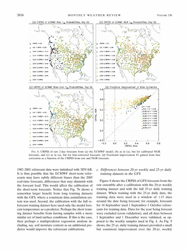
Figures 6a–c show the geographic distributions of day2 skill for the raw, NGR, and bias-corrected forecasts,respectively. The raw forecasts were commonly defi-cient in skill in the complex terrain of the westernUnited States and Canada, presumably because the

simplified terrain heights of the forecast model differedfrom that of the actual stations, with concomitant errorsin the estimation of surface temperatures. It appearedthat a simple bias correction achieved most of the im-pact for the stations with particularly unskillful rawforecasts. This is demonstrated in Fig. 6d. Here, thefractional improvement of the bias correction is plottedas a function of the raw and calibrated forecasts. Let-ting CRAW, CNGR, and CBC denote the CRPSS of theraw, calibrated, and bias-corrected forecasts, respec-tively, the fractional improvement Fr is computed as(CBC � CRAW)/(CNGR � CRAW). Figure 6d shows sev-eral interesting characteristics. First, note that the effectof the NGR calibration was primarily to improve fore-casts that started off as particularly unskillful by ho-mogenizing the resultant skill relative to the highlyvarying skills seen in the raw forecasts. Second, in gen-eral the locations that had relatively large improve-ments through the NGR calibration achieved a greaterfraction of this from the bias correction than did thelocations that had smaller improvements. Overall, the

FIG. 3. Average ensemble spread (with members additionally perturbed with randomsample of observation error drawn from R) and rmse of 2-m temperature forecasts from the(a) ECMWF and (b) GFS ensembles.

FIG. 4. CRPSS of surface temperature forecasts with andwithout calibration.


large improvements from bias corrections may indicatethat additional resolution may be helpful, leading tosmaller mismatches between model terrain height andstation elevation (see also Buizza et al. 2007).

b. Differences between 20-yr weekly and 30-daydaily training datasets

To facilitate a comparison of long and short trainingdatasets, the ECMWF and GFS ensemble forecastswere also extracted every day for the period 1 July–1December 2005. This permitted us to examine theefficacy of a smaller training dataset. Recent results(Stensrud and Yussouf 2005; Cui et al. 2006) have sug-gested that temperature forecast calibration may beable to be performed well even with a small number ofrecent forecasts. This may be because the ensembleforecast bias is relatively consistent and can be esti-mated with a small sample. Another possibility is thatrecent samples are more relevant for the statistical cor-rection, with their more similar circulation regimes andland surface states than data from other years.

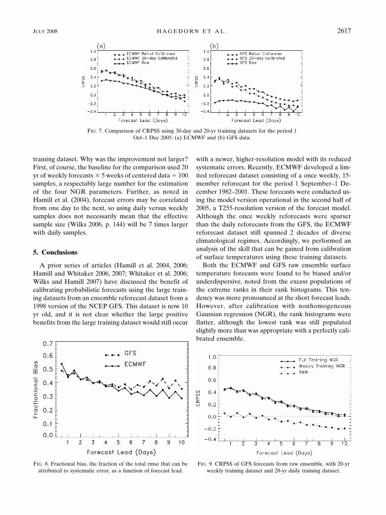
Accordingly, we compared the calibration of fore-casts using the prior 30 days as training data to calibra-tion using the full reforecast training dataset. Forecastswere compared for the period of 1 September–1 De-cember 2005. Nonhomogeneous Gaussian regressionwas again used for the calibration. Figure 7 shows thatat short forecast leads, the 30-day training dataset pro-vided approximately equal skill improvements relativeto the 20-yr training dataset for the ECMWF model,and marginally less for the GFS. However, as the fore-cast lead increased, then the benefit of the longer train-ing dataset became apparent.

Why were more samples particularly helpful for thelonger leads? We suggest that there were at least threecontributing factors. First, the prior 30-day trainingdataset was 9 days older for a 10-day forecast (trainingdays �39 to �10) than for a 1-day forecast (training

days �30 to �1). If errors were synoptically dependentand a regime change took place in the intervening 9days, the training set at 1-day lead will have hadsamples from the new regime but the training set at10-days lead will not. Second, determining the bias to aprespecified tolerance will require more samples atlong leads than at short leads. At these long leads, theproportion of the error attributable to bias shrinks be-cause of the rapid increase of errors due to chaoticerror growth. This is shown in Fig. 8; for the ECMWFmodel, this decreased from �0.54 at the half-day leadto �0.28 at the 10-day lead. Consequently, because theoverall error grows as the forecast lead increases and alarger proportion of it is attributable to random errors,determining the bias to a prespecified tolerance re-quires more samples. The third reason was that theshort-lead forecast training datasets were composed ofsamples that tended to have more independent errorsthan the longer-lead training datasets. The ECMWF1-day lagged correlation of forecast minus observedvalues averaged over all stations (not shown) increasedfrom around 0.2 at the early leads to 0.5 at the longerleads. Using the definition of an effective sample size n�(Wilks 2006, p. 144),

n� � n1 � �1

1 � �1, �10�

with n � 30, this indicates that the effective sample sizewas approximately 20 at the short leads and 10 at thelonger leads. The once weekly, 20-yr reforecast datasetshould, in comparison, be composed of samples that aretruly independent of each other.

Considering again the puzzling result of similar skillat short leads, we hypothesize that the two factors heremay have contributed to underestimating the poten-tial skill that can be obtained with a properly con-structed long training dataset. First, one limitation ofthe ECMWF datasets was that for the 2005 data,all forecasts were initialized with 4DVAR, but the

FIG. 5. CRPSS including bias-corrected ensemble forecasts for (a) ECMWF and (b) GFSforecasts.


1982–2001 reforecast data were initialized with 3DVAR.It is thus possible that the ECMWF short-term refor-ecasts may have subtly different biases than the 2005real-time forecasts, differences that may diminish withthe forecast lead. This would affect the calibration ofthe short-term forecasts. Notice that Fig. 7b shows asomewhat larger benefit from long training datasetswith the GFS, where a consistent data assimilation sys-tem was used. Second, the calibration with the full re-forecast training dataset here used only the model fore-cast temperature as a predictor. Perhaps the short train-ing dataset benefits from having samples with a moresimilar set of land surface conditions. If this is the case,then perhaps a multipredictor regression analysis in-cluding, say, soil moisture content as an additional pre-dictor would improve the reforecast calibrations.

c. Differences between 20-yr weekly and 25-yr dailytraining datasets in the GFS

Figure 9 shows the CRPSS of GFS forecasts from theraw ensemble after a calibration with the 20-yr weeklytraining dataset and with the full 25-yr daily trainingdataset. When training with the 25-yr daily data, thetraining data were used in a window of �15 daysaround the date being forecast; for example, forecastsfor 16 September used 1 September–1 October refore-casts for training data. Data for the year being forecastwere excluded (cross validation), and all days between1 September and 1 December were validated, as op-posed to the weekly samples used in Fig. 4. As Fig. 9shows, the 25-yr, daily training dataset provided a smallbut consistent improvement over the 20-yr, weekly

FIG. 6. CRPSS of raw 2-day forecasts from (a) the ECMWF model, (b) as in (a), but for calibrated NGRforecasts, and (c) as in (a), but for bias-corrected forecasts. (d) Fractional improvement Fr gained from biascorrection as a function of the CRPSS from raw and NGR forecasts.


Fig 6 live 4/C

training dataset. Why was the improvement not larger?First, of course, the baseline for the comparison used 20yr of weekly forecasts � 5 weeks of centered data � 100samples, a respectably large number for the estimationof the four NGR parameters. Further, as noted inHamill et al. (2004), forecast errors may be correlatedfrom one day to the next, so using daily versus weeklysamples does not necessarily mean that the effectivesample size (Wilks 2006, p. 144) will be 7 times largerwith daily samples.

5. Conclusions

A prior series of articles (Hamill et al. 2004, 2006;Hamill and Whitaker 2006, 2007; Whitaker et al. 2006;Wilks and Hamill 2007) have discussed the benefit ofcalibrating probabilistic forecasts using the large train-ing datasets from an ensemble reforecast dataset from a1998 version of the NCEP GFS. This dataset is now 10yr old, and it is not clear whether the large positivebenefits from the large training dataset would still occur

with a newer, higher-resolution model with its reducedsystematic errors. Recently, ECMWF developed a lim-ited reforecast dataset consisting of a once weekly, 15-member reforecast for the period 1 September–1 De-cember 1982–2001. These forecasts were conducted us-ing the model version operational in the second half of2005, a T255-resolution version of the forecast model.Although the once weekly reforecasts were sparserthan the daily reforecasts from the GFS, the ECMWFreforecast dataset still spanned 2 decades of diverseclimatological regimes. Accordingly, we performed ananalysis of the skill that can be gained from calibrationof surface temperatures using these training datasets.

Both the ECMWF and GFS raw ensemble surfacetemperature forecasts were found to be biased and/orunderdispersive, noted from the excess populations ofthe extreme ranks in their rank histograms. This ten-dency was more pronounced at the short forecast leads.However, after calibration with nonhomogeneousGaussian regression (NGR), the rank histograms wereflatter, although the lowest rank was still populatedslightly more than was appropriate with a perfectly cali-brated ensemble.

FIG. 8. Fractional bias, the fraction of the total rmse that can beattributed to systematic error, as a function of forecast lead.

FIG. 9. CRPSS of GFS forecasts from raw ensemble, with 20-yrweekly training dataset and 28-yr daily training dataset.

FIG. 7. Comparison of CRPSS using 30-day and 20-yr training datasets for the period 1Oct–1 Dec 2005: (a) ECMWF and (b) GFS data.


The skill of these forecasts was measured with amodified version of the continuous ranked probabilityskill score (CRPSS), with the computation adjusted toremove the tendency to award fictitious skill due tovariations in the forecast climatology (Hamill and Juras2006). Climatology provided the no-skill reference. Us-ing this skill measure, the raw GFS ensemble forecastshad near zero to negative skill at all leads due to thepresence of large forecast biases. The ECMWF rawforecasts retained positive skill to approximately 8days.

After calibration with NGR, the postprocessedGFS forecasts exceeded the skill of the uncalibratedECMWF forecasts at all leads. Here, the GFS trainingdata were subsampled to the same weekly, 20-yr set ofdates as in the ECMWF reforecast. However, the re-forecast-based, calibrated ECMWF forecasts weremuch more skillful than both the GFS calibrated fore-casts and the ECMWF uncalibrated forecasts, althoughthe absolute amount of skill increase from calibrationwas smaller for ECMWF than for the GFS. Nonethe-less, the ECMWF skill improvement was substantial;for example, the skill of a calibrated, 4–5-day ECMWFforecast was comparable to the skill of an uncalibrated1-day forecast. Approximately 70% of the improve-ment of the ECMWF could be attributed to a simplecorrection of mean bias in the forecasts, with a slightlysmaller percentage in the GFS. The ECMWF raw fore-casts were observed to have particularly low skill atstations in the intermountain western United States,perhaps due to larger discrepancies between the modelterrain and the station locations. Calibration was par-ticularly successful in increasing the skill at these sta-tions. Finally, a multimodel calibrated forecast wasmore skillful than either individual calibrated forecast.

The computation of an extensive reforecast dataset isexpensive, and a new reforecast dataset may be neededeach time a model change affects its systematic errorcharacteristics. If the same benefit could be achievedwith a much smaller set of recent forecasts, this wouldmake operational calibration much easier. Accordingly,using 2005 data, we compared the calibration using the1982–2001 reforecasts to calibration using the most re-cent 30 samples of forecasts from 2005. For the shorterforecast leads, the skill after calibration using thisshorter training dataset was very similar to thatachieved with large reforecast dataset. We hypothesizethat this benefit may be attributable to the more recentsamples being more similar in their error characteristicsthan those from the reforecast dataset, which samplesother years of data. However, at longer leads, the re-forecast dataset produced more skillful calibrated fore-

casts than the 30-day training dataset. This was likelydue to at least three reasons: first, 30 days of trainingdata for the longer-lead forecasts were more separatedfrom the actual forecast day of interest (e.g., when cali-brating a 10-day forecast, the most recent trainingsample is 10 days old because verification is not yetavailable for the more recent forecasts). Second, thenumber of samples necessary to estimate the bias to aprespecified tolerance generally increased with increas-ing forecast lead. And third, for forecasts at the longerleads, the samples on adjacent days tended to have cor-related forecast errors, thereby reducing the effectivesample size.

Although a daily reforecast dataset was yet not avail-able for the ECMWF model, the impact of daily versusweekly samples could be evaluated with the GFS re-forecast dataset. Using a 25-yr daily reforecast versus a20-yr weekly forecast produced a small but noticeableimprovement.

It is also possible that the calibration could be im-proved by including other predictors. Here we consid-ered only 2-m temperature as a predictor. Perhaps thereason the 30-day training dataset shows such good re-sults is that the training samples are from a regime withsimilar surface characteristics, such as soil moisture. Ifso, then the performance of a multiyear reforecastcould be enhanced by including soil moisture as an ad-ditional predictor. An examination of the potentialvalue of several other predictors may be useful beforeany operational implementation of a temperature-calibration scheme.

This article considered only the calibration of 2-mtemperature forecasts. Our experience with precipita-tion calibration using the GFS reforecasts suggests thatthe benefit from calibration using short trainingdatasets will be smaller than for temperature. The com-panion article to this paper (Hamill et al. 2008) exam-ines the calibration of ECMWF and GFS precipitationforecasts in more depth and provides substantial fur-ther evidence for the value of large training datasets,even with a state-of-the-art model. Nonetheless, thevalue of large training datasets for temperature calibra-tion was confirmed here, even for a current, state-of-the-art forecast model. Short training datasets were ad-equate for the short-lead forecasts, but to achieve ben-efits at all forecast leads, the longer training datasetproved useful.

Combined with the evidence in our companion paperand previous studies, there is now a growing body ofliterature indicating the potential utility of reforecastmethodology for improving operational ensemble pre-dictions.


Acknowledgments. Publication of this manuscriptwas supported by a NOAA THORPEX grant.

REFERENCES

Barkmeijer, J., M. van Gijzen, and F. Bouttier, 1998: Singularvectors and estimates of the analysis-error covariance metric.Quart. J. Roy. Meteor. Soc., 124, 1695–1713.

——, M. R. Buizza, and T. N. Palmer, 1999: 3D-Var Hessian sin-gular vectors and their potential use in the ECMWF en-semble prediction system. Quart. J. Roy. Meteor. Soc., 125,2333–2351.

Buizza, R., P. L. Houtekamer, Z. Toth, G. Pellerin, M. Wei, andY. Zhu, 2005: A comparison of the ECMWF, MSC, andNCEP global ensemble prediction systems. Mon. Wea. Rev.,133, 1076–1097.

——, J.-R. Bidlot, N. Wedi, M. Fuentes, M. Hamrud, G. Holt, andF. Vitart, 2007: The new ECMWF VAREPS (Variable Reso-lution Ensemble Prediction System). Quart. J. Roy. Meteor.Soc., 133, 681–695.

Casella, G., and R. L. Berger, 1990: Statistical Inference. Duxbury,650 pp.

Clark, M. P., and L. E. Hay, 2004: Use of medium-range weatherforecasts to produce predictions of streamflow. J. Hydrome-teor., 5, 15–32.

Cui, B., Z. Toth, Y. Zhu, D. Hou, D. Unger, and S. Beauregard,2006: The trade-off in bias correction between using the latestanalysis/modeling system with a short, versus an older systemwith a long archive. Proc. First THORPEX Int. ScienceSymp., Montréal, QC, Canada, World Meteorological Orga-nization, 281–284.

Daley, R., 1991: Atmospheric Data Analysis. Cambridge Univer-sity Press, 457 pp.

Eckel, F. A., and M. K. Walters, 1998: Calibrated probabilisticquantitative precipitation forecasts based on the MRF en-semble. Wea. Forecasting, 13, 1132–1147.

Gneiting, T., A. E. Raftery, A. H. Westveld III, and T. Goldman,2005: Calibrated probabilistic forecasting using ensemblemodel output statistics and minimum CRPS estimation. Mon.Wea. Rev., 133, 1098–1118.

Hamill, T. M., 1999: Hypothesis tests for evaluating numericalprecipitation forecasts. Wea. Forecasting, 14, 155–167.

——, 2001: Interpretation of rank histograms for verifying en-semble forecasts. Mon. Wea. Rev., 129, 550–560.

——, and S. J. Colucci, 1998: Evaluation of Eta–RSM ensembleprobabilistic precipitation forecasts. Mon. Wea. Rev., 126,711–724.

——, and J. Juras, 2006: Measuring forecast skill: Is it real skill oris it the varying climatology? Quart. J. Roy. Meteor. Soc., 132,2905–2923.

——, and J. S. Whitaker, 2006: Probabilistic quantitative precipi-tation forecasts based on reforecast analogs: Theory and ap-plication. Mon. Wea. Rev., 134, 3209–3229.

——, and ——, 2007: Ensemble calibration of 500-hPa geopoten-

tial height and 850-hPa and 2-m temperatures using refore-casts. Mon. Wea. Rev., 135, 3273–3280.

——, ——, and X. Wei, 2004: Ensemble reforecasting: Improvingmedium-range forecast skill using retrospective forecasts.Mon. Wea. Rev., 132, 1434–1447.

——, ——, and S. L. Mullen, 2006: Reforecasts: An importantdataset for improving weather predictions. Bull. Amer. Me-teor. Soc., 87, 33–46.

——, R. Hagedorn, and J. S. Whitaker, 2008: Probabilistic fore-cast calibration using ECMWF and GFS ensemble refore-casts. Part II: Precipitation. Mon. Wea. Rev., 136, 2620–2632.

Krishnamurti, T. N., C. M. Kishtawal, T. E. LaRow, D. R. Bachio-chi, Z. Zhang, C. E. Williford, S. Gadgil, and S. Surendran,1999: Improved weather and seasonal climate forecasts frommulti-model superensemble. Science, 285, 1548–1550.

Mahfouf, J.-F., and F. Rabier, 2000: The ECMWF operationalimplementation of four-dimensional variational assimilation.II: Experimental results with improved physics. Quart. J.Roy. Meteor. Soc., 126, 1171–1190.

Molteni, F., R. Buizza, T. N. Palmer, and T. Petroliagis, 1996: TheECMWF ensemble prediction system: Methodology and vali-dation. Quart. J. Roy. Meteor. Soc., 122, 73–119.

Parrish, D. F., and J. C. Derber, 1992: The National Meteorologi-cal Center’s spectral statistical-interpolation analysis system.Mon. Wea. Rev., 120, 1747–1763.

Raftery, A. E., T. Gneiting, F. Balabdaoui, and M. Polakowski,2005: Using Bayesian model averaging to calibrate forecastensembles. Mon. Wea. Rev., 133, 1155–1174.

Roulston, M. S., and L. A. Smith, 2003: Combining dynamical andstatistical ensembles. Tellus, 55A, 16–30.

Stensrud, D. J., and N. Yussouf, 2005: Bias-corrected short-rangeensemble forecasts of near surface variables. Meteor. Appl.,12, 217–230.

Uppala, S. M., and Coauthors, 2005: The ERA-40 re-analysis.Quart. J. Roy. Meteor. Soc., 131, 2961–3012.

Vislocky, R. L., and J. M. Fritsch, 1995: Improved model outputstatistics forecasts through model consensus. Bull. Amer. Me-teor. Soc., 76, 1157–1164.

——, and ——, 1997: Performance of an advanced MOS system inthe 1996-97 National Collegiate Weather Forecasting Con-test. Bull. Amer. Meteor. Soc., 78, 2851–2857.

Wang, X., and C. H. Bishop, 2005: Improvement of ensemble re-liability with a new dressing kernel. Quart. J. Roy. Meteor.Soc., 131, 965–986.

Whitaker, J. S., and A. F. Loughe, 1998: The relationship betweenensemble spread and ensemble mean skill. Mon. Wea. Rev.,126, 3292–3302.

——, X. Wei, and F. Vitart, 2006: Improving week-2 forecasts withmultimodel reforecast ensembles. Mon. Wea. Rev., 134, 2279–2284.

Wilks, D. S., 2006: Statistical Methods in the Atmospheric Sciences.2nd ed. Academic Press, 627 pp.

——, and T. M. Hamill, 2007: Comparison of ensemble-MOSmethods using GFS reforecasts. Mon. Wea. Rev., 135, 2379–2390.


probabilistic forecast calibration using ecmwf and gfs ...€¦ · probabilistic forecast...

Documents