probabilistic graphical models - cs.helsinki.fi · 2 christopher m. bishop nato asi: learning...

1

Probabilistic Graphical Models

Part Two: Inference and Learning

Christopher M. Bishop

Microsoft Research, Cambridge, U.K.

research.microsoft.com/~cmbishop

NATO ASI: Learning Theory and Practice, Leuven, July 2002

Christopher M. Bishop NATO ASI: Learning Theory and Practice, Leuven, July 2002

Overview of Part Two

• Exact inference and the junction tree

• MCMC

• Variational methods and EM

• Example• General variational inference engine




• MCMC




Exact Inference

• Group the hidden variables H into H1 and H2 in which we want to marginalize over H2 to find the posterior over H1

• Thus our most general inference problem involves evaluation of

• For a M-state discrete units there are terms in the summation where |H2 | is the number of hidden nodes

• Can easily become computationally intractable

• Can we exploit the conditional independence structure (missing links) to find more efficient algorithms?


Example

• Goal: find

• Direct evaluation gives

where, for variables having M states, the denominator involves summing over ML-1 terms (exponential in the length of the chain)


Example (cont’d)

• Using the conditional independence structure we can re-order the summations in the denominator to give

which involves summations (linear in the length of the chain) – similarly for the numerator

• Can be viewed as a local message passing algorithm

2


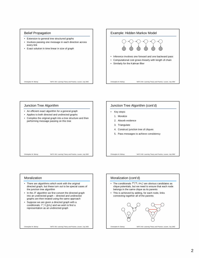
Belief Propagation

• Extension to general tree structured graphs

• Involves passing one message in each direction across every link

• Exact solution in time linear in size of graph


Example: Hidden Markov Model

• Inference involves one forward and one backward pass

• Computational cost grows linearly with length of chain• Similarly for the Kalman filter


Junction Tree Algorithm

• An efficient exact algorithm for a general graph

• Applies to both directed and undirected graphs

• Compiles the original graph into a tree structure and then performing message passing on this tree


Junction Tree Algorithm (cont’d)

• Key steps:

1. Moralize

2. Absorb evidence

3. Triangulate

4. Construct junction tree of cliques

5. Pass messages to achieve consistency


Moralization

• There are algorithms which work with the original directed graph, but these turn out to be special cases of the junction tree algorithm

• In the JT algorithm we first convert the directed graph into an undirected graph – directed and undirected graphs are then treated using the same approach

• Suppose we are given a directed graph with a conditionals and we wish to find a representation as an undirected graph


Moralization (cont’d)

• The conditionals are obvious candidates as clique potentials, but we need to ensure that each node belongs in the same clique as its parents

• This is achieved by adding, for each node, links connecting together all of the parents

3



• Moralization therefore consists of the following steps:

1. For each node in the graph, add an edge between all parents of the node and then convert directed edges to undirected edges

2. Initialize the clique potentials of the moral graph to 1

3. For each local conditional probability choose a clique C such that C contains both Xi and pai and multiply by

• Note that this undirected graph automatically has a normalization factor



• By adding links we have discarded some conditional independencies

• However, any conditional independencies in the moral graph also hold for the original directed graph, so if we solve the inference problem for the moral graph we will solve it also for the directed graph


Absorbing Evidence

• The nodes can be grouped into visible V for, which we have particular observed values , and hidden H

• We are interested in the conditional (posterior) probability

• Absorb evidence simply by altering the clique potentials to be zero for any configuration inconsistent with


Absorbing Evidence (cont’d)

• We can view

as an un-normalized version of

and hence an un-normalized version of


Local Consistency

• As it stands, the graph correctly represents the (un-normalized) joint distribution but the clique potentials do not have an interpretation as marginal probabilities

• Our goal is to update the clique potentials so that they acquire a local probabilistic interpretation while preserving the global distribution


Local Consistency (cont’d)

• Note that we cannot simply have

with

as can be seen by considering the three node graph

• Here

4



• Instead we consider the more general representation for undirected graphs including separator sets, then we have



• Starting from our un-normalized representation of in terms of products of clique potentials,

we can introduce separator potentials initially set to unity

Note that nodes can appear in more than one clique, and we require that these be consistent for all marginals

• Achieving consistency is central to the junction tree algorithm



• Consider the elemental problem of achieving consistency between a pair of cliques V and W, with separator set S

• Initially



• First construct a “message” at clique V and pass to W

• Since is unchanged , and so the joint distribution is invariant



• Next pass a message back from W to V using the same update rule

• Here is unchanged and so , and again the joint distribution is unchanged

• The marginals are now correct for both of the cliques and also for the separator



• Example: return to the earlier three node graph

• Initially the clique potentials are and , and the separator potential

• The first message pass gives the following update

which are the correct marginals• In this case the second message is vacuous

5



• Now suppose that node A is observed (for simplicity consider nodes to be binary and suppose A=1)

• Absorbing the evidence involves altering the potential by setting the A=0 row to zero

• Summing over A gives

• Updating the potential gives



• Hence the potentials after the first message pass are

• Again the reverse message is vacuous

• Note that the resulting clique and separator marginals require normalization (a local operation)


Global Consistency

• How can we extend our two-clique procedure to ensure consistency across the whole graph?

• We construct a clique tree by considering a spanning tree linking all of the cliques which is maximal with respect to the cardinality of the intersection sets

• Next we construct and pass messages using the following protocol:

– a clique can send a message to a neighbouring clique only when it has received messages from all of its neighbours


Global Consistency (cont’d)

• In practice this can be achieved by designating one clique as root and then

– (i) collecting evidence by passing messages from the leaves to the root

– (ii) distributing evidence by propagating outwards from the root to the leaves


One Last Issue

• The algorithm discussed so far is not quite sufficient to guarantee consistency for an arbitrary graph

• Consider the four node graph here, together with a maximal spanning clique tree

• Node C appears in two places and there is no guarantee that local consistency for P(C) will result in global consistency


One Last Issue (cont’d)

• The problem is resolved if the tree of cliques is a junction tree, i.e. if for every pair of cliques V and W all cliques on the (unique) path from V to W contain V W (running intersection property)

• As a by-product we are also guaranteed that the (now consistent) clique potentials are indeed marginals

6


One Last Issue (cont’d)

• How do we ensure that the maximal spanning tree of cliques will be a junction tree?

• Result: a graph has a junction tree if, and only if, it is triangulated, i.e. there are no chordless cycles of four or more nodes in the graph

• Example of a graph and its triangulated counterpart


Summary of Junction Tree Algorithm

• Key steps:

1.Moralize

2.Absorb evidence

3.Triangulate

4.Construct junction tree

5.Pass messages to achieve consistency


Example of JT Algorithm

• Original directed graph


Example of JT Algorithm (cont’d)

• Moralization



• Undirected graph



• Triangulation

7



• Junction tree


Limitations of Exact Inference

• The computational cost of the junction tree algorithm is determined by the size of the largest clique

• For densely connected graphs exact inference may be intractable

• There are 3 widely used approximation schemes

– Pretend graph is a tree: “loopy belief propagation”

– Markov chain Monte Carlo (e.g. Gibbs sampling)

– Variational inference




• MCMC

• EM algorithm

• Variational methods• Example

• General variational inference engine


MCMC

• Eventual goal is to evaluate averages of functions

where is typically the posterior distribution of (somesubset of) the hidden variables


MCMC (cont’d)

• Sampling methods aim to draw a sample of K points from the distribution and then to approximate the expectation by a finite sum

• This has the correct mean and variance

which is independent of dimensionality

• We can achieve excellent accuracy for small values of K

• However, this assumes sample points are independent!


MCMC (cont’d)

• Gibbs sampling samples each variable in turn using its conditional distribution conditioned on the other variables

• Not limited to conjugate-exponential distributions

• For graphical models, these conditional distributions depend only on the variables in the Markov blanket

• Software implementation: BUGS (Spiegelhalter et al.)

8


MCMC (cont’d)

• The problem with Gibbs sampling is that successive points are highly correlated

• In this example it takes of order steps to generate independent samples (random walk)

X1

X2

L

l




• MCMC




Learning in Graphical Models

• Introduce parameters which govern the

conditional distributions in a directed graph,

or clique potentials in an undirected graph

• Maximum likelihood: determine by

• Problem: the summation over H inside the logarithm may be intractable


Expectation-maximization (EM) Algorithm

• E-step: evaluate the posterior distribution using current estimate for the parameters

• M-step: re-estimate by maximizing the expected complete-data log likelihood

• Note that the log and the summation have been exchanged – this will often make the summation tractable

• Iterate E and M steps until convergence


EM Example: Mixtures of Gaussians


EM Example: Mixtures of Gaussians (cont’d)

9












EM: Variational Viewpoint

• For an arbitrary distribution we have

where

• Kullback-Leibler divergence satisfies with equality if and only if

• Hence is a rigorous lower bound on the log marginal likelihood

10


EM: Variational Viewpoint (cont’d)

ln ( )P V |θ�

( , )Q θ

KL( || )Q P



• If we maximize with respect to a free-form Q distribution we obtain

which is the true posterior distribution

• The lower bound then becomes

which, as a function of is the expected complete-data log likelihood (up to an additive constant)



ln ( )P V |θ ln ( )P V |θ ln ( )P V |θ

KL( || )Q P

KL

�( , )Q θ

�( , )Q θ�

( , )Q θ


Generalizations of EM

• What if the M-step is intractable?

– Use non-linear optimization to increase w.r.t.

• What if the E-step is intractable?

– Perform a partial optimization of w.r.t. Q– e.g. define a parametric family

– An alternative approach will be discussed later


Variational EM

ln ( )P V |θ ln ( )P V |θ ln ( )P V |θ

KL( || )Q P KL

�( , )Q θ

�( , )Q θ

�( , )Q θ


Bayesian Learning

• Introduce prior distributions over parameters

• Equivalent to graph with additional hidden variables

• Learning becomes inference on the expanded graph

• No distinction between variables and parameters• No M-step, just an E-step

• Example: mixture of Gaussians

11


Variational Inference

• We have already seen that the posterior distribution may be approximated by maximizing a lower bound

• For a suitable choice of this summation may be tractable even though

is not


Variational Inference (cont’d)

• The goal is to choose a sufficiently simple family of distributions that can be evaluated

• However, the family should also be sufficiently rich that a good approximation to the true posterior can be obtained

• One possibility is to use a parametric family of distributions



• Here we consider an alternative approach based on the assumption that factorizes with respect to subsets of nodes

where we leave the conditioning on V implicit

• Substituting into and dissecting out the contribution from we obtain



• We recognize this as the negative KL divergence between and an effective distribution given by

• Hence if we perform a free-form optimization over we obtain



• This is an implicit solution which depends on all

• Hence we initialize the factors and then cyclically update to convergence

• For conjugate-exponential choices of the conditional distributions in the directed graph, the solutions for will have closed form




• MCMC



12


Examples of Variational Inference

• Hidden Markov models (MacKay)

• Neural networks (Hinton)

• Bayesian PCA (Bishop)

• Independent Component Analysis (Attias)• Mixtures of Gaussians (Attias; Ghahramani and Beal)

• Mixtures of Bayesian PCA (Bishop and Winn)

• Flexible video sprites (Frey et al.)

• Audio-video fusion for tracking (Attias et al.)

• Latent Dirichlet Allocation (Jordan et al.)

• Relevance Vector Machine (Bishop and Tipping)

• …


Illustration: Relevance Vector Machine (RVM)

• Limitations of the support vector machine (SVM):

– Two classes

– Large number of kernels (in spite of sparsity)

– Kernels must satisfy Mercer criterion– Cross-validation to set parameters C (and � )

– Decisions at outputs instead of probabilities


Illustration: RVM (cont’d)

• The Relevance Vector Machine (Tipping, 1999) is a probabilistic regression or classification model

• Alternative to SVM, not a Bayesian interpretation of SVM• Properties

– Comparable error rates to SVM on new data– Comparable training speeds– No cross-validation to set parameters C (and � )– Applicable to wide choice of basis function– Multi-class classification– Probabilistic outputs– Dramatically fewer kernels

• Original RVM based on type II maximum likelihood –here we consider a variational treatment



• Linear model as for SVM

• Input vectors and targets

• Regression

• Likelihood function



• Gaussian prior for with hyper-parameters

• Gamma hyper-priors over and



• Graphical model representation

13



• Variational posterior distribution

• Analytical solutions for optimum factors



• Sufficient statistics given by



• Moments given by

where the di-gamma function is defined by



• A high proportion of are driven to large values in the posterior distribution, giving a sparse modelLower bound can also be evaluated explicitly

• Variational treatment can be extended to classification



• Synthetic data: noisy sinusoid

-10 -5 0 5 10

-0.2

0

0.2

0.4

0.6

0.8

1 TruthVRVM



-2 0 2 40

5

10

15

20

log10

�α �

0 20 40

-1

0

1

2

mea

n w

eigh

t val

ue

• Synthetic data: noisy sinusoid

14


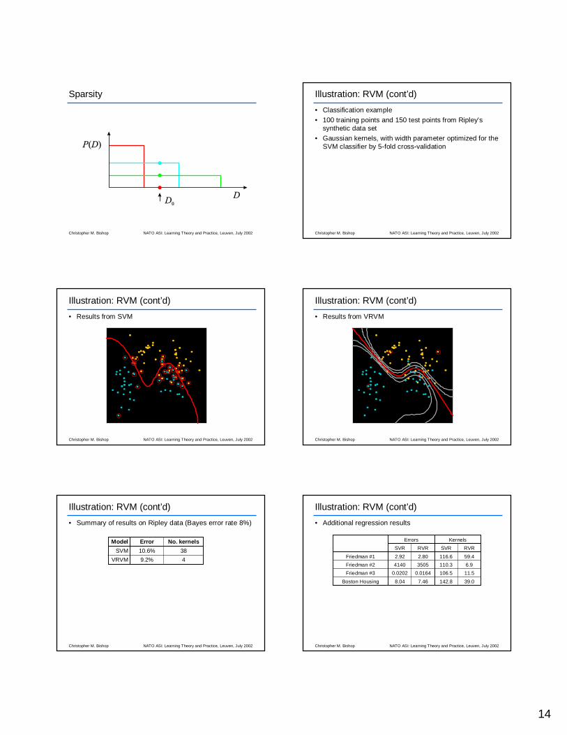
Sparsity

DD0

P D( )



• Classification example

• 100 training points and 150 test points from Ripley's synthetic data set

• Gaussian kernels, with width parameter optimized for the SVM classifier by 5-fold cross-validation



• Results from SVM



• Results from VRVM



• Summary of results on Ripley data (Bayes error rate 8%)

49.2%VRVM

3810.6%SVM

No. kernelsErrorModel



• Additional regression results

39.0142.87.468.04Boston Housing

11.5106.50.01640.0202Friedman #3

6.9110.335054140Friedman #2

59.4116.62.802.92Friedman #1

RVRSVRRVRSVR

KernelsErrors

15



• Additional classification results

5.1%

65

RVM

2540

109

SVM

316--4.4%U.S.P.S.

42006867Pima Indians

RVMGPGPSVM

KernelsErrors




• MCMC




General Variational Framework

• Currently for each new model we have to derive the variational update equations and then subsequently we write application-specific code to find the solution

• Can we build a general-purpose inference engine which automates these procedures?


VIBES

• Variational Inference for Bayesian Networks

• Bishop, Spiegelhalter and Winn (1999)

• A general inference engine using variational methods

• VIBES will be made available on the WWW


VIBES (cont’d)

• A key observation is that in the general solution

the update for a particular node (or group of nodes) depends only on other nodes in the Markov blanket

• Permits a local object-oriented implementation which is independent of the particular graph structure


VIBES (cont’d)

16


VIBES (cont’d)


VIBES (cont’d)


Summary of Part Two

• Exact inference algorithms can be formulated in terms of graphical manipulations (the junction tree)

• Bayesian learning is just inference on an expanded graph

• Variational methods provide a powerful semi-analytical tool for approximate inference in graphical models


Bibliography• Probabilistic Networks and Expert Systems. R. G. Cowell, A. P. Dawid, S. L.

Lauritzen and D. J. Spiegelhalter (1999). Springer.• Graphical Models. S. L. Lauritzen. Oxford University Press.

• Learning in Graphical Models. M. I. Jordan, Ed (1998). MIT Press.

• Graphical Models for Machine Learning and Digital Communication. B. J. Frey (1998). MIT Press.

• Tutorial on Variational Approximation Methods. T. S. Jaakkola, MIT.

• Variational Relevance Vector Machines. C. M. Bishop and M. E. Tipping (2000). In Proc. 16th Conference on Uncertainty in Artificial Intelligence (UAI). Ed. C. Boutilier and M. Goldszmidt, Morgan Kaufmann, 46–53.

• Propagation algorithms for variational Bayesian learning. Z. Ghahramani, and

M. J. Beal (2001). Neural Information Processing Systems 13, MIT Press.

Viewgraphs and tutorials available from:

research.microsoft.com/~cmbishop

probabilistic graphical models - cs.helsinki.fi · 2 christopher m. bishop nato asi: learning...

Documents