probabilistic graphical models part i: bayesian belief...
TRANSCRIPT
Probabilistic Graphical ModelsPart I: Bayesian Belief Networks
Selim Aksoy
Department of Computer EngineeringBilkent University
CS 551, Fall 2018
CS 551, Fall 2018 c©2018, Selim Aksoy (Bilkent University) 1 / 27
Introduction
I Graphs are an intuitive way of representing and visualizingthe relationships among many variables.
I Probabilistic graphical models provide a tool to deal withtwo problems: uncertainty and complexity.
I Hence, they provide a compact representation of jointprobability distributions using a combination of graph theoryand probability theory.
I The graph structure specifies statistical dependenciesamong the variables and the local probabilistic modelsspecify how these variables are combined.
CS 551, Fall 2018 c©2018, Selim Aksoy (Bilkent University) 2 / 27
Introduction
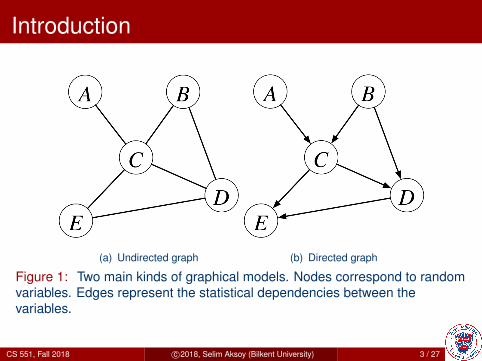
(a) Undirected graph (b) Directed graph
Figure 1: Two main kinds of graphical models. Nodes correspond to randomvariables. Edges represent the statistical dependencies between thevariables.
CS 551, Fall 2018 c©2018, Selim Aksoy (Bilkent University) 3 / 27

Introduction
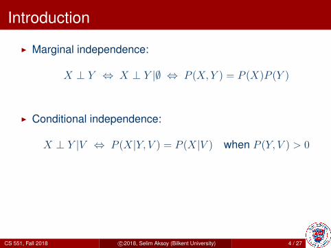
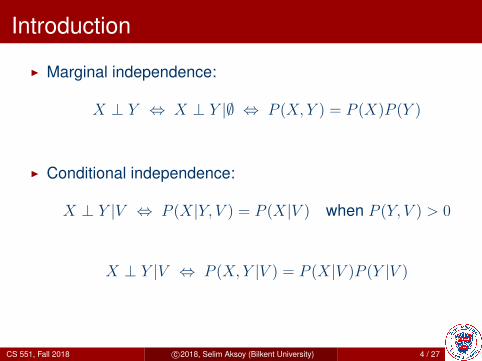
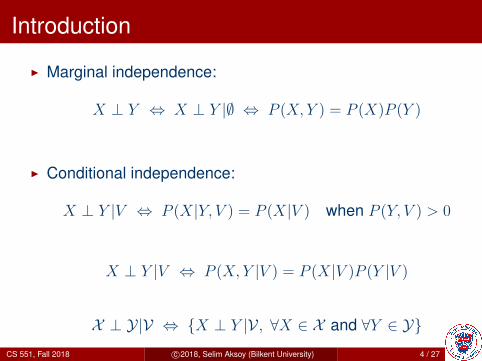
I Marginal independence:
X ⊥ Y ⇔ X ⊥ Y |∅ ⇔ P (X, Y ) = P (X)P (Y )
I Conditional independence:
X ⊥ Y |V ⇔ P (X|Y, V ) = P (X|V ) when P (Y, V ) > 0
X ⊥ Y |V ⇔ P (X, Y |V ) = P (X|V )P (Y |V )
X ⊥ Y|V ⇔ {X ⊥ Y |V , ∀X ∈ X and ∀Y ∈ Y}
CS 551, Fall 2018 c©2018, Selim Aksoy (Bilkent University) 4 / 27
Introduction
I Marginal independence:
X ⊥ Y ⇔ X ⊥ Y |∅ ⇔ P (X, Y ) = P (X)P (Y )
I Conditional independence:
X ⊥ Y |V ⇔ P (X|Y, V ) = P (X|V ) when P (Y, V ) > 0
X ⊥ Y |V ⇔ P (X, Y |V ) = P (X|V )P (Y |V )
X ⊥ Y|V ⇔ {X ⊥ Y |V , ∀X ∈ X and ∀Y ∈ Y}CS 551, Fall 2018 c©2018, Selim Aksoy (Bilkent University) 4 / 27

Introduction
I Marginal and conditional independence examples:I Amount of speeding fine ⊥ Type of car | Speed
I Lung cancer ⊥ Yellow teeth | SmokingI (Position,Velocity)t+1 ⊥
(Position,Velocity)t−1 | (Position,Velocity)t,Accelerationt
I Child’s genes ⊥ Grandparents’ genes | Parents’ genesI Ability of team A ⊥ Ability of team BI not(Ability of team A ⊥
Ability of team B | Outcome of A vs B game)
CS 551, Fall 2018 c©2018, Selim Aksoy (Bilkent University) 5 / 27

Introduction
I Marginal and conditional independence examples:I Amount of speeding fine ⊥ Type of car | SpeedI Lung cancer ⊥ Yellow teeth | Smoking
I (Position,Velocity)t+1 ⊥(Position,Velocity)t−1 | (Position,Velocity)t,Accelerationt
I Child’s genes ⊥ Grandparents’ genes | Parents’ genesI Ability of team A ⊥ Ability of team BI not(Ability of team A ⊥
Ability of team B | Outcome of A vs B game)
CS 551, Fall 2018 c©2018, Selim Aksoy (Bilkent University) 5 / 27

Introduction
I Marginal and conditional independence examples:I Amount of speeding fine ⊥ Type of car | SpeedI Lung cancer ⊥ Yellow teeth | SmokingI (Position,Velocity)t+1 ⊥
(Position,Velocity)t−1 | (Position,Velocity)t,Accelerationt
I Child’s genes ⊥ Grandparents’ genes | Parents’ genesI Ability of team A ⊥ Ability of team BI not(Ability of team A ⊥
Ability of team B | Outcome of A vs B game)
CS 551, Fall 2018 c©2018, Selim Aksoy (Bilkent University) 5 / 27

Introduction
I Marginal and conditional independence examples:I Amount of speeding fine ⊥ Type of car | SpeedI Lung cancer ⊥ Yellow teeth | SmokingI (Position,Velocity)t+1 ⊥
(Position,Velocity)t−1 | (Position,Velocity)t,Accelerationt
I Child’s genes ⊥ Grandparents’ genes | Parents’ genes
I Ability of team A ⊥ Ability of team BI not(Ability of team A ⊥
Ability of team B | Outcome of A vs B game)
CS 551, Fall 2018 c©2018, Selim Aksoy (Bilkent University) 5 / 27

Introduction
I Marginal and conditional independence examples:I Amount of speeding fine ⊥ Type of car | SpeedI Lung cancer ⊥ Yellow teeth | SmokingI (Position,Velocity)t+1 ⊥
(Position,Velocity)t−1 | (Position,Velocity)t,Accelerationt
I Child’s genes ⊥ Grandparents’ genes | Parents’ genesI Ability of team A ⊥ Ability of team B
I not(Ability of team A ⊥Ability of team B | Outcome of A vs B game)
CS 551, Fall 2018 c©2018, Selim Aksoy (Bilkent University) 5 / 27

Introduction
I Marginal and conditional independence examples:I Amount of speeding fine ⊥ Type of car | SpeedI Lung cancer ⊥ Yellow teeth | SmokingI (Position,Velocity)t+1 ⊥
(Position,Velocity)t−1 | (Position,Velocity)t,Accelerationt
I Child’s genes ⊥ Grandparents’ genes | Parents’ genesI Ability of team A ⊥ Ability of team BI not(Ability of team A ⊥
Ability of team B | Outcome of A vs B game)
CS 551, Fall 2018 c©2018, Selim Aksoy (Bilkent University) 5 / 27
Bayesian Networks
I Bayesian networks (BN) are probabilistic graphical modelsthat are based on directed acyclic graphs.
I There are two components of a BN model: M = {G,Θ}.I Each node in the graph G represents a random variable and
edges represent conditional independence relationships.I The set Θ of parameters specifies the probability
distributions associated with each variable.
CS 551, Fall 2018 c©2018, Selim Aksoy (Bilkent University) 6 / 27
Bayesian Networks
I Bayesian networks (BN) are probabilistic graphical modelsthat are based on directed acyclic graphs.
I There are two components of a BN model: M = {G,Θ}.
I Each node in the graph G represents a random variable andedges represent conditional independence relationships.
I The set Θ of parameters specifies the probabilitydistributions associated with each variable.
CS 551, Fall 2018 c©2018, Selim Aksoy (Bilkent University) 6 / 27
Bayesian Networks
I Bayesian networks (BN) are probabilistic graphical modelsthat are based on directed acyclic graphs.
I There are two components of a BN model: M = {G,Θ}.I Each node in the graph G represents a random variable and
edges represent conditional independence relationships.
I The set Θ of parameters specifies the probabilitydistributions associated with each variable.
CS 551, Fall 2018 c©2018, Selim Aksoy (Bilkent University) 6 / 27

Bayesian Networks
I Bayesian networks (BN) are probabilistic graphical modelsthat are based on directed acyclic graphs.
I There are two components of a BN model: M = {G,Θ}.I Each node in the graph G represents a random variable and
edges represent conditional independence relationships.I The set Θ of parameters specifies the probability
distributions associated with each variable.
CS 551, Fall 2018 c©2018, Selim Aksoy (Bilkent University) 6 / 27
Bayesian Networks
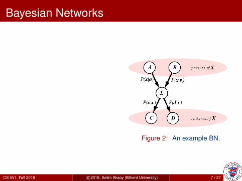
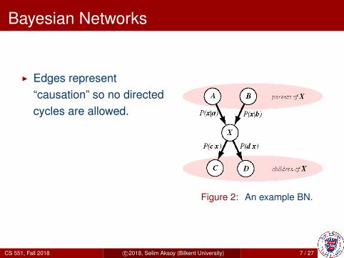
I Edges represent“causation” so no directedcycles are allowed.
I Markov property: Eachnode is conditionallyindependent of itsancestors given its parents.
Figure 2: An example BN.
CS 551, Fall 2018 c©2018, Selim Aksoy (Bilkent University) 7 / 27
Bayesian Networks
I Edges represent“causation” so no directedcycles are allowed.
I Markov property: Eachnode is conditionallyindependent of itsancestors given its parents.
Figure 2: An example BN.
CS 551, Fall 2018 c©2018, Selim Aksoy (Bilkent University) 7 / 27

Bayesian Networks
I Edges represent“causation” so no directedcycles are allowed.
I Markov property: Eachnode is conditionallyindependent of itsancestors given its parents.
Figure 2: An example BN.
CS 551, Fall 2018 c©2018, Selim Aksoy (Bilkent University) 7 / 27
Bayesian Networks
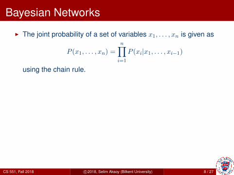
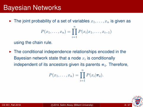
I The joint probability of a set of variables x1, . . . , xn is given as
P (x1, . . . , xn) =
n∏i=1
P (xi|x1, . . . , xi−1)
using the chain rule.
I The conditional independence relationships encoded in theBayesian network state that a node xi is conditionallyindependent of its ancestors given its parents πi. Therefore,
P (x1, . . . , xn) =n∏
i=1
P (xi|πi).
I Once we know the joint probability distribution encoded in thenetwork, we can answer all possible inference questions aboutthe variables using marginalization.
CS 551, Fall 2018 c©2018, Selim Aksoy (Bilkent University) 8 / 27
Bayesian Networks
I The joint probability of a set of variables x1, . . . , xn is given as
P (x1, . . . , xn) =
n∏i=1
P (xi|x1, . . . , xi−1)
using the chain rule.
I The conditional independence relationships encoded in theBayesian network state that a node xi is conditionallyindependent of its ancestors given its parents πi. Therefore,
P (x1, . . . , xn) =
n∏i=1
P (xi|πi).
I Once we know the joint probability distribution encoded in thenetwork, we can answer all possible inference questions aboutthe variables using marginalization.
CS 551, Fall 2018 c©2018, Selim Aksoy (Bilkent University) 8 / 27
Bayesian Network Examples
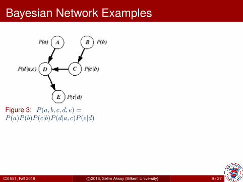
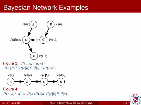
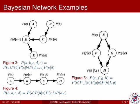
Figure 3: P (a, b, c, d, e) =P (a)P (b)P (c|b)P (d|a, c)P (e|d)
Figure 4:P (a, b, c, d) = P (a)P (b|a)P (c|b)P (d|c)
Figure 5: P (e, f, g, h) =P (e)P (f |e)P (g|e)P (h|f, g)
CS 551, Fall 2018 c©2018, Selim Aksoy (Bilkent University) 9 / 27
Bayesian Network Examples
Figure 3: P (a, b, c, d, e) =P (a)P (b)P (c|b)P (d|a, c)P (e|d)
Figure 4:P (a, b, c, d) = P (a)P (b|a)P (c|b)P (d|c)
Figure 5: P (e, f, g, h) =P (e)P (f |e)P (g|e)P (h|f, g)
CS 551, Fall 2018 c©2018, Selim Aksoy (Bilkent University) 9 / 27
Bayesian Network Examples
Figure 3: P (a, b, c, d, e) =P (a)P (b)P (c|b)P (d|a, c)P (e|d)
Figure 4:P (a, b, c, d) = P (a)P (b|a)P (c|b)P (d|c)
Figure 5: P (e, f, g, h) =P (e)P (f |e)P (g|e)P (h|f, g)
CS 551, Fall 2018 c©2018, Selim Aksoy (Bilkent University) 9 / 27
Bayesian Network Examples
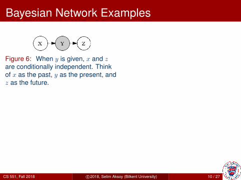
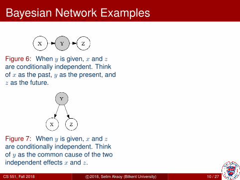
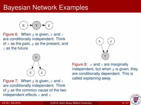
Figure 6: When y is given, x and zare conditionally independent. Thinkof x as the past, y as the present, andz as the future.
Figure 7: When y is given, x and zare conditionally independent. Thinkof y as the common cause of the twoindependent effects x and z.
Figure 8: x and z are marginallyindependent, but when y is given, theyare conditionally dependent. This iscalled explaining away.
CS 551, Fall 2018 c©2018, Selim Aksoy (Bilkent University) 10 / 27
Bayesian Network Examples
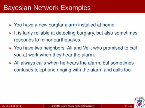
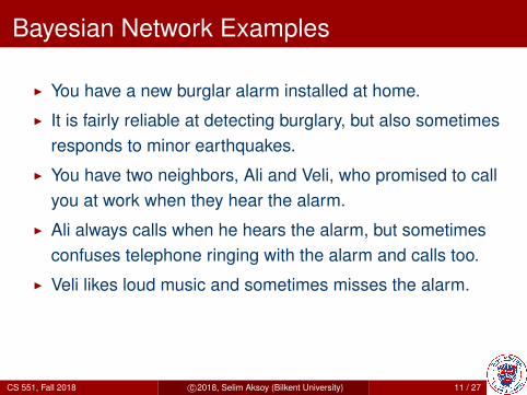
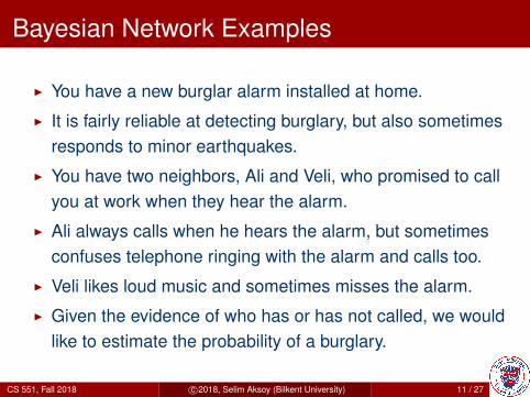
I You have a new burglar alarm installed at home.
I It is fairly reliable at detecting burglary, but also sometimesresponds to minor earthquakes.
I You have two neighbors, Ali and Veli, who promised to callyou at work when they hear the alarm.
I Ali always calls when he hears the alarm, but sometimesconfuses telephone ringing with the alarm and calls too.
I Veli likes loud music and sometimes misses the alarm.
I Given the evidence of who has or has not called, we wouldlike to estimate the probability of a burglary.
CS 551, Fall 2018 c©2018, Selim Aksoy (Bilkent University) 11 / 27
Bayesian Network Examples
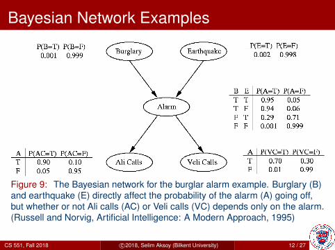
Figure 9: The Bayesian network for the burglar alarm example. Burglary (B)and earthquake (E) directly affect the probability of the alarm (A) going off,but whether or not Ali calls (AC) or Veli calls (VC) depends only on the alarm.(Russell and Norvig, Artificial Intelligence: A Modern Approach, 1995)
CS 551, Fall 2018 c©2018, Selim Aksoy (Bilkent University) 12 / 27
Bayesian Network Examples
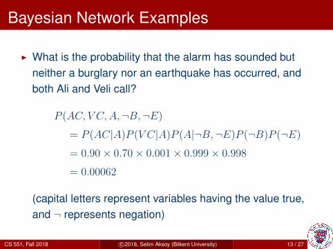
I What is the probability that the alarm has sounded butneither a burglary nor an earthquake has occurred, andboth Ali and Veli call?
P (AC, V C,A,¬B,¬E)= P (AC|A)P (V C|A)P (A|¬B,¬E)P (¬B)P (¬E)= 0.90× 0.70× 0.001× 0.999× 0.998
= 0.00062
(capital letters represent variables having the value true,and ¬ represents negation)
CS 551, Fall 2018 c©2018, Selim Aksoy (Bilkent University) 13 / 27
Bayesian Network Examples
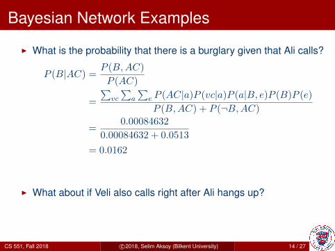
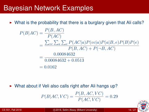
I What is the probability that there is a burglary given that Ali calls?
P (B|AC) =P (B,AC)
P (AC)
=
∑vc
∑a
∑e P (AC|a)P (vc|a)P (a|B, e)P (B)P (e)
P (B,AC) + P (¬B,AC)
=0.00084632
0.00084632 + 0.0513
= 0.0162
I What about if Veli also calls right after Ali hangs up?
P (B|AC, V C) =P (B,AC, V C)
P (AC, V C)= 0.29
CS 551, Fall 2018 c©2018, Selim Aksoy (Bilkent University) 14 / 27

Bayesian Network Examples
I What is the probability that there is a burglary given that Ali calls?
P (B|AC) =P (B,AC)
P (AC)
=
∑vc
∑a
∑e P (AC|a)P (vc|a)P (a|B, e)P (B)P (e)
P (B,AC) + P (¬B,AC)
=0.00084632
0.00084632 + 0.0513
= 0.0162
I What about if Veli also calls right after Ali hangs up?
P (B|AC, V C) =P (B,AC, V C)
P (AC, V C)= 0.29
CS 551, Fall 2018 c©2018, Selim Aksoy (Bilkent University) 14 / 27
Bayesian Network Examples
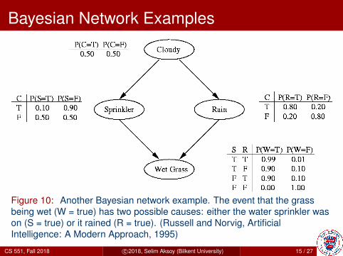
Figure 10: Another Bayesian network example. The event that the grassbeing wet (W = true) has two possible causes: either the water sprinkler wason (S = true) or it rained (R = true). (Russell and Norvig, ArtificialIntelligence: A Modern Approach, 1995)
CS 551, Fall 2018 c©2018, Selim Aksoy (Bilkent University) 15 / 27
Bayesian Network Examples
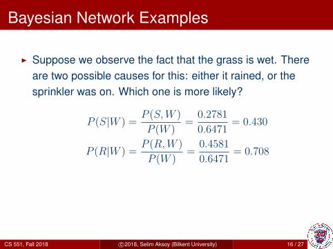
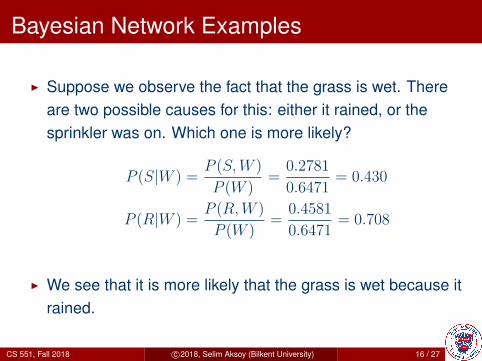
I Suppose we observe the fact that the grass is wet. Thereare two possible causes for this: either it rained, or thesprinkler was on. Which one is more likely?
P (S|W ) =P (S,W )
P (W )=
0.2781
0.6471= 0.430
P (R|W ) =P (R,W )
P (W )=
0.4581
0.6471= 0.708
I We see that it is more likely that the grass is wet because itrained.
CS 551, Fall 2018 c©2018, Selim Aksoy (Bilkent University) 16 / 27
Bayesian Network Examples
I Suppose we observe the fact that the grass is wet. Thereare two possible causes for this: either it rained, or thesprinkler was on. Which one is more likely?
P (S|W ) =P (S,W )
P (W )=
0.2781
0.6471= 0.430
P (R|W ) =P (R,W )
P (W )=
0.4581
0.6471= 0.708
I We see that it is more likely that the grass is wet because itrained.
CS 551, Fall 2018 c©2018, Selim Aksoy (Bilkent University) 16 / 27

Applications of Bayesian Networks
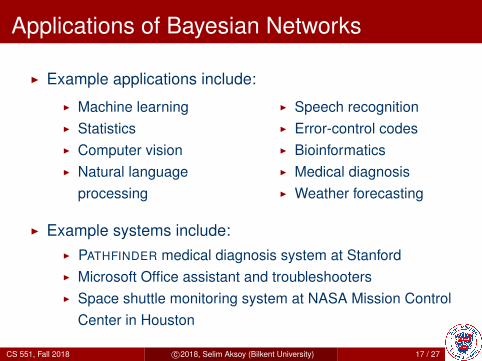
I Example applications include:
I Machine learningI StatisticsI Computer visionI Natural language
processing
I Speech recognitionI Error-control codesI BioinformaticsI Medical diagnosisI Weather forecasting
I Example systems include:I PATHFINDER medical diagnosis system at StanfordI Microsoft Office assistant and troubleshootersI Space shuttle monitoring system at NASA Mission Control
Center in Houston
CS 551, Fall 2018 c©2018, Selim Aksoy (Bilkent University) 17 / 27
Applications of Bayesian Networks
I Example applications include:
I Machine learningI StatisticsI Computer visionI Natural language
processing
I Speech recognitionI Error-control codesI BioinformaticsI Medical diagnosisI Weather forecasting
I Example systems include:I PATHFINDER medical diagnosis system at StanfordI Microsoft Office assistant and troubleshootersI Space shuttle monitoring system at NASA Mission Control
Center in Houston
CS 551, Fall 2018 c©2018, Selim Aksoy (Bilkent University) 17 / 27

Two Fundamental Problems for BNs
I Evaluation (inference) problem: Given the model and thevalues of the observed variables, estimate the values of thehidden nodes.
I Learning problem: Given training data and prior information(e.g., expert knowledge, causal relationships), estimate thenetwork structure, or the parameters of the probabilitydistributions, or both.
CS 551, Fall 2018 c©2018, Selim Aksoy (Bilkent University) 18 / 27
Bayesian Network Evaluation Problem
I If we observe the “leaves” and try to infer the values of thehidden causes, this is called diagnosis, or bottom-upreasoning.
I If we observe the “roots” and try to predict the effects, this iscalled prediction, or top-down reasoning.
I Exact inference is an NP-hard problem because thenumber of terms in the summations (integrals) for discrete(continuous) variables grows exponentially with increasingnumber of variables.
CS 551, Fall 2018 c©2018, Selim Aksoy (Bilkent University) 19 / 27
Bayesian Network Evaluation Problem
I Some restricted classes of networks, namely the singlyconnected networks where there is no more than one pathbetween any two nodes, can be efficiently solved in timelinear in the number of nodes.
I There are also clustering algorithms that convert multiplyconnected networks to single connected ones.
I However, approximate inference methods such asI sampling (Monte Carlo) methodsI variational methodsI loopy belief propagation
have to be used for most of the cases.
CS 551, Fall 2018 c©2018, Selim Aksoy (Bilkent University) 20 / 27
Bayesian Network Learning Problem
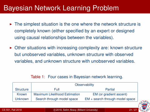
I The simplest situation is the one where the network structure iscompletely known (either specified by an expert or designedusing causal relationships between the variables).
I Other situations with increasing complexity are: known structurebut unobserved variables, unknown structure with observedvariables, and unknown structure with unobserved variables.
Table 1: Four cases in Bayesian network learning.
ObservabilityStructure Full PartialKnown Maximum Likelihood Estimation EM (or gradient ascent)
Unknown Search through model space EM + search through model space
CS 551, Fall 2018 c©2018, Selim Aksoy (Bilkent University) 21 / 27
Bayesian Network Learning Problem
I The simplest situation is the one where the network structure iscompletely known (either specified by an expert or designedusing causal relationships between the variables).
I Other situations with increasing complexity are: known structurebut unobserved variables, unknown structure with observedvariables, and unknown structure with unobserved variables.
Table 1: Four cases in Bayesian network learning.
ObservabilityStructure Full PartialKnown Maximum Likelihood Estimation EM (or gradient ascent)
Unknown Search through model space EM + search through model space
CS 551, Fall 2018 c©2018, Selim Aksoy (Bilkent University) 21 / 27
Known Structure, Full Observability
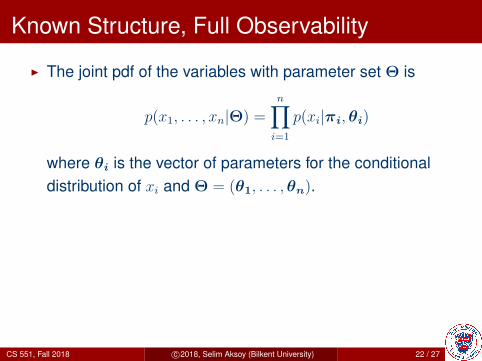
I The joint pdf of the variables with parameter set Θ is
p(x1, . . . , xn|Θ) =n∏
i=1
p(xi|πi,θi)
where θi is the vector of parameters for the conditionaldistribution of xi and Θ = (θ1, . . . ,θn).
I Given training data X = {x1, . . . ,xm} wherexl = (xl1, . . . , xln)
T , the log-likelihood of Θ with respect to Xcan be computed as
logL(Θ|X ) =m∑l=1
n∑i=1
log p(xli|πi,θi).
CS 551, Fall 2018 c©2018, Selim Aksoy (Bilkent University) 22 / 27

Known Structure, Full Observability
I The likelihood decomposes according to the structure of thenetwork so we can compute the MLEs for each nodeindependently.
I An alternative is to assign a prior probability densityfunction p(θi) to each θi and use the training data X tocompute the posterior distribution p(θi|X ) and the Bayesestimate Ep(θi|X )[θi].
I We will study the special case of discrete variables withdiscrete parents.
CS 551, Fall 2018 c©2018, Selim Aksoy (Bilkent University) 23 / 27
Known Structure, Full Observability
I Let each discrete variable xi have ri possible values(states) with probabilities
p(xi = k|πi = j,θi) = θijk > 0
where k ∈ {1, . . . , ri}, j is the state of xi’s parents andθi = {θijk} specifies the parameters of the multinomialdistribution for every combination of πi.
I Given X , the MLE of θijk can be computed as
θ̂ijk =Nijk
Nij
where Nijk is the number of cases in X in which xi = k andπi = j, and Nij =
∑rik=1Nijk.
CS 551, Fall 2018 c©2018, Selim Aksoy (Bilkent University) 24 / 27
Known Structure, Full Observability
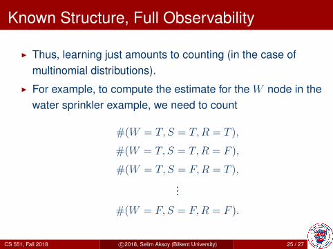
I Thus, learning just amounts to counting (in the case ofmultinomial distributions).
I For example, to compute the estimate for the W node in thewater sprinkler example, we need to count
#(W = T, S = T,R = T ),
#(W = T, S = T,R = F ),
#(W = T, S = F,R = T ),
...
#(W = F, S = F,R = F ).
CS 551, Fall 2018 c©2018, Selim Aksoy (Bilkent University) 25 / 27
Known Structure, Full Observability
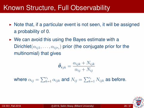
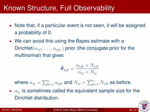
I Note that, if a particular event is not seen, it will be assigneda probability of 0.
I We can avoid this using the Bayes estimate with aDirichlet(αij1, . . . , αijri) prior (the conjugate prior for themultinomial) that gives
θ̂ijk =αijk +Nijk
αij +Nij
where αij =∑ri
k=1 αijk and Nij =∑ri
k=1Nijk as before.
I αij is sometimes called the equivalent sample size for theDirichlet distribution.
CS 551, Fall 2018 c©2018, Selim Aksoy (Bilkent University) 26 / 27
Known Structure, Full Observability
I Note that, if a particular event is not seen, it will be assigneda probability of 0.
I We can avoid this using the Bayes estimate with aDirichlet(αij1, . . . , αijri) prior (the conjugate prior for themultinomial) that gives
θ̂ijk =αijk +Nijk
αij +Nij
where αij =∑ri
k=1 αijk and Nij =∑ri
k=1Nijk as before.
I αij is sometimes called the equivalent sample size for theDirichlet distribution.
CS 551, Fall 2018 c©2018, Selim Aksoy (Bilkent University) 26 / 27
Naive Bayesian Network
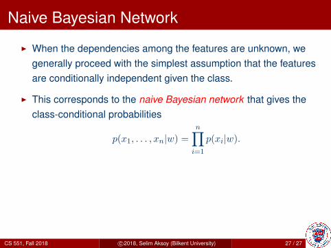
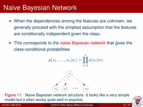
I When the dependencies among the features are unknown, wegenerally proceed with the simplest assumption that the featuresare conditionally independent given the class.
I This corresponds to the naive Bayesian network that gives theclass-conditional probabilities
p(x1, . . . , xn|w) =n∏
i=1
p(xi|w).
. . .x2x1 xn
w
Figure 11: Naive Bayesian network structure. It looks like a very simplemodel but it often works quite well in practice.
CS 551, Fall 2018 c©2018, Selim Aksoy (Bilkent University) 27 / 27
Naive Bayesian Network
I When the dependencies among the features are unknown, wegenerally proceed with the simplest assumption that the featuresare conditionally independent given the class.
I This corresponds to the naive Bayesian network that gives theclass-conditional probabilities
p(x1, . . . , xn|w) =n∏
i=1
p(xi|w).
. . .x2x1 xn
w
Figure 11: Naive Bayesian network structure. It looks like a very simplemodel but it often works quite well in practice.
CS 551, Fall 2018 c©2018, Selim Aksoy (Bilkent University) 27 / 27