probabilistic rewrite theories: unifying models, logics ... · probabilistic rewrite theories:...

Probabilistic Rewrite Theories:Unifying Models, Logics and Tools

Nirman Kumar, Koushik Sen, Jose Meseguer, Gul AghaDepartment of Computer Science,

University of Illinois at Urbana-Champaign.nkumar5,ksen,meseguer,[email protected]

Abstract. Probabilistic rewrite theories are proposed as a general se-mantic framework that unifies many existing models of probabilistic sys-tems for both discrete and continuous time and suggests new models suchas probabilistic hybrid systems. Probabilistic temporal logics for existingmodels are likewise unified in two logics, namely PRTL and PRTL∗ thatwe develop. Having a common semantic framework enables rigorouslyspecified combinations of existing modelling and model checking toolsthat are based on different models–including the PMaude interpreterthat can execute finitary probabilistic rewrite theory specifications.

Keywords: rewriting logic, probabilistic systems, stochastic systems,pmaude

1 Introduction

Large scale concurrent systems can be very complex. In modelling such systems,it is infeasible to account for the complex interplay of the various different factorsthat affect events in the system. For example, in a large scale computer networklike the Internet, network delays, congestion and failures affect each other in waysthat make it impossible to model the system deterministically. Furthermore,nondeterministic models do not allow us to model the likely behavior of thesystem. Probabilistic analysis has often been used to understand such complexsystems better.

A probabilistic model allows us to quantify a number of sources of inde-terminacy in concurrent systems. The exact time duration of a behavior oftendepends on the schedulers, loads, etc. and may be represented by a stochasticprocess. Process or network failures may occur with a certain rate. Randomnesscan also come in explicitly: some parts of the system may implement random-ized algorithms. An appropriate framework for probabilistic modelling is needed,which permits questions such as: “What is the mean throughput?”, “What isthe probability of a successful delivery in the next 10 seconds?” and so on.

There has been considerable research on models, logics and verification ofprobabilistic systems. Work in this area includes probabilistic nondeterminis-tic systems [5, 12], probabilistic Petri nets [28, 30] and probabilistic algebra ap-proaches [23, 22]. Logics such as Continuous Stochastic logic (CSL) [1, 2], Proba-bilistic Computational Tree Logic (pCTL) and Probabilistic CTL∗ (pCTL∗) [5]are some of the logics typically used to express properties for the above models.

2

For some of these logics, tools have been developed to support model checkingspecifications (e.g., PRISM [27] and ETMCC [20]). Other tools – UltraSan [11],SPNP [9], PEPA workbench [16] and GreatSPN [7]– have been used for perfor-mance analysis of CTMCs [24]. These tools have also been applied to severalreal world applications. For example, [26, 15] consider verification of a wirelessnetwork protocol and QoS management using a monitoring and evaluation ap-proach.

It is useful to distinguish between a system specification – in which the systemwe want to study is specified using a particular formalism such as stochasticPetri net – and a property specification – in which specific properties such assafety or performance that the system satisfies are specified using a logic suchas probabilistic temporal logic. This distinction corresponds to the differencebetween semantic models and property logics.

Although a number of semantics models and property logics have been devel-oped, there has as yet been no semantic unification of these different formalisms.We propose probabilistic rewrite theories as a way of achieving such a semanticunification. Rewriting logic [31] has already been shown to be a natural anduseful semantic framework which unifies different kinds of concurrent systems[31, 33], as well as models of real time and hybrid systems [37].

In a standard rewrite theory, transitions in a system are described by labelledrewrite rules of the form,

l : t −→ t′ if cond

Intuitively, a rule of this form specifies a pattern t such that, if some fragmentof the system’s state matches that pattern and satisfies the condition cond, thena local transition of that state fragment changing into the pattern t′ can takeplace. In a probabilistic rewrite rule we add probability information to such rules.Specifically, our proposed probabilistic rules are of the form,

l : t(−→x ) −→ t′(−→x ,−→y ) if cond(−→x ) with probability π(−→x ).

The rule will match a state fragment if there is a substitution θ for the variables−→x that makes θ(t) equal to that state fragment and satisfies θ(cond). Because t′

is of the form t′(−→x ,−→y ), the next state is not uniquely determined: it depends onthe choice of an additional substitution ρ for the variables −→y . Thus the result ofapplying the rule may be nondeterministic. The choice of ρ is made according tothe probability function θ(π), which in general is not a fixed probability function,but a family of functions: one for each match θ of the variables −→x .

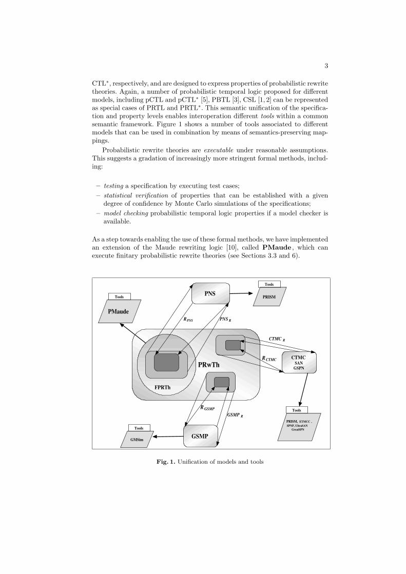
It turns out that this general notion of probabilistic rewrite rule can be usedto naturally represent the different models of probabilistic systems mentionedabove. Figure 1 shows semantics-preserving mappings from such models into thecommon framework of probabilistic rewrite theories. Inverse mappings definedon appropriate subclasses are also shown. This provides a semantic unificationat the system specification level. Furthermore, probabilistic rewrite theories canmodel hybrid probabilistic systems. At present, the commonly used models haveat most only one continuously varying quantity, namely time. However proba-bilistic rewrite theories can also specify hybrid systems in which different pa-rameters besides time change continuously. For property level specifications wepropose probabilistic rewriting temporal logic (PRTL and PRTL∗) as a unify-ing temporal logic. PRTL and PRTL∗ are probabilistic extensions of CTL and

3

CTL∗, respectively, and are designed to express properties of probabilistic rewritetheories. Again, a number of probabilistic temporal logic proposed for differentmodels, including pCTL and pCTL∗ [5], PBTL [3], CSL [1, 2] can be representedas special cases of PRTL and PRTL∗. This semantic unification of the specifica-tion and property levels enables interoperation different tools within a commonsemantic framework. Figure 1 shows a number of tools associated to differentmodels that can be used in combination by means of semantics-preserving map-pings.

Probabilistic rewrite theories are executable under reasonable assumptions.This suggests a gradation of increasingly more stringent formal methods, includ-ing:

– testing a specification by executing test cases;– statistical verification of properties that can be established with a given

degree of confidence by Monte Carlo simulations of the specifications;– model checking probabilistic temporal logic properties if a model checker is

available.

As a step towards enabling the use of these formal methods, we have implementedan extension of the Maude rewriting logic [10], called PMaude , which canexecute finitary probabilistic rewrite theories (see Sections 3.3 and 6).

PNS

FPRTh

R PNS PNS R

PRwTh

CTMC SAN

GSPN

GSMP

R GSMP

GSMP R

R CTMC

CTMC R

PRISM

Tools

PMaude

Tools

GMSim

Tools

PRISM, ETMCC ,

SPNP, UltraSAN

GreatSPN

Tools

Fig. 1. Unification of models and tools

4

This paper is organized as follows. Section 2 provides several definitions thatare required for defining probabilistic rewrite theories. Section 3 defines the con-cept and semantics of a probabilistic rewrite theory in all generality. Section 4shows how various well known models for probabilistic systems can be repre-sented as probabilistic rewrite theories. Section 5 defines probabilistic temporallogics for expressing properties of probabilistic rewrite theories. Section 6 pro-vides details of PMaude, an implementation of finitary probabilistic rewritetheories (see Section 3.3) in Maude. We conclude by discussing directions forfuture research work. An appendix provides Maude code and sample executionsfor two examples specified in PMaude.

2 Background

We provide here the definitions of σ-algebra, probability spaces, F-covers, mem-bership equational theories, canonical ground substitutions, equivalence of sub-stitutions and rewrite theories needed in the rest of the paper.

Definition 1 (σ-algebra). A σ-algebra on a set X is a nonempty collection ofsubsets F of X such that

(i) X ∈ F ,(ii) A ∈ F =⇒ X −A ∈ F ,(iii) I ⊆ N, Ai ∈ F for each i ∈ I =⇒ ⋃

i∈I Ai ∈ F .

We denote by BR the smallest σ-algebra on R containing the sets (−∞, x] for allx ∈ R.

Definition 2 (Probability space). A probability space is a triple (X,F , π)with F a σ-algebra on X, and π : F → [0, 1] a function such that:

(i) π(X) = 1 and π(∅) = 0,(ii) Given a subset I ⊆ N, a family Ai, i ∈ I, with Ai ∈ F for each i and

Ai ∩Aj = ∅ for i 6= j, then π(⋃

i∈I Ai) =∑

i∈I π(Ai).

Here π is known as the probability measure function. For a given σ-algebra Fon X, we denote by

PFun(X,F) = π | (X,F , π) is a probability spaceDefinition 3 (F-cover). An F-cover for a σ-algebra F on X, is a functionα : X → F , such that ∀x ∈ X . x ∈ α(x).

For a given probability space (X,F , π), an F-cover α naturally defines a functionα;π from X to [0, 1]. Thus, for example, with X = R and F = BR, we can defineα to be the function that maps the real number x to the set (−∞, x]. With X afinite set and F = P(X), the power set of X, it is natural to define α to be thefunction that maps x ∈ X to the singleton x.

A membership equational theory [32] is a pair (Σ, E), with Σ a signatureconsisting of a set K of kinds, for each k ∈ K a set Sk of sorts, and a set ofoperator declarations of the form f : k1 . . . kn −→ k, with k, k1, . . . , kn ∈ K, andwith E a set of conditional Σ-equations and Σ-memberships of the form,

5

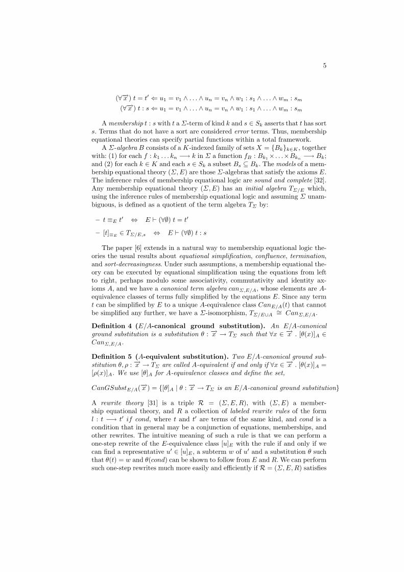
(∀−→x ) t = t′ ⇐ u1 = v1 ∧ . . . ∧ un = vn ∧ w1 : s1 ∧ . . . ∧ wm : sm

(∀−→x ) t : s ⇐ u1 = v1 ∧ . . . ∧ un = vn ∧ w1 : s1 ∧ . . . ∧ wm : sm

A membership t : s with t a Σ-term of kind k and s ∈ Sk asserts that t has sorts. Terms that do not have a sort are considered error terms. Thus, membershipequational theories can specify partial functions within a total framework.

A Σ-algebra B consists of a K-indexed family of sets X = Bkk∈K , togetherwith: (1) for each f : k1 . . . kn −→ k in Σ a function fB : Bk1× . . .×Bkn

−→ Bk;and (2) for each k ∈ K and each s ∈ Sk a subset Bs ⊆ Bk. The models of a mem-bership equational theory (Σ,E) are those Σ-algebras that satisfy the axioms E.The inference rules of membership equational logic are sound and complete [32].Any membership equational theory (Σ, E) has an initial algebra TΣ/E which,using the inference rules of membership equational logic and assuming Σ unam-biguous, is defined as a quotient of the term algebra TΣ by:

– t ≡E t′ ⇔ E ` (∀∅) t = t′

– [t]≡E ∈ TΣ/E,s ⇔ E ` (∀∅) t : s

The paper [6] extends in a natural way to membership equational logic the-ories the usual results about equational simplification, confluence, termination,and sort-decreasingness. Under such assumptions, a membership equational the-ory can be executed by equational simplification using the equations from leftto right, perhaps modulo some associativity, commutativity and identity ax-ioms A, and we have a canonical term algebra canΣ,E/A, whose elements are A-equivalence classes of terms fully simplified by the equations E. Since any termt can be simplified by E to a unique A-equivalence class CanE/A(t) that cannotbe simplified any further, we have a Σ-isomorphism, TΣ/E∪A

∼= CanΣ,E/A.

Definition 4 (E/A-canonical ground substitution). An E/A-canonicalground substitution is a substitution θ : −→x → TΣ such that ∀x ∈ −→x . [θ(x)]A ∈CanΣ,E/A.

Definition 5 (A-equivalent substitution). Two E/A-canonical ground sub-stitution θ, ρ : −→x → TΣ are called A-equivalent if and only if ∀x ∈ −→x . [θ(x)]A =[ρ(x)]A. We use [θ]A for A-equivalence classes and define the set,

CanGSubstE/A(−→x ) = [θ]A | θ : −→x → TΣ is an E/A-canonical ground substitution

A rewrite theory [31] is a triple R = (Σ,E, R), with (Σ, E) a member-ship equational theory, and R a collection of labeled rewrite rules of the forml : t −→ t′ if cond, where t and t′ are terms of the same kind, and cond is acondition that in general may be a conjunction of equations, memberships, andother rewrites. The intuitive meaning of such a rule is that we can perform aone-step rewrite of the E-equivalence class [u]E with the rule if and only if wecan find a representative u′ ∈ [u]E , a subterm w of u′ and a substitution θ suchthat θ(t) = w and θ(cond) can be shown to follow from E and R. We can performsuch one-step rewrites much more easily and efficiently if R = (Σ,E, R) satisfies

6

the following executability requirements: (i) the equations E are confluent, ter-minating, and sort-decreasing modulo axioms A; and (ii) the rules R are coherent[38] relative to E modulo A. Coherence states that if a representative u′ ∈ [u]Ecan be directly rewritten by a rule in R to a term v, then it is also possible todirectly perform a one-step rewrite with R of a representative w ∈ CanE/A(u′)to a term v′ in such a way that canE/A(v) = canE/A(v′). We call the rewritecanE/A(u′) −→ canE/A(v′) a canonical one-step rewrite modulo A. Coherenceensures that all one-step rewrites at the level of E-equivalence classes can besimulated by the much simpler canonical one-step rewrites modulo A.

3 Probabilistic Rewrite Theories

We define here probabilistic rewrite theories and the notions of computation andadversary. We then define a probability space on the set of computation pathsand give a probability measure function on this space. We conclude by definingan important class of rewrite theories, called finitary rewrite theories, which canbe viewed as a restricted class of probabilistic rewrite theories.

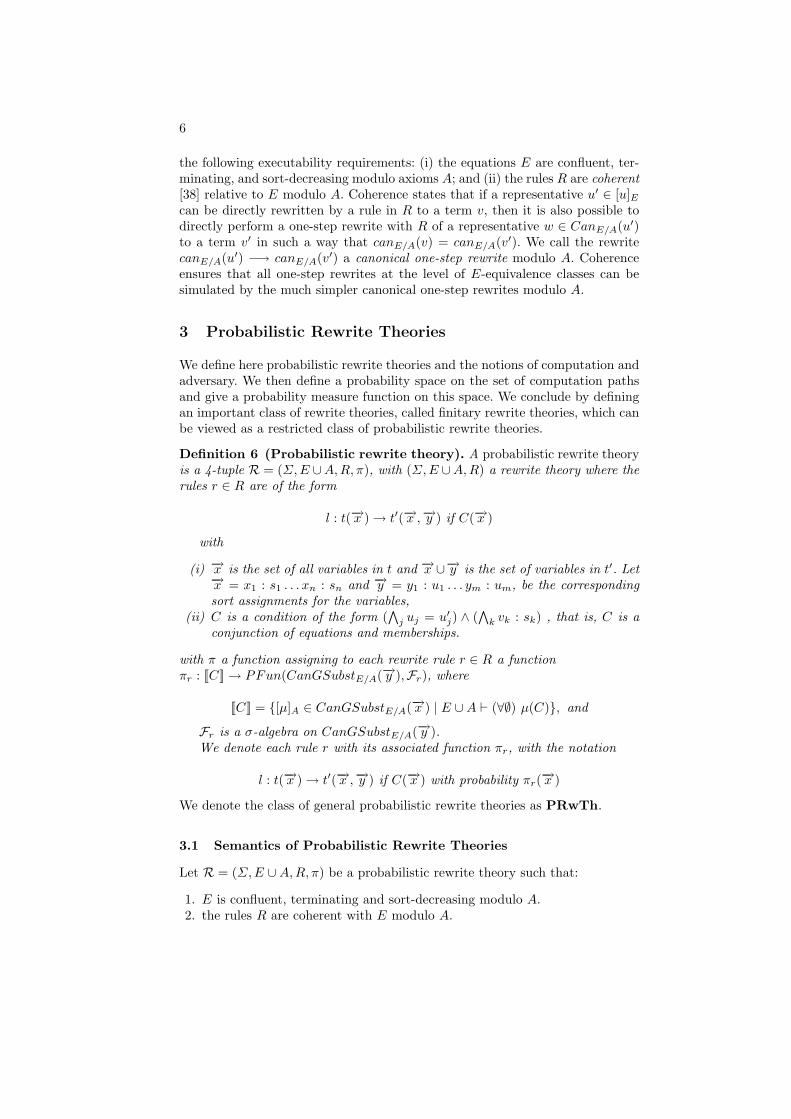
Definition 6 (Probabilistic rewrite theory). A probabilistic rewrite theoryis a 4-tuple R = (Σ,E ∪A,R, π), with (Σ, E ∪A,R) a rewrite theory where therules r ∈ R are of the form

l : t(−→x ) → t′(−→x ,−→y ) if C(−→x )

with

(i) −→x is the set of all variables in t and −→x ∪−→y is the set of variables in t′. Let−→x = x1 : s1 . . . xn : sn and −→y = y1 : u1 . . . ym : um, be the correspondingsort assignments for the variables,

(ii) C is a condition of the form (∧

j uj = u′j) ∧ (∧

k vk : sk) , that is, C is aconjunction of equations and memberships.

with π a function assigning to each rewrite rule r ∈ R a functionπr : [[C]] → PFun(CanGSubstE/A(−→y ),Fr), where

[[C]] = [µ]A ∈ CanGSubstE/A(−→x ) | E ∪A ` (∀∅) µ(C), and

Fr is a σ-algebra on CanGSubstE/A(−→y ).We denote each rule r with its associated function πr, with the notation

l : t(−→x ) → t′(−→x ,−→y ) if C(−→x ) with probability πr(−→x )

We denote the class of general probabilistic rewrite theories as PRwTh.

3.1 Semantics of Probabilistic Rewrite Theories

Let R = (Σ,E ∪A,R, π) be a probabilistic rewrite theory such that:

1. E is confluent, terminating and sort-decreasing modulo A.2. the rules R are coherent with E modulo A.

7

We also assume a choice for each rule r of an Fr-cover αr :CanGSubstE/A(−→y ) → Fr. This Fr-cover will be used to assign probabilitiesto rewrite steps. Its choice will depend on the particular problem under consid-eration.

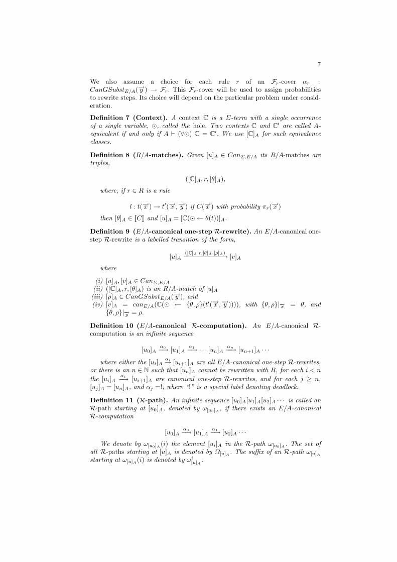
Definition 7 (Context). A context C is a Σ-term with a single occurrenceof a single variable, ¯, called the hole. Two contexts C and C′ are called A-equivalent if and only if A ` (∀¯) C = C′. We use [C]A for such equivalenceclasses.

Definition 8 (R/A-matches). Given [u]A ∈ CanΣ,E/A its R/A-matches aretriples,

([C]A, r, [θ]A),

where, if r ∈ R is a rule

l : t(−→x ) → t′(−→x ,−→y ) if C(−→x ) with probability πr(−→x )

then [θ]A ∈ [[C]] and [u]A = [C(¯ ← θ(t))]A.

Definition 9 (E/A-canonical one-step R-rewrite). An E/A-canonical one-step R-rewrite is a labelled transition of the form,

[u]A([C]A,r,[θ]A,[ρ]A)−−−−−−−−−−−→ [v]A

where

(i) [u]A, [v]A ∈ CanΣ,E/A

(ii) ([C]A, r, [θ]A) is an R/A-match of [u]A(iii) [ρ]A ∈ CanGSubstE/A(−→y ), and(iv) [v]A = canE/A(C(¯ ← θ, ρ(t′(−→x ,−→y )))), with θ, ρ|−→x = θ, and

θ, ρ|−→y = ρ.

Definition 10 (E/A-canonical R-computation). An E/A-canonical R-computation is an infinite sequence

[u0]Aα0−→ [u1]A

α1−→ · · · [un]Aαn−−→ [un+1]A · · ·

where either the [ui]Aαi→ [ui+1]A are all E/A-canonical one-step R-rewrites,

or there is an n ∈ N such that [un]A cannot be rewritten with R, for each i < n

the [ui]Aαi−→ [ui+1]A are canonical one-step R-rewrites, and for each j ≥ n,

[uj ]A = [un]A, and αj =!, where “!” is a special label denoting deadlock.

Definition 11 (R-path). An infinite sequence [u0]A[u1]A[u2]A · · · is called anR-path starting at [u0]A, denoted by ω[u0]A , if there exists an E/A-canonicalR-computation

[u0]Aα0−→ [u1]A

α1−→ [u2]A · · ·We denote by ω[u0]A(i) the element [ui]A in the R-path ω[u0]A . The set of

all R-paths starting at [u]A is denoted by Ω[u]A . The suffix of an R-path ω[u]A

starting at ω[u]A(i) is denoted by ωi[u]A

.

8

Definition 12 (Borel σ-algebra on Ω[u]A). Let [u]A[u1]A · · · [un]A ∈(CanΣ,E/A,k)+ be a finite word, that we denote as w[u]A to emphasize its first el-ement. Then we define the basic cylinder set for w[u]A as the set ω[u]A ∈ Ω[u]A |∀ 1 ≤ i ≤ n . ω[u]A(i) = w[u]A(i). Let B[u]A ⊆ P(Ω[u]A) be the smallest σ-algebraon Ω[u]A that contains the basic cylinder sets for all w[u]A ∈ (CanΣ,E/A,k)+. Thisalgebra is called the Borel σ-algebra of the basic cylinder sets.

The presence of nondeterminism in the choice of R/A-matches prevents us fromdefining a probability measure function on B[u]A . However we can resolve thisnondeterminism by the use of an adversary as defined below.

Definition 13 (Adversary). An adversary aR is a function that mapseach sequence [u0]A[u1]A · · · [un]A ∈ (CanΣ,E/A,k)∗ such that the sequence[u0]A[u1]A · · · [un]A is the finite prefix of some R-path starting at [u0]A, to aprobability distribution on the R/A-matches of [un]A.

Let AdvR be the set of all such adversaries. We can associate to a given proba-bilistic rewrite theory R a subset A ⊆ AdvR as its set of legal adversaries.

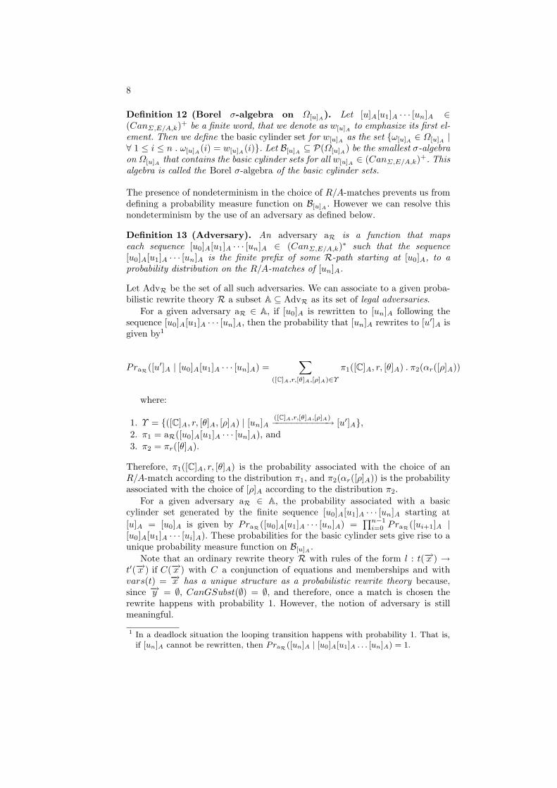
For a given adversary aR ∈ A, if [u0]A is rewritten to [un]A following thesequence [u0]A[u1]A · · · [un]A, then the probability that [un]A rewrites to [u′]A isgiven by1

PraR([u′]A | [u0]A[u1]A · · · [un]A) =∑

([C]A,r,[θ]A,[ρ]A)∈Υ

π1([C]A, r, [θ]A) . π2(αr([ρ]A))

where:

1. Υ = ([C]A, r, [θ]A, [ρ]A) | [un]A([C]A,r,[θ]A,[ρ]A)−−−−−−−−−−−→ [u′]A,

2. π1 = aR([u0]A[u1]A · · · [un]A), and3. π2 = πr([θ]A).

Therefore, π1([C]A, r, [θ]A) is the probability associated with the choice of anR/A-match according to the distribution π1, and π2(αr([ρ]A)) is the probabilityassociated with the choice of [ρ]A according to the distribution π2.

For a given adversary aR ∈ A, the probability associated with a basiccylinder set generated by the finite sequence [u0]A[u1]A · · · [un]A starting at[u]A = [u0]A is given by PraR([u0]A[u1]A · · · [un]A) =

∏n−1i=0 PraR([ui+1]A |

[u0]A[u1]A · · · [ui]A). These probabilities for the basic cylinder sets give rise to aunique probability measure function on B[u]A .

Note that an ordinary rewrite theory R with rules of the form l : t(−→x ) →t′(−→x ) if C(−→x ) with C a conjunction of equations and memberships and withvars(t) = −→x has a unique structure as a probabilistic rewrite theory because,since −→y = ∅, CanGSubst(∅) = ∅, and therefore, once a match is chosen therewrite happens with probability 1. However, the notion of adversary is stillmeaningful.

1 In a deadlock situation the looping transition happens with probability 1. That is,if [un]A cannot be rewritten, then PraR([un]A | [u0]A[u1]A . . . [un]A) = 1.

9

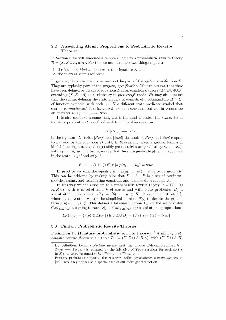
3.2 Associating Atomic Propositions to Probabilistic RewriteTheories

In Section 5 we will associate a temporal logic to a probabilistic rewrite theoryR = (Σ, E ∪A,R, π). For this we need to make two things explicit:

1. the intended kind k of states in the signature Σ and2. the relevant state predicates.

In general, the state predicates need not be part of the system specification R.They are typically part of the property specification. We can assume that theyhave been defined by means of equations D in an equational theory (Σ′, E∪A∪D)extending (Σ, E ∪ A) as a subtheory in protecting2 mode. We may also assumethat the syntax defining the state predicates consists of a subsignature Π ⊆ Σ′

of function symbols, with each p ∈ Π a different state predicate symbol thatcan be parameterized, that is, p need not be a constant, but can in general bean operator p : s1 . . . sn −→ Prop.

It is also useful to assume that, if k is the kind of states, the semantics ofthe state predicates Π is defined with the help of an operator,

|= : k [Prop] −→ [Bool]

in the signature Σ′ (with [Prop] and [Bool] the kinds of Prop and Bool respec-tively) and by the equations D ∪ A ∪ E. Specifically, given a ground term u ofkind k denoting a state and a (possibly parametric) state predicate p(u1, . . . , un),with u1, . . . , un ground terms, we say that the state predicate p(u1, . . . , un) holdsin the state [u]A if and only if,

E ∪A ∪D ` (∀ ∅) u |= p(u1, . . . , un) = true .

In practice we want the equality u |= p(u1, . . . , u1) = true to be decidable.This can be achieved by making sure that D ∪ A ∪ E is a set of confluent,sort-decreasing, and terminating equations and memberships modulo A.

In this way we can associate to a probabilistic rewrite theory R = (Σ, E ∪A,R, π) (with a selected kind k of states and with state predicates Π) aset of atomic predicates APΠ = θ(p) | p ∈ Π, θ ground substitution,where by convention we use the simplified notation θ(p) to denote the groundterm θ(p(x1, . . . , xn)). This defines a labeling function LΠ on the set of statesCanΣ,E/A,k assigning to each [u]A ∈ CanΣ,E/A,k the set of atomic propositions,

LΠ([u]A) = θ(p) ∈ APΠ | (E ∪A ∪D) ` (∀ ∅) u |= θ(p) = true.

3.3 Finitary Probabilistic Rewrite Theories

Definition 14 (Finitary probabilistic rewrite theory). 3 A finitary prob-abilistic rewrite theory is a 4-tuple Rf = (Σ,E ∪ A, R, γ), with (Σ, E ∪ A,R)2 By definition, being protecting means that the unique Σ-homomorphism h :

TΣ/E −→ TΣ′/E∪D|Σ ensured by the initiality of TΣ/E restricts for each sort sin Σ to a bijective function hs : TΣ/E,s −→ TΣ′/E∪D,s.

3 Finitary probabilistic rewrite theories were called probabilistic rewrite theories in[25]. Here they appear as a special case of our more general notion.

10

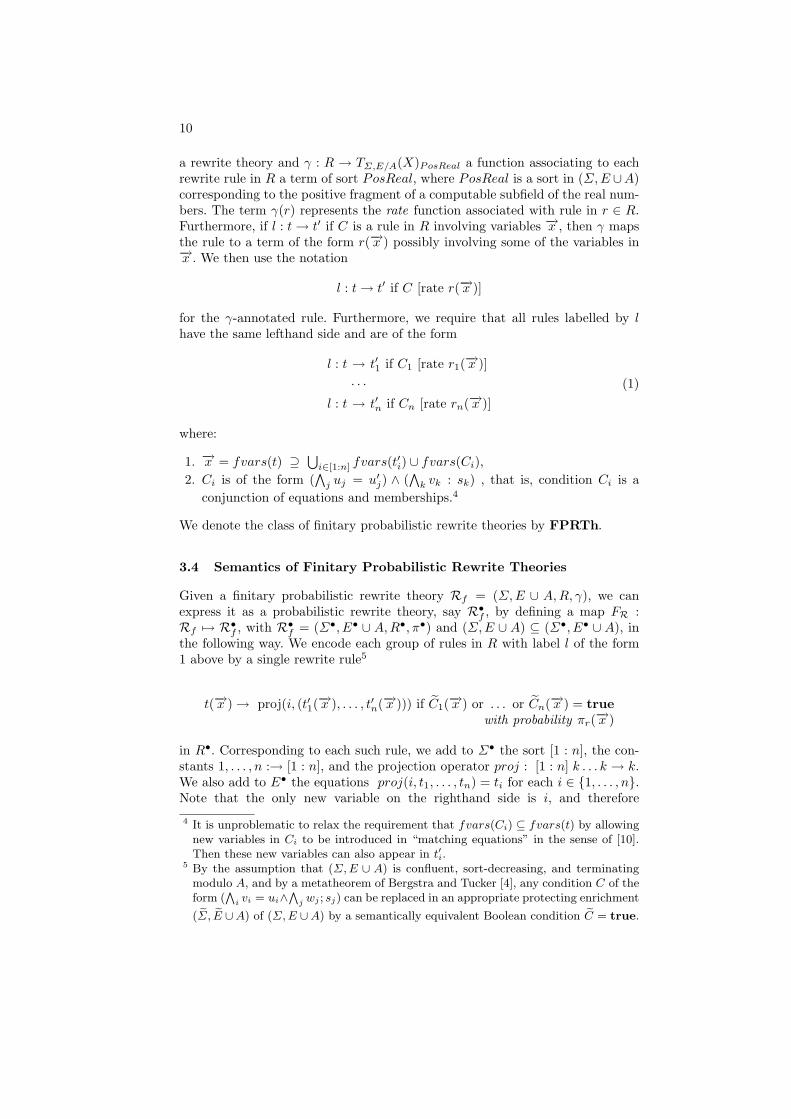
a rewrite theory and γ : R → TΣ,E/A(X)PosReal a function associating to eachrewrite rule in R a term of sort PosReal, where PosReal is a sort in (Σ, E ∪A)corresponding to the positive fragment of a computable subfield of the real num-bers. The term γ(r) represents the rate function associated with rule in r ∈ R.Furthermore, if l : t → t′ if C is a rule in R involving variables −→x , then γ mapsthe rule to a term of the form r(−→x ) possibly involving some of the variables in−→x . We then use the notation

l : t → t′ if C [rate r(−→x )]

for the γ-annotated rule. Furthermore, we require that all rules labelled by lhave the same lefthand side and are of the form

l : t → t′1 if C1 [rate r1(−→x )]· · · (1)

l : t → t′n if Cn [rate rn(−→x )]

where:

1. −→x = fvars(t) ⊇ ⋃i∈[1:n] fvars(t′i) ∪ fvars(Ci),

2. Ci is of the form (∧

j uj = u′j) ∧ (∧

k vk : sk) , that is, condition Ci is aconjunction of equations and memberships.4

We denote the class of finitary probabilistic rewrite theories by FPRTh.

3.4 Semantics of Finitary Probabilistic Rewrite Theories

Given a finitary probabilistic rewrite theory Rf = (Σ, E ∪ A, R, γ), we canexpress it as a probabilistic rewrite theory, say R•f , by defining a map FR :Rf 7→ R•f , with R•f = (Σ•, E• ∪ A,R•, π•) and (Σ, E ∪ A) ⊆ (Σ•, E• ∪ A), inthe following way. We encode each group of rules in R with label l of the form1 above by a single rewrite rule5

t(−→x ) → proj(i, (t′1(−→x ), . . . , t′n(−→x ))) if C1(−→x ) or . . . or Cn(−→x ) = true

with probability πr(−→x )

in R•. Corresponding to each such rule, we add to Σ• the sort [1 : n], the con-stants 1, . . . , n :→ [1 : n], and the projection operator proj : [1 : n] k . . . k → k.We also add to E• the equations proj(i, t1, . . . , tn) = ti for each i ∈ 1, . . . , n.Note that the only new variable on the righthand side is i, and therefore

4 It is unproblematic to relax the requirement that fvars(Ci) ⊆ fvars(t) by allowingnew variables in Ci to be introduced in “matching equations” in the sense of [10].Then these new variables can also appear in t′i.

5 By the assumption that (Σ, E ∪ A) is confluent, sort-decreasing, and terminatingmodulo A, and by a metatheorem of Bergstra and Tucker [4], any condition C of theform (

∧i vi = ui∧

∧j wj ; sj) can be replaced in an appropriate protecting enrichment

(Σ, E ∪A) of (Σ, E ∪A) by a semantically equivalent Boolean condition C = true.

11

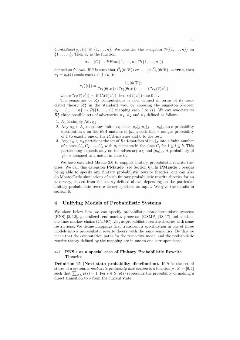
CanGSubstE/A(i) ∼= 1, . . . , n. We consider the σ-algebra P(1, . . . , n) on1, . . . , n. Then πr is the function

πr : [[C]] → PFun(1, . . . , n,P(1, . . . , n))defined as follows. If θ is such that C1(θ(−→x )) or . . . or Cn(θ(−→x )) = true, thenπ1 = πr(θ) sends each i ∈ [1 : n] to,

π1(i) =?ri(θ(−→x ))

?r1(θ(−→x ))+?r2(θ(−→x )) + · · ·+?rn(θ(−→x ))

where ?ri(θ(−→x )) = if Ci(θ(−→x )) then ri(θ(−→x )) else 0 fi .The semantics of Rf computations is now defined in terms of its asso-

ciated theory R•f in the standard way, by choosing the singleton F-coverαr : 1, . . . , n → P(1, . . . , n) mapping each i to i. We can associate toR•f three possible sets of adversaries A1, A2 and A3 defined as follows:

1. A1 is simply AdvR•f .2. Any aR ∈ A2 maps any finite sequence [u0]A[u1]A · · · [un]A to a probability

distribution π on the R/A-matches of [un]A such that π assigns probabilityof 1 to exactly one of the R/A-matches and 0 to the rest.

3. Any aR ∈ A3 partitions the set of R/A-matches of [un]A into a finite numberof classes C1, C2, . . . , Ck with ni elements in the class Ci for 1 ≤ i ≤ k. Thispartitioning depends only on the adversary aR and [un]A. A probability of

1kni

is assigned to a match in class Ci.

We have extended Maude 2.0 to support finitary probabilistic rewrite the-ories. We call this extension PMaude (see Section 6). In PMaude , besidesbeing able to specify any finitary probabilistic rewrite theories, one can alsodo Monte-Carlo simulations of such finitary probabilistic rewrite theories for anadversary, chosen from the set A3 defined above, depending on the particularfinitary probabilistic rewrite theory specified as input. We give the details insection 6.

4 Unifying Models of Probabilistic Systems

We show below how we can specify probabilistic non-deterministic systems(PNS) [5, 12], generalized semi-markov processes (GSMP) [18, 17] and continu-ous time markov chains (CTMC) [24], as probabilistic rewrite theories with somerestrictions. We define mappings that transform a specification in one of thosemodels into a probabilistic rewrite theory with the same semantics. By this wemean that the computation paths for the respective model and the probabilisticrewrite theory defined by the mapping are in one-to-one correspondence.

4.1 PNS’s as a special case of Finitary Probabilistic RewriteTheories

Definition 15 (Next-state probability distribution). If S is the set ofstates of a system, a next-state probability distribution is a function p : S → [0, 1]such that

∑s∈S p(s) = 1. For s ∈ S, p(s) represents the probability of making a

direct transition to s from the current state.

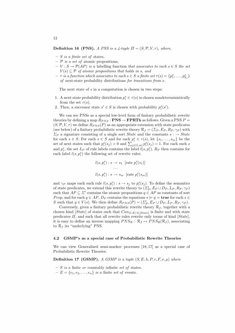
12

Definition 16 (PNS). A PNS is a 4-tuple Π = (S,P, V, τ), where,

– S is a finite set of states,– P is a set of atomic propositions,– V : S → P(AP ) is a labelling function that associates to each s ∈ S the set

V (s) ⊆ P of atomic propositions that holds in s, and– τ is a function which associates to each s ∈ S a finite set τ(s) = ps

1, . . . , psks

of next-state probability distributions for transitions from s.

The next state of s in a computation is chosen in two steps:

1. A next-state probability distribution psi ∈ τ(s) is chosen nondeterministically

from the set τ(s),2. Then, a successor state s′ ∈ S is chosen with probability ps

i (s′).

We can see PNSs as a special low-level form of finitary probabilistic rewritetheories by defining a map RPNS : PNS→ FPRTh as follows. Given a PNS P =(S,P, V, τ) we define RPNS(P ) as an appropriate extension with state predicates(see below) of a finitary probabilistic rewrite theoryRf = (ΣP , EP , RP , γP ) withΣP a signature consisting of a single sort State and the constants s : → Statefor each s ∈ S. For each s ∈ S and for each ps

i ∈ τ(s), let s1, . . . , sm be theset of next states such that ps

i (sj) > 0 and∑

j∈[1,m] psi (sj) = 1. For each such s

and psi , the set LP of rule labels contains the label l(s, ps

i ). RP then contains foreach label l(s, ps

i ) the following set of rewrite rules:

l(s, psi ) : s → s1 [rate ps

i (s1)]· · ·

l(s, psi ) : s → sm [rate ps

i (sm)]

and γP maps each such rule l(s, psi ) : s → sj to ps

i (sj). To define the semanticsof state predicates, we extend this rewrite theory to (Σ′

P , EP ∪DP , LP , RP , γP )such that AP ⊆ Σ′ contains the atomic propositions q ∈ AP as constants of sortProp, and for each q ∈ AP , DP contains the equations s |= q = true for each s ∈S such that q ∈ V (s). We then define RPNS(P ) = (Σ′

P , EP ∪DP , LP , RP , γP ).Conversely, given a finitary probabilistic rewrite theory Rf , together with a

chosen kind [State] of states such that CanΣ,E/A,[State] is finite and with statepredicates Π, and such that all rewrite rules rewrite only terms of kind [State],it is easy to define an inverse mapping PNSR : Rf 7→ PNSR(Rf ), associatingto Rf its “underlying” PNS.

4.2 GSMP’s as a special case of Probabilistic Rewrite Theories

We can view Generalized semi-markov processes [18, 17] as a special case ofProbabilistic Rewrite Theories.

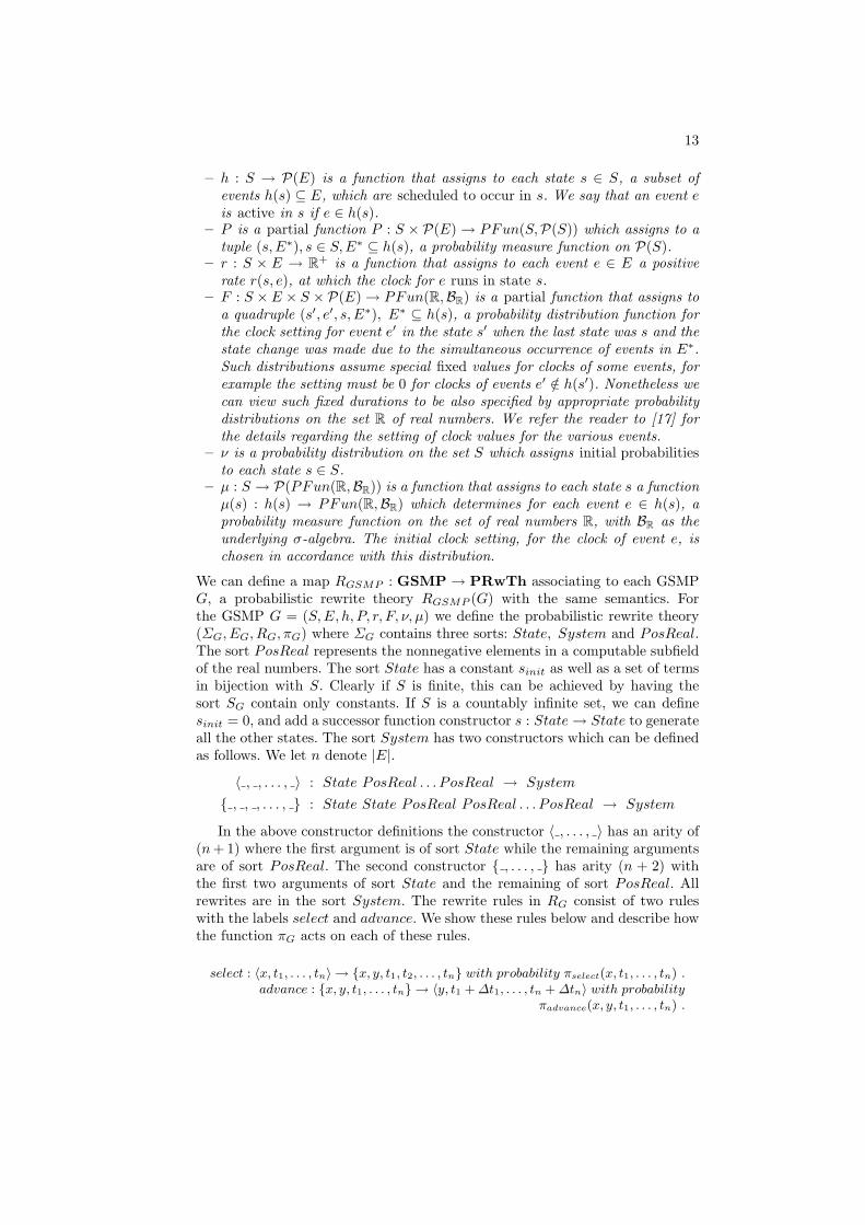
Definition 17 (GSMP). A GSMP is a tuple (S,E, h, P, r, F, ν, µ) where

– S is a finite or countably infinite set of states.– E = e1, e2, . . . , en is a finite set of events.

13

– h : S → P(E) is a function that assigns to each state s ∈ S, a subset ofevents h(s) ⊆ E, which are scheduled to occur in s. We say that an event eis active in s if e ∈ h(s).

– P is a partial function P : S × P(E) → PFun(S,P(S)) which assigns to atuple (s,E∗), s ∈ S, E∗ ⊆ h(s), a probability measure function on P(S).

– r : S × E → R+ is a function that assigns to each event e ∈ E a positiverate r(s, e), at which the clock for e runs in state s.

– F : S ×E × S ×P(E) → PFun(R,BR) is a partial function that assigns toa quadruple (s′, e′, s, E∗), E∗ ⊆ h(s), a probability distribution function forthe clock setting for event e′ in the state s′ when the last state was s and thestate change was made due to the simultaneous occurrence of events in E∗.Such distributions assume special fixed values for clocks of some events, forexample the setting must be 0 for clocks of events e′ /∈ h(s′). Nonetheless wecan view such fixed durations to be also specified by appropriate probabilitydistributions on the set R of real numbers. We refer the reader to [17] forthe details regarding the setting of clock values for the various events.

– ν is a probability distribution on the set S which assigns initial probabilitiesto each state s ∈ S.

– µ : S → P(PFun(R,BR)) is a function that assigns to each state s a functionµ(s) : h(s) → PFun(R,BR) which determines for each event e ∈ h(s), aprobability measure function on the set of real numbers R, with BR as theunderlying σ-algebra. The initial clock setting, for the clock of event e, ischosen in accordance with this distribution.

We can define a map RGSMP : GSMP → PRwTh associating to each GSMPG, a probabilistic rewrite theory RGSMP (G) with the same semantics. Forthe GSMP G = (S, E, h, P, r, F, ν, µ) we define the probabilistic rewrite theory(ΣG, EG, RG, πG) where ΣG contains three sorts: State, System and PosReal.The sort PosReal represents the nonnegative elements in a computable subfieldof the real numbers. The sort State has a constant sinit as well as a set of termsin bijection with S. Clearly if S is finite, this can be achieved by having thesort SG contain only constants. If S is a countably infinite set, we can definesinit = 0, and add a successor function constructor s : State → State to generateall the other states. The sort System has two constructors which can be definedas follows. We let n denote |E|.

〈 , , . . . , 〉 : State PosReal . . . PosReal → System

, , , . . . , : State State PosReal PosReal . . . PosReal → System

In the above constructor definitions the constructor 〈 , . . . , 〉 has an arity of(n + 1) where the first argument is of sort State while the remaining argumentsare of sort PosReal. The second constructor , . . . , has arity (n + 2) withthe first two arguments of sort State and the remaining of sort PosReal. Allrewrites are in the sort System. The rewrite rules in RG consist of two ruleswith the labels select and advance. We show these rules below and describe howthe function πG acts on each of these rules.

select : 〈x, t1, . . . , tn〉 → x, y, t1, t2, . . . , tn with probability πselect(x, t1, . . . , tn) .advance : x, y, t1, . . . , tn → 〈y, t1 + ∆t1, . . . , tn + ∆tn〉 with probability

πadvance(x, y, t1, . . . , tn) .

14

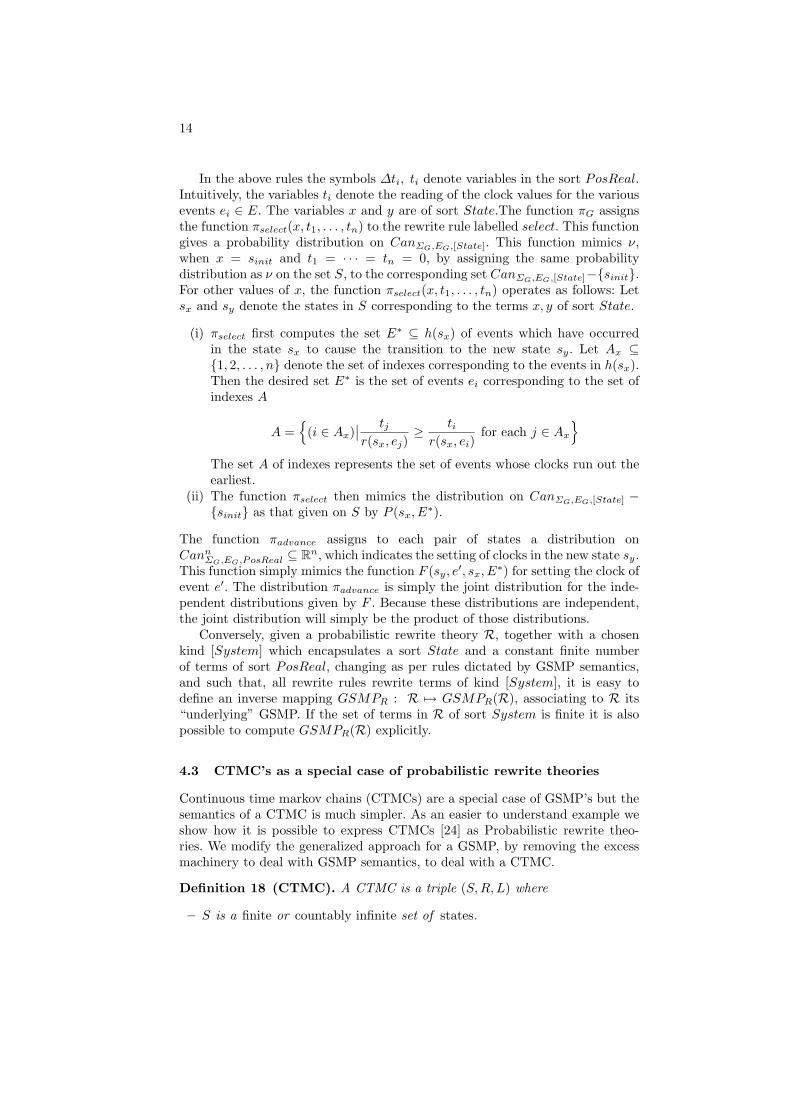
In the above rules the symbols ∆ti, ti denote variables in the sort PosReal.Intuitively, the variables ti denote the reading of the clock values for the variousevents ei ∈ E. The variables x and y are of sort State.The function πG assignsthe function πselect(x, t1, . . . , tn) to the rewrite rule labelled select. This functiongives a probability distribution on CanΣG,EG,[State]. This function mimics ν,when x = sinit and t1 = · · · = tn = 0, by assigning the same probabilitydistribution as ν on the set S, to the corresponding set CanΣG,EG,[State]−sinit.For other values of x, the function πselect(x, t1, . . . , tn) operates as follows: Letsx and sy denote the states in S corresponding to the terms x, y of sort State.

(i) πselect first computes the set E∗ ⊆ h(sx) of events which have occurredin the state sx to cause the transition to the new state sy. Let Ax ⊆1, 2, . . . , n denote the set of indexes corresponding to the events in h(sx).Then the desired set E∗ is the set of events ei corresponding to the set ofindexes A

A =

(i ∈ Ax)∣∣ tjr(sx, ej)

≥ tir(sx, ei)

for each j ∈ Ax

The set A of indexes represents the set of events whose clocks run out theearliest.

(ii) The function πselect then mimics the distribution on CanΣG,EG,[State] −sinit as that given on S by P (sx, E∗).

The function πadvance assigns to each pair of states a distribution onCann

ΣG,EG,PosReal ⊆ Rn, which indicates the setting of clocks in the new state sy.This function simply mimics the function F (sy, e′, sx, E∗) for setting the clock ofevent e′. The distribution πadvance is simply the joint distribution for the inde-pendent distributions given by F . Because these distributions are independent,the joint distribution will simply be the product of those distributions.

Conversely, given a probabilistic rewrite theory R, together with a chosenkind [System] which encapsulates a sort State and a constant finite numberof terms of sort PosReal, changing as per rules dictated by GSMP semantics,and such that, all rewrite rules rewrite terms of kind [System], it is easy todefine an inverse mapping GSMPR : R 7→ GSMPR(R), associating to R its“underlying” GSMP. If the set of terms in R of sort System is finite it is alsopossible to compute GSMPR(R) explicitly.

4.3 CTMC’s as a special case of probabilistic rewrite theories

Continuous time markov chains (CTMCs) are a special case of GSMP’s but thesemantics of a CTMC is much simpler. As an easier to understand example weshow how it is possible to express CTMCs [24] as Probabilistic rewrite theo-ries. We modify the generalized approach for a GSMP, by removing the excessmachinery to deal with GSMP semantics, to deal with a CTMC.

Definition 18 (CTMC). A CTMC is a triple (S,R, L) where

– S is a finite or countably infinite set of states.

15

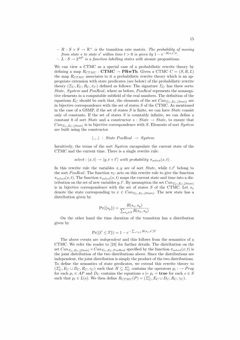
– R : S × S → R+ is the transition rate matrix. The probability of movingfrom state s to state s′ within time t > 0 is given by 1− e−R(s,s′)t.

– L : S → 2AP is a function labelling states with atomic propositions.

We can view a CTMC as a special case of a probabilistic rewrite theory bydefining a map RCTMC : CTMC → PRwTh. Given a CTMC C = (S, R,L)the map RCTMC associates to it a probabilistic rewrite theory which is an ap-propriate extension with state predicates (see below) of the probabilistic rewritetheory (ΣC , EC , RC , πC) defined as follows: The signature ΣC has three sorts:State, System and PosReal, where as before, PosReal represents the nonnega-tive elements in a computable subfield of the real numbers. The definition of theequations EC should be such that, the elements of the set CanΣC ,EC ,[State] arein bijective correspondence with the set of states S of the CTMC. As mentionedin the case of a GSMP, if the set of states S is finite, we can have State consistonly of constants. If the set of states S is countably infinite, we can define aconstant 0 of sort State and a constructor s : State → State, to ensure thatCanΣC ,EC ,[State] is in bijective correspondence with S. Elements of sort Systemare built using the constructor

〈 , 〉 : State PosReal → System

Intuitively, the terms of the sort System encapsulate the current state of theCTMC and the current time. There is a single rewrite rule:

select : 〈x, t〉 → 〈y, t + t′〉 with probability πselect(x, t) .

In this rewrite rule the variables x, y are of sort State, while t, t′ belong tothe sort PosReal. The function πC acts on this rewrite rule to give the functionπselect(x, t). The function πselect(x, t) maps the current state and time into a dis-tribution on the set of new variables y, t′. By assumption the set CanΣC ,EC ,[State]

is in bijective correspondence with the set of states S of the CTMC. Let sx

denote the state corresponding to x ∈ CanΣC ,EC ,[State]. The new state has adistribution given by

Pr(sy) =R(sx, sy)∑

sy∈S R(sx, sy)

On the other hand the time duration of the transition has a distributiongiven by

Pr(t′ ≤ T) = 1− e−∑

s′∈S R(sx,s′)T

The above events are independent and this follows from the semantics of aCTMC. We refer the reader to [24] for further details. The distribution on theset CanΣC ,EC ,[State]×CanΣC ,EC ,PosReal specified by the function πselect(x, t) isthe joint distribution of the two distributions above. Since the distributions areindependent, the joint distribution is simply the product of the two distributions.To define the semantics of state predicates, we extend this rewrite theory to(Σ′

C , EC ∪DC , RC , γC) such that Π ⊆ Σ′C contains the operators pi : → Prop

for each pi ∈ AP and DC contains the equations s |= pi = true for each s ∈ Ssuch that pi ∈ L(s). We then define RCTMC(P ) = (Σ′

C , EC ∪DC , RC , γC).

16

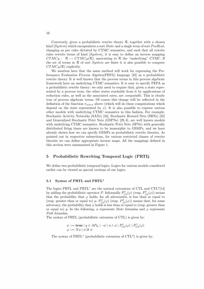
Conversely, given a probabilistic rewrite theory R, together with a chosenkind [System] which encapsulates a sort State and a single term of sort PosReal,changing as per rules dictated by CTMC semantics, and such that all rewriterules rewrite terms of kind [System], it is easy to define an inverse mappingCTMCR : R 7→ CTMCR(R), associating to R the “underlying” CTMC. Ifthe set of terms in R of sort System are finite it is also possible to computeCTMCR(R) explicitly.

We mention here that the same method will work for expressing the Per-formance Evaluation Process Algebra(PEPA) language [22] as a probabilisticrewrite theory. It is well known that the process terms in this process algebraicframework have an underlying CTMC semantics. It is easy to specify PEPA asa probabilistic rewrite theory: we only need to require that, given a state repre-sented by a process term, the other states reachable from it by applications ofreduction rules, as well as the associated rates, are computable. This is clearlytrue of process algebraic terms. Of course this change will be reflected in thedefinition of the function πselect above (which will do these computations whichdepend on the state represented by x). It is also possible to express variousother models with underlying CTMC semantics in this fashion. For example,Stochastic Activity Networks (SANs) [34], Stochastic Reward Nets (SRNs) [35]and Generalized Stochastic Petri Nets (GSPNs) [29, 8], are well known modelswith underlying CTMC semantics. Stochastic Petri Nets (SPNs) with generallydistributed firing times are known to be isomorphic to GSMPs, and we havealready shown how we can specify GSMPs as probabilistic rewrite theories. Aspointed out in respective subsections, for various restricted classes of rewritetheories we can define appropriate inverse maps. All the mappings defined inthis section were summarized in Figure 1.

5 Probabilistic Rewriting Temporal Logic (PRTL)

We define two probabilistic temporal logics. Logics for various models consideredearlier can be viewed as special versions of our logics.

5.1 Syntax of PRTL and PRTL∗

The logics PRTL and PRTL∗ are the natural extensions of CTL and CTL*[14]by adding the probabilistic operator P . Informally P ∀≤p(ϕ) (resp. P ∀≥p(ϕ)) meansthat the probability that ϕ holds, for all adversaries, is less than or equal to(resp. greater than or equal to) p. P ∃≤p(ϕ) (resp. P ∃≥p(ϕ)) means that, for someadversary, the probability that ϕ holds is less than or equal to (resp. greater thanor equal to) p. In the following, φ represents State formulas and ϕ representsPath formulas.The syntax of PRTL (probabilistic extension of CTL) is given by:

φ ::= true | q ∈ APΠ | ¬φ | φ ∧ φ | P ∀./p(ϕ) | P ∃./p(ϕ)ϕ ::= Xφ | φ U φ

The syntax of PRTL∗ (probabilistic extension of CTL*) is given by:

18

such systems, the logic CSL (continuous stochastic logic) [1, 2] 6 can be seen asa special case of PRTL by removing the operator P ∃./p from PRTL. Any formulaof the form φ1 U ≤tφ2 in CSL can be expressed by a formula of the form φ′1 U φ′2in PRTL by including the atomic propositions involving the state variable t inthe state formulas φ1 and φ2.

6 Tools: The PMaude Interpreter and Other Tools

We have developed an interpreter called PMaude , which provides a frame-work for specification and execution of finitary probabilistic rewrite theories.The PMaude interpreter has been built on top of Maude 2.0 [10] using theFull-Maude library [13]. We describe below how a finitary probabilistic rewritetheory is specified in our implemented framework and discuss some of the im-plementation details.

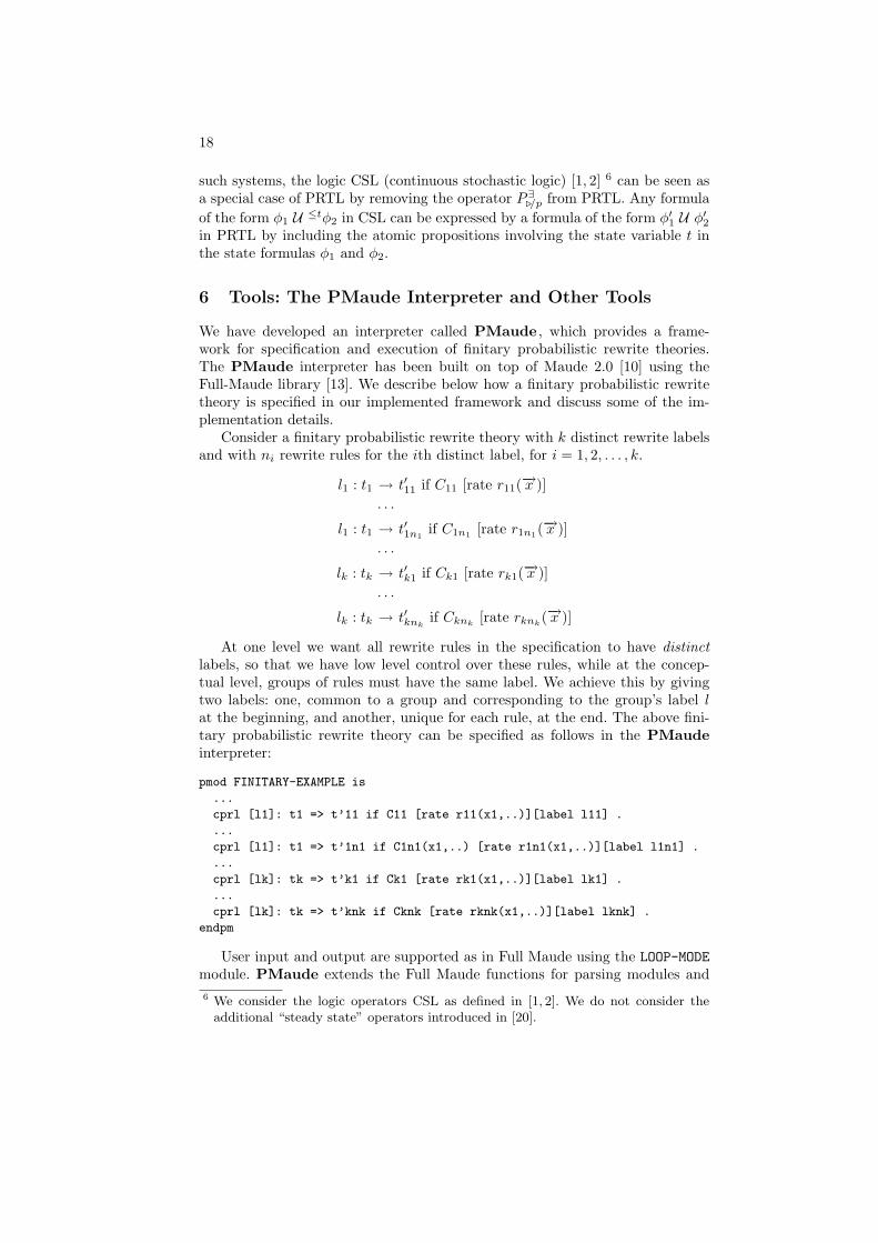
Consider a finitary probabilistic rewrite theory with k distinct rewrite labelsand with ni rewrite rules for the ith distinct label, for i = 1, 2, . . . , k.

l1 : t1 → t′11 if C11 [rate r11(−→x )]· · ·

l1 : t1 → t′1n1if C1n1 [rate r1n1(

−→x )]· · ·

lk : tk → t′k1 if Ck1 [rate rk1(−→x )]· · ·

lk : tk → t′knkif Cknk

[rate rknk(−→x )]

At one level we want all rewrite rules in the specification to have distinctlabels, so that we have low level control over these rules, while at the concep-tual level, groups of rules must have the same label. We achieve this by givingtwo labels: one, common to a group and corresponding to the group’s label lat the beginning, and another, unique for each rule, at the end. The above fini-tary probabilistic rewrite theory can be specified as follows in the PMaudeinterpreter:

pmod FINITARY-EXAMPLE is

...

cprl [l1]: t1 => t’11 if C11 [rate r11(x1,..)][label l11] .

...

cprl [l1]: t1 => t’1n1 if C1n1(x1,..) [rate r1n1(x1,..)][label l1n1] .

...

cprl [lk]: tk => t’k1 if Ck1 [rate rk1(x1,..)][label lk1] .

...

cprl [lk]: tk => t’knk if Cknk [rate rknk(x1,..)][label lknk] .

endpm

User input and output are supported as in Full Maude using the LOOP-MODEmodule. PMaude extends the Full Maude functions for parsing modules and6 We consider the logic operators CSL as defined in [1, 2]. We do not consider the

additional “steady state” operators introduced in [20].

19

any terms entered later by the user for rewriting purposes. Currently PMaudesupports four user commands. Two of these are low level commands used tochange certain seeds of pseudo-random generators. We shall not describe theimplementation of the two commands here. The other two commands are rewritecommands. Their syntax is as follows:

(prew t .)

(prew-[n] t .)

The default module M in which these commands are interpreted is the last readprobabilistic module. The prew command is an instruction to the interpreter torewrite the term t in the default module M, till no further rewrites are possible.Of course, it could happen that this command fails to terminate. The prew-[n]command takes a natural number n specifying the maximum number of rewritesto perform on the term t. This command always terminates in at most n stepsof rewriting. Both commands report the final term (if prew terminates).

The implementation of these commands is as follows. When the interpreteris given one of these commands, it extracts the term t from the commandand then computes all possible one-step rewrites for t in the default moduleM. Out of all possible groups l1,l2,..,lk in which some rewrite rule applies,one is chosen, uniformly at random. For the chosen group li, all the rewriterules li1,li2,..,lini associated with li, are guaranteed to have the sameleft-hand side ti(x1,x2,..). From all possible canonical (substitution, con-text) pairs ([θ]A, [C]A) for the variables xj, representing successful matches ofti(x1,x2,..) with the given term t, that is, matches that also satisfy one of theconditions Cij on the right hand side, one of the matches is chosen uniformly atrandom. This also describes the exact adversary aR ∈ A3 we associate to a givenfinitary probabilistic rewrite theory (see subsection 3.4). To choose the exactrewrite rule lij to apply, use of the rate functions is made. The values of thevarious rates rip are calculated for those rules lip such that [θ]A satisfies thecondition of the rule lip. Then these rates are normalized and the choice of therule lij is made probabilistically, based on the calculated rates. This rewrite ruleis then applied to the term t, in the chosen context with the chosen substitution.The interpreter then decides whether to stop rewriting or to proceed, based onthe command prew or prew-[n]. If the interpreter finds no successful matchesfor a given term, it immediately reports that term as the answer. Whichever waythe interpreter terminates, it always reports the final term reached. Notice thatthe rates depend on the chosen substitution. This allows users to specify verygeneral systems, in which the probabilities of actions are actually determined bythe physical state of the system. The URL for the complete code of the PMaudeinterpreter and code for two small examples are given in the Appendix.

PMaude can be used to generate execution traces of concurrent systemswith probabilistic actions. The programmer must supply the system specificationalong with the probabilities as a PMaude module and also supply a start term.The interpreter will then generate an execution trace for the system as perthe specification. To obtain different traces the seeds for the random numbergenerators must be changed at each invocation. This can be done by using ascripting language to call the interpreter repeatedly but setting different seeds

20

before each execution. The simulation traces generated by PMaude can be usedfor various purposes. They can be used to infer the average behavior of certainparameters of interest as well as for probabilistic validation of properties [39].

6.1 Extensions of PMaude and use with other tools

The scheme used to represent finitary probabilistic rewrite theories in PMaudecan be extended to also represent more general probabilistic rewrite theories.Moreover, we can implement the mappings CTMCR, PNSR and GSMPR re-spectively to convert certain restricted classes of probabilistic rewrite theoriesinto the underlying models CTMC, PNS and GSMP. In the case of PNSs andCTMCs one can use existing tools like ETMCC and PRISM [19, 27] for model-checking the initial specification. The mapping CTMCR also provides us withthe ability to use a number of other tools. These include the Stochastic Petri NetPackage (SPNP) [9] for verifying SPNs and SRNs; and the UltraSAN package[11] for verifying SANs. The GSPMR mapping enables us to use the GMSimtool [36] which has been developed to analyze GSMPs (recall Figure 1).

Finally, note that for systems such as GSMPs for which no known verificationtools exist, acceptance sampling methods have been used to provide probabilisticvalidation of properties [39]. These methods depend on simulation traces of exe-cutions. As pointed out in Section 6 the PMaude tool can be used to generatesimulation traces.

7 Conclusions and Future Work

We have developed probabilistic rewrite theories which provide a general se-mantic framework supporting high level specification of probabilistic systems.We showed how various well known models can be seen as special cases of ourgeneral framework. For one fairly general subclass, namely finitary probabilisticrewrite theories, we have implemented a simulator PMaude and tested it onsome relatively simple examples. However further work is required in developingthe theory, enhancing the tool and carrying out case studies.

On the more theoretical side, we feel that it is important to develop a generalmodel of probabilistic systems with concurrent probabilistic actions, as opposedto the current interleaving semantics. One then needs to define the semanticsof such systems and the associated probability space. Moreover, deductive andanalytic methods for property verification of probabilistic systems, based on ourcurrent framework seems to be an important research direction. As an appli-cation of our theory, we believe that it will be fruitful to apply our ideas tothe study of probabilistic hybrid systems, where, apart from time, there areother continuous state variables of interest whose stochastic behavior might beof interest.

Extending the PMaude framework to enable specification of more generalclass of probabilistic rewrite theories and adversaries is required. This will allowthe generation of simulation traces for the system under consideration and willbe necessary for implementation of the model independent Monte-Carlo simu-lation and acceptance sampling methods in [39] for our logics (see Section 5).

21

Furthermore, development of algorithms for implementation of the mappingsRPNS , RGSMP , RCTMC (see Section 4) will allow hooking up our tool withother verification and performance analysis tools [27, 20, 7, 36].

8 Acknowledgment

The work is supported in part by the Defense Advanced Research ProjectsAgency (the DARPA IPTO TASK Program, contract number F30602-00-2-0586and the DARPA IXO NEST Program, contract number F33615-01-C-1907) andthe ONR Grant N00014-02-1-0715. We would like to thank Narciso Martı-Olietand Abhay Vardhan for reading a previous version of this paper and givingus valuable feedback and Joost-Pieter Katoen for very helpful discussions andpointers to references.

References

1. A. Aziz, K. Sanwal, V. Singhal, and R. K. Brayton. Verifying continuous-timeMarkov chains. In Rajeev Alur and Thomas A. Henzinger, editors, Eighth In-ternational Conference on Computer Aided Verification CAV, volume 1102, pages269–276, New Brunswick, NJ, USA, 1996. Springer Verlag.

2. A. Aziz, K. Sanwal, V. Singhal, and R. Brayton. Model-checking continuous-timeMarkov chains. ACM Transactions on Computational Logic (TOCL), 1(1):162–170, 2000.

3. C. Baier and M. Z. Kwiatkowska. Model checking for a probabilistic branchingtime logic with fairness. Distributed Computing, 11(3):125–155, 1998.

4. J. Bergstra and J. Tucker. Characterization of computable data types by means ofa finite equational specification method. In J. W. de Bakker and J. van Leeuwen,editors, Automata, Languages and Programming, Seventh Colloquium, pages 76–90.Springer-Verlag, 1980. LNCS, Volume 81.

5. A. Bianco and L. de Alfaro. Model checking of probabilistic and nondeterministicsystems. FSTTCS: Foundations of Software Technology and Theoretical ComputerScience, 15, 1995.

6. A. Bouhoula, J.-P. Jouannaud, and J. Meseguer. Specification and proof in mem-bership equational logic. Theoretical Computer Science, 236:35–132, 2000.

7. G. Chiola, C. Anglano, J. Campos, J. M. Colom, and M. Silva. Operational analysisof timed Petri nets and application to the computation of peformance bounds. In5th International Workshop on Petri Nets and Performance Models, Toulouse (F)19.-22. October 1993, pages 128–137, 1993.

8. G. Ciardo, R. German, and C. Lindemann. A characterization of the stochasticprocess underlying a stochastic Petri net. Software Engineering, 20(7):506–515,1994.

9. G. Ciardo, J. K. Muppala, and K. S. Trivedi. SPNP: Stochastic Petri net package.In PNPM, pages 142–151, 1989.

10. M. Clavel, F. Duran, S. Eker, P. Lincoln, N. Martı-Oliet, J. Meseguer, and J. Que-sada. Maude: specification and programming in rewriting logic. Theoretical Com-puter Science, 285:187–243, 2002.

11. J. A. Couvillion, R. Freire, R. Johnson, W. D. Obal, M. A. Qureshi, M. Rai, W. H.Sanders, and J. E. Tvedt. Performability modeling with ultraSAN. IEEE Software,8(5):69–80, Sept. 1991.

22

12. L. de Alfaro. Temporal logics for the specification of performance and reliability.In Symposium on Theoretical Aspects of Computer Science, pages 165–176, 1997.

13. F. Duran and J. Meseguer. On parameterized theories and views in Full Maude2.0. In K. Futatsugi, editor, Proc. 3rd. Intl. Workshop on Rewriting Logic and itsApplications. ENTCS, Elsevier, 2000.

14. J. Edmund M. Clarke, O. Grumberg, and D. A. Peled. Model checking. MIT Press,1999.

15. L. Franken and B. Haverkort. Quality of service management using generic mod-elling and monitoring techniques distrib, 1997.

16. S. Gilmore and J. Hillston. The PEPA workbench: A tool to support a pro-cess algebra-based approach to performance modelling. In Computer PerformanceEvaluation, pages 353–368, 1994.

17. P. Glynn. The role of generalized semi-Markov processes in simulation outputanalysis, 1983.

18. P. J. Haas and G. S. Shedler. Regenerative simulation of stochastic Petri nets. InInternational Workshop on Timed Petri Nets, Torino, Italy, July 1–3, 1985, pages14–21. IEEE Computer Society Press, 1985.

19. H. Hermanns, J. Katoen, J. Meyer-Keyser, and M. Siegle. A Markov chain modelchecker. Tools and Algorithms for the Construction and Analysis of Systems, 6thInternational Conference, TACAS 2000,Berlin, Germany, pages 347 – 362, 2000.

20. H. Hermanns, J.-P. Katoen, J. Meyer-Kayser, and M. Siegle. A Markov chainmodel checker. In Tools and Algorithms for Construction and Analysis of Systems,pages 347–362, 2000.

21. J. Hillston. A Compositional Approach to Performance Modelling. PhD thesis.Distinguished Dissertations Series. Cambridge University Press, 1996.

22. J. Hillston. A Compositional Approach to Performance Modelling. CambridgeUniversity Press, 1996.

23. J. Hillston and M. Ribaudo. Stochastic process algebras: A new approach to per-formance modeling. In J. W. K. Bagchi and G. Zobrist, editors, Modeling andSimulation of Advanced Computer Systems. Gordon Breach, 1998.

24. J.-P. Katoen, M. Kwiatkowska, G. Norman, and D. Parker. Faster and symbolicCTMC model checking. Lecture Notes in Computer Science, 2165, 2001.

25. N. Kumar, K. Sen, J. Meseguer, and G. Agha. Probabilistic rewrite theories.manuscript, June 2002. http://yangtze.cs.uiuc.edu/∼ksen/papers/prwth.ps.

26. M. Kwiatkowska, G. Norman, and J. Sproston. Probabilistic model checking of theIEEE 802.11 wireless local area network protocol. In H. Hermanns and R. Segala,editors, Proc. 2nd Joint International Workshop on Process Algebra and Proba-bilistic Methods, Performance Modeling and Verification (PAPM/PROBMIV’02),volume 2399 of LNCS, pages 169–187. Springer, 2002.

27. M. Z. Kwiatkowska, G. Norman, and D. Parker. Prism: Probabilistic symbolicmodel checker, 2002.

28. M. A. Marsan. Stochastic Petri nets: An elementary introduction. Lecture Notes inComputer Science; Advances in Petri Nets 1989, 424:1–29, 1990. NewsletterInfo:36.

29. M. A. Marsan, G. Balbo, G. Chiola, G. Conte, S. Donatelli, and G. Franceschi-nis. An introduction to generalized stochastic Petri nets. Microelectronics andReliability, 31(4):699–725, 1991.

30. M. A. Marsan, A. Bobbio, and S. Donatelli. Petri nets in performance analysis: Anintroduction. Lecture Notes in Computer Science: Lectures on Petri Nets I: BasicModels, 1491:211–256, 1998.

31. J. Meseguer. Conditional rewriting logic as a unified model of concurrency. Theo-retical Computer Science, 96(1):73–155, 1992.

23

32. J. Meseguer. Membership algebra as a logical framework for equational specifi-cation. In F. Parisi-Presicce, ed., Proc. WADT’97, 18–61, Springer LNCS 1376,1998.

33. J. Meseguer. Research directions in rewriting logic. In U. Berger and H. Schwicht-enberg, editors, Computational Logic, NATO Advanced Study Institute, Markto-berdorf, Germany, July 29 – August 6, 1997. Springer-Verlag, 1999.

34. J. F. Meyer, A. Movaghar, and W. H. Sanders. Stochastic activity networks:Structure, behavior and application. In International Workshop on Timed PetriNets, Torino, Italy, Jul. 1-3, 1985, pages 106–115. IEEE Computer Society Press,1985.

35. J. K. Muppala, G. Ciardo, and K. S. Trivedi. Stochastic reward nets for reliabil-ity prediction. Communications in Reliability, Maintenability and Serviceability,1(2):9–20, July 1994.

36. F. Nilsen. Gmsim: A tool for compositional gsmp modeling, 1998.37. P. C. Olveczky and J. Meseguer. Specification of real-time and hybrid systems in

rewriting logic. Theoretical Computer Science, 285:359–405, 2002.38. P. Viry. Equational rules for rewriting logic. Theoretical Computer Science,

285:487–517, 2002.39. H. L. S. Younes and R. G. Simmons. Probabilistic verification of discrete event

systems using acceptance sampling. In E. Brinksma and K. G. Larsen, editors,Proceedings of the 14th International Conference on Computer Aided Verification,volume 2404 of Lecture Notes in Computer Science, pages 223–235, Copenhagen,Denmark, July 2002. Springer.

Appendix

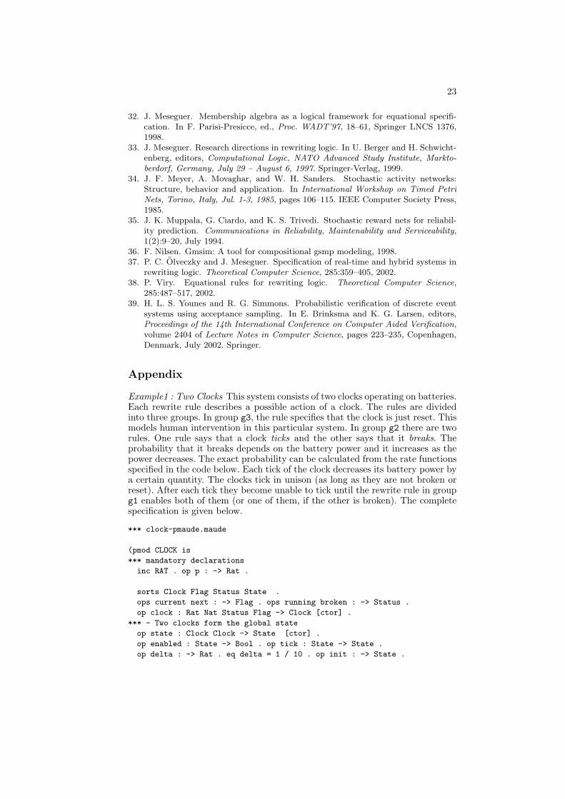
Example1 : Two Clocks This system consists of two clocks operating on batteries.Each rewrite rule describes a possible action of a clock. The rules are dividedinto three groups. In group g3, the rule specifies that the clock is just reset. Thismodels human intervention in this particular system. In group g2 there are tworules. One rule says that a clock ticks and the other says that it breaks. Theprobability that it breaks depends on the battery power and it increases as thepower decreases. The exact probability can be calculated from the rate functionsspecified in the code below. Each tick of the clock decreases its battery power bya certain quantity. The clocks tick in unison (as long as they are not broken orreset). After each tick they become unable to tick until the rewrite rule in groupg1 enables both of them (or one of them, if the other is broken). The completespecification is given below.

*** clock-pmaude.maude

(pmod CLOCK is

*** mandatory declarations

inc RAT . op p : -> Rat .

sorts Clock Flag Status State .

ops current next : -> Flag . ops running broken : -> Status .

op clock : Rat Nat Status Flag -> Clock [ctor] .

*** - Two clocks form the global state

op state : Clock Clock -> State [ctor] .

op enabled : State -> Bool . op tick : State -> State .

op delta : -> Rat . eq delta = 1 / 10 . op init : -> State .

24

var S : State . vars t t1 t2 : Nat . vars B B1 B2 : Rat .

vars f f1 f2 : Flag . vars C1 C2 : Clock . var s : Status .

*** - Definition of the enabled predicate

eq enabled( state(clock(B,t,running,current ), C2 ) ) = true .

eq enabled( state(C1,clock(B,t,running,current )) ) = true .

*** - Once a clock is broken it is never to be ticked

*** - This statement will ensure that

eq enabled(state(clock(B1,t1,broken,f1),clock(B2,t2,broken,f2)))

= true .

op enable : Clock -> Clock .

eq tick(state(C1,C2))=state(enable(C1),enable(C2)) .

eq enable (clock(B,t,running,next))=clock(B,t,running,current) .

eq enable (clock(B,t,broken,f)) = clock(B,t,broken,f) .

cprl [g1] : S => tick(S)

if enabled(S) =/= true rate[1][label tick] .

prl [g2] : clock(B,t,running,current)

=> clock(B - delta,t + 1,running,next) rate[B][label internal-run] .


=> clock(B,t,broken,current) rate[1][label internal-break] .


=> clock(B,0,running,next) rate[1][label reset] .

eq init = state(clock(100,7,running,current),

clock(200,0,running,current) ) . endpm)

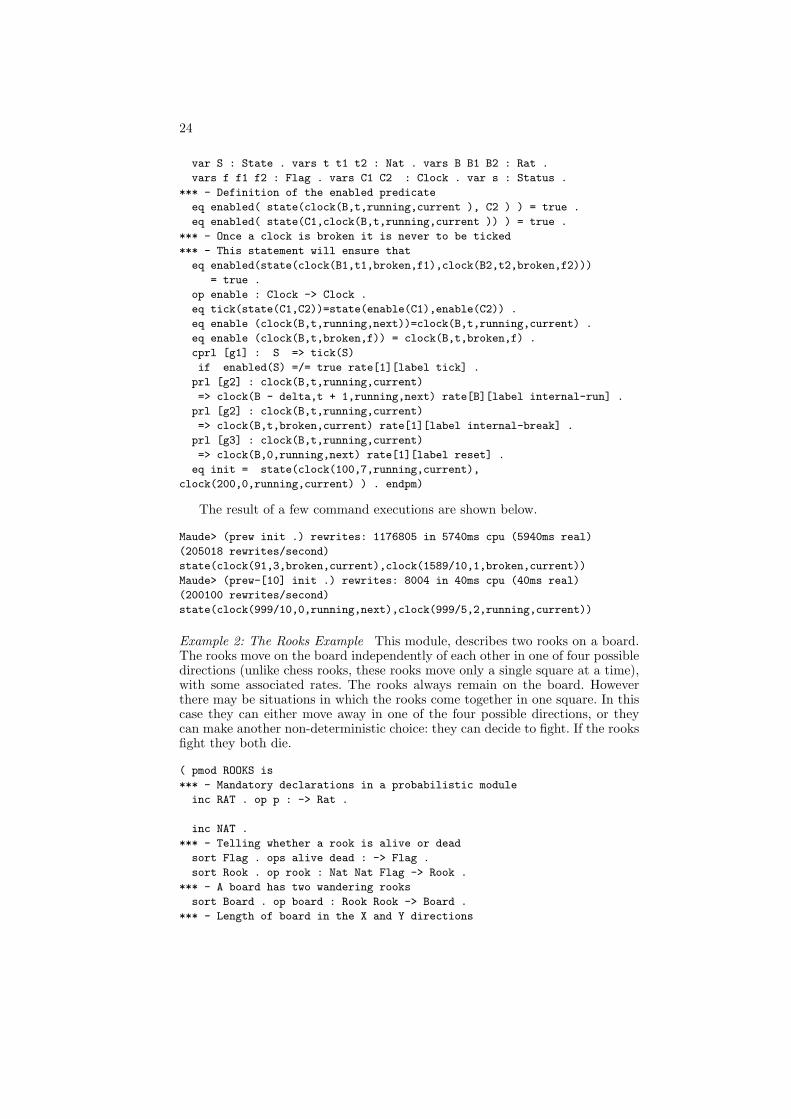
The result of a few command executions are shown below.

Maude> (prew init .) rewrites: 1176805 in 5740ms cpu (5940ms real)

(205018 rewrites/second)

state(clock(91,3,broken,current),clock(1589/10,1,broken,current))

Maude> (prew-[10] init .) rewrites: 8004 in 40ms cpu (40ms real)

(200100 rewrites/second)

state(clock(999/10,0,running,next),clock(999/5,2,running,current))

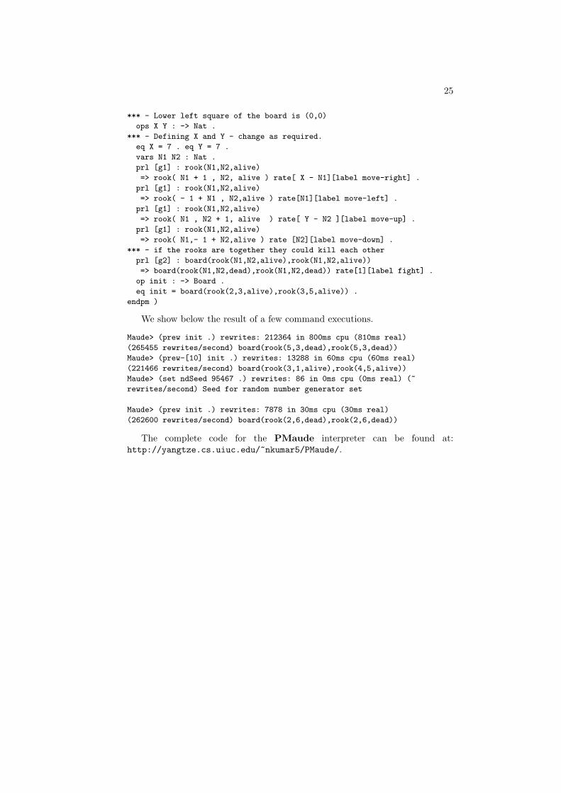
Example 2: The Rooks Example This module, describes two rooks on a board.The rooks move on the board independently of each other in one of four possibledirections (unlike chess rooks, these rooks move only a single square at a time),with some associated rates. The rooks always remain on the board. Howeverthere may be situations in which the rooks come together in one square. In thiscase they can either move away in one of the four possible directions, or theycan make another non-deterministic choice: they can decide to fight. If the rooksfight they both die.

( pmod ROOKS is

*** - Mandatory declarations in a probabilistic module

inc RAT . op p : -> Rat .

inc NAT .

*** - Telling whether a rook is alive or dead

sort Flag . ops alive dead : -> Flag .

sort Rook . op rook : Nat Nat Flag -> Rook .

*** - A board has two wandering rooks

sort Board . op board : Rook Rook -> Board .

*** - Length of board in the X and Y directions

25

*** - Lower left square of the board is (0,0)

ops X Y : -> Nat .

*** - Defining X and Y - change as required.

eq X = 7 . eq Y = 7 .

vars N1 N2 : Nat .

prl [g1] : rook(N1,N2,alive)

=> rook( N1 + 1 , N2, alive ) rate[ X - N1][label move-right] .


=> rook( - 1 + N1 , N2,alive ) rate[N1][label move-left] .


=> rook( N1 , N2 + 1, alive ) rate[ Y - N2 ][label move-up] .


=> rook( N1,- 1 + N2,alive ) rate [N2][label move-down] .

*** - if the rooks are together they could kill each other

prl [g2] : board(rook(N1,N2,alive),rook(N1,N2,alive))

=> board(rook(N1,N2,dead),rook(N1,N2,dead)) rate[1][label fight] .

op init : -> Board .

eq init = board(rook(2,3,alive),rook(3,5,alive)) .

endpm )

We show below the result of a few command executions.


(265455 rewrites/second) board(rook(5,3,dead),rook(5,3,dead))

Maude> (prew-[10] init .) rewrites: 13288 in 60ms cpu (60ms real)

(221466 rewrites/second) board(rook(3,1,alive),rook(4,5,alive))

Maude> (set ndSeed 95467 .) rewrites: 86 in 0ms cpu (0ms real) (~

rewrites/second) Seed for random number generator set


(262600 rewrites/second) board(rook(2,6,dead),rook(2,6,dead))

The complete code for the PMaude interpreter can be found at:http://yangtze.cs.uiuc.edu/~nkumar5/PMaude/.

probabilistic rewrite theories: unifying models, logics ... · probabilistic rewrite theories:...

Documents