probabilities and polarity biases in conditional … · · 2008-02-28probabilities and polarity...
TRANSCRIPT
Journal of Experimental Psychology: Copyright 2000 by the American Psychological Association, Inc. l.,eaming, Memory, and Cognition 0278-7393/00/$5.00 DOI: 10.1037//0278-7393.26.4.883 2000, Vol. 26, No. 4, 883--899
Probabilities and Polarity Biases in Conditional Inference
Mike Oaksford Cardiff University
Nick Chater and Joanne Larkin University of Warwick
A probabilistic computational level model of conditional inference is proposed that can explain polarity biases in conditional inference (e.g., J. St.B.T. Evans, 1993). These biases are observed when J. St.B.T. Evans's (1972) negations paradigm is used in the conditional inference task. The model assumes that negations define higher probability categories than their affirmative counterparts (M. Oaksfurd & K. Stenning, 1992); for example, P(not-dog) > P(dog). This identification suggests that polarity biases are really a rational effect of high-probability categories. Three experiments revealed that, consistent with this probabilistic account, when high-probability categories are used instead of negations, a high- probability conclusion effect is observed. The relationships between the probabilistic model and other phenomena and other theories in conditional reasoning are discussed.
In two areas of logical reasoning, Wason's selection task (Chater & Oaksford, 1999a; Oaksford & Chater, 1994, 1996, 1998a) and syllogistic reasoning (Chater & Oaksford, 1999b), we have argued that many of the systematic biases seen in people's inferential behavior are a result of their applying everyday prob- abilistic reasoning strategies to these laboratory tasks. That is, people are applying strategies that are normally adaptive in the uncertain world in which they live (Oaksford & Chater, 1998b). According to this view, people are not trying and falling to perform logical inferences, rather, they are succeeding in drawing proba- bilistic inferences. In this article, we present experiments showing that a similar strategy may be able to account for polarity biases in the conditional inference paradigm (e.g., Evans, 1977; Evans, Clibbens, & Rood, 1995; Kern, Mirels, & Hinshaw, 1983; Marcus & Rips, 1979; Markovits, 1988; Rumain, Connell, & Braine, 1983; Taplin, 1971; Taplin & Staudenmayer, 1973; Wildman & Fletcher, 1977).
In a conditional inference task, participants are presented with a conditional sentence such as i f a bird is a raven (p), then it is black (q) (the conditional premise) and various facts relating to the antecedent (p) and consequent (q) of the sentence (the categorical premise). From these pairs of premises, logic dictates that various
Mike Oaksford, School of Psychology, Cardiff University, Wales, United Kingdom; Nick Chater and Joanne Larkin, Department of Psychol- ogy, University of Warwick, Coventry, United Kingdom.
The experiments were conducted while Mike Oaksford was at the Department of Psychology, University of Warwick, Coventry, and Nick Chater was at the Department of Experimental Psychology, University of Oxford.
We gratefully acknowledge support of this research by the Economic and Social Research Council of the United Kingdom (Grant R000221590). We also thank Denise Cummins and two anonymous reviewers for their very helpful comments on this article.
Correspondence concerning this article should be addressed to Mike Oaksford, School of Psychology, Cardiff University, P.O. Box 901, Cardiff, CFI 3YG, Wales, United Kingdom. Electronic mall may be sent to oaksford @ cardiff.ac.uk.
883
inferences should be made or withheld. Therefore, from this rule and the fact that Tweety is a raven, it should be inferred that Tweety is black (logically this is called "modus ponens" [MP]). Logic also says that from this rule and the fact that Tweety is not black, it should be inferred that Tweety is not a raven (logically this is called "modus tollens" [MT]). Logically one cannot infer anything else. However, people are far more willing to make the MP inference than the MT inference, even though there is no logical reason to do so. Moreover, people are also willing to endorse logical fallacies such as inferring that Tweety is not black from the fact that Tweety is not a raven (this is called the fallacy of "denying the antecedent" IDA]) and that Tweety is a raven from the fact that Tweety is black (this is called the fallacy of"affLrming the consequent" [AC]). The fallacies are endorsed less often than both logical inferences, but logically they should not occur at all.
Polarity biases are observed when Evans's negations paradigm is used (Evans, 1977, 1993; Evans et al., 1995; Evans & Handley, 1999; Evans, Newstead, & Byrne, 1993; Pollard & Evans, 1980; Wildman & Fletcher, 1977). This involves incorporating negations in the antecedents and consequents of the rules to create four different task rules (A = affmnative; N = negative): i f p then q (AA); i f p then not-q (AN); i f not-p then q (NA); and i f not-p then not-q (NN; Evans & Lynch, 1973). This manipulation means that half of the conclusions of any inference--MP, DA, AC, or M T - - will be affh'mative, and half of them will be negative (i.e., the conclusion will contain a negation). Negative conclusion bias is observed when participants endorse more inferences with a nega- tive conclusion than those with an affirmative conclusion. For example, in a meta-analysis of the studies cited previously, DA was endorsed by only 45.74% of participants when the conclusion was positive, (i.e., for AN and NN; a DA conclusion negates the consequent that for these rules is not-q, and not-not-q is equivalent to q). However, DA was endorsed by 69.83% of participants when the conclusion was negative (i.e., for A_A and NA). Similarly, half of the categorical premises of any inference will be affirmative, and half will be negative. Evans (1993) argued that the mental models theory predicts an affirmative premise bias. This occurs if participants endorse more inferences with affirmative categorical
884 OAKSFORD, CHATER, AND LARKIN
premises than with negative categorical premises. Evans et al.'s (1995) experiments revealed a negative conclusion bias but no affirmative premise bias. They also showed that negative conclu- sion bias was most prevalent for DA and MT. However, Evans and Handley (1999) seem to show that negative conclusion bias is removed by the use of implicit negations--in which, for example, the categorical premise not-A is represented as K--and is replaced by an affirmative premise bias. We discuss these issues in the sequel.
Several authors have suggested that human conditional infer- ence has a significant probabilistic component (Anderson, 1995; Chan& Chua, 1994; George, 1997; Liu, Lo, & Wu, 1996; Steven- son & Over, 1995). In this article, we develop this idea by proposing a probabilistic account of polarity biases. We first develop a probabilistic computational level model (Marr, 1982) of the inferences that people should make in the conditional inference task, and we show how it may explain negative conclusion bias. We then test the main predictions of this model in three experiments.
A Conditional Probability Model of Conditional Inference
In this section, we present a model of conditional inference based on conditional probability. Anderson (1995) suggested a similar account.
Our account of polarity biases relies on Oaksford and Stenning's (1992) account in which identifying contrast sets is one important function of negations. For example, the interpretation of Johnny didn' t serve coffee (where "coffee" is the focus) is that he served a drink other than coffee. The superordinate category "drinks" provides the universe of discourse and the contrast set is defined by the operation of set difference (i.e., it is the set of "drinks Johnny could serve, less coffee"). This account is called the "otherness" theory of negation, which goes back to Plato (see also Apostel, 1972; Horn, 1989; Ryle, 1929). The set of "drinks less coffee" is likely to be much larger than the set of "coffee drinks." Consequently, Oaksford and Chater (1994) suggested that negated categories are treated as high-probability contrast sets (higher at least than their unnegated counterparts). The following equiva- lences were therefore suggested for the rules in the conditional inference task: i f p, then q <:~ LL; i f p, then not-q <:~ LH; i f not-p, then q ¢:) HL; i f not-p, then not-q ¢:~ H H (H = high, L = low, the pair, e.g., HL, is ordered to indicate a high P(p) and low P(q) rule). These equivalences allow polarity biases to be reinterpreted. Neg- ative conclusion bias can be regarded as a preference for high- probability conclusions, and affirmative premise bias can be re- garded as a preference for low-probability (categorical) premises.
Our account of how negations influence conditional inference is not a complete explanation of how people deal with negations. Negations can perform many different communicative functions: They allow us to refuse, to lie, to be ironic, to deny presupposi- tions, to distinguish truth from falsity (Horn, 1989) as well as to identify contrast sets. Our contention is that in the experiments on polarity biases, which typically use informationally impoverished abstract material, enough participants attend to a negations role in identifying contrast sets to explain these polarity preferences that are seen in the aggregate data. We argue that these preferences may be rational given a probabilistic model of conditional inference.
A Computational Level Model
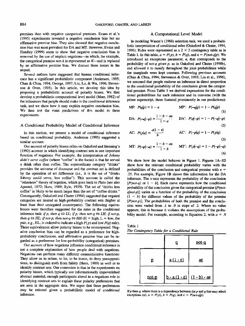
In modeling Wason's (1968) selection task, we used a probabi- listic interpretation of conditional rules (Oaksford & Chater, 1994, 1996). Rules were represented as a 2 × 2 contingency table as in Table 1. In this table, a = P(p), b = P(q), and • = P(not-qLo). We introduced an exceptions parameter, •, that corresponds to the probability of not-q given p, as in Oaksford and Chater (1998b), and allowed it to ramify throughout the joint probabilities while the marginals were kept constant. Following previous accounts (Chan & Chua, 1994; Stevenson & Over, 1995; Liu et al., 1996), we assumed that people endorse an inference in direct proportion to the conditional probability of the conclusion given the categor- ical premise. From Table 1 we derived expressions for the condi- tional probabilities for each inference and its converse (with the prime superscript, these featured prominently in our predictions):
MP: P(q~) = 1 - E NIP': P(--q~) = 1 - P(q~) (1)
1 - b - a ~ DA: p(--,ql---~p) = 1 - a DA': P(qI-"P) = 1 - P(--,ql--~p)
(2)
A C : e(Plq) = a(1 - ~) AC': e ( - -g ' l q ) = 1 - P(Plq) b
(3) 1 - b - a •
MT: P(--Pl"q) = 1 - b MT': P(PI-'q) = 1 - P(-'~l"q)
(4)
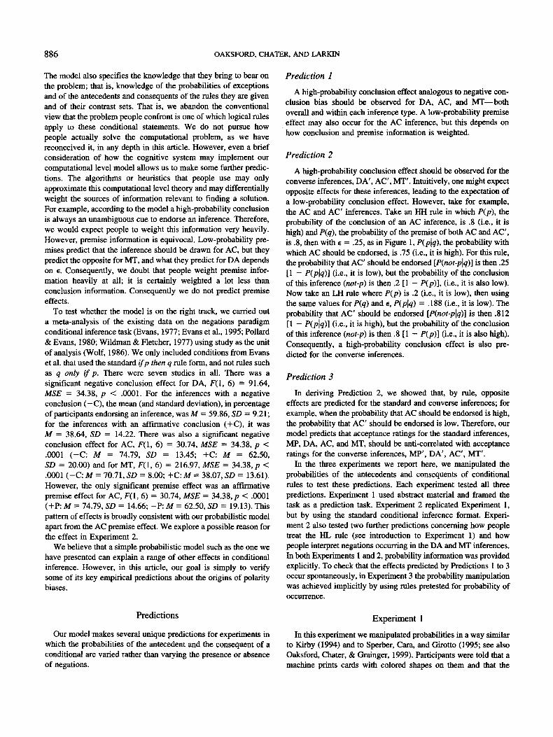
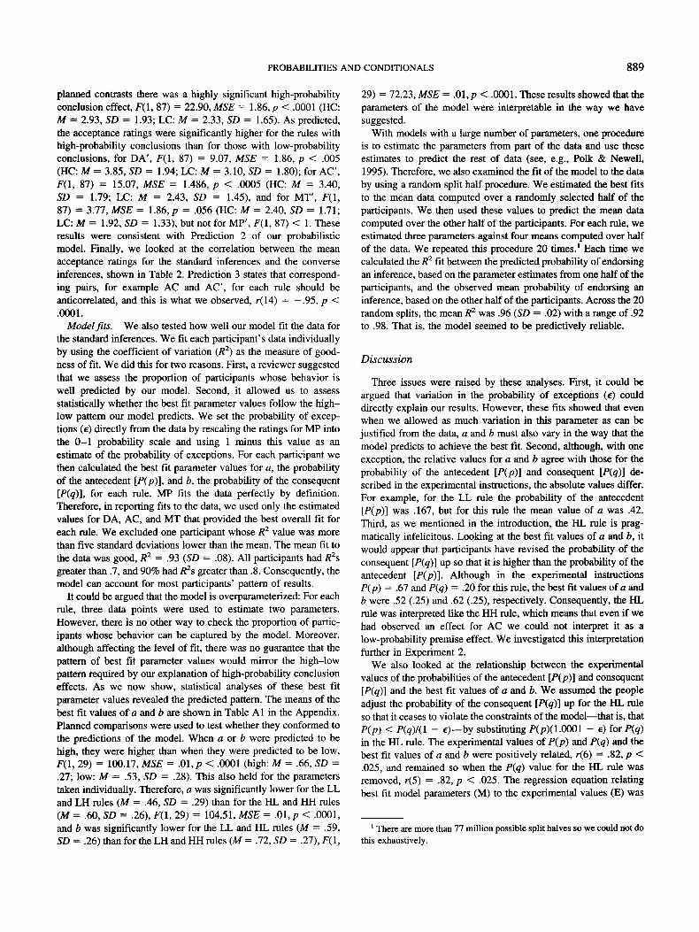
We show how the model behaves in Figure 1. Figures 1A-1D show how the relevant conditional probability varies with the probabilities of the conclusion and categorical premise with ~ = .25. For example, Figure 1B shows this information for the DA inference. The x-axis represents the probability of the conclusion [P(not-q) or 1 - b]. Each curve represents how the conditional probability of the conclusion given the categorical premise [P(not- qlnot-p)] varies as a function of the probability of the conclusion (1 - b) for different values of the probability of the premise [P(not-p)]. The probabilities of both the premise and the conclu- sion were varied from .1 to .9 in steps of .2. Where no value appears, this is because it violates the assumptions of the proba- bility model. For example, according to Equation 2, with a = .9
Table 1 The Contingency Table f o r a Conditional Rule
g
12 a (1 - E)
not -p b - a ( 1 - e)
not-q
ag
(1 - b) - ae
Ifp then q, where there is a dependency between thep and q that may admit exceptions (8). a = P(p), b = P(q), and ~ = P(not-q~).

A 1
0.75 -
e~ ~- 0 . 5 - t3.
0.25 -
0
B i -
I I I I I
0.1 0.3 0.5 0.7 0.9
P(not-qlp)
.75 -
o
,o" 0.5 -
o_ 0.25 -
I I I I I
0.1 0.3 0.5 0.7 0.9
1 - b
PROBABILITIES AND CONDITIONALS 885
C l D 1 -
Z .75 0 . 7 5 -
o - 8
0 5 0 5 o . o
0.25 % . 2 5
0 i I I I I 0 I i i I I
0.1 0.3 0.5 0.7 0.9 0.1 0.3 0.5 0.7 0.9
a 1-a
.1 [] .5 O
P(Premise) .3 I .7 i m I w
.9 A
Figure 1. How the probability that a conclusion should be drawn varies as a function of the probability of the premise and conclusion for DA (Panel B), for AC (Panel C) and for MT (Panel D). The probability that an MP (Panel A) inference should be drawn relies only on the exceptions parameter e (P[not-q~]).
(so the probability of the premise is .1), with b = .5 (so the probability of the conclusion is also .5), and with e = .25, the conditional probability of the conclusion given the categorical premise [P(not-qInot-p)] is 2.75 (i.e., it is not in the 0-1 probability interval). As the probability of the conclusion of DA, AC, or MT increases, the probability that any of these inferences will be drawn also increases. This is consistent with a high-probability conclu- sion effect. This relationship holds for all three inferences as long as there are exceptions. If there are no exceptions, then the prob- ability of drawing an MT inference [P(not-p]not-q)] is equal to 1 and therefore MT should be drawn regardless of the probability of the premise or conclusion. The exceptions parameter (e) is 1 - P(qkT), which is why MP [P(qLa)] only relies on this single pa- rameter. Linguistically the structure o f / f . . , then rules reflects the
causal ordering of events in the world (Comrie, 1986) which allow us to predict what will happen next. These predictions only go awry because of exceptions. Thus, MP and the reasons why it might fail are particularly eognitively salient (Cummins, Lubart, Alksnis, & Rist, 1991), which is why we treat exceptions as a primitive parameter of the model.
A low-probability premise effect is predicted for AC and also for DA when the probability of the conclusion (1 - b) is greater than E (see Figure 1A), but the opposite effect is predicted for MT (see Figure 1, Panel D). Consequently, a low-probability premise effect is only unequivocally predicted for the AC inference.
This model is defined at Marr's (1982) computational level; that is, it outlines the computational problem people are attempting to solve when they are given conditional inference tasks to perform.
886 OAKSFORD, CHATER, AND LARKIN
The model also specifies the knowledge that they bring to bear on the problem; that is, knowledge of the probabilities of exceptions and of the antecedents and consequents of the rules they are given and of their contrast sets. That is, we abandon the conventional view that the problem people confront is one of which logical rules apply to these conditional statements. We do not pursue how people actually solve the computational problem, as we have reconceived it, in any depth in this article. However, even a brief consideration of how the cognitive system may implement our computational level model allows us to make some further predic- tions. The algorithms or heuristics that people use may only approximate this computational level theory and may differentially weight the sources of information relevant to finding a solution. For example, according to the model a high-probability conclusion is always an unambiguous cue to endorse an inference. Therefore, we would expect people to weight this information very heavily. However, premise information is equivocal. Low-probability pre- mises predict that the inference should be drawn for AC, but they predict the opposite for MT, and what they predict for DA depends on e. Consequently, we doubt that people weight premise infor- marion heavily at all; it is certainly weighted a lot less than conclusion information. Consequently we do not predict premise effects.
To test whether the model is on the right track, we carried out a meta-analysis of the existing data on the negations paradigm conditional inference task (Evans, 1977; Evans et al., 1995; Pollard & Evans, 1980; Wildman & Fletcher, 1977) using study as the unit of analysis (Wolf, 1986). We only included conditions from Evans et al. that used the standard ifp then q rule form, and not roles such as q only if p. There were seven studies in all. There was a significant negative conclusion effect for DA, F(1, 6) = 91.64, MSE = 34.38, p < .0001. For the inferences with a negative conclusion ( -C) , the mean (and standard deviation), in percentage of participants endorsing an inference, was M = 59.86, SD = 9.21; for the inferences with an affirmative conclusion (+C), it was M = 38.64, SD = 14.22. There was also a significant negative conclusion effect for AC, F(1, 6) = 30.74, MSE = 34.38, p < .0001 ( - C : M = 74.79, SD = 13.45; +C: M = 62.50, SD = 20.00) and for MT, F(1, 6) = 216.97, MSE = 34.38, p < .0001 ( - C : M = 70.71, SD = 8.00; +C: M = 38.07, SD = 13.61). However, the only significant premise effect was an affh-mative premise effect for AC, F(1, 6) = 30.74, MSE = 34.38, p < .0001 (+P: M = 74.79, SD = 14.66; - P : M = 62.50, SD = 19.13). This pattern of effects is broadly consistent with our probabilistic model apart from the AC premise effect. We explore a possible reason for the effect in Experiment 2.
We believe that a simple probabilistic model such as the one we have presented can explain a range of other effects in conditional inference. However, in this article, our goal is simply to verify some of its key empirical predictions about the origins of polarity biases.
Prediction 1
A high-probability conclusion effect analogous to negative con- clusion bias should be observed for DA, AC, and MT--bo th overall and within each inference type. A low-probability premise effect may also occur for the AC inference, but this depends on how conclusion and premise information is weighted.
Prediction 2
A high-probability conclusion effect should be observed for the converse inferences, DA', AC', MT'. Intuitively, one might expect opposite effects for these inferences, leading to the expectation of a low-probability conclusion effect. However, take for example, the AC and AC' inferences. Take an HH rule in which P(p), the probability of the conclusion of an AC inference, is .8 (i.e., it is high) and P(q), the probability of the premise of both AC and AC', is .8, then with e = .25, as in Figure 1, P(plq), the probability with which AC should be endorsed, is .75 (i.e., it is high). For this rule, the probability that AC' should be endorsed [P(not-plq)] is then .25 [1 - P(p[q)] (i.e., it is low), but the probability of the conclusion of this inference (not-p) is then .2 [1 - P(p)], (i.e., it is also low). Now take an LH rule where P(p) is .2 (i.e., it is low), then using the same values for P(q) and e, P(plq) = .188 (i.e., it is low). The probability that AC' should be endorsed [P(not-plq)] is then .812 [1 - P(plq)] (i.e., it is high), but the probability of the conclusion of this inference (not-p) is then .8 [1 - P(p)] (i.e., it is also high). Consequently, a high-probability conclusion effect is also pre- dicted for the converse inferences.
Prediction 3
In deriving Prediction 2, we showed that, by rule, opposite effects are predicted for the standard and converse inferences; for example, when the probability that AC should be endorsed is high, the probability that AC' should be endorsed is low. Therefore, our model predicts that acceptance ratings for the standard inferences, MP, DA, AC, and MT, should be anti-correlated with acceptance ratings for the converse inferences, MP', DA', AC', MT'.
In the three experiments we report here, we manipulated the probabilities of the antecedents and consequents of conditional rules to test these predictions. Each experiment tested all three predictions. Experiment 1 used abstract material and framed the task as a prediction task. Experiment 2 replicated Experiment 1, but by using the standard conditional inference format. Experi- ment 2 also tested two further predictions concerning how people treat the I-IL rule (see introduction to Experiment 1) and how people interpret negations occurring in the DA and MT inferences. In both Experiments 1 and 2, probability information was provided explicitly. To check that the effects predicted by Predictions 1 to 3 occur spontaneously, in Experiment 3 the probability manipulation was achieved implicitly by using roles pretested for probability of occurrence.
Predict ions
Our model makes several unique predictions for experiments in which the probabilities of the antecedent and the consequent of a conditional are varied rather than varying the presence or absence of negations.
Exper iment 1
In this experiment we manipulated probabilities in a way similar to Kirby (1994) and to Sperber, Cara, and Girotto (1995; see also Oaksford, Chater, & Grainger, 1999). Participants were told that a machine prints cards with colored shapes on them and that the
PROBABILITIES AND CONDITIONALS 887
quality controllers believe that there is a fault. The fault is always the topic of the rule. It was imlxn'tant to make the abstract category structures similar to real-world categories. For example, i f some- one is told that "she was not driving a Mercedes," then they are likely to infer that she was driving some other make of car (e.g., a Ford, a Rover, a BMW, a Volvo, and so on). In defining task rules relating shapes and colors, we made it clear that there was a range of possible shapes (six) and colors (five). This reflects real-world categories better than the standard task presentation in which they could be interpreted as binary (e.g., a letter that is not-A is determinately a K).
Probabilities were introduced by using frequency formats (e.g., 10 out of 100) rather than probability formats (e.g., .1) because people are better able to utilize probabilistic information when it is introduced in this way (e.g., Gigerenzer & Hoffrage, 1995). Introducing probabilities in this way means that any con- ditional sentence relating the shapes and colors of the cards is implicitly universal. Indeed, it is more natural to describe a situ- ation in which there are, for example, no nongreen stars, by using the universal all the stars are green rather than the condit ional /f a card has a star on it, then it is green. The underlying logical form of both sentences is identical (i.e., V x [star(x) D green(x)]), so the inferences predicted by logic are the same. However, because of the greater naturalness of the universal, this construc- tion was used throughout.
We used a quality-control scenario so that we could provide unambiguous probability information without ruling out the pos- sibility of exceptions and so that we could realistically present an HL rule. The task rule always describes a fault and not the machine's normal mode of operation. A rule describing the occur- rence of a fault inherently admits exceptions. The HL rule is pragmatically infelicitous (Oaksford, 1998; Oaksford &Chate r , 1994; Oaksford et al., 1999). For example, it is like asserting that i f something is black it is a raven, which is known to be false. We suggested that, in Wason's selection task, to make sense of being asked to test a rule known to be false, people revise the probability of the antecedent [P(p)] down, treating it as an LL rule (Oaksford &Chater , 1994). This strategy provided good fits to the selection task data, In the current model, when there are no exceptions (e = 0), then the probability of the antecedent must be less than the prob- ability of the consequent [P(p) < P(q)]. However, when the probability of exceptions is greater than zero (E > 0), then the prob- ability of the consequent [P(q)] must be greater than the probability of the antecedent less the probability of exceptions [P(p) X (1 - e)]. This means that when there are few exceptions (e is low), as is normally the case, it is impossible to present an I lL rule. For example, i f the probability of the antecedent [P(p)] is high, say .6, and the probability of exceptions (e) is equal to .1, then it must be the case that the probability of the consequent [P(q)] is greater than .54. We got around this problem by using rules that describe how the quality controller believes the machine to be behaving. There- fore, participants may be told that the quality controller believes that all of the stars are green, although 60% of the cards are stars but only 10% of cards are green. This introduces an inconsistency between what the quality controller believes and the state of affairs in the world. However, it avoids the experimenter seemingly providing participants with contradictory information; that is, us- ing a rule to describe a situation in which it could not be true. In the Results section, we checked to see how people dealt with this
rule and whether they made any adjustments such as those we have suggested occur in the selection task. All the converse inferences were also included in this experiment.
M e t h o d
Participants. Thirty undergraduate psychology students from the Uni- versity of Warwick took part in this experiment. Each was paid £4.00 ($6.50) an hour to participate, and none had any prior knowledge of the conditional inference task.
Design~ The experiment was a 4 x 2 x 2 × 2 Inference (MP vs. DA vs, AC vs. MT) X Conclusion (standard vs. converse) X P(p) x P(q) completely within-subject design.
Materials. The materials consisted of a nine-pege booklet. The first page of each booklet was a general instruction page. Each of the following pages contained 4 of the 32 possible conditional inference problems. There were two pages for each of the LL, LH, HL, and HH rules. For each participant, these pages appeared in different random orders,
The instructions for the LL condition read as follows:
A machine prints colored shapes onto cards for educational p n ~ The shapes are circles, diamonds, squares, triangles, stars and crosses, and the colors are red, green, yellow, blue and orange.
The machine is supposed to print equal numbers of shapes of different colors. So, for example, out of every 60 cards printed, roughly there should be 10 of each shape, 2 of each shape being one of the different colors, making 12 cards of each color in total.
In a certain batch in which the quality controllers think they have detected a problem, they believe that:
All the triangles are blue
However, all the other shapes have the full range of colors printed on them. The machine sorts the cards into 11 bins labeled either with a shape (the "shapes bins") or a color (the "colors bins"). It sorts cards by shape or by color alternately, so if a card is sorted by shape, the next will be sorted by color, the next by shape and so on.
On each of the two pages for the LL rule, four of the conditional infereace problems were also presented. Which four appeared on each page was determined randomly. The problem format for the DA inference for the LL rule is shown as follows:
Given this problem, one of the quality controllers is trying to predict what they might find in the bins:
Assuming that all the triangles are blue, he looks at a shapes bin that is not labeled "triangles" and predicts that ff he picks a card out of this bin it will not be blue.
Please rate on a scale from one to seven how likely be is to be fight. (1 indicates that you are totally confident that he is wrong, 4 indicates that you are uncertain and 7 indicates that you are totally confident that he is correct; all other points on the scale (2, 3, 5, 6) can also be used) ....
The pages for the LH, HL, and HH rules were the same, but with the following changes to the rule and to the sentence after it (in italics):
LH: All the circles are red. Moreover, the machine is printing most of the other shapes red as well so that out of every 60 cards printed, roughly there are 10 of each shape. However, apart from the circles which are all red, 6 of each other shape are now red and only I of each other shape is of the remaining colors. This means that out of every 60 cards, 40 are red and the rest consist of one of the remaining color- shape combinations.
888 OAKSFORD, CHATER, AND LARKIN
HL: All the stars are green. Moreover, the machine is printing more stars than other shapes so that out of every 60 cards printed, roughly there are 40 stars and only 4 of each remaining shape. In fact the colors on each card are in proportion, that is, roughly 12 out of every 60 cards are of each color.
HH: All the squares are yellow. Moreover, the machine is printing more squares than other shapes and more yellow shapes than other colors. So, out of every 120 cards printed, roughly there are 80 squares and only 8 of each remaining shape; the 80 squares and 4 of each of the other shapes are yellow, making 100 yellow shapes in all. Of the remaining shapes, 1 of each is of the remaining colors.
Procedure. All participants were tested individually. The booklet was placed face down on a desk in the experimental cubicle. Participants were sat at the desk and told not to turn over the booklet until they were instructed. On turning over the booklet, the first page revealed the follow- ing instructions:
Your task is to solve the following problems on these pages. There are 32 problems and instructions are provided at each stage.
When participants finished the booklet, they were thanked for their participation and were fully debriefed about the purpose of the experiment.
Resu l t s
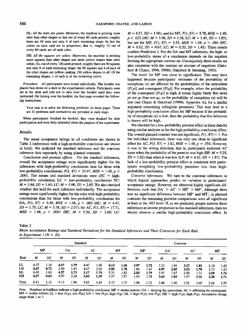
The mean acceptance ratings in all conditions are shown in Table 2 (inferences with a high-probability conclusion are shown in bold). We analyzed the standard inference and the converse inference data separately by using planned contrasts.
Conclusion and premise effects. For the standard inferences, overall the acceptance ratings were significantly nigher for the inferences with nigh-probability conclusions than for those with low-probability conclusions, F(1, 87) = 33.47, MSE = 1.48, p < .0001. The means and standard deviations were (HC = high- probability conclusion; LC = low-probability conclusion) HC: M = 5.64, SD = 1.65; LC: M = 5.00, SD = 2.05. We also checked whether this held for each inference individually. The acceptance ratings were significantly higher for the rules with high-probability conclusions than for those with low-probability conclusions for DA, F(1, 87) = 9.49, MSE = 1.48, p < .005 (HC: M = 4.47, SD = 1.75; LC: M = 3.78, SD = 2.07); for AC, F(1, 87) = 17.71, MSE = 1.48, p < .0001 (HC: M = 5.50, SD = 1.60; LC:
M = 4.57, SD = 1.98); and for MT, F(1, 87) = 5.78, MSE = 1.48, p < .025 (HC: M = 5.98, SD = 1.58, LC: M = 5.45, SD = 1.85); but not for MP, F(1, 87) = 3.53, MSE = 1.48, p = .064 (HC: M = 6.62, SD = 0.67; LC: M = 6.20, SD = 1.41). These results confirm Prediction 1. For the DA and MT inferences, the nigh- or low-probability status of a conclusion depends on the negation forming the appropriate contrast set. Consequently these results are also consistent with the contrast set account of negations (Oaks- ford & Chater, 1994, 1998b; Oaksford & Stenning, 1992).
The result for MP was close to significance. This may have happened because participants' estimates of the probability of exceptions (¢) are affected by the probabilities of the antecedent [P(p)] and consequent [P(q)]. For example, when the probability of the consequent [P(q)] is nigh, it seems highly likely that more ps are qs than not-qs, so the probability of exceptions (E) will be low (see Chater & Oaksford [1999b, Appendix A], for a similar argument concerning syllogistic premises). This may lead to a nigh-probability conclusion effect for MP because if the probabil- ity of exceptions (¢) is low, then the probability that this inference is drawn will be nigh.
We checked for a low-probability premise effect in these data by using similar analyses as for the high-probability conclusion effect. The overall planned contrast was not significant, F(1, 87) < 1. For the individual inferences, there was only one close to significant effect for AC, F(1, 87) = 3.82, MSE = 1.48, p = .054. However, it was in the wrong direction; that is, participants endorsed AC more when the probability of the premise was nigh (HP: M = 5.25, SD = 1.82) than when it was low (LP: M = 4.82, SD = 1.87). The lack of a low-probability premise effect is consistent with partic- ipants weight ing low-probabi l i ty premises less than high- probability conclusions.
Converse inferences. We turn to the converse inferences in which logical approaches predict no variation in participants' acceptance ratings. However, we observed highly significant dif- ferences, such that DA' > AC' > MT' > MP' . Although there was no significant difference between MP' and MT' , in planned contrasts the remaining pairwise comparisons were all significant at least at the .025 level. If, as we predicted, people endorse these inferences in inverse proportion to the standard inferences, then we should observe a similar nigh-probability conclusion effect. In
Table 2
Mean Acceptance Ratings and Standard Deviations f o r the Standard Inferences and Their Converses f o r Each Rule in Experiment 1 (N = 30)
Standard Converse
MP DA AC MT MP' DA' AC' MT'
Rule M SD M SD M SD M SD M SD M SD M SD M SD
LL 6.37 1.16 4.57 1.79 4.47 1.96 6.13 1.36 2.07 1.72 3.23 1.94 3.27 1.82 2.10 1.42 LH 6.67 0.71 3.50 1.87 4.67 2.02 5.83 1.78 1.80 1.65 4.07 2.05 3.53 1.78 1.73 1.23 HL 6.03 1.63 4.37 1.73 5.17 1.74 5.33 1.85 2.03 1.79 2.97 1.67 2.90 1.71 2.50 1.74 HH 6.57 0.63 4.07 2.24 5.83 1.39 5.57 1.87 1.93 1.78 3.63 1.83 1.97 0.96 2.311 1.71
Total 6.41 1.12 4.13 1.94 5.03 1.85 5.72 1.73 1.96 1.72 3.48 1.90 2.92 1.69 2.16 1.55
Note. Numbers in boldface indicate a high-probability conclusion. MP = modus ponens; DA = denying the antecedent; AC = affmnlng the consequent; MT = modus tollens; LL = low P(p), low P(q); LH = low P(p), high P(q); HL = high P(p), low P(q); HH = high P(p), high P(q). Acceptance ratings range from 1 to 7.
PROBABILITIES AND CONDITIONALS 889
planned contrasts there was a highly significant high-probability conclusion effect, F(1, 87) = 22.90, MSE = 1.86,p < .0001 (HC: M = 2.93, SD = 1.93; LC: M = 2.33, SD = 1.65). As predicted, the acceptance ratings were significantly higher for the rules with high-probability conclusions than for those with low-probability conclusions, for DA' , F(1, 87) = 9.07, MSE = 1.86, p < .005 (HC: M = 3.85, SD = 1.94; LC: M = 3.10, SD = 1.80); for AC' , F(1, 87) = 15.07, MSE = 1.486, p < .0005 (HC: M = 3.40, SD = 1.79; LC: M = 2.43, SD = 1.45), and for MT' , F(1, 87) = 3.77, MSE = 1.86, p = .056 (HC: M = 2.40, SD = 1.71; LC: M = 1.92, SD = 1.33), but not for MP', F(1, 87) < 1. These results were consistent with Prediction 2 of our probabilistic model. Finally, we looked at the correlation between the mean acceptance ratings for the standard inferences and the converse inferences, shown in Table 2. Prediction 3 states that correspond- ing pairs, for example AC and AC' , for each rule should be anticorrelated, and this is what we observed, r(14) = - .95 , p < .0001.
Modelfits. We also tested how well our model fit the data for the standard inferences. We fit each participant's data individually by using the coefficient of variation (R 2) as the measure of good- ness of fit. We did this for two reasons. First, a reviewer suggested that we assess the proportion of participants whose behavior is well predicted by our model. Second, it allowed us to assess statistically whether the best fit parameter values follow the high- low pattern our model predicts. We set the probability of excep- tions (E) directly from the data by rescaling the ratings for MP into the 0-1 probability scale and using 1 minus this value as an estimate of the probability of exceptions. For each participant we then calculated the best fit parameter values for a, the probability of the antecedent [P(p)], and b, the probability of the consequent [P(q)], for each rule. MP fits the data perfectly by definition. Therefore, in reporting fits to the data, we used only the estimated values for DA, AC, and MT that provided the best overall fit for each rule. We excluded one participant whose R 2 value was more than five standard deviations lower than the mean. The mean fit to the data was good, R 2 = .93 (SD = .08). All participants had R2s greater than .7, and 90% had R2s greater than .8. Consequently, the model can account for most participants' pattern of results.
It could be argued that the model is overparameterized: For each rule, three data points were used to estimate two parameters. However, there is no other way to check the proportion of partic- ipants whose behavior can be captured by the model. Moreover, although affecting the level of fit, there was no guarantee that the pattern of best fit parameter values would mirror the high-low pattern required by our explanation of high-probability conclusion effects. As we now show, statistical analyses of these best fit parameter values revealed the predicted pattern. The means of the best fit values of a and b are shown in Table A1 in the Appendix. Planned comparisons were used to test whether they conformed to the predictions of the model. When a or b were predicted to be high, they were higher than when they were predicted to be low, F(1, 29) = 100.17, MSE = .01,p < .0001 (high: M = .66, SD = .27; low: M = .53, SD = .28). This also held for the parameters taken individually. Therefore, a was significantly lower for the LL and LH rules (M = .46, SD = .29) than for the HL and HH rules (M = .60, SD = .26), F(1, 29) = 104.51, MSE = .01, p < .0001, and b was significantly lower for the LL and HL rules (M = .59, SD = .26) than for the LH and HH rules (M = .72, SD = .27), F(1,
29) = 72.23, MSE = .01, p < .0001. These results showed that the parameters of the model were interpretable in the way we have suggested.
With models with a large number of parameters, one procedure is to estimate the parameters from part of the data and use these estimates to predict the rest of data (see, e.g., Polk & Newell, 1995). Therefore, we also examined the fit of the model to the data by using a random split half procedure. We estimated the best fits to the mean data computed over a randomly selected half of the participants. We then used these values to predict the mean data computed over the other half of the participants. For each rule, we estimated three parameters against four means computed over half of the data. We repeated this procedure 20 times. 1 Each time we calculated the R 2 fit between the predicted probability of endorsing an inference, based on the parameter estimates from one half of the participants, and the observed mean probability of endorsing an inference, based on the other half of the participants. Across the 20 random splits, the mean R 2 was .96 (SD = .02) with a range of .92 to .98. That is, the model seemed to be predictively reliable.
Discussion
Three issues were raised by these analyses. First, it could be argued that variation in the probability of exceptions (E) could directly explain our results. However, these fits showed that even when we allowed as much variation in this parameter as can be justified from the data, a and b must also vary in the way that the model predicts to achieve the best fit. Second, although, with one exception, the relative values for a and b agree with those for the probability of the antecedent [P(p)] and consequent [P(q)] de- scribed in the experimental instructions, the absolute values differ. For example, for the LL rule the probability of the antecedent [P(p)] was .167, but for this rule the mean value of a was .42. Third, as we mentioned in the introduction, the HL rule is prag- matically infelicitous. Looking at the best fit values of a and b, it would appear that participants have revised the probability of the consequent [P(q)] up so that it is higher than the probability of the antecedent [P(p)]. Although in the experimental instructions P(p) = .67 and P(q) = .20 for this rule, the best fit values of a and b were .52 (.25) and .62 (.25), respectively. Consequently, the HL rule was interpreted like the HH rule, which means that even if we had observed an effect for AC we could not interpret it as a low-probability premise effect. We investigated this interpretation further in Experiment 2.
We also looked at the relationship between the experimental values of the probabilities of the antecedent [P(p)] and consequent [P(q)] and the best fit values of a and b. We assumed the people adjust the probability of the consequent [P(q)] up for the HL rule so that it ceases to violate the constraints of the model--that is, that P(p) < P(q)/(1 - e ) - -by substituting P(p)(1.0001 - E) for P(q) in the HL rule. The experimental values of P(p) and P(q) and the best fit values of a and b were positively related, r(6) = .82, p < .025, and remained so when the P(q) value for the HL rule was removed, r(5) = .82, p < .025. The regression equation relating best fit model parameters (M) to the experimental values (E) was
1 There ale more than 77 million possible split halves so we could not do this exhaustively.
890 OAKSFORD, CHATER, AND LARKIN
M = .43 + .32E. This suggests that there was not a perfect relationship between the experimentally provided probabilities and the value assumed when making inferences. In Experiment 3, we explored this relationship more fully and we asked participants for their individual assessments of the relevant probabilities. We also look at this relationship in more depth in the General Discussion section.
The results of Experiment 1 were consistent with most of the predictions of our probabilistic account. The use of high- and low-probability categories produced a high-probability conclusion effect, which on the contrast set account of negations (Oaksford & Stenning, 1992) is responsible for negative conclusion bias. More- over, a complementary pattern of effects was observed for the converse inferences, which is uniquely predicted by our probabi- llstic account. Furthermore, our model provided good fits to the individual data, and the model parameters were interpretable as having the high and low values required.
Experiment 2
The results of Experiment 1 supported our probabilistic model. However, there were differences between Experiment I and the standard conditional inference paradigm that may be responsible for our results. In Experiment 1, we used the universal all rather than the standard / f . . . then rule form, and the inferences were framed as prediction problems rather than in the standard condi- tional inference task format. In Experiment 2, we therefore used the i f . . . then rule form and the standard format of the task.
We also wanted to see if we could alter the pattern of inferences by manipulating the parameters of the model. Removing the pos- sibility of exceptions predicts a high-probability conclusion effect for DA and AC but not for MT. In Experiment 1, we introduced the possibility of exceptions by using rules that described faults (as in Sperber et al., 1995). In Experiment 2, we used rules that described the normal functioning of a machine and did not mention the possibility of faults, which reduced the possibility of exceptions.
The use of this manipulation meant that the HL rule could not be introduced without the experimenter seemingly providing contra- dictory information. To have the probability of the consequent, [P(q)], low for this rule is important for the DA inference that our model predicts should be endorsed strongly because the probabil- ity of the conclusion, [P(not-q)], will then be high, as will the probability that this inference is drawn [P(not-q[not-p)]. However, the best fit parameter values in Experiment 1 revealed that b > a for the HL rule. This raises the question of whether the predicted pattern of effects can occur, even though participants treat the probability of the consequent [P(q)] as greater than the probability of the antecedent [P(p)] for the HL rule. To test this, for the HL rule we set the probability of the antecedent [P(p)] to .99 and the probability of the consequent [P(q)] to .991. From Equation 2, assuming no exceptions, this means that the probability of drawing the DA inference [P(not-qlnot-p) ] is .9. Treatment of the HL rule in this way reflects the best fit parameter values found in Exper- iment 1 that suggested participants treated P(q) as greater than P(p) for this rule. Experiment 2 provided a direct test of whether the predicted conclusion and premise effects occur under this interpretation. This experiment indeed provided quite a strong test because it predicted different behavior on the DA inference for the
very similar HH rule. For this rule, we set the probability of the antecedent [P(p)] to .99 and the probability of the consequent [P(q)] to .999. Consequently, according to Equation 2 and again assuming no exceptions, the probability of drawing the DA infer- ence for this rule [P(not-qlnot-p)] is . 1. Therefore, DA should be endorsed significantly less for the HH rule than for the HL rule.
Both rules still predicted a high-probability conclusion effect for AC: For HL, from Equation 3, the probability of drawing this inference [P(PIq)] was .999; for HH, it was .991. A low- probability premise effect was also predicted for AC, because according to Equation 3, for the LL rule, the probability of drawing this inference [P(Plq)] was .5, and for LH rule it was .01. Accord- ing to the model then, the mean probability of drawing an AC inference with a low-probability premise (LL and HL) is .750, but the mean probability of drawing this inference with a high- probability premise (LH and HH) is .501. However, this prediction is mainly attributable to the HL rule, which no longer has a low-probability premise. Consequently, any low-probability premise effect we observe for AC can be explained without as- suming people are paying attention to premise information. If participants make a similar conversion for the negated antecedent rule Of not-p then q) as for the HL rule, then this would also explain the specific affirmative premise bias effect we observed for AC in our meta-analysis of the negations paradigm data.
Although reducing the possibility of exceptions may lead to more MT inferences, participants still have to process negations for this rule (and for DA). As we have discussed, Oaksford and Stenning (1992) showed that processing negations is a serious source of difficulty in conditional reasoning. However, two ma- nipulations reduce the effects of processing negations. First, Oaks- ford and Stenning have shown that binary materials make contrast set construction easier. For, example, with only two colors, say red and green, a shape that is not red is unequivocally green. Second, the use of implicit rather than explicit negations (Evans, 1983) also removes the effects of processing negations. For example, the use of implicit negations with binary materials for the rule i fA then 2 would involve presenting MT as if A then 2, 7, therefore K rather than as if A then 2, not-2, therefore not-A which is the standard explicit presentation. By combining binary materials with implicit negations we can present an MT inference without negations. If nonbinary materials were used the conclusion would still have to be presented as not-A. (We discuss the relationship between these experiments and other research using the implicit negations ma- nipulation further in the General Discussion section.)
These manipulations were predicted to affect the MT inference. With the possibility of exceptions reduced, the probability with which people should draw this inference is close to 1. Therefore, the only reason for any asymmetry with MP is the presence of negations. However, the use of implicit negations with binary material removes the need to use negations to express MT. Con- sequently, this manipulation makes two predictions. First, in an implicit condition, MT inferences should be drawn as frequently as MP inferences. Second, more MT inferences should be made in an implicit condition than in a standard explicit negations condition. A related prediction could be made for DA. However, according to our model for DA (and AC), participants must concentrate on the relative set sizes to determine how strongly to endorse an inference even if the possibility of exceptions is reduced. The removal of the negations does not prevent the need to process this information.
PROBABILITIES AND CONDITIONALS 891
Therefore , we predic ted that there wou l d be no increase in D A
ana logous to M T in an implici t nega t ions condi t ion.
In this exper iment , we therefore used rules that d id not in t roduce
the poss ibi l i ty o f except ions , we u sed b ina ry mater ia l s and we
in t roduced two condi t ions: one u s i ng expl ic i t nega t ions , and one
u s ing implici t nega t ions .
M e t h o d
Participants. Twenty-five undergraduate psychology students from the University of Warwick took part in this experiment. Each participant was paid £4.00 ($6.50) an hour to participate. None of the participants had any prior knowledge of the conditional inference task.
Design. The experiment was a 4 × 2 x 2 × 2 × 2 Inference (MP vs. DA vs. AC vs. MT) × Conclusion (standard vs. converse) × Negations (explicit vs. implici0 × P(p) × P(q) completely within-subject design.
Materials. For each participant the materials consisted of eight 9-page booklets and a single-page instruction sheet. There were two booklets for each of the rules: one in which implicit negations were used, and one in which explicit negations were used. Each booklet contained all four infer- ences and their converses. The first page of each booklet was an instruction page. For each participant, these problems appeared in different random orders in each booklet, and each booklet was presented to each participant in different random orders.
Procedure. All participants were tested individually. The instruction sheet and the first randomly assigned booklet was placed face down on a desk in the experimental cubicle. Participants were sat at the desk and told not to turn over the instruction sheet or booklet until they were told to do so. The other side of the instruction sheet revealed the following instruc- tions:
You will be presented with 8 booklets, one at a time. Please read the instructions carefully on the front of each one and call the experi- menter after you have worked through each booklet. Thank you.
The first page of each booklet contained the following instructions. The LL condition is used as an example:
A company manufactures cards for educational use with numbers on one side and letters printed on the other side.
One batch of cards uses just the letters "S" and "W," and just the numbers "5" and "8."
O n the front of 10 of the I000 cards there is an " S " and on the front of the remaining 990 cards there is a " W "
For every 1000 cards in this batch;
On the back o f the 10 "S" s there is a "5," and;
On the back o f the 990 "W" s, t 0 have a "5" and 980 have an "8. "
Consequently, the machine obeys the following rule:
I f a card has an "S" on the front, then it has a "5" on the back.
Your task on the following pages will be to evaluate some inferences about these cards. Please place a mark on the scale to indicate your answer. You may refer back to these instructions.
For the LH condition, the letters J and R and the numbers 9 and 6 were used, and the statements in italics were replaced with the following:
On the back of the 10 "J"s there is a "9," and;
On the back of the 990 "R"s, 980 have a "9" and 10 have a "6."
The rule used was
As discussed in the introduction, for the HL rule, P(q) was adjusted to just above P(p). For the HL role, the letters D and C and the numbers 4 and 1 were used. The sentence in bold was also replaced with the following sentence:
On the front of 990 of every 1000 cards there is an " D " and on the front of the remaining 10 cards there is a "C."
The statements in italics were replaced with the following:
On the back of the 990 "D"s there is a "4," and;
On the back of the 10 "C"s, 1 has a "4" and 9 have a "1."
The rule used was
If a card has a "D" on the front, then it has a "4" on the back.
The HH condition was the same as HL, but the letters A and K and the numbers 2 and 7 were used, and the statements in italics were replaced with the following:
On the back of the 990 "A"s there is a "2," and;
On the back of the 10 "K"s, 9 have a "2" and 1 has a "7."
The rule used was
If a card has a "A" on the front, then it has a "2" on the back.
On each of the following pages, participants had to rate the acceptability of a conclusion to one of the eight inference types using a rating scale as in Cummins et al. (1991). The MP inference for the LL rule is used as an example:
If a card has an S on the front, then it has a 5 on the hack.
This card has an S on the front.
Therefore this card has a 5 on the back.
Given this rule and this fact, place a mark on the scale below that best reflects your evaluation of the conclusion.
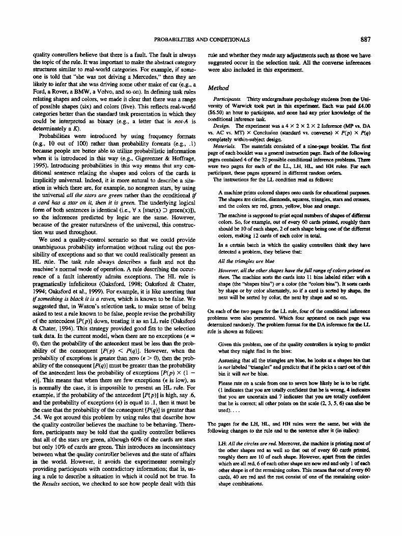
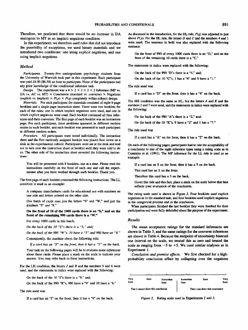
The rating scale used is shown in Figure 2. Four booklets used explicit negations as in the standard task, and four booklets used implicit negations in the categorical premise and in the conclusion.
When participants finished the last booklet they were thanked for their participation and were fully debriefed about the purpose of the experiment.
R e s u l t s
The m e a n accep tance ra t ings for the s tandard in fe rences are
s h o w n in Tab le 3, and the s a m e ra t ings for the conve r se in fe rences
are s h o w n in Table 4. B e c a u s e the midpo in t o f uncer ta in ty b isec ted
one interval on the scale, we treated this as zero and treated the
scale as r ang ing f r o m - 5 to + 5 . W e used s imi lar ana lyses as in
Expe r imen t 1.
Conclus ion and p remi se effects. W e fLrst checked for a h igh-
probabi l i ty conc lus ion effect by col laps ing over the nega t ions
f I i •
Very Sure Somewhat Somewhat Sure Very S~ Sure I Sure Sure
Thatlcannotdraw~sco~l~ I That lcandraw~is~|mkm
If a card has an "J" on the front, then it has a "9" on the back. Figure 2. Rating scale used in Experiments 2 and 3.
892 OAKSFORD, CHATER, AND LARKIN
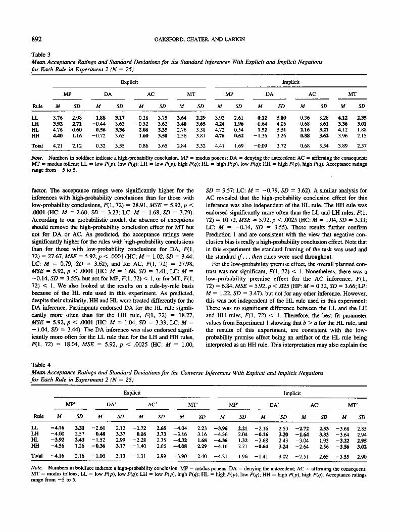
Table 3 Mean Acceptance Ratings and Standard Deviations for the Standard Inferences With Explicit and Implicit Negations for Each Rule in Experiment 2 (N = 25)
Explicit Implicit
MP DA AC MT MP DA AC MT
Rule M SD M SD M SD M SD M SD M SD M SD M SD
LL 3.76 2.98 1.88 3.17 0.28 3.75 3.64 2.29 3.92 2.61 0.12 3.80 0.36 3.28 4.12 2.35 LH 3.92 2.71 -0.44 3.63 -0.52 3.62 2.40 3.65 4.24 1.96 -0.64 4.05 -0.68 3.61 3.36 3.01 I-B., 4.76 0.60 0.56 3.36 2.08 3.35 2.76 3.38 4.72 0.54 1.52 3.31 2.16 3.21 4.12 1.88 HH 4,40 1.16 -0.72 3.65 1.60 3.50 2.56 3.81 4.76 0.52 -1.36 3.26 0.88 3.62 3.96 2.15
Total 4.21 2.12 0.32 3.55 0.86 3.65 2.84 3.32 4.41 1.69 -0.09 3.72 0.68 3.54 3.89 2.37
Note. Numbers in boldface indicate a high-probability conclusion. MP = modus ponens; DA = denying the antecedent; AC = affirming the consequent; MT = modus tollens; LL = low P(p), low P(q); LH = low P(p), high P(q); HL = high P(p), low P(q); HH = high P(p), high P(q). Acceptance ratings range from - 5 to 5.
factor. The acceptance ratings were significantly higher for the inferences with high-probability conclusions than for those with low-probability conclusions, F(1, 72) = 28.91, MSE = 5.92, p < .0001 (HC: M = 2.60, SD = 3.23; LC: M = 1.68, SD = 3.79). According to our probabilistic model, the absence of exceptions should remove the high-probability conclusion effect for MT but not for DA or AC. As predicted, the acceptance ratings were significantly higher for the rules with high-probability conclusions than for those with low-probability conclusions for DA, F(1, 72) = 27.67, MSE = 5.92, p < .0001 (HC: M = 1.02, SD = 3.44; LC: M = 0.79, SD = 3.62), and for AC, F(1, 72) = 27.98, MSE = 5.92, p < .0001 (HC: M = 1.68, SD = 3.41; LC: M = -0 .14 , SD = 3.55), but not for MP, F(1, 72) < 1, or for MT, F(1, 72) < 1. We also looked at the results on a rule-by-rule basis because of the HL rule used in this experiment. As predicted, despite their similarity, HH and HL were treated differently for the DA inference. Participants endorsed DA for the HL rule signifi- cantly more often than for the HH rule, F(I , 72) = 18.27, MSE = 5.92, p < .0001 (HC: M = 1.04, SD = 3.33; LC: M = -1 .04 , SD = 3.44). The DA inference was also endorsed signif- icantly more often for the LL rule than for the LH and HH rules, F(1, 72) = 18.04, MSE = 5.92, p < .0025 (HC: M = 1.00,
SD = 3.57; LC: M = -0 .79 , SD = 3.62). A similar analysis for AC revealed that the high-probability conclusion effect for this inference was also independent of the HL rule. The HH rule was endorsed significantly more often than the LL and LH rules, F(1, 72) = 10.72, MSE = 5.92, p < .0025 (HC: M = 1.04, SD = 3.33; LC: M = -0 .14 , SD = 3.55). These results further confirm Prediction 1 and are consistent with the view that negative con- clusion bias is really a high-probability conclusion effect. Note that in this experiment the standard framing of the task was used and the standard i f . . . then rules were used throughout.
For the low-probability premise effect, the overall planned con- trast was not significant, F(1, 72) < 1. Nonetheless, there was a low-probabil i ty premise effect for the AC inference, F(1, 72) = 6.84, MSE = 5.92,p < .025 (HP: M = 0.32, SD = 3.66; LP: M = 1.22, SD = 3.47), but not for any other inference. However, this was not independent of the HL rule used in this experiment: There was no significant difference between the LL and the LH and HH rules, F(1, 72) < 1. Therefore, the best fit parameter values from Experiment 1 showing that b > a for the HL rule, and the results of this experiment, are consistent with the low- probability premise effect being an artifact of the IlL rule being interpreted as an HH rule. This interpretation may also explain the
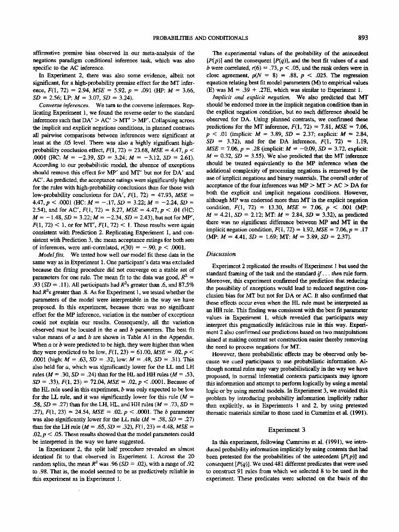
Table 4
Mean Acceptance Ratings and Standard Deviations for the Converse Inferences With Explicit and Implicit Negations for Each Rule in Experiment 2 (N = 25)
Explicit Implicit
MP' DA' AC' MT' MP' DA' AC' MT'
Rule M SD M SD M SD M SD M SD M SD M SD M SD
LL -4.16 2.21 -2.60 2.12 -1.72 2.65 -4.04 2.23 -3.96 2.21 -2.16 2.53 -2.72 2.53 -3.68 2.85 LH -4.00 2.57 0.48 3.37 0.16 3.73 -3.16 3.16 -4.36 2.04 -0.16 3.20 -1.64 3.33 -3.64 2.94 IlL -3.92 2.43 -1.52 2.99 -2.28 2.35 -4.32 1.68 -4.36 1.32 -2.68 2.43 -3.04 1.93 -3.32 2.95 HI-I -4.56 1.26 -0 .36 3.17 -1.40 2.66 -4 .08 2.29 -4.16 2.21 -0 .64 3.24 -2.64 2.56 -3 .56 3.02
Total -4.16 2.16 -1.00 3.13 -1.31 2.99 -3.90 2.40 -4.21 1.96 -1.41 3.02 -2.51 2.65 -3.55 2.90
Note. Numbers in boldface indicate a high-probability conclusion. MP = modus ponens; DA = denying the antecedent; AC = affirming the consequent; MT = modus tollens; LL = low P(p), low P(q); LH = low P(p), high P(q); HL = high P(p), low P(q); HH = high P(p), high P(q). Acceptance ratings range from - 5 to 5.
PROBABILITIES AND CONDITIONALS 893
affirmative premise bias observed in our meta-analysis of the negations paradigm conditional inference task, which was also specific to the AC inference.
In Experiment 2, there was also some evidence, albeit not significant, for a high-probability premise effect for the MT infer- ence, F(1, 72) = 2.94, MSE = 5.92, p = .091 (HP: M = 3.66, SD = 2.56; LP: M = 3.07, SD = 3.24).
Converse inferences. We turn to the converse inferences. Rep- licating Experiment 1, we found the reverse order to the standard inferences such that DA' > AC' > MT' > MP'. Collapsing across the implicit and explicit negations conditions, in planned contrasts all palrwise comparisons between inferences were significant at least at the .05 level. There was also a highly significant high- probability conclusion effect, F(1, 72) = 23.68, MSE = 4.47, p < .0001 (HC: M = -2 .39, SD = 3.24; M = -3 .12, SD = 2,61). According to our probabilistic model, the absence of exceptions should remove this effect for MP' and MT' but not for DA' and AC' . As predicted, the acceptance ratings were significantly higher for the rules with high-probability conclusions than for those with low-probability conclusions for DA' , F(1, 72) = 47.93, MSE = 4.47,p < .0001 (HC: M = - .17 , SD = 3.22; M = -2 .24, SD = 2.54), and for AC' , F(1, 72) = 8.27, MSE = 4.47, p < .01 (HC: M = - 1.48, SD = 3.22; M = -2 .34 , SD = 2.43), but not for MP' , F(1, 72) < 1, or for MT' , F(1, 72) < 1. These results were again consistent with Prediction 2. Replicating Experiment 1, and con- sistent with Prediction 3, the mean acceptance ratings for both sets of inferences, were anti-correlated, r(30) = - .90 , p < .0001.
Model fits. We tested how well our model fit these data in the same way as in Experiment 1. One participant's data was excluded because the fitting procedure did not converge on a stable set of parameters for one rule. The mean fit to the data was good, R 2 = .93 (SD = . 11). All participants had R2s greater than .6, and 87.5% had R2s greater than .8. As for Experiment 1, we tested whether the parameters of the model were interpretable in the way we have proposed. In this experiment, because there was no significant effect for the MP inference, varation in the number of exceptions could not explain our results. Consequently, all the variation observed must be located in the a and b parameters. The best fit value means of a and b are shown in Table A1 in the Appendix. When a or b were predicted to be high, they were higher than when they were predicted to be low, F(1, 23) = 61.00, MSE = .02, p < .0001 (high: M = .63, SD = .32; low: M = .48, SD = .31). This also held for a, which was significantly lower for the LL and LH rules (M = .30, SD = .24) than for the HL and HH rules (M = .53, SD = .33), F(1, 23) = 72.04, MSE = .02, p < .0001. Because of the HL rule used in this experiment, b was only expected to be low for the LL rule, and it was significantly lower for this rule (M = .58, SD = .27) than for the LH, HL, and HH rules (M = .73, SD = .27), F(1, 23) = 24.54, MSE = .02, p < .0001. The b parameter was also significantly lower for the LL n~e (M = .58, SD = .27) than for the LH rule (M = .65, SD = .32), F(1, 23) = 4.48, MSE = .02, p < .05. These results showed that the model parameters could be interpreted in the way we have suggested.
In Experiment 2, the split half procedure revealed an almost identical fit to that observed in Experiment 1. Across the 20 random splits, the mean R 2 was .96 (SD = .02), with a range of .92 to .98. That is, the model seemed to be as predictively reliable in this experiment as in Experiment 1.
The experimental values of the probability of the antecedent [P(p)] and the consequent [P(q)], and the best fit values of a and b were correlated, r(6) = .73, p < .05, and the rank orders were in close agreement, o(N = 8) = .88, p < .025. The regression equation relating best fit model parameters (M) to empirical values (IS) was M = .39 + .27E, which was similar to Experiment 1.
Implicit and explicit negation. We also predicted that MT should be endorsed more in the implicit negation condition than in the explicit negation condition, but no such difference should be observed for DA. Using planned contrasts, we confLrmed these predictions for the MT inference, F(1, 72) = 7.81, MSE --- 7.06, p < .01 (implicit: M = 3.89, SD = 2.37; explicit: M = 2.84, SD = 3.32), and for the DA inference, F(1, 72) -- 1.19, MSE = 7.06, p = .28 (implicit: M = -0 .09, SD = 3.72, explicit: M = 0.32, SD = 3.55). We also predicted that the MT inference should be treated equivalently to the MP inference when the additional complexity of processing negations is removed by the use of implicit negations and binary materials. The overall order of acceptance of the four inferences was MP > MT > AC > D A for both the explicit and implicit negations conditions. However, although MP was endorsed more than MT in the explicit negation condition, F(1, 72) = 13.30, MSE = 7.06, p < .001 (MP: M = 4.21, SD = 2.12; MT: M = 2.84, SD = 3.32), as predicted there was no significant difference between MP and MT in the implicit negation condition, F(1, 72) = 1.92, MSE = 7.06, p = .17 (MP: M = 4.41, SD = 1.69; MT: M = 3.89, SD = 2.37).
Discuss ion
Experiment 2 replicated the results of Experiment 1 but used the standard framing of the task and the s tandard / f . . , then rule form. Moreover, this experiment confirmed the prediction that reducing the possibility of exceptions would lead to reduced negative con- clusion bias for MT but not for DA or AC. It also confirmed that these effects occur even when the HL rule must be interpreted as an HH rule. This finding was consistent with the best fit parameter values in Experiment 1, which revealed that participants may interpret this pragmatically infelicitous rule in this way. Experi- ment 2 also confm-ned our predictions based on two manipulations aimed at making contrast set construction easier thereby removing the need to process negations for MT.
However, these probabilistic effects may be observed only be- cause we cued participants to use probabilistic information. Al- though normal rules may vary probabilistically in the way we have proposed, in normal inferential contexts participants may ignore this information and attempt to perform logically by using a mental logic or by using mental models. In Experiment 3, we avoided this problem by introducing probability information implicitly rather than explicitly, as in Experiments 1 and 2, by using pretested thematic materials similar to those used in Cummins et al. (1991).
Exper imen t 3
In this experiment, following Cummins et al. (1991), we intro- duced probability information implicitly by using contents that had been pretested for the probabilities of the antecedent [P(p)] and consequent [P(q)]. We used 481 different predicates that were used to construct 91 rules from which we selected 8 to be used in the experiment. These predicates were selected on the basis of the
894 OAKSFORD, CHATER, AND LARKIN
probabilities and have also been used by Oaksford et al. (1999) in Wason ' s selection task. The specific criteria used in the selection process are irrelevant because in this experiment we also included a probability rating task (PRT) to check that the probabilities conform to the relevant h igh- low patterns. The PRT was con- ducted after the main experiment to avoid cuing participants to the relevance of probabilistic information.
Polarity biases have primarily been observed with abstract ma- terial. This is why in Experiments 1 and 2 we concentrated on such materials, showing that an appropriate manipulation of probabili- ties produced related effects. According to Oaksford and Sten- n ing ' s (1992) account, the identification of contrast sets is one important function of negations that had been ignored in the reasoning literature. However, negations have many other impor- tant functions in normal discourse (see, e.g., Horn, 1989), some of which have also been appealed to in the explanation of the effects of negation in reasoning experiments (Evans, 1998). The introduc- tion of contentful material in this experiment could therefore introduce effects that may override the role of negations in iden- tifying contrast sets for the DA and MT inference. Indeed Evans has argued that polarity biases are related to matching biases that are not typically seen when contentful materials are used in rea- soning tasks. Consequently, the use of such material may make it more difficult to observe a high-probability conclusion effect. On the other hand, observation of such effects by using contentful materials would act as strong confirmation that identification of contrast sets does occur when interpreting negated claims as Oaks- ford and Stenning (1992) have argued.
Method
Participants. Twenty undergraduate psychology students from the University of Warwick took part in this experiment. Each participant was paid £4.00 ($6.50) per hour to participate. None of the participants had any prior knowledge of the conditional inference task.
Design. The experiment was a 4 × 2 x 2 × 2 Inference (MP vs. DA vs. AC vs. MT) x Conclusion (standard vs. converse) X P(p) × P(q) completely within-subject design. All participants received the probability rating task after the conditional inference task because we did not want to explicitly cue participants to attend to probability information.
Materials. The eight rules used in this experiment were as follows (from Oaksford et al., 1999, Experiment 1); two rules were used in each condition.
1. If a game is played on a rink then it is bowling. (LL) 2. If a person is a politician then they are privately educated. (LL) 3. If a drink is whisky then it is drunk from a cup. (LH) 4. If an animal is a chipmunk then it has fur. (LH) 5. If an item of food is savory then it is mousse. (HL) 6. If a vegetable is eaten cooked then it is a parsnip. (HL) 7. If a flower is under 1 foot tall then it is domestic. (HH) 8. If an item of furniture is heavy then it is big. (HH)
The materials consisted of a 65-page booklet. The fwst page of each booklet was an instruction page. Each of the following pages contained one of the 64 possible conditional inference problems. For each participant, these problems appeared in different random orders.
Procedure. Participants were tested individually. The booklet was placed face down on a desk in an experimental cubicle. Participants were sat at the desk and told not to turn over the booklet until they were instructed. On turning over the booklet, the first page revealed the follow- ing instructions:
Your task is to solve the following problems on these pages. There are 64 problems and each one is made up of a rule and a fact, followed
by a conclusion. You must determine whether the conclusion can be drawn from the rule and the fact.
Participants had to rate the acceptability of the conclusion by using a rating scale, which was also used in Experiment 2 (see also Cummins et al., 1991). On the instruction page, an example was presented with materials not used in the experiments:
For example:
If the car is a Mercedes then it is black.
This car is not black.
Therefore this car is not a Mereedes.
Given this rule and this fact, place a mark on the scale below that best reflects your evaluation of the conclusion.
Participants were then presented with the same rating scale as that used in Experiment 2. The instructions then proceeded as follows:
If you are sure that you can make this conclusion given the rule and the fact above then you would tick the scale as shown.
Please answer the questions in the order that they appear and do not go back and change your answer once you have turned over the page. Thank you.
After completing the conditional inference task, participants were given the PRT as used by Oaksford et al. (1999). For each of the eight rules, the PRT consisted of the following three questions, which we illustrate by using one of the LL rules as an example:
(Question la) Of every 100 people, bow many would you expect to be politicians?
(Question lb) Of every 100 people, how many would you expect to be privately educated?
Please estimate on a scale from 0% (must be false)-100% (must be true) the likelihood that the following statement is true:
(Question lc) If a person is a politician then they are privately educated.
Although participants were asked about the likelihood of the truth or falsity of the rules, this information failed to reveal any interesting effects. Therefore, we do not report the results here. When all participants had finished the booklet, they were thanked for their participation and were fully debriefed concerning the purpose of the experiment.
Results
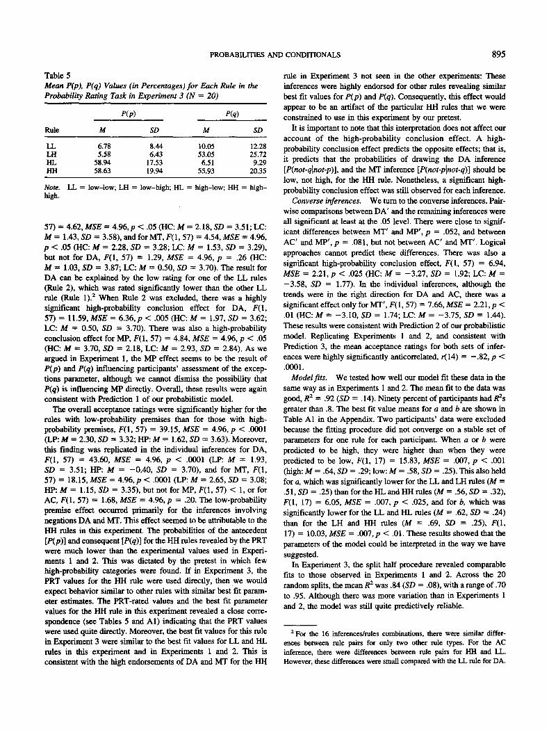
Probability rating task. The results of the PRT (see Table 5) reflected the pretest classification of the rules: When the proba- bility of the antecedent [P(p)] or consequent [P(q)] was predicted to be low, these values were well below .5 (range: .0558-.1005); when they were predicted to be high, they were all above .5 (range: .5305-.5894). All differences between high and low values of P(p) and P(q) were highly significant.
Conclusion and premise effects. The mean acceptance ratings are shown in Table 6. We analyzed these data in the same way as in Experiments 1 and 2. For the standard inferences, the accep- tance ratings were significantly higher for the inferences with high-probability conclusions than for those with low-probability conclusions, F(1, 57) = 15.88, MSE = 4.96, p < .0005 (HC: M = 2.30, SD = 3.39; LC: M = 1.59, SD = 3.46). Moreover, this finding was replicated in the individual inferences for AC, F(1,
PROBABILITIES AND CONDITIONALS 895
Table 5 Mean P(p), P(q) Values (in Percentages) for Each Rule in the Probability Rating Task in Experiment 3 (N = 20)
P(p) P(q)
Rule M SD M SD
LL 6.78 8.44 10.05 12.28 /.2-I 5.58 6.43 53.05 25.72 HL 58.94 17.53 6.51 9.29 HH 58.63 19.94 55.93 20.35
Note. I2, = low-low; LH = low-high; HL = high-low; HH = high- high.
57) = 4.62, MSE = 4.96,p < .05 (HC: M = 2.18, SD = 3.51; LC: M = 1.43, SD = 3.58), and for MT, F(1, 57) = 4.54, MSE = 4.96, p < .05 (HC: M = 2.28, SD = 3.28; LC: M = 1.53, SD = 3.29), but not for DA, F(1, 57) = 1.29, MSE = 4.96, p = .26 (HC: M = 1.03, SD = 3.87; LC: M = 0.50, SD = 3.70). The result for DA can be explained by the low rating for one of the LL rules (Rule 2), which was rated significantly lower than the other LL rule (Rule 1). 2 When Rule 2 was excluded, there was a highly significant high-probability conclusion effect for DA, F(1, 57) = 11.59, MSE = 6.36, p < .005 (HC: M = 1.97, SD = 3.62; LC: M = 0.50, SD = 3.70). There was also a high-probability conclusion effect for MP, F(1, 57) = 4.84, MSE = 4.96, p < .05 (HC: M = 3.70, SD = 2.18, LC: M = 2.93, SD = 2.84). As we argued in Experiment 1, the MP effect seems to be the result of P(p) and P(q) influencing participants' assessment of the excep- tions parameter, although we cannot dismiss the possibility that P(q) is influencing MP directly. Overall, these results were again consistent with Prediction 1 of our probabilistic model.
The overall acceptance ratings were significantly higher for the rules with low-probability premises than for those with high- probability premises, F(1, 57) = 39.15, MSE = 4.96, p < .0001 (LP: M = 2.30, SD = 3.32; HP: M = 1.62, SD = 3.63). Moreover, this finding was replicated in the individual inferences for DA, F(1, 57) = 43.60, MSE = 4.96, p < .0001 (LP: M = 1.93, SD = 3.51; HP: M = -0 .40 , SD = 3.70), and for MT, F(1, 57) = 18.15, MSE = 4.96,p < .0001 (LP: M = 2.65, SD = 3.08; liP: M = 1.15, SD = 3.35), but not for MP, F(1, 57) < 1, or for AC, F(1, 57) = 1.68, MSE = 4.96, p = .20. The low-probability premise effect occurred primarily for the inferences involving negations DA and MT. This effect seemed to be attributable to the HI-I rules in this experiment. The probabilities of the antecedent [P(p)] and consequent [P(q)] for the HH rules revealed by the PRT were much lower than the experimental values used in Experi- ments 1 and 2. This was dictated by the pretest in which few high-probability categories were found. If in Experiment 3, the PRT values for the HH rule were used directly, then we would expect behavior similar to other rules with similar best fit param- eter estimates. The PRT-rated values and the best fit parameter values for the HH rule in this experiment revealed a close corre- spondence (see Tables 5 and A1) indicating that the PRT values were used quite directly. Moreover, the best fit values for this rule in Experiment 3 were similar to the best fit values for LL and HL rules in this experiment and in Experiments 1 and 2. This is consistent with the high endorsements of DA and MT for the I-IH
rule in Experiment 3 not seen in the other experiments: These inferences were highly endorsed for other rules revealing similar best fit values for P(p) and P(q). Consequently, this effect would appear to be an artifact of the particular HH rules that we were constrained to use in this experiment by our pretest.
It is important to note that this interpretation does not affect our account of the high-probability conclusion effect. A high- probability conclusion effect predicts the opposite effects; that is, it predicts that the probabilities of drawing the DA inference [P(not-qlnot-p)], and the MT inference [P(not-plnot-q) ] should be low, not high, for the HH rule. Nonetheless, a significant high- probability conclusion effect was still observed for each inference.
Converse inferences. We turn to the converse inferences. Pair- wise comparisons between DA' and the remaining inferences were all significant at least at the .05 level. There were close to signif- icant differences between MT' and MP', p = .052, and between AC' and MP', p = .081, but not between AC' and MT' . Logical approaches cannot predict these differences. There was also a significant high-probability conclusion effect, F(1, 57) = 6.94, MSE = 2.21, p < .025 (HC: M = -3 .27, SD = 1.92; LC: M = -3 .58, SD = 1.77). In the individual inferences, although the trends were in the right direction for DA and AC, there was a significant effect only for MT' , F(1, 57) = 7.66, MSE = 2.21, p < .01 (HC: M = -3 .10 , SD = 1.74; LC: M = -3 .75, SD = 1.44). These results were consistent with Prediction 2 of our probabilistic model. Replicating Experiments 1 and 2, and consistent with Prediction 3, the mean acceptance ratings for both sets of infer- ences were highly significantly anticorrelated, r(14) = - .82 , p < .0001.
Modelfits. We tested how well our model fit these data in the same way as in Experiments 1 and 2. The mean fit to the data was good, R 2 = .92 (SD = . 14). Ninety percent of participants had R2s greater than .8. The best fit value means for a and b are shown in Table A1 in the Appendix. Two participants' data were excluded because the fitting procedure did not converge on a stable set of parameters for one rule for each participant. When a or b were predicted to be high, they were higher than when they were predicted to be low, F(1, 17) = 15.83, MSE = .007, p < .001 (high: M = .64, SD = .29; low: M = .58, SD = .25). This also held for a, which was significantly lower for the LL and LH rules (M = .51, SD = .25) than for the HL and HH rules (M = .56, SD = .32), F(1, 17) = 6.05, MSE = .007, p < .025, and for b, which was significantly lower for the LL and HL rules (M = .62, SD = .24) than for the LH and HH rules (M = .69, SD = .25), F(1, 17) = 10.03, MSE = .007, p < .01. These results showed that the parameters of the model could be interpreted in the way we have suggested.
In Experiment 3, the split half procedure revealed comparable fits to those observed in Experiments 1 and 2. Across the 20 random splits, the mean R 2 was .84 (SD = .08), with a range of .70 to .95. Although there was more variation than in Experiments 1 and 2, the model was still quite predictively reliable.
2 For the 16 inferences/rules combinations, there were similar differ- ences between rule pairs for only two other rule types. For the AC inference, there were differences between rule pairs for HH and LL. However, these differences were small compared with the LL rule for DA.
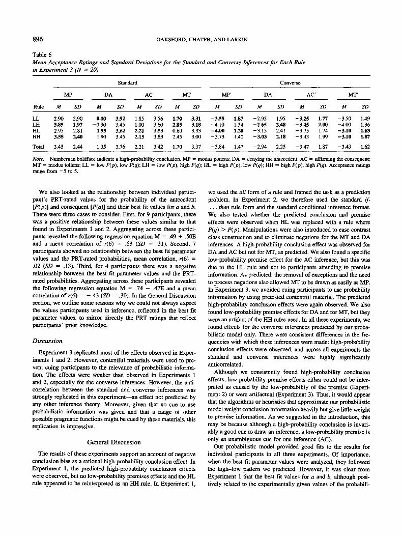
896 OAKSFORD, CHATER, AND LARKIN
Table 6 Mean Acceptance Ratings and Standard Deviations for the Standard and Converse Inferences for Each Rule in Experiment 3 (N = 20)
Standard Converse
MP DA AC MT MP' DA' AC' MT'
Rule M SD M SD M SD M SD M SD M SD M SD M SD
LL 2.90 2.90 0.10 3.92 1.85 3.56 1.70 3.31 -3.$5 1.87 -2.95 1.95 -3.25 1.77 -3.50 1.49 LH 3.85 1.97 -0.90 3.45 1.00 3.60 2.85 3.18 -4.10 1.34 -2.65 2.48 -3.45 2.00 -4.00 1.36 HL 2.95 2.81 1.95 3.62 2.21 3.53 0.60 3.33 -4.00 1.20 -3.15 2.41 -3.75 1.74 -3.10 1.63 HH 3.55 2.40 1.90 3.45 2.15 3.53 2.45 3.00 -3.73 1.40 -3.03 2.18 -3.43 1.99 -3.10 1.87
Total 3.45 2.44 1.35 3.76 2.21 3.42 1.70 3.37 -3.84 1.47 -2.94 2.25 -3.47 1.87 -3.43 1.62
Note. Numbers in boldface indicate a high-probability conclusion. MP = modus ponens; DA = denying the antecedent; AC = affirming the consequent; MT = modus tollens; LL = low P(p), low P(q); LH = low P(p), high P(q); HL = high P(p), low P(q); HH = high P(p), high P(q). Acceptance ratings range from - 5 to 5.
We also looked at the relationship between individual partici- pant's PRT-rated values for the probability of the antecedent [P(p)] and consequent [P(q)] and their best fit values for a and b. There were three cases to consider. First, for 9 participants, there was a positive relationship between these values similar to that found in Experiments 1 and 2. Aggregating across these partici- pants revealed the following regression equation M = .49 + .50E and a mean correlation of r(6) = .63 (SD = .31). Second, 7 participants showed no relationship between the best fit parameter values and the PRT-rated probabilities, mean correlation, r(6) = .02 (SD -- .13). Third, for 4 participants there was a negative relationship between the best fit parameter values and the PRT- rated probabilities. Aggregating across these participants revealed the following regression equation M = .74 - .47E and a mean correlation of r(6) = - . 4 3 (SD = .30). In the General Discussion section, we outline some reasons why we could not always expect the values participants used in inference, reflected in the best fit parameter values, to mirror directly the PRT ratings that reflect participants' prior knowledge.
Discuss ion
Experiment 3 replicated most of the effects observed in Exper- iments 1 and 2. However, contentful materials were used to pre- vent cuing participants to the relevance of probabilistic informa- tion. The effects were weaker than observed in Experiments 1 and 2, especially for the converse inferences. However, the anti- correlation between the standard and converse inferences was strongly replicated in this experiment--an effect not predicted by any other inference theory. Moreover, given that no cue to use probabilistic information was given and that a range of other possible pragmatic functions might be cued by these materials, this replication is impressive.
Genera l Discuss ion
The results of these experiments support an account of negative conclusion bias as a rational high-probability conclusion effect. In Experiment 1, the predicted high-probability conclusion effects were observed, but no low-probability premises effects and the HL rule appeared to be reinterpreted as an HH rule. In Experiment 1,
we used the all form of a rule and framed the task as a prediction problem. In Experiment 2, we therefore used the standard if- . . . then rule form and the standard conditional inference format.
We also tested whether the predicted conclusion and premise effects were observed when HL was replaced with a rule where P(q) > P(p). Manipulations were also introduced to ease contrast class construction and to eliminate negations for the MT and DA inferences. A high-probability conclusion effect was observed for DA and AC but not for MT, as predicted. We also found a specific low-probability premise effect for the AC inference, but this was due to the HL rule and not to participants attending to premise information. As predicted, the removal of exceptions and the need to process negations also allowed MT to be drawn as easily as MP. In Experiment 3, we avoided cuing participants to use probability information by using pretested contentful material. The predicted high-probability conclusion effects were again observed. We also found low-probability premise effects for DA and for MT, but they were an artifact of the HH rules used. In all these experiments, we found effects for the converse inferences predicted by our proba- bilistic model only. There were consistent differences in the fre- quencies with which these inferences were made: high-probability conclusion effects were observed, and across all experiments the standard and converse inferences were highly significantly anticorrelated.
Although we consistently found high-probability conclusion effects, low-probability premise effects either could not be inter- preted as caused by the low-probability of the premise (Experi- ment 2) or were artifactual (Experiment 3). Thus, it would appear that the algorithms or heuristics that approximate our probabilistic model weight conclusion information heavily but give little weight to premise information. As we suggested in the introduction, this may be because although a high-probability conclusion is invari- ably a good cue to draw an inference, a low-probability premise is only an unambiguous cue for one inference (AC).
Our probabilistic model provided good fits to the results for individual participants in all three experiments. Of importance, when the best fit parameter values were analyzed, they followed the high-low pattern we predicted. However, it was clear from Experiment 1 that the best fit values for a and b, although posi- tively related to the experimentally given values of the probabili-
PROBABILITIES AND CONDITIONALS 897
ties of the antecedent [P(p)] and the consequent [P(q)], were quite dissimilar. This was also found in Experiment 3 in which partic- ipants were asked to provide estimates of these probabilities in the PRT. We suspect that the reason for this apparent mismatch is that the experimentally given values (Experiments 1 and 2) or prior knowledge (Experiment 3) of these probabilities must interact with further assumptions that are specific to when inferences need to be made.
For example, suppose someone is in his or her kitchen at home. It is unlikely that within this context this person's knowledge that donkeys are stubborn is primed ready to infer that a particular animal is stubborn given that he or she has identified it as a donkey. However, if this person were on a farm, then this knowl- edge may well be primed ready to make this inference if required. Being "primed" here means something to the effect that there is a highly probability of encountering a donkey (i.e., this knowledge is primed in contexts in which you are likely to encounter don- keys). That is, inferences are only relevant when the properties or events to which they apply are more likely than normal to occur. Consequently, although the base rate of donkeys may be low, in a context in which it would be appropriate to draw inferences about donkeys, P(donkey) may be considered to be much higher. In summary, there is every reason to expect divergences between individual best fit parameter values and either the experimentally given values or even participants' own assessments of the base rates of the properties or events in the rules. Although Experi- ments 1 and 2 showed that these values are related, Experiment 3 showed considerable variation in the relationship between partic- ipants' prior beliefs and the probability values used in inference. Although almost half of the participants followed a similar pattern to Experiments 1 and 2, others seemed to show no systematic relationship between their prior knowledge revealed in the PRT and their best fit parameter values. This may reflect different strategies that emerge in responding to the task demands and in dealing with unfamiliar material. The examination of different strategies for using prior knowledge in the context of an unfamiliar inferential task is an area for further research.
Evans et al. (1995) argued that their results show that negative conclusion bias is restricted to DA and MT and hence can be explained as a double negation effect; that is, to infer the conclu- sion for both inferences, participants must realize that not-not-p is equivalent to p. According to the contrast set account of negation, our probabilistic model also predicts a negative conclusion bias for AC. Therefore, Evans et al.'s experiments seem to contradict our model. However, our meta-analysis of the negations paradigm studies (see introduction) showed a significant negative conclusion bias for the AC inference, which is not consistent with the double negation hypothesis. Consequently, it would appear that Evans et al.'s findings represent the anomalous result and not our experi- ments in which we consistently found an analogous high- probability conclusion effect for AC.
Recently, Evans and Handley (1999) found that when implicit negations are used in the categorical premise (see our Experiment 2), a strong affirmative premise bias is observed but not a negative conclusion bias. Participants withheld endorsing inferences from implicitly negated categorical premises. 3 Evans (1998) has rein- terpreted this effect as continuous with matching effects in other reasoning tasks (e.g., Evans, 1972; Evans & Lynch, 1973). These results seem inconsistent with our explanation of conditional in-
ference biases. However, the contrast set account of negations may explain Evans and Handley's results.
On a probabilistic interpretation, it can be consistent to beheve that a conclusion should be drawn when a negated categorical premise is presented in explicit form and that it should not be drawn when that same premise is presented in implicit form. Consider the two contingency tables in Table 7. Table 7A repre- sents a dependency between two classes p and a (i.e., i f p, then a). The p class can be thought of as the set of ravens, and a as the set of black birds. Table 7A also represents the dependency that /f not-p, then not-a. Table 7B represents this same information but uses contrast set members to encode the negatives. The sets P = {p, q, r} and A = {a, b, c} are exhaustive. P can be thought of as the set of birds, and A as the set of colors. So now i fx is not a, then it is either b or c (e.g., if a bird is not a raven, then its either a crow or a robin). Suppose that someone were asked to assess the DA inference if p then a, not-p, therefore not-a. Whether the proba- bilities are calculated over Table 7A or Table 7B, the same answer is produced: P(not-alnot-p) = .833. Therefore, according to our model, participants should strongly endorse not-a as the conclu- sion. Suppose now that someone is asked to assess the same inference by using a contrast set member as the categorical premise; that is, if not-p then not-a, q (C not-p), therefore not-a. According to Table 7B, P(not-alq ) = .333, and therefore partici- pants should endorse not-a as the conclusion quite weakly. This example suggests that participants may be unlikely to endorse inferences with implicitly negated categorical premises. Conse- quently, the affmnative premise bias observed by Evans and Handley (1999) could be predicted from a rational probabilistic perspective, Moreover, such a bias would suppress a negative conclusion bias because each bias works against the other: they disagree on two rules for each inference (e.g., for DA they disagree on AA and NN). Evans and Handley (1999) may have found little evidence for negative conclusion bias because it has been overrid- den by the effects of implicit negations.
Probabilistic effects such as those we present here seem incon- sistent with either mental logic accounts (e.g., Rips, 1994) in which people are held to draw inferences by using syntactic rules as in formal logic or mental models theory (e.g., Johnson-Laird & Byrne, 1991), in which people are held to reason by manipulating arbitrary mental tokens representing the meanings of sentences. First, there are no current proposals in the mental logic approach to account for probabilistic effects. However, the mental logician may argue that they do not need to account for such effects because the tasks we have used do not solely engage logical reasoning. This argument may make sense for Experiments 1 and 2, in which probabilistic information was explicitly introduced but cannot apply to Experiment 3, in which this information was left implicit. Mental models theorists on the other hand have directly confronted the issue of probabilistic effects. Johnson-Laird et al. (1999) have argued that in realistic settings in which prior knowledge is available, individual mental models may be anno- tated with probabilities, as proposed by Stevenson and Over (1995). Johnson-Laird et al. (1999) proposed that, perhaps elemen- tary, probabilistic calculations over these numbers can explain
3 Some caution is required in this interpretation because with implicit negations every categorical premise is now, in a sense, affirmative.

898 OAKSFORD, CHATER, AND LARKIN
Table 7 Illustrative Examples of Contingency Tables for a Conditional Rule
A B A
a no~a a b c
p .3 .1 p .3 .05 .05 not-p .1 .5 P q .1 .025 .025
r 0 .225 .225
Note. Examples use explicit negations (A) and implicit negations (B) in which, for example, not-a = {b, c}.
probabilistic effects in reasoning. However, these processes are clearly dissimilar in kind to the manipulation of mental models, and so there is no theory of these effects that intrinsically relies on the notion of a mental model.
In this article, we have argued that polarity biases in condi- tional inference can be explained within a simple rational probabilistic framework. Our experiments are consistent with the view that negative conclusion bias is really a rational high-probability conclusion effect as predicted by the contrast set account of negations (Oaksford & Chater, 1994, 1998b; Oaksford & Stenning, 1992). In the discussion, we outlined how the effects of implicit negations may also be incorporated in a probabilistic account. Together with our probabilistic accounts of the selection task (Oaksford & Chater, 1994) and syllogistic reasoning (Chater & Oaksford, 1999b), we have now offered probabilistic interpretations in the three main areas of human reasoning. It therefore seems that to explain participants' rea- soning in laboratory tasks, we must take account of the fact that everyday inferential strategies must deal with the uncertainty of the everyday world. It is these everyday uncertain reasoning strategies that people use in the laboratory and that create the semblance of biased and irrational reasoning when compared with the standard provided by formal logic.
Refe rences
Anderson, J. R. (1995). Cognitive psychology and it implications. New York: W. H. Freeman.
Apostel, L. (1972). The relation between negation in linguistics, logic and psychology. Logique et Analyse, 15, 333-401.
Chan, D., & Chua, F. (1994). Suppression of valid inferences: Syntactic views, mental models, and relative salience. Cognition, 53, 217-238.
Chater, N., & Oaksford, M. (1999a). Information gain and decision theo- retic approaches to data selection. Psychological Review, 106, 223-227.
Chater, N., & Oaksford, M. (1999b). The probability heuristics model of syllogistic reasoning. Cognitive Psychology, 38, 191-258.
Comrie, B. (1986). Conditionals: A typology. In E. C. Traugott, A. ter Meulen, J. S. ReiUy, & C. A. Ferguson (Eds.), On conditionals (pp. 77-99). Cambridge, England: Cambridge University Press.
Cummins, D. D., Lubart, T., Alksnis, O., & Rist, R. (1991). Conditional reasoning and causation. Memory & Cognition, 19, 274-282.
Evans, J. St.B.T. (1972). Interpretation and "matching bias" in a reasoning task. Quarterly Journal of Experimental Psychology, 24, 193-199.
Evans, J. St.B.T. (1977). Linguistic factors in reasoning. Quarterly Jour- nal of Experimental Psychology, 29, 297-306.
Evans, J. St.B.T. (1983). Linguistic determinants of bias in conditional
reasoning. Quarterly Journal of Experimental Psychology, 35,4, 635- 644.
Evans, J. St.B.T. (1993). The mental model theory of conditional reason- ing: Critical appraisal and revision. Cognition, 48, 1-20.
Evans, J. St.B.T. (1998). Matching bias in conditional reasoning: Do we understand it after 25 years? Thinking and Reasoning, 4, 45-82.
Evans, J. St.B.T., Clibbens, J., & Rood, B. (1995). Bias in conditional inference: Implications for mental models and mental logic. Quarterly Journal of Experimental Psychology, 48,4, 644-670.
Evans, J. St.B.T., & Handley, S. J. (1999). The role of negation in conditional inference. Quarterly Journal of Experimental Psychol- ogy, 52, 739-770.
Evans, J. St.B.T., & Lynch, J. S. (1973). Matching bias in the selection task. British Journal of Psychology, 64, 391-397.
Evans, J. St.B.T., Newstead, S. E., & Byrne, R. M. J. (1993). Human reasoning. HiUsdale, NJ: Erlbaum.
George, C. (1997). Reasoning from uncertain premises. Thinking and Reasoning, 3, 161-190.
Gigerenzer, G., & Hoffrage, U. (1995). How to improve Bayesian reason- ing without instruction: Frequency formats. Psychological Review, 102, 684-704.
Horn, L. R. (1989). A natural history of negation. Chicago: Chicago University Press.
Johnson-Laird, P. N., & Byrne, R. M. J. (1991). Deduction. HiUsdale, NJ: Erlbaum.
Johnson-Laird, P. N., Legrenzi, P., Girotto, V., Legrenzi, M. S., & Caverni, J. (1999). Naive probability: A mental model theory of extensional reasoning. Psychological Review, 106, 62-88.
Kern, L. H., Mirels, H. L., & Hinshaw, V. G. (1983). Scientists' under- standing of propositional logic: An experimental investigation. Social Studies of Science, 13, 131-146.
Kirby, K. N. (1994). Probabilities and utilities of fictional outcomes in Wason's four card selection task. Cognition, 51, 1-28.
Liu, I., Lo, K., & Wu, J. (1996). A probabilistic interpretation of "If-then." Quarterly Journal of Experimental Psychology, 49A, 828-844.
Marcus, S. L., & Rips, L. J. (1979). Conditional reasoning. Journal of Verbal Learning and Verbal Behavior, 18, 199-223.
Markovits, H. (1988). Conditional reasoning, representation, empirical evidence on a concrete task. Quarterly Journal of Experimental Psy- chology, 40A, 483-495.
Marr, D. (1982). Vision. San Francisco: Freeman. Oaksford, M. (1998). Task demands and revising probabilities in the
selection task. Thinking and Reasoning, 4, 179-186. Oaksford, M., &Chater, N. (1994). A rational analysis of the selection task
as optimal data selection. Psychological Review, 101, 608-631. Oaksford, M., & Chater, N. (1996). Rational explanation of the selection
task. Psychological Review, 103, 381-391. Oaksford, M., & Chater, N. (1998a). A revised rational analysis of the
selection task: Exceptions and sequential sampling. In M. Oaksford & N. Chater (Eds.), Rational models of cognition (pp. 372-398). Oxford, England: Oxford University Press.
Oaksford, M., &Chater, N. (1998b). Rationality in an uncertain worM: Essays on the cognitive science of human reasoning. Hove, England: Psychology Press.
Oaksford, M., Chater, N., & Grainger, B. (1999). Probabilistic effects in data selection. Thinking and Reasoning, 5, 193-243.
Oaksford, M., & Stenning, K. (1992). Reasoning with conditionals con- taining negated constituents. Journal of Experimental Psychology: Learning, Memory, and Cognition, 18, 835-854.
Polk, T. A., & Newell, A. (1995). Deduction as verbal reasoning. Psycho- logical Review, 102, 533-566.
Pollard, P., & Evans, J. S. T. (1980). The influence of logic on conditional reasoning performance. Quarterly Journal of Experimental Psychol- ogy, 32, 605-624.
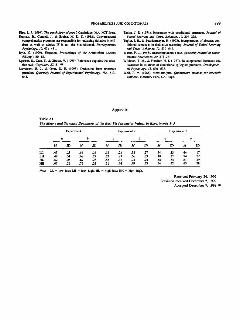
PROBABILITIES AND CONDITIONALS 899
Rips, L. J. (1994). The psychology ofproof. Cambridge, MA: MIT Press. Rumain, B., Connell, J., Rr Braine, M. D. S. (1983). Conversational
comprehension processes are responsible for reasoning fallacies in chil- dren as well as adults: IF is not the biconditional. Developmental Psycho/ogy, 19, 471-481.
Ryle, G. (1929). Negation. Proceedings of the Aristotelian Society, 9(Supp.), 80 -86 .
Sperber, D., Cara, F., & Girotto, V. (1995). Relevance explains the selec- tion task. Cognition, 57, 31-95.
Stevenson, R. J., & Over, D. E. (1995). Deduction from uncertain premises. Quarterly Journal of Experimental Psychology, 48A, 613- 643.
Taplin, J. E. (1971). Reasoning with conditional sentences. Journal of Verbal Learning and Verbal Behavior, 10, 219-225.
Taplin, J. E., & Staudenmayer, H. (1973). Interpretation of abstract con- ditionai sentences in deductive reasoning. Journal of Verbal Learning and Verbal Behavior, 12, 530-542.
Wason, P. C. (1968). Reasoning about a rule. Quarterly Journal of Exper- imental Psychology, 20, 273-281.
Wildman, T. M., & Fletcher, H. J. (1977). Developmental increases and decreases in solutions of conditional syllogism problems. Developmen- tal Psychology, 13, 630-636.
Wolf, F. M. (1986). Meta-analysis: Quantitative method.~ for research synthesis. Newbury Park, CA: Sage.
Appendix
Table A1 The Means and Standard Deviations of the Best Fit Parameter Values in Experiments 1-3
Experiment 1 Experiment 2 Experiment 3
a b a b a b
M SD M SD M SD M SD M SD M SD
LL .43 .28 .56 .27 .32 .22 .58 .27 .54 .23 .64 .17 LH .49 .31 .68 .29 .27 .27 .66 .33 .48 .27 .74 .22 I'lL .52 .25 .62 .25 .55 .33 .74 .24 .58 .34 .61 .29 HH .67 .26 .75 .24 .51 .34 .79 .23 .54 .32 .63 .28
Note. LL -- low-low; LH -- low-high; HL = high-low; HH = high-high.
Received February 24, 1999 Revision received December 2, 1999
Accepted December 7, 1999 •