Problem Set 4 for MAE280A Linear Systems Theory, Fall 2017:due Tuesday November 28, 2017, in class

Problem 1 – Controllability and reachability

Consider the RC-circuit depicted in class on Slide 3 of the Controllability lecture sequence. RC-circuit example

state is the set of capacitor voltages ! state equation

Transition function/matrix exponential

!

!

Solution

!

If R1C1=R2C2 and x(0)=0 then the state is always a scalar multiple of So Likewise, to transfer x0 to the origin !So as well

When R1C1≠R2C2 we will find that

x(t) =

v1(t)v2(t)

�

e

24

�1R1C1

0

0 �1R2C2

35t

=

"e

�1R1C1

t 0

0 e�1

R2C2t

#

Example

!3

+_

R1 R2

C1 C2+ +- -v1 v2u

11

�

R[t0, t1] =

⇢�

11

�: � � R

�

C[t0, t1] =

⇢�

11

�: � � R

�0 = e

�1R1C1

tx(0) + �

11

�

R[t0, t1] = C[t0, t1] = R2

x(t) =

�1R1C1

0

0 �1R2C2

�x +

1R1C1

1R2C2

�u

x(t) =

"e

�1R1C1

tx1(0)

e�1

R2C2tx2(0)

#+

Z t

0

"1

R1C1e

�1R1C1

(t�⌧)

1R2C2

e�1

R2C2(t�⌧)

#u(⌧) d⌧

The state-space system is described by

xt =

[−1/R1C1 0

0 −1/R2C2

]xt +

[1/R1C2

1/R2C2

]ut.

For our particular choice of resistors and capacitors, we rewrite the state equations in units of seconds×10−4 as

xt =

[−1 00 −2

]xt +

[12

]ut.

Find a control signal, ut, for t ∈ [0, 1] that transfers the state from

x0 =

[11

], to x1 =

[57

].

[Bonus] Find the minimum-energy control signal. Compute the energy.

Hint for both parts: look at the Slides 4 and 5 of the Controllability notes.

Solution:

The solution for LTI system is

x(t) = eA(t−t0)x(t0) +

∫ t

t0

eA(t−τ)Bu(τ)dτ,

we substitute the matrix A,B and state of the systems at two different time.

x(1) =

[57

]= eA(1−0)

[11

]+

∫ 1

0eA(1−τ)

[12

]u(τ)dτ,

since matrix A is diagonal then we have

eAt =

[e−t 00 e−2t

]and also, eA(1−τ) =

[e−1(1−τ) 0

0 e−2(1−τ)

]=

[e(τ−1) 0

0 e2(τ−1)

].

Now let us check if the system is reachable,

C =[B AB

]=

[1 −12 −4

]

rank of matrix C is 2, hence the system is reachable.

Use the solution equation above and see that we want to drive the zero-state solution

xzs(t) =

∫ 1

0eA(1−τ)

[12

]u(τ)dτ,

from xzs(0) =

[00

]to xzs(1) =

[57

]− eA×1

[11

].

Now we are allow to apply results from Lecture 4,

WR(0, 1) =

∫ 1

0eA(1−τ)

[12

] [1 2

]eA(1−τ)

Tdτ =

∫ 1

0

[e(τ−1) 0

0 e2(τ−1)

] [12

] [1 2

] [e(τ−1) 0

0 e2(τ−1)

]dτ

WR(0, 1) =

∫ 1

0

[e(τ−1)

2e2(τ−1)

] [e(τ−1) 2e2(τ−1)

]dτ =

∫ 1

0

[e2(τ−1) 2e3(τ−1)

2e3(τ−1) 4e4(τ−1)

]dτ

WR(0, 1) =

[(1− e−2)/2 2(1− e−3)/32(1− e−3)/3 (1− e−4)

]

According to Lecture 4, we need to find η such that

xzs(1) =

[57

]− eA×1

[11

]= WR(0, 1)η ∈ ImWR(0, 1),

then, for t ∈ [0, 1] control function,

U(t) = B(t)T eA(1−t)Tη =

[1 2

] [et−1 0

0 e2(t−1)

]η.

The minimum energy is

E =

∫ 1

0||U(τ)||2dτ = xzs(1)TWR(0, 1)−1xzs(1).

Problem 2 – Observers with real aeroengine data

The file signal.dat contains data from an experiment at United Technologies Research Center examiningcombustion instabilities in a jet engine single-nozzle rig. The combustion instability manifests as an audiblesingle tone, sometimes called hooting or howling coming from the engine. The instability is undesirable andcauses NOx pollution. The data file contains three columns of numbers: the current time, the pressure signalinside the combustor, and the heat release rate measured with a thermal sensor. You task is to build an observerto estimate the time delay between the peaks in the pressure signal and the peaks in the heat release rate signal.You need to build an observer to do this.

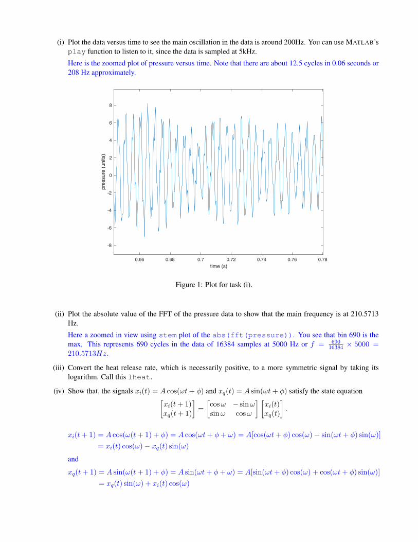
(i) Plot the data versus time to see the main oscillation in the data is around 200Hz. You can use MATLAB’splay function to listen to it, since the data is sampled at 5kHz.

Here is the zoomed plot of pressure versus time. Note that there are about 12.5 cycles in 0.06 seconds or208 Hz approximately.

0.66 0.68 0.7 0.72 0.74 0.76 0.78time (s)

-8

-6

-4

-2

0

2

4

6

8pr

essu

re (u

nits

)

Figure 1: Plot for task (i).

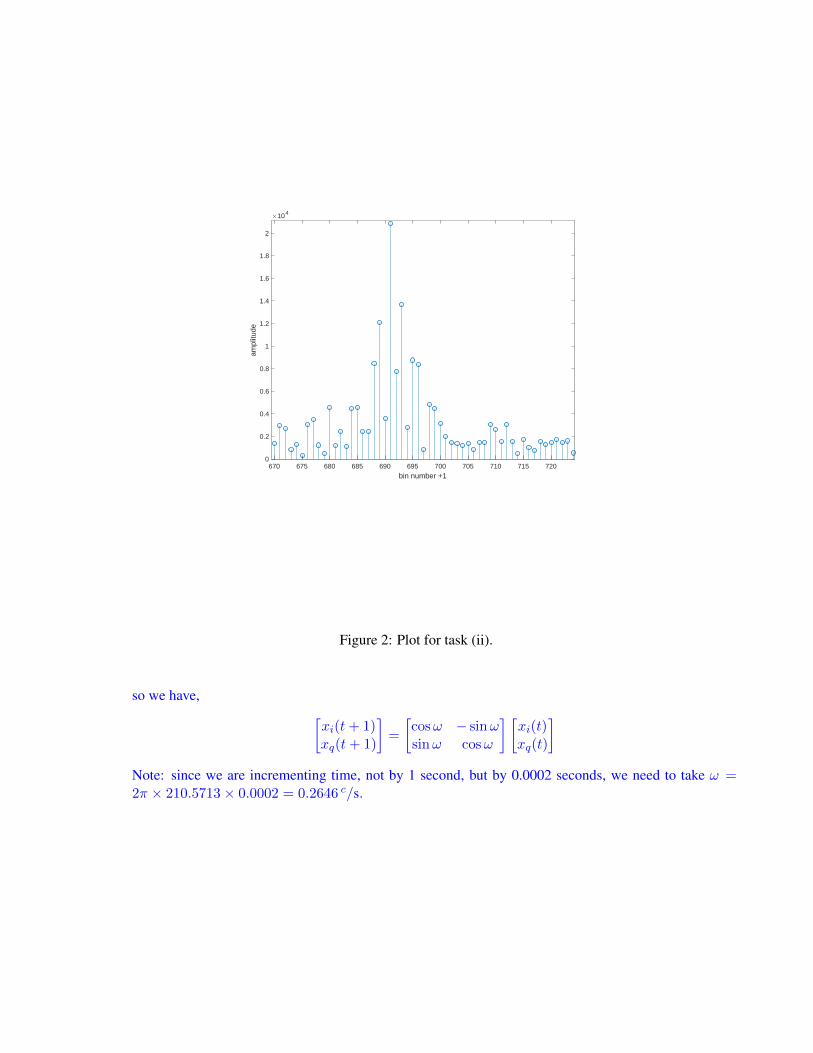
(ii) Plot the absolute value of the FFT of the pressure data to show that the main frequency is at 210.5713Hz.

Here a zoomed in view using stem plot of the abs(fft(pressure)). You see that bin 690 is themax. This represents 690 cycles in the data of 16384 samples at 5000 Hz or f = 690

16384 × 5000 =210.5713Hz.

(iii) Convert the heat release rate, which is necessarily positive, to a more symmetric signal by taking itslogarithm. Call this lheat.

(iv) Show that, the signals xi(t) = A cos(ωt+ φ) and xq(t) = A sin(ωt+ φ) satisfy the state equation[xi(t+ 1)xq(t+ 1)

]=

[cosω − sinωsinω cosω

] [xi(t)xq(t)

].

xi(t+ 1) = A cos(ω(t+ 1) + φ) = A cos(ωt+ φ+ ω) = A[cos(ωt+ φ) cos(ω)− sin(ωt+ φ) sin(ω)]

= xi(t) cos(ω)− xq(t) sin(ω)

and

xq(t+ 1) = A sin(ω(t+ 1) + φ) = A sin(ωt+ φ+ ω) = A[sin(ωt+ φ) cos(ω) + cos(ωt+ φ) sin(ω)]

= xq(t) sin(ω) + xi(t) cos(ω)

0

0.2

0.4

0.6

0.8

1

1.2

1.4

1.6

1.8

2

ampl

itude

104

670 675 680 685 690 695 700 705 710 715 720

bin number +1

Figure 2: Plot for task (ii).

so we have,[xi(t+ 1)xq(t+ 1)

]=

[cosω − sinωsinω cosω

] [xi(t)xq(t)

]

Note: since we are incrementing time, not by 1 second, but by 0.0002 seconds, we need to take ω =2π × 210.5713× 0.0002 = 0.2646 c/s.

(v) Accordingly, argue for the following being a state-space realization for pressure and for lheat.

xpi (t+ 1)xpq(t+ 1)xhi (t+ 1)xhq (t+ 1)

=

cosω − sinω 0 0sinω cosω 0 0

0 0 cosω − sinω0 0 sinω cosω

xpi (t)xpq(t)xhi (t)xhq (t)

,

[pressure(t)lheat(t)

]=

[1 0 0 00 0 1 0

]

xpi (t)xpq(t)xhi (t)xhq (t)

.

That is, this model describes pressure= A cos(ωt+φp) and lheat= B cos(ωt+φh) with the samefrequency ω but differing amplitudes A and B and differing phases φp and φh. Note that this model hasno input signal, since the audible oscillation is self-supporting.

This is fairly obvious, since both pressure and lheat are described by separate signals with the samefrequency.

(vi) If you had the full dimension 4 state x(t) available, determine an approach to compute A, B, ωt + φp

and ωt+ φh at that time from the state elements.

From part (iv) we see that

A =√

(xpi (t))2 + (xpq(t))2 and ωt+ φp = atan2(xpq(t), x

pi (t)).

and also

B =√

(xhi (t))2 + (xhq (t))2 and ωt+ φh = atan2(xhq (t), xhi (t)).

(vii) Work a bit harder and derive a formula for estimating φh − φp as a function of the state. Work evenharder still and express this phase difference at this ω as a time delay.

Start with the following trigonometric formulæ.

AB cos(φh − φp) = AB cos[(ωt+ φh)− (ωt+ φp)],

= AB cos(ωt+ φh) cos(ωt+ φp) +AB sin(ωt+ φh) sin(ωt+ φp),

= xhi (t)× xpi (t) + xhq (t)× xpq(t).AB sin(φh − φp) = AB sin[(ωt+ φh)− (ωt+ φp)],

= AB sin(ωt+ φh) cos(ωt+ φp)−AB cos(ωt+ φh) sin(ωt+ φp),

= xhq (t)× xpi (t)− xhi (t)× xpq(t).

So,

φh − φp = atan2(AB sin(φh − φp), AB cos(φh − φp)),= atan2

[xhq (t)× xpi (t)− xhi (t)× xpq(t), xhi (t)× xpi (t) + xhq (t)× xpq(t)

].

Since this is a radian phase difference of a signal at radian frequency ω radians/sec, the time difference is

τ =φh − φp

ω.

(viii) Using the value ω = 2π × 210.5713 rad/s, write this model in MATLAB. Call the matrices A and C asusual.

Do not forget to include the sampling time of Ts = 0.0002 s.

(ix) Show that the entire state is observable from the two outputs for this model.

We can check the rank of the observability matrix, which is the controllability matrix of A′ and C ′.

rank(ctrb(A’,C’))=4

(x) Select an appropriate place for observer poles and determine using place an observer output-injectiongain. Note that this is all in discrete time.

I tried two selections: 0.98 × eig(A) and 0.975 × eig(A). Both were found using commands likeL=place(A’,C’,0.98*eig(A))’.

(xi) Write the MATLAB code to do the following.

(a) Start from an initial state estimate of, say, zero and run this observer, taking the two measurements,pressure(t) and lheat(t) as inputs and yielding state estimate x(t) as its output.In general we have observer

x(t+ 1) = (A− LC)x(t) +Bu(t) + Ly(t).

In this problem we do have u(t) = 0 so

x(t+ 1) = (A− LC)x(t) + Ly(t)

Since we want all elements of the state estimate, we have

A = (A− LC), B = L, C = eye(4), D = 0

and our observer is defined as the following system,

observ=ss(A-LC, L,eye(4),zeros(4,2),1/5000)

Here are the zoomed plots of state estimates with each set of poles.

(b) Apply your formula from step ?? to compute the time delay estimate between pressure and heatrelease rate over the entire data set.

(xii) Plot your estimate over time.

Let’s take things slowly. Here are the sin term plot(time,xhq.*xpi-xhi.*xpq) and the costerm plot(time,xhi.*xpi+xhq.*xpq), where

xpi = xhat(:,1);xpq = xhat(:,2);xhi = xhat(:,3);xhq = xhat(:,4);

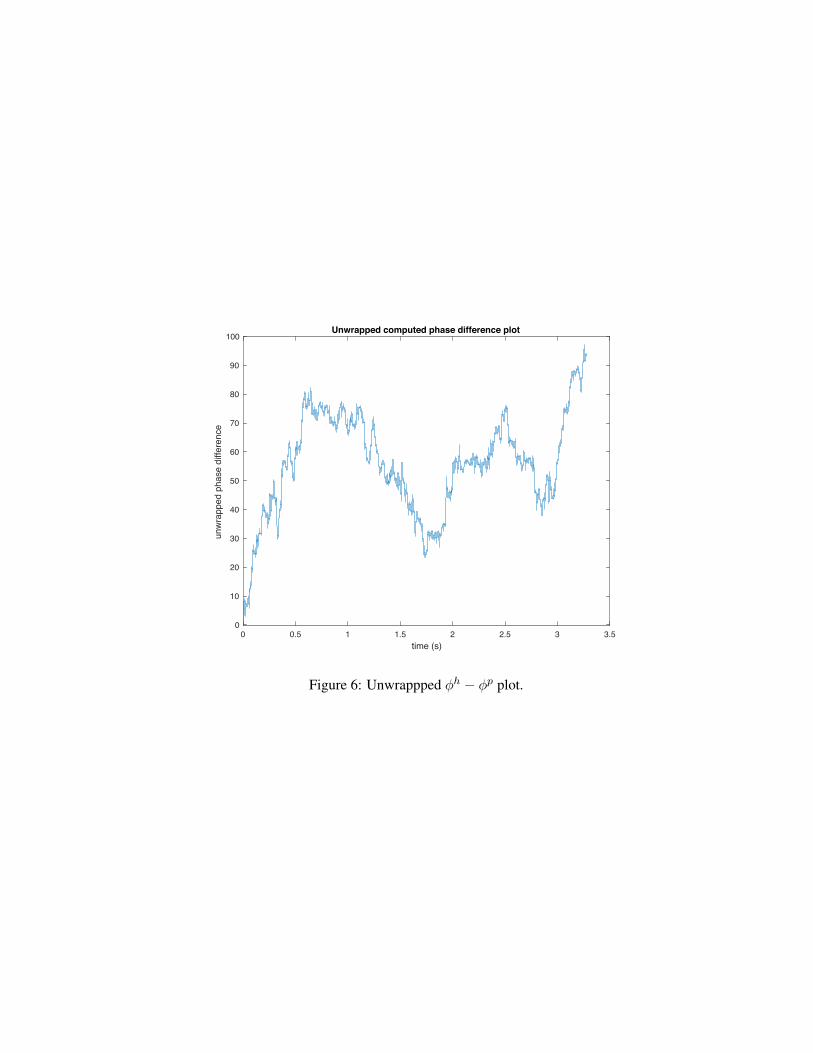
Now consider the computed phase difference: atan2(xhq.*xpi-xhi.*xpq,xhi.*xpi+xhq.*xpq).We see that the computed phase difference is jumping over 2π a lot. Let’s unwrap it. This suggests thatthe computed phase difference via atan2(.,.) is unreliable, since it is drifting over time.

Take a backward step and use the mean sin and cos terms to compute

1.03 1.04 1.05 1.06 1.07 1.08 1.09 1.1 1.11time (s)

-4

-3

-2

-1

0

1

2

3

4

5

xhat

poles 0.98*eig(A)

atan2(mean(xhq.*xpi-xhi.*xpq),mean(xhi.*xpi+xhq.*xpq)) = -0.0555.

Now add the phase difference from the differentiator, π2 , and the negatively sloped memoryless nonlin-earity, π, to get a total phase difference of 4.1273 radians or a time delay of τ = 4.1273/(ω× 0.0002) =0.0036 seconds.

Hint: I get something like delay τ=3.7 ms on average.

Welcome to the world of state estimation. The time delay is a central modeling parameter describing thepropagation time of the fuel exiting the nozzle to the flame front.

1.03 1.04 1.05 1.06 1.07 1.08 1.09time (s)

-3

-2

-1

0

1

2

3

4

xhat

poles 0.975*eig(A)

0 0.5 1 1.5 2 2.5 3 3.5time (s)

-1

0

1

ABsi

n(h -

p )

10-32 ABsin( h- p) plot

Figure 3: AB sin plot: mean -3.3054e-35.

0 0.5 1 1.5 2 2.5 3 3.5time (s)

-1.5

-1

-0.5

0

0.5

1

1.5

ABco

s(h -

p )

10-32 ABcos( h- p) plot

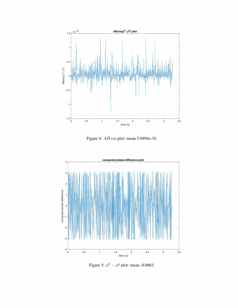
Figure 4: AB cos plot: mean 5.9494e-34.

0 0.5 1 1.5 2 2.5 3 3.5time (s)

-4

-3

-2

-1

0

1

2

3

4

com

pute

d ph

ase

diffe

renc

e

computed phase difference plot

Figure 5: φh − φp plot: mean -0.0663.

0 0.5 1 1.5 2 2.5 3 3.5time (s)

0

10

20

30

40

50

60

70

80

90

100

unw

rapp

ed p

hase

diff

eren

ce

Unwrapped computed phase difference plot

Figure 6: Unwrappped φh − φp plot.