problem set iii responsepeople.csail.mit.edu/halordain/digital image processing...christopher tsai...

Christopher Tsai April 29, 2007

EE 368 – Digital Image Processing

of 21

Problem Set III

Problem 1 – Linear Image Filtering and Sampling with the Zoneplate Image

The equation used to generate the Zoneplate pattern in ‘zoneplate.tif’ is

, ·

To determine the spatial frequency of this two-dimensional sinusoid, we first extract the phase argument:

,

By definition, the angular frequency is the rate of change in the phase along the direction of interest.

Applying the Chain Rule from multivariate calculus, we differentiate the phase:

,2

,2

In order to center our 512 512 pattern about the central pixel, we select a half-shift: 256.

Because we also seek an amplitude swing from 16 to 240 (centered on 128), we fix a constant DC term of

128. The amount of cosinusoidal oscillation in either direction is 112. Finally, in order to

ensure a full frequency sweep from 0 to π from the center, we need 2 | , and

2 , forcing us to choose 0.006136. Thus, we use parameters:

256

256

128

112

0.006136

0.006136



of 21

Displaying our artificially generated zoneplate pattern next to the actual test image zoneplate.tif, we see

The test zoneplate image looks identical to our formula-fabricated rendition for 112. Subtracting the

two images, we ascertain that the difference is uniformly zero, meaning that the two images are, in fact,

identical. Thus, the parameters used to generate the image must be identical to the parameters we selected:

256

256

128

112

0.006136

0.006136

Next, we filter the zoneplate image with a linear, shift-invariant rectangular filter with impulse response:

1 1 11 1 11 1 1

1 1 11 1 11 1 1

111

1 1 1 1 1 1 11 1 1 1 1 1 1

.

As we convolve our image with a rectangular filter, we multiply the zoneplate spectrum by a sinc:

Problem 1C - Test Zoneplate Image Problem 1C - Generated Zoneplate



of 21

The lowpass filter significantly reduces the circular replicas surrounding the central set of rings, but a few

faint replicas remain. Most of the adjacent content disappears because the spatial rectangular filter

operates as a frequency sinc multiplier; thus, the wide main lobe preserves the low frequency content at the

center of the zoneplate image, while the much smaller side lobes save progressively less and less high

frequency content farther from the main lobe. Recalling that 2 , we know that higher

frequency content lies farther from the center of the zoneplate image, so the sinc’s suppression of high

frequencies naturally results in attenuated image brightness farther from the image center. In particular,

the four corners of the image appear particularly blurred, since the sinc attenuates the highest frequencies

most completely. Spatially, we can consider this high-frequency attenuation as averaging across several

cycles of the zoneplate pattern. However, the side replicas do not fade away entirely because the sinc

waveform contains side lobes; the frequency domain filter is not uniformly zero outside the main lobe, so

some replicas faintly remain.

Suppose we subsample the zoneplate image threefold, producing a (171 171) zoneplate image:

Problem 1D - Original Zoneplate Image Problem 1D - Filtered Zoneplate



of 21

In this subsampled image, the eight replicas surrounding the main lobe grow especially prominent, with as

much intensity as the central circle itself. The seemingly low frequencies that appear as replicas are actually

aliases from higher frequencies. Because our threefold-reduced sampling rate does not exceed twice the

maximum frequency in the zoneplate image, our subsampling fails to meet the Nyquist criterion and

therefore cannot reproduce the highest frequencies. Along the sides and corners, where the spatial

frequency of the zoneplate’s radial variation exceeds the sampling frequency, aliasing occurs as the

sampling erroneously interprets the higher frequencies in the original zoneplate as low

frequencies, which our subsampled image now displays as low-frequency ring patterns closely resembling

the true low-frequency variation at the center of the image. Since we know that our subsampling is still

frequent enough to preserve the low frequencies in the original image, we know that the central set of

circles must be the true result, whereas the eight surrounding sets are misrepresentations of high

frequencies (aliasing).

In order to suppress the aliasing that accompanies undersampling the zoneplate image, we can

attenuate the high frequency content in the original image prior to subsampling; in other words, we can

Problem 1E - Subsampled Zoneplate



of 21

apply a lowpass pre-filter to reduce the high frequency components in the image so that they appear less

prominently in the undersampled image.

We propose four possible (5 5) lowpass filters, beginning with the constant two-dimensional

rectangular filter:

1 1 11 1 11 1 1

111

111

1 1 1 1 11 1 1 1 1

.

A second possibility is the quadratically tapering filter that proved successful in reducing aliasing for the

2:1 subsampling:

1 2 42 4 84 8 16

248

124

2 4 8 4 21 2 4 2 1

.

Furthermore, we can extend classic one-dimensional filter designs like the Hanning window and Gaussian

lowpass filter into two dimensions:

= (Hanning Window)

0.0085 0.0223 0.03070.0223 0.0583 0.08020.0307 0.0802 0.1105

0.02230.05830.0802

0.00850.02230.0307

0.0223 0.0583 0.0802 0.0583 0.02230.0085 0.0223 0.0307 0.0223 0.0085

= (Gaussian Window)

Applying these four spatial filters through two-dimensional convolution with the original zoneplate image

prior to 3:1 subsampling, we obtain the following quartet of undersampled images:



of 21

Each filter has its benefits and drawbacks. The rectangular and tapering filters preserve the detail at higher

frequencies but also exhibit more prominent aliasing replicas, as the low-frequency main lobe duplicates still

appear adjacent to the center circles. The Hanning and Gaussian filters suppress these replicas quite well

but also smear the detail from the central image’s higher frequencies, so the perimeter degenerates into a

gray blur devoid of any detail. We can understand the reasoning behind these tradeoffs by studying the one-

dimensional window profiles in the frequency domain:

(5 × 5) Rect-Filtered Subsample (5 × 5) Taper-Filtered Subsample

(5 × 5) Hanning-Filtered Subsample (5 × 5) Gaussian-Filtered Subsample



of 21

From these central profiles of the frequency response, we clearly see why detail preservation and replica

suppression cannot successfully coexist. While all four lowpass filter frequency responses boast a wide main

lobe capable of preserving low frequencies, the high-frequency responses either taper gradually to zero or

return to nonzero values in side lobes. The first two filters contain side lobes in their frequency responses,

therefore passing higher frequencies with slight attenuation; when these high frequencies appear in the final

image, they alias into low frequencies that we see as thick-ringed replicas. We can remove these aliases by

designing filters with little to no side lobe height, but doing so widens the main lobe, smearing the low

frequencies and blurring the image. Furthermore, when we suppress all high frequencies, we also remove

any detail farther from the origin, resulting in the bland gray surrounding our Hanning and Gaussian results.

Thus, given the level of undersampling that we must execute (3:1), we cannot capture high frequency detail

at the edges of the zoneplate without suffering aliasing, so we must either suppress both high frequency

detail and aliased replicas, or tolerate the presence of both.

-2 0 20

0.1

0.2

0.3

0.4

Problem 1F - Rectangular Window

-2 0 20

0.1

0.2

0.3

0.4

Problem 1F - Quadratically Tapering Window

-2 0 20

0.1

0.2

0.3

0.4

Problem 1F - Hanning Window

-2 0 20

0.1

0.2

0.3

0.4

Problem 1F - Gaussian Window



of 21

With a bit of consideration, however, we can attain an optimal tradeoff of alias suppression and

detail preservation. Consider the ideal frequency rectangular window that would remove all possible aliasing

frequencies | | with sharp cutoff:

Π2

23

Because this ideal filter is discontinuous, its spatial representation will extend to ∞. Applying the inverse

discrete-time Fourier transform (DTFT), we obtain the spatial representation:

13 3

We cannot possibly implement this ideal filter with only five entries; nevertheless, we can approximate this

behavior by obtaining the five central coefficients of the impulse response along each dimension, therefore

preserving most of the signal power even if we truncate the tailing entries. The (5 5) approximation is the

normalized matrix product of our two sinc functions evaluated from 2 to 2:

0.0085 0.0223 0.03070.0223 0.0583 0.08020.0307 0.0802 0.1105

0.02230.05830.0802

0.00850.02230.0307

0.0223 0.0583 0.0802 0.0583 0.02230.0085 0.0223 0.0307 0.0223 0.0085

.

The approximation has a frequency response that no longer bears ideal rectangular shape, but it possesses a

distinct main lobe with small side lobes:



of 21

Because the side lobes are nearly non-existent but still present, we expect to see reduced aliases amid some

of the original image details. Indeed, we see a result comparable to that obtained under the Hanning

window or Gaussian filter:

The central detail remains, while the high-frequency details vanish into grayness. With the spatial limit of a

(5 × 5) filter, this suppression is the best we can achieve. We have significantly suppressed the peaks of our

aliasing replicas by removing high frequencies, but the price we pay is the simultaneous loss of edge detail.

Note that the image display on a computer monitor also subsamples the image, accentuating image artifacts.

-3 -2 -1 0 1 2 30

0.05

0.1

0.15

0.2

0.25

0.3

0.35

0.4

0.45

0.5

Angular Frequency ω

Problem 1F - Spatial Sinc (Frequency Rect) Window

(5 × 5) Sinc-Filtered Subsample



of 21

Magnifying the zoneplate images by 10% offers us a chance to test our interpolation algorithms:

The nearest-neighbor interpolation of the zoneplate image displays not only the aliased replicas of the low-

frequency image but also interpolation artifacts along the edges between concentric circles; instead of

curving smoothly, the rings display jagged edges, much like the jagged edges of the cameraman’s coat in the

nearest-neighbor interpolated result from our previous magnification exercise.

These jagged edges arise because the nearest-neighbor interpolation algorithm makes no effort to

ensure similarity between an interpolated pixel and all of its neighbors; each interpolated pixel simply

emulates its nearest neighbor, so it could differ considerably from its other neighbors. As a result, the

Problem 1G - 10% Magnified Nearest-Neighbor-Interpolated Zoneplate



of 21

discretization of the grid forces certain pixels toward values that look extremely awkward next to the

majority of their neighbors, as the nearest pixel does not always provide a smooth transition between edges.

Incorporating all four neighboring pixels, the bilinear interpolation does not display the jagged edges of the

nearest-neighbor interpolation, but the highest frequency oscillations close to the corners of the image begin

to blur together because of the interpolation algorithm. Whereas bilinear interpolation’s neighbor

combination allows edge pixels to transition smoothly from one brightness to another, the combination

backfires in regions of fine detail (or high frequency), since combination in these regions smears closely

spaced lines into incoherent blur, which we witness at the originally detailed corners. Here, however, this

blurring is not egregious.

Problem 1G - 10% Magnified Bilinear-Interpolated Zoneplate



of 21

The 20% magnification unsurprisingly exacerbates the drawbacks of both interpolation schemes:

Much as we saw in the 10% magnification, nearest-neighbor interpolation preserves the fine detail at high

frequencies but also retains the aliased replicas while introducing the visually displeasing jagged edges along

boundaries. The radial transitions from ring to ring are sharp and sudden as expected, but the pixels lined

azimuthally along the edges should form a smooth and continuous circle rather than the rough, blocky arcs

we see here. Once again, we turn to bilinear interpolation to correct these artifacts.

Problem 1G - 20% Magnified Nearest-Neighbor-Interpolated Zoneplate



of 21

The bilinear interpretation once again solves both problems seen in the nearest-neighbor interpolated result.

First of all, the curves appear azimuthally smooth once again, as the merging of information at each

interpolated pixel involves all surrounding pixels, preserving the circular characteristic along boundaries.

Meanwhile, the replicas seen in the nearest-neighbor interpolation also vanish for all intents and purposes;

while faint remnants still encircle the main lobe, bilinear interpolation reduces their amplitude considerably.

We can attribute this latter advantage to the drawback of bilinear interpolation: attenuation of high

frequencies. By averaging or linearly combining groups of neighboring pixels, the algorithm essentially

blends nearby values and blurs fine detail, therefore simultaneously removing the high-frequency oscillations

near the image corners and suppressing replicas that resulted from high-frequency aliasing.

Problem 1G - 20% Magnified Bilinear-Interpolated Zoneplate



of 21

Problem 2 – Non-Linear Filtering with Soft Coring

In order to remove noise from an image while preserving edges, we apply a soft coring function in

the system depicted below:

The lowpass filter designated as “LPF” in the system has the following kernel:

Finally, we tap the soft coring function:

Because the soft coring function operates on the high-passed portion , of our original image –

edges, lines, and noise – we can adjust the parameters m, γ, and τ to control how much we accentuate the

high frequencies relative to the passed low frequencies in , .

We begin by iteratively computing the minimum mean squared error (MMSE) triple, specifying all

possible pairs within reasonable range and determining the triplet with the lowest MSE. Since we seek

exact parameter values, we should also refine the interval between our parameter values as we approach

the optimal set; in other words, after we determine the MMSE solution for each image, we decrease our

step size and optimize again around the previously determined optimum. Eventually, we converge on the

ideal MMSE set of parameters for both images:



of 21

Problem 2B – Convergence to the Minimum Mean Squared Error Parameters Optimal m for Einstein #1: 2.000000 Optimal gamma for Einstein #1: 3.000000 Optimal tau for Einstein #1: 8.000000 Minimum MSE for Einstein #1: 56.051282 Optimal m for Einstein #2: 1.000000 Optimal gamma for Einstein #2: 2.500000 Optimal tau for Einstein #2: 25.000000 Minimum MSE for Einstein #2: 37.688570 ------ Optimal m for Einstein #1: 2.100000 Optimal gamma for Einstein #1: 2.800000 Optimal tau for Einstein #1: 8.600000 Minimum MSE for Einstein #1: 55.927073 Optimal m for Einstein #2: 0.900000 Optimal gamma for Einstein #2: 2.800000 Optimal tau for Einstein #2: 23.300000 Minimum MSE for Einstein #2: 37.568082 ------- Optimal m for Einstein #1: 2.110000 Optimal gamma for Einstein #1: 2.750000 Optimal tau for Einstein #1: 8.640000 Minimum MSE for Einstein #1: 55.926441 Optimal m for Einstein #2: 0.930000 Optimal gamma for Einstein #2: 2.720000 Optimal tau for Einstein #2: 23.860000 Minimum MSE for Einstein #2: 37.525128 ------- Optimal m for Einstein #1: 2.107000 Optimal gamma for Einstein #1: 2.755000 Optimal tau for Einstein #1: 8.634000 Minimum MSE for Einstein #1: 55.926398 Optimal m for Einstein #2: 0.933000 Optimal gamma for Einstein #2: 2.709000 Optimal tau for Einstein #2: 23.924000 Minimum MSE for Einstein #2: 37.524703 -------

We begin our quest for the optimal subjective image parameters by trying the MMSE optimal parameters

for the first Einstein image:



of 21

The primary problems with the first Einstein image are slight additive noise and moderate blur. The

MMSE-optimal parameters actually succeed quite well in removing some of the blur around Einstein’s

eyes, as the value of m (2.107) boosts edges to higher values while retaining low frequencies.

The low value of the suppression interval τ (8.634) indicates that only the flattest, most uniform

areas survive unchanged; even slight variations will receive some boost, explaining the general brightness

increase throughout the image. If we seek even greater contrast and detail at the expense of admitting

more noise, then we might further shorten this suppression interval τ (to separate low frequencies more)

and simultaneously increase m to accentuate the higher frequency portion of the image:

Problem 2 - Original Einstein Blurred and Noisy Image before Soft Coring

Soft-Cored Einstein

-100 -50 0 50 100-200

-100

0

100

200

Input Pixel Value

Sof

t Cor

ed P

ixel

Val

ueSoft Coring Function (m = 2.107, γ = 2.755, τ = 8.634)



of 21

Notice how the level of detail has increased around Einstein’s suit and face, allowing us to perceive his

pupils with finer detail than we observed in the MMSE solution image. However, because the decreased

interval admits a noisier image, our MSE increases to 82.8061. If the noise bothers our perception of the

image, then we can also move toward a blurrier yet less noisy subjective preference by increasing the

interval τ while maintaining m:


Soft-Cored Einstein

-100 -50 0 50 100-300

-200

-100

0

100

200

300

Input Pixel Value

Sof

t Cor

ed P

ixel

Val




of 21

Notice that the lengthened suppression interval blurs the image slightly more, since flat areas with low

frequencies do not experience any alteration through soft coring. However, keeping m at a high level

maintains the precision around the eyes and tie. The mean squared error of this blurrier preference is

59.8454, only slightly higher than the optimal MMSE solution. This small sacrifice in MSE leads to a

visually perceptible change in detail.

Thus, whereas changing γ yields little visible difference, increasing m to sharpen the contrast while

increasing or decreasing τ to exchange noisiness for blurriness improves the image’s subjective quality.

We perform a similar analysis for the second Einstein image, which begins visibly noisier:


Soft-Cored Einstein

-100 -50 0 50 100-300

-200

-100

0

100

200

300

Input Pixel Value

Sof

t Cor

ed P

ixel

Val

ue

Soft Coring Function (m = 3.107, γ = 2.755, τ = 10.634)



of 21

Unlike the first Einstein image, the second Einstein image still looks slightly tarnished by noise following

minimum mean squared error (MMSE) soft coring. As pictured above, the MMSE parameters remove

most of the noise grains, but soft coring leaves a slightly white-splotched result. In this case, refining the

resolution or detail in the image is futile; if we try to preserve every edge detail by increasing m or

decreasing τ, we only add more grain and noise to the image. Furthermore, if we blur the image more

vehemently, then we rapidly lose the detail in Einstein’s face. Thus, even with its flaws, the MMSE

solution provides an amenable balance upon which we have difficulties improving. For example, suppose

we try to blur the image by decreasing edge boosting:


Soft-Cored Einstein

-100 -50 0 50 100-100

-50

0

50

100

Input Pixel Value

Sof

t Cor

ed P

ixel

Val




of 21

Despite our efforts to alleviate all graininess, the resultant blur actually damages the resolution. While we

could argue that this blurred result contains fewer grains, the MMSE solution still yields one of the most

sharply resolved results without total domination by noise. Any further edge boosting yields disaster:


Soft-Cored Einstein

-100 -50 0 50 100-60

-40

-20

0

20

40

60

Input Pixel Value

Sof

t Cor

ed P

ixel

Val




of 21

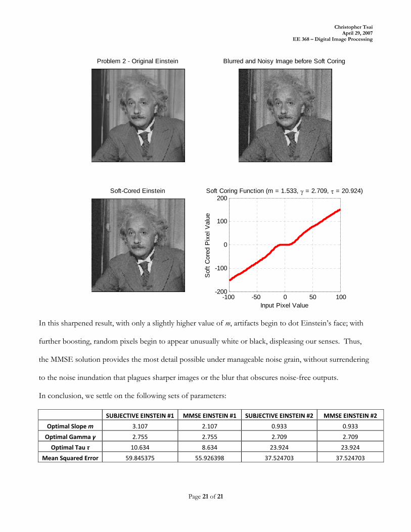
In this sharpened result, with only a slightly higher value of m, artifacts begin to dot Einstein’s face; with

further boosting, random pixels begin to appear unusually white or black, displeasing our senses. Thus,

the MMSE solution provides the most detail possible under manageable noise grain, without surrendering

to the noise inundation that plagues sharper images or the blur that obscures noise-free outputs.

In conclusion, we settle on the following sets of parameters:

SUBJECTIVE EINSTEIN #1 MMSE EINSTEIN #1 SUBJECTIVE EINSTEIN #2 MMSE EINSTEIN #2

Optimal Slope m 3.107 2.107 0.933 0.933

Optimal Gamma γ 2.755 2.755 2.709 2.709

Optimal Tau τ 10.634 8.634 23.924 23.924

Mean Squared Error 59.845375 55.926398 37.524703 37.524703


Soft-Cored Einstein

-100 -50 0 50 100-200

-100

0

100

200

Input Pixel Value

Sof

t Cor

ed P

ixel

Val

ue

Soft Coring Function (m = 1.533, γ = 2.709, τ = 20.924)

problem set iii responsepeople.csail.mit.edu/halordain/digital image processing...christopher tsai...

Documents