problems of world agriculture -...

Scientifi c JournalWarsaw University of Life Sciences – SGGW

PROBLEMSOF WORLD

AGRICULTUREVolume 6 (XXI)

POLISH AGRICULTURE AND FOOD ECONOMY WITHIN THE EU FRAMEWORK

Warsaw University of Life Sciences PressWarsaw 2009

EDITORIAL ADVISORY BOARD Jan Górecki (Institute of Rural Development, Polish Academy of Sciences), Wojciech Józwiak (Institute of Agricultural Economics and Food Economy), Bogdan Klepacki president (WUoLS), Marek Kłodziński (Institute of Rural Development, Polish Academy of Sciences), Henryk Manteuffel (WUoLS), Ludmila Pavlovskaya (State University of Agriculture and Ecology, Ukraine), Wallace E. Tyner (Purdue University, USA), Stanisław Urban (University of Natural Sciences Wrocław), Harri Westermarck (University of Helsinki), Jerzy Wilkin (Warsaw University), Maria Bruna Zolin (Universita di Venezia C’a Foscari) EDITORS Jan Górecki, Zdzisław Jakubowski, Jan Kiryjow, Tomasz Klusek (secretary), Julian T. Krzyżanowski, Henryk Manteuffel Szoege (chief editor), Teresa Sawicka (secretary), Stanisław Stańko, Michał Sznajder REVIEWERS professors Jan Górecki, Julian T. Krzyżanowski, Henryk Manteuffel Szoege, Stanisław Stańko doctors Anna Górska, Mariusz Hamulczuk, Marcin Idzik, Zdzisław Jakubowski, Elżbieta Kacperska, Joanna Kisielińska, Tomasz Klusek, Dorota Komorowska, Paweł Kobus, Dorota Kozioł, Jakub Kraciuk, Elwira Laskowska, Janusz Majewski, Maria Parlińska, Robert Pietrzykowski, Agnieszka Sobolewska, Alicja Stolarska, Ewa Wasilewska Scientific editor: Henryk Manteuffel Szoege Publication subsidized by the Marshall of Mazowieckie Voivodeship

ISBN 978-83-7583-132-0 Warsaw University of Life Sciences Press 166 Nowoursynowska St., 02-787 Warsaw phone(+48 22) 593 55 20, e-mail: [email protected] www.wydawnictwosggw.pl Printed by Agencja Reklamowo-Wydawnicza A. Grzegorczyk, www.grzeg.com.pl

TABLE OF CONTENTS

- Alexander Boldak, Dmitry Rudenko, Maria Pestis, Paul Pestis, Elena Rudenko Agroecotourism development in the Republic of Belarus ........................... 5

- Valda Bratka, Artūrs Prauliņš Diversity of Farm Indebtedness in Latvia and Poland: a Comparative Study .......................................................................................................... 10

- Anatoliy Dibrova, Larysa Dibrova Domestic support for Ukrainian agriculture under the conditions of world financial crisis ............................................................................................ 26

- Jan Górecki, Ewa Halicka Human and social capital in agricultural and rural development (Polish experiences) ................................................................................................ 33

- Katarzyna Gradziuk Development of food industry in Poland in the years 1998-2007 ........... 41

- Paweł Kobus Wheat yields variability in Poland at NUTS 2 level in context of production risk .............................................................................................................. 51

- Henryk Manteuffel Szoege, Agnieszka Sobolewska Life cycle analysis with regard to environmental impact of apple wholesale packaging ................................................................................................... 59

- Anna Sychtevnik, Iosif Degtyarevich, Nellia Degtyarevich Influence of the state support on the efficiency of dairy farms in Byelorussia ............................................................................................. 69

- Emese Szőcs, Boróka Bíró Territorial differences of climate change impact on Romanian crop production .................................................................................................. 74

- Andrzej Tabeau Influence of macro-economic growth, CAP reforms and biofuel policy on the Polish agri-food sector in 2007–2020 .................................................. 88

5

Alexander Boldak1 Dmitry Rudenko2 Maria Pestis3 Paul Pestis4 Elena Rudenko5 Faculty of Economics Grodno State Agrarian University Republic of Belarus

Agroecotourism development in the Republic of Belarus

Abstract. Agroecotourism is becoming the most dynamical branch of the world tourist industry. The Republic of Belarus has inexhaustible potential for the development of agroecotourism. It promotes a steady development of rural regions, raises well-being of its inhabitants by attracting investments, creates modern social infrastructure and new work places, contributes to the achievement of social and cultural purposes. Agroecotourism is considered to be an important component of a successful realization of the ‘State Program for the Revival and Development of the Countryside in the Republic of Belarus for 2005-2010’. The problem is that the agrotouristic enterprises have not enough money to increase the scale of realization of basic concepts and models stipulated by the National Program. Maintaining and developing the natural and human potential of Belarus will require making the agroecotourism a profitable branch of the agrarian sector of economy.

Key words: agroecotourism, development, international tourist trips, Neman region, Augustov canal

Introduction

Tourism has became one of the most profitable and intensively developing branches of the world economy. Tourism expenses make up 12% of the world GDP, 8% of the world export and 30-35% of the world trade in services. For the last 20 years the annual average rates of growth of the international tourism have been up to 5,1%, currency receipts 14%. Experts forecast that this branch of economy will develop at high rates further on. Tourist business incomes are expected to increase up to $ 1,248 billion by 2020 while in 1998 they made up $ 444,7 billion [When … 2004].

According to data of the World Tourist Organization (WTourO) the development of world tourism shows a growing competition among the countries and regions wishing to receive tourists. However, undeveloped material resources of tourism and its infrastructure, information vacuum, absence of objects ready to hold excursions disadvantage the countries wishing to receive tourists.

1 DrSc, head of the Chair of Agricultural Economics. 2 Deputy dean of the Faculty of Economics, e-mail: [email protected]. 3 DrSc, associate professor. 4 Research assistant. 5 DrSc, senior lecturer.

6

Problems of agroecoturism development

The problem of development of tourism in the Republic of Belarus is paid attention to by the government of the country. To turn tourism into a profitable branch of economy is the task the president of the country put to various governing bodies. All ministries and departments involved in tourist activity are working to achieve the goal. The new situation in the development of Belarussian tourism is reflected in the projects of the decree of the president ‘On the state support of tourism in the Republic of Belarus’. This is also reflected in the national program for development of tourism in 2006-2010, in a new edition of the law ‘About tourism’, in decisions and resolutions of local authorities.

It is important to note that tourism is not only companies, tourist agencies but it also comprises a whole sector of economy: hotel business, public catering, industry of entertainments, transportation, household service and many others. The product made by each sphere should meet the world standards developed by WTourO. An essential contribution to the creation of tourist competitive product and to the transformation of tourism into a profitable branch of economy should be made by the state. The national program for the development of tourism in 2006-2010 will be fulfilled if the economic mechanisms stated in the project of the Decree of the President ‘On the state support of development of tourism in the Republic of Belarus’ are implemented and will work efficiently. Adopted at the end of 2000 the national program for development of tourism in 2001-2005 assumed that about 159 billion roubles will be spent for its realization. It was planned that in 2004 tourism incomes would make up to $ 4.637 million; the number of employees in this sphere would increase up to 5889,8; the total tourism revenue would reach $ 36.943 million. Unfortunately, the program was not successful as only 6 billion roubles were awarded from the budget sources and 2 billion roubles from nonbudget sources. At the same time in 2004 the rates of injection of money in development of the infrastructure made 70 % of the 2003 level. In 2005 the volume of investments in the branch increased almost twice and by the end of 2005 the program was executed in almost 70 % [Radiuk 2007].

According to data obtained by WTourO the number of the international tourist trips is growing. Only in 2008 they increased by 20 % in comparison with 2007. Human and natural resources, sights attract foreign tourists. In 2005-2008 the volume of tourist services has grown half as much; the profit growth made up 133.6%. More tourists visit the country. But the problem is that tourists do not hurry to spend their money coming into the Republic of Belarus. In Lithuania the average tourist spends $ 400-500, in Poland $ 700-800. Though on the territory of Belarus there are 15 000 objects of natural, cultural and historical heritage, only 5% of them are used for tourist purposes. But the quality of the tourist product is low, thus it does not meet the requirements of WTourO. So, foreign tourists travelling via Belarus do not stop for a night even in such tourist centres as Myr, Nesvizh, Novogrudok, Turov, Polotsk.

A new edition of the law ‘About tourism’ obliges touristic companies to improve the quality of their touristic products and offers, to improve the obligatory professional certification of guides and guides-interpreters, to enter the names of certificated experts into the appropriate National Register and to refer to tourism as the only business activity of travel agencies and tourist operators, the latter should be only legal persons. The results of a research testify that, in order to organize the work of operators effectively, the staff should comprise not less than 5-6 men. According to the Belarussian legislation a businessman can

7

have no more than 3 employees being his relatives. The law ‘About tourism’ regulates the activity of touristic enterprises more rigidly and determines their duties, registers the mechanism of rendering tourist services, contains paragraphs about the requirements in the quality of services, safety and insurance in the sphere of tourism, imposes the responsibility for defaults or inadequate execution of functions, which under a contract are carried out by a third person, on the touristic service contractor.

To stimulate development of tourism in the near future it is necessary to solve a number of problems:

• to improve an entrance and internal visa customs regulations; • to eliminate price discrimination in hotels; • to certify the quality of hotel services; • to develop and to fulfil a marketing program for development of tourism; • to accomplish the improvement of 26 tourist zones; • to maintain the state financial support for development of tourism in the initial

period as a sector of national economy; • to distribute high quality booklets with the description of Belarusian tourist

products through international tourist firms and operators; • to buy space in the international foreign exhibitions for accommodation of

Belarusian tourist advertisements, as the lack of information is an obstacle for those who want to have a rest in Belarus.

Some of the factors restraining development of this branch has already been eliminated. Visa prices for the US citizens are reduced, the procedure of reception of two and three-term visas is simplified, the principle of "one window " at the border is put into force ,etc. In order to assist in formation of the Belarussian image as a region attractive for development of tourism and in promotion of the national touristic product in the external market the Chamber of Representatives of the country ratified the Charter of WTourO. Being a member of this organization, Belarus will take advantage of the valuable experience of WTourO experts in conducting statistical accounting. Besides, the republic will receive access to the expert estimation of the projects directed to creation of a competitive tourist brand of the Republic of Belarus. And finally, there are chances to receive significant financial support which is awarded by international organizations for the reconstruction and restoration of the touristic centres.

The strategy of tourist business in our country should have more definite features. The president’s decree which provides tax privileges for tourist companies contributes much to the development of tourism in the republic. In particular, a touristic concern "Belinturist" plans to construct guest houses in locations endowed with historical and natural sights. Certainly, it will not solve all problems concerning the infrastructure but the business will be set in motion. It is time to create a special fund to which travel companies (652 organizations, 655 tourist operators and 652 tourist agents are engaged in this sphere of activity) would make contributions . For example, in Cyprus tourist operators deduct up to 5 % from their profit and remit it into a special fund. Then the fund council decides how these means should be spent. It had a positive influence on the tourist influx. But it is necessary to lower the level of taxation for this purpose. The decree of the chief of the state provides support for enterprises investing resources in the development of touristic infrastructure, for tax credits, for VAT on building and assembly works which are carried out by contracted and subcontracted organizations during the normal term of construction

8

and reconstruction of objects in the tourist industry. The document stipulates that these privileges concern only those objects which are located along the highways included into the international transportation corridors. Beside the above-stated privileges concern those who erect tourist objects on the territory of such national parks as "Belovezhskaya Preserve", "Braslav Lakes", "Naroch-, "Pripyat- "Beresina State Biosphere Reserve", and also in vicinity of the Belarussian part of the Augustov canal and the cities of Nesvizh, Polotsk, Turov. It is proposed that the document should concern the territory in 26 tourist zones created in Belarus.

In the near future the reconstruction of the Belarusian part of the Augustov canal will be completed which will increase the afflux of foreign tourists in this region. The region is famous for its rich cultural heritage which is located in very picturesque places. The network of village roads provides communication between village settlements with the administrative centre in Sopotskin and other settlements. It creates a certain base for planning the reconstruction of roads to provide service to the flow of tourists connected with the canal and it helps solving the problem of village revival. 2946 men live in the region. To be ready to receive tourists in this country it is necessary to take some actions.

1. To use local mass media in order to involve the village population in touristic services as a source of income and a rise of their standard of living; to involve public organizations, Sopotskin local council, local authorities of Grodno region, tourist and sport organizations of the region in this activity.

2. To complete the construction of village houses whose owners would like to receive tourists. For this purpose it is necessary for the village population to use not only their own monetary resources, but also soft loans.

3. To reduce the requirements for allocation of construction rights to the investors in cafes, bars, restaurants, camping sites, rental and household services, new village houses established at their expense. A reliable legislative base will stimulate an investment activity directed to creation of the tourist product.

4. To revive musical traditions and family folklore, to organize national festivals with tourist participation.

5. To revive activity of the local handicraftsmen: weavers, smiths, potters, embroiderers, artists, and those making things from straw, wicker, wood and to sell the produce in shops, booths, minimarkets located along the Augustov canal by salesmen dressed in national costumes;

6. Special attention should be given to high quality and variety of dishes of the Belarussian cuisine for tourists, to creation of comfortable village houses. To solve this problem it is necessary to employ experts in cooking and housekeeping which are trained in Belarussian colleges.

The practical importance of development of rural tourism in the Neman region is that this branch may become a part of investment sources for reviving the country, an important factor of employment and earnings for village population. It is confirmed by the experience of foreign countries that are not rich in mineral resources but enjoy a high level of social and economic standards thanks to the service industry and first of all to the tourist business. Accommodation of tourists was expected to become a secondary economic activity in Italy, which was a recognized leader in the sphere of tourism, with regard to rising the Italian standard of living. However, today's demand has changed the concept of this activity which became the major one for many rural people [Klitsunova 2008].

9

In the Republic of Belarus there are already more than 500 country houses and manors receiving tourists. Here various services, traditional countryside lifestyle, cultural and material heritage of the Belarussian village and the beauty of rural nature is offered to visitors. It is necessary to mobilize and to use a favourable geographical position of the Neman region, its historical sights and monuments, national parks, reserves, hunting areas, hospitality of the local population, traditions and customs, the national cuisine, Belovezhskaya preserve, the reconstruction of the Augustov canal which are the components of the tourist potential of Grodno region. It will help to create a competitive tourist product supported financially by the state.

Summary

In order to make the agroecotourism a dynamically developing branch it is important to solve such problems as a lack of traditions and experience in receiving tourists, ignorance of foreign languages, weakness and isolation of providers of village tourism services, low level of the tourist staff preparation and of excursion programs, insufficient promotion of the tourist product. For the solution of these problems it is necessary that 30-40% of the investment funds should come from return of taxes to the local budgets paid by the tourists. Companies which are engaged in tourist business, travel companies should be granted tax privileges. It is necessary to use these funds for keeping the traditional workshops with the local owners, for editing high quality promotion materials of tourist products, for training experts in rowing, water cycling, swimming, fishing, hunting, horse riding, foreign languages.

Thus, only an active position of the communes interested in development of tourism will allow to fulfil the task put forward by the chief of state in the Republic of Belarus, to make tourism a profitable branch of the national economy.

References

When entrance tourism becomes business? [2004]. New Economic Newspaper no. 61, p. 1. Radiuk A. [2007]: Belarus ratified the Charter of theWorld Tourist Organisation. New Economic Newspaper no.

37, p. 3. Klitsunova V. [2008]: Tourism with the prefix "Agro". Belarussian dumka no. 12, pp. 36-39.

10

Valda Bratka1, Artūrs Prauliņš2 Department of Farm Economics Latvian State Institute of Agrarian Economics Riga, Latvia

Diversity of Farm Indebtedness in Latvia and Poland: a Comparative Study

Abstract. The use of borrowed capital in Latvian agricultural holdings of different economic size and type of farming is analyzed, as well as a comparative analysis with Polish agricultural holdings is performed, defining essential specificities of financing activities with equity or loan in each state. The liabilities burden in Latvian field crop and dairy farms is calculated and discussed in detail. For the assessment ratio of the statistical significance of differences between Latvian and Polish agricultural holdings the debt-to-equity and total liabilities per ESU, per 1 ha UAA and 1 LU, a statistical testing is carried out and main conclusions about an impact of the type of farming, the economic size and the chronological factor are formulated.

Key words: debt, liabilities, Latvian farms, Polish farms, comparative analysis

Introduction

Agriculture is currently one of the Latvian economy branches to suffer most seriously from the economic recession, essential price fluctuations in the market and the inflation caused price rise. As a result the costs are growing fast, but production the sale prices decrease, tending to drop lower than the product costs. Decreasing revenues hinder repayment of loans by the farmers. In order to relieve the burden of loans a State Support Program for 2009 is supposed to grant an allowance for paying down of actual interest payments by businesses (in case a loan or a leasing was taken to purchase new agricultural machinery and equipment or to construct industrial buildings, etc.), as well as for loan guarantees or for restructuring of existing loans (extension of final date of repayment or loan refinancing) [Par pasākumu… 2009]

According to the Latvian Ministry of Agriculture and a recent information in Latvian press [Latvijā arvien... 2009] big farms are particularly overloaded with credit liabilities, so checking the validity of this statement is topical in this research. The objective of this article is to analyze the use of borrowed capital in Latvian agricultural holdings of different economic size and type of farming and to offer a comparative analysis of Latvian and Polish agricultural holdings, defining essential specificities of activities financed from equity or loan in each state. To achieve this objective, methods of comparative ratio analysis, data grouping and statistical evaluation as well as inductive-deductive reasoning

1 Dr oeconomiae, full member of Latvian Academy of Agricultural and Forestry Sciences, head of department; Struktoru street 14-214, LV-1039, Riga, Latvia; tel. (371) 67552786; e-mail: [email protected] 2 Dr oeconomiae, Magister iuris, assistant professor, researcher; Struktoru street 14-213, LV-1039, Riga, Latvia; tel. (371) 67552786; e-mail: [email protected]

11

are used. All calculations are made by authors and based on data obtained from FADN national liaison agencies3 in Latvia and Poland.

Financial leverage ratios

As agricultural holdings differ substantially not only by production process specificities (e.g. field crops, horticulture, dairy or granivores type of farming), but also by economic size, financing policy, level of investments and other factors, it is rather difficult to elaborate a general method of agricultural holdings’ solvency analysis. Though the ratio analysis is the most widespread express method4 both for solvency and creditworthiness assessment (especially, if detailed analysis is not possible due to lack of data), it must be taken into account that this method has a number of disadvantages. Most important of them are the following [Zelgalve 2004]:

1) orientation to past experience and a limited ability of making future forecasts; 2) assessment statics, a limited ability to run an analysis of the financial position of

agricultural holding as of a continuously functioning enterprise, mostly done for a certain moment of time instead;

3) inability to define the amount of potential loan, necessary to achieve the maximum efficiency in the borrower’s business activity.

Financial leverage ratios are used to assess how much financial risk a farm has taken on. There are 2 types of financial leverage ratios [Fabozzi 2003]: component percentages (comparing a farm’s debt with either its total capital, i.e. debt and equity, or its equity capital) and coverage ratios (reflecting a farm’s ability to satisfy fixed financing obligations, i.e. interest, principal repayment, or leasing payments). Neither practical nor scientific papers agree about which component percentage ratio is more preferable for the analysis of solvency. For example, in a financial analysis practitioner’s guide [Guide… 2003], a debt-to-equity ratio (total liabilities/equity) and a financial leverage ratio (share of a company’s long-term debt in its capital structure) are mentioned. In another handbook [How… 2000] just a debt-to-equity ratio is included. Some authors [Siegel 1995] call the above mentioned ratio also as a debt to net worth ratio. It is argued [Kohler’s… 1983] that the debt-to-equity ratio is normally calculated by dividing total liabilities by total equities5 or total assets. At the same time many other versions are used: some analysts prefer long-term debt as the numerator, others consider long-term equity or just stockholder’s equity as the denominator. Historically, the debt-to-equity ratio was called the leverage ratio. While the debt-to-asset ratio is used extensively in the press, the leverage ratio has historical importance and is still used by many analysts in the financial sector [Olson 2004; Penson 3 The EU Commission does not collect data directly. So called FADN liaison agencies (for example, Latvian State Institute of Agrarian Economics in Latvia and Institute of Agricultural and Food Economics in Poland) are responsible for gathering accountancy data from farms for he aims of determination of incomes and business analysis of agricultural holdings. 4 According to Kovalov [Kovalov & Volkova 2009] the sequence of the so called express financial analysis performance is: 1) formal examination of the content of financial statements, 2) acquaintance with auditor’s report, 3) disclosure of „problematic” items and their dynamics, 4) analysis of company’s published key ratios, 5) acquaintance with notes to the financial statements, 6) approximate evaluation of company’s activity, solvency and financial position using ratio analysis, 7) formulation of conclusions. 5 Hereinafter the terminology of Kohler’s dictionary [Kohler’s… 1983] and other cited references is retained without modification.

12

1982]. Nowadays the debt-to-equity ratio is extensively used in multi-factor models. For example, it is so in an eight factor model6 (modified Du Pont model) elaborated by Erohin [2007] to determine which of the elements is dominant in any change of farm ROA, effective use of financial resources and financial stability. Bocharov [2005] denotes the proportion of total liabilities and equity as a ratio of financial dependence (коэффициент финансовой независимости), their inverse proportion as a ratio of financing (коэффициент финансирования), a proportion of total liabilities to total assets as a ratio of financial stress (коэффициент финансовой напряжённости).

Earlier research papers [Bórawski 2008; Jakušonoka 2007; Kotāne 2008] analyzed Latvian and Polish agricultural holdings solvency by relating long-term or total liabilities only to values in terms of money (such as total assets, equity etc.). In this article the method has been modified, using the following money values and physical units as allocation base7 of total liabilities:

a) financial indicator (equity); b) production resource, 1 hectare of utilized agricultural area (hereinafter UAA 1 ha)

and livestock unit (hereinafter LU); c) production output; European size unit (hereinafter ESU).

Comparative analysis of liabilities burden in Latvian and Polish farms

Researchers [Herczeg 2009] mention the lack of capital and low level of capital accumulation in agricultural holdings as main reasons for increased need for external financial resources. Erohin [2007] is of the same opinion, putting the accent on an important role of long-term loans in the implementation of new production technologies, a replacement of agricultural machinery, an UAA fertility increase. Along with the growth of Latvian and Polish agricultural holding sizes, also the debt-to-equity ratio was growing (Table 1).

The policy of external capital attraction to financing in Latvian agricultural holdings was more active than in the Polish farms, the biggest risks taken by the big holdings (over 250 ESU), where the share of external capital exceeded 1.4-1.65 times the share of equity. In the end of the analyzed period, comparing to 2002, the debt-to-equity ratio in Poland grew most of all in farms smaller than 16 ESU, but in Latvia in farms of size 8 to 16 ESU and 100 to 250 ESU. For Polish farms the fastest chain growth rate8 of debt-to-equity ratio was observed a year earlier (already in 2003-2004) than in Latvian farms (year 2004-2005). It is necessary to emphasize that in some previous research [Franc 2003] the calculated average debt-to-equity ratio of Polish agricultural holdings (selection of farms from ‘Ranking of 300 best agricultural enterprises’) in 1994-2000 was remarkably higher. It was

6 ROA = (profit / sales) × (sales / current assets) × (current assets / short-term debts) × (short-term debts / accounts receivable) × (accounts receivable / accounts payable) × (accounts payable / total liabilities) × (total liabilities / equity) × (equity / total assets) [Erohin 2007]. 7 By analogy with the allocation base (or cost driver) defined in management accounting as the basis that is used to allocate costs to cost objects [Drury 1994], in this paper it is used for the allocation of liabilities to some parameters of agricultural production (production resource, output etc.). 8 The chain growth rate of time series is a chain growth coefficient which is expressed in percentages and reveals an increase, a decrease or invariability of the current level in comparison with a previous one [Aladjev 2004].

13

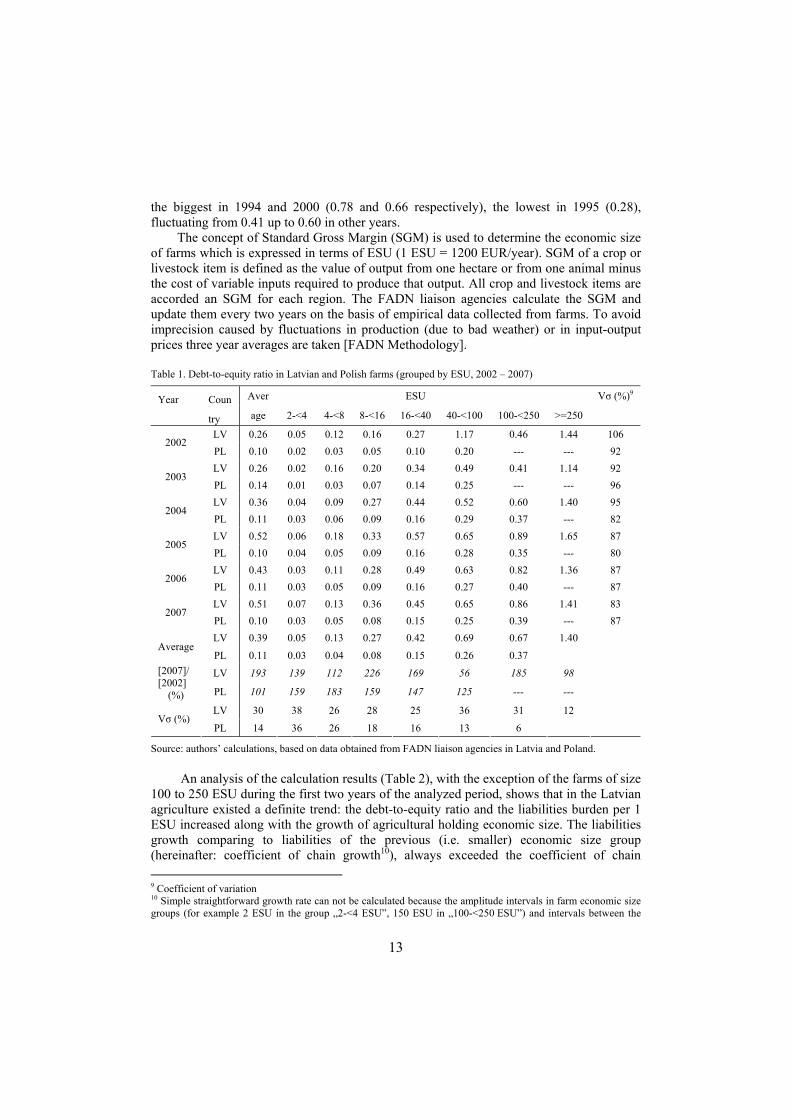
the biggest in 1994 and 2000 (0.78 and 0.66 respectively), the lowest in 1995 (0.28), fluctuating from 0.41 up to 0.60 in other years.

The concept of Standard Gross Margin (SGM) is used to determine the economic size of farms which is expressed in terms of ESU (1 ESU = 1200 EUR/year). SGM of a crop or livestock item is defined as the value of output from one hectare or from one animal minus the cost of variable inputs required to produce that output. All crop and livestock items are accorded an SGM for each region. The FADN liaison agencies calculate the SGM and update them every two years on the basis of empirical data collected from farms. To avoid imprecision caused by fluctuations in production (due to bad weather) or in input-output prices three year averages are taken [FADN Methodology].

Table 1. Debt-to-equity ratio in Latvian and Polish farms (grouped by ESU, 2002 – 2007)

Year Coun Aver ESU Vσ (%)9

try age 2-<4 4-<8 8-<16 16-<40 40-<100 100-<250 >=250

LV 0.26 0.05 0.12 0.16 0.27 1.17 0.46 1.44 106 2002

PL 0.10 0.02 0.03 0.05 0.10 0.20 --- --- 92 LV 0.26 0.02 0.16 0.20 0.34 0.49 0.41 1.14 92

2003 PL 0.14 0.01 0.03 0.07 0.14 0.25 --- --- 96 LV 0.36 0.04 0.09 0.27 0.44 0.52 0.60 1.40 95

2004 PL 0.11 0.03 0.06 0.09 0.16 0.29 0.37 --- 82 LV 0.52 0.06 0.18 0.33 0.57 0.65 0.89 1.65 87

2005 PL 0.10 0.04 0.05 0.09 0.16 0.28 0.35 --- 80 LV 0.43 0.03 0.11 0.28 0.49 0.63 0.82 1.36 87

2006 PL 0.11 0.03 0.05 0.09 0.16 0.27 0.40 --- 87 LV 0.51 0.07 0.13 0.36 0.45 0.65 0.86 1.41 83

2007 PL 0.10 0.03 0.05 0.08 0.15 0.25 0.39 --- 87 LV 0.39 0.05 0.13 0.27 0.42 0.69 0.67 1.40

Average PL 0.11 0.03 0.04 0.08 0.15 0.26 0.37

LV 193 139 112 226 169 56 185 98 [2007]/ [2002]

(%) PL 101 159 183 159 147 125 --- ---

LV 30 38 26 28 25 36 31 12 Vσ (%)

PL 14 36 26 18 16 13 6

Source: authors’ calculations, based on data obtained from FADN liaison agencies in Latvia and Poland.

An analysis of the calculation results (Table 2), with the exception of the farms of size 100 to 250 ESU during the first two years of the analyzed period, shows that in the Latvian agriculture existed a definite trend: the debt-to-equity ratio and the liabilities burden per 1 ESU increased along with the growth of agricultural holding economic size. The liabilities growth comparing to liabilities of the previous (i.e. smaller) economic size group (hereinafter: coefficient of chain growth10), always exceeded the coefficient of chain 9 Coefficient of variation 10 Simple straightforward growth rate can not be calculated because the amplitude intervals in farm economic size groups (for example 2 ESU in the group „2-<4 ESU”, 150 ESU in „100-<250 ESU”) and intervals between the

14

growth for an average economic size of respective agricultural holdings group. If in farms in the group of size 16 to 250 ESU the difference in the coefficient growth fluctuated from 0.4 to 0.95 (only in year 2007 in the group 100 to 250 ESU it was 1.15), then in other groups it was from 2.5 to 4 (reaching its maximum of 7.1 in the group 4 to 8 ESU in 2003). In Polish farms the difference between coefficients of chain growth for liabilities and for an average economic size was essentially smaller. In 2002-2003 it ranged from 1.2 to 1.7, in other years from 0.3 to 0.9. A conclusion can be made that in Poland, unlike in Latvia, the growth of liabilities was just a little ahead of agricultural holdings economic size growth.

Table 2. Total liabilities (EUR) per European Size Unit of Latvian and Polish farms (grouped by ESU, 2002 – 2007)

Year Counry ESU Vσ

Average 2-<4 4-<8 8-<16 16-<40 40-<100 100-<250 >=250 (%)

LV 1166 406 675 611 963 2074 1298 2529 65 2002

PL 549 195 188 338 514 768 --- --- 61 LV 1063 177 777 911 1047 1440 1239 2270 57

2003 PL 674 120 211 391 675 945 --- --- 73 LV 1347 294 476 1128 1330 1580 1806 2450 58

2004 PL 624 329 445 529 780 1253 725 --- 49 LV 2163 490 1026 1512 2005 2144 2856 3960 58

2005 PL 644 443 410 558 810 1215 816 --- 43 LV 1852 249 629 1312 1856 1997 2645 3482 65

2006 PL 740 341 425 633 855 1187 1234 --- 49 LV 2073 478 756 1629 1633 2014 3016 3664 61

2007 PL 794 405 477 657 890 1230 1346 --- 47 LV 1611 349 723 1184 1472 1875 2143 3059

Average PL 671 306 359 518 754 1100 1030 671 LV 178 118 112 267 170 97 232 145 [2007]/

[2002] (%) PL 145 208 254 195 173 160 --- ---

LV 30 37 25 32 29 15 37 24 Vσ (%)

PL 13 41 35 25 18 18 30


The use of UAA is quite widespread in economic analysis for comparing not only the economic performance of farms in different countries in general [Simon 2002], but also for a calculation of total assets, equity and the burden of total, long-term and shot-term liabilities per UAA 1 ha [Herczeg 2009A].

The statement that due to a larger economic size the agricultural holdings have a heavier liabilities burden was confirmed when total liabilities per UAA 1 ha (Table 3) were calculated. The differences in these values were most pronounced between the groups of largest and smallest Latvian agricultural holdings in 2006 (1549 EUR and 26 EUR) and in centres of groups are not equal. Therefore the chain growth rate of liabilities and the chain growth rate of allocation base are compared in any two groups independently.

15

2003 (1005 EUR and 19 EUR), the most insignificant difference in 2007 (1663 EUR and 66 EUR). Those differences were substantially greater that those of the total liabilities per 1 ESU value (in 2006 they were 3482 EUR and 249 EUR, in 2003 respectively 2270 EUR and 177 EUR). An opposite tendency was observed when comparing differences between coefficient of chain growth for liabilities, economic size and UAA. The difference between coefficient of chain growth for liabilities and UAA was smaller, showing, that liabilities growth was more connected to UAA, rather than to ESU growth. Still such a conclusion does not refer to Latvian farms over 250 ESU, where the ratio between coefficients of chain growth for liabilities and UAA growth during the first years of the analyzed period was within the range of 6 – 6.8 but in the end it varied from 3 to 3.4. This clearly shows that agricultural holdings attracted external financial resources for implementation of large-scale investment projects. This difference for medium-size agricultural holdings (16 to 100 ESU) was smaller (within the range of 0.3 – 0.9), thus the liabilities growth was most of all balanced with the UAA growth.

Table 3. Total liabilities (EUR) per utilised agricultural area (hectare) of Latvian and Polish farms (grouped by ESU, 2002 – 2007)

Year Country ESU Vσ

Average 2-<4 4-<8 8-<16 16-<40 40-<100 100-<250 >=250 (%)

LV 152 37 72 64 121 285 260 1123 137 2002

PL 275 70 88 176 265 384 --- --- 66 LV 149 19 86 108 144 216 229 1005 131

2003 PL 339 44 97 196 337 523 --- --- 81 LV 224 31 59 170 203 261 343 1292 129

2004 PL 385 142 221 333 594 990 547 --- 66 LV 372 54 132 213 321 358 531 2141 135

2005 PL 365 166 189 326 573 943 687 --- 64 LV 328 26 84 217 311 379 567 1549 116

2006 PL 420 132 199 374 606 907 745 --- 63 LV 435 66 114 288 327 439 695 1663 107

2007 PL 449 163 232 391 623 880 831 --- 59 LV 277 39 91 177 238 323 438 1462

Average PL 372 119 171 299 500 771 703 --- LV 286 179 158 449 271 154 267 148 [2007]/

[2002] (%) PL 163 234 264 223 235 229 --- ---

LV 43 46 30 46 39 26 43 28 Vσ (%)

PL 17 42 37 31 31 33 17


In Polish farms the coefficient of chain growth for liabilities, in most cases, exceeded the UAA coefficient of chain growth only by 1.1 – 1.5 (during the last years 0.9 – 1.3). The difference was even smaller in the group of largest holdings, where it fluctuated from 2.4 (in 2004) to 0.35 (in 2007). This allows to conclude that Polish farmers’ strategy of

16

borrowed capital handling was better adapted to changes in the agricultural production resources (UAA) than in the Latvian agriculture.

By analogy with UAA, LU was chosen as an allocation base of liabilities for the analysis of average results in Latvian agricultural holdings and dairy farms. With growing economic size of Latvian agricultural holdings the total liabilities per 1 LU grew only in holdings smaller than 100 ESU and reached maximum in the group 40 to 100 ESU (Table 4). The liabilities burden in farms over 250 ESU made in turn just 55 % (in 2004) up to 85 % (in 2007) of the level in the previous group. In the group of largest Polish agricultural holdings, as compared with the above, the liabilities burden for 1 LU was smaller only in 2004-2005. In the other years this paradox was not observed and the largest Polish farms had the heaviest liabilities burden. If in 2002-2003 the difference between coefficient of chain growth for liabilities and LU fluctuated from 1.2 to 1.7, then in the following year it diminished and exceeded value 1 only in farms of size 40 to 100 ESU. Along with this by the lapse of time the liabilities growth and the LU growth became more equalized, especially in farms smaller than 40 ESU.

Table 4. Total liabilities (EUR) per livestock unit in Latvian and Polish farms (grouped by ESU, 2002 – 2007)

Year Country ESU Vσ

Average 2-<4 4-<8 8-<16 16-<40 40-<100 100-<250 >=250 (%)

LV 590 162 297 373 672 1819 664 1168 79 2002

PL 446 149 140 252 393 759 --- --- 76 LV 511 62 349 481 751 1252 686 839 60

2003 PL 510 88 150 280 501 725 --- --- 75 LV 715 117 200 646 1026 1752 1353 964 69

2004 PL 474 262 325 377 555 919 798 --- 50 LV 1185 172 495 1086 1335 2361 2425 1683 63

2005 PL 461 352 299 396 567 916 565 --- 44 LV 1019 98 301 658 1226 2373 1807 1515 73

2006 PL 534 264 314 441 603 891 901 --- 49 LV 1293 225 416 969 1186 2043 3531 1709 78

2007 PL 623 322 367 479 681 1081 1236 --- 55 LV 886 139 343 702 1033 1933 1744 1313

Average PL 508 240 266 371 550 882 875 --- LV 219 139 140 260 176 112 531 146 [2007]/

[2002] (%) PL 140 217 262 190 173 142

LV 37 42 30 39 26 22 63 29 Vσ (%)

PL 13 43 36 24 18 15 32


Both in Poland and in Latvia an external financing was used most intensively by agricultural holdings of the same types of farming, namely horticulture, granivores and field crops (Table 5). Still the proportions of assets financing from equity and borrowed capital were different. During the first years of the analyzed period the biggest debt-to-equity ratio was stated for Latvian field crop (0.4 – 0.56) and granivores farms (around 0.8).

17

In further years this value grew fast in horticulture farming. In such farms total liabilities exceeded equity 1.5 – 2 times in 2004 and 2007, while in 2006 they were equal. In granivores farms the debt-to-equity ratio had an average of 1.26 in 2002-2007, fluctuating between 1.2 to 1.7 from year to year, which is considered a very high level of financial risk. The debt-to-equity ratio in Polish holdings of the mentioned type of farming was on average 0.15 – 032, but the biggest did not exceed 0.33 – 0.37 in 2004-2005, which is considered an optimum value from the point of view of financial analysis.

Table 5. Debt-to-equity ratio in Latvian and Polish farms (grouped by types of farming, 2002-2007)

Year Country

Fiel

d ro

ps

Dai

ry c

ows

Gra

nivo

res

Hor

ticul

ture

Mix

ed c

rops

Mix

ed

lives

tock

Mix

ed c

rops

an

d liv

esto

ck

Perm

anen

t cr

ops

Gra

zing

liv

esto

ck

LV 0.56 0.21 0.82 0.21 0.06 0.06 0.07 --- --- 2002

PL 0.15 0.09 0.07 --- --- --- 0.08 0.13 0.11 LV 0.41 0.19 0.79 0.29 0.13 0.04 0.10 0.51 ---

2003 PL 0.17 0.13 0.15 --- --- --- 0.11 0.12 0.18 LV 0.51 0.16 1.23 1.57 0.11 0.11 0.14 1.01 ---

2004 PL 0.11 0.08 0.16 0.37 --- --- 0.06 0.11 0.10 LV 0.66 0.30 1.71 0.79 0.21 0.08 0.24 0.55 ---

2005 PL 0.11 0.08 0.16 0.33 --- --- 0.06 0.10 0.09 LV 0.56 0.30 1.43 1.05 0.08 0.06 0.30 0.33 ---

2006 PL 0.15 0.08 0.17 0.27 --- --- 0.07 0.10 0.11 LV 0.62 0.31 1.60 2.05 0.49 0.06 0.36 0.24 ---

2007 PL 0.13 0.09 0.17 0.30 --- --- 0.07 0.11 0.11 LV 0.55 0.24 1.26 0.99 0.18 0.07 0.20 0.53 ---

Average PL 0.14 0.09 0.15 0.32 --- --- 0.07 0.11 0.12 LV 16 28 31 73 88 33 58 56

Vσ (%) PL 17 24 25 14 26 9 27


Analysis of liabilities burden in Latvian field crop byand dairy farms

Field crops and milk production are still those Latvian agricultural production sectors that form the largest part of agricultural production value (in 2007 it was 27% and 21% respectively) [Vēveris 2008].

Similar to the average liabilities ratios in Latvian agriculture, in the field crop farms they varied substantially depending on the economic size of farms (Table 6). In the years 2003-2004, in the groups of the smallest and the largest Latvian agricultural holdings the differences between debt-to-equity ratio, liabilities burden per ESU and per UAA 1 ha tended to decrease, but in the further years they increased anew, reaching the maximum in 2006. Many creditors think that the loan should not exceed the equity [Bednarskis 1992].

18

Farms over 100 ESU have already reached this limit since the liabilities made 80-90 % of equity. Liabilities burden per 1 ESU also had a tendency to grow along with the growing economic size of agricultural holdings. It decreased only in farms 100 to 250 ESU in 2002-2003, as well as in the groups 4 to 8 ESU in 2004 and 8 to 40 ESU in 2005-2006. Still those exceptions were mostly accidental and could be caused by a non-representative sampling. When compared with total liabilities per 1 ESU, the total liabilities per UAA 1 ha were characterized by bigger coefficient of variation Vσ, demonstrating greater variability of this value in different economic size groups.

Table 6. Debt-to-equity ratio and total liabilities (EUR) per 1 European Size Unit and per utilised agricultural area (ha) in Latvian field crop farms (grouped by ESU, 2002-2007)

Year ESU Vσ

Average 2-<4 4-<8 8-<16 16-<40 40-<100 100-<250 >=250 (%)

Debt-to-equity ratio

2002 0.56 0.35 0.13 0.20 0.30 1.73 0.85 2.39 103 2003 0.41 0.05 0.15 0.13 0.35 0.55 0.64 2.09 125 2004 0.51 0.22 0.07 0.19 0.46 0.57 0.83 1.72 98 2005 0.66 0.02 0.35 0.37 0.49 0.78 1.09 2.00 90 2006 0.56 0.01 0.17 0.19 0.38 0.65 0.92 1.58 99 2007 0.62 0.05 0.10 0.26 0.48 0.62 0.81 1.76 101

Average 0.55 0.12 0.16 0.22 0.41 0.82 0.86 1.93

Vσ (%) 16 120 63 37 19 56 17 15

Total liabilities / ESU

2002 1643 1607 596 706 1116 2500 1433 3165 59 2003 1384 365 646 651 1082 1772 1644 2962 69 2004 1650 1529 342 819 1163 1819 2241 3131 59 2005 2208 151 1610 1594 1376 2105 3203 4059 64 2006 1938 38 983 660 1187 1832 2861 4220 85 2007 2543 456 732 1109 1543 1824 3048 6716 98

Average 1894 691 818 923 1244 1975 2405 4042

Vσ (%) 22 101 54 40 14 14 31 35

Total liabilities / UAA (hectare)

2002 195 107 54 70 133 340 329 750 97 2003 183 35 57 78 129 258 339 689 103 2004 257 125 37 126 175 280 448 757 90 2005 352 14 193 224 229 342 578 972 87 2006 328 4 112 109 204 328 575 992 104 2007 465 82 96 175 279 343 603 1435 111

Average 297 61 92 131 192 315 479 932

Vσ (%) 36 83 62 46 30 12 26 30

Source: authors’ calculations, based on data obtained from FADN liaison agency in Latvia.

19

Table 7. Debt-to-equity ratio and total liabilities (EUR) per 1 European Size Unit and per 1 livestock unit in Latvian dairy farms (grouped by ESU, 2002-2007)

Year ESU Vσ

Average 2-<4 4-<8 8-<16 16-<40 40-<100 100-<250 (%)


2002 0.21 0.00 0.17 0.15 0.18 1.20 0.27 133 2003 0.19 0.02 0.25 0.15 0.34 0.27 0.26 52 2004 0.16 0.02 0.08 0.25 0.29 0.23 0.31 59 2005 0.30 0.07 0.15 0.33 0.70 0.44 0.53 65 2006 0.30 0.04 0.09 0.30 0.68 0.53 0.75 75 2007 0.31 0.05 0.06 0.24 0.47 0.69 0.87 85

Average 0.24 0.03 0.13 0.24 0.44 0.56 0.50 Vσ (%) 28 64 54 31 48 64 53


2002 1078 16 1377 983 595 2929 817 89 2003 926 146 1590 736 1196 836 867 54 2004 881 190 466 1341 1439 994 1275 54 2005 1922 529 1058 1782 3776 2344 2653 58 2006 1706 357 537 1724 3270 2735 3003 65 2007 1369 282 302 1143 1798 2551 2700 73

Average 1314 254 888 1285 2012 2065 1886 Vσ (%) 33 70 60 32 62 44 53

Total liabilities / LU

2002 242 4 281 232 114 743 202 97

2003 215 37 380 134 291 202 207 57

2004 224 51 111 348 365 253 323 55 2005 495 141 266 476 929 601 679 56 2006 544 118 176 522 1030 851 951 65 2007 603 117 139 497 766 1161 1190 74

Average 387 78 225 368 583 635 592 Vσ (%) 46 70 45 43 65 58 70

Source: authors’ calculations, based on data obtained from FADN liaison agency in Latvia.

When analyzing the use of borrowed capital in Latvian dairy farms it was found that in 2003-2006 the debt-to-equity ratio as well as the liabilities burden was growing together with the growth of farm economic size only in agricultural holdings smaller than 40 ESU and over 100 ESU (Table 7). In farms 40 to 100 ESU they decreased in turn by 20-40% of the values in the group 16 to 40 ESU. The growth of dispersion characterized by Vσ revealed during the analyzed period still bigger differences in the attraction of external financing. However, in dairy farms the variability range was narrower than in field crop farms. A more detailed research lets the authors conclude that between the debt-to-equity ratios in farms with size over 250 ESU and below 4 ESU existed the biggest numerical

20

differences (11-17 times) and more moderate between the total liabilities per 1 ESU and per 1 LU (5-10 times).

Statistical evaluation of results

In order to assess the statistical significance of the differences between Latvian and Polish agricultural holdings the debt-to-equity ratio and the total liabilities per 1 ESU, per UAA 1 ha and 1 LU a statistical hypothesis testing has been undertaken [Arhipova 2006].

Table 8. Results of F-Test for equality of two standard deviations (α = 0,05) and T-Test for equality of the mean (α = 0,05) in Latvian and Polish farms grouped by type of farming, by ESU and years

Para- Type of farm

meter Field crops Dairy cows Granivores Horticulture Mixed crops and livestock

Permanent crops


F 14.88 9.49 108.46 247.86 37.69 823.14 F crit 5.05 5.05 5.05 9.01 5.05 5.19 T-test 0.00 0.00 0.00 0.07 0.04 0.04

Type/year A11 B C D E F 2002 2003 2004 2005 2006 2007


F 3.04 9.71 27.04 21.61 51.81 79.56 39.92 3.30 2.91 5.93 4.63 4.89 F crit 5.05 5.05 5.05 5.05 5.05 9.01 6.39 6.39 5.05 5.05 5.05 5.05 T-test 0.04 0.00 0.00 0.00 0.01 0.02 0.26 0.15 0.17 0.08 0.13 0.08


F 1.07 2.12 8.78 9.55 2.16 6.79 7.30 1.83 3.37 7.77 5.61 5.43 F crit 5.05 5.05 5.05 5.05 5.05 9.01 6.39 6.39 5.05 5.05 5.05 5.05 T-test 0.56 0.00 0.01 0.01 0.00 0.03 0.14 0.15 0.16 0.04 0.14 0.11

Total liabilities / UAA (ha)

F 8.07 5.34 1.27 2.78 9.24 0.41 1.73 7.09 6.82 3.21 2.41 1.76 F crit 5.05 5.05 5.05 5.05 5.05 0.11 6.39 6.39 5.05 5.05 5.05 5.05 T-test 0.01 0.02 0.03 0.01 0.01 0.03 0.30 0.23 0.07 0.17 0.16 0.23


F 3.03 1.14 9.61 7.65 10.95 15.72 6.88 2.93 5.82 17.22 10.18 10.25 F crit 5.05 5.05 5.05 5.05 5.05 9.01 6.39 6.39 5.05 5.05 5.05 5.05 T-test 0.06 0.21 0.03 0.01 0.00 0.12 0.36 0.35 0.32 0.09 0.23 0.23

Source: authors’ calculations, based on data from Table 1-5 using Excel functions.

The F-Test for equality of two standard deviations was used to check whether the borrowed capital values variance in the relevant Latvian and Polish agricultural holdings

11 Codes for economic size groups: A ‘2-<4 ESU’; B ‘4-<8 ESU’, C ‘8-<16 ESU’, D ‘16-<40 ESU’, E ‘40-<100 ESU’, F ‘100-<250 ESU’.

21

groups (grouped by type of farming, economic size and year) was equal (H0) or different (H1).

H0: σ12 = σ2

2

H1: σ12 ≠ σ2

2

The calculations indicate (Table 8) that with a probability of P = 95 % H0 can not be rejected (i.e. F < Fcrit) and, along with this, there were no statistically significant differences of the debt-to-equity ratio dispersion between Latvian and Polish smallest farms (smaller than 4 ESU), excluding the years 2002 and 2005. When calculating the total liabilities per 1 ESU, the dispersion degree was equal for farms of size below 8 ESU and over 40 ESU, also in 2003-2004, and so for total liabilities per UAA 1 ha in medium-size farms group (from 8 to 40 ESU), also in the beginning (2002) and in the end (since 2005) of the analyzed period. The dispersion of total liabilities per 1 LU did not differ for farms below 8 ESU and in year 2003.

In order to find out whether the Latvian and Polish farms could be assigned to the same population the Student’s T-test was calculated assuming the two groups had the same mean of debt-to-equity ratio and also for total liability ratios.

H0: μ1 = μ2 H1: μ1 ≠ μ1 With a probability of P = 95 % it was possible to reject the hypothesis H0 (value of T-

test > α, α = 0.05) for the total liability ratios in Latvian and Polish agricultural holdings grouped both by the type of farming (except horticulture) and by the economic size (except for the total liabilities per 1 ESU and 1 LU in the group of the smallest farms). Statistically significant differences were observed. When analyzing the differences between the Latvian and Polish farm total liability ratios in different years (chronological aspect), it could be concluded that they were statistically insignificant (with the exception of total liabilities per 1 ESU in 2005).

Table 9. Results of two factor analysis of variance (α = 0,05) in Latvian and Polish farms

Poland Factor Latvia

No I. ‘2 – < 100 ESU’ No II. ‘2004 – 2007’

F P value Fcrit F P value Fcrit F P value Fcrit


Year 2.163 0.085 2.534 9.947 0.000 2.711 0.443 0.654 4.103 ESU 69.773 0.000 2.421 349.104 0.000 2.866 245.654 0.000 3.326


Year 9.256 0.000 2.534 30.878 0.000 2.711 1.886 0.202 4.103 ESU 46.984 0.000 2.421 209.110 0.000 2.866 28.837 0.000 3.326

Total liabilities / UAA (ha)

Year 4.628 0.003 2.534 9.434 0.000 2.711 1.862 0.205 4.103 ESU 66.253 0.000 2.421 55.73 2 0.000 2.866 216.146 0.000 3.326


Year 5.204 0.001 2.534 33.053 0.000 2.711 3.110 0.089 4.103 ESU 18.292 0.000 2.421 291.326 0.000 2.866 14.991 0.000 3.326

Source: authors’ calculations, based on data from Table 1-4 using Excel function.

22

In order to statistically evaluate the dependence of debt-to-equity ratio and total liability ratios per 1 ESU, per UAA 1 ha and per 1 LU on factors (years and economic size), the two-factor analysis of variance (ANOVA) was performed and hypotheses formulated:

for the economic size factor H0: μ1 ESU = μ2 ESU = μ3 ESU = ... = μ i ESU H1: not all μi ESU are equal

for the year factor H0: μ2002 = μ2003 = ... = μ 2007 H1: not all μi year are equal

As the data on Polish agricultural holdings of economic size 100 to 250 ESU in 2002-2003 was not collected and published, the Polish farms set was divided into 2 subsets for creating 2 adjacent ranges of data: farms of size below 100 ESU in 2002-2007 (No I in Table 9) and farms of size below 250 ESU in years 2004-2007 (No II in Table 9).

Basing on the calculation results (Table 9) it may be said that, with 95% probability, both the Latvian agricultural holding economic size and the chronological factor had a significant influence upon the total liability ratios. When analyzing the chronological factor’s impact on the debt-to-equity ratio it was impossible to reject (F < Fcrit, α = 0.05) the hypothesis H0. The impact of this factor is accepted as statistically insignificant. If in the subset of Polish farms (size below 100 ESU, No I in Table 9) with 95% probability the impact of both factors was determined as significant, the chronological factor had no significant influence upon the ratios (debt-to-equity, total liabilities per 1 ESU, per UAA 1 ha and per 1 LU) in another farm subset (No II in Table 9).

Table 10. Results of two factor analysis of variance (α = 0.05) in Latvian farms

Average

Factor F P value F crit


Year 0.872 0.471 3.072 Type of farming 17.389 0.000 2.488

Field crops Dairy cows

F P value Fcrit F P value Fcrit

Total liabilities / equity

Year 2.354 0.065 2.534 1.163 0.355 2.603 ESU 57.713 0.000 2.421 6.627 0.000 2.603


Year 1.638 0.180 2.534 3.023 0.029 2.603 ESU 19.012 0.000 2.421 6.562 0.001 2.603

Total liabilities / UAA (ha) Total liabilities / LU

Year 3.718 0.010 2.534 4.670 0.004 2.603 ESU 52.518 0.000 2.421 6.190 0.001 2.603

Source: authors’ calculations, based on data from Table 5-7 using Excel function.

A two-factor analysis of variance in Latvian farms (Table 10), grouped by type of farming and years (Table 5), as well as in Latvian field crop (Table 6) and dairy farms (Table 7), grouped by years and ESU, reveals that in certain cases the impact of chronological factor was insignificant. When analyzing the impact of this factor on the

23

debt-to-equity ratio, as well as on total liabilities per 1 ESU in field crop farms, the hypothesis H0 could not be rejected with 95% probability. Such factors as the type of farming as well as the economic size of farms should be considered as significantly influencing the analyzed ratios.

Proposals

The community-supported agriculture is a socio-economic mode of agriculture and food distribution. Although it is very popular all over the world12, it is widespread neither in Latvia nor in Poland. Groups of consumers and farmers form cooperative partnerships which usually focus on a system of weekly delivery or pick-up of vegetables and fruit, a type of a vegetable box, sometimes also dairy products and meat to the consumers. The system has many variations in the farm budget support by the consumers. By providing a guaranteed market through prepaid annual sales at the beginning of the production process (mostly in spring), consumers essentially support and help to finance farming operations, reducing the required amount of borrowed capital.

During summer months some farmers receive subsidies (less favorable area, direct and decoupled payments), which form an important part of their gratis financial sources, from the state budget and the European Agricultural Guarantee Fund. A transfer of the time f payments to the spring would significantly improve the inflow of highly necessary resources before the start of agricultural production process and partly reduce the attraction of short-term loans for the current assets acquisition. An increase of the amount of subsidies to interest repayments could also unburden and help farmers with repayment of loans. However, the economic crisis has a negative impact on the state budgets both in Latvia and in Poland and therefore the sums available for allocation to the support of agriculture.

Conclusions

Along with the growing economic size of Latvian and Polish agricultural holdingsan the share of external borrowed capital aimed at increasing the farms performance also increased. The borrowed capital was widely used in field crop, granivores and horticulture farms. Latvian farmers used borrowed capital more actively than Polish farmers, thus taking bigger financial risk (especially the farms of size over 250 ESU). The introduction of community-supported agriculture, the transfer of subsidies (less favorable area, direct and decoupled) payment time from summer to spring and an increase of interest subsidies could improve the well-timed inflow of resources, unburden farmers and reduce the required amount of borrowed capital.

The differences between the coefficient of chain growth of liabilities and of farms average economic size and of average UAA in Latvian farms were bigger than in Polish

12 For example, AMAP (Association pour le maintien de l’agriculture paysanne) in France, Landwirtschaftsgemeinschaftshof in Germany, ASC (Agriculture soutenue par la communauté) in Canada, CSA (Community supported agriculture), Reciproco in Portugal, Teikei (��) in Japan etc.

24

ones. This reveals that Polish a strategy of the borrowed capital handling better adapted both to changes in agricultural output (measured in ESU) and resources (UAA).

The assessment of the statistical significance (α = 0,05) of results in the Latvian and Polish agricultural holdings comparative analysis shows that there existed significant differences in the two states between the debt-to-equity ratios and between the total liabilities per 1 ESU, 1 hectare of UAA and 1 LU in farms grouped both by types of farming and by economic sizes. Such factors as the economic size and the chronological aspect (years) significantly influenced the Latvian agricultural holdings liabilities ratios (except for the chronological factor’s impact on debt-to-equity ratio). While the impact of the two above mentioned factors on Polish smaller farms (size below 100 ESU) subset was significant, then for the farms subset concerning years 2004-2007 the impact of chronological factor was statistically insignificant.

References

Aladjev V., Haritonov V. [2004]: General Theory of Statistics. Fultus Corporation, Palo Alto. Arhipova I., Bāliņa S. [2006]: Statistika ekonomikā un biznesā. Datorzinību centrs, Rīga, (in Latvian). Bednarskis L., Paupa V. Vaikulis J. [1992]: Finanšu pārskatu analīze. Latvijas Universitāte, Rīga, (in Latvian). Bocharov V. V. [2005]: Kompleksnij finansovij analiz. Piter, Saint Petersburg, (in Russian). Bórawski P. [2008]: Analiza wskaźników płynności i zadłużenia indywidualnych gospodarstw rolnych. Problemy

Rolnictwa Światowego, No 4 (XIX), ss. 75-82, (in Polish). Drury C. [1994]: Management and cost accounting. Chapman & Hall, London. Erohin S. M. [2007]: Upravlenie vosproizvodstvom resursov selskohozajstvennih predprijatij v uslovijah

dostupnosti zaemnogo kapitala. Avtoreferat dissertaciji na soiskanije uchenoj stepeni kandidata ekonomicheskih nauk. Orlovskij gosudarstvennij agrarnij universitet, Orel (in Russian).

Fabozzi F. J., Peterson P. P. [2003]: Financial Management and Analysis. John Wiley & Sons, New Jersey. FADN Methodology. Defining the field of observation.

[Available at:] http://ec.europa.eu/agriculture/rica/methodology1_en.cfm#dotfoo. [Accessed 2009]. Franc J. [2003]: Changes in Capital’s Structure in Polish Agricultural Enterprises in the Years 1994-2000,

Proceedings of international conference ‘Agricultural Economics, Rural Development and Informatics in the New Millennium’ (April 01-02, Debrecen, Hungary). [Available at:] http://www.avacongress.net/ava2003/cd/pdf/D346.pdf. [Accessed 2009].

Guide to Understanding Financial Reports. [2003]. A. Fakahany (ed.). Merril Lynch, Addison. Herczeg A. [2009]: Determining the optimal capital structure by agricultural enterprises, Proceedings of

international conference «3th MACE conference ‘Multi-level Processes of Integration and Disintegration’ (January 14-15, Berlin) [Available at:] http://www.mace-events.org/4293-MACE/version/last/part/19/data/?branch=main&language=en. [Accessed 2009].

Herczeg A. [2009A]: Analyse the financial structure of agricultural enterprises in 2002-2006, Proceedings of international conference ‘4th Aspects and Visions of Applied Economics and Informatics’ (March 26-27, Debrecen, Hungary), pp. 661-666. [Available at:] http://www.avacongress.net/pdf/41.pdf. [Accessed 2009].

How to Read a Financial Report. [2000]. Merril Lynch Response Centre, New Brunswick. Jakušonoka I. [2007]: Research of Capital Structure in Agricultural Companies in Latvia, Economic Science for

Rural Development, no 14, pp. 27-35. Kohler’s Dictionary for Accountants. [1983]. W. W. Cooper, Y. Ijiri (eds.). Prentice-Hall, Englewood Cliffs. Kotāne I. [2008]: Latgales reģiona lauksaimniecības finanšu resursi, Opportunities and Challenges of National

Economic Development (conference proceedings, April 17), Rēzeknes augstkola, Rēzekne, pp. 213-223, (in Latvian).

Kovalev V. V., Volkova O. N. Finansovij analiz. Logika ekspress analiza finansovoj otchetnosti. [accessed 2009]. [Available at:] http://www.financial-analysis.ru/methodses/metAFOFinancialAnalysisLogic.html

Latvijā arvien vairāk lielo saimniecību nomoka lielo kredītu slogs (21.03.2009), (in Latvian). [Available at:] http://www.nozare.lv/nozares/agro/item/200903210917250318B4E2B2A849D4A1/. [Accessed 2009].

25

Olson K. D. [2004]: Farm Management. Principles and Strategies. Iowa State Press, Ames. Par pasākumu ieviešanu ekonomikas aktivizēšanai lauksaimniecības, meža, pārtikas un zivsaimniecības jomās.

[Available at:] http://www.zm.gov.lv/doc_upl/Par_pasakumiem_ekonomikas_aktivizesanai_14_01_2009.pdf. [Accessed 2009].

Penson B. J., Klinefelter D. A., Lins D. A. [1982]: Farm Investment and Financial Analysis. Prentice Hall, Englewood Cliffs.

Siegel J. G., Shim J. K. [1995]: Dictionary of Accounting Terms. Barron’s Educational Series, New York. Simon F., Novák J. [2002]: The evaluation of economic situation and comparison of Czech and French

agricultural enterprises, Agricultural Economics, no 48 (9), pp. 389-394. Vēveris A., Krieviņa A. [2008]: Latvijas lauksaimniecības ekonomiskais kopaprēķins (2007-2008). LVAEI

Pētījumu rezultāti, no. 1 (19). LVAEI, Rīga. Zelgalve E. [2004]: Kredītspējas novērtēšana, Latvijas Universitātes Raksti, Ekonomika III, no. 671, pp. 431-438.

26

Anatoliy Dibrova1 State Regulation Department National University of Life and Environmental Sciences of Ukraine Kyiv, Ukraine Larysa Dibrova2 World Agriculture and Foreign Economic Activity Department National University of Life and Environmental Sciences of Ukraine Kyiv, Ukraine

Domestic support for Ukrainian agriculture under the conditions of world financial crisis

Abstract. In the last years Ukraine has allocated considerable, with respect to their load on the budget, financial resources for agricultural support. However the significant increases of budgetary support do not substantially influence the effectiveness indices nor agricultural yields. Such information testifies to an imperfect nature of the internal support mechanism of Ukrainian agriculture. As the result, the domestic support did not become an effective stimulus for a production quality increase nor for a rise in the stock breeding production. In 2008 Ukraine gathered the biggest grain harvest. Increased production did not improve the financial results of agriculture and did not produce a stable and dynamic branch development because of the negative influence of world finance crises. Unbalanced supply and demand for agricultural production, low buying ability of inhabitants, lack of branch effective mechanism of domestic support caused complications of price situation in the domestic food market. Key words: domestic support, agrarian policy, agriculture, Ukraine.

Introduction

An impartial necessity of the state support of agriculture in the conditions of market economy is caused, from the point of view of economic theory, by unique peculiarities which are immanent for this branch, its place and importance in providing the state food security and for the life of society. According to the foreign and national experience the negative consequences of volatility of the internal and external environment have a significant influence on the parameters of agricultural production development. The existing problems are significantly complicated by the crisis phenomena which periodically emerge in the development of the domestic and world economy. It is really true: the global food crisis has been changed by the financial crisis. The scientific research concerning the increase of role and place of the state in the area of regulation of economic processes needs deepening in order to avoid the possibility of appearance of crisis phenomena and in order to provide sustainable agricultural development in the long term.

The complexity of the present situation lies in that for the years of reforms Ukraine has not been able to substantially increase the effectiveness of agricultural production, to perform a technological re-equippment and to create an innovational model of the

1 Doctor of economic sciences, associate professor, Heroyiv Oborony St. 11, Kyiv, 03041, Ukraine, tel. (+38044) 527-86-48, email: [email protected] 2 PhD, associate professor, head of department, Heroyiv Oborony St. 11, Kyiv, 03041, Ukraine, tel. (+38044) 527-86-51, email: [email protected]

27

development of the branch. The managerial decisions of the state in the area of agricultural production are in practice not consistent and effective which, as a result, does not allow to achieve the desirable financial and economic results of the development of the branch and which also does not allow to meet in the full extent the requirements of society. This situation, from our point of view, is caused by a quick change of the external environment, by an absence of practical experience in the decision-making under market conditions, by an insufficient level of its scientific support. It shows that an integrated system of state regulation of agricultural production in Ukraine has not been formulated yet.

Ukraine is making only the first steps as a competent member of the World Trade Organization and that is why it can be affirmed that the degree of its integration into the world markets is not high enough and that the external crises have rather a somewhat lesser influence on the branch than its internal problems. In the future situation, under the conditions of strengthening of the world prices influence on the domestic agricultural market, one of the important tasks of state regulation will be to provide the information on the possibility of appearing of crisis phenomena and to minimize the influence of negative consequences on the Ukrainian economy. Otherwise there arises a real menace for the domestic agriculture which is linked with the possibility of gaining the status of a resource base country for the developed countries.

So there is a necessity of implementation of a weighed and systematic approach to the development and realization of the state agricultural policy, which is directed to the protection of the domestic market with the help of mechanisms which correspond to the international principles and standards; and there is a necessity of formation of a competitive, export oriented agricultural production through an effective usage of land, labour, intellectual, material and financial resources, through an implementation of innovation, increase of labour efficiency and products’ quality and also through the creation of favourable conditions for attraction of state and private investment into the Ukrainian agriculture. The accomplishment of the above tasks will depend on the effectiveness of the state support for the branch on various hierarchical levels of governance.

The theoretical reinterpretation and the methodological improvement of the governmental support for agricultural production under the conditions of global changes of the external environment are caused, first of all, by the need of a quick adaptation of the agricultural branch to the new conditions of economic activities and of a formation of preconditions for a sustainable development of agriculture in the long-term perspective. That’s why the search of new theoretic, methodological and practical approaches concerning the improvement of state support for agricultural production (also taking into account the knowledge which is accumulated by the economic science and also taking account of advanced foreign and national experience) is an exceptionally topical task [Dibrova 2008].

Material and methods

The present research is based on general scientific methodology. During the process of research the system analysis and synthesis, monographic, abstract, logical, economic mathematical, computational and balance methods of scientific research were used.

In order to evaluate the effectiveness of agricultural policy and the level of domestic support for agriculture a methodology which is applied in the OECD member states was

28

used. The methodology of quantitative estimation of the state support is substantiated in the works of such famous scientists as Josling [1988], Tsakok [1990], Webb, Lopes and Penn [1990].

Results

Integration of Ukraine into the world community causes the necessity of a system approach to the analysis of modern processes of the agricultural production development, with the aim of elaboration of appropriate mechanisms of regulation which are able to provide quick adaptation of the agricultural branch into the new conditions of economic activity. Amongst them a special place belongs to justification of theoretical and methodological principles of the state support for agriculture. The important point for the further research is the statement that the state support can not be associated with state regulation, because the latter can be directed not only to the stimulation of development of economic processes, but also to their restriction. The examples of production restriction in agriculture are the programs which are applied in the EU member states and in the USA. Thus, realizing the function of restriction, the state can at the same time exert an incentive influence through the system of governmental support.

In our view, the state support is a constituent of a system of state regulation of agriculture and it is an aggregate of law, financial, economic, organizational and other measures taken by the state (government) within the frames of an incentive influence on the development of both agricultural production and rural areas in the socially desired direction. Nevertheless, treating of state support only from the perspective of financial and budgetary support is incomplete, because it can include an information support, a development of extension service, a system of insurance and exchange market [Dibrova 2008].

Together with this, the modern agricultural economics science requires further research concerning the estimation of effectiveness of state support for agriculture. An investigation of foreign experience shows that in the developed countries changes in producers’ and consumers’ surpluses are widely employed means for measuring (in monetary equivalent) of profit and expenses which appear as a result of a change in country’s agricultural policy. It’s necessary to highlight that in the countries belonging to the Organization of Economic Cooperation and Development (OECD) a significant experience has been accumulated and a methodology and indexes of estimation of the effectiveness of state support of agriculture have been developed. That is why under the conditions of WTO membership an estimation of constructive indices of the state support for agriculture in Ukraine is an urgent task for adaptation of the national regulation system to international requirements.

WTO requirements underscore the need of decreasing the domestic support in that part, which makes distorting influence on trade, and displacing accents from production support to the support of agricultural producers through so called decoupling. However, the level of agricultural support in the countries with developed market economy stays high.

On the average in Ukraine the relative index “Producer Support Equivalent” (PSE) was for 2001-2006 equal to 0.1%, which is much less than in other developed countries of the world. PSE index shows the share of transfers to agricultural producers in the general volume of earnings in agricultural enterprises, or the share of their earnings connected with

29

the state agrarian policy. This attests that on the average 99.9% of gross volume of earnings of agricultural enterprises in 2001-2006 was received from the market without any state support. However, on the other side, there is a question, how is it possible, when in the last years the state has significantly increased the volume of financial resources in support for domestic agriculture. From 2000 to 2006 the volume of state assignments to financing agriculture from the state budget increased more than 6.6 times, from 1.2 to 7.9 billion hryvna. The share of budget assignments to agriculture in general expenses of the state budget increased during the analyzed period from 3.5% to 5.7%, and the same in GDP increased from 0.7% to 1.5%. First of all, such inconsistency is connected with a situation, when simultaneously with the increase of volume of state support took place a significant decrease in purchase price of agricultural products.

In the conditions of market economy for the development of a balanced agrarian policy it is very important to determine correctly its effectiveness and its impact on those who produce agricultural production. With this purpose in mind the “Market Price Support” (MPS) is calculated basing on the “Methodology of state agricultural support appraisal” which has been developed and used in the OECD. It determines the cash value of transfers to producers from consumers and taxpayers for a period of one year, which appeared as a result of action of the state policy instruments and which creates a gap between prices of particular kind of agricultural products in the local and foreign market (Figure 1).

Source: [Methodology… 2009]

MPS indicator is determined in producer’s prices and is calculated according to a formula:

MPS =(Pp - Pw)*S2 where:

S D

a

b c

d

f

g

Q

P

Pp

Pw

S´ D´

D2 D1 Figure 1. Market Price Support (MPS) and transfers to producers from taxpayers (ТВabfg) and consumers (ТВdcfg) in the conditions of export

S1 S2

Transfers to producers from consumers (ТВdcfg)

Transfers to producers from taxpayers (ТВabfg)

Market Price Support (MPS)

30

Pp – local price per unit of product, Pw – world price per unit of product, S2 – local market supply, D2 – local market demand, S1 – local market supply at world prices, D1 – local market demand at world prices.

This approach is based on the fact, that every deflection of local prices from world prices can be treated as an indicator of state intervention into the open market mechanism. The size of price deviation determines the level of this intervention, and, accordingly, gives a quantitative characteristic of state agrarian policy [Melyukhina & Serova 1996].

Figure 2. "Nominal Protection Coefficient" (NPC) and "Market Price Support" (MPS) for wheat producers in Ukraine per 1 ton of grain

-125,3

90,7

25,2

-43,1

76,6

-33,5

215,7

17

-90,8

-4,3 -3,1

2,04

0,850,991,04

1,51

0,900,99

1,19

0,82

1,19

0,57

-150

-100

-50

0

50

100

150

200

250

1996 1997 1998 1999 2000 2001 2002 2003 2004 2005 2006

hrv.

0

0,5

1

1,5

2

2,5

inde

xes

«MPS» for wheat producers in Ukraine per 1 ton of grain, hrv. «NPС» for wheat producers in Ukraine, indexes

Source: own calculation on the base of the OECD data and data of the State Committee of Statistics of Ukraine.

As we see from the data in Figure 2, MPS index for wheat producers in Ukraine for the period from 1996 to 2006 has either positive or negative values, which suggests some inconsistency of the state support system. When this value is positive, the agrarian policy is directed towards agricultural producers support by consumers and state. When this value is negative producers’ incomes are reallocated to consumers’ and other economic groups’ good.

The computed values of NPC (net protection coefficient) index for wheat (as a ratio of average price which producer receives in the local market to the producer’s price in the world market) confirm a price instability and a low effectiveness of the mechanism of state regulation of grain market in Ukraine.

The analysis confirmed that the gross transfers to wheat producers from taxpayers have accounted on the average for 33 hrv per 1 hectare of harvested area in years 2004 –

31

2006. At the same time the gross transfers from consumers have accounted for minus 73 hrv per hectare. Notably, when calculating the average per 1 hectare of agricultural area the commodity producers in fact ‘grant’ the consumers of particular products. In such a way, as a result of a negative value of the MPS index, the state financial resources are actually directed to producers’ compensation (Figure 3).

33,0

-73,0

11,6

-25,6

-80

-60

-40

-20

0

20

40

hrv.

1 hectar 1 ton

Figure 3. Gross transfers to wheat producers from taxpayers and consumers in Ukraine on the average per 1 hectare of harvetsed area and 1 ton of grain for a period 2004-2006, hrv.

Gross transfers to wheat producers from taxpayers, hrv Gross transfers to wheat producers from consumers, hrv

Source: own calculation on the base of the Ministry of Agricultural Policy of Ukraine data and data of the State Committee of Statistics of Ukraine

On the base of conducted analysis we can make a conclusion that capabilities for improvement of the state regulation mechanism are strongly restricted. The need of changing the approach to the mechanism of state regulation is caused by a need of improving the socio-economic parameters of agricultural development and that of formation of the whole system of state regulation with the aim of prevention of a possibility of appearance of crisis phenomena and of minimizing the influence of negative agricultural results on the economy of Ukraine.

So far, in the situation of current level of agricultural productivity portrayed by the calculated indices, the possibility of its development will be insufficient for improving the standards of living of population, guaranteed meeting the food demand and balanced resumption of branch resource potential. That is why without structural reforms, improvement of pricing system and only at the expense of increasing the volume of state support it will be incredibly difficult to solve this problem.

So far the domestic experience brings a confirmation that even substantial increasing the volume of financial resources transfer to agriculture does not give the desirable productive return and the needed increase in provision of products.

32

Discussion

In such a way we can make a conclusion that existing pricing system in makes it impossible to realize expanded reproduction processes in the branch and that the system of state support only partly compensates not fully satisfying receipts from market sale. The analysis testifies that existing market prices do not correspond to the objective needs of producers, taking into account the needed level of equivalence of exchange and of reinvestments in production assets. In the analysis we should avoid using criteria connected with a comparison of support per hectare. When the pricing mechanism is imperfect such support will compensate not fully the lack of receipts from production realization. The commodity producers will not be able to renew their production potential to the level needed for balanced development. We suppose that an improvement of state regulation of agricultural production should be made with taking into consideration its complexity. In particular an improvement is needed of the system of price regulation in agricultural production and of the system of state support of the branch.

Literature

Dibrova A. D. [2008]: State Regulation of Agricultural Production: theory, methodology, practice. Kyiv, pp. 488. Josling T. E. [1973]: Agricultural Protection: Policy and International Trade. FAO, Rome, pp. .82. Tsakok I. [1990]: Agricultural Price Policy: A Practitioner’s Guide to Partial–Equilibrium Analysis. Webb A. J., Lopes M., Penn R. [1990]: Estimates of Producer and Consumer Subsidy Equivalents. Government

Intervention in Agriculture. Melyukhina O., Serova E. [1996]: Estimating the Level of State Support of the Agrarian Sector: Adaptability of

Conventional Methods in the Transitional Economy. Вопросы экономики, no. pp. 102. Methodology for the measurement of support and use in policy evaluation. [Available at]:

www.oecd.org/dataoecd/36/47/1937457.pdf. [Accessed May 2009].

33

Jan Górecki1 Institute of Rural and Agricultural Development Polish Academy of Sciences Ewa Halicka2 Faculty of Human Nutrition and Consumer Sciences Warsaw University of Life Sciences Warsaw

Human and social capital in agricultural and rural development (Polish experiences)

Abstract. Authors define and explain the meaning of two concepts, namely human and social capital and their influence on the socio-economic progress in agriculture and rural areas. The presented studies and analyses point to the link between the growing role of these two factors and the general socio-economic progress. A major part of the paper is devoted to analysing the past and current state of human and social capital in Poland, focusing on their deficiencies and the need to improve their quality. In conclusion the authors note that the significant inflow of financial means after the the Polisj accession to the EU as well as structural and administrative changes will not bring in full the possible benefits in the future unless there is an improvement in quality and an increase of creative participation of the human and social capital. The health aspect is also explored in the paper as a crucial element influencing human capital in the Polish rural areas.

Key words: human and social capital, development of agriculture and rural areas, health

Main concepts and their evolution

Historically speaking, an agricultural farm and agriculture were defined as a unit of three factors: nature, labour and capital. As a result of progress, i.e. an increase of intensity and productivity but also a development of horizontal and vertical ties, the labour factor started to play a leading role, especially in management, which deals with organising and managing all production factors. This in turn, when used efficiently, brings bigger and better effects in farming and improves the standard of living. The factor responsible for the efficiency of organisation and its effects was distinguished and called human factor or human capital in agriculture. The significance of this factor and its influence on the sector’s performance grows together with the general development, because its main importance is expressed in the constant ability to adapt to the changing natural, economic, organisational and social conditions.

The development of research and economic analyses has led several researchers to a statement that better conditions do not always guarantee better results. This means that better quality of the human factor ensures better use of other production factors and smaller probability of making a mistake or incurring a loss. This idea was expressed among others by Moszczeński with the following words: ‘There are no good enough conditions in which a bad manager would get good results and there are no bad enough conditions in which a good manager could not get good results’ [Moszczeński 1947]. 1 Professor, e-mail: [email protected] 2 DrSc, e-mail: [email protected]

34

In the beginning of the 1960s many outstanding Polish and European economists took wide interest and conducted intensive research on human factor issues. Publications prepared by, among others, R. Manteuffel, N. Westermarck, Z. Małanicz and J. Poniatowski support quite explicitly the thesis that differences in the efficiency of capital expenditure help to explain only a half of the achieved economic effects. The other half of these effects derives from the influence of human factor, including knowledge, skills, activity and cooperation among people.

The above mentioned scientists in general used the term human factor because the content was related particularly to the influence that people as individuals have on better effects of farming. Simultaneously with the development of agriculture and its level of intensification and productivity the interest given to human and social aspects has increased. In socio-economic studies in agriculture and rural development the term human factor was often replaced by human capital and in macro scale by social capital. These terms became common in use in the eighties and nineties in the XX century and their content was considerably expanded.

The social aspect of human capital was included in a systematic research and studies only just in the 1990s and defined as a social capital. A pyramid diagram (Fig. 1) presents graphically the research results of the role and the influence of human factor and social capital in the socio-economic development. Half of the diagram displays the effects of financial capital and natural resources whereas the other half displays the role of human and social capital (including ethical standards and values, trust, cooperation and solidarity, social involvement, cooperation and collaboration attitude, care for common welfare).

Fig. 1. The role of human and social capital in the socio-economic development

Source: own research..

Human capital (education, experience, age, unemployment

health, authority, trust, activity, involvement)

Social capital (ethical norms and values, trust, cooperation, social involvement, cooperation and collaboration attitude etc)

Natural conditions (soil, water, climate)

Fixed assets and

financial capital

35

The concept of social capital was introduced into the sociological vocabulary thanks to the works of J. Coleman, P. Bourdieu, R. Putnam and F. Fukuyama who defined social capital as a set of informal values and ethical norms facilitating cooperation between members of a community. The above mentioned authors believed that social capital belongs rather to a group and not to individuals, but those in turn either benefit from it because of participating in structures endowed with higher social capital, or they lose while functioning in an atomised reality deprived of trust and norms, forcing a necessity to negotiate the rules of cooperation each time. According to the quoted researchers the social capital emerges in the course of cooperation and recurring interactions. These in turn generate norms which, if observed by partners, build a mutual trust and visualise benefits flowing from them. It seems incredibly important to stimulate the creation of an extensive interaction network in order to earn the social capital. Practically speaking a crucial role in raising social capital is played by culture through intergenerational transmission of both experience, but also prejudice and stereotypes, values and norms, beliefs and knowledge. Culture to a significant extent determines the existing in a society tendency to get involved in certain types of relation and cooperation networks.

The intended scope and goal of this paper do not allow to continue these reflections. However today, apart from the human capital concept, the concept of social capital grows in importance, and both notions have an enormous influence on the further socio-economic development in our country after the introduction of European CAP mechanisms and an increase of competition in the agri-food market.

Evaluation of the present state of human and social capital resources in Polish agriculture and rural areas

In the first part of the paper special attention was drawn to the role and influence of human and social capital on the effectiveness of agriculture and development of rural areas. In the last decade an inflow of funds to Poland caused a significant progress in technology and production organisation, which in turn require better knowledge, labour activity, growth of entrepreneurship and active cooperation between individual entities both in the economic and social life. All these changes demand from people who take part in the decision making an ability to adapt to changing conditions and to take advantage of them in the process of economic and social changes.

Therefore the answer to the question what is to be done to achieve the expected profits and progress is: making the most out of and improving the quality of human and social capital. One must be aware that the underdevelopment in this field is vast and deeply rooted in history and unlikely to undergo a quick improvement. Agriculture and rural development in Poland were in the past not given a proper position either in the socio-economic doctrine of the country's development or in the socio-economic practice [Na prostej… 2003].

Also in the period of transformations of the political system in the 1990s the Polish agriculture and the villages suffered the greatest losses which had an altogether negative influence on the process of improving the quality of human and social capital. The development of agriculture and rural areas was subject to a deeply rooted in the Polish society (unlike in any West-European culture) sociological and psychological attitudes of underestimation and disregard by the public opinion of the role and mission of agriculture and rural areas in the development of the whole country and the growth of national

36

prosperity. Unfortunately such attitudes still predominate despite the fact, which is emphasized by sociologists, that about 80% of Poland's population has indirect family relations with or originates from villages [Fedyszak-Radziejowska 2003]. According to the Central Statistical Office since 2001 the number of people living in rural areas has been increasing, reaching 14.8 million in 2007.

Nowadays the human capital is understood as a set of features which characterise people as individuals, such as education, age, professional experience and several properties of mind and character such as talents, intelligence, activeness, entrepreneurship, righteousness etc. which both separately and jointly determine the quality of human capital but are not a simple sum of individual virtues and are not easily measured. Some of them can only be described and evaluated comparatively [Górecki 1970].

Education is one of the most important features of human capital. The educational and cultural inferiority of the rural population derives from a considerably lower participation of rural people, especially in a higher and secondary level of education. In 2001 the rural population in Poland (aged 15 and above) was educated as follows [Frenkiel 2003]:

• higher education 3.4% • secondary general 20.3% • secondary vocational 32.0% • primary 39.5% • other 4.8%. In comparison to urban population the above quoted data displayed a significant

difference and the numbers for rural areas are almost three times lower in the case of higher education and almost two times lower in the case of secondary education. The rural population had a higher participation in the primary and the vocational secondary levels of education than the urban one. This was a result of the spread of vocational-agricultural education whose level and effectiveness did not keep up with the urban standards. It must be acknowledged that a comparison of the percentages in 1992 and the above quoted percentages in 2001 demonstrates a certain improvement. It was mainly a result of an enormous economic effort and a growth of aspirations for education among villagers. Although the quantities increased they have however not been followed by the quality of education. For example, according to Kłodziński in 2002 among young people aged 19 and above 15.4% studied at higher schools but only 2.1% in a full-time resident program and 13.3% in a non-resident program [Aktywizacja… 2003]. Apart from that the young people from villages choose to continue secondary and higher education mainly in agricultural schools, not because of their interest in agricultural subjects but because of easier access to and lower costs of such education. What is more, a significant percentage of those who went to agricultural schools ‘under compulsion’ treat this education not as preparation for staying in agriculture or in the countryside but for an exit.

According to new data the education gap between rural and urban residents has narrowed. The percentage of rural population (aged 13 and over) with secondary education rose from 54% in 2002 to almost 66% in 2006. According to a demographic yearbook the percentage of people with a university degree in the rural areas equalled 6.4%. A study undertaken by the Pentor Reasearch International in 2007 showed that positive attitudes towards education have however weakened in the last years and only 49% of rural inhabitants declared that investments in education will pay off [Polska... 2008]. According to this study 83% of respondents did not intend to supplement their own education (67% in

37

2006) and about 4% planned to attend language courses. On the other hand the most frequent answer (57%) to the question ‘Which level of education would you want your child/grandchild to achieve?’ was a higher (university) degree [Polska... 2008].

An important influence on the quality of human capital has the population age structure, in particular the process of population aging and the lack of youth to replace the elderly managers of farms. For many years the available demographic statistics has not been optimistic in this matter. Demographically the rural population was usually older than the urban one. This situation was not limited to Poland but present in the majority of countries in Europe. Population ageing in Poland was quicker in the country than in towns. In the 1990s the situation changed when the generation, which migrated from villages to cities in time of its youth, reached the retirement age. The average age of people living in the countryside in 2007 reached 35.5 years (less than for the urban population which was 38.5 years) and the birth rate among rural population is now higher than in towns (10.9‰).

Another significant element of human capital in rural areas, often neglected in the sociological and economic studies, is the health status of rural population, which is evaluated as generally worse than that of people living in towns. Research conducted by the Institute of Rural Health in Lublin shows that, for example, in the rural areas the occurence of respiratory, muscle and bone as well as eye diseases is higher than in the urban areas. Farmers are also more exposed to the risk of accidents linked to their work and to the consecutive loss of health. This situation is influenced both by infrastructural as well as behavioural factors. Almost 14% of the rural population admitted in 2006 resigning from medical visits because of lack of money or time and of long waiting list. It is also interesting to notice that 53% of rural inhabitants self-estimated their health status as good or very good, 27% as neither good nor bad and 19% as bad or very bad [EU-SILC... 2008].

Poor health and premature mortality inevitably leads to a waste of human capital and also, in many cases, to a limitation of socio-economical development. Global trends indicate that non-communicable, chronic diseases (such as cardiovascular syndromes and cancer, obesity, diabetes) have become the major cause of adult premature mortality (death between 20 and 64 years of age) in developed countries. According to statistical data about 57% of women and 44% of men in Poland (15 years and older) have chronic diseases. The Polish health report of 2004 [Stan... 2006] showed that 48% of rural inhabitants and 56% of urban inhabitants had (or had had) a chronic disease but the percentage gap between the subpopulations is decreasing.

One of the main determinants of public health is a diet. Detailed individual-based analyses of the implications of changing food patterns by the rural population are scarce. However it is clear that the fast development of the food market in Poland since 1990 has lead to major changes in the food patterns in the rural households. According to research conducted by the Institute of Food and Nutrition [Szponar et al. 2003] males and females in productive age in rural areas are in general characterised by a higher consumption of energy, total carbohydrates and dietary fibre than their age peers from urban areas. Diet of males in rural areas contained also more fat. Protein intake differed only in the female population and was higher in the urban population. Vitamin C consumption was lower in rural areas (especially among girls). Interesting results were obtained in the case of sodium. Excessive sodium consumption was found in almost all cases, however the dietary sodium intake was higher in the rural population.

In both rural and urban populations an imbalanced diet and excessive food consumption is becoming a big health-related problem. The percentage of overweight and

38

obesity cases is highest among women and girls in rural areas, respectively 23% and 13.5%. In comparison almost 15% of rural males and 11% of boys were obese. This situation is linked not only to changing nutritional habits but also to the level of physical activity which is lower than in the past. In low income households undernutrition is reported. It was estimated that 10.5% of the rural population lived in 2007 in extreme poverty, compared to 4% of urban population [Sztukiełojć-Bieńkuńska 2008]. The worst situation is noted in the northern and eastern parts of the country.

Unemployment has a very negative effect on the quality of human and social capital. Especially among young people the unemployment wastes their professional activity, but it also has a negative effect on their mental state and fixes a sense of marginalisation. According to research by Kłodziński [Aktywizacja... 2003] the rural areas in Poland were populated in 2002 by almost 1.4 million of unemployed people which constituted 42.7% of the whole number of unemployed in Poland, whereas the rate of unemployment registered in the rural areas amounted to 17,4%. The unemployment rates since Poland’s integration with the EU structures is presented in Table 1, which shows that officially the unemployment rates in rural areas are lower than in cities.

Table 1. Unemployment rate based on BAEL, % of economically active population

Year

Unemployment rate 2005 2006 2008, I quarter

Urban areas 18.7 14.4 8.2

Rural areas 16.1 13.0 7.9

Source: [Demographic... 2007; Statistical... 2008].

As it is widely known there is a specific category of the unemployed in agriculture, namely people redundant or not fully used at work. This category of latent unemployment was recently estimated at 1 million people [Frenkiel 2003].

What is more the rural unemployment in Poland is extremely regionally diversified and reaches the highest rate in the areas with big numbers of former state farms, whose economic decline caused that almost 400 thousand workers and their families, so almost 2 million people, suffered from the effects of economic transformation. Fortunately the state farms occupied only 20% of agricultural land and the dominating family farms’ sector could to some extent absorb the dismissal from employment shock after restructuring industry and other branches of economy. The idle work resources in Polish agriculture and rural areas constitute an important potential, however of lower qualifications, but still offers a possibility which should be taken advantage of, particularly in view of new opportunities after Poland's accession to the EU. Taking advantage of natural and environmental values of the Polish rural areas, the rural and agri-tourism have been blooming. Development of tourism and agri-tourism as well as starting non-agricultural activities is supported from public funds within the EU subsidised programmes. 3600 projects were completed or started in 2004-2007, worth PLN 247.9 million, with the EU subsidies amounting to PLN 173.5 million [Agriculture... 2008]. It must be added that even though in rural areas the economic activity and employment rates are improving, about 18% of people (compared to 8% in towns) face the threat of extreme poverty. It is expected that with the currently increasing earnings and financial aid for development of rural areas, the extent of poverty will decrease [Agriculture... 2008].

39

Unfortunately in the first years following the accession many farmers and rural areas inhabitants decided to look for jobs outside Poland. According to Pentor’s representative 2007 study 3-14% (depending on voivodeship) of farmers declared leaving Poland to work abroad during the 12 months preceding the survey [Polska… 2007]. An even higher result was obtained for the rural population as a whole.

In order to prove the significance of social capital and cooperation between individuals in developing rural areas and agriculture it is enough to mention the success of the cooperative movement which bloomed already at the turn of the 19th and 20th centuries in several European countries and which developed successfully in several fields also in times of the Second Polish Republic. After Poland’s transition from centrally planned to market economy in 1989 the role of cooperatives in agriculture diminished dramatically and the process of creating new horizontal and vertical ties between participants of the agri-food chain was rather slow [Gellynck et al. 2002]. Farmers in many cases were reluctant to cooperate or did not register their organisations. After the implementation of new law regulations in 2000 and introduction of special financial incentives for members of producer organisations after Poland’s accession to the EU a growing number of producers realised a need to strengthen their bargaining power [Halicka & Rejman 2006]. In 2003 there were about 100 registered producers’ groups in the country, in August 2009 their number amounted to 447 [Agriculture… 2008].

Today there are more and more examples of villages, communes and towns which invest in the development of human and social capital and achieve a higher level of social and economic progress. The inflow of EU funds triggered a new energy wave but also increased the competition and administrative control of public spending, which in turn positively influenced the development of social capital and its creative role in progress [Kapitał… 2006].

Conclusions

The survey of historical and contemporary research and analyses supports the conviction that the socio-economic development of agriculture and rural areas depends significantly on a set of factors labelled by two concepts, i.e. human and social capital. These factors include, among others, education, age, unemployment, health and nutritional status as well as cooperation level.

Despite observed changes the present state and perspectives of improvement in the level of education of Polish rural population cannot be regarded as satisfactory. Apart from formal education an extra-school training and consultancy is needed to improve the quality of human capital. In rural areas and in agriculture the range and level of such training is insufficient and must be regarded as a serious challenge in connection with the further economic and social development.

In the last years the age and unemployment structure of the rural population changed for the better. However a big threat remains linked to the its health status, the crucial determinants of which are the diet, the alcohol consumption and smoking. Further research in this field and implementation of education and action plans are much needed.

The process of integration of Polish agriculture and rural areas with the EU counterparts can be accelerated and its benefits multiplied thanks to social aspects expressed by the quality of human and social capital. A significant inflow of financial

40

means from both the EU budget and domestic sources can not bring substantial benefits unless a further improvement in the quality and an intensification of the creative role of human and social capital take place.

References

Agriculture and Food Economy. [2008]. Ministry of Agriculture and Rural Development. [Available at:] http://bip.minrol.gov.pl/FileRepozytory/FileRepozytoryShowImage.aspx?item_id=33126. [Accessed September 2009].

Aktywizacja wiejskich obszarów problemowych. [2003]. Kłodziński M., Dzun W. (eds.). IRWiR PAN, Warsaw. Demographic Yearbook 2007. [2007]. GUS (Central Statistical Office), Warsaw. EU-SILC Report. [2008]. Income and living conditions of the population in Poland. Central Statistical Office,

Warsaw. Fedyszak-Radziejowska B. [2003]: Nowe elity i nowe organizacje lokalne wobec starych problemów wsi. Wieś i

Rolnictwo vol. III supplement, pp. 49-61. Frenkiel L. [2003]: Ludność zatrudniona i bezrobotna na wsi. Dekada przemian. IRWiR PAN, Warsaw, 215 pp. Gellynck X., Halicka E., Viaene J. (2002): New institutional economics as a tool for improving transaction

governance in the Polish fruit sector. Journal for East European Management Studies, vol. 7, no. 2, pp. 142-161.

Górecki J. [1970]: Kierownictwo w gospodarstwie indywidualnym. Roczniki Nauk Rolniczych seria D, vol. 129. Halicka E., Rejman K. [2006]: Powiązania poziome jako narzędzie umacniania pozycji rynkowej producentów

rolnych. Wieś i Rolnictwo, pp. 132-142. Kapitał ludzki i zasoby społeczne wsi. [2006]. Szafraniec K. (ed.). IRWiR PAN, Warsaw. Moszczeński S. [1947]: Rachunkowość gospodarstw wiejskich. Biblioteka Puławska, nr 98, Warsaw. Na prostej? Polska w przededniu członkostwa w UE. EU monitoring VII. [2003]. Morody M., Wilkin J. (eds.).

Małopolska Szkoła Administracji Publicznej AE, Fundacja im. Friedricha Eberta, Cracow. Stan zdrowia ludności Polski 2004 r. [2006]. GUS, Warsaw. [Available at:]

www.stat.gov.pl/cps/rde/xbcr/gus/PUBL_stan_zdrowia_2004.pdf. [Accessed September 2009]. Statistical Bulletin [2008] no. 4. Szukiełojć-Bieńkuńska A. [2008]: Ubóstwo w Polsce. VIII Konwencja Ruchu przeciw Bezradności Społecznej

„Strategia walki z ubóstwem w Polsce. Diagnoza i zadania na lata 2009-2010. Kogo w Polsce interesuje ubóstwo?”. Belweder, Warszawa.

Szponar L., Sekuła W., Rychlik E., Ołtarzewski M., Figurska K. [2003]: Badania indywidualnego spożycia żywności i stanu odżywienia w gospodarstwach domowych. Instytut Żywności i Żywienia, Warsaw.

Polska wieś i rolnictwo – Raport z badań 2007. [2008]. Pentor Research International. [Available at:] http://bip.minrol.gov.pl/DesktopModules/Announcement/ViewAnnouncement.aspx?ModuleID=1564&TabOrgID=1683&LangId=0&AnnouncementId=9279&ModulePositionId=2199. [Accessed September 2009].

The Human Factor in Agricultural Management [1970]: Zeszyty Problemowe Postępów Nauk Rolniczych.

41

Katarzyna Gradziuk1 Department of Food Economics Institute of Agricultural and Food Economics, National Research Institute Warsaw

Development of food industry in Poland in the years 1998-2007

Abstract. The article presents processes of development in the Polish food industry which took place in the years 1998-2007. The aim of the paper is to investigate the impact of investments in food industry on structural transformations in two periods: that of pre-accession and the other of integration with the European Union.

Key words: food industry, EU integration, structural transformations, efficiency

Introduction

The planned integration into the European Union forced a restructuring of food industry a few years before the accession. The changes were accompanied by a modernization of processing enterprises. The adaptive processes ran on three levels: production, organization and structure. The food industry, as being the most capital-consuming link of food chain, required greatest investments during this period. Big investment outlays influenced the financial situation of processing enterprises.

The aim of the study

The relationships between investing processes in food industry and structural transformations in the years 1998 – 2007 were examined. The purpose of the study was to recognize the effects of investments and structural changes on the financial results of enterprises in the sectors recognized as ‘sensitive’, i.e. meat, poultry, dairy and fish sectors2. Structural transformations occurring in the analyzed sectors in the periods of pre-accession and integration are discussed.

The scope of the study

The study covers a period between 1998 and 2007. The analysis of dynamics of production and financial situation of the food industry takes advantage of the data published by the Central Statistical Office (CSO), i.e. mass statistics, as well as some 1 MA, e-mail: [email protected] 2 The listed sectors were recognized as sensitive due to the fact that before the accession there was a concern that they would be not able to adjust to the sanitary and veterinary standards obligatory in the Common Market. That meant that many of them until 2006 would have been able to produce only for the needs of local market and then would have had to stop their production at all.

42

unpublished data from this source. The evaluation of financial situation of enterprises derives from the financial reports submitted by food industry enterprises. Data concerning direct foreign investments derive from the Polish Agency of Foreign Investments (PAIZ) and the National Bank of Poland (NBP). The evaluation of changes in foreign trade are based on information from the Computer Centre of Foreign Trade (CIHZ), the Ministry of Finances (MF), the Analytical Centre of Customs Administration (CAAC) and the Central Statistical Office (CSO), processed in the Institute of Agricultural and Food Economics – National Research Institute (IAFE-NRI).

Transformations in the food industry in the pre-accession period

In years 1998-2002 a slowdown in the food industry production occurred (Fig. 1.). An average annual growth rate of food industry production in the discussed period amounted to less than 3% and in years 1998-2000 to only about 1% annually. It resulted from a lower rate of development of the whole Polish economy. As a result, processes of concentration in the food industry were accelerated. A so-called second stage of restructuring of the food industry took place.

99

102

105

108

1998 1999 2000 2001 2002 2003 2004 2005 2006 2007

Year

%

Fig.1. Dynamics of production sold in food industry in years 1998-2007 (previous year =100), %

Source: Statistical Yearbooks of CSO 1999-2008.

The second ‘wave’ of meat industry restructuring consisted of not only a reduction in employment and changes in the subject structure but of a development of quality management systems as well. The companies, which could have problems with adjustment to the standards required in the EU market, closed out or limited their activity. At the same time, medium-size companies, which overtook a part of the market and production of closed out enterprises, were developing (Fig.2.).

Slowing down of the growth rate of production sold by food industry had an influence on decline of the level of the investments in years 2000 – 2002 (Fig 3.). Since the end of the 1990-ties investments in the food industry were connected with the modernization of production made by medium-size companies.

43

0

50

100

1999 2001 2003 2005 2007

Year

Shar

e of

tota

l pro

duct

ion

sold

of

food

indu

stry

(%)

micro and small (less than 50 employees) medium (50-249 employees)

large (250 employees and more)

Fig. 2. Structure of production of food industry according to the size of enterprises, %

Source: calculations by the Department of Food Industry Economics of IAFE-NRI based on CSO data.

The level of investing in this period was also affected by the development of modern distribution channels; it resulted in an increase of diversity of production and an improvement of its quality in the discussed period. A dynamic development of trade networks was connected with consumers’ requirements with respect to modern products in attractive package and with a need of prolonged shelf life period. The mentioned changes were also noticeable in the sensitive sectors. The level of investing was differentiated between particular branches and between enterprises (Fig. 4.).

0,0

1,3

2,6

1998 1999 2000 2001 2002 2003 2004 2005 2006 2007

Year

bln

USD

Sensitive sectors Other sectors

Fig. 3. Level of investments in food industry in years 1998-2007, USD billion

Source: own calculations based on unpublished data from CSO and NBP.

Investments in the poultry and the meat industry were connected with the establishment of strong capital groups. Restructuring in these industries consisted of a decrease in employment, narrowing of the manufacturing profile and a creation of a

44

common marketing strategy. In capital groups, a centralization of management, development and distribution took place.

1,0

1,8

2,6

3,4

1998 1999 2000 2001 2002 2003 2004 2005 2006 2007

Year

Inve

stm

ent r

ate

(%)

Poultry industry Meat industry Dairy industry Fish industry

Fig. 4. Investment rate in the enterprises of sensitive sectors of food industry in years 1998-2007, %

Source: calculations by the Department of Food Industry Economics of IAFE-NRI, based on unpublished CSO data.

0

0,5

1

1,5

1998 1999 2000 2001 2002 2003 2004 2005 2006

Year

Fore

ign

Dire

ct In

vest

men

ts

(bln

USD

)

Fig. 5. Inflow of foreign direct investments in the Polish food industry in years 1998-2006, USD billion

Source: data for 1993-2004 from PAIZ; data for 2005-2006 from NBP.

One of the sources of investments in food industry in years 1998-2002 was the foreign capital. The greatest inflow of foreign direct investments (FDI) was recorded in 1998 (Fig.5). The highest inflow of foreign capital to sensitive branches occurred in the poultry industry and in selected segments of milk processing (production of cheese, ice-cream and milk drinks). The inflow of foreign capital to the food industry included this sector into global processes (most of FDI were financed from the capital of trans-national

45

corporations) and had a significant impact on acceleration of transformations in the food industry. FDI have contributed to a consolidation and a concentration of capital. Discussed processes had a favourable effect on the improvement of competitiveness of Polish food industry in domestic and foreign markets. The foreign capital was, therefore, significant not only as a source of financing the modernization of food processing enterprises but also as a factor inducing changes in the activity of national companies.Slowing down of the food industry development in years 1998-2002 had an unfavourable effect on the financial situation of enterprises (Fig. 6.). During this period, only dairy enterprises, from among the analysed sectors, obtained small profits. The after-tax profit margin in the poultry industry was in 1998 equal to 1.2%, however since that year the poultry enterprises have started to bear losses and were found in the worst situation. The net profitability dropped also in the fish processing sector. It dropped below zero. Since the end of 1999 a program of preferential credits was an additional source of investments in the fish industry. The aim of the program was to support financing of processes of preparing enterprises for adjustment to the EU standards.

-4

-2

0

2

4

1998 1999 2000 2001 2002 2003 2004 2005 2006 2007

Year

Net

Pro

fit M

argi

n (%

)


Fig. 6. Net profitability of enterprises in sensitive sectors of food industry in years 1998-2007, %

Source: analyses by the Department of Food Industry Economics of IAFE-NRI based on unpublished CSO data.

Big differences in the economic results of enterprises occurred within particular branches. It concerned, inter alia, meat industry. The decreasing profitability was affected by a lower dynamics of rise of prices of meat products, a strong competition and an ineffective utilization of production capacities. In spite of these, the net profitability of meat industry in 1998 was equal to 1.1% and its liquidity was found on a level being recognized as safe.

The current liquidity of fish and poultry industries was found below the safe level. The situation of enterprises remained, however, differentiated between the branches (Fig. 7.).

Greater and greater problems concerning liquidity were recorded in the meat and the poultry industries. They resulted from intensified investing processes in the discussed sectors. The dynamic development of production and consolidation processes required big capital outlays. In years 1997-1998, the capacity to generate cash in the poultry industry dropped down which caused lowering of investing activity in the successive years. In spite of a quick turnover of capital, resulting from a short production cycle, the poultry sector had serious problems with liquidity since 1999 (its coefficient was found below 1) and the enterprises brought losses.

46

0,8

1,1

1,4

1998 1999 2000 2001 2002 2003 2004 2005 2006 2007

Year

Cur

rent

Liq

uidi

ty


Fig. 7. Current liquidity indicator for enterprises in the sensitive sectors of food industry in years 1998-2007

Source: calculations by the Department of Food Industry Economics of IAFE-NRI.

Integration of food industry into the EU market

The accession of Poland to the European Union was connected with an economic animation which had an effect on production increase, also in the food industry. Since 2003 an increase of production sold in the food industry has been observed (Fig. 1.). In 2004 was it higher by 17% and in 2007 by 43% as compared to 2000. The animation in food industry recorded in the discussed stage of its development resulted from the growing exports and the internal demand [Urban et al. 2008].

During the period preceding Poland’s accession to the European Union, a successive investment animation was recorded; it lasted until 2007 (Fig.3.). A high investing activity of enterprises in the sensitive sectors (Fig. 4.) resulted from the necessity of their adapting to the EU standards. The investments consisted, first of all, in modernizing the technology, purchasing of transportation means, developing and improving the state of technical infrastructure of enterprises, so as they could act in accordance with the EU hygienic and veterinary requirements.

Tab.1. Investments in sensitive sectors in the years 2001 – 2007 (mln USD)

Year Investments

2003 2004 2005 2006 2007

Total 466.1 810.1 661.5 750.7 934.6

Subsidies from SOP budget 0 0 4.6 72.6 105.7

Subsidies from SAPARD budget 29.5 123.0 176.6 125.7 0

Source: own calculations based on unpublished data from the CSO, the Agency for Restructuring and Modernization of Agriculture (ARMA) and the NBP

During the pre-accession period the food industry enterprises could obtain a financial aid from the SAPARD program. After the accession of Poland to the European Union, the

47

support for food processing was continued from budgets of the Sector Operational Programs (SOP) ‘Restructuring and modernization of food sector and development of rural areas’ and ‘Fisheries and fish processing 2004-2006’. Subsidies to investments from the mentioned programs in the period of 2002-2007 constituted about 17% of the total investment outlays (Table 1.). The total value of supported investments constituted even ca. 35% of total investment outlays in the sensitive sectors [Gradziuk 2007]. The mentioned programs have greatly contributed to an effective adaptation of the enterprises to the EU standards. Some of the enterprises would not be able to make such investments just by themselves, or they would take a considerably longer period of time.

The most of investments in the sensitive sectors, supported from the EU funds, was strictly connected with an adaptation to the sanitary and veterinary requirements of the EU. Before the 1st of May 2004, there was a concern that the meat industry enterprises would not be able to adjust to the required standards and many of them, until 2006, would be able to produce only for the needs of local market and then would stop their production at all. According to the data of Veterinary Inspection only 60 meat plants satisfied in May 2002 the Community standards and only 43 enterprises possessed an export license. The same number of poultry companies could sell their products abroad (the state as of September 2002).

In years 2002-2007, almost two billion USD were invested in the meat and poultry sectors. The adaptive processes have run especially intensively since 2004, i.e. after the accession of Poland to the European Union. The number of enterprises acting in accordance with the EU standards increased in 2004 to 566 plants, dealing with the meat production (slaughter, carcass dressing and storage), 331 acting in the field of meat processing and 158 companies involved in the poultry production. By the end of 2006 there were 1107 enterprises entitled to trade in the European Union, including 896 companies in the red meat industry and 211 companies in the poultry meat industry.

In the meat industry, the adaptation to the EU market requirements had an effect of acceleration of industrialization of slaughters. Their share in the market increased up to 82% in 2006. The concentration processes ran even quicker in the poultry processing; in 2005 more than 90% of the industrial production of poultry meat and its products derived from the companies which employed above 50 employees. During the period of Poland’s integration with the European Union a development of remaining sensitive sectors was also recorded. A significant increase of the level of production resulted not only from the growing industrialization of the processing branches but also from the rise of their exports after the accession of Poland to the EU.

More than USD billion was invested in the dairy enterprises during the period of 2001-2007. The greatest outlays were born in the year of Poland’s accession to the EU, which resulted from the acceleration of adjustments in the dairies. 47 enterprises satisfying the EU sanitary and veterinary requirements operated in Poland at the end of January 2003. The successive 160 companies were preparing to meet them before the 1st of May 2004. An adaptation to the EU standards before May 1st 2004 enabled the enterprises to take advantage of the possibilities of appearing in the new outlet markets on the day of the accession. According to the data from 2006, almost all enterprises of the dairy industry could export their products. However the mentioned changes did not influence a significant improvement of the technical efficiency of Polish dairies [Gradziuk 2009].

During the mentioned period, more than 240 USD million were invested in the fish processing. The number of enterprises possessing a license for trading in the common

48

market increased from 54 in 2001 to 236 in 2007 (it stood for about 80% of enterprises). In the fish processing branch, the adjustments to the EU standards have accelerated a consolidation process. Some small companies which were not able to conduct the necessary adaptations had to stop their activity. After the accession of Poland to the European Union, further proprietary changes were carried out in the discussed sector. The results of recent studies indicate that in spite of the meaningful investments supporting the changes in the fish industry sector, its economic and technical efficiency remained low and the level of concentration is still insufficient [Hryszko, Kuzebski et al. 2008].

The unfavourable financial situation of meat and poultry enterprises improved during the period of integration with the European Union (Fig. 6.) in spite of the rise of long-term and short-term debts. The financial condition of the sector was affected by the adaptive investments. The investments in meat and poultry industries, as being connected with the adaptive processes to the EU sanitary and veterinary standards and with the restructuring of the sector, had an effect of a short-term deterioration of financial situation of enterprises. According to the principles of co-financing the investments, the entrepreneurs had to finance the project by their own before obtaining the support. The deterioration of financial situation, caused by the great investment outlays, was transitory (Fig. 6.). Payments received from the EU programs, after completing the projects, allowed for paying back the credits and an improvement of financial conditions of enterprises. Many companies financed their investments with new obligations which resulted in a deterioration of their liquidity. The situation changed in 2005. The enterprises, which obtained a support from the structural programs, received payments which could be used for repayment of credits on investments. The relation of financial costs to the revenues decreased from 1.17% to 0.75% [Gradziuk 2008]. The structure of financing the operational activities and the index of current liquidity have improved (Fig. 7.).

Changes in the financial situation of dairy sector in years 2002-2007 occurred with a simultaneous concentration of production. The financial results of the dairy industry in the discussed period were positive (the net profitability indicator was equal to 2.7% in 2007). Financing of adaptive processes caused a rise of the short-term debts in the analysed enterprises. A part of obligations was paid back, similarly as in the remaining sensitive branches, with subsidies from the EU funds, obtained after the financial clearing of projects. During the discussed years, the structure of liabilities in the dairy enterprises was improved; it meant that the big investment outlays were not a threat to financial situation of the dairy industry. In spite of the increasing short-term debts, the dairies were able to regulate their obligations. Big financial outlays and the increase of short-term debts did not deteriorate the liquidity of the sector. An increase of exports, being possible owing to an efficient adaptation of the enterprises to the EU requirements, had a positive effect on the results of the dairy industry.

In years 2002-2007, the net profitability of fish industry enterprises was improved. Simultaneously, the index of current liquidity was increased. The high rate of investing and the highest capital outlays since the beginning of the nineties have caused an improvement of the financial situation of the sector. The relation of the financial costs to the revenue has also decreased. It was possible owing to a considerable increase of revenue from the sales (the value of sales was in 2007 almost twice higher than in 2003).

49

Results of foreign trade in food industry products

The greatest changes in results of foreign trade in agri-food products occurred during the period of integration of Polish economy with that of the European Union. A higher rate of growth in sales of Polish products abroad in comparison with imports was an evidence of successful adaptive processes of food enterprises (Fig. 8.). It is univocally concluded that the improvement of the results of trade resulted from the growing exports due to Poland’s integration with the EU [Rowiński & Roguska 2006]. The EU countries were for Poland the most important partners in the foreign trade in discussed products during the whole transformation period. The share of the EU-15 amounted to more than 50% of exports. In two years after the EU enlargement, in 2006, the exports to the market of 24 member states constituted almost 80% of the whole foreign sale of agri-food products. The enterprises not only maintained their share in the local market but also gained a foreign outlet. The strong position of food industry is confirmed by the fact that the rise of sales of Polish products in the common market occurred in the years 2005-2006, in spite of the appreciation of PLN in relation to EUR.

-1

2

5

8

11

14

1998 1999 2000 2001 2002 2003 2004 2005 2006 2007 2008

Year

bln

USD

Import Export Balance

Fig. 8. Foreign trade in food industry products in years 1998-2008, USD billion

Source: calculations by the Department of Food Industry Economics of IAFE-NRI.

The adaptation of meat and poultry industries to the Community sanitary and veterinary requirements enabled a considerable increase of their exports at the time of entrance of Poland to the European Union. The value of revenue from direct sales for export increased four times in the enterprises which employed more than 9 persons. The greatest increase occurred in 2004. The share of exports in the sales of meat and its products (including poultry) increased to more than 18% in 2007. The increase of exports and their considerably higher share in the sales had an influence on improvement of the results of meat industry.

The enterprises of the dairy industry took also advantage of the chances resulting from the opening of the common market. During the examined years, the volume of exports of dairy products and its value have considerably increased. The exports of the dairy products in 2002 were equal to 352 million EUR (the volume amounted to 1 296 million litre in milk equivalent). In 2004, it amounted to 618 million EUR and in 2007 to 1.1 billion EUR. In the dairy sector enterprises, the share of exports in the sales increased from 12% in 2003 to 22% in 2007.

50

The analyses of foreign trade indicate that an increase of the role of exports in the sales in the particular sectors had an influence on the pro-export orientation of the whole food industry. The share of exports in the sales increased from 13.7% in 2003 to almost 22 % in 2007. The improvement of results of the trade in food products confirmed the ability of Polish producers to function in the common market [Szczepaniak 2008].

Conclusions

Two stages of development of Polish food industry were distinguished in the studied period. They differed with respect to the directions of changes in the level and the structure of production. In both of the discussed stages, transformations, specific for the given period, had place and the investing activities of enterprises differed. All the mentioned changes affected the financial situation of enterprises of the analyzed sectors and the results of trade in agri-alimentary products.

A quick increase of the number of enterprises which met the EU standards before the 1st day of May 2004 enabled the food industry enterprises to pick up a chance which was the opening of common market. It was confirmed by an increase of revenues from the sales, including significant direct exports, which had an influence on the improvement of profitability indicators. Integration with the European Union was one of the most important factors that influenced the development of Polish food industry in the last decade. However it has to be stressed that it was preceded by fifteen years of structural transformations which started after 1989.

During the analysed period the food processing sector was developing rather via an increase of production capacities than via an improvement of productivity. Therefore further investing as well as other actions aimed at the improvement of efficiency are necessary. Further concentration of production, especially in the dairy and meat industries, will facilitate obtaining the scale effects.

References

Gradziuk K. [2007]: Realizacja programu SAPARD w Polsce – zróżnicowanie regionalne. Raport nr 85. Seria Program Wieloletni. IERiGŻ-PIB, Warszawa.

Gradziuk K. [2008]: Wpływ programu SAPARD na konkurencyjność przemysłu mięsnego. Roczniki Naukowe Stowarzyszenia Ekonomistów Rolnych i Agrobiznesu t. X, z. 4, pp.106-111.

Gradziuk, K. [2009]: Efektywność przedsiębiorstw przemysłu spożywczego na przykładzie branży mleczarskiej. Roczniki Naukowe Stowarzyszenia Ekonomistów Rolnych i Agrobiznesu, to be printed.

Hryszko K., Kuzebski E. et al. [2008]: Rozwój rynku rybnego i zmiany jego funkcjonowania w latach 1990-2007. Raport nr 97. Seria Program Wieloletni. IERiGŻ-PIB, Warszawa, pp. 93-99.

Rowiński J., Rogulska K. [2006]: Rozwój handlu zagranicznego produktami rolnictwa i przemysłu spożywczego. [In:] Stan polskiej gospodarki żywnościowej po przystąpieniu do Unii Europejskiej, Raport 3. Raport nr 45. Seria Program Wieloletni. Urban R. (ed.). IERiGŻ-PIB, Warszawa, pp. 41-52.

Szczepaniak I. [2008]: Wyniki handlu zagranicznego produktami rolno-spożywczymi. [In:] Ocena rozwoju konkurencyjności polskich producentów żywności po integracji z Unią Europejską. Raport nr 99. Seria Program Wieloletni. Szczepaniak I. (ed.). IERiGŻ-PIB, Warszawa, pp. 9-23.

Urban R., Drożdż J., Staszczak A. [2008]: Wpływ integracji z Unią Europejską na polski przemysł spożywczy. [In:] Wpływ integracji z Unią Europejską na polską gospodarkę żywnościową. Raport nr 90. Seria Program Wieloletni. Urban R. (ed.). IERiGŻ-PIB, Warszawa, pp. 83-116.

51

Paweł Kobus1 Chair of Agricultural Economics and International Economic Relations Warsaw University of Life Sciences Warsaw, Poland

Wheat yields variability in Poland at NUTS 2 level in context of production risk

Abstract. The paper presents an analysis of the wheat yields variability in voivodeships of Poland. The main aim of the study is to present several possible indicators for the crop variability in the context of production risk. It is found that ignoring the long-term yield trends leads to a serious overestimation of production risk.

Key words: wheat yield, variability, production risk.

Introduction

One of the most specific to agriculture risks is the production risk. It is influenced by factors like weather conditions, pests and diseases. Changes of yields along with changes of prices are the main factors of farmers’ income variability. The most typical way to stabilize farmers’ income is to buy a crop insurance, but according to Bielza et al. [2008] only about 3% of farmers in Poland buy a crop insurance. The rationality of farmers’ decisions depends on yields variability. In case of small yield variability and in consequence small probability of exceptional losses a crop insurance is an unreasonable choice, especially when the insurance premium is high. But in the case of high variability of yields the choice of crop insurance as a method of stabilizing income seems very reasonable.

The variability of yields is a key factor for deciding whether to buy a crop insurance. The aim of this paper is to show how to make use of different measures of variability for making such decisions. The data used in this study are aggregated for voivodeships and because of that are used only for illustration purpose.

Basic measures

The statistical data used in this analysis concern the average yields of wheat in Polish voivodeships in years 1995 – 2007 and are available from Eurostat [Eurostat 2009]. The yields troughout the whole paper are expressed in decitons (dt).

One of the simplest ways of measuring crop variability is to use the standard deviation estimator (1):

∑=

− −=n

iinx xxS

1

21

1 )( (1)

where: 1 DrSc, email: [email protected]

52

xS – estimator of the standard deviation xσ of variable X, x - sample mean, n – sample size,

ix – ith observation of variable X. While it is a very simple measure of crop variability, it does not display expressly the

average level of yield. A standard deviation equal to 10 dt with an average yield equal to 30 dt does not carry the same meaning as with an average yield equal to 70 dt.

To overcome this problem the coefficient of variation (2) is usually applied:

xSV x

x = (2)

The coefficient of variation, contrary to the standard deviation, is expressed in percents of the average yield. The mentioned above xS =10 dt for an average yield of 30 dt gives %33Vx = , while for an average yield of 70 dt gives %14=xV .

Values of standard deviations and coefficients of variation of wheat yields in Poland’s voivodeships are presented in Table 1. For the sake of comparison the average yields are also given, though they are not measures of variability.

Table 1. Estimates of basic measures of wheat yield variability in Poland’s voivodeships (1995-2007).

Voivodeship Average yield, dt Standard deviation, dt Coefficient of variation, %

Łódzkie 30.7 3.4 11.1 Mazowieckie 31.2 2.6 8.3 Małopolskie 30.1 2.7 9.1 Śląskie 34.8 4.3 12.4 Lubelskie 31.4 2.5 8.1 Podkarpackie 30.0 2.1 7.0 Świętokrzyskie 28.6 3.1 10.8 Podlaskie 27.4 3.2 11.6 Wielkopolskie 40.4 4.5 11.3 Zachodniopomorskie 37.8 4.4 11.7 Lubuskie 32.9 5.2 15.7 Dolnośląskie 40.6 4.6 11.3 Opolskie 45.9 5.5 12.0 Kujawsko-Pomorskie 38.4 3.8 9.8 Warmińsko-Mazurskie 36.8 3.3 8.9 Pomorskie 41.6 3.8 9.2

Source: own calculations

The highest standard deviation (5.5 dt) is observed for Opolskie voivodeship but the highest average yield is also observed in the same voivodeship. As a result the coefficient of variation (12%) is lower then for the Lubuskie voivodeship (15.7%), where the standard deviation is equal to 5.2 dt. The lowest standard deviation and coefficient of variation are observed in Podkarpackie voivodeship.

One of conclusions from the analysis of Table 1 is that voivodeships in Western Poland show the highest yield variability measured by coefficient of variation, with exception of Pomorskie voivodeship and, on the other hand, Podlaskie. Another conclusion is not so obvious, there is a strong relationship between the average yield and the standard deviation. Figure 1 illustrates that relation.

53

R2 = 0.5169

0.0

1.0

2.0

3.0

4.0

5.0

6.0

0.0 10.0 20.0 30.0 40.0 50.0

average in dt

stan

dard

dev

iatio

n in

dt

Figure 1. Relationship between the average yield and the standard deviation of yield (1995-2007).

Source: own calculations.

The corresponding determination coefficient is above 51%. It means that the value of standard deviation is explained to a great extent by the average yield alone. It is not an aim of this paper to explain this relation, but it is probable that the intensive production is more vulnerable than the extensive one and that this results in a higher variability of yields.

Proposed measures

The standard deviation or the coefficient of variation are acceptable measures of variability but as production risk measures they are insufficient.

The desirable measures should give an answer to the following questions: 1. What is the probability of yield reduction greater then γ %? 2. What is the expected yield reduction if reduction is greater then γ %? 3. What is the probability of yield reduction greater then δ dt? 4. What is the expected yield reduction if reduction is greater then δ dt?

The values of γ and δ depend on each farmer’s aversion to risk or on crop insurance contract conditions. For example in crop insurance contracts proposed by the PZU the value of γ is equal to 10% [Ogólne … 2007].

An answer to the question number 1 comes down to calculation of the following probability2:

))1(( EXXPP γγ −≤= (3)

2 EX is expected value of variable X. In the case of a continuous variable EX is defined as ∫

∞

∞−dxxxf )( ,

where f(x) is the density function of variable X.

54

and an answer to the third question to: )( δδ −≤= EXXPP . (4) To answer the second and fourth questions we must calculate conditional expected

values: for the second question3

( ) EXdxxxfEXEXXXEEXEX

Py −=−−<== ∫− )1(

0

1 )()1(|γ

γγ (5)

and for the fourth question

( ) EXdxxxfEXEXXXEEXEX

P −=−−<== ∫−δ

δ δδ

0

1 )(| (6)

The answers to the questions third and fourth have a distant similarity with the value at risk and the conditional value at risk, but VaR gives an answer to the question about what is the value of threshold with a given probability, while formula (4) gives an answer to the question about what the probability with a given threshold is.

In order to calculate the exact values with equations (3) to (6) one would have to know the distribution of variable X which represents yield. In this paper, for the sake of simplicity, it is assumed that the variable X follows the normal distribution although with different parameters in each voivodeship. The normal distribution is fully defined by two parameters: expected value EX usually denoted by μ and variation XD2 denoted by 2σ .

Table 2. Estimates of proposed measures of wheat yield variability in Poland’s voivodeships (1995-2007).

Voivodeship 1.0~

=γP , % 1.0=γx , dt dtP 5~

=δ ,% dtx 5=δ , dt

Łódzkie 18.5 -4.9 7.2 -6.6 Mazowieckie 11.3 -4.6 2.6 -6.1 Małopolskie 13.6 -4.4 3.4 -6.3 Śląskie 21.0 -6.3 12.4 -7.3 Lubelskie 10.8 -4.5 2.5 -6.0 Podkarpackie 7.6 -4.1 0.9 -5.7 Świętokrzyskie 17.6 -4.7 5.2 -6.5 Podlaskie 19.4 -4.6 5.8 -6.4 Wielkopolskie 18.7 -6.6 13.6 -7.3 Zachodniopomorskie 19.7 -6.4 13.0 -7.5 Lubuskie 26.2 -6.7 16.7 -7.9 Dolnośląskie 18.8 -6.6 13.7 -7.4 Opolskie 20.2 -7.9 18.1 -8.4 Kujawsko-Pomorskie 15.4 -6.1 9.3 -7.0 Warmińsko-Mazurskie 13.2 -5.6 6.4 -6.7 Pomorskie 13.7 -6.1 9.5 -7.1


3 Notation E(X|X<a) is for conditional expected value with condition X<a. In the case of nonnegative variables

∫<=<a

aXP dxxxfaXXE0)(

1 )()|( , where f(x) is the probability distribution function for variable X.

55

The true values of μ and 2σ are unknown and their estimators must be used instead. As a result it is not possible to calculate exact values of expressions given by equations (3) to (6). But it is possible, with application of estimators x and xS , to calculate the maximum likelihood estimators (MLE) of those values.

For instance formula (3) would be transformed to:

⎟⎟⎠

⎞⎜⎜⎝

⎛ −=⎟⎟⎠

⎞⎜⎜⎝

⎛ −−=xx SxF

SxxFP γγ

γ)1(~ (7)

where:

γP~ – MLE of γP , F(z) – value of cumulative distribution function of variable Z in the case of standard

normal distribution. Estimates of expressions given by formulas (3) to (6) for all voivodeships of Poland

are presented in Table 2. The values of γ and δ in the Table 2 were chosen arbitrarily for the purpose of

method illustration, although 1.0=γ (10%) agrees with that proposed by the PZU crop insurance contracts [Ogólne … 2009].

The order of voivodeships with respect to the wheat production risk given by γP~ agrees with the order given by the coefficient of variation while the order given by δP~ with the order given by the standard deviation. Hence, if all that is needed is to put regions in ascending or descending order according to production risk there is no difference between the methods and use of simpler measures is suggested. But if measures of variability should be used for decision by an individual farmer whether to buy an insurance contract or how big reserve should he keep to be insured in case of a significant yield reduction the proposed measures seem to be much more informative and, what is even more important, they have very simple interpretations. For example γP~ tells what is the chance of a

significant crop reduction, with an option to specify by the farmer what value of γ is for him significant. γx tells what would be a typical yield reduction if a significant reduction occurs.

Meaning of yield trend in estimation of yield variability

All the measures of yield variability and the production risk discussed in the previous section assume that each observation of yield is independent. This is not necessarily true. A typical situation is rather that an ascending trend could be observed. This trend can be explained by the biological progress and the technological advancement. In such cases measures calculated with ignoring the existing trend will be biased upward and they will suggest a higher risk than it is in reality. The amount of the bias is proportional to the strength of the trend. If a trend is week it can be treated as negligible but in case of a clear trend it should be taken into account. There are two issues to be addressed: the standard deviation and the expected value.

56

Let us define the trend as a function of time which explains the conditional expected value:

)t(g)tT|X(E == (8) where: T - time variable, t – time moment (year),

)|( tTXE = – expected yield in year t . The function )t(g could take any form but in a short time series it is usually safe to

use the simplest linear form: t)t(g 10 ββ += (9) The formula for calculating the standard deviation estimator changes to:

∑=

− −=n

tttnx xxS

1

2)(2

1 )ˆ( (10)

where:

tx – observation of yield in year t ,

)(ˆ tx – estimate of )t(g . The issue of expected value is more complicated. If measures which use the expected

value or its estimate are thought of as indicators of production risk in the next year, i.e. in year 1+n , the estimated trend function must be used for calculation of the

)1|( += nTXE estimator instead of a simple average:

)1(ˆˆˆ 10)1( ++=+ nx n ββ (11)

where 0β̂ and 1̂β are least squares estimators of 0β and 1β .

Table 3. Estimates of basic measures of wheat yield variability in Poland’s voivodeships based on ascending trend assumption (1995-2007).

Voivodeship Average yield, dt Standard

deviation, dt Coefficient of variation, %

Łódzkie 32.6 3.4 10.4 Mazowieckie 32.6 2.6 7.9 Małopolskie 31.6 2.7 8.7 Śląskie 38.1 4.1 10.7 Lubelskie 32.7 2.5 7.8 Podkarpackie 31.4 2.0 6.5 Świętokrzyskie 28.8 3.2 11.2 Podlaskie 28.4 3.3 11.5 Wielkopolskie 40.7 4.7 11.7 Zachodniopomorskie 40.8 4.3 10.5 Lubuskie 32.7 5.4 16.5 Dolnośląskie 43.2 4.5 10.5 Opolskie 51.6 4.7 9.0 Kujawsko-Pomorskie 40.9 3.7 9.0 Warmińsko-Mazurskie 41.2 2.3 5.6 Pomorskie 44.6 3.6 8.1


57

Standard deviations and coefficients of variation when assuming a trend are presented in Table 3.

The most noteworthy changes after trend introduction occurred in the Opolskie and Warmińsko-Mazurskie voivodeships, with a coefficient of variation reduction of about 3%.

0.0%

2.0%

4.0%

6.0%

8.0%

10.0%

12.0%

14.0%

16.0%

18.0%

0.0% 2.0% 4.0% 6.0% 8.0% 10.0% 12.0% 14.0% 16.0% 18.0%

coefficient of variation with assumtpion of observations indepence

coef

ficie

nt o

f var

iatio

n w

ith a

ssum

tpio

n of

tren

d

Figure 2. Relation between coefficients of variation in two compared cases of an estimation (1995-2007).


The relation between coefficients of variation in the two above mentioned cases is presented in Figure 2. The diagonal black line is a demarcation line below which are situated the cases where the coefficient assuming existence of a trend is lower than the coefficient assuming observations independence. There are three points which are above that line. It shows that in case of a very weak trend or no trend at all it is better to use formulas which assume independence of observations.

Table 4. Estimates of proposed measures of wheat yield variability in Poland’s voivodeships based on ascending trend assumption (1995-2007).

Voivodeship 1.0~

=γP , % 1.0=γx , dt dtP 5~

=δ ,% dtx 5=δ , dt

Łódzkie 16.8 -5.2 7.0 -6.6 Mazowieckie 10.3 -4.6 2.6 -6.1 Małopolskie 12.4 -4.6 3.4 -6.3 Śląskie 17.5 -6.2 11.0 -7.2 Lubelskie 9.9 -4.5 2.5 -6.0 Podkarpackie 6.1 -4.1 0.7 -5.7 Świętokrzyskie 18.5 -4.6 6.0 -6.5 Podlaskie 19.2 -4.7 6.3 -6.6 Wielkopolskie 19.6 -6.9 14.6 -7.6 Zachodniopomorskie 17.1 -6.6 12.2 -7.3 Lubuskie 27.2 -7.0 17.7 -8.2 Dolnośląskie 16.9 -6.9 13.4 -7.6 Opolskie 13.4 -7.9 14.2 -7.5 Kujawsko-Pomorskie 13.3 -6.2 8.7 -6.8 Warmińsko-Mazurskie 3.8 -5.1 1.6 -5.9 Pomorskie 10.8 -6.4 8.2 -6.7


58

The estimates of expressions given by formulas (3) to (6) for all voivodeships in Poland, assuming existence of a trend, are presented for comparison in Table 4.

There are very small changes in conditional expected reductions of yield but the probability of a significant reduction of yield has changed noticeably, with most spectacular case of the Warmińsko-Mazurskie voivodeship, where previously the γP~ was about 13% and now it is about 4%. This example shows that a disregard for the long-term trend may lead to a serious overestimation of production risk.

Conclusions

The basic measures of variability are not sufficient for a production risk estimation. But they are sufficient for putting regions in order with accordance to the yield variability.

The proposed measures of variability are easier for interpretation as they answer the natural questions which arise when assessing the production risk. One of such questions is: what is a chance of a significant reduction of yield occurring.

In order to prevent an overestimation of production risk the long-term yield trends should be taken into account.

The voivodeships of Poland are very diverse in aspect of production risk. The probability of a yield reduction by 10% of the expected value ranges from about 4% in the Warmińsko-Mazurskie to about 27% in the Lubuskie voivodeship.

References

Bielza M., Conte C., Dittmann C., Gallego J., Stroblmair J. [2008]: Agricultural Insurance Schemes. Economic analysis and evaluation for European Commission, modified version. [Available at:] http://ec.europa.eu/agriculture/analysis/external/schemes2/index_en.htm. [Accessed June 2009].

Eurostat, Statistical Office of the European Communities. [Available at:] http://ec.europa.eu/eurostat. [Accessed June 2009].

Ogólne warunki ubezpieczenia upraw PZU S.A. [Available at:] http://www.pzu.pl/pub/files/PZU_SA/produkty/rolne/owu_5303_IV_B.pdf. [Accessed June 2009].

59

Henryk Manteuffel Szoege1 Agnieszka Sobolewska2 Chair of Agricultural Economics and International Economic Relations Warsaw University of Life Sciences Warsaw

Life cycle analysis with regard to environmental impact of apple wholesale packaging

Abstract. A comparison between cardboard and plastic boxes for apple packaging in the wholesale and retail trade has been drawn using the SimaPro programme for life cycle analysis. The environmental impact of using plastic cases was estimated much lower, mainly thanks to their repeated use.

Key words: plastic box, cardboard box, life cycle assessment, enviornmental impact.

Introduction

Inserting a new subject called ‘Ecologistics’ into the syllabus of logistics sudies in the Economic Sciences Faculty in our school has created a need for preparing a case study for student exercises. When working on this the authors got conviction that some results of their efforts are worth publishing.

Poland is a world power in apple growing and exporting. The market chain between the orchard farm and the consumer means also a logistic chain. The commodity traded needs packaging. Apples are picked into big pallet cases holding ca 350 kg of apple and then are repacked into small retail boxes of various dimensions. In the export trade and the supermarket retail trade the most popular are boxes with dimensions of 60x40x17 cm. They are made of either plastic or cardboard. The differences in the environmental impact of using either type of boxes has been studied over their whole economic life, which is commonly called Life Cycle Assessment. The calculations have been made by means of the SimaPro computer programme and databases attached to it [Introduction… 2008]. A similar analysis was made by Zarębska and Graczyk for white tin and aluminium beverage cans [Zarębska & Graczyk 2004]. There exists a special international journal totally sacrified to life cycle assessment and food packaging is quite frequently analysed in the papers published there [Humbert et al. 2009].

1 Prof., email: [email protected] 2 PhD, email: [email protected]

60

The tool

The life cycle within the SimaPro methodology is divided into three phases The first one meaning the creation of the subject of analysis (in the programme nomenclature ‘product’) is called ‘assembly’, the second meaning the use of it or the operation is called simply ‘LCA’, the third called ‘disposal scenario’ means the way the post-use waste is finally disposed of (besides disassembly and reuse are possible). This scenario after defining its characteristics is then included back, as well as the ‘assembly’ phase, into the second phase ‘LCA’.

Materials and technological processes used should be defined in each phase. The programme calculates environmental impacts of producing the materials (including the impacts of producing the necessary fixed assets, the energy spent on production, the impact of technological processes of production and necessary transportation) in four categories called ‘compartments’, which are extraction of natural raw materials from the environment and emissions to air, water and soil.

In order to do this the programme user has to choose for each material or process one of databases attached to the programme and then a method of aggregating the results which is called ‘methodology’. They have been composed by various research institutions and contain data concerning mostly some countries in the Western Europe or the United States of America.

Besides the materials, the user has to define the technology of producing the analysed subject. This means decomposing the production process into a mix of some primary processes included in the databases provided with the programme.

The LCA phase also needs defining the materials and processes analogously to the assembly phase.

The same applies to the disposal scenario which should also contain data on the allocation of the final waste to the different disposal processes foreseen by the programme.

The programme then aggregates the particular environmental impacts into some more general impacts called ‘damage categories’ or, more technically, ‘midpoints’ and finally synthesizes them into most general areas of impact called ‘endpoints’. In the most popular Eco-indicator 99 methodology they are ‘human health’ (a sum of damage categories ‘carcinogens’, ’respiratory organics’, ‘respiratory inorganics’, ‘climate change’, ‘radiation’ and ‘ozone layer’3), ‘ecosystem quality’ (a sum of damage categories ‘ecotoxicity’, ‘acidification/eutrophication’ and ‘land use’4) and ‘resources’ (a sum of damage categories ‘minerals’ and ‘fossil fuels’5). Two or more analysed subjects can be compared with respect to those three levels of generalization.

3 They can be added up since they are all expressed in the same units with an acronym ‘DALY’ which stands for ‘disutility adjusted life years’. 4 They can be added up since they are all expressed in the same units with an acronym ‘PDF*m2*year’ which stands for ‘potentially disappeared fraction of plant species’. 5 They can be added up since they are all expressed in the same units with an acronym ‘MJ surplus energy’ which stands for ‘MJ of additional energy requirement to compensate lower future ore grade’.

61

The three aggregate categories can be subjected to what the programme authors call ‘normalisation’. This means dividing the results by an average impact a West European is experiencing (and, conversely, producing) in a year.

Table 1. Materials and processes in the three phases of the retail boxes LCA

Characteristics Plastic box. Cardboard box

Weight 1.5 kg 0.62 kg * 48

Assembly phase Materials * 48 (counterpart to 1 plastic box) box polypropylene injection moulding E,

1.5 kg (isotactive propylene) Kraftliner brown A B250, 0.57 kg (corrugated cardboard) Alkyd varnish ETHU, 0.01 kg (paint varnish) vinyl chloride ETHU (by default), 0.04 kg (glue)

trays polypropylene injection moulding E, 2.88 kg (0.06 kg * 48) (isotactive propylene)

polypropylene injection moulding E, 0.06 kg (isotactive propylene)

packing foil PET ETHU, 0.7 kg (once empty + 48 times laden box)

PET ETHU, 0.028571429 kg (1 empty + 1 laden box) PET ETHU, 0.001733193 kg (for 1 punched cardboard sheet)

Processes production, box

injection moulding I (PP, polypropylene)

production cardboard box I

production, trays



production, packing foil

foil extrusion B250 foil extrusion B250

Exploitation phase

Transport boxes packing foil

truck 28t ETHU, 1.4229744 tkm (empty boxes and trays) truck 28t ETHU, 125.76 tkm (laden boxes) electricity from coal B250, 0.525533184 kWh (for charging fork lift batteries) truck 16t ETHU, 0.0044516571 tkm (producer – wholesaler) truck 16t ETHU, 0.004641143 tkm (boxes producer – wholesaler) truck 16t ETHU, 0.1371428571 tkm (wholesaler – logistic platform – supermarket)

truck 16t ETHU, 3.627552 tkm (punched cardboard sheets) truck 16t ETHU, 0.26784 tkm (empty boxes producer – wholesaler) truck 16t ETHU, 0.936 tkm (trays) truck 28t ETHU, 121.728 tkm (laden boxes) electricity from coal B250, 0.525533184 kWh (for charging fork lift batteries) truck 16t ETHU, 0.14243521 tkm (foil producer – cardboard punching ) truck 16t ETHU, 0. 010840084 tkm (cardboard punching – boxes producer) truck 16t ETHU, 0.040628571 tkm (foil producer – boxes producer) truck 16t ETHU, 0.06171429 tkm (boxes producer – wholesaler) truck 28t ETHU, 0.137142857 tkm (wholesaler – logistic platform – supermarket)

Disposal phase boxes and trays

recycling only B250 avoided, 98% household waste NL B250 avoided, 1% landfill B250, 1%

recycling only B250 avoided, 90% household waste NL B250 avoided, 5% landfill B250 (98), 5%

packing foil recycling only B250 avoided, 100% recycling only B250 avoided, 100%

62

The normalised results can be summed up into a single indicator. For doing this some weighing of various impacts is performed. In the more advanced versions of the programme the weigthts can be modified by the user. The weights adopted by the Eco indicator 99 method version Europe E/E used in this study were 500 for ‘human health’, 300 for ‘ecosystem quality’ and 200 for ‘resources’, but divided by 1000.

The model

A plastic box has its life time estimated at 3 years, during which it circulates 3*16=48 times between the apple packaging wholesale company, the logistic platform and the supermarket. Therefore a cardboard box counterpart to it, which circulates only once, had to be multiplied 48 times for proper comparison.

The life cycle model for two compared subjects has been defined as in Table 1. The materials and processes are called by the names used by SimaPro which also indicate the database chosen for estimation of the environmental impact. Additional explanations are added in brackets. For proper comparison the cardboard box must have been multiplied 48 times. The packaging foil is used to wrap the cardboard sheets, empty and full boxes in order to hold them together on a pallet.

The databases mainly apply to the West European conditions and therefore represent for us a certain underestimation with regard to the environmental impact, because one can safely assume that much more attention is paid to the environmental issues there than in our country. This remark however does not apply to the fruit wholesale trade company the specific data have been drawn from for this study. This company strictly complies to the EU rules of fruit handling. It is annually audited with regard to the environmental and sanitary behaviour and approved.

Results

The results of the comparison are presented in figures 1 through 8. Figure 1 displays proportions between impacts of the two types of commercial apple

box with respect to various damage categories, the bigger value taken as 100%. The cardboard boxes have bigger environmental impact in every case, though the scores are quite close except for the ozone layer depletion, the respiratory organics emissions and the radiation. The big differences in these impacts are undoubtly due to much bigger transportation needs for cardboard boxes, which when new are transported as new 48 times more than the plastic box which survives for 48 turnovers.

Normalisation applied in Figure 2 means that impacts are measured as a fraction of average impact of the kind, experienced (and caused) by a West European per year. The high scores for fossil fuels extraction and respiratory organics emissions reflect the big transportation needs in apple trading6.

6 It should be recalled that this analysis covers 3 years of a plastic box life and the equivalent of 48 cardboard boxes.

63

0

10

20

30

40

50

60

70

80

90

100C

arci

noge

ns

Res

pira

tory

orga

nics

Res

pira

tory

inor

gani

cs

Clim

ate

chan

ge

Rad

iatio

n

Ozo

ne la

yer

Ecot

oxic

ity

Acid

ifica

tion/

Eutro

phic

atio

n

Land

use

Min

eral

s

Foss

il fu

els

%

LCA plastic box LCA cardboard box

Fig. 1. Comparison per damage category, by summation of individual impacts, the higher impact set equal to 100, Ecoindicator 99 Europe E/E methodology

Weighing the normalised impacts according to the Ecoindicator 99 Europe E/E methodology in Figure 3 has somewhat flattened the relative importance of different impacts and levelled up the scores for the two analysed subjects when compared to Figure 2.

Since they have a bigger impact in each damage category, no wonder the cardboard boxes have it bigger also in each of the endpoint categories. The biggest difference between the two types of boxes in the ‘resources’ aggregate category arises from a distinct difference in fuel consumption, which in turn makes a major part of the ‘resources’ aggregate.

64

0

0,002

0,004

0,006

0,008

0,01

0,012

0,014

0,016C

arci

noge

ns

Res

pira

tory

orga

nics

Res

pira

tory

inor

gani

cs

Clim

ate

chan

ge

Rad

iatio

n

Ozo

ne la

yer

Ecot

oxic

ity

Acid

ifica

tion/

Eutro

phic

atio

n

Land

use

Min

eral

s

Foss

il fu

els


Fig 2. Comparison per impact category, normalisation of individual impacts, Ecoindicator 99 Europe E/E methodology

0

0,5

1

1,5

2

2,5

3

3,5

Car

cino

gens

Res

pira

tory

orga

nics

Res

pira

tory

inor

gani

cs

Clim

ate

chan

ge

Rad

iatio

n

Ozo

ne la

yer

Eco

toxi

city

Aci

dific

atio

n/E

utro

phic

atio

n

Land

use

Min

eral

s

Foss

il fu

els

Pt


Fig 3. Comparison per impact category after weighing, Ecoindicator 99 Europe E/E methodology

65

0102030405060708090

100

Human Health Ecosystem Quality Resources

%


Fig. 4. Comparison per endpoint impact category, by summation of individual impacts, the higher endpoint impact set equal to 100, Ecoindicator 99 Europe E/E methodology

0

0,002

0,004

0,006

0,008

0,01

0,012

0,014

0,016



Fig. 5. Endpoint comparison after normalisation, Ecoindicator 99 Europe E/E methodology

66

0

0,5

1

1,5

2

2,5

3

3,5


Pt


Fig. 6. Endpoint comparison after weighing, Ecoindicator 99 Europe E/E methodology

Resources depletion clearly has the highest relative aggregated impact of the three (Fig. 5) when it is judged after normalisation. The difference between the two types of boxes is also most conspicuous in this case.

0 1 2 3 4 5 6

LCA plastic box

LCA cardboard box

Pt

Carcinogens Respiratory organics Respiratory inorganics

Climate change Radiation Ozone layer

Ecotoxicity Acidif ication/ Eutrophication Land use

Minerals Fossil fuels

Fig. 7. Single score comparison by impact category, Ecoindicator 99 Europe E/E methodology

67

0,00 1,00 2,00 3,00 4,00 5,00 6,00

LCA plastic box

LCA cardboard box

Pt


Fig. 8. Single score comparison by endpoint impacts, Ecoindicator 99 Europe E/E methodology

Weighing the impacts, as before, has had an effect of flattening the scores and diminishing the differences between the two subjects. The hierachy among the three aggregate impact categories has stayed untouched.

Single scores (Figures 7 and 8) confirm that a bigger overall environmental impact comes from the cardboard box. It results mainly from a much bigger longevity of a plastic box and the ensuing bigger transportation needs for new cardboard boxes. A plastic box is transported empty from the producer to the logistic chain only once, while a cardboard one 48 times. Though the distance between the punched cardboard sheets (a prefabricated element of a box) producer and the wholesaler in the studied case was much shorter than that between the plastic box producer and the wholesaler (139.3 km and 324.88 km respectively) the repeated cardboard boxes supplying course made the total distance much longer.

As a matter of fact a different location of the suppliers and receivers of deliveries might have given quite different results of resources depletion.

Table 2. Aggregate comparison results, Ecoindicator 99 Europe E/E methodology weighing, points

Model Plastic box Cardboard box

human health

environmental quality

resources total human health

environmental quality

resources total

Basic run 1.41 0.696 2.21 4.32 1.81 0.808 3.12 5.74

Distances +10%

1.49 0.757 2.32 4.56 1.9 0.868 3.23 6.0

Distances -10%

1.33 0.636 2.1 4.07 1.73 0.747 3.01 5.49

Distances -50%

1.02 3.394 1.66 3.07 1.41 0.506 2.56 4.48

Since the transportation had such a big share in the total impact, a simple trial of a sensitivity analysis has been made. All distances have been either increased or decreased by

68

10% and, in order to sharply decrease the transportation influence, also decreased by 50%. The decisive influence of the distances to cover are clearly visible in Table 2.

Conclusions

The plastic boxes proved to exert much less environmental impact during their lifetime, mainly due to their much longer longevity. However, the final results depend heavily on distances covered in transportation, which means that different locations of various points in the logistic chain can give much different LCA appraisals. A similar conclusion was drawn by Humbert et al. [2009] when comparing retail packaging of baby food. The transportation processes impact influenced significantly the final result of comparison.

References

Cąderek T. [2008]: Opakowania warzyw i owoców. Hasło ogrodnicze 5. Cąderek T. [2008]: Opakowania - ważny element marketingu. Hasło ogrodnicze 5. Gadowski M. [2005]: Jakość opakowań kartonowych. Hasło ogrodnicze 6. Gadowski M. [2005]: Maszyny do pakowania. Hasło ogrodnicze 6. Humbert S., Rossi V., Margni M., Jolliet O., Loerincik Y. [2009]: Life cycle assessment of two baby food

packaging alternatives: glass jars vs. plastic pots. The International Journal of Life Cycle Assessment, vol. 14, no. 2, pp. 95-100.

Introduction to LCA with SimaPro. [2008]. PRe product ecology consultants, Amsterdam. Jąkowski Cz. [2005]: Opakowania dla owoców i warzyw. Hasło ogrodnicze 6. Korzeniowski A., Skrzypek M. [2005]: Ekologistyka zużytych opakowań. ILM, Poznań. Korzeń Z. [2001]: Ekologistyka. ILM, Poznań. Śpiewak M. [2008]: Zmiany na rynku opakowań produktów ogrodniczych w Polsce. Hasło ogrodnicze 5. Zarębska J., Graczyk M. [2004]: Analiza komparatywna bilansów ekologicznych dla puszek z białej blachy i

aluminium. Recykling 11, pp. 26-27. Acknowledgements

The authors want to express herewith their deep gratitude to mr Marcin Hermanowicz, a shareholder in the Fresh Fruit company, for his kind assistance in data collecting for the completion of the above study.

69

Anna Sytchevnik1 Iosif Degtyarevich Nellia Degtyarevich Chair of Organization of Production Economic Faculty Grodno State Agrarian University Grodno, Belarus

Influence of the state support on the efficiency of dairy farms in Byelorussia

Abstract. The president of Byelorussia undertook in 2008 certain measures of state support for the agricultural enterprises, in particular for organizing dairy farms. These measures concerned conditions of crediting the enterprises and they influenced the final efficiency of investment projects. A case study with calculation of an economic efficiency of organizing a dairy farm in Grodno region is analysed.

Key words: efficiency, reconstruction, business-plan

Introduction

A huge attention is given to the state support for agricultural producers in all countries of the European Union. It is connected with the specificity of this branch. It is proved by scientists that agriculture can be effective only in the case of a state regulation of this sphere. Byelorussia is not an exception. Considerable successes have been achieved in the last years in the development of agricultural production and processing of agricultural products. These achievements have occurred as a result of state financing of modernization and technological progress in agriculture.

There were considerable changes in financing of business plans for investment projects in agricultural enterprises in 2008. It is connected with a number of decrees passed by the president of Byelorussia which changed the order and the size of repayment of credits and the rate of interest on them. So, with an aim of increasing the performance of farms, the decree no. 139 of the president of Byelorussia from February 28th 2008 ‘About financing in 2008 of the republican program of investments in agricultural production modern techniques for 2005-2010’ outlined a governmental program of rural revival and development of production targets for 2005-2010. According to this document agricultural credits are given without interest with repayment in monthly equal instalments over 7.5 years, since January 1st 2009. Other document is the decree no. 313 of the president of Byelorussia from July 9th 2007 ‘About some questions of building, reconstruction, technical re-equipment and repair of industrial objects in agriculture’. According to this decree the interest on credits is paid at a rate equal to half rate of refinancing in the the

1 MSc, e-mail: [email protected]

70

National Bank (NB), increased by no more than 3 percentage points (organizations have received such credits denominated in the Belarussian rubles). Besides, it is necessary to mention two more legal documents: the decree no. 332 of the president of Byelorussia from June 13th 2008 ‘About building dairy-commodity farms’ and the decree no. 343 of the president of Byelorussia from June 17th 2008 ‘About granting of credit resources for building, reconstruction, technical re-equipment and repair of industrial objects in agriculture’.

All this has entailed changes of calculation of the sums of reepayment of credits and sums of interest payed on them. It has also entailed greater efficiency of measures of the state support and efficiency of business plans.

Research results

The state support for agricultural producers is widely accepted in the European Union member states. Basically it consists of imposing of quotas on various types of production and of awarding of grants. Various measures of the state support for agricultural producers are also applied in our country. Extra additions to procurement prices are established, which compensate a rise in prices of industrial inputs. An analysis of data has shown that subsidies to modernization of existing equipment are not applied as a measure of stimulation of production in the European countries. Union’s help has been concentrated on introduction of the new countries into the structure of the European Union, on the purpose of production reduction and adaptation to the modern quality standards. The problem of modernization of production is solved at the expense of own means of the enterprises and the state budget in Byelorussia. Investments in the local agriculture are not attractive to foreign investors though there are successful enough examples of joint participation of the parties in investment projects.

Necessity of the state support for infrastructure of dairy farms is caused first of all by existing wear of production assets which are worn out even more than by 100 %. The enterprises have not means for new acquisitions. But agriculture production is strategically important as thanks to it food safety of the country is provided. Besides, production modernization leads to a growth of its efficiency. It means that milk production in modernized farms will be profitable.

The authors have got the following results in calculation of efficiency of establishing a dairy farm called ‘Protasovchina’. An initial variant of the business plan assumed a reception of a soft loan of 3000 million rouble (1.25 million US dollar) provided by ‘Belarusbank’ at a rate of interest of 13% annually. 5% out of it was to be financed by the state. The rest was to be paid from the account of industrial activity of the enterprise. The situation has changed as a result of acceptance of the statutory acts specified in the previous section. First, a decision was accepted to increase the capacity and to construct a farm of 1000 cows. It will allow to increase the production of milk to 6000 ton. Secondly, conditions of the credit have changed.

What influence these actions have had on the efficiency of establishing a dairy farm? The total sum of credits makes 15 202 700 thousand rouble (6335 thousand US dollar).

Another 11 083 485 thousand ruble (4619 thousand dollar) of credits will be added . The state undertakes to extinguish the sum of 9 771 773 thousand rouble (4072 thousand

71

dollars). The enterprise undertakes to repay the rest out of the revenue from its economic activities. The previous variant supposed a state participation of 480994 thousand rouble (201 thousand dollar). Apparently, the state expenses have increased. The enterprise will not have to cope with expenses of interest payment alone. Therefore the state support is quite proved and aimed at long term prospect. Working conditions will improve as a result of project realization, the pithiness and appeal of work will increase. That is important for attraction of qualified personnel in this sphere. The production efficiency should increase, first of all thanks to a labour productivity growth.

Table 1. Conditions of granting the credit

Conditions of crediting the

project

Credit value, legal basis Parameter value

1. Term of granting of the credit (years, months)

3284700 thousand rouble under the Decree of the President of Byelorussia of July 9th 2007, no. 313 3318000 thousand rouble under the Decree of the President of Byelorussia of June 17th, 2008, no. 343 8600000 thousand rouble under the Decree of the President of Byelorussia of June 13th 2008, no. 332

5 years (60 months) 8 years (96 months) 12 years (144 months)

2. The annual interest rate, %

under the Decree of the President of Byelorussia of July 9th 2007, no. 313 under the Decree of the President of Byelorussia of June 17th 2008, no. 343 under the Decree of the President of Byelorussia of June 13th 2008, no. 332

0.5 NB rate of refinancing + 3% 3 % 0 %

3. The interest rate compensated from the budget as a part of interest on the credit


0.5 of NB refinancing rate NB refinancing rate NB refinancing rate + 3 %

4. Starting date for repayment of the principal


July 2009 May 2010 May 2010

5. Periodicity of repayment:

- principal

monthly

- interest monthly 6. Closing date for repayment

under the Decree of the President of Byelorussia of July 9th 2007, no. 313 under the Decree of the President of Byelorussia of June 17th 2008. no. 343 under the Decree of the President of Byelorussia of June 13th 2008, no. 332

December 2012 October 2016 October 2020


It is clear that investment expenses have considerably grown, but the share of own means in financing the project realization has decreased by 24.7% when comparing the summary indicators in the two variants of calculations. The building cost has increased by 10 157 855 thousand rouble (4233 thousand dollar), the total sum of investments has

72

increased by 3011646 thousand rouble (1255 thousand dollar). The values of efficiency indicators for the initial and the changed variants are presented in Table 2. It is necessary to say that this comparison is not absolutely correct, because the changes have concerned not only the order of repaying the credit (but also the volume of produced milk and expenses).

Table 2. Summary indicators of the project

Indicator Initial variant Taking into account

additional measures of state support

Cost of the investment project, million rouble 17057 27 215 Total cost of investments, million rouble 14006 21 701 Sources of financing the project, million rouble - own means, million rouble 9000 12 012 - extra and borrowed means, million rouble 3000 15 203 - state participation, million rouble 482 9 772 Share of own capital in financing investments, % 68,8 44,1 Starting year 2009 2009 Volume of produced milk, ton 4800 6000 Revenue from production realization, million rouble 20982 67739 Revenue from realization of production without VAT, million rouble 19933 61348 Revenue from realization of production without VAT per employee, thousand rouble

738

2258

Indicators of efficiency of the project Dynamic time of recovery of investment outlays, years 6,01 12,70 Dynamic time of recovery of state support outlays, years 1,00 8,57 Net discounted income, million rouble 1 245,1 1 015,1 Internal rate of return, % 13,28 14,23 Revenue/cost ratio 1,20 1,05 Level of break-even,% 15,80 31,26 Factor of repayment of debts 3,4 2,42 Factor of current liquidity 0,70 5,13 Security factor for own circulating assets -0,21 -0,75 Profitability of sales, % 60,01 46,07 Profitability of production, % 111,31 99,21


The enterprise will receive about 2.0 billion rouble of profit according to the feasibility study calculations already in 2009. It will make 34501 million ruble as an accruing result in 2021. Calculations have shown that the change of conditions causes a decrease in many indicators of project efficiency: the time of recovery of outlays increases, the net discounted income decreases. But the production volume and the labour productivity will increase.

The present investment project should be considered as effective. Because of the economy of scale in production a profitability increase is reached. The internal rate of return is equal to 14.23%.

The net discounted income characterizes an integrated effect from realization of the project. According to the project calculations the net discounted income will become 1 015 million rouble. The initial variant provided 1 245 million rouble of net discounted income

The profitability index includes the discounted general investment expenses and the repayment of credits connected with realization of capital investments under the project.

73

The profitability index is equal to 1.05 for the project life period. It was equal to 1.2 in the first variant.

The simple time of recovery of outlays on the project has been estimated in the feasibility calculations at 7.55 years. The dynamic time of recovery of outlays (when discounting both the expenses and the proceeds) extends to 12.7 years. The volume of receipts will exceed the sum of investment outlays by 41.5% over the life span of the project. Certainly, these indicators look worse than in the initial variant. Why? Is it necessary to increase the capacity and by that to increase the investment expenses? Financing of the project was provided at the expense of own means. This does not cause a necessity of paying the interest for using credits. A considerable sum of money resources should be involved. This investment will pay off only in a long term. It has appeared in the analysis of calculations of the first variant that the enterprise should spend big sums for payment of interest and repayment of principal in the first years of project’s operation. And it is rather problematic because the production is not quite mastered as yet. A shortage of money resources is felt especially sharply during this period. If the problem is considered from the perspective of receipts, it has appeared that the size of monetary receipts in the first variant was considerably bigger than in the first case.

The general size of receipts in the budget during the project life span will equal 11.523 billion rouble and the discounted receipts in the budget 7.162 billion rouble. Discounted expenses of the budget will be equal to 6.031 billion rouble for the same period. Thus, the state support of the project will appear effective. A growth of capital expenses by 1% can cause a decrease of net discounted income by almost 10%. A decrease of volume of production and a growth of production costs influence this value in a similar way.

Conclusions

Thus, our calculations allow drawing the following conclusions: • the system of crediting the agricultural organizations in Byelorussia allows to

realize investment projects as effective enough; • the project is paid back and effective despite a decrease of some efficiency

indicators for organizing a dairy farm as a result of a change in conditions of crediting and production conditions,

• the state should support the investment projects in dairy cattle breeding because of high expenses and a long time of recovery of investment outlays in this sphere.

74

Emese Szőcs1 Boróka Bíró Faculty of Economics and Business Administration Babeş-Bolyai University of Cluj-Napoca Faculty of Economics and Business Administration Roumania

Territorial differences of climate change impact on Romanian crop production

Abstract. Effects of the climate change appear in several fields of the economy and agriculture can be considered as one of the most affected among them. In a country, where almost 10% of the total GDP is produced by the agricultural sector and more than 30% of the total work force is employed in this field, these changes may have severe economic impacts. As in Romania almost 65% of the agricultural production is represented by vegetal production, we concentrate our investigations on this agricultural sector. Our aim is to present, basing on econometric modeling, how the climate changes will affect the Romanian crop production in the next 20 years, highlighting the territorial differences which appear between the Romanian NUTS2 development regions. This paper presents some of the first results of the FP6 research project “CLAVIER – Climate Change and Variability: Impact on Central and Eastern Europe”, contract no. 037013 (2006-2009).

Key words: climate change, crop yields, regional differences

Introduction

Agriculture is one of the sectors of economy which is the most affected by climate change [Cuculeanu 2003]. Compared to other European countries in Romania a relatively high share of GDP creation and a relatively high share of employment belongs to this sector. For thes reasons Romania may be highly affected by the climate change.

The aim of this paper is to estimate the effects of the changing climate parameters, as temperature, precipitation and relative humidity on the Romanian agriculture, concentrating on crop production. Due to the differences which occurf the land relief, climate, level of development and so on, the crop production in different regions of the country is affected in different way by the climate change.

The meteorological factors which are significant in production of the main crops in Romania, like wheat, maize, barley, potato, sunflower, lucerne and clover, will be identified by means of econometric modeling and there will be forecasts made of their yield until year 2030. Territorial differences among the development regions of the country are also going to be highlighted.

1 MSc, doctoral student.

75

Methods applied and data sources

Regression analysis

Agricultural productivity is dependent on many factors, as genetics, agricultural technology, adaptation capacity and regional climate [Harnos 2005]. In order to identify the most important meteorological factors in crop production and to estimate the evolution of the crop yields in the future regression analyses were applied separately for each of the representative crops in the region.

Two scenarios were created. Firstly, the baseline scenario assumed that the crop yield depends only on a single trend variable:

Ytrendi = a0 + a1 * trendi+ ei (1)

where: • Y: predictant, the crop yield • trend: predictor, a variable having value 1 for the first observation, 2 for the second one etc., and having linear, logarithmic or reciprocal form depending on the models’ adjusted R square • a0: intercept • al: slope coefficient of trend • i: time step • e: unexplained noise. We suppose that the trend fitted for the past period will be the same in the case of the

future periods too. Scenario 1 assumed that deviations of the observed values of crop yields from the

baseline scenario depend on the meteorological parameters which may affect the crop.

Deviationi=Yobservedi – Ytrendi (2)

In the next step deviations were estimated by the relevant meteorological parameters, supposing linear relation between the predictant and predictors.

where: • deviation: predictant (calculated using equation (2)) • X: relevant meteorological parameter (different for different crops) • b0: intercept • bk: slope coefficient of Xk • m: number of predictors • u: unexplained noise. Estimated crop yields for the future period according to Scenario 1 were calculated

using the results of equations (1) and (3):

Y’sce i = Y’trend i+ Deviation’i (4)

where:

76

• Y’sce: yield according to the Scenario 1 • Y’trend: yield according to the baseline scenario (estimated by (1)) • Deviation’: deviation estimated by (3) Results of the Baseline scenario and Scenario 1 represented a base for the further

analysis in the study.

Data sources

Fig. 1. Selected counties from the Romanian development regions

Source: own composition based on HDR database

Crop data were available since 1975 on a county level, with a gap in the period between 1986 and 1988. Their source was the Romanian Statistical Yearbook for the period of years 1976-2005 published by the Romanian National Institute of Statistics [Romanian... 1976-2005]. In the case of the North-West region, regional crop data were calculated as an arithmetic average of crop data from of three counties, Bihor, Cluj and Satu Mare, selected from the region. In the case of the other development regions one representative county was selected in each of them, and the analysis has been executed using their data. The following counties were selected: from the North-East region Suceava, the South-East region Constanţa, South region Teleorman, South-West region Dolj, West region Hunedoara, Center region Mureş. Figure 12 shows the selected counties.

Gaps in the time series of the crop yields were filled in the following way: for year 1986 an arithmetic average of the period 1975-1985 was calculated, for year 1988 an average of the period 1989-2000 and for year 1987 the average for years 1986 and 1988.

Climate data we used was provided within the CLAVIER project and derived using REMO 5.7 regional climate model. Studies for the past were realized by specialists basing

2 Abbreviations used for the names of the regions: NW – North-West, NE – North-East, SE – South-East, S – South Munteania, SW – South-West Oltenia, W – West, C – Center.

77

on the ERA 40 re-analysis data. REMO 5.7 model using A1B scenario3 was applied for future projections.

Climate parameters were available on NUTS3 level and, similarly to the crop data, the regional data were taken for the above mentioned counties.

Romania

27%

5%

32%

10%

3%

4%

2%

17%

wheatbarleymaizesunflowerpotatolucernecloverother

NW

20%

6%

35%

4%

4%

4%

27%

NE16%

3%

24%

17%

7%

7%

26%

SE

36%

10%12%

19%

1%

2%

20%

S

43%

5%23%

15%

0%

1%13%

SW

44%

2%29%

9%

1%

2%13%

W17%

4%

38%

15%

8%

4%

14%Center

17%

6%

38%

5%

7%

3%

24%

Fig. 2. Sowing pattern on the arable land in the development regions of Romania in 2008

Source: own calculations based on [National... 2009].

3 CO2 emissions scenarios have been developed by the IPCC. The A1 scenario family develops into different groups that describe alternative directions of technological change in the energy system. A1B scenario is a balance across all energy sources: fossil intensive and non-fossil energy sources.

78

Structure of the Romanian crop production

The crop production has generally a share of about 60-65% in the total agricultural production in the Romanian development regions 4 . Wheat, maize, barley, potato, sunflower, lucerne and clover can be considered as being the main crops in the country as they together occupy more than 74% of the total arable land in all of the regions5. Thus any change which occurs in their production could have a significant impact on the country’s agricultural production.

Figure 2 shows the sowing patterns on the arable land in Romania in general and in the 7 development regions6. Wheat and maize are the most important crops in all of the regions, being followed by sunflower in the southern regions of the country and by potato in the northern part. It is easy to observe the regional differences in crop production. While in some regions wheat is produced on more than 40% of the total arable land, in other regions its share is only about 16-17%. Share of sunflower in the southern regions varies from 9% to 19%, while in the case of the Center, West and North-East regions its share is almost negligible, less than 1%. Position of potato is the opposite. Its share is high in the Transilvanian part and in the North-East region and relatively low in other parts of the country. Share of lucerne and clover is relatively high in the North-East region and low in the southern part of the country.

Sowing patterns differ from one region to the other and the situation is the same in the case of crop yields. When looking at Table 1 it can be observed that while the yield of one crop is high in one region, the area share of another crop is lower, due mainly to the regions’ geographical position and soil type, but to the level of development as well. For example, in spite of the fact that southern regions are the main maize producers, maize yield (t/hectare) in 2008 was the highest in the Transylvanian and North-East regions. In the case of potato, yields are the highest in those regions where share of this crop in the sowing pattern is also the highest (Table 1).

Table 1 Crop yields in the development regions of the country in 2008, t/hectare

Crop Region

Romania C NE SE SW W S NW

Wheat 3.40 3.29 2.87 3.92 2.94 2.98 3.40 3.40

Barley 3.07 2.55 2.48 3.67 2.54 2.40 3.54 2.54

Maize 3.22 4.15 4.32 2.55 3.45 3.86 2.25 4.18

Sunflower 1.44 - - 1.52 1.49 - 1.17 1.99

Potato 14.11 15.06 11.90 14.52 12.25 11.58 11.06 15.61

Lucerne 4.28 4.34 5.52 5.03 4.58 4.08 2.91 4.38

Clover 3.73 4.62 4.05 - - 2.89 - 3.37

Source: [National... 200].

4 According to the calculations based on Romanian Statistical Yearbook 2007. 5 Due to their low share in the regions’ crop production we excluded from our analysis the following crops: sunflower in the North-East, North-West, West and Central regions, clover in the South, South-East and the South-West regions. 6 We excluded the Bucharest region from our analysis due to its almost negligible share in the agricultural area of the country.

79

Econometric models of the selected crops

Vegetation period differs from one crop to the other. Thus, when estimating econometric models, only the climatic parameters of those months which belong to the vegetation period of the respective crop were taken into consideration. Table 2 reflects the vegetation period (starting with sowing time, ending with harvesting period) of each analyzed crop.

Table 2. Important periods in crop cultivation

Crop Optimal sowing time Optimal harvesting period

Winter wheat 20 September - 20 October July

Maize 15 April - 10 May September - October

Winter barley 10 September - 1 October June - July

Potatoes 5 - 20 March September

Sunflower March September

Lucerne, clover March 1. May -June 2. August - September

Source: [Erdélyi 2007; Gaál 2007], information from local agronomist experts.

The statistical relationship was determined by a multiple linear regression, separately for the main crops of the country: wheat, maize, barley, potato, sunflower, lucerne and clover, where dependent predictant was a crop yield and independent variables were selected from the meteorological parameters represented in Table 3.

Table 3. Meteorological parameters used in estimation of the crop yields

Meteorological parameters Short cut Unit

Monthly air temperature (2m above ground level)

T Celsius degree

Monthly precipitation sum7 P Mm

Monthly relative humidity H %

The models used for the different crops in order to estimate their evolution in the

period between 1975 and 2030 are based on a dataset for the period between 1975 and 2000 and yields are projected for the period between 2001 and 2030. The regression analysis was carried out by using the ordinary least squares method and the model quality was reflected by the adjusted R squared and F statistic. Climate parameters were statistically significant at minimum 10%, presence of heteroschedasticity and autocorrelation of the regression results were tested and corrected if necessary.

In order to make the climate data used for predictions be statistically equal with the climate data used for building the econometric models some adjustments were required. Thus, future climate data were adjusted for the difference between the averages of two

7 Calculated as a sum of the daily means in the respective month.

80

datasets for the historical period (1975-2000): REMO 5.7 ERA40 climate data used for the regression analysis and REMO 5.7 A1B scenario data used for projections.

Relevance of the climatic factors and their evolution in the period between 2001 and 2030

Impact of the three most important meteorological factors, temperature, precipitation and humidity, according to the econometric models shows significant discrepancies among the selected crops. In some cases a change in one meteorological factor could have even an opposite effect on different crop yields. This is the reason why weather in one year is favourable for some crops and unfavourable for the other.

Table 4. Important meteorological factors in the case of selected crops according to the econometric models

Sign Month March April May June July August September October

Temperature

+ barley clover, potato

wheat, barley,

sunflower

- barley, potato barley,

potato potato,

sunflower wheat

different wheat Precipitation

+ lucerne clover potato wheat, barley

- potato, clover

wheat, maize,

lucerne, sunflower

different wheat,

barley

Humidity + lucerne wheat

- wheat potato

wheat, maize,

lucerne, sunflower

potato wheat barley

different sunflower wheat potato, maize

Source: own calculations based on regression analysis results.

Table 4 shows the importance of meteorological parameters for the crop production of the country according to the econometric models. Signs refer to the regional econometric models and they reflect on the country level a general ’behavior’ of the crops facing an

81

increase or a decrease of a certain meteorological factor. We took into consideration those effects which appear in at least 3 development regions. Sign ’+’ means that an increase of the relevant factor will increase the yield of the crop which appears in the cell. Sign ’-’ means the opposite and reflects that a decrease of the respective factor will increase the yield of the crop in the cell. ’Different’ suggests regional differences. Crops which enter in these categories in some regions react in a positive way to an increase of respective parameter, while in the other regions in a negative way.

In the case of monthly temperature values only the reaction of wheat shows significant territorial differences. In some regions a temperature increase in May is beneficial for wheat production, while in other regions it has a negative impact on wheat yields. Wheat needs high temperature in September and a low one in October. For barley it is advantageous to have the temperature of March and that of September relatively high, while it is disadvantageous to have the temperature of April and June high as well. A temperature increase of April, June and July has a negative effect on potato yields, and, contrarily to this, an increase of temperature in May has a positive effect.

In the case of precipitation there are significant territorial differences for wheat and barley in September, when they have the sowing time. An increase of precipitation in October appears with a positive sign in most of the regions for these two crops. Potato likes high precipitation in September, when it is harvested, and it does not like that in March. Precipitations in July in most of the regions and in the case of most crops have a significant effect on yields but with a negative sign.

Relative humidity shows the highest regional differences. Its mean value in some months and in some parts of the country affects in different way the yield of the wheat, maize, potato and sunflower. Wheat does not like generally a high relative humidity in the spring months and it needs more humidity in the harvesting period. In the case of humidity it can be observed that a change in one month may affect differently different crops. For exemple an increase in March affects positively lucerne yields and negatively wheat yields, in the case of sunflower there appear territorial differences. Humidity in May is better if low in the case of several crops: wheat, maize, lucerne and sunflower.

After analyzing their relevance, we continue with estimating the trends of the relevant regional meteorological parameters in the period 2001 – 2030. When looking at Table 5 again the existence of territorial differences can be deduced in the evolution of the climate factors. Monthly average temperatures generally show an upward tendency except for the temperature of July and that of March in the North-East, South-East, West and Central regions of the country. These conditions will generally increase the sunflower and clover production.

The highest territorial differences appear in the case of precipitation. Only the amount of precipitation in June shows an upward trend in all of the regions and that of April and May a downward tendency. Direction of the other months’ precipitation trends differ from one region to the other. While summer months generally are characterized by upward trends, in spring months and in October precipitation will be lower.

Relative humidity is characterized by a general downward trend in May and in October in the whole country and that is why there are expected increasing barley yields. Increasing tendency of relative humidity observed in March and September will affect negatively the wheat production. General downward trend of April humidity will affect positively potato yields while the upward trend of June will have an opposite effect on potato yields in the country except for the South-East and South regions.

82

Table 5: Linear trends of the regional meteorological data in the period 2000-2030

Type Parameter Region of trend NW NE SE S SW W C

T

T3,T4,T5, T6, T8, T9, T10

T4, T5, T6, T8,

T9, T10

T3,T4,T5, T6, T8, T9, T10

T4, T5, T6, T8, T9, T10

T3,T4,T5, T6, T8, T9, T10

T4, T5, T6, T8, T9, T10

T4, T5, T6, T8, T9, T10

P P6 P3, P6,

P7, P9 P3, P6, P7, P9

P3, P6, P7, P8,

P9

P3, P6, P7, P9

P6, P7, P8, P6, P7

Trend +

H

H3, H5, H6, H7, H8, H9

H3, H5, H6, H7, H8, H9

H3,H4, H6, H8, H9, H10

H3, H4, H7, H8,

H9

H3,H6, H8, H9

H3, H6, H7, H8,

H9

H3, H6, H7, H8,

H9

T T7 T3, T7 T7 T3, T7 T7 T3, T7 T3, T7

P

P3, P4, P5, P9,

P8

P4, P5, P8, P10

P4, P5, P8, P10

P4, P5, P10

P4, P5, P8, P10

P3, P4, P5, P9,

P10

P3, P4, P5, P8, P9, P10

Trend -

H H4, H10

H4,H10

H5, H7 H5, H6, H10

H4, H5, H7, H10

H4, H5, H10

H4, H5, H10

Source: own calculations based on the REMO57 A1B model data

Expected changes in the Romanian crop production

In previous chapter the evolution of the relevant meteorological factors and their impact on different crop yields in the 7 development regions of the country could be observed. Then, based on the forecasts made by means of the econometric models, the percentage changes in the crop yields by region were estimated. Crop yields estimations refer to the year 2025, calculated as an average of years 2020-20308, and they are compared to crop yields from the period between 1975 and 2000.

From Figure 4 it can be deduced that significant territorial differences appear between regions in the case of all crops. According to the baseline scenario wheat yields will increase in the Transylvanian region and in the North-East region; in the southern part of the country a decrease will appear. With regard to maize situation is almost the same: only in Transylvania a general upward tendency of the maize yields will appear. Barley yields will only decrease in South-Muntenia region. In other regions an increase of less than 10% can be forecasted. In the case of potato a decreasing tendency appears only in the North-East region, which is one of the main potato producers of the country. In other regions an increase of less than 10 % will appear. In the case of lucerne a significant decrease appears in the North-West, South-East, South and South-West regions. A decrease of clover yields appears in the southern part of the country, in the other regions a relatively slow increasing tendency will be present.

8 The reason why for year 2025 we calculate crop yields as an average of years 2020-2030 is that the climate data being model data can not be used as annual data. It is advisable to use for calculations the forecasts averages for a certain period, at least 10 years, instead of one year data.

83

NW

-30%

-25%

-20%

-15%

-10%

-5%

0%

5%

10%

15%

w heat maize barley potato lucerne clover

B

SC1

NE

-40%

-30%

-20%

-10%

0%

10%

20%

30%


B

SC1

SE

-40%

-30%

-20%

-10%

0%

10%

20%

30%

wheat

maize

barley

potato

lucerne

sunflow

er

B

SC1

S

-40%

-30%

-20%

-10%

0%

10%

20%

30%

40%

wheat

maize

barle

y

potato

lucerne

sunflow

er

B

SC1

84

SW

-30%

-25%

-20%

-15%

-10%

-5%

0%

5%

10%

15%

20%

wheat

maize

barle

y

potato

lucerne

sunflow

er

B

SC1

W

-50%

-40%

-30%

-20%

-10%

0%

10%

20%

30%

40%


B

SC1

C

-10%

-5%

0%

5%

10%

15%

20%

25%

30%


B

SC1

Figure 3: Changes in crop yields in 2025 with respect to the 1975-2000 by development regions (B – baseline scenario, SC1 – Scenario 1), %


According to the Scenario 1, which models the climate impact on the crop yields, the following aspects can be noticed (Figure 4.).

• Concerning wheat: the highest increase (about 30%) appears in the South region, being followed by the North-East region (with about 10% increase). It is interesting to mention that in the first region the share of wheat in arable land is the highest, and in the second one it is the lowest as compared to the country average. However in the West region, according to this scenario, wheat yields will be higher than in the past period. It has to be observed that the baseline scenario forecasted higher yields. In this case the climate change affects negatively the production of this crop.

85

• Maize: only in the North-West and Center regions negative climate effects will appear. Besides the above mentioned regions, the West region can be charecterized by an increasing tendency when compared to the yields of the past period. In other regions a decreasing tendency in maize yields will be moderated by the climate change. • Barley: a considerable increase appears in the case of the Center, South-West, South-East and North-East regions, the highest dercrease in the West and North-West regions. • Potato yield decrease will appear mainly in those regions where the share of this crop in the sowing pattern is the highest: in the North-East and North-West regions, a slow increase appears only in the case of the South-East region. It can be observed that the negative impact of climate change is most significant in the case of this crop. • Sunflower yields show a decrease in the case of all three regions in the Southern part of the country. • Lucerne and clover yields show an increase in the North-East region, where their share is the highest, however lucerne yields will be lower than in the case of the baseline scenario. Apart from this region a lucerne yield increase is expected only in the Center and West regions; the clover yield increases only in the North-West region. Related to Figure 4, Table 6 shows a comparison of the regions regarding the size

of the change which appears in the crop yield in the period 2020-2030, when taking as a base the mean yield of the period 1975-2000. The following aspects can be highlighted: a decrease of some crop yields is the highest in those regions where the crop share in the sowing pattern is also the highest: wheat in the South-West region, potato in the North-East region. At the same time, compensating these negative aspects, some crop yields will increase due to the climate change in those regions where their share in the cropping pattern is relatively high: maize in the Center, lucerne and clover in the North-East, sunflower in the South-West region.

Table 6: Regions with the highest and the lowest yield increase/decrease in 2025 as compared to the level of 1975- 2000

Scenario Change Crop

wheat maize barley potato lucerne clover sunflower

increase W C C SW NE NE SE 2020-2030 baseline decrease SW SE S NE NW W S

increase S C C SE NE NE SW 2020-2030 scenario 1 decrease SW SE W NE NW C SE

Source: own calculations based on the regression analysis results.

Which regions will have the highest crop yields in 2025 taking into consideration the climate change effects? In some cases it has no connection with the size of the above mentioned regional yield increases. For example, however the highest barley yield increase appears in the case of the Central region, according to the scenario 1 in 2025 still the South-East region will have the highest barley yield.

86

In a lot of cases the baseline scenario and the scenario 1 show the same results in ranking of the regions by the height of crop yields. But there are still cases where the scenarios show different results, suggesting a significant effect of the climate changes. For example, according to the baseline scenario the highest wheat yields would be expected in the West region, but due to the favourable climate conditions the South region will move to the first place, as it was in the past period too. the situation is similar in the case of lucerne and sunflower too, where the Center and the South regions will benefit from the climate change. In the case of maize and clover the 2 scenarios show the same results.

Table 7: Regions with the highest and the lowest crop yields in 2020-2030

Scenario Position Crop

wheat maize barley potato lucerne clover sunflower

first S SE S NE SE NE SW 1975-2000 observed last W NE NE SW W W SE

first W C SE C NE NE SW 2020-2030 baseline last SW NE NE SW NW W SE

first S C SE C C NE S 2020-2030 scenario 1 last SW NE W S NW W SE

Source: own calculations based on the regression analysis results.

Conclusions

Climate change is an inevitable phenomenon which causes modifications in the meteorological factors important for crop cultivation. Crop yields will change and therefore `the volume of production in the agricultural sector will also change. But climate impact on yields differ from one crop to the other, thus there will be crops which will be affected negatively while the others positively by the same impact. Forecasted climate change will not be the same in all parts of the country. In Romania there are some territorial differences between the crop production in the 7 development regions due to the land relief, the climate, the agriculturl development level and they will persist.

According to the REMO 5.7 regional climate model using A1B scenario significant yield decreases in the case of most important crops will appear in the next 20 years in most of the regions. Agricultural sector has to adapt somehow to these changes. Many adaptation techniques are known, one being a change in the cropping pattern. Maybe an increase in production of those crops which probably will have increasing yields, taking into consideration the regional differences, would be a good solution for mitigating the negative effects of the climate change.

Acknowledgements

This paper contains part of the deliverables from the project no. 037013 ‘CLAVIER – Climate Change and Variability: Impact on Central and Eastern Europe’, which has been

87

awarded a financial support by the European Commission under the Sixth Framework Programme. More detailed information on the project can be found at www.clavier-eu.org.

References

Cuculeanu V. [2003]: Impactul potenţial al schimbării climei în România. Editura Ars Docendi, Bucharest. Erdélyi É. [2007]: A klίmaváltozás hatása az őszi búza fejlődési szakaszaira. ’Klíma – 21’ Füzetek. Klímaváltozás-

Hatások-Válaszok 51, pp. 57 – 70. Gaál M. [2007]: A kukoricatermelés feltételeinek várható változása a B2 szcenárió alapján. ’Klíma – 21’ Füzetek.

Klímaváltozás-Hatások-Válaszok 51, pp. 48-56. Gobiet A. [2008]: Climate change in Central and Eastern Europe: an overview and first results of the Clavier

project. Address given at the Climate Change III in South-Eastern European Countries: Causes, Impacts, Solutions Conference, Graz, 18-19 September.

Harnos Zs. [2005]: A klίmaváltozás növénytermelési hatásai. ’Agro – 21’ Füzetek. Klímaváltozás-Hatások-Válaszok 38, pp. 45-54.

Romanian Statistical Yearbook. [1976-2006 passim]. National Institute of Statistics, Bucharest. National Institute of Statistics. Tempo Online Time Series. [Available at:] https://statistici.insse.ro/shop/. [Accessed:

July 2009].

88

Andrzej Tabeau1 Agricultural Economics Research Institute (LEI) The Hague The Netherlands

Influence of macro-economic growth, CAP reforms and biofuel policy on the Polish agri-food sector in 2007–20202

Abstract. This paper presents the possible development scenario of the Polish agricultural sector till 2020. It also assesses the impact of macroeconomic growth, CAP reforms and worldwide policies towards the agriculture on this development. The scenario is build using an extended version of the Global Trade Analysis Project model GTAP which is a computable general equilibrium model of the world economy. The analysis shows that the growth of Polish agri-food sector observed after accession to the European Union will be prolonged in the future and will lead to an increase of agri-food sector incomes. However, it is expected that the positive trade balance in agri-food products will decrease significantly in consequence of the world trade liberalization and the EU policy stimulating biofuels production.

Key words: agri-food products, CAP, Biofuel Directive, agricultural trade liberalization, CGE modeling

Introduction

In this paper is shown the possible development scenario of the Polish agri-food sector till 2020. Future trends of main economic characteristics describing the sectoral development as production, trade and sectoral incomes are analyzed as well as the agricultural policies impact on these characteristics identified. The projections are established under a set of assumptions which apply to the macro-economic development, the EU agricultural policies and the world trade liberalization policies.

The development scenario is build using an extended version of the Global Trade Analysis Project model GTAP which is a computable general equilibrium model of the world economy. The extended version of GTAP includes an improved land, labour and capital market modelling, a dynamic consumer demand function and substitution possibilities between capital and energy as well as between different energy sources including biofuels.

This paper is organized as follows. In the first section, the GTAP database and model are introduced. The next section describes the scenario set-up. The following section presents simulation results concerning the Polish agri-food sector development and discusses effects of different policies on the obtained results. A summary is the final section.

1 Dr hab., Postbus 29703, 2502 LS Den Haag, Nederland, e-mail: [email protected] 2 This paper is based on preliminary results of the ongoing EURURALIS project. For the EURURALIS project see: http://www.eururalis.eu/

89

Model and data

In order to run simulations we have used the GTAP data and an extended version of the GTAP model: the so-called LEITAP model (for more complete description of LEITAP see Nowicki et al, 2007). This version of the model incorporates some specific features concerning the agricultural sector.

Data. The analysis is based on the version 6 of the GTAP database [Global Trade, Assistance... 2006]. This database contains consistent data on a worldwide basis for 2001. The GTAP database contains detailed bilateral trade, transportation and protection data characterizing economic linkages among regions, and consistent individual country input-output databases which account for intersectoral linkages. The social accounting data were aggregated to 36 regions and 25 sectors. The sectoral aggregation distinguishes all agricultural sectors (e.g. rice, grains, wheat, oilseed, sugar, horticulture, other crops, cattle, pork and poultry, milk) and the fuels sector that demands fossil and bioenergy inputs.

The regional desaggregation includes all 15 old EU member states (EU15), all 12 new EU countries (EU12) and the most important countries and regions outside the EU from the agricultural production and demand point of view.

For modeling the biofuel policy and for including the first generation of biofuels the GTAP database has been adjusted for the intermediate inputs of grain, sugar and oilseeds in the petroleum industry reflecting the 2004 biofuels shares in the fuels sector.

GTAP model. The GTAP model is a multi-regional, multi-sectoral, static, general equilibrium model based on a neo-classical microeconomic theory [Global Trade Analysis... 1997]. In the extended GTAP version [van Meijl et al. 2006; Nowicki et al. 2007], which has been used, the production is modeled using a multilevel nested CES production function. In the primary value added nest, the multilevel CES production function explains the substitution of different primary production factors (land, labour, capital and natural resources) and some intermediate production factors (energy and animal feed components). The CES nest is also introduced to take into account a substitution possibility between different energy sources including biofuels [Banse at al. 2008]. The model uses fixed input-output coefficients for the remaining intermediate inputs.

On the consumption side, one household per region is distinguished. It distributes its income across savings and (government and private) consumption expenditures according to fixed budget shares. Consumption expenditures are allocated across commodities according to a non-homothetic dynamic CDE expenditure function which allows for changes in income elasticities when PPP-corrected real GDP per capita changes. Government expenditures are allocated across commodities according to fixed shares. The commodities consumed by firms, government and households are CES composites of domestic and imported commodities. In addition, the imported commodities are differentiated by region of origin using Armington elasticities.

Regional endowments of labour, capital and natural resources are fixed and fully employed and the land supply is modeled by land supply curves [Eickhout et al. 2008], which specify the relationship between land supply and land rental rate. Labour is divided into two categories: skilled and unskilled. These categories are considered imperfect substitutes in the production process.

Land and natural resources are heterogeneous production factors, and this heterogeneity is introduced by using CET transformation functions which allocate these factors among the sectors. Capital and labour markets are segmented between agriculture

90

and non-agriculture. Labour and capital are assumed to be fully mobile within each of these two sectors, but imperfectly mobile across them. This leads to differences in prices of capital and labour between agriculture and non-agriculture. This is implemented by using a dynamic CET function where changes in capital and labour supply in agricultural and non-agricultural sectors depend on an agricultural relative to non-agricultural remuneration of these factors and a total factor supply. With the same relation of agricultural to non-agricultural remuneration, labour and capital grow with the same rate in both sectors that is equal to the total factor supply growth rate.

To introduce the demand of petroleum sector for biofuels, the nested CES function is implemented to make possible a substitution in the petroleum sector intermediate use between different categories of oil (oil from oilseeds and crude-oil), of ethanol (produced from grains and sugar) and of petroleum products. The substitution elasticities were calibrated basing on elasticities applied in Burniaux and Truong [2002].

Most of the policy instruments are represented in the GTAP model as ad valorem tax equivalents. These create wedges between the undistorted market prices and the policy impact inclusive prices. In order to model the CAP in dairy and sugar sectors the model includes a quota module [van Meijl and van Tongeren 2002]. Both the EU milk quota and the sugar quota are introduced at a national level. This is achieved by formulating the quota as a complementarity problem. This formulation allows for endogenous regime switches from a state when the output quota is binding to a state when the quota becomes non-binding. In addition, changes in the value of the quota rent are endogenously determined.

The EU biofuel directive (BFD) fixes the share of biofuels in fuel used in transportation. In order to achieve this policy target a subsidy on bioenergy inputs is necessary to make it competitive with the crude oil. Since this policy instrument is assumed to be ‘budget-neutral’, these input subsidies are financed by a user tax on petrol.

Scenario set-up

In order to investigate the possible development of the Polish agri-food sector till 2020 a reference scenario has been run. In order to identify the possible effects of EU and WTO policies towards the agricultural sector, additional policy scenarios have been created.

The reference scenario includes a set of assumptions concerning the most important driving forces influencing the agri-food sector. They include the macroeconomic assumptions concerning the world and Polish economy development, the technological progress as well as agricultural and trade policy changes.

The macro-economic environment determines to a great extent the demand for agri-food products and the primary production factors supply. The expected population and welfare growth are important factors driving the demand for agricultural products. On the other hand, the labour and capital availability together with the technological progress influence significantly the production possibilities. The growing importance of agri-food trade for the Polish agri-food sector development implies that not only Polish but also the world economy growth importantly influences development possibilities of this sector.

For a simulation experiment the GDP and population growth projections provided by the Economic Research Service (ERS) Agency of the U.S. Department of Agriculture have been taken [Economic... 2008]. It has been assumed that the capital stock would grow with the same rate as GDP and the employment with the same rate as population. For the

91

projection of productivity growth in agriculture, an additional information on yields is derived from Bruinsma [2003].

The ERS assumes an average GDP growth in Poland equal to 4.8% per year and a population decrease of 0.1% per year. The expected Polish economy growth is faster than the average EU economy expansion.

Table 1. Main macro-economic scenario assumptions: average yearly growth rates in 2001-2030

Parameter Country or group of countries

world EU15 EU12 Poland

GDP 3.52 2.10 4.51 4.80

Population 1.10 0.07 -0.34 -0.11

Yields 2.09 1.05 0.55 0.61

EU15 means old 15 EU member states, EU12 new EU member states

The policy assumptions include the already decided or expected changes in the EU and WTO policy towards the agricultural sector:

- milk quota abolition (MQA): a milk quota increase by 12% in the period 2007-2013 and the milk quota abolition in years 2013-2020;

- Biofuel Directive (BFD): a mandatory blending obligation for bio-energy: 5.75%, 7% and 10% target values for the share of bio-energy components in the fuel for transportation in 2010, 2013 and 2020 respectively;

- WTO trade liberalization [World... 2008]: import tariffs reduction according to the Falconer’s tiered formula and export subsidies elimination by 2013.

In order to identify the possible impact of policy decisions additional scenarios have been tried which differ from the base scenario only by the policy assumptions included.

The scenarios are built as a recursive updating of the database in five consecutive time steps, 2001-2004, 2004-2007, 2007-2010, 2010-2013 and 2013–2020. The two first periods are included to update the data and policy variables to the 2007 situation by taking into account the European Union enlargement, the AGENDA 2000 and the Fischler’s reform implementation as well as the macro-economic development of the world economy. The following three periods are distinguished to take into account the future CAP and WTO agendas and timing of their implementation.

Simulation results

Polish agricultural sector in the EU perspective. Figure 1 shows that the growth of arable crops and livestock production in Poland is higher than in the EU15 countries and also higher than (in case of arable crops) or the same as (in case of livestock) in all new EU member states (EU12). However, the processed food production is expected to grow slower in Poland than in the EU12 countries. This is caused by a highly negative impact of the WTO agreements and the Biofuel Directive on beef, veal, milk and dairy production.

The higher agri-food production growth in the EU12 when compared with the EU15 countries results from a higher economic growth and a lower initial consumption level in the EU12 when compared with the EU15. Despite of a high production growth the agri-food sector incomes (value added) are growing slower than the industry, services and total

92

economy value added. It means that the share of agriculture and food sectors in the total GDP is decreasing. This is a continuation of the historical trend caused by low (and decreasing with income growth) income elasticities of food demand and a relatively high productivity growth in agriculture which leads to a decrease of agricultural and food prices relatively to average price level.

-0.4

-0.2

0.0

0.2

0.4

0.6

0.8

1.0

crops livest ocks t otal agri food agri-food

EU15 EU12 Poland

Fig. 1. Growth of agri-food production in 2007 – 2020, annual growth rates, %

Source: model calculations.

-100

102030405060

70

EU15 EU12 Poland

crops

livest ocks

t otal agri

food

agri-food

industry

services

all economy

Fig. 2. Sectoral value added growth in 2020 compared with the 2007 level, %


Since the initial income level is higher and the food share in the total consumption is lower in the EU15 than in the EU12 countries, the macro-economic significance of the agricultural and food sector is decreasing faster in the EU12 than in the EU15 countries. In the analyzed period the GDP in the EU15 is growing almost 24% faster than the agri-food sector value added while in the EU12 is growing 36% and in Poland 46% faster.

Main development characteristics of Polish agricultural sector. The Polish agri-food sector is expected to grow in the 2007-2020 period, which is a continuation of a trend observed after accession. The volume of agricultural production is expected to grow about 0.55% per year. The increasing agricultural output leads to a harvested area increase by 0.3% per year.

93

The liberalization of the agricultural trade as well as the Biofuel Directive implementation result in a deterioration of a positive trade balance in the agri-food products. The strong macroeconomic growth and the resulting high demand for labour outside the agricultural sector lead to an agricultural employment decrease by about 2% per year and to an increase of agricultural wages. However, the wage difference between agriculture and non-agriculture is preserved. This is a consequence of the assumed limited mobility of farmers which is depicted by the segmentation of labour and capital markets implemented in the model. Despite of a relatively slow wage growth we observe a relatively fast increase of agricultural incomes (value added) per person employed in the farm sector which is a result of increasing capital and land rents.

-3.0-2.0-1.00.01.02.03.04.05.0

prod

uctio

n

land

use

expo

rts

impo

rts

empl

oym

ent

wag

e

valu

e ad

ded

per w

orke

r

agri food

Fig. 3. Main development characteristics of Polish agriculture in 2007-2020, annual growth rates, %


Agricultural markets and policy effects. The following Figures 4, 5, 6, 7 and 8 show the policy as well as macroeconomic factors impact on the development of different product markets in the Polish agri-food sector.

The world trade liberalization has the most pronounced impact on milk and dairy, beef and veal sectors. Since these sectors are the most protected sectors, the import tariffs reduction and the export subsidies elimination causes a significant increase of milk, dairy, beef and veal imports and consequently a decrease of the domestic production. Two sectors are gaining as a result of the trade liberalization: the (almost) not protected oilseeds sector and the pig and poultry sector which as a sensitive sector benefits from a low imports tariff reduction.

The Biofuel Directive has a huge impact on the agricultural production structure and the land use. It creates an extra demand for biofuel crops (grains and oilseeds) and causes an expansion of cereal and oilseeds land at a cost of the pasture land which decreases by about 10%. The consequence of the Biofuel Directive implementation is an increase of cereals and oilseeds production by 13% and 17% respectively and a decrease of production in other sectors. Especially, the animal production is decreasing: the milk, dairy, pig and poultry production by more than 8% and the beef and veal production by more than 4%. This causes a decrease of exports of animal products. In particular, a high decrease of pig and poultry exports is expected as the result of trade liberalization.

94

-20

-10

0

10

20

30

40

50

cereals oil other milk& beef& pig& ot her

seeds crops dairy wheal poultry food

Tot al Macro MQA WTO BFD

Fig. 4. Policy impact on the agri-food output in 2020, compared with 2007, %


-150

-100

-50

0

50

100

150

200

cereals oil ot her milk& beef& pig& other


Tot al Macro MQA WTO BiFD

Fig. 5. Policy impact on agri-food exports in 2020, compared with 2007, %


Since the domestic production is not large enough to meet the biofuel crops demand, the cereals and oilseeds imports are increasing more than 4 and 2.5 times respectively. This leads to a negative trade balance in these sectors.

The high demand for biofuel crops causes a significant price increase of these products which leads to more than doubling of incomes (measured by value added) per person emplyed in these sectors.

The abolition of milk quota influences significantly only the milk and dairy sector. Its production and exports are increasing by 7% and 17% respectively. The milk production is increasing by almost 5.5%.

The macro-economic factors like a GDP and population growth determine in a great extent the demand for agricultural products and the agricultural productivity growth influences the agricultural products supply. The model results show that the

95

macroeconomic factors affect positively the oilseeds, other crops, meat and other food products production. This is a result driven by the incomes increase and a shift of consumption demand towards horticultural products (included in ‘other crops’), meat and processed food products (included in ‘other food’), which is a commonly observed trend in the consumption pattern. The macroeconomic growth drives also demand for biofules which results in a higher oilseeds production and has a positive impact on farmer’s incomes.

-100-50

050

100150200250300350400

cereals oil ot her milk& beef& pig& ot her


Tot al Macro MQA WTO BFD

Fig. 6. Policy impact on agri-food imports in 2020, compared with 2007, %


-40-20

020406080

100120140

cereals oil other milk& beef& pig& other


T otal Macro MQA WT O BFD

Figure 7. Policy impact on incomes per person employed in the agri-food sector in 2020, compared with 2007, %

Source: model calculations. All in all, the highest production growth is expected for cereals, oilseeds, other food

and pig and poultry sectors (Figure 5). As it was shown above, cereals and oilseeds production is mostly driven by an industrial demand for biofuels while the other food and pig and poultry production increase in response to the growing households demand for

96

processed food. This development of household consumption is a consequence of a significant macroeconomic growth which leads to a welfare increase.

-900

-600

-300

0

300

600

900

1200

cereals oil other milk& beef& pig& other


Total Macro MQA WTO BFD

Figure 8. Policy and macro-economic impact on the net exports change of different agri-food products in 2007-2020. USD million


The simulation results show that the positive Polish agri-food trade balance can deteriorate by USD 2000 million in 2020 mostly as a result of the Biofuel Directive implementation but also due to the trade liberalization. The two most important sectors which notice the negative trade balance are cereals as well as milk and dairy sectors. The only sector that notices a balance of trade improvement is the pig and poultry sector.

Finally, the Biofuel Directive has a very pronounced impact on incomes increase in cereals and oilseeds sectors. In other sectors, the most important factor driving farmer’s incomes is the macro-economic growth.

Summary

The analysed scenario shows that a growth of Polish agri-food sector observed after accession to the European Union will be prolonged in the future and will lead to an increase of the agri-food sector incomes. However, it is expected that the positive trade balance in the agri-food products will decrease significantly as a consequence of the world trade liberalization and the EU policy stimulating biofuels production.

Cereals, oilseeds, other food and pig and poultry sectors are expect to grow at most. The beef and veal sector is predicted to shrink significantly as a result of the world trade liberalization.

The macro-economic factors like GDP, population and agricultural productivity are the most important factors stimulating the output and income development in the agri-food sector. The Biofuel Directive influences significantly the agricultural output and incomes increases but, together with the world trade liberalization, has a negative impact on the agri-food trade balance.

97

References

Banse M., van Meijl H., Tabeau A.,Woltjer G. [2008]: Will EU biofuel policies affect global agricultural markets? European Review of Agricultural Economics v. 35 (2), pp. 117-141.

Bruinsma J. [2003]: World Agriculture: Towards 2015/2030. A FAO perspective. Food and Agriculture Organization, Rome.

Burniaux, J. M., Truong T. P. [2002]: GTAP-E: an energy–environmental version of the GTAP model. GTAP Technical Paper, no. 16. Revised Version. Center for Global Trade Analysis, Purdue University.

Economic Research Service. [2008]. [Available at:] http://www.ers.usda.gov/Data/Macroeconomics/#BaselineMacroTables. [Accessed 2008].

Eickhout B., van Meijl H., Tabeau A., Stehfest E. [2008]: The impact of environmental and climate constraints on global food supply. [In:] Economic Analysis of Land Use in Global Climate Change Policy. T. Hertel, S. Rose, R.Tol (eds.), in preparation.

Global Trade Analysis: Modeling and Applications. [1997]. Hertel T.W. (ed.). Cambridge University Press. Global Trade, Assistance, and Production: The GTAP 6 Data Base. [2006]. Dimaranan B.V. (ed.). Center for

Global Trade Analysis, Purdue University. Meijl van H., van Rheenen T., Tabeau A., Eickhout E. [2006]: The Impact of Different Policy Environments on

Land Use in Europe. Agriculture, Ecosystems and Environment 114, pp. 21-38. Meijl van H., van Tongeren F.W. [2002]: The Agenda 2000 CAP reform, world prices and GATT-WTO export

constraints. European Review of Agricultural Economics v. 29 (4), pp. 445-470. Nowicki P., van Meijl H., Knierim A., Banse M., Helming J., Margraf O., Matzdorf B., Mnatsakanian R., Reutter

M., Terluin I., Overmars K., Verhoog C., Weeger C., Westhoek H. [2007]: Scenar 2020 – Scenario study on agriculture and the rural world. Contract No. 30 - CE - 0040087/00-08. European Commission, Directorate-General Agriculture and Rural Development, Brussels.

World Trade Organization. [2008]. [Availabe at :] http://www.wto.org/english/tratop_e/agric_e/chair_texts08_e.htm. [Accessed 2008].

problems of world agriculture -...

Documents