procedings of pakistan academy of sciencespaspk.org/wp-content/uploads/proceedings/42 no. 1... ·...

��

PAKISTAN ACADEMY OF SCIENCESFounded 1953

President: Prof. Dr. Atta-ur-Rahman, N.I., H.I., S.I, T.I.—————————————————————————————————————————THE PROCEEDINGS OF THE PAKISTAN ACADEMY OF SCIENCES is an international publication and is the officialjournal of the Academy published quarterly. It publishes original research papers and reviews on a broad range of topics inbasic and applied sciences. All papers are refereed externally. Authors are not required to be members or fellows of theAcademy.—————————————————————————————————————————

Annual Subscription for 2005

Pakistan: Institutions: Rupees 2000/-Individuals: Rupees 1000/-

Other countries: US$ 100.00 (Price includes air-lifted delivery overseas)

© Copyright. Reproduction of abstracts of papers appearing in this journal is authorised provided the source isacknowledged. Permission to reproduce any other material may be obtained in writing from the Editor.

The articles published in the Proceedings contain data, opinion(s) and statement(s) of the authors only. The PakistanAcademy of Sciences and the editors accept no responsibility whatsoever in this regard.—————————————————————————————————————————

Published quarterly by The Pakistan Academy of Sciences, 3 Constitution Avenue, G-5/2, Islamabad, Pakistan.Tel:- 92-51-9207140 & 9207789 Fax: 92-51-9206770 E-mail: [email protected]

Website of the Academy: www.paspk.org

EDITOR-IN-CHIEF: Prof. Dr. M.A. Hafeez

EDITORS

Life Sciences Medical Sciences

Prof. Dr. S. Irtifaq Ali Prof. Dr. Iftikhar A. Malik

Physical Sciences Engineering Sciences & Technology

Prof. Dr. M. Iqbal Choudhary Prof. Dr. Abdul Raouf

Overseas Members

1. Dr. Anwar Nasim, Canada.2. Prof. Dr. P.K. Khabibullaev, Uzbekistan3. Prof. Dr. A. K. Cheetham, USA.4. Prof. Dr. S.N. Kharin, Kazakhstan5. Prof. Dr. Tony Plant, USA.

Local Members

1. Prof. Dr. Q. K. Ghori, Islamabad2. Prof. Dr. S. Riaz Ali Shah, Lahore3. Prof. Dr. Riazuddin, Islamabad4. Dr. G. M. Khattak, Peshawar5. Dr. Amir Muhammad, Islamabad6. Prof. Dr. M. Ataur Rahman, Karachi

7. Prof. Dr. Atta-ur-Rahman, Karachi8. Prof. Dr. S. Irtifaq Ali, Karachi9. Prof. Dr. Iftikhar A. Malik, Islamabad10. Prof. Dr. M. Qasim Jan, Peshawar11. Dr. Anwar-ul-Haq, Islamabad12. Prof. Dr. Abdul Raouf, Lahore

Advisory Board

1. Prof. Dr. M. M. Qurashi, Islamabad2. Dr. Manzur-ul-Haque Hashmi, Lahore3. Prof. Dr. K. M. Ibne-Rasa, Lahore4. Dr. M. I. Burney, Islamabad5. Dr. Kauser A. Malik, Islamabad6. Prof. Dr. Nasir-ud-Din, Lahore

EDITORIAL BOARD

————————————————————————————————————Contents Volume 42 No. 1 March 2005

————————————————————————————————————

Research Articles

Life Sciences

Heritability and variance components of some morphological and agronomictraits in alfalfa (Medicago sativa L.) 1—Ertan Ates and Ali S. Tekeli

Combining ability estimates for earliness in cotton leaf curl virus resistant inbred parents 7— Mohammad Jurial Baloch and Qadir Bux Baloch

A study of changing patterns of mortality peaks, over the centuries,among monarchs and presidents in some countries 13— M. M. Qurashi and Shafiq A. Khan

α-Glucosidase and chymotrypsin inhibiting lignans from Commiphora mukul 23— Muhammad Athar Abbasi, Viqar Uddin Ahmad, Muhammad Zubair,Shamsun Nahar Khan, Muhammad Arif Lodhi and M. Iqbal Choudhary

Physical Sciences

Regularization of a system of the third-kind Volterra equations 27— Talaibek M. Imanaliev, Talaibek T. Karakeev and Talaibek D. Omurov

Spectrophotometric determination of sulpiride in pure form and pharmaceutical preparations 35— Asrar A. Kazi, Tehseen Aman, Amina Mumtaz, Saba Ibrahim and Islamullah Khan

Flow of a viscous fluid due to non-coaxial rotations of two disks 41— M. Mudassar Gulzar and Khalid Hanif

Engineering Sciences & Technology

Parallel genetic algorithms for simultaneous job sequencing and due datedetermination – the earliness-lateness problem 45— Imran Ali Chaudhry and Paul R. Drake

Trends in capacity realization in Bangladesh manufacturing sector 53— Md. Azizul Baten

Proceedings of thePakistan Academy of Sciences

Note

Integral relationship between Hermite and Laguerre polynomials: its applicationin quantum mechanics 63— J. López-Bonilla, A. Lucas-Bravo and S. Vidal-Beltrán

Instructions to Authors 75

————————————————————————————————————Submission of manuscripts: Manuscripts should be submitted in duplicate including the original,through a Fellow of the Academy preferably to Sectional Editors (see instructions). Authorsshould consult the Instructions to Authors on pages 67-68 of this issue and the Website,www.paspk.org.

Proc. Pakistan Acad. Sci. 42(1):1-5. 2005

HERITABILITY AND VARIANCE COMPONENTS OF SOMEMORPHOLOGICAL AND AGRONOMIC TRAITS IN ALFALFA(Medicago sativa L.)

Ertan Ates and Ali S. Tekeli

Department of Field Crops, Tekirda Agriculture Faculty, Trakya University, Turkey

Received September 2004, accepted December 2004

Communicated by Prof. Dr. Khushnood A. Siddiqui

Abstract: Four alfalfa cultivars were investigated using randomized complete-block design with threereplications. Variance components, variance coefficients and heritability values of some morphologicalcharacters, herbage yield, dry matter yield and seed yield were determined. Maximum main stem height(78.69 cm), main stem diameter (4.85 mm), leaflet width (0.93 cm), seeds/pod (6.57), herbage yield (75.64t ha-1), dry matter yield (20.06 t ha-1) and seed yield (0.49 t ha-1) were obtained from cv. Marina. Leafletlength varied from 1.65 to 2.08 cm. The raceme length measured 3.15 to 4.38 cm in alfalfa cultivars. Thehighest 1000-seeds weight values (2.42-2.49 g) were found from Marina and Sitel cultivars. Heritabilityvalues of various traits were: 91.0% for main stem height, 97.6% for main stem diameter, 81.8% for leafletlength, 88.8% for leaflet width, 90.4% for leaf/stem ratio, 28.3% for racemes/main stem, 99.0% for racemelength, 99.2% for seeds/pod, 88.0% for 1000-seeds weight, 97.2% for herbage yield, 99.6% for dry matteryield and 95.4% for seed yield.

Keywords: Heritability, variance components, alfalfa, Medicago sativa L., agronomic traits

Introduction

Methods employed by breeders to improve theproductivity and worth of alfalfa, Medicago sativaL., are based upon knowledge of the crop’s modeof reproduction and genetic structure. Alfalfa is anaturally out-crossing perennial that depends uponbees for pollination. The flower is complete, thereforeselfing can occur. In nature, however, the frequencyof selfing is usually much less than that of crossing.Limited cross- and self-pollinations can be madeeasily by the plant breeder. Some plants are self-sterile or self-incompatible, a few are pollen-sterile,and a very few are ovule-sterile. Alfalfa can bepropagated by rooted stem cuttings [1].

Alfalfa is a polymorphic species, adapted tomany soils and climates. Inherent variation is immense;

the introgression of M. falcata into M. sativa hasincreased the genetic variation and range ofadaptation. Alfalfa is grown extensively in thetemperate climates of all continents [1,2]. The alfalfabreeders are concerned with herb and seed yield,hardiness, nitrogen fixation, quality, growth aftercutting, longevity, feeding value and other agronomictraits. These attributes exhibit a continuous range ofexpression and are quantitatively inherited. Theexpression of quantitative inheritance is alsoinfluenced by the environment. The breeders aim toquantify the impact of genetics and environment. Tohelp breeders distinguish between genotype andenvironmental effects, a heritability value (h2) can bedetermined using the ratio of genotypic andphenotypic variation [3,4,5].

The aim of this study was to determineheritability and variance components of agronomicproperties in four alfalfa cultivars.

____________

E-mail: [email protected]: +90 282 2931442Fax: +90 282 2931454

Materials and Methods

The investigation was carried out in 1999-2002on clay soil with pH= 7.1 at Tekirda AgriculturalFaculty experimental area (41.0°N, 27.5°E) inTrakya University located at about 5 m above sealevel and with a typical subtropical climate. The soilwhere the research was conducted was clay, low inorganic matter (1.17%), moderate in phosphoruscontent (67.4 kg ha-1) but, rich in potassium content(644.4 kg ha-1). The total annual rainfall was 482mm, 511 mm and 495 mm during the research years.Rainfall was approximately same as the long term(1989-98) mean (444 mm). The monthly averagetemperature (first year 16.4°C; second year 15.7°C,third year 16.9°C) and relative humidity (first year85%; second year 88%, third year 87%) meanswere similar to the long term average (15.5°C;84%).

Four alfalfa cultivars were used in the study.Cultivar Elçi was obtained from Agricultural Facultyof Ankara University (Turkey). Three cultivars, cv.Bella, cv. Marina and cv. Sitel, were obtained fromBarenbrug Research Wolfheze, Netherlands. Plotswere 5.0x2.0 m, arranged in a randomizedcomplete-block design with three replicates [6]. Plotsconsisted of 10 rows, each 5 m in length, with 20-cm spacing between rows. Sowing rate of 1 g m-2

was used [7]. Seeds were sown on October 28 in1999 with a hand-seeder. Measurements were donein 2000, 2001 and 2002. Plots were not irrigatedand fertilized after sowing and cutting. Three cutswere taken in each year at full-bloom stage of plants.The cutting height was approximately 8-10 cm abovethe ground level. Main stem height (cm), diameterof main stem (mm), leaflet width and length (cm),leaf/stem ratio, raceme length (cm), number ofracemes per main stem were determined on 10randomly chosen plants. Seeds/pod and 1000-seedsweight (g) were measured on 10 randomly selectedplants, when the pods were mature [8]. Main stemdiameter was determined between the fourth andfifth node. Leaflet width and length were measuredon the leaf at fifth node. Leaflet width and length

were found the terminal leaflet [9]. Herbage yield (tha-1) was determined 2 m-2, and the yield per hectarecalculated. Approximately 500 g samples were driedat 78 °C for 24h to determine dry matter. Yield wascalculated as t ha-1 [7,10]. When the seeds hadmatured, (2 m-2) were harvested for seed yield(t ha-1). The results were analyzed using the TAR0STstatistical program [9,11]. Variance components,genotypic variance coefficient (GVC), phenotypicvariance coefficient (PVC) and heritability values (h2)calculated according to the equation given byComstock and Moll [12] and Orak [13].

Results and Discussion

Results of analyses for the traits investigatedare given Table 1. The heritability values (h2),phenotypic variance (Vp), genotype x year variance(Vgy), genotypic variance (Vg), phenotypic variancecoefficient (PVC) and genotypic variance coefficient(GVC) for cultivars are given in Table 2.

Plant height, main stem diameter, stems/plant,leaves/plant, leaf length, leaflet width and length,leaflets/leaf are important traits that are used toestimate herbage yield [9,10]. Marina gave highervalues (P<0.01) than other cultivars for main stemheight (78.69 cm), main stem diameter (4.85 mm),leaflet width (0.93 cm), number of seeds per pod(6.57), herbage yield (75.64 t ha-1), dry matter yield(20.06 t ha-1) and seed yield (0.49 t ha-1) (P<0.01).Sengül and Sagöz [14] reported that alfalfa growsto 122 cm; whereas Petkova et al. [15] found thatthe alfalfa grows to 49.6-64.7 cm. The stem heightvalues were lower than those reported by Sengüland Sagöz [14] but similar to those found by Petkovaet al. [15]. Adaptation and some agriculturalcharacters in alfalfa cultivars were investigated byDikmen [16]. He determined maximum stemdiameter (3.15 mm).Herbage yield and. hay yieldranged between 12.27-18.46 t ha-1 and 3.08-5.10t ha-1, respectively. Avc1olu et al. [17] reported12.68 t ha-1 herbage yield and 3.82 t ha-1 dry matteryields. The results of herbage and dry matter yieldwere higher than those reported by Dikmen [16].

Morphological & agronomic traits (Medicago sativa) 2

Table 1. Some morphological characteristics and herbage, dry matter and seed yield of alfalfa cultivars.

** P<0.01, ns: P>0.05; 0.01

3 E. Ates and Ali S. Tekeli

Soya et al. [18] observed 3-7 seeds/pod and 0.4-1.5 t ha-1 seed yield in alfalfa. Seeds/pod and seedyield values were similar to those reported by Soyaet al. [18]. Leaflet length ranged from 1.65 to 2.08cm, and highest leaflet length measured was 2.08cm in Marina, 2.04 cm in Sitel and 1.90 cm in Elçicultivars (P<0.01). The highest values for the leaf/stem ratio of cultivars were found to be 1.22 and1.19 in Marina and Bella, respectively. The leaf/stemratio found by Dikmen [16] was 0.55-0.72.

Numbers of racemes per main stem, racemelength, number of seeds per pod and 1000-seedsweight are important traits that are used to determineseed yield. There were no significant differencesamong alfalfa cultivars for the number of racemesper main stem. Number of racemes per main stemranged from 11.99 to 16.63. The raceme lengthmeasured 3.15 to 4.38 cm in alfalfa cultivars. Racemelength reported by Soya et al. [18] was 1.0-2.5cm. The highest 1000-seed weight (2.49-2.42 g)was obtained for cv. Marina and cv. Sitel. Aç1kgöz[19] reported similar range of 1000-seed weight (2-3g).

Heritability was low for number of racemes permain stem (28.3%) and leaflet length (81.8%). Thesetraits may be affected by the environment. Broad-

sense heritability estimates were relatively high forother characters. These results indicated that thesetraits were controlled by genetic factors. Our findingsare similar to those of Orak [13] and Tekeli andAtes [4,5]. Orak [13] reported heritability valuesfor number of branches, pods/plant and 1000-seedsweight as 87%, 79% and 70%, respectively. Tekeliand Ates [4,5] investigated the heritability andvariations of some yield components in Persian clover(Trifolium resupinatum L.). They determined a highbroad sense heritability value for seeds/head(95.75%). They also reported heritability values forstem height, leaflet length, leaflet width, 1000-seedsweight, herbage and seed yields to be 71.14%,93.0%, 85.0%, 86.75%, 60.99% and 95.01%,respectively.

Number of racemes per main stem showed arelatively large difference in phenotypic andgenotypic variance coefficients, whereas there waslittle difference in the phenotypic and genotypicvariance coefficients for other traits.

The phenotypic variance coefficient was foundto range from 1.61-9.30; the highest phenotypicvariance coefficients being for main stem diameter(9.30), followed by raceme length (8.30). The highestgenotypic variance coefficient was 9.10 for main stem

Table 2. Heritability values (h2) and variance components for some agronomic traits of alfalfa cultivars.—————————————————————————————————————————————————Characters h2 Vp Vgy Vg PVC GVC—————————————————————————————————————————————————Main stem height 0.910 113.630 0.407 103.420 1.74 1.58Main stem diameter 0.976 0.389 0.001 0.380 9.30 9.10Leaflet length 0.818 0.044 0.0077 0.036 2.30 1.90Leaflet width 0.888 0.0134 0.0013 0.0119 1.61 1.40Leaf/stem ratio 0.904 0.021 0.001 0.019 1.90 1.70Racemes/main stem 0.283 7.301 5.156 2.065 5.42 1.47Raceme length 0.990 0.330 0.00067 0.327 8.30 8.20Seeds/pod 0.992 1.316 0.01 1.306 2.45 2.431000-seeds weight 0.880 0.075 0.009 0.066 3.39 2.90Herbage yield 0.972 225.473 5.414 219.153 4.50 3.91Dry matter yield 0.996 9.050 0.005 9.022 5.60 5.59Seed yield 0.954 0.0066 0.00033 0.0063 1.73 1.63—————————————————————————————————————————————————h2: Board sense heritability value, Vp: Phenotypic variance, Vg: Genotypic variance, Vgy: Genotypic variance x Environmentalvariance, PVC: Phenotypic variance coefficient, GVC: Genotypic variance coefficient.

Morphological & agronomic traits (Medicago sativa) 4

diameter, followed by 8.20 for raceme length, aswas the case for genotypic variance coefficients.Traits that showed a comparatively high genotypicvariance coefficient may respond favorably toselection [20].

From the results of this investigation, it isconcluded that environmental fluctuations have agreater effect on number of racemes per main stemand leaflet length than on other characters. So thesefactors may be considered as practical selectioncriteria for improving alfalfa cultivars.

References

1. Busbice, T.H., Hill-Jr R.R. and Carnahan, H.L. 1972.Genetics and Breeding Procedures. In: AlfalfaScience and Technology. Ed. Hanson, A.A. pp. 283-314. Am. Soc. Agron. Madison, Wis., USA.

2. Rumbaugh, M.D., Caddel, J.L. and Rowe, D.E. 1988.Breeding and quantitative genetics. In: Alfalfa andAlfalfa Improvement. Eds. Hanson, A.A., Barnes,D.K. and Hill-Jr, R.R., pp. 777-808. Am. Soc. Agron.Monogr. 29. Madison, Wis., USA.

3. Stoskopf, N.C. 1993. Plant Breeding: Theory andPractice. Westview Press, Inc., 5500 Central Avenue,Boulder, Colorado 80301-2877, USA.

4. Tekeli, A.S. and Ates, E. 2002a. Variations andheritability of some yield components in commonvetch (V. sativa L.) and Persian clover (T.resupinatum L.) lines. I. Herbage Yield. Trakya Univ.J. Sci. 3:69.

5. Tekeli, A.S. and Ates, E. 2002b. Variations andheritability of some yield components in commonvetch (V. sativa L.) and Persian clover (T.resupinatum L.) lines. II. Seed Yield. Trakya Univ. J.Sci. 3:77.

6. Gomez, K.A. and Gomez, A.A. 1984. StatisticalProcedures for Agricultural Research. (2nd Edition).John Wiley & Sons, Inc., London, UK.

7. Ates, E. and Tekeli, A.S. 2001. Comparison of yieldcomponents cultivated and wild Persian clovers (T.resupinatum L.). Turkey 4th Field Crops Congress,Tekirda, Grassland-Forage Crops 3:67-71.

8. Barnes, D.K. and Sheaffer, C.C. 1995. Alfalfa. In:Forages. Volume I: An Introduction to Grassland

Agriculture. Eds. Barnes, R.F., Miller, D.A. and Miller,C.J., 5th ed., pp. 11-218. Iowa State University Press,Ames, Iowa, USA.

9. Tekeli, A.S. and Ates, E. 2003a. The determinationof agricultural and botanical characters of someannual clovers (Trifolium sp.). Bulgarian Journalof Agricultural Science 9:505-508.

10. Tekeli, A.S. and Ates, E. 2003b. Yield and itscomponents in field pea (P. arvense L.) lines. Journalof Central European Agriculture 4:313-318.

11. Açikgöz, N., Akbas, M.E., Moghaddam, A. andÖzcan, K. 1994. Turkish data based statisticsprogrammer for PC. Turkey 1st Field CropsCongress, Ege University Publication, Bornova/0zmir.

12. Comstock, R.E. and Moll, R.H. 1963. Genotype-environment interactions in statistical genetics andplant breeding. NAS-NCR. Publication 982:164.

13. Orak, A. 2000. Genotypic and phenotypic variabilityand heritability in Hungarian vetch (V. pannonicaCrantz.) lines. Acta Agronomica Hungarica 48:289-293.

14. Sengül, S. and Sagöz, S. 1997. Investigation of theagricultural properties of alfalfa (M. sativa L.)collected from Van region. Turkey 3rd Field CropsCongress, Ondokuzmay1s University Press, pp. 410-405. Samsun, Turkey.

15. Petkova, D., Vlahova, M., Marinova, D. and Atanasov,A. 2003. Breeding evaluation of transgenic Lucerne(M. sativa L.) lines. Grassland Science in Europe8:330-332.

16. Dikmen, E. 1992. Research about some of the alfalfaspecies adaptation and some agricultural specialtyin Trakya region. Institute Natural Science, TrakyaUniversity, Edirne, Turkey.

17. Avcioglu, R., Soya, H., Geren, H., Demirolu, G. andSalman, A. 1999. Investigations on the effect ofharvesting stages on the yield and forage quality ofsome valuable forage crops. Turkey 3rd Field CropsCongress. Çukurova University Press, Adana,Grassland-Forage Crops 3:29-34..

18. Soya, H., Avcioglu, R. and Geren, H. 1997. ForageCrops. Hasad Publication, 0stanbul, Turkey.

19. Açikgöz, E. 2001. Forage Crops. Uluda Üniv.Güçlendirme Vakf1 Yay1n No: 182, V0PAª Aª No: 58,Bursa, Turkey.

20. Debnath, S.C. 1987. Genotypic variation geneticadvance and heritability in some quantitativecharacters of maize. Bangladesh Journal ofAgricultural Research 12: 40-43.

5 E. Ates and Ali S. Tekeli


COMBINING ABILITY ESTIMATES FOR EARLINESS IN COTTON LEAFCURL VIRUS RESISTANT INBRED PARENTS

Mohammad Jurial Baloch* and Qadir Bux Baloch**

*Senior Scientific Officer, Central Cotton Research Institute, Sakrand, Sindh, Pakistan and **Wheat/CottonCommissioner, MINFAL, Islamabad, Pakistan

Received August 2004, accepted November 2004

Communicated by Prof. Dr. Khushnood A. Siddiqui

Abstract: Four female cotton leaf curl virus-resistant resistant (cclv) parents consisting of advancestrains and commercial varieties (VH-137, FH-901, CRIS-467 and Cyto-51) and four male parents, all clcvresistant Punjab varieties (FH-945, CIM-707, CIM-473 and FH-1000) were mated in a cross classificationDesign-II fashion. The results show that genetic variances due to additive genes were higher than thedominant variances, yet both types of variances were substantial, implying that significant improvementcould reliably be made from segregating populations. The general combining ability (gca) estimates byand large suggested that for improvement in the appearance of first white flower and 1st sympodialbranch node number, parents FH-945 and VH-137 whereas for 1st effective boll setting, parents FH-1000and FH-901 and for percent of open bolls at 120 days after planting, parents CIM-707 and CRIS-467 maybe given preference. However, for hybrid cotton development regarding earliness, hybrids CRIS-467 xCIM-707, VH-137 x FH-945 and Cyto-51 x FH-1000 may be chosen.

Keywords: Earliness parameters, Design-II analysis, combining ability estimates

Introduction

In cotton breeding, earliness in maturity is animportant attribute. Since cotton leaf curl virusresistant varieties are new entries to our cottongermplasm, determining their potentiality in terms oftransferring earliness genes from one generation toanother is important for designing an effectivebreeding strategy. Combining ability studiesdetermine the type of genes controlling differentearliness characters, thereby predicting the extent ofimprovement that could be made from the crossesof inbred parents. Earliness in maturity is in cottonas it saves the excessive use of inputs like fertilizer,irrigation and labour. It also saves the crop fromlate season insect-pest attack. Early maturingvarieties fit better in cotton-wheat rotation, thusencouraging intensive cropping system [1].

Earliness is a polygenic trait; hence improve-

ment in such characters primarily depends onprogeny performance. In quantitative genetics, onlyadditive genes determine true progeny performance.Dominant genes, on the contrary, are specific to onlygenotypic value of an individual [2], hence do notcontribute to progeny from one generation to another. Cotton breeders attempt number of crossesamong inbred parents so as to determine type ofgene actions and also the proportions of geneticvariances attributable to additive and dominant genesfor different plant characters. Thus, to recognizethe potentiality of parents containing types of geneactions, it is imperative to estimate general combiningability (gca) and specific combining ability (sca) ofinbred parents regarding different earlinessparameters. In the present studies, mating Design-IIanalysis was applied to estimate the gca and scaeffects and their variances for various earlinesscharacters.


Four female cotton leaf curl virus-resistantresistant (cclv) parents consisting of advance strainsand commercial varieties (VH-137, FH-901, CRIS-467 and Cyto-51) and four male parents, all clcvresistant Punjab varieties (FH-945, CIM-707, CIM-473 and FH-1000) were mated in a crossclassification Design-II fashion. Hence 4 x 4 parentswere crossed and 16 clcv resistant intrahirsutumhybrids were developed during 2002 crop season.Sixteen F

1 hybrids thus were planted during 2003

crop season in a Randomized Complete BlockDesign with four repeats. The plot size was 300 x900 cm where row-to-row and plant-to-plantdistances were kept at 75.0 and 22.5cm respec-tively. Plant to plant space was maintained by thinningafter 25 days of planting. Inorganic fertilizers andirrigations were applied in recommended doses asand when required. The data on four earliness traitssuch as appearance of first white flower taken innumber of days, 1st sympodial branch on main stem

node number, 1st effective boll setting on sympodialbranch number and percent of open bolls after 120days of planting were recorded.

Results and Discussion

It is important to cotton breeders to know thegenetic potential of new inbred parents in terms oftransferring their desirable genes, in our case forearliness, from one generation to another. MatingDesign-II analysis has been useful in determininggeneral combining ability (gca) and specificcombining ability (sca), thereby revealing the typeof gene actions controlling different earliness traits incotton.

The per se performance of 16 clcv resistantintrahirsutum F

1 hybridsfor four earliness parameters

is presented in Table 1. The data suggest that thegenotypes differed significantly in producing firstwhite flower where the days taken by the hybridsvaried from 42.5 to 47.8. The hybrid CRIS-467 x

Table 1. Per se performance regarding earliness traits in intrahirsutum F1 hybrids obtained from the crosses of cotton leaf

curl virus resistant inbred parents.———————————————————————————————————————————Hybrids Days taken to 1st sympodial 1st effective boll Percent of

set first white branch node setting on open bolls atflower number sympodial 120 days after

branch number planting (dap)———————————————————————————————————————————VH-137 x FH-945 47.5 8.3 11.0 24.0VH-137 x CIM-707 47.8 8.5 11.0 25.0VH-137 x CIM-473 44.5 6.5 9.5 20.0VH-137 x FH-1000 44.5 7.5 11.5 21.0FH-901 x FH-945 44.3 7.3 11.5 17.0FH-901 x CIM-707 43.5 6.3 13.3 32.0FH-901 x CIM-473 42.8 6.5 13.3 35.0FH-901 x FH-1000 45.0 7.5 14.0 25.0CRIS-467 x FH-945 45.5 6.5 8.5 29.0CRIS-467 x CIM-707 46.0 6.5 9.5 57.0CRIS-467 x CIM-473 42.5 6.0 9.7 56.0CRIS-467 x FH-1000 43.3 6.5 9.0 22.0 Cyto-51 x FH-945 45.8 6.0 8.5 34.0Cyto-51 x CIM-707 43.5 6.0 9.5 28.0Cyto-51 x CIM-473 43.5 6.0 8.0 30.0Cyto-51 x FH-1000 45.5 8.3 14.3 17.0———————————————————————————————————————————Grand mean 44.7 7.3 10.8 28.5———————————————————————————————————————————

Combining ability estimates: earliness in cotton 8

CIM-473 took minimum days to flower (42.5) thusbeing the earliest of all the hybrids where VH-137 xCIM-707 took maximum days (48.5) and was thelate flowering hybrids. Rehana [3] studied severalearliness characters but observed that days taken toset first white flower is the most reliable indicator ofearliness in cotton. The position of 1st sympodialbranch on main stem node number is also anotherimportant criterion for predicting earliness in cotton.In hybrids per se, the 1st sympodial node numbervaried from 6.0 to 8.5 nodes. However, the lowestsympodial branches (6.0) were produced by thehybrids CRIS-467 x CIM-473, Cyto-51 x FH-945,Cyto-51 x CIM-707 and Cyto-51 x CIM-473,whereas the highest sympodial branches (8.5) wereproduced by VH-137 x CIM-707. Ahmed andMalik [4] estimated that one node decrease insympodial branch matures the crop approximately4 to 7 days earlier. Several other workers [3,5,6]have also noted strong relationship between theearliness and lower sympodial branch node numberon the main stem.

Setting of 1st effective boll on sympodial nodenumber ranged from a minimum of 8.0 to a maximumof 14.3 nodes formed by the hybrids Cyto-51 xCIM-473 and Cyto-51 x FH-1000, respectively.The maximum percent of bolls opening in a specifiedperiod of time also determines the earliness inmaturity. The per se hybrid performance showedthat the range of open bolls varied from 17.0 to 57%.CRIS-467 x CIM-707, which had 57% open bollsafter 120 days of planting, can be regarded as theearliest maturing hybrid. In later stages of cropdevelopment, it has been suggested by Gody [7]that percent of open bolls provides a reliable criterionof earliness. The hybrid performance per se as awhole thus revealed that all the four parameters ofearliness were generally correlated and favoured onehybrid over the other simultaneously. Based onhybrid performance per se, it was observed that,generally, the parents CRIS-467, Cyto-51, CIM-473 and CIM-707 formed good combinations with

other parents regarding most of the earlinessparameters.

Cotton breeders generally predict that parentsthat perform well in hybrids per se also performsimilarly for general combining ability (gca) andcertainly for specific combining ability (sca) effects.However, this type of prediction does not alwayshold true as reported by Baloch et al. [8,9,10].These controversial results have thus warrantedcotton breeders to carry out analysis for determininggca and sca effects and genetic variances therebyreferring to the type of genes present in the inbredparents and also their functioning for variouscharacters. For this reason, Cross ClassificationDesign-II analysis was carried out.

The mean squares of hybrids (Table 2) for allthe four earliness traits were significant allowingfurther partitioning of this source of variation due tomale parents (it determines gca), female parents (italso determines gca) and male x female interactions(determines sca)(Table 3). The mean squares forall these three sources of variations were declaredsignificant. Surprisingly, for all the four traits (i.e.,appearance of first white flower, 1st sympodial branchnode number, 1st effective boll setting on sympodialnode number and percent of open bolls at 120 daysafter planting), the proportions of variances due togca (either for male or females) were greater thanthe variances due to sca implying greater importanceof additive genes and their variances against thedominant genes and their variances. These resultsfurther reveal that selection in segregating generationwould bring substantial improvement in earlinesstraits. However, sca being significant for all the traitsfurther suggests that both additive as well as dominantgenes control the earliness characters and are equallyimportant in the present study. Thus hybrid cottondevelopment regarding earliness could also be usefulto cotton breeders.

The mean squares as such do not provideprecise information about the extent to which the

9 M.J. Baloch & Q.B. Baloch

individual parents possess the additive and dominantgenes. In this regard, estimation of gca and sca effectsof each parent separately is very useful to cottonbreeders. The gca and sca effects are presented inTables 4 and 5, respectively. Among the femaleparents, CRIS-467 and Cyto-51, which generallyformed good combinations in hybrids per se,surprisingly gave negative effects for all the four traitsexcept CRIS-467, which expressed maximum(2.875) gca effect for percent of open bolls after120 days of planting. However, VH-137 and FH-901 were poor combiners as per se hybrids recordedthe best gca effects for first white flower (1.359)and 1st sympodial branch node number (0.813) forVH-137 and 1st effective boll setting (2.250) in caseof FH-901. Among the male parents, CIM-473which was good combiner in hybrids per se,performed very poorly for gca effects. In fact, it gavenegative effect for three of the four earliness traits,excepting percent of open bolls (1.438) for which itranked next. It was only the parent CIM-707 which

was good in hybrids per se. It also performed wellin gca effects, except negative effect (-0.063) for 1st

effective boll setting on sympodial node number. Incontrast, parents FH-945 and FH-1000 which werepoor in per se hybrid combinations gave positivegca effects for first white flower (1.047) and 1st

sympodial node number (0.125) in case of maleparent FH-945 and 1st sympodial branch nodenumber (0.563) and 1st effective boll setting (1.438)in case of male parent FH-1000. From the gcaeffects, it can generally be concluded that the parentsdid not perform exactly as did the hybrids per seand for gca effects as expected. It is for this reasonthat we studied the gca and sca effects of the parentsinstead of relying on hybrid performance per se.Thus, it appears from the results that the choice ofparents should be based on priority to earliness traits.Baloch et al. [11,12] and Tunio et al. [13] havesuggested that parental choice for gca be based onthe character to be improved as none of the parentscould simultaneously be better for many characters.

Table 2. Cross Classification Design-II analysis for various earliness characters in upland cotton.———————————————————————————————————————————Source of variation Degrees of Mean Squares

Freedom —————————————————————————Days taken for 1st Sympodial 1st effective Percent of

first white branch node boll setting on open bolls atflower number sympodial branch 120 days after

number planting (dap)———————————————————————————————————————————Crosses 15 9.916** 3.067** 16.800** 35.333**Male (gca) 3 17.516** 3.875** 17.208** 49.792**Female (gca) 3 14.433** 5.375** 42.542** 63.792**Male x Female (sca) 9 5.877** 2.028** 8.083** 21.030**Error 45 0.238 0.281 1.33 2.803———————————————————————————————————————————**Significant at 1% probability level.

Table 3. Proportionate contribution of males, females and their interaction to total variance.———————————————————————————————————————————Contributing factors Days taken 1st sympodial 1st effective % open bolls

to 1st flowering branch node boll setting (120 days ofno. on symp. branch no. planting)

———————————————————————————————————————————Percent contribution of male 35.3 25.3 20.5 28.2Percent contribution of female 29.1 35.1 50.6 36.1Percent contribution of male x female 35.6 39.7 28.9 35.7———————————————————————————————————————————


Table 4. General combining ability estimates of cotton leaf curl virus resistant inbred parents for various earlinessparameters in upland cotton.———————————————————————————————————————————Male parents Days taken for 1st sympodial 1st effective boll Percent of open

first white branch node setting on sympodial bolls at 120 daysflower number branch number after planting (dap)

———————————————————————————————————————————FH-945 1.047 0.125 -0.875 -0.875CIM-707 0.487 -0.063 0.063 1.500CIM-473 -1.391 -0.625 -0.625 1.438FH-100 -0.141 0.563 1.438 -2.063General mean 44.7 7.30 10.8 28.50S.E. (gi) 0.122 0.133 0.289 0.419S.E. (gi-gj) 0.172 0.187 0.408 0.592Female parentsVH-137 1.359 0.813 0.000 -1.750FH-901 -0.828 0.000 2.250 -0.563CRIS-467 -0.391 -0.500 -1.563 2.875Cyto-51 -0.141 -0.313 -0.688 -0.563General mean 44.70 7.30 10.80 28.50S.E. (gi) 0.122 0.133 0.289 0.419S.E. (gi-gj) 0.172 0.187 0.408 0.592———————————————————————————————————————————

Table 5. Specific combining ability estimates of cotton leaf curl virus resistant inbred parents for various earlinesscharacters in upland cotton.———————————————————————————————————————————Hybrid Days taken 1st sympodial 1st effective boll Percent of open

for First branch node setting on sympodial bolls at 120 dayswhite flower number branch number after planting (dap)

———————————————————————————————————————————1. VH-137 x FH-945 0.391 0.438 1.125 1.250

2. VH-137 x CIM-707 1.203 0.875 0.188 -0.875

3. VH-137 x CIM-473 -0.172 -0.563 -0.625 -2.063

4. VH-137 x FH-1000 -1.422 -0.750 -0.688 1.688

5. FH-901 x FH-945 -0.67 0.250 -0.625 -1.688

6. FH-901 x CIM-707 -0.859 -0.563 0.188 -0.313

7. FH-901 x CIM-473 0.266 0.250 0.875 0.500

8. FH-901 x FH-1000 1.266 0.063 -0.438 1.500

9. CRIS-467 x FH-945 0.141 0.000 0.188 -2.125

10. CRIS-467 x CIM-707 1.203 0.188 0.250 2.500

11. CRIS-467 x CIM-473 -0.375 0.250 1.188 2.313

12. CRIS-467 x FH-1000 -0.875 -0.438 -1.625 -2.688

13. Cyto-51 x FH-945 0.141 -0.688 -0.688 2.563

14. Cyto-51 x CIM-707 -0.547 -0.500 -0.625 -1.313

15. Cyto-51 x CIM-473 0.328 0.063 -1.438 0.688

16. Cyto-51 x FH-1000 1.078 1.125 2.750 -0.500

Grand mean 44.7 7.3 10.8 28.5S.E. (Si.) 0.244 0.450 0.577 0.837S.E. (Sij-sik) 0.345 0.375 0.816 1.184———————————————————————————————————————————

11 M.J. Baloch & Q.B. Baloch

It is generally believed that the parents’ hybridcombination per se mostly but not always reflectssca effects. Such prediction also holds true in ourcase. The three best hybrids per se i.e., CRIS-467x CIM-707, CRIS-467 x CIM-473 and Cyto-51x CIM-473, also gave higher and positive sca effectsfor all the traits simultaneously. However, hybridssuperior in terms of sca effects for various earlinesstraits were: FH-901 x FH-1000 for first white flower,Cyto-51 x FH-1000 for both 1st sympodial nodenumber and 1st effective boll setting and Cyto-51 xFH-945 for percent of open bolls at 120 days afterplanting.

References

1. Mursal, I.E. 1993. Annual Reports of AgricultureResearch Corporation. Shambat Res. Stn. Sudan.

2. Falconer, D.S. 1989. Introduction to QuantitativeGenetics, (3rd Ed.). Longman Scientific and TechnicalCo., U.K., pp. 117.

3. Rehana, A., Soomro, A.R. and Chang, M.A. 2001.Measurement of earliness in upland cotton. Pak. J.Biol. Sci. 4:462-463.

4. Ahmed, Z. and Malik, M.N. 1996. How a shortseason changes physiological needs of cotton plant.55th Plenary meeting of the ICAC, Tashkent,Uzbekistan. Pp. 16-21.

5. Kairon, M.S. and Singh, V.V. 1996. Geneticdiversity of short duration cottons. 55th Plenarymeeting of the ICAC, Tashkent, Uzbekistan. Pp. 5-9.

6. Kerby, T.A., Gassman, K.G. and Keeley, M. 1990.Genotypes and plant densities for narrow row cottonsystems, 1. Height, nodes, earliness, location andyield. Crop Sci. 30:644-649.

7. Gody, S. 1994. Comparative study of earlinessestimators in cotton. (Gossypium hirsutum L.). ITAE-Production-Vegetal 90:175-186.

8. Baloch, M.J., Lakho, A.R., Bhutto, H.U., Tunio, G.H.,1993. Fertility restoration and combining abilitystudies of R lines crossed onto cytoplasmic malesterile cotton. Pakphyton 5:147-155.

9. Baloch, M.J., Lakho, A.R., Bhutto, H.U., Rind, R.and Tunio, G.H. 1995. Combining ability estimatesin 5x5 diallel intra-hirsutum crosses. Pak. J. Bot.27:121-126.

10. Baloch, M.J., Bhutto, H.U. and Lakho, A.R. 1997.Combining ability estimates of highly adapted testerlines crossed with pollinator inbreds of Cotton,Gossypium hirsutum L. Pak. J. sci. Ind. Res. 40:95-98.

11. Baloch, M.J., Lakho, A.R., Bhutto, H.U., Memon,A.M., Panhwar, G.N. and Soomro, A.H. 2000.Estimates of combining ability and genetic parameterfor yield and fiber traits in upland cotton. Pak. J.Biol. Sci. 3:1183-1186.

12. Baloch, M.J., Lakho, A.R., Bhutto, H.U., Solangi,M.Y. and Tunio, G.H. 2002. Testcrosses an estimatorof combining ability in upland cotton, Gossypiumhirsutum L. Sindh Balochistan. J. Plant Sci. 4: 86-92.

13. Tunio, G.H., Baloch, M.J. Lakho, A.R., Panhwar, G.N.,Chang, M.S. and Solangi, M.Y. 2002. Diallel analysisfor estimating combining ability in upland cotton.Sindh Balochistan J. Plant Sci. 4:108-111.



A STUDY OF CHANGING PATTERNS OF MORTALITY PEAKS, OVER THECENTURIES, AMONG MONARCHS AND PRESIDENTS IN SOMECOUNTRIES

*M. M. Qurashi and Shafiq A. Khan

Pakistan Academy of Sciences, 3-Constitution Avenue, G-5/2, Islamabad, Pakistan and 4-A, PCSIR EmployeesCooperative Housing Society, Phase-1, New Campus, Canal Bank Road, Lahore, Pakistan

Received September 2004, accepted November 2004

Abstract: As a follow-up of earlier studies on peaks of mortality in various samples of humans, adetailed study has been made of the change in the patterns of these mortality peaks over the centuriesin: Monarchs of England and Presidents of U.S.A. The data from England cover 9 centuries, while thosefrom U.S.A. cover two centuries. The data on Monarchs of England shows that, while the peaks arefixed at ages of 67 ± 1, 58 ± 1, 48 ± 1 and 34 ± 1 (with a small peak modify these above and below these),the position of the highest peak has been shifted, steadily, to higher ages over the centuries, beingcurrently in the region of 70 and 80 years. The data on the presidents of U.S.A., extending over 2centuries, generally confirm this conclusion, but with the 67 and 86 years peaks apparently shifted upby 4 years, and reveals two further peaks around 90 and 100 years. This is apparently linked with betterhealth-care & nutrition and is in line with the conclusion of J.F. Fries (1980) that present approaches tosocial interaction, promotion of health and personal autonomy may postpone many of the phenomenausually associated with aging. The data on the nine Mughal Kings of India (1500-1850), when analyzedexhibits a similar pattern of peaks, but with 2 pairs of large peaks at 48, 57 years and 77 ± 2, 88 years, incontrast to the single high peak at 68 ± 2 years. It is hoped to study this separately, in comparison withother data e.g. from Central Asia.

Keywords: Aging, British Monarchs, American Presidents, Moghul Kings

IntroductionThe subject of aging and consequent mortality

in humans is of considerable interest to allcommunities. According to J.F. Fries [1] the presentapproaches to social interaction, promotion of healthand personal autonomy may postpone many of thephenomena usually associated with aging. In a recentseries of papers, the present authors [2,3,4] andother workers [4,5,6] have attempted, throughcareful statistical analysis, to bring out several facts:

(i) there are a series of peaks of mortality in theregions of 34, 45, 55, 65, 76 and 86 years,where mortality is several times higher than inthe periods in between (see Figs. 1a and b fortwo samples [3,4] from different sources),

(ii) The first four of these series of peaks areassociated with various killer diseases, whilethe last two largely correspond to progressivedegeneration of one or more organs of thehuman body [5,6],

(iii) Various samples exhibit the peaks at essentiallythe same ages, but with varying relative heights.

In the present study, an attempt is made first toanalyze a sample composed of the monarchs ofEngland extending over 9 centuries, with a view togenerally confirming the above findings under (i),while amplifying those under (ii) and (iii) as far aspossible. A corresponding sample from U.S.A. (first36 Presidents 1750-1994) and then one from theEast is also studied for comparison. Some of theresults of the comparisons between England andUSA are found remarkable.

____________* Secretary, Pakistan Association for History & Philosophy ofScience, C/o Pakistan Academy of Sciences, Islamabad, Pakistan

Figure 1 (a). Frequency distribution of life-span (age at expiry) of the sample of 31renowned Pakistani scientists (solid line). Stability of the distribution can be gaugedfrom comparison with the dotted-line curve (open circles and triangles)for the halfsample (d. 1970-81): The circles and triangles are for sampling at 5 and 4 year intervals.

Figure 1 (b) (from A.F. Siddiqi (2000), worldwide sample). Shaded area Frequency-Curve for theAges, when the Group-Difference is: (i) 5-years and (ii) 4 years, with Thorny Peaks indicated (Age 72is lined up for all the three Figures.)

Mortality peaks among Monarch and Presidents 14


The data were obtained from various historicalsources: Websites [7,8] for dates of deaths and birthsof Monarchs of England (from 1066 to 1952), (Table1), Websites [9,10] for dates of birth and deaths of36 Presidents of USA, from ~ 1750 to 1994 (Table2), and Urdu Dyra Mostofa Islamia [11] for the 9Mughal Kings of India (Table 3).

Table 1. Dates of birth and death of monarchs of England.

———————————————————Name Birth Date Death Date Age

———————————————————William I 1027 1087 60William II 1056 1100 44Henry I 1068 1135 67Stephen 1105 1154 49Henry II 1133 1189 56Richard I 1157 1199 42John 1167 1216 49Henry III 1207 1272 65Edward I 1239 1307 68———————————————————Edward II 1284 1327 43Edward III 1312 1377 65Richard II 1367 1400 33Henry IV 1367 1413 46Henry V 1387 1422 35Henry VI 1421 1471 50Edward IV 1442 1383 41Edward V 1479 1483 13Richard III 1452 1485 33Henry VII 1457 1509 52Henry VIII 1491 1547 56———————————————————Edward VI 1537 1553 16Mary I 1516 1558 42Elizabeth I 1533 1603 70James I 1566 1625 59Charles I 1600 1649 49Charles II 1630 1685 55James II 1633 1702 69Mary II 1662 1694 32William III 1650 1702 52———————————————————Anne 1665 1714 49George I 1660 1727 67George II 1683 1760 77George III 1738 1820 82George IV 1762 1830 68William IV 1765 1837 72Victoria 1819 1901 82Edward VII 1841 1910 69George V 1865 1936 71Edward III 1894George VI 1895 1952 57———————————————————

Results of Analysis of Ages of BritishMonarchs over 9 centuries

Even a quick glance at Tables 4(a) and 4(b)shows the existence of at least four peaks in eachcase. These peaks are brought out more clearly onplotting the data in Figs. 2a,c as three plots (c:monarchs from 1066 to 1547, b: monarchs from1547 to 1952, and a: total data for all 39 monarchscovering a span of 9 centuries). In these Figs. thecircles are for the data-analysis with Δt = 5 years,while the triangles are for the analysis with Δt = 4years, multiplied by the normalizing factor of 5/4.Each of these Figs. shows 4 prominent peaks in theregions of 67 ± 1, 57 ± 1, 47 ± 1 (marked “B”, “C”and “D”, respectively) and at ~ 35 years, as predictedfrom the previous studies. The total plot of Fig. 2bshows a further small clear peak at 82 years, marked“A”. What is really striking is that the Figs. 2b and con careful comparison show that the lapse of 4½centuries does not seem to have altered significantlythe positions of the peaks, but the main change isthat the highest peak of mortality has shifted from47 years (Fig. 2c) to 67 years (Fig. 2b).

This shift of the maximum mortality from theage of 47 years to 67 years over the four and a halfcenturies between the two sets of data (1066-1547and 1547-1952), as well as the new peak that appearto be forming at 83 years, are to be interpreted asconsequences of the improved health conditions inEurope with the passage of time. What is striking isthe fact that ages for the various peaks remain moreor less fixed at 67 ± 1, 57 ± 1, 47 ± 1 and 34 ± 1years, while the relative heights change regularly insuccessive samples. This is in line with the viewsexpressed by J.F. Fries [1]: “A steady rise in lifeexpectancy in the early years of this century changedto a relative plateau after 1950, but the increase hasresumed in recent years. Such data form the basisfor predictions that more people will live beyond theage of 65 and for projections of medical facilitieslikely to be required in the future. Thus a person

15 M.M. Qurashi & Shafiq A. Khan

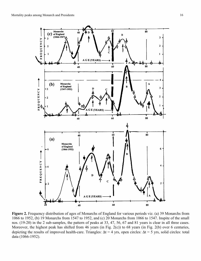
Figure 2. Frequency distribution of ages of Monarchs of England for various periods viz. (a) 39 Monarchs from

1066 to 1952, (b) 19 Monarchs from 1547 to 1952, and (c) 20 Monarchs from 1066 to 1547. Inspite of the small

nos. (19-20) in the 2 sub-samples, the pattern of peaks at 33, 47, 56, 67 and 81 years is clear in all three cases.

Moreover, the highest peak has shifted from 46 years (in Fig. 2(c)) to 68 years (in Fig. 2(b) over 6 centuries,

depicting the results of improved health-care. Triangles: Δt = 4 yrs, open circles: Δt = 5 yrs, solid circles: total

data (1066-1952).


genetically favored and fortunate enough to avoiddisease might live much longer than actuariallypredicted. Data fail to confirm the existence of suchevents. For example, adequate data on the numberof centenarians have been available in England since1837; over this time, despite a great change inaverage life expectancy, there has been no detectablechange in the number of people living longer than100 years or in the maximum age of persons dyingin a given year.”

Further amplification of this may be obtainedby examining two half sub-samples of the 2nd samplefor 1547 to 1952 A.D. viz. sample (d) from 1547-1702 and sample (e) from 1702-1952 A.D.Admittedly, these two sub-samples are small in nos.9 and 10, respectively, but the correspondingfrequency-distributions shown in Figs. 3a,b furtherbear out the above conclusions strikingly. Thus, wesee that:(i) the peak at 68 years in Fig. 3b has been

replaced in Fig.3a by 2 peaks: at 69 years and82 years, respectively; the latter clearlyreflecting the effects of better health-care;

(ii) the broad large inflected peak near 53 years inFig.3b has been replaced by two small peaksat 48 years and 57 years.

It would be seen later that the above-notedage-distribution of monarchs for 1702-1952 A.D.is in fact found to be nearly identical with the totaldistribution for the 36 U.S. Presidents from ~ 1750to 1994 A.D., which has 2 small additional peaksshowing up at 90 and 100 years (see Fig.4).

Table 2. Dates of birth and death of deceased Presidents ofU.S.A.


———————————————————George Washington 1732 1799 67John Adams 1735 1826 91Thomas Jefferson 1743 1825 83James Madison 1751 1836 85James Monroe 1758 1831 73Jhon Quincy Adams 1767 1848 81

Andrew Jackson 1767 1845 78Martin Van Buren 1782 1862 80William Henery Harrison 1773 1841 68Hohn Tylor 1790 1862 72James Knox Polk 1795 1849 54Zachary Taylor 1784 1850 66Milliard Filmore 1800 1874 74Franklin Pierce 1804 1869 65James Buchanan 1791 1868 77Abraham Lincoln 1809 1865 56Andrew Johnson 1808 1875 67Ylysses Simpton Grant 1822 1895 73

———————————————————Rutherford Birchard Hayes1822 1893 71James Abram Garfield 1831 1881 50Chester Alan Arthur 1829 1886 57Grover Cleveland 1837 1908 71Benjamin Harrison 1883 1901 68William McKinley 1843 1901 58 Theodore Roosevelt 1858 1919 61 William Howard Taft 1857 1960 103 Woodrow Wilson 1856 1924 68 Warren Gamaliel Harding 1865 1923 58 Calvin Coolidge 1872 1933 61 Herbern Clark Hoover 1874 1964 90 Franklin Delao Roosevelt 1882 1945 63 Harry S. Truman 1884 1972 88 Dwight David Eisenhower1890 1969 79 John Fitzgerald Kennedy 1917 1963 46 Lyndon Baines Jhonson 1908 1973 65 Richard Milhous Nixon 1913 1994 81———————————————————

Table 3. Data (birth and death) of the 9 Mughal kings of India.


———————————————————Zaheeruddin Babar 1483 1530 47Nasiruddin Humayoon 1508 1556 48Jalaluddin Akbar 1542 1605 63Noorulddin Jahangir 1569 1627 58Shahabuddin Shahjahan 1592 1667 75Muhayuddin Almgir 1618 1707 89Farukh Seyar 1663 1719 56Shah Alam 1727 1806 79Bahadur Shah Zafar 1775 1862 87

———————————————————For analysis, the data for any one Table were

arranged in ascending order of age at death, andthis was then sampled at 2 intervals viz. Δt = 4 yearsand t = 5 years, as in previous papers. This gave theresults shown in Tables 4a and b for the monarchsof England and in Tables 5a and b for US Presidents.In each of these Tables, analysis of the first half ofthe relevant data is presented in the first row, andthe second half is given in the second row, as indicatedin the right-hand columns of the corresponding row.


Figure 3. (a) & (b). Frequency distribution of ages two sub-samples of 9 & 10 Monarchs of England from (a)

1702 to 1952 and (b) 1547-1702, which further confirm the increasing height of the 67 years peak, plus the

appearance of the peak at 81 years in recent times. (c) the corresponding plot for ages of 9 Mughal Kings of India

(1500-1862), which shows a considerably different pattern of 5 peaks, with two pairs of large peaks (indicated by

vertical arrows); those at 48 and 57 are seen in case of the Monarchs of England. Fig. 3a & b: triangles for Δt = 4

yrs, open circles for Δt = 5 yrs, Fig 3 c: open triangles for Δt = 4 yrs, solid circles for Δt = 5 yrs.


Figure 4. The corresponding analysis for ages of the first 36 Presidents of the U.S.A. (d. 1799-1994). Fig. 4(a) shows the total plot

for all the 36 Presidents, depicting a main peak around 71 years, while Fig. 4(b) and 4(c) show respectively the corresponding plots

for the first 18 Presidents and the second 18 Presidents. Prominent peaks are to be seen in all three graphs around 47, 58, 70, and 81

years, indicated by the letters D, C, B & A, respectively. In addition, peaks are to be noted around 90 and 100 years in Figs. 4(b) and

(c), and also around 65 in Fig. 4(c). Triangles: Δt = 4 yrs, open circles: Δt = 5 yrs, solid circles: total data (1799-1994)


Table 4a: Monarchs of England [(1066-1547) and (1547-1952)], Δt = 5 years.

Table 4b. Monarchs of England, Δt = 4 years.

Table 4c. Two small sub-samples from monarchs of England (1547-1701 and 1702-1952). Top row with Δt = 5 years; bottomrow with Δt = 4 years.

Note: Top row with Δt = 5 years; bottom row with Δt = 4 years.

Table 5a. Ages of deceased Presidents of U.S.A. (1799-1890 and 1890-1994), Δt = 5 years.

Table 5b. Ages of deceased Presidents of USA (1799-1895 and 1896-1994), Δt = 4 years

Table 6. Ages of Mughal kings of India.

(a) Δt = 5 years

(b) Δt = 4 years

< 30 31-35, 36-40 41-45, 46-50 51-55, 56-60 61-65, 66-70 71-75, 76-80 81-85, 86-90 91-951 3 - 4 4 1 3 2 2 0 0 0 0 - (1066-1547)

� = 20 1 1 - 1 2 2 2 0 5 2 1 2 0 - (1647-1952)

� = 19 2 4 0 5 6 3 5 2 7 2 1 2 0 Total = 39

< 30 31-34, 35-38, 39-42, 43-46, 47-50 51-54, 55-58, 59-62, 63-66, 67-70 71-74, 75-78, 79-82, 83-86, 87-90 91-94, 95-98 1 2 1 2 3 3 1 2 1 2 2 0 0 0 0 0 - (1066-1547)

� = 20 1 1 0 1 0 2 1 2 1 0 5 2 1 2 0 0 - (1547-1952)

� = 19 2 3 1 3 3 5 2 4 2 2 7 2 1 2 0 0 - Total = 39

2 1 1 2 1 0 2 0 0 0 0 - � = 9 < 39 39-42, 43-46, 47-50 51-54, 55-58, 59-62, 63-66, 67-70 71-74, 75-78, 79-82, 83-86, 87-90 91-94, 95-98, 99-102

0 1 0 1 1 1 1 0 2 0 0 0 0 0 - � = 9

2 0 1 0 1 0 3 2 1 2 0 0 - � = 10 < 39 39-42, 43-46, 47-50 51-54, 55-58, 59-62, 63-66, 67-70 71-74, 75-78, 79-82, 83-86, 87-90 91-94, 95-98, 99-102

0 0 0 1 0 1 0 0 3 2 1 2 0 0 0 - � = 10

31-35, 36-40, 41-45, 46-50 51-55, 56-60, 61-65, 66-70 71-75, 76-80, 81-85, 86-90 91-95 0 0 2 0 2 1 0 1 1 0 2 0

41-45, 46-50 51-55, 56-60, 61-65, 66-70 71-75, 76-80, 81-85, 86-90 91-95, 96-100, 101-105 1779-1890 - 0 1 1 1 4 4 2 3 1 1 - � = 18

1890-1994 - 2 - 3 4 2 2 1 1 2 - - 1 � = 18

Total - 2 1 4 5 6 6 4 4 3 1 - 1 � = 36

39-42, 43-46, 47-50 51-54, 55-58, 59-62, 63-66, 67-70 71-74, 75-78, 79-82, 83-86, 87-90 91-94, 95-98, 99-102

1799-1895 - - - 1 1 - 2 3 4 2 2 1 1 1 - � = 18

1896-1994 - 1 1 - 3 2 2 2 2 - 2 - 2 - - 1 � = 18

Total - 1 1 1 4 2 4 5 6 2 4 1 3 1 - 1 � = 36

31-34, 35-38, 39-42, 43-46, 47-50 51-54, 55-85, 59-62, 63-66, 67-70 71-74, 75-78, 79-82, 83-86, 87-90

0 0 0 0 2 0 2 0 1 0 0 1 1 0 2


Figure 5. Mortality according to age, in the absence ofpremature death.

Analysis of age-distribution of the Presidents ofU.S.A. from 1750 to 1994.

Another good sample that is readily available isthat of the 36 Presidents of U.S.A. (d. 1799-1994).The dates of birth and death of these 36 are collectedin Table 2; two of these, namely Lincoln and Kennedy,are known to have been assassinated, but this couldperhaps be considered a risk of the profession! Ofcourse, the distribution is truncated below 40,because no one became President before this age.

The frequency analysis of the ages of these 36Presidents has been carried out in Tables 5a and b asbefore, breaking them down into two groups: (a) first18, who died between 1799 and 1894 ± 1, and (b)second 18 who died between 1894 ± 1 and 1994.The data is plotted in Figures 4a, b and c respectively,for: all 36, the first 18 and the second 18 presidents,respectively; the circles are for sampling interval Δt =5 years, the triangles for Δt = 4 years, with correctingfactor of 5/4 for the frequencies. These three plotsexhibit the expected peaks of mortality in theneighborhoods of 82 years, 66 –70 years, 58 years,and 48 years, with an additional small one at therelatively high age of 90 years, as also a trace of onearound 100 years! The curve does not go below 40years, because no one became a President beforethat age.

Also, it can be seen by comparison with Figs.2a-c for the monarchs of England that four of the peaks,namely those at 47, 58, 71 and 81, are within a yearor two of those (47 ± 1, 57 ± 1, 68 ± 1 and 81)found in case of the monarchs. Closer examination ofthe 3 distributions of Figs. 4a-c shows that the relativelysmall peaks at 48 years and 100 years are to be seenonly in the distribution for the 2nd 18 Presidents.While the peak at 100 years can be attributed toimproved health and health-care services, that at 48years is linked with assassination and stroke, both ofwhich could justifiably be considered today as a

politician’s risk! The 2nd plot for the U.S.Presidents (from 1890 to 1994) also shows thepossible appearance of another peak, around 62years of age, which needs further exploration.

Discussion and comparison with mortalitypeaks for Mughal kings

The above comparison provides grounds forthe conclusion that the main peaks of mortalityobserved at or near 47, 57, 68 and 81 years are adefinite feature of the life-spans in these countries,at least amongst people of Anglo-Saxon ancestry.We may note here that, as noted by Comfort [12]and Upton [13] in 1990, the survival curve in theUnited States was not very different from thissituation. However, sequential survival curvesthroughout this century show progressive“rectangularization as the elimination of prematuredeath results in a sharp down-slope to the naturallife span (Fig.5). The serial data allow calculationof the position and shape of a survival curve if allpremature deaths were eliminated: an ideally“rectangular” survival curve. If we assume a normalbiologic distribution, statistics suggest that underideal societal conditions mean age at death is notfar from 85 years.


The data on monarchs of England and Presidentsof U.S. not only bear out the above generalizedstatement, but in addition shows that the pattern ofmortality in any one set of samples is in factcomposed of distinct peaks, the main ones being ator around the ages of 47 ± 1, 58 ± 1, 69 ± 2, 81 ±1, together with a smaller one around 91 and around33 years. These four main peaks of mortality (labeledD to A respectively in the diagrams) are thus typicalof the pattern of aging, at least in these two countries.As indicated in an earlier paper, the first two aremostly associated with various killer diseases e.g.cerebral hemorrhage and coronary or other stroke,while the two highest represent mostly the effects ofgeneral physical degeneration of the body organs.

From the curves of Figs. 2, 3 and 4, it is alsoseen that the result of better nutrition and health-care over the last few centuries has been to shift themaximum mortality towards the higher peaks. Forexample, in Fig.3b (1647-1702) and Fig.3a (1702-1952), 45% ± 5% of the total mortality among U.K.monarchs is seen to correspond to the largest peak,which has shifted from ~ 46 years to 68 years overa period of 2 centuries. This shift is apparentlycontinuing a little further, as seen from Figs. 3b andc for U.S. Presidents (1786-1890) and (1890-1995). In fact, a small peak at 102 years is nowapparent in Fig. 3c, corresponding to the latestsituation in the 20th century, but this is compensatedby another one coming up at 62 years in Fig. 4c (forthe period 1890-1995), which needs further study.

J. Fries [1] states: “By implication, the practicalfocus on health improvement over the next decadesmust be on chronic instead of acute disease, onmorbidity not mortality, on quality of life ratherthan its duration, and on postponement rather thancure----. An important shift is occurring in theconceptualization of chronic disease and of aging.Premature organ dysfunction, whether of muscle,heart, lung, or joint, is beginning to be conceived asstemming from disuse of the faculty, not overuse.”

Finally we show, in Fig. 2c, a plot of the ages of9 Mughal kings of India (1500-1900 A.D.), whichshows a pattern that involves two pairs of large peaksat 48, 57, 77 ± 2 and 88 years. The peak at ~ 79years is to be seen in the corresponding patterns ofMortality peaks of British monarchs (1542-1995)and also the U.S. Presidents, but the others do notfully fit either of these patterns at all.

So, there appears to be a need to make furthercomparative studies of this type, using appropriatesamples taken from various regions and races of theworld, in order to elaborate some of the points notedabove.

References

1. Fries, J.F. 1980. Aging, natural death compressionof morbidity. New Eng. J. Med. July 17.

2. Qurashi, M.M. and Shah, M.A. 1984. Scientometricstudies on Muslim scientists, Part II. Proc. PakistanAcad. Sci. 21:25-36.

3. Qurashi, M.M. 1993. Scientometric Studies onMuslim Scientists of Pakistan (d. 1970-1992. S.T.I.W.11:75-88.

4. Qurashi, M.M. and Khan, S.A. 2000. Periodicity ofAge Distribution. Proc. Pakistan Acad. Sci. 37:211-222.

5. Siddiqi, A.F. 2000. Human Age Distribution: A SampleSurvey. Science Vision 6:21-24.

6. Qurashi, M.M. and Kazi, A.Q. 2003. A PreliminarySemi-Clinical Study. Pak. J. Med. Res. 42:191-199.

7. http://www.britannia.com/history/h6f.html8. h t t p : / / e n . w i k i p e d i a . o r g / w i k i /

List_of_British_monarchs9. http://soundnumbers.com/36html10. http://www.americanpresidents.org/presidents/

gwashington.asp11. Urdu Dyra Mostofa-Islamia, Lahore, vol.21, p. 392,

1987.12. Comfort, A. 1979. The Biology of Senescence. 34th

ed., New York, Elsevier Press, pp. 81-86.13. Upton, A.C. 1977. Pathology. In: Handbook of the

Biology of Aging. Eds. Finch, L.E. and Hayslick L.,

pp. 513-35. New York, Van Nostrand Reinhold.


procedings of pakistan academy of sciencespaspk.org/wp-content/uploads/proceedings/42 no. 1... ·...

Documents