procedural terrain generation using a level of detail ... · procedural terrain generation using a...
TRANSCRIPT

Procedural Terrain Generation using a Level of Detail System
and Stereoscopic Visualization
Octavian Mihai Vasilovici
Master of Science, Computer Animation and Visual Effects
August 2013
Bournemouth University

Abstract
Terrain generation using height maps is still largely used due to its benefits of offering great
control and being a straightforward method. It can be used in either real-time rendering or not. For
real time rendering however, sometimes it becomes problematic when trying to directly renderer a
highly detailed mesh as the polygon number is very big.
This paper is focused around implementing the one of the latest published method of terrain
generation for real-time rendering, namely, Continuous Distance-Dependent Level of Detail. Besides
the implementation of the algorithm it also employs stereoscopic rendering and the Instance Cloud
Reduction algorithm for visualization purposes, while trying to simulate a real case rendering
scenario that is found in modern games. The implementation is done using C++, NGL and OpenGL
4.0 core profile.
The current paper, does not try to improve any of the algorithms presented, but instead it tries
to provide a clean implementation and modular integration of the described methods.

Table of Contents
Abstract ................................................................................................................................................................. i
1. Introduction and Motivation ........................................................................................................................... 1
2. Previous Work .................................................................................................................................................. 1
3. Technical Background ...................................................................................................................................... 2
3.1 Chunked LOD .............................................................................................................................................. 2
3.2 Continuous Distance-Dependent LOD ........................................................................................................ 3
3.2.1. LOD Distances and Morph Areas ........................................................................................................ 4
3.2.2. Quadtree Traversal and Selection ...................................................................................................... 5
3.3 Stereoscopic Visualization .......................................................................................................................... 7
3.4 Instanced Cloud Reduction ....................................................................................................................... 11
3.4.1. Culling Pass ....................................................................................................................................... 12
3.4.2. Rendering Pass ................................................................................................................................. 12
4. Implementation ............................................................................................................................................. 14
4.1 CDLOD Implementation ............................................................................................................................ 15
4.1.1. Terrain Class ..................................................................................................................................... 16
4.2 Stereoscopic Rendering Implementation ................................................................................................. 17
4.3 Instance Cloud Reduction Implementation .............................................................................................. 19
4.4 User Interface Implementation ................................................................................................................ 19
5. Results and Analysis ...................................................................................................................................... 20
5.1 CDLOD Algorithm ..................................................................................................................................... 20
5.1.1. Mesh Generation. No LOD System ................................................................................................... 20
5.1.2. Mesh Generation. CDLOD System .................................................................................................... 21
5.1.3. LOD Selection Based on Height ........................................................................................................ 22
5.1.4. LOD Selection using Bounding Boxes ............................................................................................... 22
5.1.5. Morphing between LOD levels ......................................................................................................... 23
5.2 Stereoscopic Visualization ........................................................................................................................ 24
5.3 Performance Results ................................................................................................................................. 25
5.3.1. GPU Performance ............................................................................................................................. 25
5.1.2. CPU Performance ............................................................................................................................. 25
5.1.3. Memory Allocation Performance ..................................................................................................... 26
6. Conclusions and Future Work ....................................................................................................................... 27
7. References ..................................................................................................................................................... 28
Annex A ............................................................................................................................................................. 29

1
1. Introduction and Motivation
Terrain generation and rendering them real-time is a frequent requirement in various applications such
as games and graphics engines. Terrain generation from heightmaps is still very largely used due to its
simplicity and good control over the generated terrain that it offers.
The simplest way to generate and render a terrain from a heightmap is by using the brute force
approach, in which every vertex from the mesh corresponds with a pixel read from the read texture. For very
large datasets this is not practically possible without sacrificing a lot of performance and thus a Level Of
Detail (LOD) algorithm it is needed. In short, a LOD system is responsible with decreasing or increasing the
complexity of a 3D object representation based on the distance towards the viewer or any other metric
employed in the graphics engine.
Terrain generation and rendering is vastly used in computer games where performance is crucial.
Besides the terrain, other object are rendered and other techniques are used, like post processing effects,
ambient occlusion, antialiasing, etc and thus limiting the performance of the engine even more.
While the current paper is focused on terrain generation and rendering using a Continuous Distance-
Dependent Level of Detail algorithm, a couple of other methods were used to better reflect the performance
and importance of using a Level Of Detail scheme in a real scenario: instanced rendering of 3D objects using
geometry shader culling and stereoscopic rendering.
2. Previous Work
Over the years, many LOD algorithms were developed for handling terrain rendering. The early
algorithms were executed on the CPU, like the academic algorithm introduced by Duchainea et al. in 1997.
However, starting with the GPU increase in raw power, the benefit of shifting these algorithms on the GPU
became evident.
According to Strugar P.(2010), in the current context of modern PCs and game consoles there is little
to no benefit having a terrain algorithm to produce an optimal triangle distribution by using the CPU if it
cannot provide enough triangles for the graphics pipeline, or if it uses too much CPU processing power.
According to Wloka M., (2004) the graphics API, driver and the operating system between the CPU and GPU
is also a common bottleneck and thus even a simplistic GPU-based algorithm can be faster and provide better
visual results than a complex one that is executed on the CPU.
One of the first algorithms to be fully GPU-oriented was developed by Ulrich T. in 2002. The
Chunked LOD algorithm is still vastly used due to its ability to get a good detail distribution and an optimally
tessellated mesh. The technique generates static meshes in a preprocessing step which are then stored at
different LOD levels in a quadtree. At runtime, the needed LOD is computed, extracted and rendered from the
quadtree. When a quadtree with different LOD levels is met, cracks will appear in the mesh. In order to avoid

2
this, Ulrich T., (2002) proposes a hybrid solution by using simple triangles that extend vertically at the edge of
the patch to cover the cracks that appear.
In 2010, Strugar F., introduced the Continuous Distance-Dependent Level of Detail algorithm that
starts from the premises of the algorithm developed by Ulrich T.(2002) and features a fixed grid mesh where
the height information is directly read from the heightmap and the mesh is displaced in the vertex shader. It
uses a quadtree structure and a predictable continuous LOD system.
The selection algorithm assures the on-screen triangle distribution is kept constant and is not
influenced by the distance to the viewer.
3. Technical background
3.1 Chunked LOD
Since the CDLOD algorithm presented by Strugar F., (2010) builds upon the Chunk LOD algorithm
developed by Ulrich T., (2002), an overview of this algorithm is needed. The algorithm uses a quadtree to
store the different LOD levels. At runtime the LOD levels are selected from the quadtree and rendered. If
quadtree nodes with different LOD levels are met, cracks will appear around the borders. In order to fix this,
Ulrich T., proposed to use simple triangles that extend vertically at the edge of the patches to cover these
cracks. This means that the bottom edge of a triangle needs to extend below the full LOD of the mesh at the
edge of the patch and has to extend below any possible simplification of the maximum LOD.(Cervin A.,
2012)
The rendering of the terrain chunks (nodes) is done based on the distance to the viewer(camera). This
means that for a certain view, chunks are selected from the quadtree in order to match the fidelity of the
terrain mesh. Each chunk has a maximum geometric error associated and bounding box volume. The
calculation of each node to be use,d is done by the following formulae:
� =�
��
(3.1)
� - maximum screen space error that a selected node(chunk) will result in
� - maximum geometric error associated with the node
D - distance from the camera to the closest point of the node.
K - is a perspective scaling factor that takes into account the size of the viewport and field of view.
� = ���� �����ℎ
2����� ����������
2
(3.2)

3
The rendering of a node it is done by traversing the quadtree from the root using a predefined
maximum tolerable screen space error. If the current node is acceptable by calculating the maximum screen
error using (1.1) formulae then it is rendered. Otherwise, if the current node's error is too large, the traversal
continues with the children of the node.
In order to avoid the "popping-in" visual effects that normally appear when a parent node is selected
with a child node for rendering, a small morph is being used for each vertex on the vertical coordinate. The
morph parameter is the same for the whole node. The morph parameter can have two possible values: 0 if the
node is about to split and 1 if the node is about to merge. This behavior determines the consistency over LOD
switching.
The morph parameter can be calculated with the help of (1.1) equation:
������ = ��!�(2�
#− 1,0,1)
(3.3)
������ = 0 at the distance where a node is split into 4 smaller ones.
������ = 1 at the distance where 4 nodes will merge into 1 node.
The equation is based around the fact that � of a parent node equals 2� for the child nodes.
3.2 Continuous Distant-Dependent LOD
The CDLOD algorithm developed by Strugar F., (2010) expands upon the CLOD algorithm by using
a continuous morph between LOD levels. It also fixes some of the existing problems in the CLOD algorithm
and the mimaps algorithm by Asirvatham A., presented in GPU Gems 2 (2005).
One major problem of the mipmaps algorithm is that the LOD is basically based on two-dimensional
components (latitude and longitude) of the viewer position while ignoring the height. According to Strugar F.,
(2010) this results in an unequal distribution of mesh complexity and aliasing problems when the observer is
at a higher position above the terrain mesh while the detail level still remains higher than actually needed.
The CLOD algorithm developed by Ulrich T., (2002) improves upon the limitations of the mipmaps
method, by using a LOD function that provides an approximation of the three-dimensional distance-based
LOD which is the same over the whole node. The obvious drawback of this method can be easily seen in
normal scenarios encountered in modern games where the terrain is very uneven and the position and height
of the viewer changes quickly thus resulting in poor detail distribution or movement-induced rendering
artifacts. It can also have integration difficulties with other rendering systems since the unpredictable LOD
system can cause rendering errors such as mesh intersection or floating of other 3D objects placed on the
terrain. (Strugar F., 2010)
The CDLOD algorithm solves all these issues by employing a fully predictable LOD distribution
which uses a direct function of three-dimensional distance across all rendered vertices. In contrast to the

4
hybrid method used by the CLOD algorithm for filling cracks, the CDLOD one does not require the use of
any additional geometry for stitching. Instead, the higher level terrain mesh is fully transformed into the
lower version before any switching occurs. Another benefit of this method is that also no "popping" appears
when transitioning from one LOD level to the other.
3.2.1 LOD Distances and Morph Areas
The first step of the rendering is the selection of the nodes from the quadtree. This selection is
performed every time the viewer(camera) moves. The quadtree depth always corresponds with the level of
detail. This constraint is introduced in order to allow the same grid mesh to be used in rendering every
quadtree node while maintaining a fixed triangle count.
Based on the above, a child node will always have 4 times more mesh complexity per square area than
its parent since a child node will occupy a forth of the area. Thus, each successive LOD level will render 4
times as many triangles and contains 4 time more nodes than its parent. (Strugar F., 2010)
Fig. 3.1 Quadtree and LOD layers - Strugar F., 2010
In order to know what node to be selected in each region, distances that cover each LOD level need to
be pre-calculated before the selection is done. These distances are then saved in an array of LOD ranges.
Based on the fact that the complexity difference between each successive LOD level is four as per the
algorithm design, the difference in the distance covered by them needs to be close to 2.0 in order to
accomplish a relatively even triangle distribution.
Fig. 3.2 Distribution of six LOD ranges - Strugar F., 2010

5
The smooth LOD transition is done by defining a morph area in order to mark the range along which
the higher complexity mesh will change into a lower one. According to Strugar F., (2010) these areas cover
around 15%-30% at the end of each LOD level.
3.2.2 Quadtree Traversal and Node Selection
After the array containing the LOD distance is created, it is used in the selection of nodes representing
the currently observable part of the terrain. The quadtree is recursively starting from the most distant nodes (
less detailed mesh ) going down to the nearest (most detailed mesh) ones. This selection is later used for
rendering the terrain. (Strugar F., 2010)
The pseudo code for the algorithm presented by can be described as:
bool Node::LODSelect( ranges[], lodLevel, frustum )
{
if not node_Bounding_Box_Intersects_Sphere( ranges[ lodLevel ] ))
return false;
if( lodLevel == 0 )
Add_Whole_Node_To_Selection_List( );
return true; // we have handled the area of our node
else if not node_Bounding_Box_Intersects_Sphere( ranges[lodLevel-1])
Add_Whole_Node_To_Selection_List( ) ;
else
foreach( childNode )
if not child_Node.LODSelect( ranges, lodLevel-1, frustum )
Add_Part_Of_Node_To_Selection_List( childNode.ParentSubArea )
return true; // we have handled the area of our node
}
Since the LOD level selection uses the actual three-dimensional distance from the viewer, it works correctly
for every terrain configuration and any viewer heights.

6
Fig. 3.3 LOD Selection at different heights - Strugar F., 2010
The rendering of the terrain is done by iterating through all the selected nodes. The continuous
transition is done by morphing the area of each level into a less complex one to achieve a seamless transition
between them. (Strugar F., 2010)
Unlike the CLOD algorithm were the morphing is done per chunk in the CDLOD algorithm the
morphing is done per vertex. Each nodes supports a transition between two LOD levels: its own and the next
and previous ones. The morphing is thus, done in the vertex shader. The distance between the viewer and a
vertex must be calculated in order to determine the amount of morphing that is needed. This step is necessary
in order to avoid the seams as the vertices on the node's edges must remain exactly the same as the ones on
the neighboring nodes. Strugar F., (2010) defines a morph vertex as being a grid vertex that has one or both
of its grid indices (i, j) as an odd number, and its corresponding no-morph neighbor as having the coordinates
(i – i/2, j – j/2). The morph operation will change every block of eight triangles from the more detailed mesh
in a block of two triangles corresponding with the less detailed mesh by gradual enlarging two triangles and
reducing the remaining six triangles into degenerate triangles that will not be rasterized. This process
produces smooth transitions with no seams or T-junctions as it can be seen in the following image:
Fig. 3.4 Grid Mesh Morph Steps - Strugar F., 2010

7
3.3 Stereoscopic Visualization
Many methods and hardware for visualizing stereoscopic context exists today. However, the
principles of rendering in stereo 3D are the same. In contrast to plain 3D (monoscopic) rendering, in a stereo
context the same scene needs to be rendered two times: one time for the left eye and one time for the right
eye.( Mishra A., 2011) In stereoscopic visualization another parameters from optics is introduced: parallax.
According to Mishra A., (2011) the human visual system requires depth cues from a flat image in
terms of how much a specific object shifts laterally between the left and the right eye. The parallax is defined
as this kind of displacement. Thus, the parallax is a numeric value which can be calculated and it's values can
be positive, zero and negative. In practice the parallax is created by defining two cameras for the left and right
eye separated by a distance, called interocular distance or eye-separation and by having a plane at a certain
distance along the viewing direction at which the parallax is zero. Objects that exists at a parallax plane of
zero will be at the same depth as the screen (screen-depth). Object closer to the camera will seem to be out of
the screen (pop effect) while objects farther than the plane of zero parallax will be inside the screen (push
effect).
Fig. 3.5 Parallax resulting at different depths - Mishra A., 2011
While not being crucial when implementing stereoscopic rendering, calculating the parallax can have
substantial importance in the planning of the stage phase and overall range of usable parallax in the
application.

8
According to Mishra A., (2011), parallax can be calculated as follows by using the intercept theorem:
a) Vertex beyond convergence point b) Vertex closer than convergence point
Fig. 3.6 Parallax resulting at different depths - Mishra A., 2011
a) for a vertex that is located at ) depth and beyond the convergence distance:
*+
,-=
�+
�-
(3.3.1)
By the similarity of ∆+�/ ~ ∆�-1
�+
�-=
�/
-1=
) − 2
)= 1 − 2/)
(3.3.2)
Thus,
*+
,-=
�
�= 1 −
2
)<=> � = �(1 −
2
))
(3.3.3)

9
b) for a vertex that is closer than the convergence distance:
*+
,-=
+�
�-=
+�
+- − +�=
+�+-
1 −+�+-
(3.3.4)
Since �/ ||-1 :
+�
+-=
�/
-1=
2 − )
2= 1 − )/2
(3.3.5)
Thus,
*+
,-=
�
�=
1 − )/2
)/2=
2
)− 1 <=> � = −�(1 −
2
))
(3.3.6)
The negative sign in the above equation implies that the vertex projections a that are on the
convergence plane are on opposite sides as the corresponding cameras. (Mishra A., 2011)
Thus, the variation of the parallax with the depth of the vertex for a specific convergence distance and eye-
separation can be drawn as follows:
Fig. 3.7 Parallax budget of a vertex based on convergence and separation - Mishra A., 2011
As discussed above, for stereoscopic rendering a twin-camera setup needs to be set. A representation of such
a setup can be viewer in the following image:

10
Fig. 3.8 Parallel asymmetric frustum - Mishra A., 2011
In the above image we have two view frustums:
- one originating at L (left eye)
- one originating at R (right eye)
- the distance LR is the eye separation, so the offset from the origin for each eye is 78
9
As it can seen in the above picture there are 2 asymmetric frustums. This is done in order to fix the vertical
parallax which can occur if a "Toe-in" method is being used. (Bourke P., 1999) In the above image we can
clearly see that each frustum is parallel to the other and thus the name "Asymmetric frustum parallel
projection".
The frustum for each eye can be calculated as follows:

11
Fig. 3.9 Projection Matrix calculation in OpenGL - MSDN
��� = �:;<����=���>
2
(3.3.7)
?����! = −���
(3.3.8)
The half-width of the virtual screen is:
� = <@�;AB2���=���>
2
(3.3.9)
Looking at the left frustum ALB , the near clipping plane intersects it at �C;DB distance of LL' and ��EF�B
distance right of LL'
�C;DB
?=
��EF�B
=
�:;<�
2
(3.3.10)
? = � −�;G;
2
(3.3.11)
= � +�;G;
2
(3.3.12)
Calculating �C;DB and ��EF�B for the right frustum is done by swapping b and c in the above equation.
3.4 Instance Cloud Reduction
In order to better show the stereoscopic 3D visualization effect, extra geometry was added to the
terrain mesh. The approach used was developed by Rakos D., 2010.
The rendering process involves two steps:
- A culling pass performed in the geometry shader.
- A rendering pass using instanced rendering.

12
3.4.1 Culling Pass
The first pass will be provided with the information about the instances on which the frustum culling
will be performed. This information will be fed by using two inputs:
- Instance transformation data
- Object extents information containing the instance position and an extend based on which a bonding box
volume will be created and culling performed. (Rakos D., 2010)
The culling pass shader consists of a vertex and geometry shader. The vertex shader determines if the
actual object is inside the view frustum or not and sends a flag to the geometry shader. The geometry shader
will then emit the instance data to the destination buffer if the object is visible or will not emit anything if the
object is outside the viewing volume.
In order to capture the primitives emitted by the geometry shader a transform feedback is being used.
The capturing is stored in another buffer object that will be used in the actual rendering pass.
The pipeline of the culling pass can be observed in the following image:
Fig. 3.10 Culling Pass Pipeline Diagram - Rakos D., 2010
3.4.2 Rendering Pass
In the second pass the data buffer used for storing the primitives from the culling pass must be
sourced by reading the asynchronous query results from the first pass.
The whole pipeline for the technique can be seen in the following image:

Fig. 3.11 Rendering
This technique has numerous advantages over other methods including
- Reduced amount of processed data
- No need for any space partitioning methods since the culling is done dynamic
- Can handle large amount of instanced objects
- Scales well with an increased number of instances
The obvious disadvantage is that it requires an extra pass for culling and it uses asynchronous queries
to determine the number of visible instances
endering Pipeline Diagram - Rakos D., 2010
This technique has numerous advantages over other methods including:
No need for any space partitioning methods since the culling is done dynamic
instanced objects
Scales well with an increased number of instances
The obvious disadvantage is that it requires an extra pass for culling and it uses asynchronous queries
to determine the number of visible instances. (Rakos D., 2010)
13
The obvious disadvantage is that it requires an extra pass for culling and it uses asynchronous queries
14
4. Implementation
The implementation of the algorithms was done in OpenGL using C++, the NGL lib for 3D
mathematical manipulation and Qt for the user interface. Since the project is rather big in scope a careful
consideration went towards the application design. Hardware and driver limitations also provided a strong
influence in the final design of the application. The aim was to provide an application that is flexible, easy to
use, has all the needed parameters exposed without requiring the source code to be compiled each time, is
modular and coherent in design, is fully UI driven and the visualization can be done either in a monoscopic or
stereoscopic context based on the hardware that it runs on. The application emphasis on correct stereoscopic
rendering, correct implementation and usage of the CDLOD terrain generation algorithm. The instanced
rendering of vegetation objects was employed only to better reflect the stereoscopic effect and to better see the
depth of the rendered scene. It also proves one of the key aspects of the CDLOD algorithm, that of easier
integration with other algorithms.
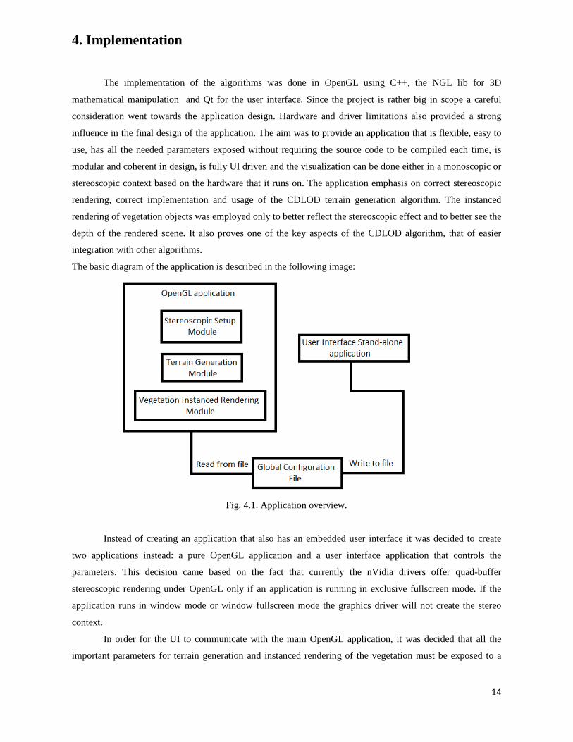
The basic diagram of the application is described in the following image:
Fig. 4.1. Application overview.
Instead of creating an application that also has an embedded user interface it was decided to create
two applications instead: a pure OpenGL application and a user interface application that controls the
parameters. This decision came based on the fact that currently the nVidia drivers offer quad-buffer
stereoscopic rendering under OpenGL only if an application is running in exclusive fullscreen mode. If the
application runs in window mode or window fullscreen mode the graphics driver will not create the stereo
context.
In order for the UI to communicate with the main OpenGL application, it was decided that all the
important parameters for terrain generation and instanced rendering of the vegetation must be exposed to a

15
single configuration file that can be accessed by both applications. A full class diagram can be seen in
Appendix A.
In the above diagram it can be easily seen that each of the methods resides in its own contained
module and thus, each module can be enable or disabled if needed: The stereoscopic setup module can be
easily swapped with a monoscopic one, the vegetation instanced rendering module can be disabled or
swapped with any other geometry rendering module, etc.
4.1 CDLOD Algorithm Implementation
The implementation follows the rules described in the third chapter and is based on the translation of
the DirectX source code Strugar P.(2010). It also features some of the optimizations presented in the original
paper. Since the desire was to be able to push the algorithm and LOD system to the maximum some decisions
were made.
One of the first decisions was the selection of the type of variable that will hold the grid information.
Initially, a vector was selected. Based on the paper published by Strugar P.(2010), the grid latitude is stored
in the X component, the longitude is stored in the Y component and the height in the Z component of a vector
of 3 elements. Thus a vector of a vector of 3 component was needed. Since a grid can be seen as a matrix of n
x n elements it quickly became obvious that a vector of vector of a 3 component vector was required in order
to keep all that information. But. instead of creating a vector of a vector, it was decided to use an offset in the
vector in order to store all the rows and columns of the grid in a single vector. In an attempt to further
optimize the performance the vector was swapped with a dynamic array, although based on testing, the
performance is almost the same and probably this doesn't provide any benefit due to the extra care needed for
handling the release of the allocated memory.
The generation and creation of the base terrain mesh using triangle strips is based around the same
technique described by Strugar P.(2010) in the source code accompanying his paper.
To keep the modular aspect of the application, all the grid generation methods were encapsulated in a
couple of classes using the template specialization techniques described by Macey J. 2012. These classes also
provides the mechanisms needed for selection a subset of the array used in the node selection algorithm
presented in chapter 3.
One of the improvements of memory costs described by Strugar P.(2010) is to keep only the
maximum and minimum height values a bounding box can have, rather than all corner points that create that
bounding box. For visualization purposes, another class was created that extends upon the bounding box class
in order to be able to visualize these bounding boxes used for selection. However, for the algorithm to work
properly this class is not needed.

16
The heightmap texture information that will be fed to the vertex shader was decided to be stored in a
simple class, using a vector for the height information and other variables and methods that are required for
OpenGL integration.
4.1.1 Terrain Class
This class is the core of the terrain generation and rendering algorithm. It contains all the methods
needed for generating the terrain mesh, creating the quadtree, selecting a node from the quadtree, rendering
the selected nodes and calculating the viewer distance used in the nodes selection. It features two main
methods, the initialization method and rendering method.
The initialization method is run only one time, at the start of the application. It is responsible for
reading all the parameters from the configuration file and the heightmap. The reading of the heightmap texture
is done by the QImage class and it handles both greyscale and color textures. In case of color textures the
height information is assumed to exist on the red channel of the texture. The height information is stored in a
bidimensional array of a maximum capacity of 4096x4096. This limitation is imposed in order to avoid
memory allocation problems. Initially, the decision was to re-size the heightmap to the actual size of the
generated grid. However, based on tests, it was discovered that QImage is unable to resize only to scale a
picture and thus, in order to get a correct representation of the height information, currently the texture file
must be manually re-sized at the same size as the grid used in the terrain generation.
Once the parameters are read from the configuration file, the actual terrain mesh is being generated by
using the information from the heightmap. This implementation is based around the algorithm of CLOD
described by Ulrich, 2002 as an pre-step before the application starts. The normals are also calculated in this
step based on the tangent and binormal vectors.
Afterwards, the mesh is partitioned and the quadtree is created based on the generated bounding boxes
following the algorithm described in chapter 3.
The number and size of the bounding boxes is created based on the node size that is provided in the
configuration file and thus the accuracy of the LOD selection can be fully controlled.
Next, the texture units are created for the rendering step, including the color textures and the
heightmap texture used in the shaders. Since procedural terrain texturing is another topic in itself, for
visualization purposes the "splatting" method of texturing was selected. In short this methods consist of a
texture that uses each color channel as an alpha channel in the selection of the texture images to be utilized.
This method is still highly used since it gives artist big freedom and is easier to use and implement.
The rendering method is used per frame and is responsible for calculating the distance from the
camera to the nearest point of a bounding box. Based on this distance a specific LOD level is selected. The
selectLodDraw() method is where the heart of the recursive selection algorithm described in chapter 3 is

17
implemented and the implementation is straightforward. Once a LOD level has been selected the actual
rendering is done by the drawPatch() method. This method consists of loading all the parameters to the shader
and rending the selected node as a series of triangle strips. The drawPatch() method is called for each node
that is selected for a specific LOD level and is also responsible for drawing the bounding boxes used for
visualizing the LOD selection.
Another method to mention is MoveOnTerrain(). This method tried to keep the camera position at a
specified height above the terrain to simulate terrain collision. This is done by extracting the position of the
viewer from the inverse of the view matrix as it is done in the rendering method when the distance from the
camera and a bounding box is calculated.
The current implementation features a configurable number of LOD levels and a fixed LOD level that
will always contain the high resolution mesh. The mesh is being generated as a series of triangle strips based
on the grid size provided by the configuration file. In order to be able to control the scale of the terrain mesh
and keeping the same triangle distribution, the grid scale parameter was introduced. The resulted terrain mesh
size in units is a direct result of the grid size multiplied by the scale. The obvious advantage of this is the
ability to generate a big scale mesh with a relative low number of triangles. To give even more control to the
type of generated terrain, the height of the generated mesh can also be directly controlled and thus providing
different results using the same heightmap information. Additionally, for each LOD level the distance where
the next LOD level is selected (the LOD brake) can be configured and is also exposed in the configuration
file.
The morphing of the vertexes is done in the GLSL vertex shader. The position of the current vertex is
calculated based on the VertexID and InstanceID from the instanced rendering. The morphing factor is
calculated as series of binary operations and can be further tweaked from the vertex shader.
Various other methods are used to facilitate the visualization of the LOD levels including coloring
each LOD level separately, displaying the bounding boxes used in the LOD selection, toggling wireframe in
order to see the triangle distribution across the landscape and different shading techniques.
The current implementation does not feature any type of frustum culling. This decision was done on
purpose in order to see the real impact on performance using this method. Implementing a frustum culling
technique is trivial and can be done by checking each bounding box used on LOD selection against the
frustum volume and not sending to the rendering pipeline those nodes that fail.
4.2 Stereoscopic Rendering Implementation
The stereoscopic rendering was developed as a stand-alone module. The StereoCamera() class is
based on the ngl::Camera() and expands on it in order to facilitate the stereoscopic needs. It is built around the
"parallel axis asymmetric frustum" algorithm described in chapter 3. It consists of methods for setting the left
and right camera perspectives and camera positions and other methods to ensure a coherent camera

18
manipulation. Some of the methods inherited from the ngl::Camera() class were overridden in order to create a
movable camera. It was decided that instead of moving the virtual world and keep the camera to a fix position,
to keep the world at a fixed position and move the camera location around the world as described in the
original algorithm by Strugar P.(2010). The StereoCamera() class does not employ any type of advanced
camera system, that would be normal in this scenario, like an orbit camera. For simplicity, it provides the
necessary methods to move the position and the look-at point around and it performs the yaw, pitch, roll and
slide functions.
One problem that quickly became evident was the fact that in the current implementation no central
pivot exists and thus, when a rotation bigger than 90 degrees around the camera up axis exists, the left and
right eye can become inversed. In order to overcome this problem a third monoscopic camera was created to
act as a central pivot for the stereo one. The scene is never rendered through this camera, but instead all the
camera manipulation functions are performed on it, after which the position, look and up vector are read and
the left and right eye perspectives and positions are updated.
Based on the SIGGRAPH presentation provided by Gateau S., et al (2010) and the algorithm
described in chapter 3, the following parameters play an important role in setting and manipulating the
stereoscopic visualization:
- Separation = interocular distance /screen width
- Convergence = distance to the zero parallax plane.
These two parameters are exposed to the user and can be changed from the application user interface.
The OpenGL implementation consists of:
- Create a stereo context
- Query the OpenGL API to see if such a context is supported by the platform.
- If yes, stereoscopic rendering is supported and the rendering is done using the QuadBuffering technique.
- If not, rendering is done in plain 3D, using the DoubleBuffering technique.
The QuadBuffering technique consists of a set of back and front buffer for the left and right eye.
Thus, the scene is rendered two times: one time in the left eye, and one time in the right eye. The left and right
eye are automatically swapped by the OpenGL API when a frame is rendered. By rendering the same scene
two times, theoretically the performance hit would be 50%. However, in practice this is not always true, since
in order to keep the screen and active shutter glasses synchronized, the vertical synchronization (VSync) is
automatically enabled by the driver in order for the application not to render more frames than the display can
actually show.
Since not every platform is capable of rendering in a stereo context and to ensure compatibility, a
monoscopic rendering method was also created and the scene is rendered from the left eye perspective only.

19
4.3. Instance Cloud Reduction Implementation
In order to better reflect the effect of stereoscopic rendering and depth perception it was decided that
additional geometry should be rendered on the landscape.
The implementation of the method is the same as the one described in chapter 3. The method was
created and integrated in its own module. It consist of an initialization phase, in which the same heightmap
texture is being read in order to get the height information, creating the geometry instances by using the height
information and randomly placing the geometry on the terrain using as maximum coordinates the same grid
size used in terrain generation.
The rendering phase is a two steps process. In the first step the, culling shader is being used to
determine which geometry is visible and in the second step it is rendered. The number of geometry instances
is exposed to the user via the configuration file. This technique does not employ any type of LOD mechanism
of rendering the instances meaning all the visible geometry will have the same number of polygons. The
reason behind this approach, was to simulate the polygon complexity and performance impact that would exist
in a real case scenario. The rendering of the instanced geometry can be disabled, at runtime, from the
application interface in order to reflect the performance difference.
4.4. User Interface Implementation
The application offers an on-screen user interface to enable different options in order to display how
the CDLOD algorithm is working and to control the stereoscopic rendering. Since stereoscopic rendering is
bound by the hardware and the nVidia drivers currently support QuadBuffered rendering using 3D Vision on
consumer graphics cards, only under Windows, when the application is set in exclusive fullscreen, it was
decided that the main application will not have any graphical user interface. Instead, a setup wizard was
created that controls all the parameters of the terrain generation and from which the user is able to launch the
OpenGL application. The setup wizard is also responsible for the configuration file generation without
requiring the user to manually edit any files. It also consists of features like, generating a default configuration
file, if none exists, saving and opening already existing configurations in order to give the user full control
over the application.

20
5. Results and Analysis
A special attention was given when developing the application in order for it to run on both Linux and
Windows platforms. However, due to the current nVidia driver implementation the stereoscopic context can
only be created and used only under Windows when using a consumer graphics card.
5.1 CDLOD Algorithm Results
5.1.1 Mesh Generation - No LOD System
Fig. 5.1.Terrain mesh at maximum detail (1024 x1024 grid size. Grid scale 2.0. Total mesh size in units:
2048x2048. Height scale factor: 450). No LOD mechanism employed. Total triangle count: 8388608. Number
of draw calls: 65536. Frames per second: 16 (on a GTX 590 GPU).

21
Fig. 5.2.Terrain mesh at maximum detail (128 x128 grid size. Grid scale 16.0. Total mesh size in units:
2048x2048. Height scale factor: 450). No LOD mechanism employed. Total triangle count: 131072. Number
of draw calls: 1024. Frames per second: 220. (on a GTX 590 GPU)
5.1.2 Mesh Generation - CDLOD System
Fig. 5.3.Terrain mesh (1024 x1024 grid size. Grid scale 4.0. Total mesh size in units: 4096x4096. Height
scale factor: 450). CDLOD with 4 additional levels that break at 256, 512, 1024, 2048 distance in units. Total
triangle count: 56576. Number of draw calls: 22. Frames per second: 1200. (on a GTX 590 GPU)
22
Comparing Fig. 1. where no LOD system was used, with Fig. 3. where a CDLOD mechanics was used with 4
additional levels, the performance improves from 16 frames per second to 1200 and clearly shows the direct
benefit of using such a system without sacrificing any perceivable detail of the terrain.
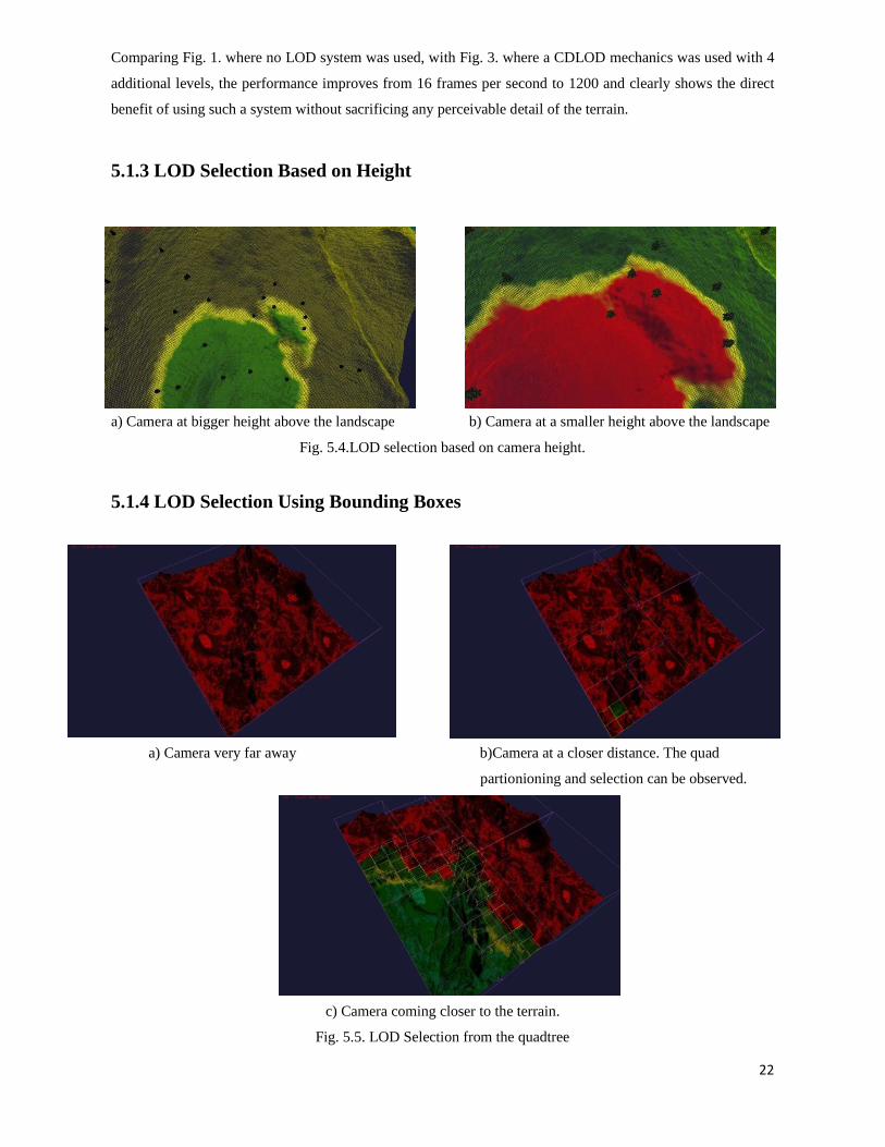
5.1.3 LOD Selection Based on Height
a) Camera at bigger height above the landscape b) Camera at a smaller height above the landscape
Fig. 5.4.LOD selection based on camera height.
5.1.4 LOD Selection Using Bounding Boxes
a) Camera very far away b)Camera at a closer distance. The quad
partionioning and selection can be observed.
c) Camera coming closer to the terrain.
Fig. 5.5. LOD Selection from the quadtree

23
a) Node size of 64 units b) Node size of 8 units
Fig. 5.6. Partinioning control.
5.1.5 Morphing between LOD levels
The morphing between the LOD levels is performed in the vertex shader as described in chapter 3 and 4. A
comparisson between the result obtained in the application and the original implementation by Strugar
F.(2010) can be seen below:
a) Morphing as seen in the original CDLOD b) Morphing as seen in the current application
implementation by Strugar F., 2010
Fig. 5.7. Morphing of LOD levels

24
5.2 Stereoscopic visualization
The stereoscopic implementation is based on the algorithms and methods described in chapter 3 and
4. In order for it to work it requires special hardware. By default, if no such harware exists, the application
will render in a monoscopic context.
a) Scene rendered using the left eye projection b) Scene rendered using the right eye projection
c) Both eyes rendered (left + right) as seen on the monitor without glasses.
Fig. 5.8. Stereoscopic rendering

25
5.3 Performance results
5.3.1 GPU Performance
GPU Model FPS in stereo 3D
- normal scenario
FPS in stereo 3D
- only terrain
FPS in 2D
- normal scenario
FPS in 2D
- only terrain
GPU usage
3D /2D
nVidia GT 555m 60 60(66% GPU) 96 325(76%GPU) 82% / 89%
Nvidia GTX 580 60 - - - 25% / -
nVidia GTX 590 60 60 (15% GPU) 360 1000 60% / 92%
nVidia GTX 660 185 - 150 - -
nVidia GTX 670 120 - 208 - 51% / 88%
nVidia GTX 680ti 270 - 270 - -
- normal scenario = terrain mesh + vegetation using the Instanced Cloud Reduction method
- only terrain = terrain mesh
The above table presents the performance hit on current generation GPUs. The values from the table
were provided by the users from the GeForce Forums, upon being provided with a test build of the
application.
One important thing to mention is when rendering in stereoscopic 3D, the driver automatically caps (turns
VSYNC ON) the framerate to the refresh rate of the monitor. It is possible, however, to disable this by force
from the driver. The bold entries are the results of tests conducted in all scenarios by the author of this paper.
It can be clearly seen that using a mobile GPU provides different results, as the driver branch differs.
Normally, because the all the geometry is rendered two times the performance hit should be around 50%.
However as it can be seen, this is not always true. In some cases the performance seems to be better when the
stereo renderer it is used.
The dataset used in all the tests consists of: 256 x256 grid size. Grid scale 4.0. Total mesh size in
units: 1024x1024. Height scale factor: 250). CDLOD with 3 additional levels that break at 64, 256, 2048
distance in units.
5.3.2 CPU Load
CPU Model Number of Physical
Cores (no HT)
Utilization during
runtime
Intel i5 2430M @ 2.4 Ghz 2 25%
Intel i5 3570k @ 3.8 Ghx 4 25%

26
The CPU usage measurements were done on two chips: one being a mobile processor and the
secondary a desktop one. In both cases the same amount of utilization was seen.
5.3.3 Memory Allocation Performance
Terrain Type Total Program
Allocated Memory
256 x 256 grid size. 64.628 MB
512 x 512 grid size. 77.388 MB
1024 x 1024 grid size. 132.176 MB
2048 x 2048 grid size. 381.832 MB
4096 x 4096 grid size 1.115.220 MB
The values were measured on a Windows platform. The reported allocated memory is done by the
operating system for the whole application and may slightly differ on the Linux platform.

27
6. Conclusions and future work
Procedural terrain generation from heightmaps is still vastly used. Employing a LOD system can save
an application a lot of computational and rendering time, as shown in the Results chapter. By using a LOD
system when rendering a generated terrain mesh the performance of an application can be increased
tremendously, sometimes going from 16fps to even 1000fps, as shown above. The downside of this, is that it
requires additional memory. The CDLOD algorithm implemented vastly improves the performance and the
quality of generated terrain, improving on all the previous LOD algorithms and in the same time being very
flexible. A couple of downsides must be mentioned though. It is limited to only selecting between two LOD
levels. Each heightmap and terrain generation requires finding the optimum parameters for LOD selection
distance (LOD break), size of the grid mesh in order to be effective and thus, sometimes can become tedious.
One of its big advantages is its ability to handle large triangles count and in the current implementation is only
bound by the type of platform is running on in terms of memory allocation. Based on testing, trying to
generate a grid mesh of anything higher than 4096x4096 will always fail with a bad allocation on 32-bit
systems since the operating system cannot allocate more than 2 GB for an application.
The implementation in its current form does not handle terrain streaming since it wasn't in the scope
of the project. However, the current implementation can be vastly improved by:
- improve the implementation to work with any type of grid size, not only square
- using tessellation to further increase polygon count starting from a low resolution grid
- using subdivisions with tessellation to even further improve the quality of the landscape, as described by
Mistal B., 2013.
- using a streaming method as ROAM to handle even larger terrains by updating the vertex buffers in real-
time.
- by adding frustum culling for a real case scenario usage.
The Instance Cloud Reduction algorithm was selected only to help for a better visualization in a
stereoscopic context and was not the main focus of the developed application. The addition of a bigger
number of polygons that are renderer were used as a simulation factor of a real case scenario, where the GPU
has to render millions of triangles per second. However, it can be greatly improved, by adding a LOD
selection mechanism in order to decrease the number of polygons that are visible.

28
7. References
Asirvatham A., and Hoppe H., 2005. GPU Gems 2. Addison-Wesley Professional
Bourke P., 1999. 3D Stereo Rendering Using OpenGL (and GLUT). Available from: ftp://ftp.sgi.com/opengl/ contrib/kschwarz/GLUT_INTRO/SOURCE/PBOURKE/index.html [Last accessed August 2013] Cervin A., 2012. Adaptive Hardware-accelerated Terrain Tessellation. Available from: http://dice.se/wp-content/uploads/adaptive_terrain_tessellation.pdf [Last accessed August 2013]
Gateau S. and Nash S., 2010. Implementing Stereoscopic 3D in Your Applications. Nvidia Corportation. Available from: http://www.nvidia.com/content/GTC-2010/pdfs/2010_GTC2010.pdf [Last accessed August 2013] GeForce Forums., 2013. [Test Request]Stereo 3D OpenGL application. Available from: https://forums.geforce.com/default/topic/572432/3d-vision/-test-request-stereo-3d-opengl-application/ [Last accessed August 2013] Macey J., 2012. Operator overloading and Dynamic Data Structures. Available from: http://nccastaff. bournemouth.ac.uk/jmacey/ASD/slides/Lecture4OperatorsandDynamicDS.pdf[Last accessed August 2013] Mishra A., 2011. Rendering 3D Anaglyph in OpenGL. Available from: http://quiescentspark.blogspot.co.uk/2011/05/rendering-3d-anaglyph-in-opengl.html [Last accessed August 2013]
Rakos D., 2010. Instance culling using geometry shaders. Available from: http://rastergrid.com/blog/2010/02/instance-culling-using-geometry-shaders/ [Last accessed August 2013]
Strugar F., 2010. Continuous Distance-Dependent Level of Detail for Rendering Heightmaps (CDLOD). Available from:http://www.vertexasylum.com/downloads/cdlod/cdlod_latest.pdf [Last accessed August 2013] Ulrich T., 2002. Rendering Massive Terrains using Chunked Level of Detail Control. Available from: http://tulrich.com/geekstuff/sig-notes.pdf [Last accessed August 2013]
Wloka M., 2004. Optimizing the Graphics Pipeline. Nvidia Corporation. Available from: https://developer.nvidia.com/sites/default/files/akamai/gamedev/docs/EG_04_OptimizingGPUPipeline.pdf [Last accessed August 2013] Wolfgang E., and Mistal B., 2013. GPU Terrain Subdivision and Tessellation.GPU Pro 4. A K Peters/ CRC Press.
7.1 Texture References
Dirt texture. Available from: http://www.imageafter.com/dbase/textures/grounds/b1dirt012.jpg [Last accessed August 2013] Grass texture. Available from: http://threeminutevideo.co.uk/wpcontent/themes/kingsize/images/upload/ GrassTexture.jpg [Last accessed August 2013] Rock texture. Available from: http://www.texturex.com/Stone-Textures/TextureX+gravel+texture+rock+gravel +street+sidewalk+grey+concrete+Texture.jpg.php [Last accessed August 2013] Snow texture. Available from: http://farm6.staticflickr.com/5286/5342749399_6ba1d9b685_o.jpg [Last accessed August 2013] Heightmap texture. Available from: http://www.alvaromartin.net/images/surfaceclipmaps/heightmap.jpg [Last accessed August 2013] Heightmap texture. Available from: http://read.pudn.com/downloads38/sourcecode/windows/ opengl/127140/Demos/Fustrums/Textures/Heightmap__.jpg [Last accessed August 2013]

29
Appendix A