procedures for setting advisory speeds on curves · speed, engineering study methods for...

Procedures for SettingAdvisory Speeds on Curves

FHWA Safety Program

http://safety.fhwa.dot.gov

FHWA Safety Program

FHWA-SA-11-22

DisclaimerThe contents of this handbook reflect the views of the authors, who are responsible for the facts and the accuracy of the data published herein. The contents do not necessarily reflect the official view or policies of the Federal Highway Administration (FHWA). This handbook does not constitute a standard, specification, or regulation. It is not intended for construction, bidding, or permit purposes. The engineer in charge of the project was Robert Milstead, P.E. #17172 (Maryland).

NoticeThe United States Government does not endorse products or manufacturers. Trade or manufacturers’ names appear herein solely because they are considered essential to the object of this handbook.

AcknowledgementsThe report that led to the development of this handbook was sponsored by the Texas Department of Transportation and the Federal Highway Administration. The research report was written by Dr. James Bonneson, Mr. Michael Pratt, Mr. Jeff Miles, and Dr. Paul Carlson (1). These researchers are employees with the Texas Transportation Institute (TTI).

Technical Report Documentation Page

1. Report No.

7. Author(s)

17. Key Words

19. Security Clasif. (of this report)

Form DOT F 1700.7 (8-72) Reproduction of completed page authorized

20. Security Clasif. (of this page) 21. No. of Pages 21. Price

4. Title and Subtitle

15. Supplementary Notes

16. Abstract

9. Performing Organization Name and Address

12. Sponsoring Agency Name and Address

5. Report Date

10. Work Unit No. (TRAIS)

13. Type of Report and Period Covered

6. Performing Organization Code

11. Contract or Grant No.

14. Sponsoring Agency Code

8. Performing Organization Report No.

18. Distribution Statement

FHWA-SA-11-22

Procedures for Setting Advisory Speeds on Curves

Project performed for the Federal Highway Administration

Project Title: Curve Advisory Speed Workshops and Demonstrations

Project Manager: Guan Xu

FHWA Technical Panel: Ed Rice, Richard Knoblauch, Kevin J. Sylvester, Joseph Cheung

Horizontal curves are a necessary component of the highway alignment; however, they tend to be associated with a dispro-portionate number of severe crashes. Warning signs are intended to improve curve safety by alerting the driver to a change in geometry that may not be apparent or expected. However, several research projects conducted in the last 20 years have consistently shown that drivers are not responding to curve warning signs or complying with the Advisory Speed plaque. It is estimated that half of all speeding related roadway departure crashes occur on curves. One of the reasons that curves are over-represented in speeding related fatalities is due, in part, to advisory speeds that are not consistent, and therefore, not credible.

A project by Texas Transportation Institute (TTI), Texas Research Project 0-5439 “Identifying and Testing Effective Advisory Speed Setting Procedures”, exemplifies how current procedures for setting advisory speed on curves are not reliable, and has developed new criteria and a new procedure that are more consistent with driver expectation. The new procedure involves the use of an Excel spreadsheet and a handbook for applying the new criteria.

The procedures described in the handbook are intended to improve consistency in advisory speed signing and, hopefully, driver compliance with the advisory speed. The handbook describes; 1) guidelines for determining when an advisory speed is needed; 2) criteria for identifying the appropriate advisory speed; 3) an engineering study method for determining the advi-sory speed; and 4) guidelines for selecting other curve related traffic control devices.

Brudis & Associates, Inc.Science Applications International CorporationTexas Transportation Institute

Federal Highway AdministrationOffice of Safety1200 New Jersey Ave., SEWashington, DC 20590

R. Milstead, X. Qin, B. Katz, J. Bonneson, M. Pratt, J. Miles, and P. Carlson

Traffic Control Devices, Warning Signs, Speed Signs, High-way Curves, Speed Measurement, Trucks, Traffic Speed

No restrictions.

Unclassified Unclassified 44 N/A

June 2011

2. Government Accession No. 3. Recipient’s Catalog No.

October 2009-June 2011

iii

TAble of CoNTeNTS

CHAPTER 1. INTRODUCTION.........................................................................................................1

1.1 Overview ..................................................................................................................................................1

1.2 Purpose and Scope ................................................................................................................................1

CHAPTER 2. CONVEYING CHANGES IN HORIZONTAL ALIGNMENT .............................................2

2.1 Overview ..................................................................................................................................................2

2.2 Horizontal Curve Safety and Operation ................................................................................................2

2.3 Warning Signs for Changes in Horizontal Alignment ...........................................................................4

2.4 Curve Advisory Speed Software ............................................................................................................6

CHAPTER 3. METHODS FOR ESTABLISHING ADVISORY SPEED ....................................................10

3.1 Overview ................................................................................................................................................ 10

3.2 Direct Method ....................................................................................................................................... 11

3.3 Compass Method ................................................................................................................................. 12

3.4 GPS Method .......................................................................................................................................... 18

3.5 Design Method .....................................................................................................................................22

3.6 Ball-Bank Indicator Method .................................................................................................................23

3.7 Accelerometer Method ........................................................................................................................25

3.8 Confirming Speed for Conditions ........................................................................................................28

3.9 Workshops and Webinars ....................................................................................................................28

3.10 Summary ...............................................................................................................................................29

CHAPTER 4. CURVE SIGNING GUIDELINES .................................................................................31

4.1 Overview ................................................................................................................................................ 31

4.2 Guidelines ............................................................................................................................................. 31

REFERENCES ................................................................................................................................35

iv

liST of figureS

Figure 1 Effect of Radius, Tangent Speed, and Vehicle Type on Curve Speed .......................................3

Figure 2 Curve Crash Rate as a Function of Radius ...................................................................................3

Figure 3 Horizontal Alignment Signs and Plaques (MUTCD 2009 Edition) ...............................................5

Figure 4 Curve Advisory Speed (CAS) Software Analysis Worksheet ........................................................7

Figure 5 Location of Critical Portion of Curve ........................................................................................... 13

Figure 6 Curve Advisory Speed (CAS) Software Input Data .................................................................... 16

Figure 7 Curve Advisory Speed (CAS) Software Advisory Speed Calculation ...................................... 17

Figure 8 Effect of Lateral Shift on Travel Path Radius ................................................................................ 17

Figure 9 GPS Method Equipment Setup in Test Vehicle ........................................................................... 19

Figure 10 Texas Roadway Analysis and Measurement Software (TRAMS) Main Panel ..........................20

Figure 11 Import TRAMS Data ......................................................................................................................22

Figure 12 Ball-Bank Indicator .......................................................................................................................24

Figure 13 CurveRite Front Panel ...................................................................................................................26

Figure 14 CurveRite Measurement ..............................................................................................................27

Figure 15 MUTCD 2009 Edition Criteria for the Selection of Horizontal Alignment Sign ...........................32

Figure 16 MUTCD 2009 Edition Criteria for the Typical Spacing of Chevron Alignment Signs on Horizontal Curves ........................................................................................32

Figure 17 MUTCD 2009 Edition Criteria for Advance Placement of Warning Signs .................................33

Figure 18 Curve Advisory Speed (CAS) Software Traffic Control Device Guidance................................34

liST of TAbleS

Table 1 Comparison of the Six Methods for Establishing Curve Advisory Speeds ...............................30

1

CHAPTer 1. iNTroDuCTioN

1.1 OverviewHorizontal curves are a necessary component of the highway alignment; however, they tend to be associated with a disproportionate number of severe crashes. Recently, in the United States, about 33,000 fatalities occur nationwide each year, and about 25 percent of these fatalities occur on horizontal curves (2).

Curve warning signs are intended to improve curve safety by alerting the driver to an upcoming change in geometry that may not be apparent or expected. One or more of the curve warning signs identified in the Manual on Uniform Traffic Control Devices (MUTCD 2009 edition) (3) are typically used to notify drivers. Drivers may also be notified of the need to reduce their speed through the use of an Advisory Speed plaque.

Several research projects conducted in the last 20 years have consistently shown that drivers are not responding to curve warning signs and are not complying with the Advisory Speed plaque. Evidence of this non-responsiveness is supported by the aforementioned curve crash statistics. Chowdhury et al. (4) suggest that current practice in the U.S. for setting advisory speeds is contributing to this lack of compliance and the poor safety record. They advocate the need for a procedure that can be used to: (a) identify when a curve warning sign and advisory speed are needed, and (b) select an advisory speed that is consistent with driver expectation. They also recommend the uniform use of this procedure on a nationwide basis, such that driver respect for curve warning signs is restored and curve safety records are improved.

1.2 Purpose and ScopeThe procedures described in this handbook are intended to improve consistency in curve signing and, subsequently, driver compliance with the advisory speed. The handbook describes guidelines for determining when an advisory speed is needed, criteria for identifying the appropriate advisory speed, engineering study methods for determining the advisory speed, and guidelines for selecting other curve related traffic control devices.

The handbook is to be used by traffic engineers and technicians who are responsible for evaluating and maintaining horizontal curve signing and delineation devices.

The curve advisory speed and other curve related traffic control devices should be checked periodically to ensure that they are appropriate for the prevailing conditions. Changes in the regulatory speed limit, curve geometry, or crash history may require an engineering study to reevaluate the appropriateness of the existing signs and the possible need for additional signs.

2

CHAPTer 2. CoNVeYiNg CHANgeS iN HoriZoNTAl AligNMeNT

2.1 OverviewThis chapter provides a brief overview of topics related to horizontal curve safety, operation, and curve warning signs. It consists of three parts. The first part examines the safety and operation of horizontal curves. The second part reviews the various warning signs that are used to sign horizontal curves. The last part provides an overview of the Curve Advisory Speed (CAS) software that was developed to automate the procedures and criteria described in Chapters 3 and 4, respectively.

Additional background information about curve advisory speed is provided in Bonneson et al. (5). The information in that report examines the objectives of curve signing and the challenges associated with establishing advisory speeds that are uniform among curves and consistent with driver expectation. That report also reviews the various criteria that have been used to set advisory speeds.

2.2 Horizontal Curve Safety and OperationThis part of the chapter examines the factors that influence the safety and operation of horizontal curves. The focus is on factors related to the curve’s geometric design. The relationship between curve design and driver speed choice is described in Section 2.2.1, and the relationship between curve design and crash rate is explored in Section 2.2.2.

2.2.1 Curve Speed

A review of the literature indicates that several variables can have an influence on curve speed. These variables include:

•Radius,

•Superelevation,

•Tangent Speed,

•Vehicle Type,

•Curve Deflection Angle,

•Curve Length,

•Tangent Length,

•Sight Distance,

Of these variables, research indicates that the first five have the most significant effect on curve speed. Using data collected on rural highways in Texas, Bonneson et al. (5) developed a curve speed prediction model that includes sensitivity to these variables. The speeds predicted by this model are shown in Figure 1. The trends shown indicate that the average truck speed equals about 97 percent of the average passenger car speed.

•Grade,

•Vertical Curvature,

•Shoulder Characteristics,

•Edge Drop-off,

•Weather,

•Lighting, and

•Roadway surface, type/condition.

3

Figure 1 – Effect of Radius, Tangent Speed, and Vehicle Type on Curve Speed

The trend lines in Figure 1 indicate that drivers on sharper curves slow from the tangent speed to an acceptable curve speed. The amount of speed reduction increases with decreasing radius. For curves with a 500 ft radius and a 60 mph tangent speed, the reduction is about 10 mph. In contrast, for a 1000 ft radius and 60 mph tangent speed, the reduction is only about 5 mph.

The effect of superelevation rate is not shown in Figure 1; however, the model indicates that curve speed increases about 1.0 mph for every 2.0 percent increase in superelevation.

2.2.2 Curve Safety

Bonneson et al. (5) examined the relationship between curve radius and crash rate using safety relationships documented in the literature (6, 7). These relationships are shown in Figure 2. In this figure, crash rate is defined in terms of crashes per million vehicle miles (crashes/mvm). One trend line represents the combination of fatal and injury crashes. The other trend line represents the combination of fatal, injury, and property-damage-only (PDO) crashes.

The two trend lines in Figure 2 are in fairly good agreement. They indicate that the crash rate increases sharply for curves with a radius of less than 1000 ft. They also indicate that more crashes on sharper curves result in injury or fatality.

Based on the discussion in this and the previous sections, it is likely that the trends in Figure 2 are reflecting driver error while entering or traversing a curve. It is possible that some drivers are distracted or impaired and do not track the curve. It is also possible that some drivers detect the curve but do not correctly judge its sharpness. In both instances, traffic control devices have the potential to improve safety by making it easier for drivers to detect the curve and judge its sharpness.

Figure 2 – Curve Crash Rate as a Function of Radius

a. 85th Percentile Speed. b. Average Speed.

20

25

30

35

40

45

50

55

60

0 500 1000 1500

Radius, ft

85th

% C

urve

Spe

ed, m

ph

Trucks Passenger Cars

85th % Tangent Speed = 40 mph

50 mph

60 mph6% Superelevation

20

25

30

35

40

45

50

55

60

0 500 1000 1500

Radius, ft

Ave

rage

Cur

ve S

peed

, mph

Trucks Passenger Cars

85th % Tangent Speed = 40 mph

50 mph

60 mph

6% Superelevation

0.0

1.0

2.0

3.0

4.0

0 500 1000 1500 2000 2500

Radius, ft

Cra

sh R

ate,

cra

shes

/mvm

85th% tangent speed = 60 mph

Bonneson et al. (5)Fitzpatrick et al. (6)

Fatal + Injury + PDOFatal + Injury

4

2.3 Warning Signs for Changes in Horizontal AlignmentMost transportation agencies use a variety of traffic control devices to inform road users of a change in horizontal alignment. These devices include curve warning signs, delineation devices, and pavement markings. The focus of this part of the chapter is on curve warning signs; however, conditions where other traffic control devices may be helpful are also identified.

2.3.1 Horizontal Alignment Warning Signs

The MUTCD 2009 edition (3) identifies a variety of warning signs that can be used where the horizontal alignment changes in an unexpected or restrictive manner. These signs are shown in Figure 3. The recommended signs include:

•Turn (W1-1),

•Curve (W1-2),

•Combination Horizontal Alignment/Advisory Speed Signs (W1-1a, W1-2a),

•Reverse Turn (W1-3),

•Reverse Curve (W1-4),

•Winding Road (W1-5),

•One-Direction Large Arrow Sign (W1-6),

•Chevron Alignment Sign (W1-8),

•Combination Horizontal Alignment/Intersection Signs (W1-10 Series, W1-10, W1-10a, W1-10b, W1-10c, W1-10d, and W1-10e)

•Hairpin Curve (W1-11),

•270-degree Loop (W1-15),

•Truck Rollover (W1-13),

•Advisory Speed Plaque (W13-1P),

•Advisory Exit and Ramp Speed Signs (W13-2 and W13-3), and

•Combination Horizontal Alignment/Advisory Exit and Ramp Speed Signs (W13-6 and W13-7).

5

Figure 3 – Horizontal Alignment Signs and Plaques (MUTCD 2009 Edition)

Compared to the MUTCD 2003 edition (8), the MUTCD 2009 edition (3) has three changes of the sign designation: 1) Combination Horizontal Alignment/Intersection Sign (W1-10) is expanded to include an additional series (W1-10a through W1-10e). This change offers more symbol designs to approximate the configuration of the intersecting roadway. 2) The Advisory Curve Speed Sign (W13-5 in MUTCD 2003 edition) is no longer used as a standard sign. 3) Combination Horizontal Alignment/Advisory Exit and Ramp Speed Signs (W13-6 and W13-7) are added into the horizontal alignment sign category.

The previous versions of the MUTCD criterion regarding the use of horizontal alignment warning signs can best be described as flexible. It encouraged engineers to base their signing decisions on engineering studies and judgment. However, this flexibility had the disadvantage of occasionally promoting inconsistencies in the application of traffic control devices. Inconsistent device application makes it difficult for drivers to develop reasonable expectancies and, consequently, promotes a disrespect of the device and mistrust of its message. The Advisory Speed plaque is perhaps one of best examples of the consequences of inconsistent sign usage. Research has found it to be among the more disrespected traffic control devices (9).

W1-2 W1-3 W1-4W1-1 W1-1a W1-2a

W1-15 W13-1P W13-2 W13-3

W1-5 W1-6 W1-8 W1-10 W1-10bW1-10a

W1-11 W1-13W1-10eW1-10c W1-10d

Note: Turn arrows and reverse turn arrows may be substituted for the curve arrows and reverse curve arrows on the W1-10 series signs where appropriate.

W13-6 W13-7

6

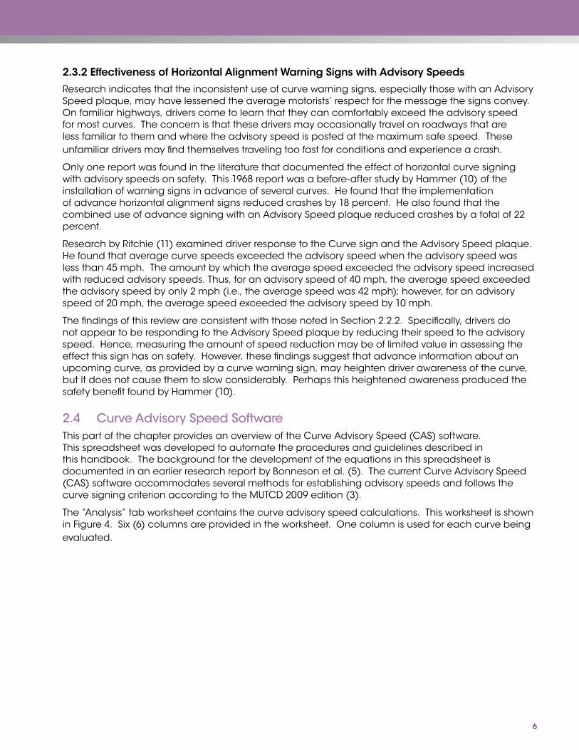
2.3.2 Effectiveness of Horizontal Alignment Warning Signs with Advisory Speeds

Research indicates that the inconsistent use of curve warning signs, especially those with an Advisory Speed plaque, may have lessened the average motorists’ respect for the message the signs convey. On familiar highways, drivers come to learn that they can comfortably exceed the advisory speed for most curves. The concern is that these drivers may occasionally travel on roadways that are less familiar to them and where the advisory speed is posted at the maximum safe speed. These unfamiliar drivers may find themselves traveling too fast for conditions and experience a crash.

Only one report was found in the literature that documented the effect of horizontal curve signing with advisory speeds on safety. This 1968 report was a before-after study by Hammer (10) of the installation of warning signs in advance of several curves. He found that the implementation of advance horizontal alignment signs reduced crashes by 18 percent. He also found that the combined use of advance signing with an Advisory Speed plaque reduced crashes by a total of 22 percent.

Research by Ritchie (11) examined driver response to the Curve sign and the Advisory Speed plaque. He found that average curve speeds exceeded the advisory speed when the advisory speed was less than 45 mph. The amount by which the average speed exceeded the advisory speed increased with reduced advisory speeds. Thus, for an advisory speed of 40 mph, the average speed exceeded the advisory speed by only 2 mph (i.e., the average speed was 42 mph); however, for an advisory speed of 20 mph, the average speed exceeded the advisory speed by 10 mph.

The findings of this review are consistent with those noted in Section 2.2.2. Specifically, drivers do not appear to be responding to the Advisory Speed plaque by reducing their speed to the advisory speed. Hence, measuring the amount of speed reduction may be of limited value in assessing the effect this sign has on safety. However, these findings suggest that advance information about an upcoming curve, as provided by a curve warning sign, may heighten driver awareness of the curve, but it does not cause them to slow considerably. Perhaps this heightened awareness produced the safety benefit found by Hammer (10).

2.4 Curve Advisory Speed SoftwareThis part of the chapter provides an overview of the Curve Advisory Speed (CAS) software. This spreadsheet was developed to automate the procedures and guidelines described in this handbook. The background for the development of the equations in this spreadsheet is documented in an earlier research report by Bonneson et al. (5). The current Curve Advisory Speed (CAS) software accommodates several methods for establishing advisory speeds and follows the curve signing criterion according to the MUTCD 2009 edition (3).

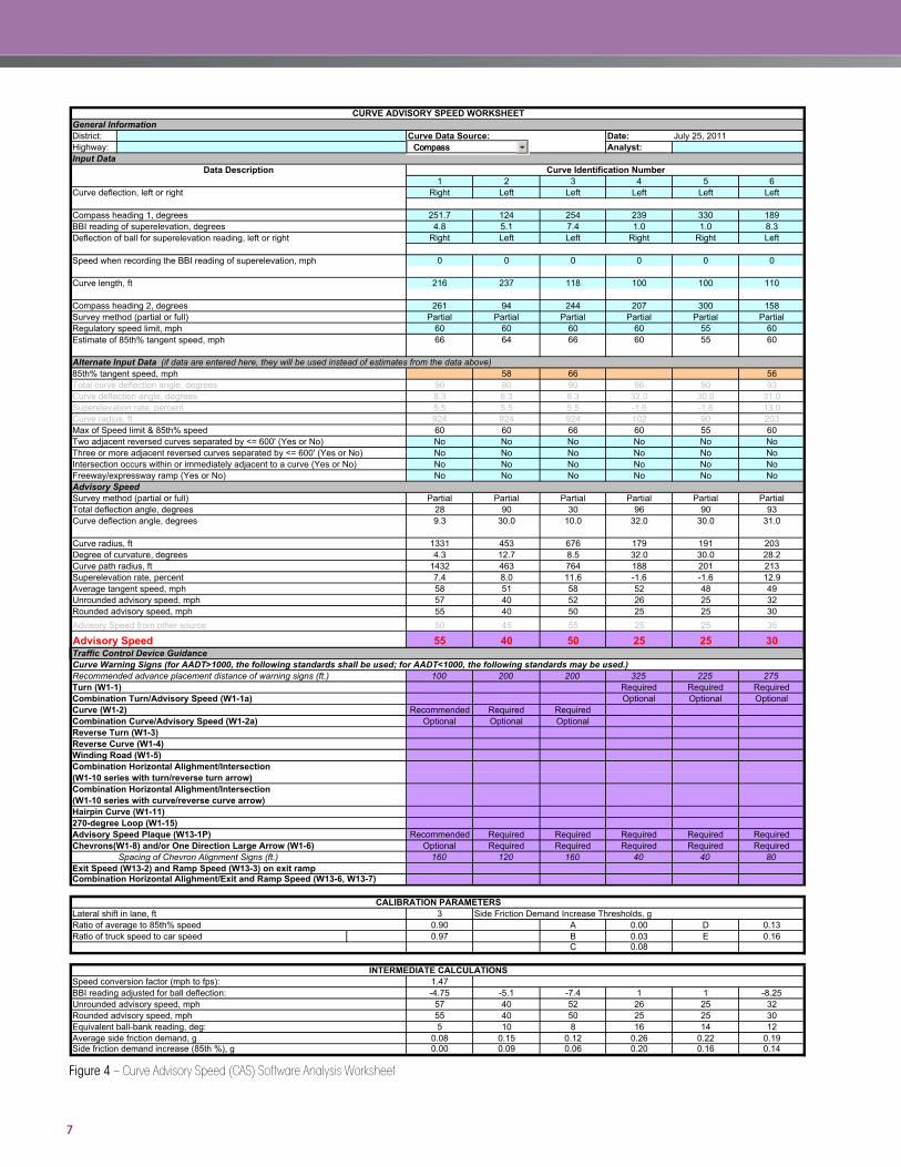
The “Analysis” tab worksheet contains the curve advisory speed calculations. This worksheet is shown in Figure 4. Six (6) columns are provided in the worksheet. One column is used for each curve being evaluated.

7

Figure 4 – Curve Advisory Speed (CAS) Software Analysis Worksheet

General InformationDistrict: Curve Data Source: Date:Highway: Analyst:Input Data

1 2 3 4 5 6Curve deflection, left or right Right Left Left Left Left Left

Compass heading 1, degrees 251.7 124 254 239 330 189BBI reading of superelevation, degrees 4.8 5.1 7.4 1.0 1.0 8.3

Right Left Left Right Right Left

0 0 0 0 0 0

Curve length, ft 216 237 118 100 100 110

Compass heading 2, degrees 261 94 244 207 300 158Survey method (partial or full) Partial Partial Partial Partial Partial PartialRegulatory speed limit, mph 60 60 60 60 55 60Estimate of 85th% tangent speed, mph 66 64 66 60 55 60

Alternate Input Data (if data are entered here, they will be used instead of estimates from the data above)85th% tangent speed, mph 58 66 56Total curve deflection angle, degrees 90 90 90 96 90 93Curve deflection angle, degrees 8.3 8.3 8.3 32.0 30.0 31.0Superelevation rate, percent 5.5 5.5 5.5 -1.6 -1.6 13.0Curve radius, ft 924 924 924 102 90 203Max of Speed limit & 85th% speed 60 60 66 60 55 60Two adjacent reversed curves separated by <= 600' (Yes or No) No No No No No NoThree or more adjacent reversed curves separated by <= 600' (Yes or No) No No No No No NoIntersection occurs within or immediately adjacent to a curve (Yes or No) No No No No No NoFreeway/expressway ramp (Yes or No) No No No No No NoAdvisory Speed Survey method (partial or full) Partial Partial Partial Partial Partial PartialTotal deflection angle, degrees 28 90 30 96 90 93Curve deflection angle, degrees 9.3 30.0 10.0 32.0 30.0 31.0

Curve radius, ft 1331 453 676 179 191 203Degree of curvature, degrees 4.3 12.7 8.5 32.0 30.0 28.2Curve path radius, ft 1432 463 764 188 201 213Superelevation rate, percent 7.4 8.0 11.6 -1.6 -1.6 12.9Average tangent speed, mph 58 51 58 52 48 49Unrounded advisory speed, mph 57 40 52 26 25 32Rounded advisory speed, mph 55 40 50 25 25 30Advisory Speed from other source 50 45 55 25 25 35

Advisory Speed 55 40 50 25 25 30Traffic Control Device Guidance

Curve Identification Number

Deflection of ball for superelevation reading, left or right

Speed when recording the BBI reading of superelevation, mph

CURVE ADVISORY SPEED WORKSHEET

July 25, 2011

Data Description

Compass

Traffic Control Device GuidanceCurve Warning Signs (for AADT>1000, the following standards shall be used; for AADT<1000, the following standards may be used.)Recommended advance placement distance of warning signs (ft.) 100 200 200 325 225 275Turn (W1-1) Required Required RequiredCombination Turn/Advisory Speed (W1-1a) Optional Optional OptionalCurve (W1-2) Recommended Required RequiredCombination Curve/Advisory Speed (W1-2a) Optional Optional OptionalReverse Turn (W1-3)Reverse Curve (W1-4)Winding Road (W1-5)Combination Horizontal Alighment/Intersection(W1-10 series with turn/reverse turn arrow)Combination Horizontal Alighment/Intersection(W1-10 series with curve/reverse curve arrow)Hairpin Curve (W1-11)270-degree Loop (W1-15)Advisory Speed Plaque (W13-1P) Recommended Required Required Required Required RequiredChevrons(W1-8) and/or One Direction Large Arrow (W1-6) Optional Required Required Required Required Required

Spacing of Chevron Alignment Signs (ft.) 160 120 160 40 40 80Exit Speed (W13-2) and Ramp Speed (W13-3) on exit rampCombination Horizontal Alighment/Exit and Ramp Speed (W13-6, W13-7)

Lateral shift in lane, ft 3 Side Friction Demand Increase Thresholds, gRatio of average to 85th% speed 0.90 A 0.00 D 0.13Ratio of truck speed to car speed 0.97 B 0.03 E 0.16

C 0.08

Speed conversion factor (mph to fps): 1.47BBI reading adjusted for ball deflection: -4.75 -5.1 -7.4 1 1 -8.25Unrounded advisory speed, mph 57 40 52 26 25 32Rounded advisory speed, mph 55 40 50 25 25 30Equivalent ball-bank reading, deg: 5 10 8 16 14 12Average side friction demand, g 0.08 0.15 0.12 0.26 0.22 0.19Side friction demand increase (85th %), g 0.00 0.09 0.06 0.20 0.16 0.14

CALIBRATION PARAMETERS

INTERMEDIATE CALCULATIONS

Compass

8

The spreadsheet can be used with six types of input data. One method is based on data obtained from a survey of the curve using the Compass Method. This method is described in Chapter 3. The drop-down list located in cell F5 is used to specify this method by selecting “Compass,” as shown in Figure 4. The data from the Compass Method are entered in the cells that have a light blue shaded background in the rows 9 through 21 and are designated “input data” cells. If the 85th percentile tangent speed is not known, then this cell should be left blank, and row 25 and the estimate in the row 22 (or the speed limit in the row 21, whichever is larger) will be used as the 85th percentile speed. The cell in the row 25 (orange shaded) is optional to input the 85th percentile speed of free-flowing passenger cars on the tangent prior to the curve. The information in the rows 31 to 34 (light blue shaded) are required to account for special roadway configuration.

The second and third methods of data input are based on describing the curve deflection angle, superelevation rate, and radius. These data can be obtained from the GPS Method or the Design Method, as described in Chapter 3. The use of either of these methods is specified with the drop-down list located in cell F5 by selecting “GPS” or “Design.” The data from the GPS Method or the Design Method are entered in the light blue shaded cells in the row 21 and 26 through 29. If the 85th percentile tangent speed is not known, then this cell should be left blank, and the estimate in the row 22 (or the speed limit in the row 21, whichever is larger) will be used as the 85th percentile speed. The cell in the row 25 (orange shaded) is optional to input the 85th percentile speed of free-flowing passenger cars on the tangent prior to the curve. The information in the rows 31 to 34 (light blue shaded) are required to account for special roadway configuration.

The fourth, fifth and sixth methods of data input are based on other methods, such as the Direct Method, the Ball-Bank Indicator Method, and the Accelerometer Method, as described in Chapter 3. The use of any of these methods is specified with the drop-down list located in cell F5 by selecting “Direct,” “Ball-Bank Indicator,” or “Accelerometer.” The advisory speed established by the other method is entered directly in the light blue shaded cells in the row 48. The cell in the row 21 (regulatory speed limit) is required to apply MUTCD 2009 edition (3) signing criteria. The information in the rows 31 to 34 (light blue shaded) are required to account for special roadway configuration. It is optional to input the 85th percentile speed of free-flowing passenger cars on the tangent prior to the curve in the cell in the 25 (orange shaded). If the 85th percentile speed is not known, then this cell should be left blank, and the estimate in the row 22 (or the speed limit in the row 21, whichever is larger) will be used as the 85th percentile speed. The information, total curve deflection angle, in the cell in the row 26 (light blue shaded) is used for curve warning sign determination process.

The cells in the rows 36 to 46, which do not have background shading, contain equations for the first three input methods. The basis for each equation is documented in Bonneson et al. (5). These equations document the analysis of advisory speed for each of the six curves. The purple shaded cell in the row 49 is the advisory speed established by the applied method.

The purple shaded cells in the rows 54 to 73 of the spreadsheet document the traffic control device guidance. The criterion described in Chapter 4 of this manual and the MUTCD 2009 edition (3) are used to calculate the information that is summarized in this section of the spreadsheet. If cells are blank in this section of the spreadsheet then the traffic control device for that column is not required for that curve.

9

The cells in the rows 94 to 107 of the spreadsheet contain many parameters that control the computations. The default model used for calculating the advisory speed is based on the average truck speed (5). The corresponding formulation is as follows:

Vc,a = ( 15.0Rp (0.112 – 0.00066Vt,a + 0.000091V 2t,a – 0.0108Itk + е/100) )0.5

≤ Vta1 + 0.00136Rp

where,

Rp = travel path radius, ft;

Vc,85 = 85th percentile curve speed, mph;

Vt,85 = 85th percentile tangent speed, mph;

Vc,a = average curve speed, mph;

Vt,a = average tangent speed, mph;

е = superelevation rate, percent; and

Itk = indicator variable for trucks (= 1.0 if modelis used to predict truck speed; 0.0 otherwise)

Note that the default model used in the Curve Advisory Speed (CAS) software assumes to use the estimated average truck speed to establish the advisory speed for a particular curve. This is a conservative approach proposed by TTI to ensure safety. However, there is no consensus or agreement among various transportation practitioners on whether to use passenger car vs. truck and average speeds vs. 85th percentile speeds as the criteria to establish advisory speeds. Therefore, it is suggested, before modifying these parameters in the spreadsheet, to carefully read through the report by Bonneson et al. (5) and think about if the default assumption matches your engineering experience and judgment.

If other criteria are chosen to establish the advisory speed, the parameters can be modified. For example, if the 85th percentile speed is preferred to be used as the advisory speed, the formulation shall be changed to the following equation.

If other criteria are chosen to establish the advisory speed, the parameters can be modified. For example, if the 85th percentile speed is preferred to be used as the advisory speed, the formulation shall be changed to the following equation.

Vc,85 = ( 15.0Rp (0.196 – 0.00106Vt,85 + 0.000073V 2t,85 – 0.0150Itk + е/100) )0.5

≤ Vt851 + 0.00109Rp

The formulation is changed through the modification in the cell in the row 103.

If the passenger car speed is preferred to be used to establish the advisory speed, due to, low volume of trucks or low truck crash rate, the value in the cell in the row 97 shall be changed to 1.0 and Itk in the formulation shall be set to 0.0.

10

CHAPTer 3. MeTHoDS for eSTAbliSHiNg ADViSorY SPeeD

3.1 OverviewSix (6) methods for establishing advisory speed are described in this chapter. The advantages and disadvantages of each method will also be discussed. The appropriate selection and application of the methods shall be considered to provide a uniform and consistent advisory speed among curves.

These methods are the most widely used or newly proposed and promising methods related to curve advisory speed determination that are accepted by transportation professionals and researchers.

The methods are all based on the premise that the selection of an advisory speed and the need for various curve warning signs should be based on the “critical” portion of the curve. The critical portion of the curve is defined as the section that has a radius and superelevation rate that combine to yield the largest side friction demand. Through this definition, the procedure is applicable to curves that have a constant radius, compound curvature, or spiral transitions.

Any of the following six (6) methods can be used to determine the curve advisory speed if used appropriately:

•Direct Method,

•TTI Curve Speed Model - Compass Method,

•TTI Curve Speed Model - Global Positioning System (GPS) Method,

•TTI Curve Speed Model - Design Method,

•Ball-Bank Indicator Method, and

•Accelerometer Method.

The Direct Method is based on field measurements of traffic speeds in the curve. The Compass Method is based on a single-pass survey technique using a digital compass, distance measuring instrument and ball-bank indicator to estimate the curve radius and deflection angle. The GPS Method is also based on a single pass survey using a GPS receiver and software to compute curve radius and deflection angle. The Design Method is useful when the radius and deflection angle are available from as built plans. The Ball-Bank Indicator Method is based on a set of field driving tests to record a ball-bank indicator reading using a ball-bank indicator and a speedometer. The Accelerometer Method is based on a set of field driving tests to measure average maximum lateral gravitational force using an electronic accelerometer device and a GPS receiver.

The six (6) methods are categorized into two general groups. The Direct Method, the Compass Method, the GPS Method, and the Design Method determine advisory speeds based on measured operating speeds or estimated operating speeds given curve geometry. The Ball-Bank Indicator Method and the Accelerometer Method determine advisory speeds based on lateral acceleration.

Regardless of which method is being used, the procedure for implementing each method consists of three steps. During the first step, measurements are taken in the field. During the second step, the measurements are used to compute the advisory speed. During the last step, the recommended advisory speed is confirmed through a field trial run. The first two steps are described for each method in the following sections. The last step is common to each method and will be described in the last section of the chapter.

As mentioned, these six (6) methods are the most widely used or newly proposed and promising methods. There may be other methods which have been used to determine curve advisory speeds, for example, Driver Comfort Speed Method and AASHTO’s Geometric Design Method.

11

The Driver Comfort Speed Method is the oldest empirical method used for determining advisory speeds. It was defined in the 1930s as that “which causes an occupant of the vehicle to feel an outward pitch” and later refined to be “that speed at which the driver’s judgment recognized incipient instability.” The method is very subjective and provides inconsistent results.

The AASHTO’s Geometric Design Method is based on the following equation (12) derived from the laws of mechanics and used during the traditional highway design process. The actual value of the side friction factor is different for different ranges of advisory speed and there was variation for speed and side friction relationship based on the field results (12).

V 2 = 15(0.01е + f )Rwhere,

V = advisory speed, mph;

е = superelevation, percent;

f = side friction factor; and

R = radius curvature, ft.

This report will not further discuss the Driver Comfort Speed Method, the AASHTO’s Geometric Design Method and other non-widely used methods hereafter.

3.2 Direct MethodThe Direct Method is based on the field measurement of vehicle speeds on the subject curve. There has been widespread discussion about how to choose the advisory speed given direct measurements of curve speed distribution and vehicle classification. The disagreement is mainly on which speed statistic and which type of vehicle should be used.

•Using 85th percentile, average, or median speeds?

•Based on speeds of passenger cars, trucks, or all vehicles?

The MUTCD 2003 edition (8) recommends the advisory speed be the 85th-percentile speed of free-flowing traffic. It also stated that the 85th-percentile speed on curves approximates a 16-degree ball-bank indicator reading and is the speed at which most drivers’ judgment recognizes incipient instability along a ramp or curve.

However, the MUTCD 2009 edition (3) no longer provides explicit support to use 85th-percentile free-flowing speed as the advisory speed. The manual mentions that research has shown that drivers often exceed existing posted advisory curve speeds by 7 to 10 mph. The MUTCD 2009 edition (3) references posted advisory speeds determined by ball-bank values of 16, 14, and 12 degrees to address such driver behavior.

Bonneson et al. (5) recommended that the advisory speed should be based on the average speed selected by truck drivers. This speed is 2 or 3 mph below that of passenger car drivers and thereby, represents about the 40th percentile car driver. It is rationalized that driver speed choice on sharp horizontal curves is largely influenced by safety concerns. Thus, the advisory speed should be conservative such that it informs drivers of the speed that is considered appropriate for the unfamiliar driver. Given that the speed distribution is approximately normal, the speed most commonly chosen by drivers is the average speed.

Using the Direct Method will allow the engineer to set the advisory speed at the speed at which drivers are driving the curve and for the type of vehicle that the curve requires.

12

3.2.1 Conducting Field Measurements

The speed of free-flowing passenger cars should be measured at the middle of the curve in one direction of travel. A free-flowing vehicle will be at least three (3) seconds behind the previous vehicle. If a radar speed meter is used, then data collection can be discontinued after the speed of 125 cars has been measured or two hours have elapsed, whichever occurs first. If a traffic counter/classifier is used, then data collection can be discontinued after the speed of 125 cars has been measured or four hours have elapsed, whichever occurs first.

If the roadway is divided or if conditions suggest the need to consider direction of travel, the measurements should be repeated for both directions of travel. When two (2) or more curves are present, each curve should be surveyed separately in this step; however, if they are separated by a tangent section of 600 feet or less, one sign should be selected to apply to all curves.

The arithmetic average and the 85th percentile of the measured speeds should be computed for each direction of travel at each curve studied to determine the unrounded advisory speed.

3.2.2 Determining the Advisory Speed

Depending on the criteria chosen, the unrounded advisory speed is obtained by either calculating the 85th percentile passenger car speed or multiplying the average passenger car speed by 0.97 to obtain an estimate of the average truck speed. (Bonneson et al. (5)).

Furthermore, Bonneson et al. (5) proposed a rounding technique to determine the advisory speed. First add 1.0 mph to the unrounded advisory speed and then round the sum down to the nearest 5 mph increment to obtain the advisory speed. This technique yields a conservative estimate of the advisory speed by effectively rounding curve speeds that end in 4 or 9 up to the next higher 5 mph increment, while rounding all other speeds down. For example, applying this rounding technique to a curve speed of 54, 55, 56, 57, or 58 mph yields an advisory speed of 55 mph.

Each curve should be evaluated separately in this step; however, when two (2) or more curves are separated by a tangent of 600 feet or less, one (1) sign should apply for all curves. In this case, the Advisory Speed plaque should show the value for the curve having the lowest advisory speed in the series.

For undivided roadways, if an advisory speed is determined to be needed for one curve travel direction but not for the opposite curve travel direction, then only one direction of the curve should be posted with the advisory speed.

3.3 Compass MethodThe Compass Method is based on a single-pass survey technique using a digital compass, distance measuring instrument and ball-bank indicator to estimate the curve geometry. Bonneson et al. (5) proposed a speed-prediction model to compute the average truck speed given the curve geometry. This speed then becomes the basis for establishing the advisory speed.

The procedure for implementing the Compass Method is based on compass heading and curve length measurements taken at the critical portion of the curve or sharpest point of the curve. When spiral transitions or compound curves are present, this critical portion of the curve is typically found in the middle third of the curve, as shown in Figure 5. If the curve is truly circular for its entire length, then measurements made in the middle third will yield the same radius estimate as those made in other portions of the curve.

13

Figure 5 – Location of Critical Portion of Curve

The deflection angle associated with the critical portion is referred to as the “partial deflection angle.” The curve length associated with the critical portion is referred to as the “partial curve length.”

To ensure reasonable accuracy in the model estimates using this method, the total curve length should be 200 ft or more and the partial curve length should be 70 ft or more. Also, the curve deflection angle should be 12 degrees or more and the partial curve deflection angle should be 4 degrees or more. A curve with a deflection angle of less than 12 degrees will rarely justify curve warning signs.

The Compass Method allows the engineer to only drive the curve one time; however, this method should only be used on very low volume roads because this method requires stopping the vehicle in the travel lane.


In the first step of the procedure, the technician travels through the subject curve and makes a series of measurements. These measurements include:

•curve deflection in direction of travel (i.e., left or right);

•heading at the “1/3 point” (i.e., a point that is located along the curve at a distance equal to 1/3 of curve length and measured from the beginning of the curve);

•ball-bank reading of curve superelevation rate at the “1/3 point”;

• length of curve between the “1/3” and “2/3” points;

•heading at the “2/3 point“; and

•85th percentile speed (can be estimated using the regulatory speed limit).

These measurements may require two persons in the test vehicle, a driver and a recorder. However, with some practice or through the use of a voice recorder, it is possible that the driver can also serve as the recorder such that a second person is not needed. The next two subsections describe the procedure for making the aforementioned field measurements.

1/3 Curve Length

1/3 Curve Length

1/3 Curve Length

Partial De�ection

Angle

Compass Heading 1

Compass Heading 2

0

0

270

270

180

180

90

90

Partial Deflection Angle = Compass Heading 2 - Compass Heading 1

= 160 - 100

= 60 degrees

14

If the road is divided or if conditions suggest the need for separate consideration of each travel direction, the measurements should be repeated for the opposing direction of travel. If multiple curves are present, each curve should be evaluated separately in this step; however, when two (2) or more curves are separated by a tangent of 600 feet or less, one (1) sign should apply for all curves.

3.3.1.1 Equipment Setup

The test vehicle will need to be equipped with the following three devices:

•digital compass,

•distance-measuring instrument (DMI), and

•ball-bank indicator (BBI).

The digital compass heading calculation should be based on global positioning system (GPS) technology with a position-accuracy of 10 feet or less 95 percent of the time and a position update interval of one (1) second or less. It must also have a precision of 1 degree (i.e., provide readings to the nearest whole degree).

The compass should be installed in the vehicle in a location that is easily accessed and in the recorder’s field of view. The type of mounting apparatus needed may vary; however, the compass should be firmly mounted so that it cannot move while the test vehicle is in motion.

The DMI is used to measure the length of the curve. It should have a precision of 1 ft (i.e., provide readings to the nearest whole foot). The DMI can also be used to: (1) locate a specific curve (in terms of travel distance from a known reference point), and (2) verify the accuracy of the test vehicle’s speedometer. The DMI can be mounted in the vehicle, but should be removable such that it can be hand-held during the test run.

The ball-bank indicator must have a precision of at least one (1) degree (i.e., provide readings to the nearest whole degree). Indicators with less precision (e.g., 5 degree increments) cannot be used with this method. The indicator should be installed along the center of the vehicle in a location that is easily accessed and in the recorder’s field of view. The center of the dash is the recommended position because it allows the driver to observe both the road and the indicator while traversing the curve. The type of mounting apparatus needed may vary; however, the ball-bank indicator should be firmly mounted so that it cannot move while the test vehicle is in motion.

To ensure proper operation of the devices, it is important that the following steps are taken before conducting the test runs:

• Inflate all tires to a pressure that is consistent with the vehicle manufacturer’s specification.

•Calibrate the test vehicle’s DMI.

•Calibrate the ball bank indicator.

The instruction manual should be consulted for specific details about the calibration process for the DMI and the ball-bank indicator.

15

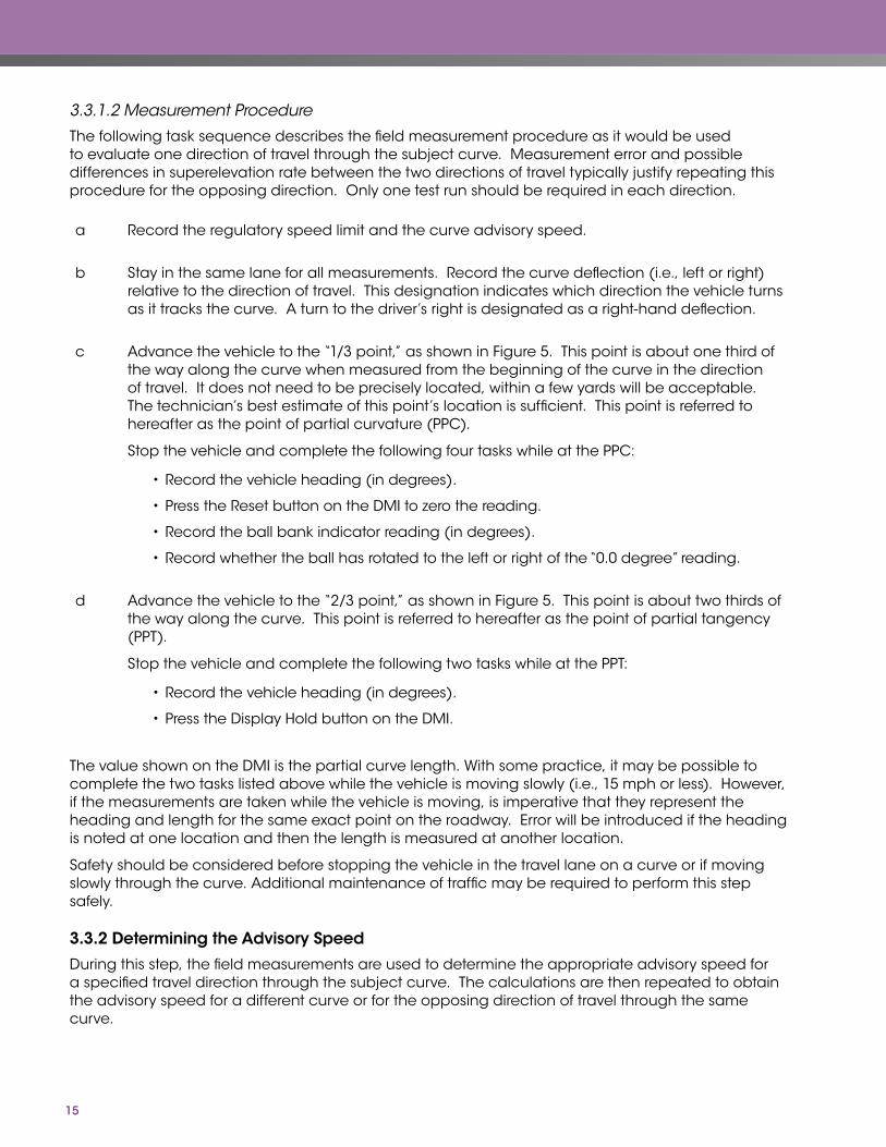
3.3.1.2 Measurement Procedure

The following task sequence describes the field measurement procedure as it would be used to evaluate one direction of travel through the subject curve. Measurement error and possible differences in superelevation rate between the two directions of travel typically justify repeating this procedure for the opposing direction. Only one test run should be required in each direction.

a Record the regulatory speed limit and the curve advisory speed.

b Stay in the same lane for all measurements. Record the curve deflection (i.e., left or right) relative to the direction of travel. This designation indicates which direction the vehicle turns as it tracks the curve. A turn to the driver’s right is designated as a right-hand deflection.

c Advance the vehicle to the “1/3 point,” as shown in Figure 5. This point is about one third of the way along the curve when measured from the beginning of the curve in the direction of travel. It does not need to be precisely located, within a few yards will be acceptable. The technician’s best estimate of this point’s location is sufficient. This point is referred to hereafter as the point of partial curvature (PPC).

Stop the vehicle and complete the following four tasks while at the PPC:

•Record the vehicle heading (in degrees).

•Press the Reset button on the DMI to zero the reading.

•Record the ball bank indicator reading (in degrees).

•Record whether the ball has rotated to the left or right of the “0.0 degree” reading.

d Advance the vehicle to the “2/3 point,” as shown in Figure 5. This point is about two thirds of the way along the curve. This point is referred to hereafter as the point of partial tangency (PPT).

Stop the vehicle and complete the following two tasks while at the PPT:

•Record the vehicle heading (in degrees).

•Press the Display Hold button on the DMI.

The value shown on the DMI is the partial curve length. With some practice, it may be possible to complete the two tasks listed above while the vehicle is moving slowly (i.e., 15 mph or less). However, if the measurements are taken while the vehicle is moving, is imperative that they represent the heading and length for the same exact point on the roadway. Error will be introduced if the heading is noted at one location and then the length is measured at another location.

Safety should be considered before stopping the vehicle in the travel lane on a curve or if moving slowly through the curve. Additional maintenance of traffic may be required to perform this step safely.


During this step, the field measurements are used to determine the appropriate advisory speed for a specified travel direction through the subject curve. The calculations are then repeated to obtain the advisory speed for a different curve or for the opposing direction of travel through the same curve.

16

Initially, the data collected are entered in the Analysis worksheet of the Curve Advisory Speed (CAS) software. The entry of data for example curve “47R” is shown in Figure 6. The measurements taken at this curve are shown in the column headed by the curve’s identification number. The curve deflected to the right, relative to the direction of travel during curve measurement.

The compass heading at the first “1/3 point” was 251 degrees. A ball-bank indicator reading of 4.0 degrees was noted at this point. The ball deflected to the right of the “0.0 degrees” tick mark. This direction indicates that a positive (i.e., beneficial) superelevation is provided along the curve. The vehicle was stopped for these two measurements, so the vehicle speed was input as “0 mph” when the ball-bank indicator was read.

A curve length of 201 ft was measured at the “2/3 point.” The compass heading at this point was 281 degrees. Finally, the regulatory speed limit of 60 mph is entered into the spreadsheet.

Figure 6 – Curve Advisory Speed (CAS) Software Input Data

The speed limit is used to estimate the 85th percentile speed on the highway tangents in the vicinity of the curve. If the 85th percentile tangent speed is known, then it can be directly entered in the first row of the Alternate Input Data section of the worksheet (i.e., the fifth row from the bottom, in Figure 6). If a value is entered in the Alternate Input Data section, then it will be used instead of the value estimated using the field measurements entered in the Input Data section. This priority is extended to the direct entry of 85th percentile tangent speed, curve deflection angle, superelevation rate, curve radius, or any combination of these data.

17

The advisory speed is computed using the estimated (or directly input) curve radius, deflection angle, and superelevation rate. A curve-speed prediction model is used for this purpose. The estimate obtained from this model represents the “unrounded advisory speed” and is shown in the second row from the bottom of Figure 7. The advisory speed is computed by first adding 1.0 mph to the unrounded speed and then rounding the sum down to the nearest 5 mph increment. The rationale for this rounding technique is discussed in the Direct Method Section 3.2.2. The rounded advisory speed is shown in the last row of Figure 7.

It should be noted that the computed advisory speed is based on the estimated radius of the vehicle’s travel path, as opposed to that of the curve. When traveling through a curve, drivers shift their vehicle laterally in the traffic lane, such that the curve is flattened slightly. This behavior allows them to limit the speed reduction required by the curve. The difference between the radius of the curve and the travel path radius is shown in Figure 8. The estimated path radius for the subject curve is listed in the Advisory Speed section of the analysis worksheet, as shown in Figure 8. It will always equal or exceed that of the curve radius. The path radius will be notably larger than the curve radius on curves with a smaller deflection angle.

Figure 7 – Curve Advisory Speed (CAS) Software Advisory Speed Calculation

Figure 8 – Effect of Lateral Shift on Travel Path Radius

Advisory Speed Survey method (partial or full) PartialTotal deflection angle, degrees 90 0 0 0 0 0Curve deflection angle, degrees 30.0 0.0 0.0 0.0 0.0 0.0

Curve radius, ft 384Degree of curvature, degrees 14.9Curve path radius, ft 394Superelevation rate, percent 6.2Average tangent speed, mph 55Unrounded advisory speed, mph 39Rounded advisory speed, mph 40

Deflection Angle, Ic

Path Radius, R

Curve Radius, R

P

18

In this step, when two or more curves are present, each curve should be evaluated separately; however, if they are separated by a tangent section of 600 ft or less, one sign should apply for all curves. The Advisory Speed plaque should show the value for the curve that has the lowest advisory speed in the series.


3.4 GPS MethodThe GPS Method is based on the field measurement of curve geometry. The geometric data are then used with a speed prediction model to compute the average speed of trucks. This speed then becomes the basis for establishing the advisory speed.

To ensure reasonable accuracy in the model estimates using this method, the total curve deflection angle should be 6 degrees or more. Curves with a smaller deflection angle rarely justify curve warning signs or an advisory speed plaque.

The GPS Method allows the engineer to only drive the curve one time; however, this method requires driving the curve at a low speed.


3.4.1.1 Equipment

The equipment used includes the following:

•GPS receiver,

•electronic ball bank indicator (optional), and

• laptop computer.

The GPS receiver is used to estimate curve radius and deflection angle. The electronic ball bank indicator, which is used to estimate superelevation rate, is optional. If an electronic ball-bank indicator is not used, then superelevation rate will need to be estimated using other means. The computer is used to run the Texas Roadway Analysis and Measurement Software (TRAMS) program. This program is designed to monitor the GPS receiver and the electronic ball bank indicator while the test vehicle is driven along the curve. After the curve is traversed, TRAMS calculates curve radius and superelevation rate from the data streams. Advisory speed and traffic control device selection guidelines can be determined using the radius and superelevation rate estimates with the Curve Advisory Speed (CAS) software.

3.4.1.2 Installation

The following activities must be completed the first time TRAMS is installed on the computer. More details are provided in the TRAMS Installation Manual and are available from TTI.

• Install the driver for the GPS receiver.

• If the electronic ball bank indicator is used, an adapter may be needed to convert its RS 232 connection into a USB connection. Install the driver for this adapter.

• Install TRAMS.

19


The following activities must be completed prior to using the equipment to establish the advisory speed for one or more curves.

•Mount the GPS receiver and electronic ball bank indicator (if used) on the dashboard in a fixed position. These devices should not be able to move during the test runs. Figure 9 shows the devices mounted on the dashboard and secured with Velcro tape.

a. Equipment Setup. b. Measurement Devices.

Figure 9 – GPS Method Equipment Setup in Test Vehicle

• If an electronic ball bank indicator is used, activate its auto-leveling feature with the test vehicle parked on level pavement determined by survey or a level. Do this under the same vehicle loading and tire inflation conditions that will be present during the test runs.

•With the laptop on, click on the TRAMS icon to launch TRAMS. TRAMS will initially connect with the two devices and then present the main panel, as shown in Figure 10.

•Verify that TRAMS is receiving valid data from the GPS receiver. Information about the status of this device is located in the upper right corner of the main panel, as shown in Figure 10. A red circle indicates invalid (bad) data. A green circle indicates valid (good) data.

• If the electronic ball bank indicator (BBI) is used, verify that TRAMS is receiving valid data from it. A red square indicates invalid (bad) data. A green square indicates valid (good) data.

• If valid data are not being received by one or both of the devices, check the following conditions:

» Are the devices turned on and properly connected to the laptop computer?

» Is the GPS receiver blocked from obtaining good satellite reception? Structures (bridges, garage roofs, buildings, etc.) or dense tree coverage may make it difficult to maintain GPS reception.

» Has TRAMS been configured with the proper port numbers for the devices? This can usually be accomplished by selecting the “Automatic” mode in the Configure Devices panel (from the main panel, select File, Configuration Settings, Configure Devices). If used, the electronic ball bank indicator (“Rieker Device”) must also be enabled in this panel (i.e., select Enabled in the Rieker box).

» If any settings are changed in the Configure Devices panel, the Save Configuration File option should be selected to save all settings to file (in which case they will be loaded and used each time TRAMS is launched).

20

Before beginning a test run, the curve number and highway name should be entered in their respective fields provided on the main panel (see Figure 10).

If the roadway is divided or if conditions suggest the need for consideration of each direction of travel, the measurements should be repeated for the opposing direction of travel. When two (2) or more curves are separated by a tangent of 600 ft or less, one sign should apply to all curves even though each curve should be surveyed separately in this step.

3.4.1.4 Speed Limit

If the 85th percentile tangent speed is not known, the regulatory speed limit on the roadway where the curve is located should be noted. The speed limit can subsequently be used in Curve Advisory Speed (CAS) software to estimate the 85th percentile tangent speed.

3.4.1.5 Test Run Speed

The following rules of thumb should be considered when selecting the test run speed:

•The test run speed should be at least 10 mph below the existing curve advisory speed as long as the resulting test run speed is at least 15 mph.

• If superelevation rate is being measured, test runs should be conducted at 45 mph or less, slower speeds are desirable because they yield more accurate superelevation estimates.

In general, slower test run speeds improve measurement accuracy by minimizing tire slip and allowing the driver to track the curve more accurately.

Figure 10 – Texas Roadway Analysis and Measurement Software (TRAMS) Main Panel

21


The following task sequence describes the field measurement procedure as it would be used to evaluate one direction of travel through the subject curve. Measurement error and possible differences in superelevation rate between the two directions of travel typically justify repeating this procedure for the opposing direction. Only one test run should be required per direction.

a When the test vehicle is one (1) or two (2) seconds travel time in advance of the beginning of the curve, press the space bar or click the large button on the TRAMS main panel. This action will start the data collection process. Precise location of the beginning of the curve is not required. A reasonable estimate of its location, based on the analyst’s judgment, will suffice.

b While driving through the curve, parallel the center of the lane as carefully as possible. This process will provide an accurate survey of the intended travel path. The analyst should avoid “cutting the corner” of sharp curves. The analyst should also avoid letting the vehicle drift to the outside of the lane while traveling along the curve.

c When the test vehicle is one (1) or two (2) seconds travel time beyond the end of the curve, press the space bar or click the large button to stop recording curve data. Precise location of the end of the curve is not required. A reasonable estimate of its location, based on the analyst’s judgment, will suffice.

3.4.1.7 Save the File

When asked whether a curve report file should be saved, “Yes” can be indicated by pressing Enter (or clicking on the Yes button). Alternatively, “No” can be indicated if it is believed that the curve was not accurately measured during the test run (e.g., the driver did not accurately track the curve, or the data recording was not started and stopped at the appropriate times). CAUTION: If the curve has the same number as a curve that was previously evaluated, the new file will overwrite the file from the previous curve.

3.4.1.8 Optional Check When Superelevation Rate is Measured

At the conclusion of the test run, the 95th percentile error range for superelevation rate is provided in the curve report file. It can be checked to confirm that the estimated value is reasonably precise based on field observations. If this range exceeds three percent, the test run should be repeated at a lower speed. If the aforementioned test run speed rules of thumb (section 3.4.1.5) were followed, this check should not be needed.

The curve report file can be accessed from the main panel by selecting File, Open Curve Report, and selecting the appropriate “log” file. The file will be named “Curve XX Rpt.Log,” where XX will be replaced by the curve number entered on the main panel before the start of the test run. Once the file is selected, selecting Open will open the file in a text editor.


Two options are available for determining the advisory speed. One option is based on a review of the survey data in the field. The second option is based on a review of the survey data in the office, following the survey of all curves of interest.

22

When multiple curves are present in succession, each curve should be evaluated separately; however, when two or more curves are separated by a tangent of 600 ft or less, one sign should apply for all curves. In this case, the Advisory Speed plaque should show the value for the curve that has the lowest advisory speed in the series.


Option 1: In Field Determination

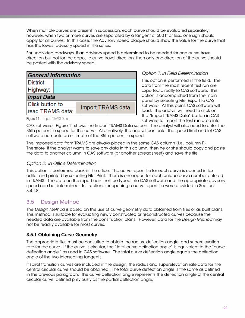
This option is performed in the field. The data from the most recent test run are exported directly to CAS software. This action is accomplished from the main panel by selecting File, Export to CAS software. At this point, CAS software will load. The analyst will need to click on the “Import TRAMS Data” button in CAS software to import the test run data into

CAS software. Figure 11 shows the Import TRAMS Data screen. The analyst will also need to enter the 85th percentile speed for the curve. Alternatively, the analyst can enter the speed limit and let CAS software compute an estimate of the 85th percentile speed.

The imported data from TRAMS are always placed in the same CAS column (i.e., column F). Therefore, if the analyst wants to save any data in this column, then he or she should copy and paste the data to another column in CAS software (or another spreadsheet) and save the file.

Option 2: In Office Determination

This option is performed back in the office. The curve report file for each curve is opened in text editor and printed by selecting File, Print. There is one report for each unique curve number entered in TRAMS. The data on the report can then be typed into CAS software and the appropriate advisory speed can be determined. Instructions for opening a curve report file were provided in Section 3.4.1.8.

3.5 Design MethodThe Design Method is based on the use of curve geometry data obtained from files or as built plans. This method is suitable for evaluating newly constructed or reconstructed curves because the needed data are available from the construction plans. However, data for the Design Method may not be readily available for most curves.

3.5.1 Obtaining Curve Geometry

The appropriate files must be consulted to obtain the radius, deflection angle, and superelevation rate for the curve. If the curve is circular, the “total curve deflection angle” is equivalent to the “curve deflection angle,” as used in CAS software. The total curve deflection angle equals the deflection angle of the two intersecting tangents.

If spiral transition curves are included in the design, the radius and superelevation rate data for the central circular curve should be obtained. The total curve deflection angle is the same as defined in the previous paragraph. The curve deflection angle represents the deflection angle of the central circular curve, defined previously as the partial deflection angle.

Figure 11 – Import TRAMS Data

23

If compound curvature is used in the design, the radius and superelevation rate data for the sharpest component curve should be obtained. The total curve deflection angle is the same as defined in the first paragraph. The curve deflection angle represents the deflection angle of the sharpest component curve.

If the road is divided or if conditions suggest the need for separate consideration of each curve travel direction, the aforementioned data for both directions of travel should be obtained. Although data for each curve should be obtained separately in this step, when two or more curves are separated by a tangent of 600 ft or less, one sign should apply for all curves.


The data obtained are entered in CAS software in the section titled Alternate Input Data. Note: the drop-down list at the top of the spreadsheet should be set to “Known curve geometry”. If a reasonable estimate of the 85th percentile tangent speed is not available, the speed limit can be used in CAS software to estimate the 85th percentile tangent speed.

Each curve should be evaluated separately in this step, but when two or more curves are separated by a tangent of 600 ft or less, one sign should apply for all curves. In this case, the Advisory Speed plaque should show the lowest advisory speed for the series of curves.


3.6 Ball-Bank Indicator MethodThe Ball-Bank Indicator Method is based on a set of field driving tests to record ball-bank indicator reading using a ball-bank indicator and a speedometer. There are varied criteria for establishing the curve advisory speed based on ball-bank indicator readings.

The AASHTO’s Geometric Design of Highways and Streets (2004) states that curve speeds that do not cause “driver discomfort” corresponding to ball-bank readings of 14-degree for speeds of 20 mph or less, 12-degree for speeds of 25 to 30 mph, and 10-degree for speeds of 35 mph or more. It notes that these readings are consistent with side friction factors of 0.21, 0.18, and 0.15, respectively.

The MUTCD 2003 edition indicates that the advisory speed may be the speed corresponding to a 16-degree ball-bank indicator reading. However, the MUTCD 2009 edition (3) modified the criteria as following:

•16 degrees of ball-bank for speeds of 20 mph or less,

•14 degrees of ball-bank for speeds of 25 to 30 mph, and

•12 degrees of ball-bank for speeds of 35 mph and higher.

The manual mentions that research has shown that drivers often exceed existing posted advisory curve speeds by 7 to 10 mph. The MUTCD 2009 edition (3) references posted advisory speeds determined by ball-bank values of 16, 14, and 12 degrees to address such driver behavior.

Ball-Bank Indicator Method determines the advisory speeds in the field using a vehicle equipped with a ball-bank indicator and an accurate speedometer. The speedometer should be check using a calibrated radar gun or other method. The simplicity of construction and operation of this device

24

has led to its widespread acceptance as a guide to determine advisory speeds for changes in horizontal alignment. Figure 12 shows a typical ball-bank indicator.

The ball-bank indicator consists of a curved glass tube which is filled with a liquid. A weighted ball floats in the glass tube. The ball-bank indicator is mounted in a vehicle, and as the vehicle travels around a curve, the ball floats outward in the curved glass tube. The movement of the ball is measured in

degrees of deflection, and this reading is indicative of the combined effect of superelevation, lateral (centripetal) acceleration, and vehicle body roll. The amount of body roll varies somewhat for different types of vehicles, and may affect the ball-bank reading by up to one degree, but generally is insignificant if a standard passenger car is used for the test. Therefore, when using this technique, it is best to use a typical passenger car rather than a pickup truck, van, or sports utility vehicle. Also, the ball-bank indicator test is normally a two-person operation, one person to drive and the other to record curve data and the ball-bank readings, especially if advisory speeds are being determined for a series of curves.

The Ball-Bank Indicator Method requires two people in the vehicle and multiple runs through the curve to get the correct advisory speed. In addition, reading the ball-bank indicator to determine the maximum degree of lean can be subjective.

3.6.1 Obtaining Field Measurements


To ensure proper results, it is critical that the following steps be taken before starting test runs with the ball-bank indicator:

• inflate all tires to uniform pressure as recommended by the vehicle manufacturer,

•calibrate the test vehicle’s speedometer, and

•zero the ball-bank indicator .

The vehicle speedometer is calibrated to ensure proper and consistent test results. This can be done by checking the vehicle speed with a radar or laser speed meter, or by timing the vehicle over a measured distance (such as milepost spacing). Alternatively, a moving radar unit can be used to measure speed while conducting the ball-bank test runs rather than relying on the vehicle’s speedometer.

The ball-bank indicator must be mounted in the vehicle so that it displays a 0-degree reading when the vehicle is stopped on a level surface. The positioning of the ball-bank indicator is checked before starting any test. This can be done by stopping the car so that its wheels straddle the centerline of a two-lane highway on a tangent alignment. In this position, the vehicle is essentially level, and the ball-bank indicator gives a reading of 0-degree. It is essential that the driver and recorder be in the same position in the vehicle when the ball-bank indicator is set to a 0-degree reading as they will be when the test runs are made because a shift in the load in the vehicle can affect the ball-bank indicator reading.

Figure 12 – Ball-Bank Indicator

25


Starting with a relatively low speed, the vehicle is driven through the curve at a constant speed following the curve alignment as closely as possible, and the reading on the ball-bank indicator is noted. On each test run, the driver must reach the test speed at a distance of at least ¼ mile in advance of the beginning of the curve, and maintain the same speed throughout the length of the curve. The path of the car must be maintained as nearly as possible in the center of the innermost lane (the lane closest to the inside edge of the curve) in the direction of travel. If there is more than one lane in the direction of travel, and these lanes have differing superelevation rates, the lane with the lowest amount of superelevation should be used. Because it is often difficult to drive the exact radius of the curve and keep the vehicle at a constant speed, it is suggested that at least three test runs in each direction be made to more accurately determine the ball-bank reading for any given speed. On each test run, the recorder carefully observes the position of the ball throughout the length of the curve and records the deflection reading that occurs when the vehicle is as nearly as possible driving the exact radius of the curve.

If the reading on the ball-bank indicator for a test run does not exceed the criteria stated in the MUTCD 2009 edition (3) (see Section 3.6, above), then the speed of the vehicle is increased by 5 mph and the test is repeated. The vehicle speed is repeatedly increased in 5 mph increments until the ball-bank indicator reading exceeds the acceptable maximum.


The curve advisory speed is set at the highest test speed that does not result in a ball-bank indicator reading greater than an acceptable level.

For example, a series of test runs for a curve were started at 25 mph, with ball-bank indicator reading of about 6-degree. This is well below the suggested criteria of 14-degree for a speed of 25 mph. The speeds of the test runs were increased in five mile an hour increments until the speed of 35 mph gave readings of 10-degree to 12-degree. These are the highest readings attained without exceeding the suggested criteria of 12-degree for a speed of 35 mph or more, because the speed of 40 mph gave the readings of 13-degree to 15-degree. Therefore, this field measurement would result in posting an advisory speed of 35 mph for this curve.

3.7 Accelerometer MethodAn accelerometer is an electronic device which can measure the lateral (centripetal) acceleration experienced by a vehicle as it travels around a curve. The Accelerometer Method can be used as an alternative to the Ball-Bank Indicator Method to establish the advisory speed (AASHTO’s 2004 Green Book (12), and MUTCD 2009 edition (3)).

The accelerometer is mounted on a level surface in a standard passenger vehicle such as on the windshield or along the floor centerline. An example of a commercially available unit is CurveRite 1200 shown in Figure 13. The CurveRite unit is equipped with a high-grade accelerometer and GPS that measures the lateral gravitational force that the vehicle encounters and the speed in which the average maximum lateral gravitational force was encountered.

Figure 13 – CurveRite Front Panel

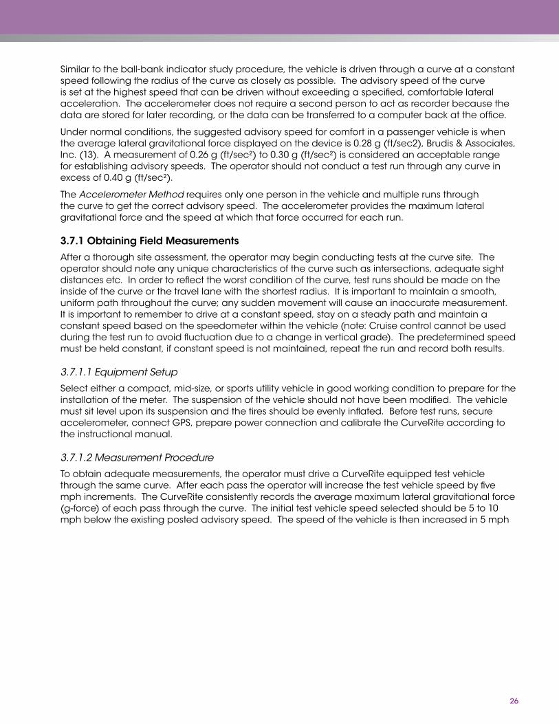
26

Similar to the ball-bank indicator study procedure, the vehicle is driven through a curve at a constant speed following the radius of the curve as closely as possible. The advisory speed of the curve is set at the highest speed that can be driven without exceeding a specified, comfortable lateral acceleration. The accelerometer does not require a second person to act as recorder because the data are stored for later recording, or the data can be transferred to a computer back at the office.

Under normal conditions, the suggested advisory speed for comfort in a passenger vehicle is when the average lateral gravitational force displayed on the device is 0.28 g (ft/sec2), Brudis & Associates, Inc. (13). A measurement of 0.26 g (ft/sec²) to 0.30 g (ft/sec²) is considered an acceptable range for establishing advisory speeds. The operator should not conduct a test run through any curve in excess of 0.40 g (ft/sec²).

The Accelerometer Method requires only one person in the vehicle and multiple runs through the curve to get the correct advisory speed. The accelerometer provides the maximum lateral gravitational force and the speed at which that force occurred for each run.

3.7.1 Obtaining Field Measurements

After a thorough site assessment, the operator may begin conducting tests at the curve site. The operator should note any unique characteristics of the curve such as intersections, adequate sight distances etc. In order to reflect the worst condition of the curve, test runs should be made on the inside of the curve or the travel lane with the shortest radius. It is important to maintain a smooth, uniform path throughout the curve; any sudden movement will cause an inaccurate measurement. It is important to remember to drive at a constant speed, stay on a steady path and maintain a constant speed based on the speedometer within the vehicle (note: Cruise control cannot be used during the test run to avoid fluctuation due to a change in vertical grade). The predetermined speed must be held constant, if constant speed is not maintained, repeat the run and record both results.


Select either a compact, mid-size, or sports utility vehicle in good working condition to prepare for the installation of the meter. The suspension of the vehicle should not have been modified. The vehicle must sit level upon its suspension and the tires should be evenly inflated. Before test runs, secure accelerometer, connect GPS, prepare power connection and calibrate the CurveRite according to the instructional manual.


To obtain adequate measurements, the operator must drive a CurveRite equipped test vehicle through the same curve. After each pass the operator will increase the test vehicle speed by five mph increments. The CurveRite consistently records the average maximum lateral gravitational force (g-force) of each pass through the curve. The initial test vehicle speed selected should be 5 to 10 mph below the existing posted advisory speed. The speed of the vehicle is then increased in 5 mph

27

increments in order to obtain a lateral g-force measurement above the recommended value of 0.28 g. The vehicle operator should stop increasing curve speeds when the test measurements exceed 0.40 g. Test runs should be conducted by following the steps:

•Start from a location ahead of the curve site to allow acceleration to determined test speed before beginning to turn through the curve (see Figure 14).

» Push the START button just before entering the curve at its tangent.

− The display will show “logging data” after pressing start.

» Push the STOP button after exiting the curve at its tangents.

− All data recording will then stop and the display will show “processing data”.

» The average maximum lateral g-force of the curve will then be displayed.

•The operator should proceed to a safe stopping location to record the results of the previous test run.

•Record CurveRite reading.

•After each run of the same curve (with the vehicle stopped), the operator must push the CLR button to reset the CurveRite meter.

•Pushing the CLR button does not remove the accelerometer calibration or vehicle classifications from memory.

•Repeat test run at 5 mph increments.


The curve advisory speed is set at the highest test speed that does not result in CurveRite reading greater than 0.28 g (ft/sec²).

For example, a series of test runs for a curve were started at 25 mph, then 30 mph, 35 mph, and 40 mph, with CurveRite reading of 0.22 g, 0.26 g, 0.28 g, and 0.29 g, respectively. 35 mph is the highest testing speed without exceeding the suggested criteria of 0.28 g. Therefore, this field measurement would result in posting an advisory speed of 35 mph for this curve.

StopTangent

Tangent

CurveTest Site

Start

Figure 14 – CurveRite Measurement

28

3.8 Confirming Speed for ConditionsThis procedure is to evaluate the appropriateness of the advisory speed determined. The field evaluation of curve conditions includes consideration of the following factors:

•approach sight distance at the beginning of the curve,

•visibility around the curve,

•unexpected geometric features within the curve, and

•position of the most critical curve in a sequence of closely spaced curves.

The unexpected geometric features noted in the third bullet may include:

•presence of an intersection,

•presence of a sharp crest vertical curve in the middle of the horizontal curve,

•sharp curves with changing radius (including curves with spiral transitions),

•sharp curves after a long tangent section, and

•broken-back curves.

A test run shall be conducted through the curve while traveling at the advisory speed determined in the previous description for each method. The engineer may choose to adjust the advisory speed or modify the warning sign layout based on consideration of the aforementioned factors.


3.9 Workshops and WebinarsA series of four workshops and one webinar were held across the country on establishing advisory curve speeds. The workshops were held in Maine, Virginia, Illinois and California. Discussions and comments that came up during the workshops included the following:

•Most attendees did not think that the existing advisory speeds are set at the correct speed.

•Several attendees felt that the advisory speed should be based on truck speed or should have a dual posting.

•Several attendees use the 85th percentile speed to determine the advisory speed.

•Most attendees do not think that advisory speeds should be set conservatively low. However, some attendees did think they should be conservatively low due to liability.

•Most, if not all, attendees would not use the Compass Method to determine the advisory speed. This is mostly due to the fact that this method requires that a vehicle must stop in the middle of the road to record data.

•Some attendees would use the GPS or Accelerometer Method except they lack the equipment.

•Most attendees use a ball-bank indicator or the electronic ball-bank indicator. Some use the Geometric Design Method or the 85th Percentile Speed Method.

•Most attendees like the Curve Advisory Speed Worksheet which would allow for consistent advisory speeds.

29

•Some attendees were concerned about how too many requirements translate into liability.

•During the presentation it was pointed out that the reverse curve sign was curving to the left and should be curving to the right (Slide 50). However, the MUTCD 2009 edition (3) says it is the direction of the first curve on the sign and the first curve on the road. This was agreed to, and it was also pointed out that if it is confusing to traffic engineers, it is probably confusing to the general public.

3.10 SummaryIn this chapter, the six (6) methods for establishing advisory curve speeds were introduced; and methodological procedures, including required equipment, software, installation and setup, and testing steps in the field were described. All methods can be used with the Curve Advisory Speed (CAS) software. The advisory speed is then determined based on the field measurements or known information and adjusted based on field confirmation and judgment.

The Direct Method is based on the field measurement of curve speeds under free-flow conditions. The devices used to record speeds are usually a radar speed meter and/or a traffic counter/classifier, both of which are commonly available devices to most traffic agencies. However, the traffic agencies do not have unanimous agreement regarding how best to determine the advisory speed given the distribution of curve speed and vehicle classification. The disagreement involves whether to use 85th percentile, average, or median speeds, as well as whether to use speeds of passenger cars, trucks, or all vehicles. Setting advisory speeds at 85th percentile speeds has been an accepted and common practice in the past, while also supported by the MUTCD 2003 edition, but is no longer a preferred approach in the MUTCD 2009 edition (3). Bonneson et al. (5) recommended using average truck speeds to determine advisory speeds.

The Compass Method is based on a single-pass survey technique using a digital compass, distance measuring instrument and ball-bank indicator to estimate the curve radius and deflection angle. The GPS Method is also based on a single pass survey using a GPS receiver and software to compute curve radius and deflection angle. The Design Method is useful when the radius and deflection angle are available from as built plans. The three methods were based on the TTI proposed curve speed prediction model which correlates the curve speed with the curve geometry. An Excel spreadsheet program Curve Advisory Speed (CAS) software was developed by TTI and hereafter enhanced to provide a means to calculate advisory speeds given curve geometry. The default model in the program is setting advisory speeds at average truck speed. The parameters in the program can be customized to setting advisory speeds at 85th percentile speeds of trucks and/or passenger cars.

The Ball-Bank Indicator Method is based on field driving tests to record ball-bank indicator readings using a ball-bank indicator and a speedometer. The simplicity of construction and operation of this device has led to its widespread acceptance as a guide to determine advisory speeds for changes in horizontal alignment; however, there are varied criteria for establishing the curve advisory speed based on ball-bank indicator readings. The AASHTO Green Book 2004 (12) recommends setting advisory speeds based on 14-degree for speeds of 20 mph or less, 12-degree for speeds of 25 to 30 mph, and 10-degree for speeds of 35 mph or more. The MUTCD 2009 edition (3) recommends the criteria of 16-degree, 14-degree, and 12-degree for the same range of speeds as in the AASHTO’s. The manual mentions that research has shown that drivers often exceed existing posted advisory curve speeds by 7 to 10 mph. The MUTCD 2009 edition (3) references posted advisory speeds determined by ball-bank values of 16, 14, and 12 degrees to address such driver behavior.

The Accelerometer Method is based on field driving tests that measure average lateral gravitational force using an electronic accelerometer device and a speedometer. It is an alternative to the Ball-Bank Indicator Method that is used to establish the advisory speed. CurveRite is a currently commercially available unit that can collect the required measurements. Unlike the Ball-Bank

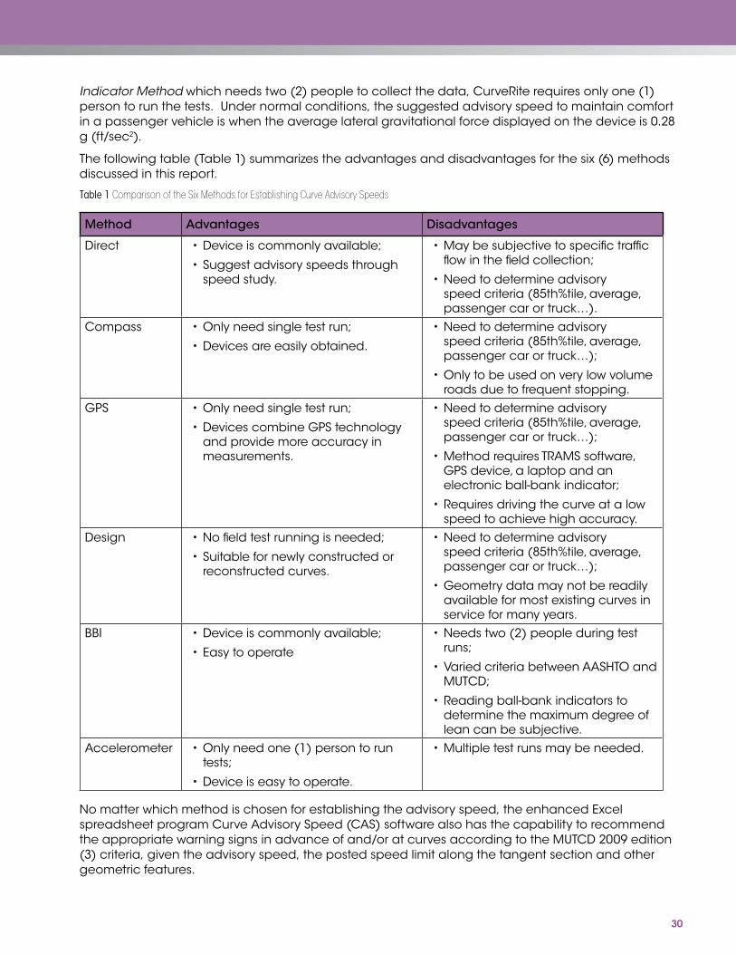
30

Indicator Method which needs two (2) people to collect the data, CurveRite requires only one (1) person to run the tests. Under normal conditions, the suggested advisory speed to maintain comfort in a passenger vehicle is when the average lateral gravitational force displayed on the device is 0.28 g (ft/sec2).

The following table (Table 1) summarizes the advantages and disadvantages for the six (6) methods discussed in this report.

Table 1 Comparison of the Six Methods for Establishing Curve Advisory Speeds

Method Advantages Disadvantages

Direct •Device is commonly available;

•Suggest advisory speeds through speed study.

•May be subjective to specific traffic flow in the field collection;

•Need to determine advisory speed criteria (85th%tile, average, passenger car or truck…).

Compass •Only need single test run;

•Devices are easily obtained.

•Need to determine advisory speed criteria (85th%tile, average, passenger car or truck…);

•Only to be used on very low volume roads due to frequent stopping.

GPS •Only need single test run;

•Devices combine GPS technology and provide more accuracy in measurements.


•Method requires TRAMS software, GPS device, a laptop and an electronic ball-bank indicator;

•Requires driving the curve at a low speed to achieve high accuracy.

Design •No field test running is needed;

•Suitable for newly constructed or reconstructed curves.


•Geometry data may not be readily available for most existing curves in service for many years.

BBI •Device is commonly available;

•Easy to operate

•Needs two (2) people during test runs;

•Varied criteria between AASHTO and MUTCD;

•Reading ball-bank indicators to determine the maximum degree of lean can be subjective.

Accelerometer •Only need one (1) person to run tests;

•Device is easy to operate.

•Multiple test runs may be needed.

No matter which method is chosen for establishing the advisory speed, the enhanced Excel spreadsheet program Curve Advisory Speed (CAS) software also has the capability to recommend the appropriate warning signs in advance of and/or at curves according to the MUTCD 2009 edition (3) criteria, given the advisory speed, the posted speed limit along the tangent section and other geometric features.

31

CHAPTer 4. CurVe SigNiNg guiDeliNeS

4.1 OverviewThis chapter describes guidelines for the signing of horizontal curves. These guidelines were derived from the MUTCD 2009 edition (3) and are intended to complement the procedures for establishing the advisory speed that are described in Chapter 3. Together, the procedure and guidelines provide a rational basis for establishing uniform signing for horizontal curves.

4.2 GuidelinesGuidelines for selecting curve related traffic control devices are described in this section and are based on the MUTCD 2009 edition (3). They consist of recommended combinations of traffic control devices associated with the difference between speed limits and advisory curve speeds. The guidelines were developed to reflect a balance of the following goals:

•Promote the uniform and consistent use of traffic control devices;

•Base guidance for these devices on difference between speed limit and advisory speed;

•Avoid overuse and misuse of devices; and

•Limit the number of devices used at a given curve.

A table in the MUTCD 2003 edition that related sign usage to the advisory speed and number of alignment changes has been replaced by a completely new table that relates sign usage to the difference between the speed limit and the advisory speed.

As shown in the Figure 15 of this report, the criteria in the MUTCD 2009 edition (3) states: “In advance of horizontal curves on freeways, on expressways, and on roadways with more than 1,000 AADT that are functionally classified as arterials or collectors, horizontal alignment warning signs shall be used in accordance with Table 2C-5 based on the speed differential between the roadway’s posted or statutory speed limit or 85th-percentile speed, whichever is higher, or the prevailing speed on the approach to the curve, and the horizontal curve’s advisory speed…Horizontal Alignment Warning signs may also be used on other roadways or on arterial and collector roadways with less than 1,000 AADT based on engineering judgment.”

Application of Table 2C-5. Horizontal Alignment Sign Selection (MUTCD 2009 edition (3)) (see Figure 15 of this report) requires knowledge of the 85th percentile tangent speed for passenger cars. This speed can be obtained from a survey of speeds on a tangent section of highway in the vicinity of the curve. The location at which tangent speed data are collected should be sufficiently distant from the curve that the curve does not influence the observed speeds. If the 85th percentile tangent speed is not available, an equation is provided in the Curve Advisory Speed (CAS) software for estimating this speed.

32

Table 2C-5. Horizontal Alignment Sign Selection

Type of Horizontal Alignment Sign

Difference Between Speed Limit and Advisory Speed

5 mph 10 mph 15 mph 20 mph 25 mph or more

Turn (W1-1), Curve (W1-2), Reverse Turn (W1-3), Reverse Curve (W1-4), Winding Road (W1-5), and Combination Horizontal Alignment/Intersection (W10-1) (see Section 2C.07 to determine which sign to use)

Recommended Required Required Required Required

Advisory Speed Plaque (W13-1P) Recommended Required Required Required Required

Chevrons (W1-8) and/or One Direction Large Arrow (W1-6) Optional Recommended Required Required Required

Exit Speed (W13-2) and Ramp Speed (W13-3) on exit ramp

Optional Optional Recommended Required Required

Note: Required means that the sign and/or plaque shall be used, recommended means that the sign and/or plaque should be used, and optional means that the sign and/or plaque may be used.

See Section 2C.06 for roadways with less than 1,000 ADT.

Figure 15 – MUTCD 2009 Edition Criteria for the Selection of Horizontal Alignment Sign

There is a new table (see Figure 16) added to the MUTCD 2009 edition (3), “Table 2C-6. Typical Spacing of Chevron Alignment Signs on Horizontal Curves.”

Figure 16 – MUTCD 2009 Edition Criteria for the Typical Spacing of Chevron Alignment Signs on Horizontal Curves

To determine the location for installing advance horizontal alignment warning signs, “Table 2C-4. Guidelines for Advance Placement of Warning Signs” in the MUTCD 2009 edition (3) shall be consulted (Refer to Figure 17).

Table 2C-6. Typical Spacing of Chevron Alignment Signs on Horizontal Curves

Advisory Speed

15 mph or less

20 to 30 mph

35 to 45 mph

50 to 60 mph

More than 60 mph

Note: The relationship between the curve radius and the advisory speed shown in this table should not be used to determine the advisory speed.

Sign Spacing

40 feet

80 feet

120 feet

160 feet

200 feet

Curve Radius

Less than 200 feet

200 to 400 feet

401 to 700 feet

701 to 1,250 feet

More than 1,250 feet

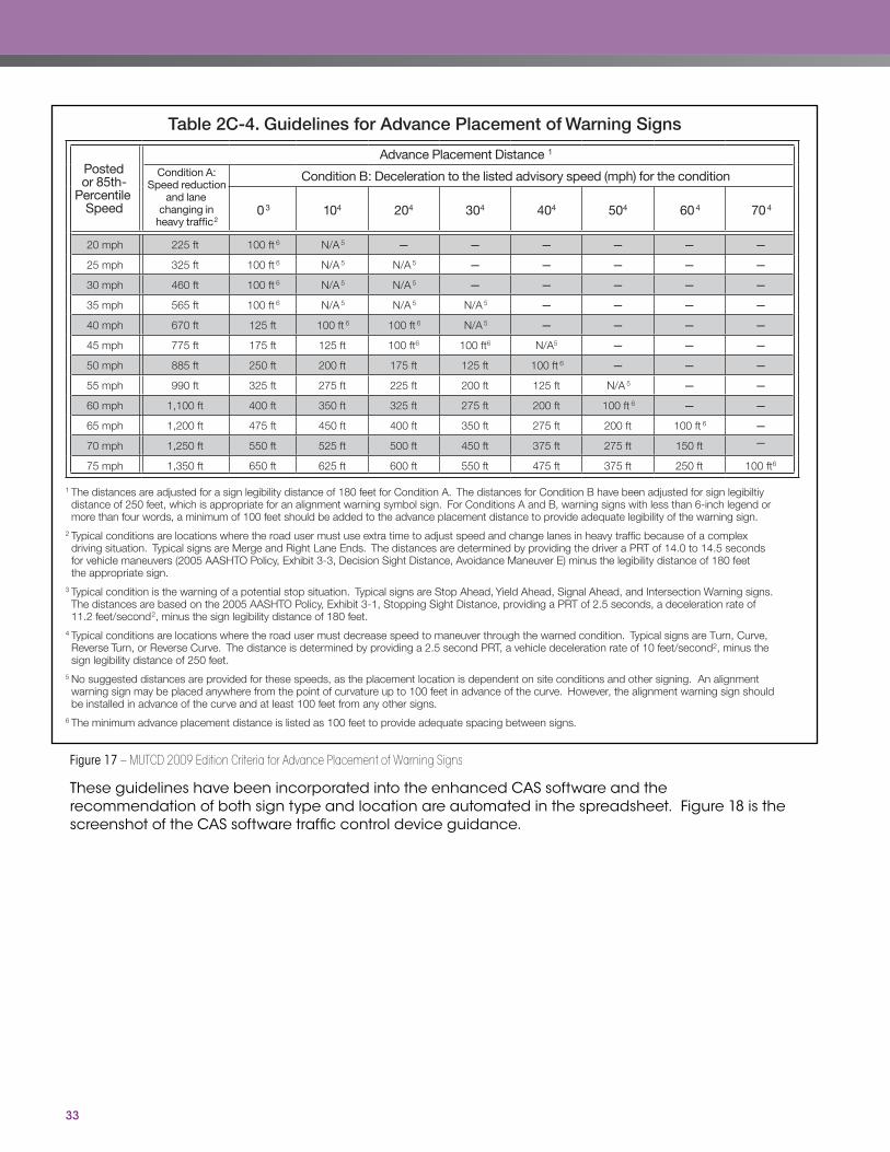
33

Figure 17 – MUTCD 2009 Edition Criteria for Advance Placement of Warning Signs

These guidelines have been incorporated into the enhanced CAS software and the recommendation of both sign type and location are automated in the spreadsheet. Figure 18 is the screenshot of the CAS software traffic control device guidance.

Table 2C-4. Guidelines for Advance Placement of Warning Signs

Posted or 85th-

Percentile Speed

Advance Placement Distance 1

Condition A: Speed reduction

and lane changing in

heavy traffic2

Condition B: Deceleration to the listed advisory speed (mph) for the condition

03 104 204 304 404 504 604 704

20 mph 225 ft 100 ft 6 N/A 5

25 mph 325 ft 100 ft 6 N/A 5 N/A 5

30 mph 460 ft 100 ft 6 N/A 5 N/A 5

35 mph 565 ft 100 ft 6 N/A 5 N/A 5 N/A 5

40 mph 670 ft 125 ft 100 ft 6 100 ft 6 N/A 5

45 mph 775 ft 175 ft 125 ft 100 ft6 100 ft6 N/A5

50 mph 885 ft 250 ft 200 ft 175 ft 125 ft 100 ft 6

55 mph 990 ft 325 ft 275 ft 225 ft 200 ft 125 ft N/A 5

60 mph 1,100 ft 400 ft 350 ft 325 ft 275 ft 200 ft 100 ft 6

65 mph 1,200 ft 475 ft 450 ft 400 ft 350 ft 275 ft 200 ft 100 ft 6

— — — — — —

— — — — —

— — — — —

— — — —

— — — —

— — —

— — —

— —

— —

—

—70 mph 1,250 ft 550 ft 525 ft 500 ft 450 ft 375 ft 275 ft 150 ft

75 mph 1,350 ft 650 ft 625 ft 600 ft 550 ft 475 ft 375 ft 250 ft 100 ft6

1 The distances are adjusted for a sign legibility distance of 180 feet for Condition A. The distances for Condition B have been adjusted for sign legibiltiydistance of 250 feet, which is appropriate for an alignment warning symbol sign. For Conditions A and B, warning signs with less than 6-inch legend ormore than four words, a minimum of 100 feet should be added to the advance placement distance to provide adequate legibility of the warning sign.

2 Typical conditions are locations where the road user must use extra time to adjust speed and change lanes in heavy traffic because of a complexdriving situation. Typical signs are Merge and Right Lane Ends. The distances are determined by providing the driver a PRT of 14.0 to 14.5 secondsfor vehicle maneuvers (2005 AASHTO Policy, Exhibit 3-3, Decision Sight Distance, Avoidance Maneuver E) minus the legibility distance of 180 feetthe appropriate sign.

3 Typical condition is the warning of a potential stop situation. Typical signs are Stop Ahead, Yield Ahead, Signal Ahead, and Intersection Warning signs. The distances are based on the 2005 AASHTO Policy, Exhibit 3-1, Stopping Sight Distance, providing a PRT of 2.5 seconds, a deceleration rate of11.2 feet/second2, minus the sign legibility distance of 180 feet.

4 Typical conditions are locations where the road user must decrease speed to maneuver through the warned condition. Typical signs are Turn, Curve,Reverse Turn, or Reverse Curve. The distance is determined by providing a 2.5 second PRT, a vehicle deceleration rate of 10 feet/second2, minus thesign legibility distance of 250 feet.

5 No suggested distances are provided for these speeds, as the placement location is dependent on site conditions and other signing. An alignmentwarning sign may be placed anywhere from the point of curvature up to 100 feet in advance of the curve. However, the alignment warning sign shouldbe installed in advance of the curve and at least 100 feet from any other signs.

6 The minimum advance placement distance is listed as 100 feet to provide adequate spacing between signs.

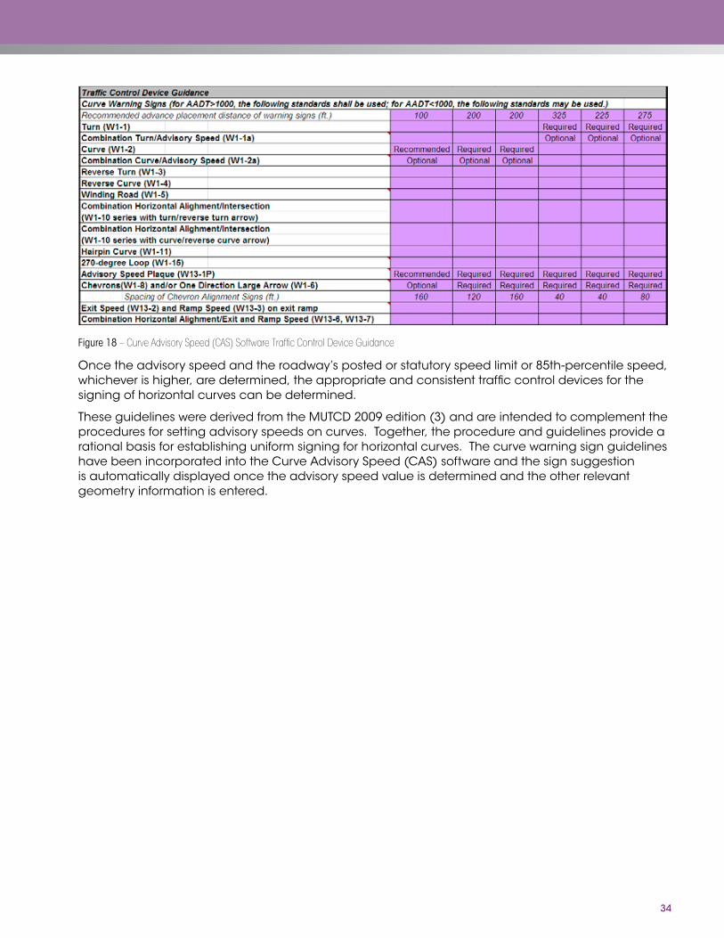
34

Figure 18 – Curve Advisory Speed (CAS) Software Traffic Control Device Guidance

Once the advisory speed and the roadway’s posted or statutory speed limit or 85th-percentile speed, whichever is higher, are determined, the appropriate and consistent traffic control devices for the signing of horizontal curves can be determined.

These guidelines were derived from the MUTCD 2009 edition (3) and are intended to complement the procedures for setting advisory speeds on curves. Together, the procedure and guidelines provide a rational basis for establishing uniform signing for horizontal curves. The curve warning sign guidelines have been incorporated into the Curve Advisory Speed (CAS) software and the sign suggestion is automatically displayed once the advisory speed value is determined and the other relevant geometry information is entered.

35

refereNCeS1. Bonneson, J, M. Pratt, J. Miles, and P. Carlson. “Procedures for Setting Curve Advisory Speeds.” FHWA/TX-09/5-5439-

01-P1. Federal Highway Administration, U.S. Department of Transportation, Washington, D.C., and Texas Department of Transportation, Austin, Texas, 2009.

2. Torbic, D.J., D.W. Harwood, D.K. Gilmore, R. Pfefer, T.R. Neuman, K.L. Slack, and K.K. Hardy. “NCHRP Report 500: Guidance for Implemention of the AASHTO Strategic Highway Safety Plan - Volume 7: A Guide for Reducing Collisions on Horizontal Curves”. Transportation Research Board, Washington, D.C., 2004.

3. Manual on Uniform Traffic Control Devices. Federal Highway Administration, U.S. Department of Transportation, Washington, D.C., 2009.

4. Chowdhury, M., D. Warren, H. Bissell, and S. Taori. “Are the Criteria for Setting Advisory Speeds on Curves Still Relevant?” ITE Journal. Institute of Transportation Engineers, Washington, D.C., February 1998, pp. 32-45.

5. Bonneson, J, M. Pratt, J. Miles, and P. Carlson. “Development of Guidelines for Establishing Effective Curve Advisory Speeds”. FHWA/TX-07/0-5439 1. Texas Department of Transportation, Austin, Texas, 2007.

6. Bonneson, J., D. Lord, K. Zimmerman, K. Fitzpatrick, and M. Pratt. “Development of Tools for Evaluating the Safety Implications of Highway Design Decisions”. FHWA/TX-07/0-4703 4. Texas Department of Transportation, Austin, Texas, September 2006.

7. Fitzpatrick, K., L. Elefteriadou, D.W. Harwood, J.M. Collins, J. McFadden, I.B. Anderson, R.A. Krammes, N. Irizarry, K.D. Parma, K.M. Bauer, and K. Passetti. “Speed Prediction for Two-Lane Rural Highways”. FHWA-RD-99-171. Federal Highway Administration, U.S. Department of Transportation, 2000.

8. Manual on Uniform Traffic Control Devices. Federal Highway Administration, U.S. Department of Transportation, Washington, D.C., 2003.

9. Pietrucha, M.T., K.S. Opiela, R.L. Knoblauch, and K.L. Crigler. “Motorist Compliance with Standard Traffic Control Devices”. FHWA-RD-89-103. Federal Highway Administration, U.S. Department of Transportation, Washington, D.C., 1989.

10. Hammer, Jr., C.G. “Evaluation of Minor Improvements: Part 6, Signs”. California Division of Highways, Traffic Department, May 1968.

11. Ritchie, M.L. “A Choice of Speed in Driving through Curves as a Function of Advisory Speed and Curve Signs.” Human Factors. Vol. 14, No. 6. December 1972.

12. American Association of State Highway and Transportation Officials (AASHTO), “A Policy on Geometric Design of Highways and Streets”, 5th Edition, 2004.

13. Brudis & Associates, Inc., Advisory Speeds on Maryland Highways, Technical Report for Maryland DOT, August 1999.

For More Information:

http://website.com

FHWA, Office of Safety

Guan [email protected]

FHWA-SA-11-22

http://safety.fhwa.dot.gov/ped_bike

mailto:guan.xu%40dot.gov?subject=

procedures for setting advisory speeds on curves · speed, engineering study methods for...

Documents