PROCESS-BASED,DISTRIBUTED

WATERSHED MODELS

•New generation•Source waters and flowpaths•Physically based

Objectives

• Use distributed hydrologic modeling to improve understanding of the – Hydrology (flowpaths?)– water balance – streamflow variability– contaminant transport

Objectives, continued

• Test and validate model components and complete model against internal and spatially distributed measurements.– Isotopes are often ideal for cross-validating

model results

Objectives, continued

• Evaluate the level of complexity needed to provide adequate characterization of streamflow at various scales.– Evaluate minimum data requirements– Evaluate minimum process-level information

Objectives, continued

• Quantify spatial heterogeneity of inputs (rainfall, topography, soils - where data exist) and relate this to heterogeneity in streamflow.

Objectives, continued

• Role of groundwater?

• Fracture flow?

• Back out as residual?

Top Ten Reasons for Modeling

• You don’t need data!

• You don’t need to conduct fieldwork!

• We’ll model it!

• Synthesis

• Diagnostic

• Prognostic

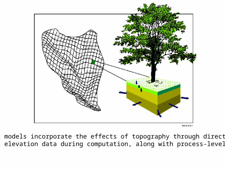
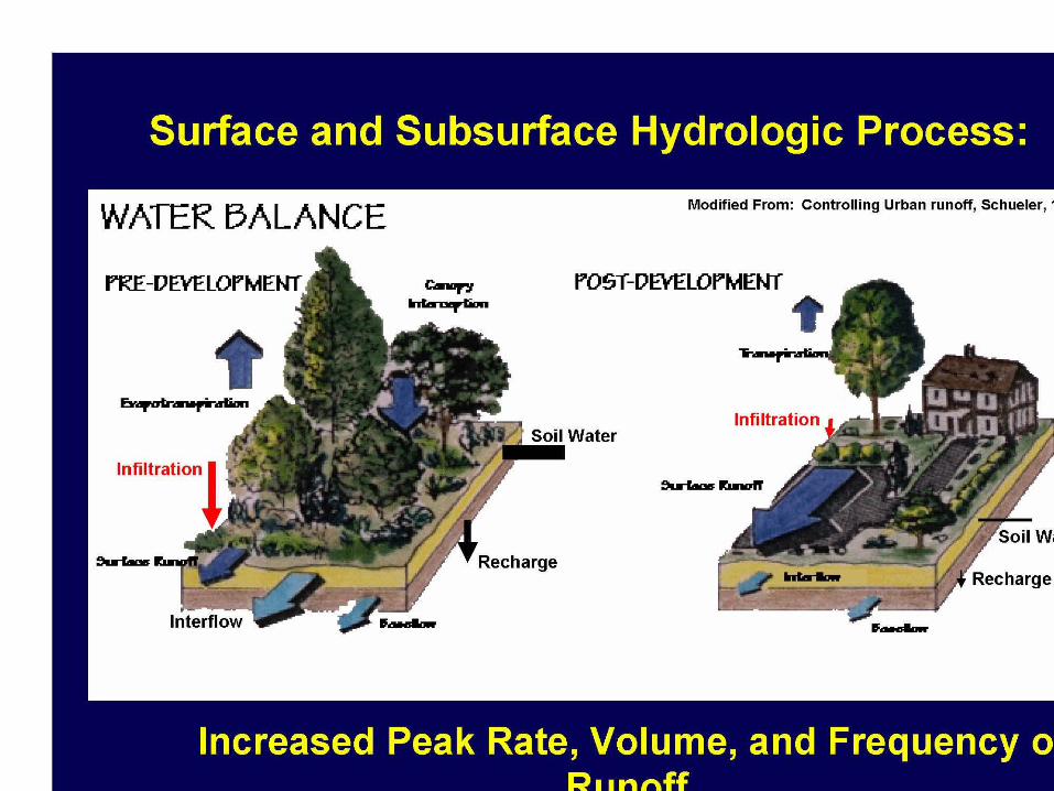
Distributed models incorporate the effects of topography through direct used of the digital elevation data during computation, along with process-level knowledge.

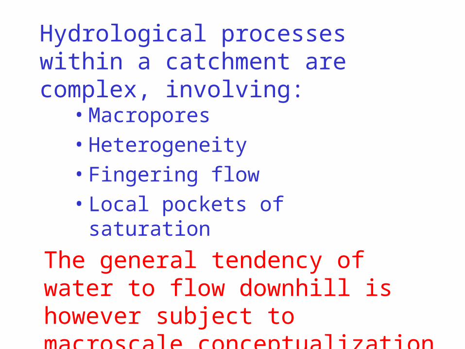
Hydrological processes within a catchment are complex, involving:

• Macropores

• Heterogeneity

• Fingering flow

• Local pockets of saturation

The general tendency of water to flow downhill is however subject to macroscale conceptualization

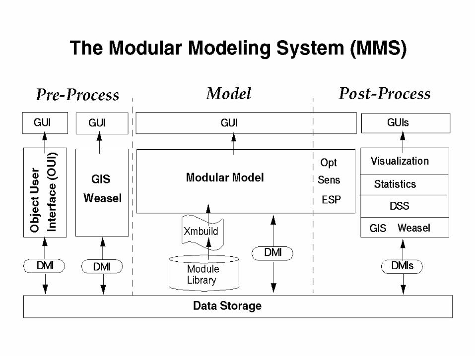
MMS Modular Modeling System

PRMS on Steroids• Conceptually, the framework is an integrated

system of computer software designed to provide the modeling tools needed to support a broad range of model applications and model user skills. The framework supports the

1. application and analysis of existing models, 2. modification and enhancement of existing models for

problem-specific applications, 3. research, devleopment, testing, and application of

new models.

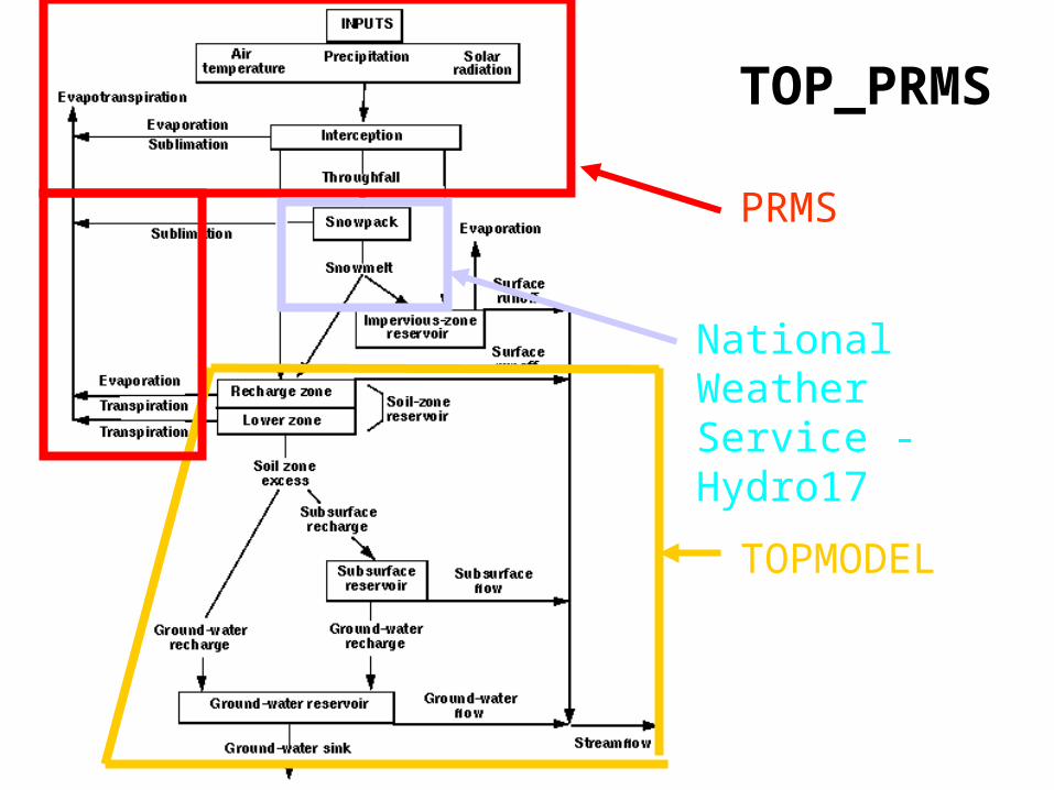
TOP_PRMS

PRMS

National Weather Service - Hydro17

TOPMODEL

PRECIPITATION-RUNOFF MODELING SYSTEM

(PRMS)

MODELING OVERVIEW

&

DAILY MODE COMPONENTS

http://wwwbrr.cr.usgs.gov/projects/SW_precip_runoff/

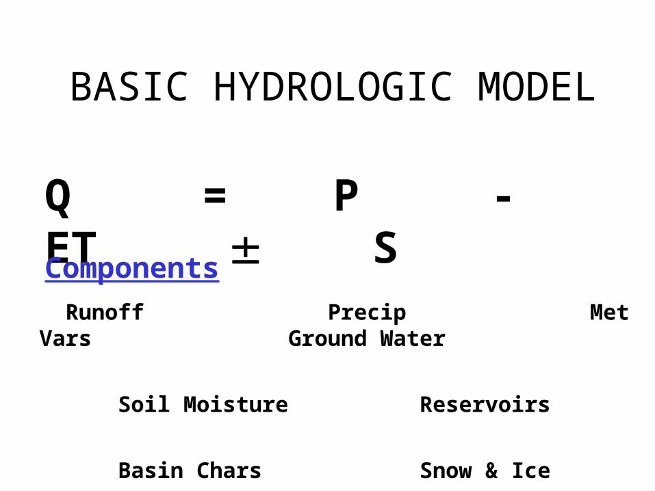
BASIC HYDROLOGIC MODEL

Q = P - ET S

Runoff Precip Met Vars Ground Water

Soil Moisture Reservoirs

Basin Chars Snow & Ice

Water use Soil Moisture

Components

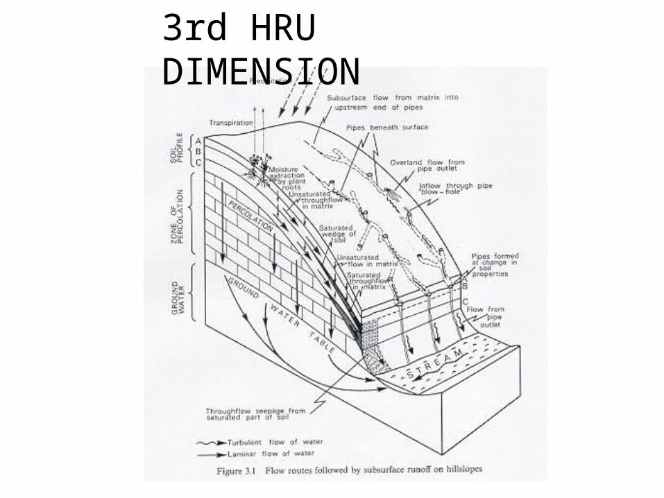
3rd HRU DIMENSION

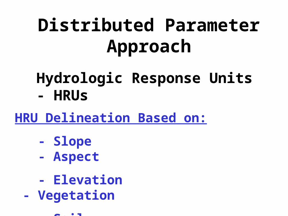
Distributed Parameter Approach

Hydrologic Response Units - HRUs

HRU Delineation Based on:

- Slope - Aspect

- Elevation - Vegetation

- Soil - Precip Distribution

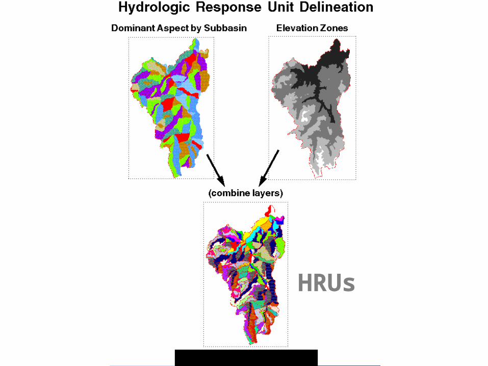
HRUs

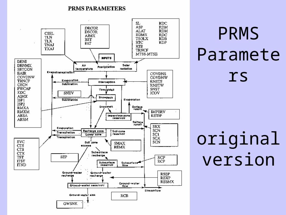
PRMS Parameters

original version

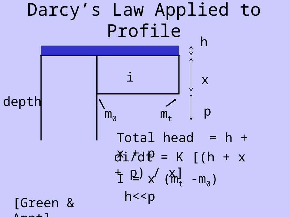
Darcy’s Law Applied to Profile

depth

h

x

p

Total head = h + x + p

di/dt = K [(h + x + p) / x]

i

I = x (mt -m0) h<<p

mtm0

[Green & Ampt]

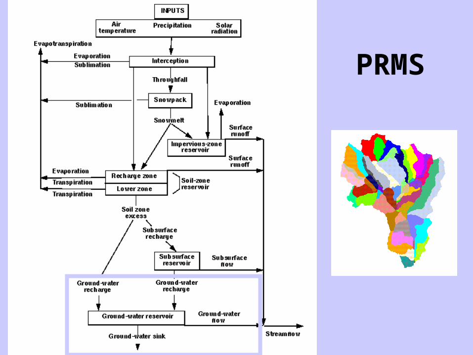
PRMS

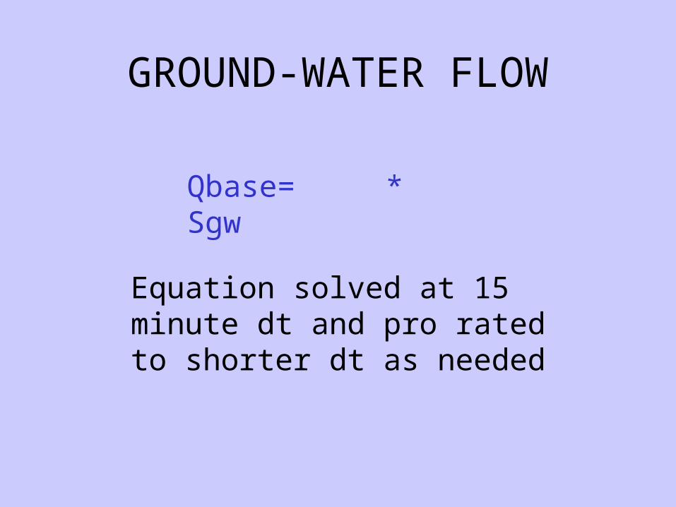
GROUND-WATER FLOW

Qbase= RCB * Sgw

Equation solved at 15 minute dt and pro rated to shorter dt as needed

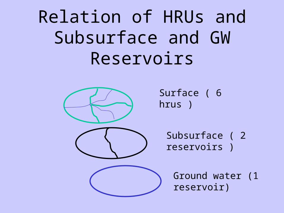
Relation of HRUs and Subsurface and GW Reservoirs

Surface ( 6 hrus )

Subsurface ( 2 reservoirs )

Ground water (1 reservoir)

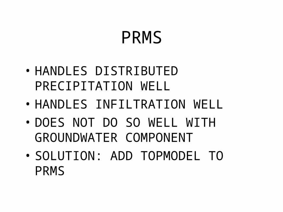
PRMS

• HANDLES DISTRIBUTED PRECIPITATION WELL

• HANDLES INFILTRATION WELL

• DOES NOT DO SO WELL WITH GROUNDWATER COMPONENT

• SOLUTION: ADD TOPMODEL TO PRMS

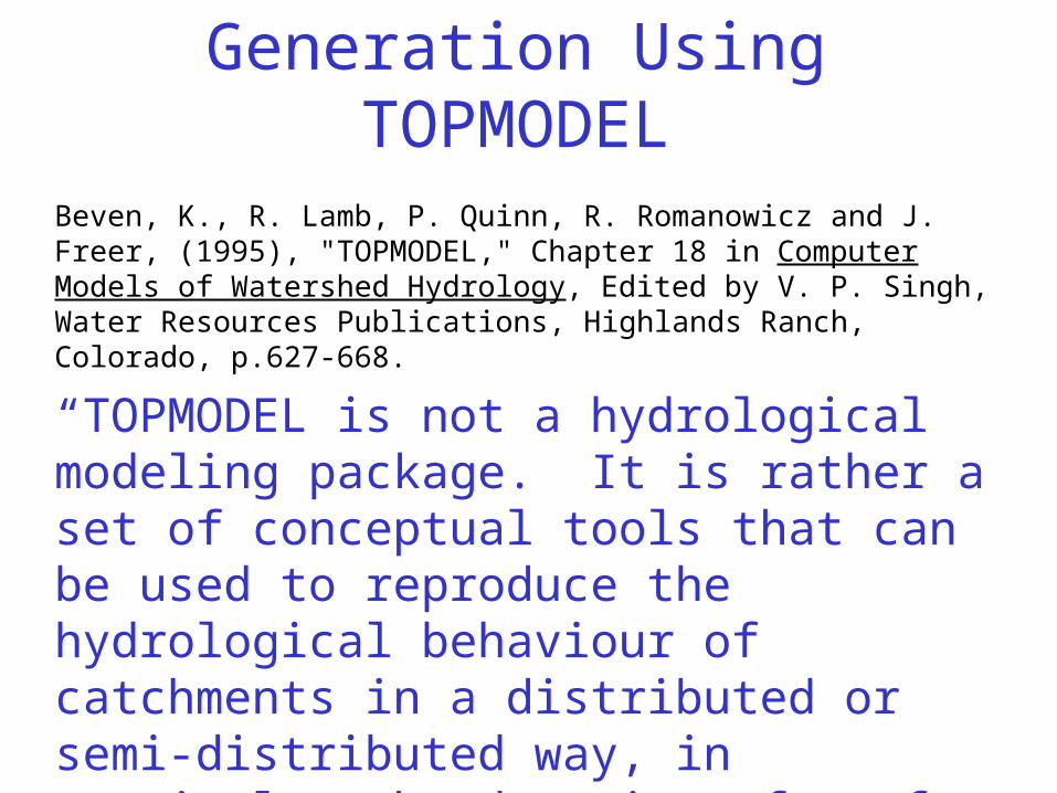
Terrain Based Runoff Generation Using TOPMODEL

Beven, K., R. Lamb, P. Quinn, R. Romanowicz and J. Freer, (1995), "TOPMODEL," Chapter 18 in Computer Models of Watershed Hydrology, Edited by V. P. Singh, Water Resources Publications, Highlands Ranch, Colorado, p.627-668.

“TOPMODEL is not a hydrological modeling package. It is rather a set of conceptual tools that can be used to reproduce the hydrological behaviour of catchments in a distributed or semi-distributed way, in particular the dynamics of surface or subsurface contributing areas.”

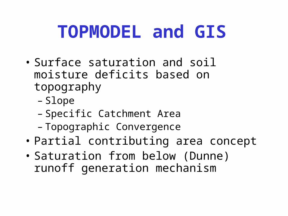
TOPMODEL and GIS

• Surface saturation and soil moisture deficits based on topography– Slope– Specific Catchment Area– Topographic Convergence

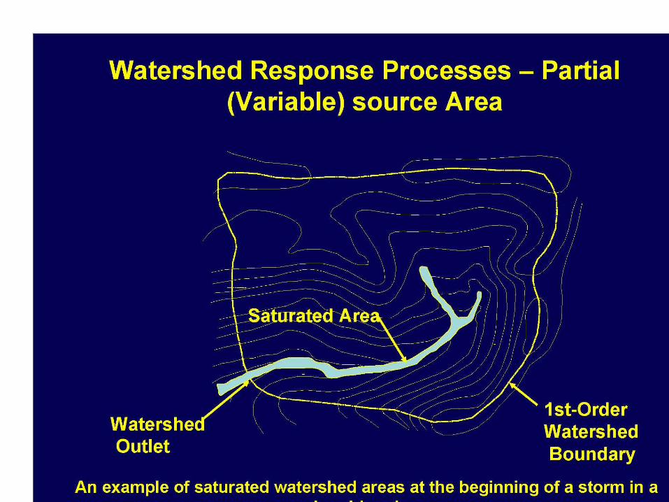
• Partial contributing area concept• Saturation from below (Dunne) runoff

generation mechanism

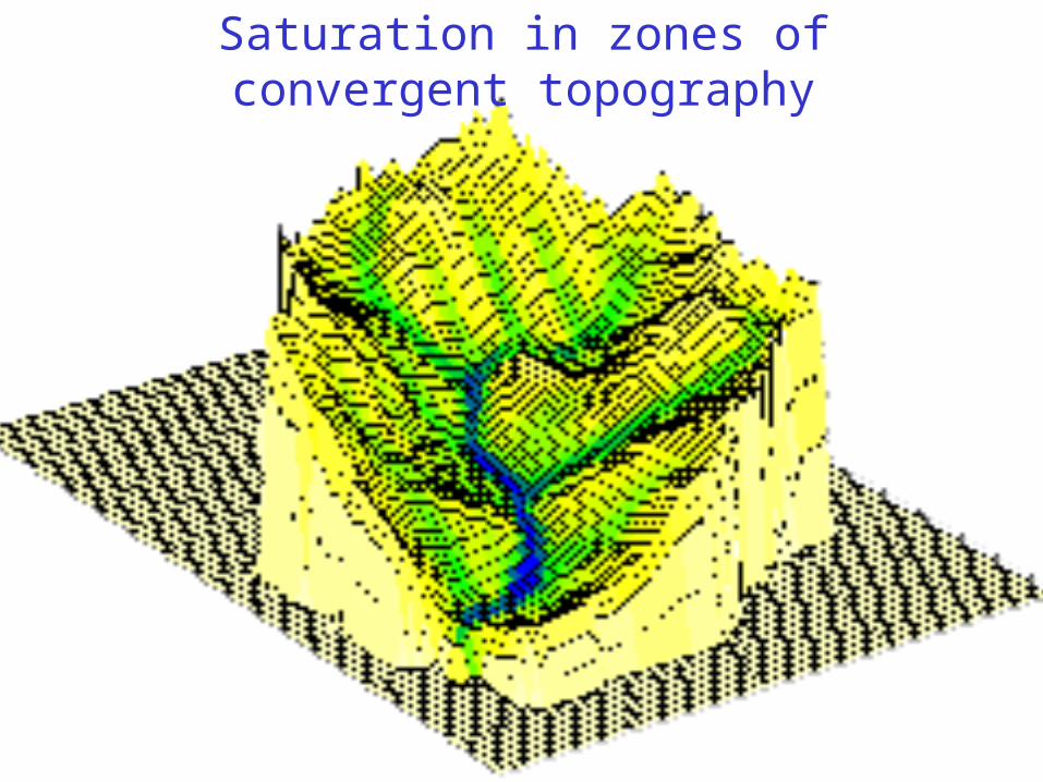
Saturation in zones of convergent topography

Topographic Index

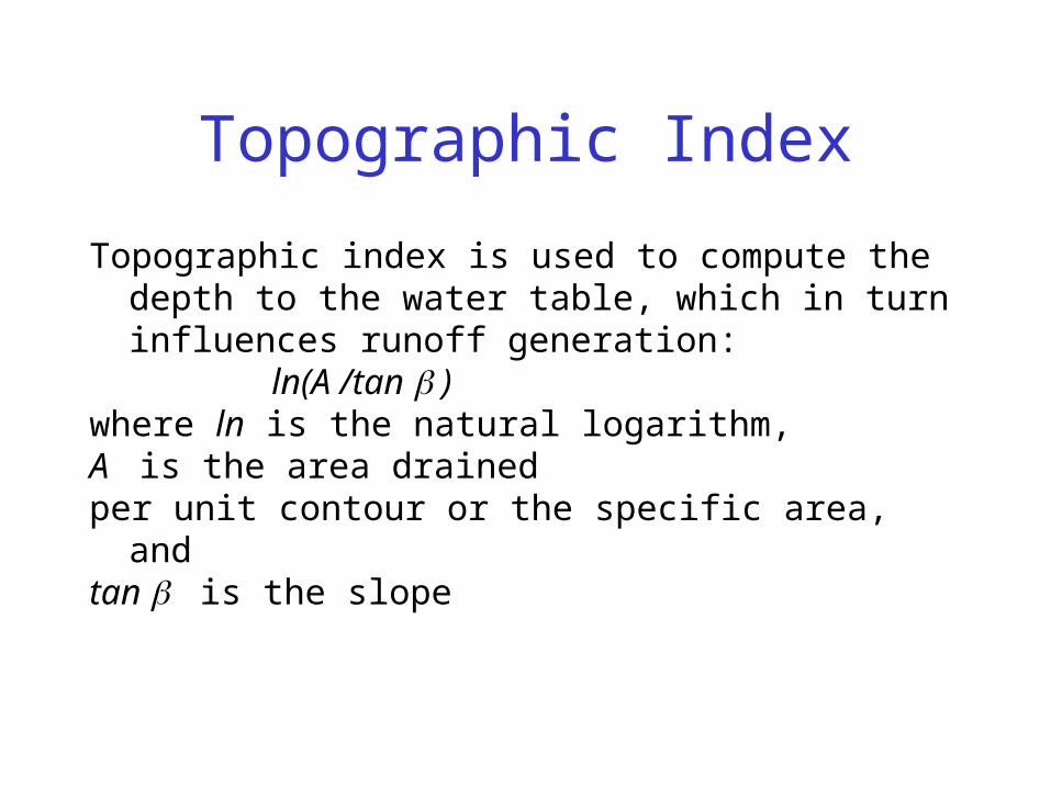
Topographic index is used to compute the depth to the water table, which in turn influences runoff generation:

ln(A /tan )where ln is the natural logarithm, A is the area drained per unit contour or the specific area, and tan is the slope

Topographic Index

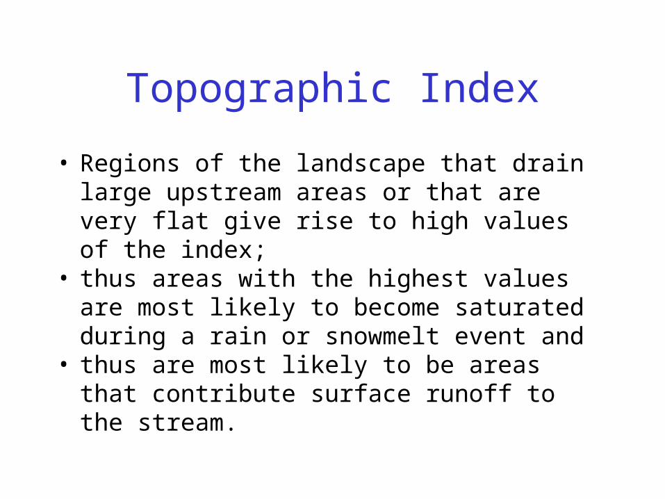
• Regions of the landscape that drain large upstream areas or that are very flat give rise to high values of the index;

• thus areas with the highest values are most likely to become saturated during a rain or snowmelt event and

• thus are most likely to be areas that contribute surface runoff to the stream.

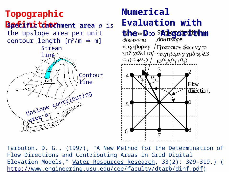
Flowdirection.

Steepest directiondownslope

α1

α2

1

234

5

67

8

Proportionflowingtoneighboringgridcell3isα2/(α1+α2)

Proportionflowingtoneighboringgridcell4isα1/(α1+α2)

Numerical Evaluation with the D Algorithm

Upslope contributing area a

Stream line

Contour line

Topographic DefinitionSpecific catchment area a is the upslope area per unit contour length [m2/m m]

Tarboton, D. G., (1997), "A New Method for the Determination of Flow Directions and Contributing Areas in Grid Digital Elevation Models," Water Resources Research, 33(2): 309-319.) (http://www.engineering.usu.edu/cee/faculty/dtarb/dinf.pdf)

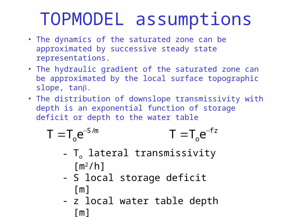
TOPMODEL assumptions• The dynamics of the saturated zone can be approximated

by successive steady state representations.

• The hydraulic gradient of the saturated zone can be approximated by the local surface topographic slope, tan.

• The distribution of downslope transmissivity with depth is an exponential function of storage deficit or depth to the water table

m/SoeTT −= fz

oeTT −=- To lateral transmissivity [m2/h]- S local storage deficit [m]- z local water table depth [m]- m a parameter [m]- f a scaling parameter [m-1]

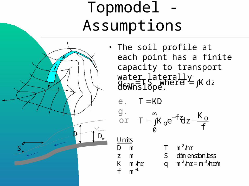
Topmodel - Assumptions

• The soil profile at each point has a finite capacity to transport water laterally downslope.

∫== dzKTwhereSTqcap

f

KdzeKT

KDT

o

0

fzo =∫=

=∞ −

e.g.

or

UnitsD mz mK m/hrf m-1

T m2/hrS dimensionlessq m2/hr = m3/hr/m

S

DwD

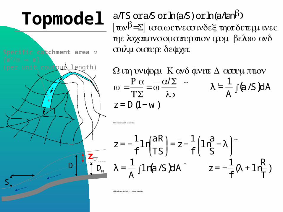
a/TS or a/S or ln(a/S) or ln(a/tan)[tαn=S]isαwetnessindexthαtdeterm inesthelocαtionsofsαturαtionfrom elowαndsoilm oisturedeficit.

W ithuniform KαndfiniteDαssum ption

'S/αw

STαRw

l==

where

( )∫=λ dAS/aA1

'

)w1(Dz −=

With exponential K assumption

⎟⎠⎞

⎜⎝⎛ λ−−=⎟

⎠⎞

⎜⎝⎛−=

Sa

lnf1

zTSaR

lnf1

z where

( )∫=λ dAS/alnA1 and

)TR

ln(f1

z +λ−=

Soil moisture deficit = z times porosity

Topmodel

Specific catchment area a [m2/m m] (per unit coutour length)

S

DwD

z

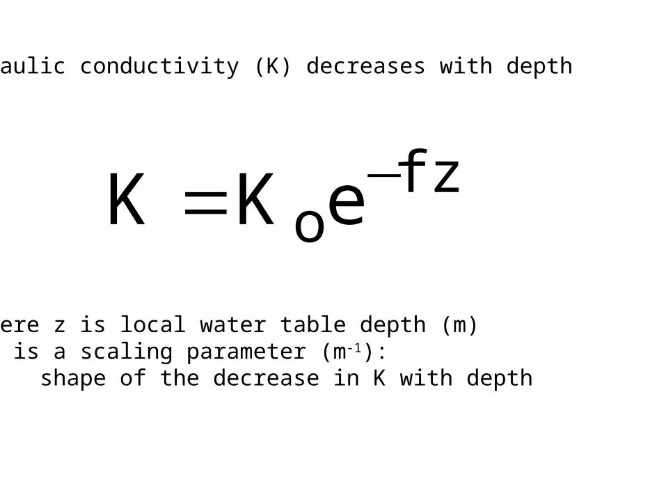
zfoeKK −=

Hydraulic conductivity (K) decreases with depth

where z is local water table depth (m) f is a scaling parameter (m-1):

shape of the decrease in K with depth

GL4 CASE STUDY: OBJECTIVES

• to test the applicability of the TOP_PRMS model for runoff simulation in seasonally snow-covered alpine catchments

• to understand flowpaths determined by the TOP_PRMS model

• to validate the flowpaths by comparing them with the flowpaths determined by tracer-mixing model

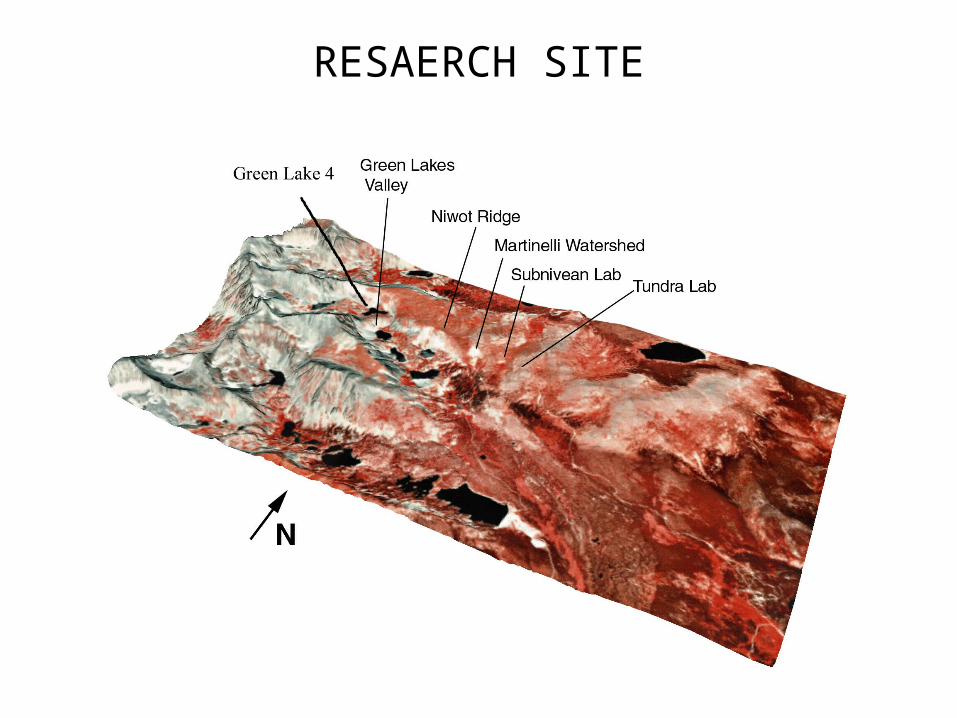
RESAERCH SITE

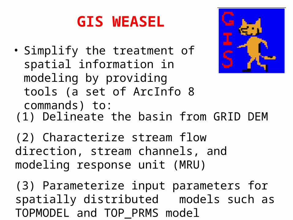
GIS WEASEL

• Simplify the treatment of spatial information in modeling by providing tools (a set of ArcInfo 8 commands) to:

(1) Delineate the basin from GRID DEM

(2) Characterize stream flow direction, stream channels, and modeling response unit (MRU)

(3) Parameterize input parameters for spatially distributed models such as TOPMODEL and TOP_PRMS model

PROCEDURES FOR DELINEATION AND PARAMETERIZATION

• DEM (10 m) was converted from TIN to GRID format using ArcInfo 8 commands

• a pour-point coverage was generated using location information of gauging stations

• DEM and the pour-point coverage were overlaid to delineate the basin

• DEM slope and direction were re-classified to extract the drainage network

• a base input parameter file and re-classified DEM were used to derive parameters needed for TOP_PRMS model

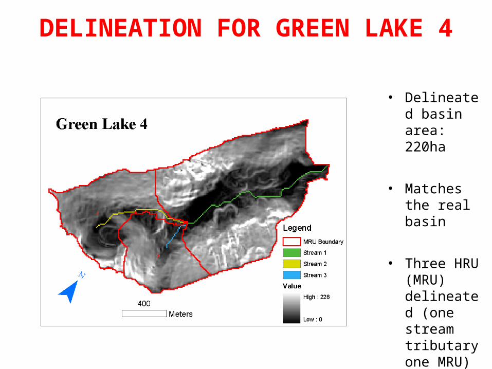
DELINEATION FOR GREEN LAKE 4

• Delineated basin area: 220ha

• Matches the real basin

• Three HRU (MRU) delineated (one stream tributary one MRU)

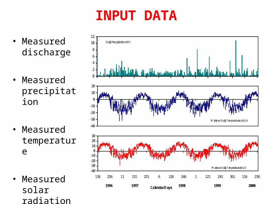
INPUT DATA

• Measured discharge

• Measured precipitation

• Measured temperature

• Measured solar radiation

Maximum Daily Temperature at GL4-40-30-20-10

0102030

136 256 11 131 251 6 126 246 1 121 241 361 116 236

Calendar Days

Temperature (

o C)

1997 1998 1999 20001996

Daily Precipitation at D1

0

2

4

6

8

10

12

Precipitation (cm)

Minimum Daily Temperature at GL4

-40

-30

-20

-10

0

10

20

Temperature (

oC)

Calibration

• Calibrate model with discharge in 1996

• Model calibrates internal processes and parameters to match discharge

• Run model with climate parameters from modeling years

• Calibration is key

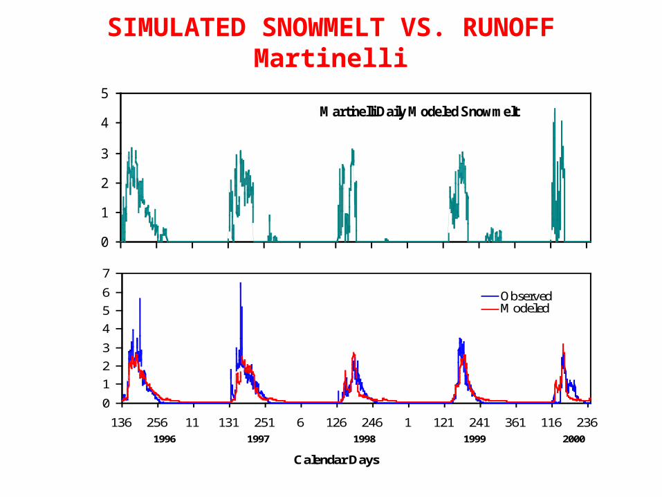
SIMULATED SNOWMELT VS. RUNOFFMartinelli

0

1

2

3

4

5

6

7

136 256 11 131 251 6 126 246 1 121 241 361 116 236

Calendar Days

Runoff (cm)

ObservedModeled

1997 1998 1999 20001996

Martinelli Daily Modeled Snowmelt

0

1

2

3

4

5

Snowmelt (cm)

Model Verification

• Discharge is almost always used

• Good idea or bad idea? Why?

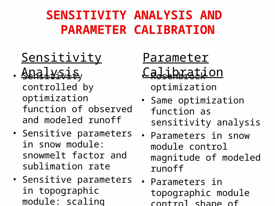
SENSITIVITY ANALYSIS AND PARAMETER CALIBRATION

• Sensitivity controlled by optimization function of observed and modeled runoff

• Sensitive parameters in snow module: snowmelt factor and sublimation rate

• Sensitive parameters in topographic module: scaling factor and transmissivity

• Rosenbrock optimization

• Same optimization function as sensitivity analysis

• Parameters in snow module control magnitude of modeled runoff

• Parameters in topographic module control shape of rising and receding limbs

• Improvement evaluated by modeling efficiency

Sensitivity Analysis Parameter Calibration

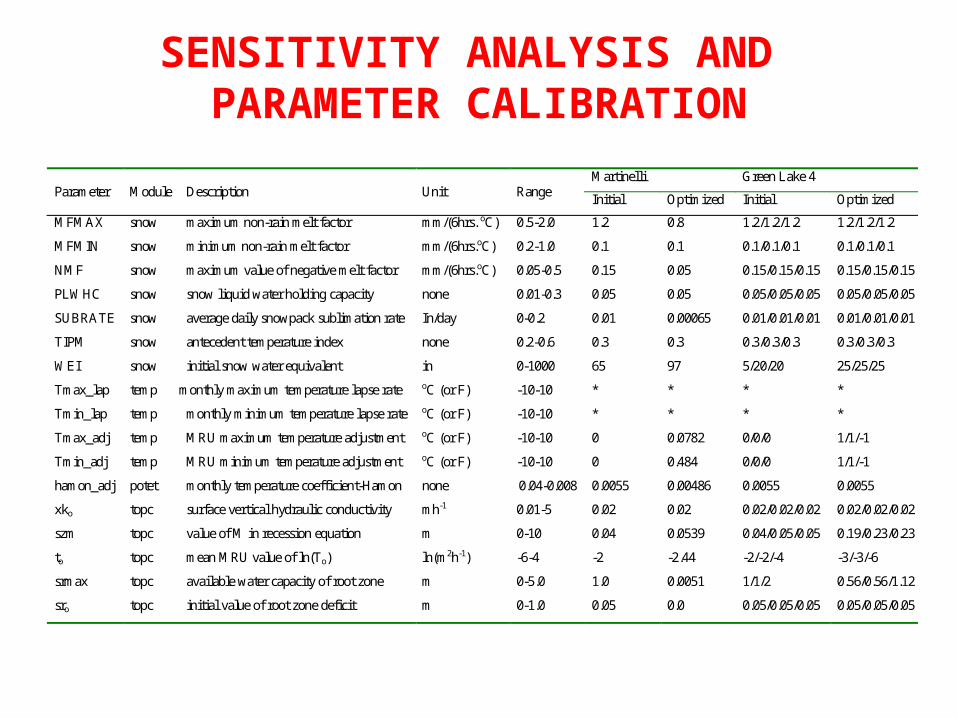
SENSITIVITY ANALYSIS AND PARAMETER CALIBRATION

Martinelli Green Lake 4Parameter Module Description Unit Range

Initial Optimized Initial Optimized

MFMAX snow maximum non-rain melt factor mm/(6hrs. oC) 0.5-2.0 1.2 0.8 1.2/1.2/1.2 1.2/1.2/1.2

MFMIN snow minimum non-rain melt factor mm/(6hrs.oC) 0.2-1.0 0.1 0.1 0.1/0.1/0.1 0.1/0.1/0.1

NMF snow maximum value of negative melt factor mm/(6hrs.oC) 0.05-0.5 0.15 0.05 0.15/0.15/0.15 0.15/0.15/0.15

PLWHC snow snow liquid water holding capacity none 0.01-0.3 0.05 0.05 0.05/0.05/0.05 0.05/0.05/0.05

SUBRATE snow average daily snowpack sublimation rate In/day 0-0.2 0.01 0.00065 0.01/0.01/0.01 0.01/0.01/0.01

TIPM snow antecedent temperature index none 0.2-0.6 0.3 0.3 0.3/0.3/0.3 0.3/0.3/0.3

WEI snow initial snow water equivalent in 0-1000 65 97 5/20/20 25/25/25

Tmax_lap temp monthly maximum temperature lapse rate oC (or F) -10-10 * * * *

Tmin_lap temp monthly minimum temperature lapse rate oC (or F) -10-10 * * * *

Tmax_adj temp MRU maximum temperature adjustment oC (or F) -10-10 0 0.0782 0/0/0 1/1/-1

Tmin_adj temp MRU minimum temperature adjustment oC (or F) -10-10 0 0.484 0/0/0 1/1/-1

hamon_adj potet monthly temperature coefficient-Hamon none 0.04-0.008 0.0055 0.00486 0.0055 0.0055

xko topc surface vertical hydraulic conductivity mh-1 0.01-5 0.02 0.02 0.02/0.02/0.02 0.02/0.02/0.02

szm topc value of M in recession equation m 0-10 0.04 0.0539 0.04/0.05/0.05 0.19/0.23/0.23

to topc mean MRU value of ln(To) ln(m2h-1) -6-4 -2 -2.44 -2/-2/-4 -3/-3/-6

srmax topc available water capacity of root zone m 0-5.0 1.0 0.0051 1/1/2 0.56/0.56/1.12

sro topc initial value of root zone deficit m 0-1.0 0.05 0.0 0.05/0.05/0.05 0.05/0.05/0.05

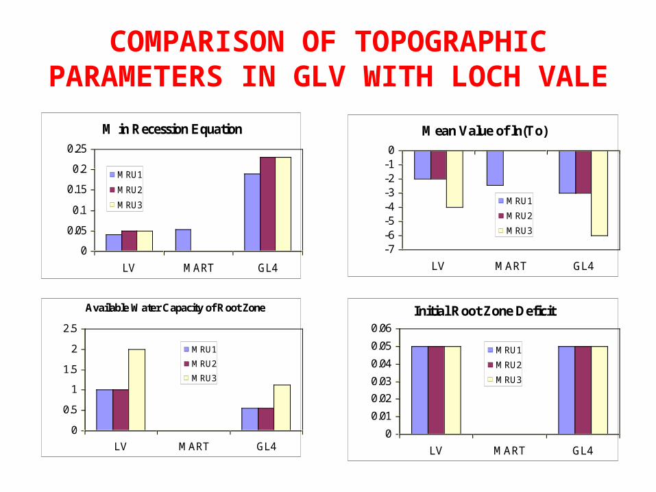
COMPARISON OF TOPOGRAPHIC PARAMETERS IN GLV WITH LOCH VALE

M in Recession Equation

0

0.05

0.1

0.15

0.2

0.25

LV MART GL4

SZM (m)

MRU1

MRU2

MRU3

Mean Value of ln(To)

-7-6-5-4-3-2-10

LV MART GL4

to (ln(m

2 h-1))

MRU1

MRU2

MRU3

Available Water Capacity of Root Zone

0

0.5

1

1.5

2

2.5

LV MART GL4

srmax (m)

MRU1

MRU2

MRU3

Initial Root Zone Deficit

0

0.01

0.02

0.03

0.04

0.05

0.06

LV MART GL4

sro

MRU1

MRU2

MRU3

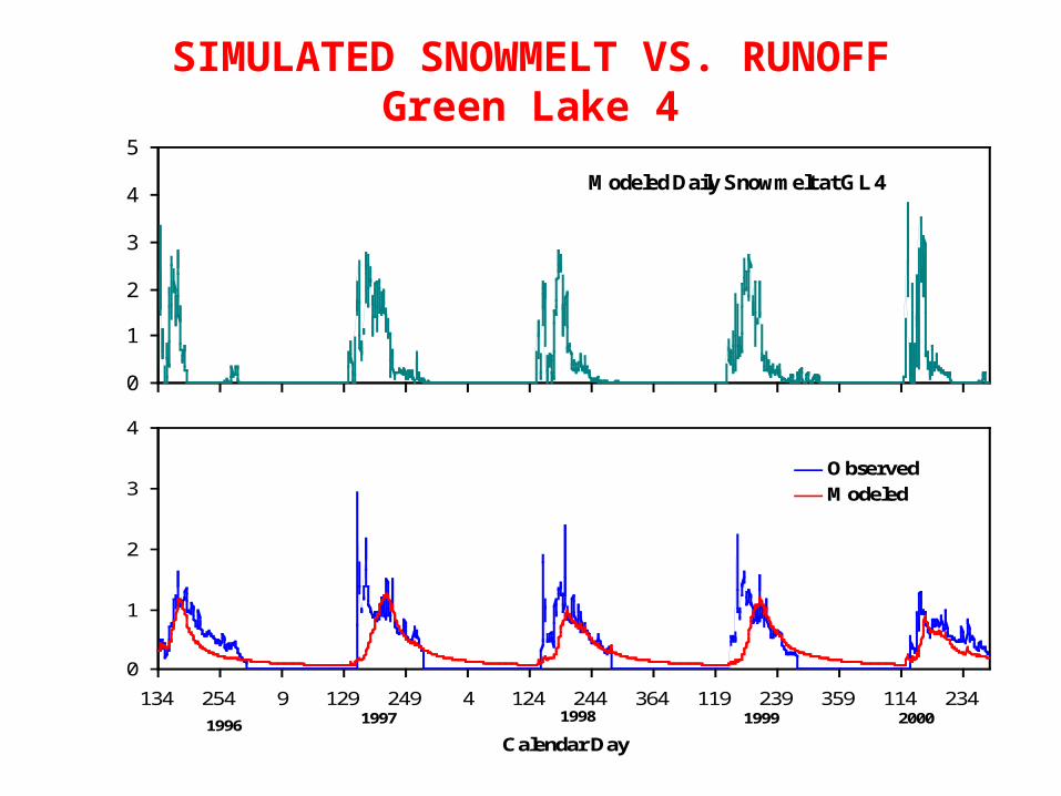
SIMULATED SNOWMELT VS. RUNOFFGreen Lake 4

0

1

2

3

4

134 254 9 129 249 4 124 244 364 119 239 359 114 234

Calendar Day

Runoff (cm)

Observed

Modeled

1997 1998 1999 20001996

Modeled Daily Snowmelt at GL4

0

1

2

3

4

5

SNowmelt (cm)

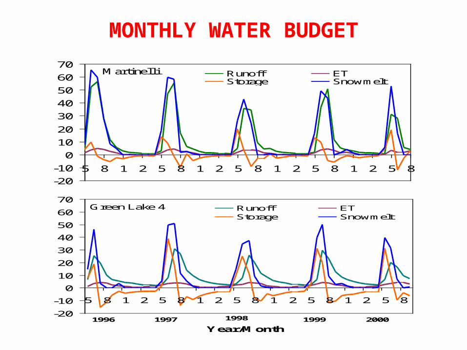
MONTHLY WATER BUDGET

-20

-10

0

10

20

30

40

50

60

70

5 8 1 2 5 8 1 2 5 8 1 2 5 8 1 2 5 8Water Balance Components (cm)

Runoff ETStorage Snowmelt

Martinelli

-20

-10

0

10

20

30

40

50

60

70

5 8 1 2 5 8 1 2 5 8 1 2 5 8 1 2 5 8

Year/Month

Water Balance Components (cm)

Runoff ETStorage Snowmelt

1996 1997 1998 1999 2000

Green Lake 4

PROBLEM ON RUNOFF SIMULATION

• Runoff peaks in May and June failed to be captured by the model

• The modeled runoff tells us that a large amount of snowmelt was infiltrated into soil to increase soil water storage

• However, the reality is that there were runoff peaks in May and June as observed

• It is hypothesized that a large amount of the snowmelt produced in May and June may contribute to the stream flow via overland and topsoil flowpaths due to impermeable barrier of frozen soils and basal ice

Summary and Conclusions

• Modeling system centered on TOPMODEL for representation of spatially distributed water balance based upon topography and GIS data (vegetation and soils).

• Capability to automatically set up and run at different model element scales.

• Encouraged by small scale calibration, though physical interpretation of calibrated parameters is problematic.

• Large scale water balance problem due to difficulty relating precipitation to topography had to be resolved using rather empirical adjustment method.

• Results provide hourly simulations of streamflow over the entire watershed.

MODFLOW

• THE IDEAL SITUATION FOR GROUNDWATER TYPES WOULD BE TO COMBINE PRMS WITH MODFLOW

• MODFLOW-PRMS CONNECTION IS BEING DONE TODAY

• BETA VERSIONS NOT YET AVAILABLE, BUT SOON

Are there any questions ?

AREA 1AREA 1

AREA 2AREA 2

3

12

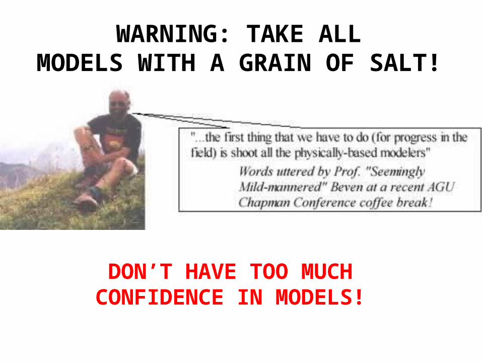
DON’T HAVE TOO MUCHCONFIDENCE IN MODELS!

WARNING: TAKE ALLMODELS WITH A GRAIN OF SALT!

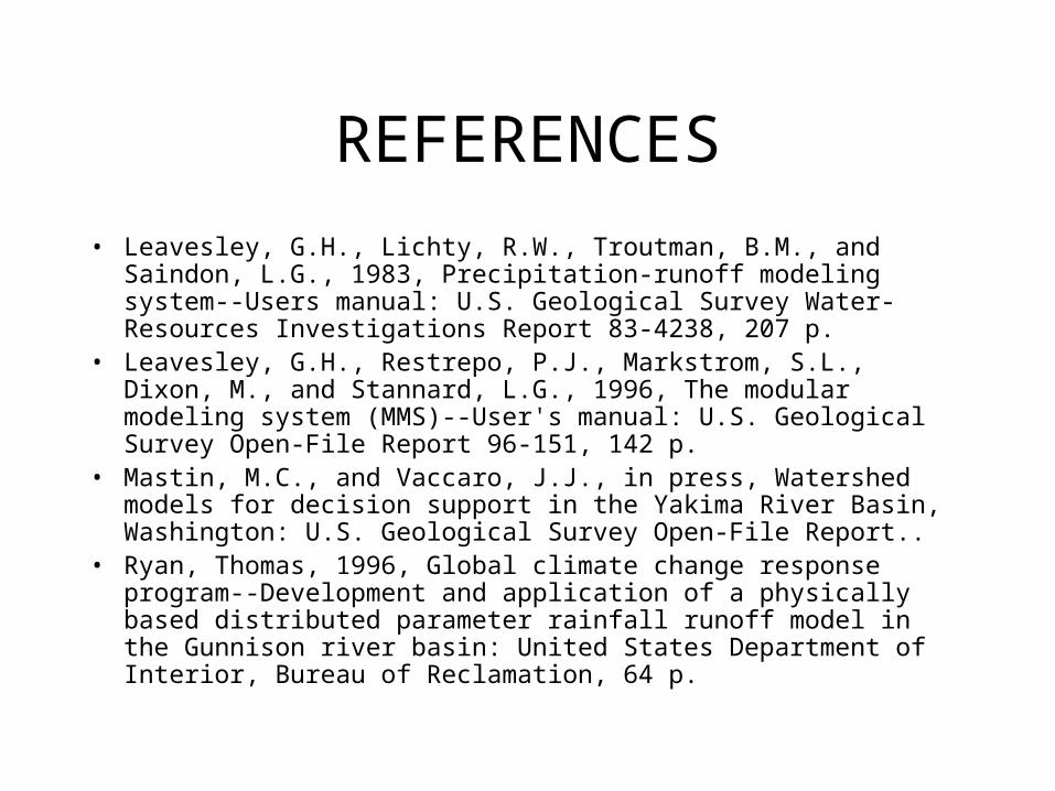
REFERENCES

• Leavesley, G.H., Lichty, R.W., Troutman, B.M., and Saindon, L.G., 1983, Precipitation-runoff modeling system--Users manual: U.S. Geological Survey Water-Resources Investigations Report 83-4238, 207 p.

• Leavesley, G.H., Restrepo, P.J., Markstrom, S.L., Dixon, M., and Stannard, L.G., 1996, The modular modeling system (MMS)--User's manual: U.S. Geological Survey Open-File Report 96-151, 142 p.

• Mastin, M.C., and Vaccaro, J.J., in press, Watershed models for decision support in the Yakima River Basin, Washington: U.S. Geological Survey Open-File Report..

• Ryan, Thomas, 1996, Global climate change response program--Development and application of a physically based distributed parameter rainfall runoff model in the Gunnison river basin: United States Department of Interior, Bureau of Reclamation, 64 p.

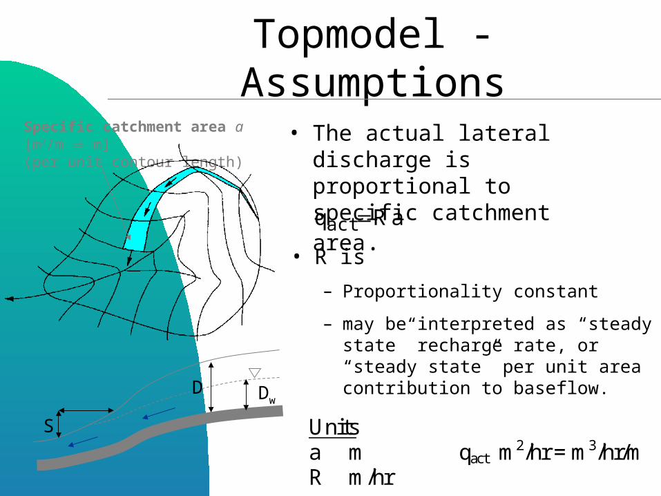
Topmodel - Assumptions

• The actual lateral discharge is proportional to specific catchment area.

aRqact =

Unitsa mR m/hr

qact m2/hr = m3/hr/m

Specific catchment area a [m2/m m] (per unit contour length)

S

DwD

• R is

– Proportionality constant

– may be interpreted as “steady state” recharge rate, or “steady state” per unit area contribution to baseflow.

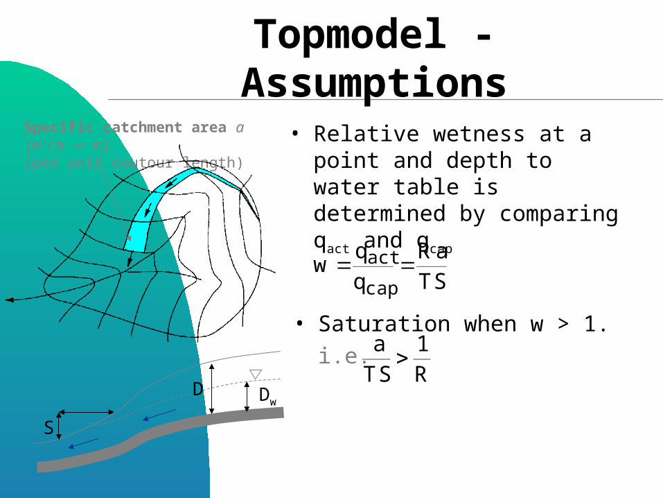
Topmodel - Assumptions

• Relative wetness at a point and depth to water table is determined by comparing qact and qcap

STaR

q

qw

cap

act ==

Specific catchment area a [m2/m m] (per unit coutour length)

S

DwD

• Saturation when w > 1.

i.e. R1

STa >

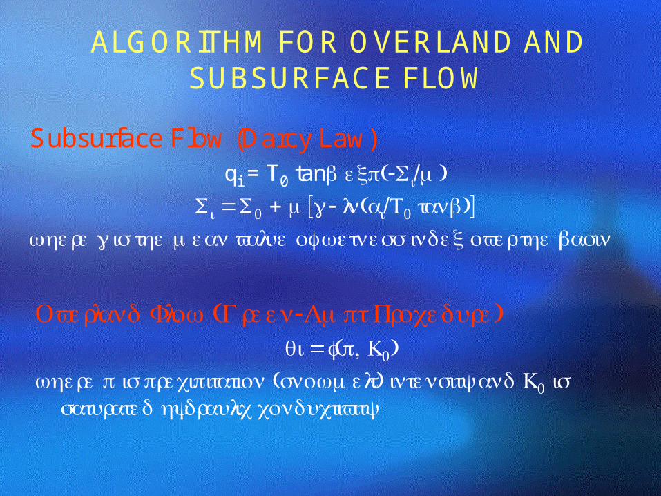
ALGORITHM FOR OVERLAND AND SUBSURFACE FLOW

Subsurface Flow (Darcy Law)qi = T0 tan exp(-Si/m)

Si =S0 +m[γ- ln(ai/T0 tan)]whereγ isthemeanvalueofwetnessindexoverthebasin

OverlandFlow(Green-AmptProcedure)qi=f(p,K0)

wherepisprecipitation(snowmelt)intensityandK0 issaturatedhydraulicconductivity