process capability > masterclass webinar

www.smallpeice.com

T. +44 (0)1926 336423

E: [email protected] a division of GP Strategies Limited

Process Capability

> Masterclass Webinar

© Smallpeice Enterprises © Smallpeice Enterprises © Smallpeice Enterprises © Smallpeice Enterprises

www.smallpeice.com www.smallpeice.com www.smallpeice.com www.smallpeice.com



Microphone Mute vs Unmute: Microphone Mute vs Unmute: Microphone Mute vs Unmute: Microphone Mute vs Unmute: please default to mute for your audio at all

times, and then ‘Unmute’ when asking or answering a question.

Virtual Session FormatVirtual Session FormatVirtual Session FormatVirtual Session Format

0830 0830 0830 0830 –––– 1600160016001600 Training Training Training Training Session Session Session Session

Lunch: 12:30 – 1:30pm



Content Agenda for Content Agenda for Content Agenda for Content Agenda for Masterclass Masterclass Masterclass Masterclass

Assessing Process ControlAssessing Process ControlAssessing Process ControlAssessing Process Control

Control Charts in MinitabControl Charts in MinitabControl Charts in MinitabControl Charts in Minitab

Process Capability for Attribute DataProcess Capability for Attribute DataProcess Capability for Attribute DataProcess Capability for Attribute Data

Rolled Throughput YieldRolled Throughput YieldRolled Throughput YieldRolled Throughput Yield

Process Capability for Variable DataProcess Capability for Variable DataProcess Capability for Variable DataProcess Capability for Variable Data

Basic Statistics FundamentalsBasic Statistics FundamentalsBasic Statistics FundamentalsBasic Statistics Fundamentals

www.smallpeice.com

T. +44 (0)1926 336423


Section 1

Introduction and Basic Statistics

This lesson introduces some important statistical

concepts that are essential for the understanding of

how control charts and process capability are

constructed and interpreted.





By the end of this section you should be able to:By the end of this section you should be able to:By the end of this section you should be able to:By the end of this section you should be able to:

Section ObjectivesSection ObjectivesSection ObjectivesSection Objectives

Understand the need for Basic Statistics

Understand different types of variation

Know the anatomy & main types of control charts

Apply control charts correctly

Calculate capability for continuous data

Calculate capability for attribute data

IsIsIsIs

measurement measurement measurement measurement

system(system(system(system(ssss) improvement) improvement) improvement) improvement

required?required?required?required?

Measure Phase RoadmapMeasure Phase RoadmapMeasure Phase RoadmapMeasure Phase Roadmap

MMMM

EEEE

AAAA

SSSS

UUUU

RRRR

EEEE

•Detailed process maps

•Process FMEA

UnderstandUnderstandUnderstandUnderstand

‘As‘As‘As‘As----Is’ processIs’ processIs’ processIs’ process

•Data collection plan

•Cause and Effect Diagram

(Fishbone)

Plan data Plan data Plan data Plan data

collectioncollectioncollectioncollection

•Measurement

system analysis

Confirm/validate Confirm/validate Confirm/validate Confirm/validate


systemssystemssystemssystems

•Root cause analysis tools•Operational Definitions•Mistake Proofing

•Standard Operating Procedures

Improve measurement Improve measurement Improve measurement Improve measurement


YESYESYESYES

NONONONO

YESYESYESYESIs Is Is Is

process stable & process stable & process stable & process stable &

in control?in control?in control?in control?

•Control charts (on outputs)•FMEA

• Interim Control Plan

•Determine Sampling Plan

Establish stability Establish stability Establish stability Establish stability

and controland controland controland control

NONONONO

•Normality tests

•Capability analysis

Collect data and Collect data and Collect data and Collect data and

establish baseline establish baseline establish baseline establish baseline

performanceperformanceperformanceperformance

•Project charter

Finalise Finalise Finalise Finalise

improvement improvement improvement improvement

objectivesobjectivesobjectivesobjectives

Gate

Review

ANALYSE PHASEANALYSE PHASEANALYSE PHASEANALYSE PHASE





• When analysing data we begin by understanding the key statistics that

describe the data. These are central tendency, variability &

probability distribution

• The concept of central tendency is familiar to most people. It is often

computed as the “average” of a data set

• Explicitly measuring variability & understanding probability distribution is

unfamiliar to most people, but it is an important part of understanding

the nature of a measurement system

Descriptive StatisticsDescriptive StatisticsDescriptive StatisticsDescriptive Statistics



Mean

Mode

Median

The value(s) occurring most frequently in the set of data

The arithmetic average of the data set

The middle value when the data is arranged in ascending order

Basic Statistics “What is the Average?”Basic Statistics “What is the Average?”Basic Statistics “What is the Average?”Basic Statistics “What is the Average?”





Knowledge Check: Measures of LocationKnowledge Check: Measures of LocationKnowledge Check: Measures of LocationKnowledge Check: Measures of Location

For example for numbers 32, 33, 34, 34, 35, 37, 37, 39, 41, 44For example for numbers 32, 33, 34, 34, 35, 37, 37, 39, 41, 44For example for numbers 32, 33, 34, 34, 35, 37, 37, 39, 41, 44For example for numbers 32, 33, 34, 34, 35, 37, 37, 39, 41, 44

interact viaCHAT

What is the MEAN?

What is the MEDIAN?





Knowledge Check: Measures of LocationKnowledge Check: Measures of LocationKnowledge Check: Measures of LocationKnowledge Check: Measures of Location


MEAN = 366/10 = 36.6

MEDIAN = 32, 33, 34, 34, 35, 37, 37, 39, 41, 44

DNP

Median = 36



What Is Variation?What Is Variation?What Is Variation?What Is Variation?

Don’t worry, that rope is one Don’t worry, that rope is one Don’t worry, that rope is one Don’t worry, that rope is one

inch thick on the averageinch thick on the averageinch thick on the averageinch thick on the average

That’s not what I’m worried about!





Variability recognises that processes do not produce identical results

every time:

• Variability may be caused by

identifiable forces acting on the

process or by minute fluctuations

in the process itself

• Range, standard deviation, & variance

are common measures of variability

• Standard deviation is the square

root of variance. Standard

deviation is useful because it can

be in the same units of measure

as the mean

VariabilityVariabilityVariabilityVariability

VariabilityCount

Measure



Basic Statistics “What is the Basic Statistics “What is the Basic Statistics “What is the Basic Statistics “What is the Spread?”Spread?”Spread?”Spread?”

The average distance that each data is away from the mean

The difference between the smallest & largest value in the sample

The range of the middle 50% of the data points

Range

Standard Deviation

4, 4, 5, 5, 6, 6, 6, 7, 7, 8, 8, 8, 8, 9, 9, 11

Q1 = 5.5 Q3 = 8IQR = 2.5

Inter Quartile Range





Knowledge Check: Measures of SpreadKnowledge Check: Measures of SpreadKnowledge Check: Measures of SpreadKnowledge Check: Measures of Spread


interact viaCHAT

What is the RANGE?

What is the INTER-QUARTILE RANGE?





Knowledge Check: Measures of SpreadKnowledge Check: Measures of SpreadKnowledge Check: Measures of SpreadKnowledge Check: Measures of Spread


32, 33, 34, 34, 35, 37, 37, 39, 41, 44

DNP

Median

Q1 = 34 Q3 = 39

RANGE (spread) = 44 – 32 = 12

IQR = 39 – 34 = 5





Visualising the Statistics: Box PlotVisualising the Statistics: Box PlotVisualising the Statistics: Box PlotVisualising the Statistics: Box Plot

MedianIn

ter-Q

ua

rtile R

an

ge

Ra

ng

e

32

33

34

35

36

37

38

39

40

41

42

43

44



• An often used measure of variability is the Standard DeviationStandard DeviationStandard DeviationStandard Deviation

• The Standard Deviation is defined as follows:

• In a more intuitive definition, think of it as the “average distance from

each data point to the mean”

Standard DeviationStandard DeviationStandard DeviationStandard Deviation

PopulationStandard Deviation

SampleStandard Deviation

2

1

)(

=

µ−=σ

N

i

i

N

X

2

1 1

)(= −

−=

n

i

i

nxx

s





• Like the mean, the Standard Deviation takes all of the observed values

into account & is a measure of the deviation of each data point from

the mean

• Deviation = The distance between a data point & the mean

MeanMeanMeanMean

• The greater the dispersion, the bigger the deviations & the bigger the standard

('average') deviation

Standard DeviationStandard DeviationStandard DeviationStandard Deviation



Calculating Standard DeviationCalculating Standard DeviationCalculating Standard DeviationCalculating Standard Deviation

10

20

40

50

30

x

Data Setn = 5mean = 30



Calculating Standard DeviationCalculating Standard DeviationCalculating Standard DeviationCalculating Standard Deviation

x

10

20

40

50

30

( )xx - 2( )xx -

-20

-10

0

10

20

400

100

0

100

400

SSQ ∑ 10002( )xx -

Data Setn = 5mean = 30

(n-1) 4

Variance 250

Std Dev 15.81



• Many sets of data follow the normal

distribution or bell shaped curve.

One of the key properties of the

normal distribution is the

relationship between the shape of

the curve & the standard deviation

• 99.73% of the area of the Normal

distribution is contained between -

3 standard deviations & + 3

standard deviations from the mean

The Normal DistributionThe Normal DistributionThe Normal DistributionThe Normal Distribution



-1s

+1s+2s +3s

+4s-2s

-3s

-4s

x +5s +6s-6s

-5s

68.24%

99.999943%

99.9999998%

99.9973%

99.73%

95.45%

INFLECTION POINT

Properties of the Normal DistributionProperties of the Normal DistributionProperties of the Normal DistributionProperties of the Normal Distribution

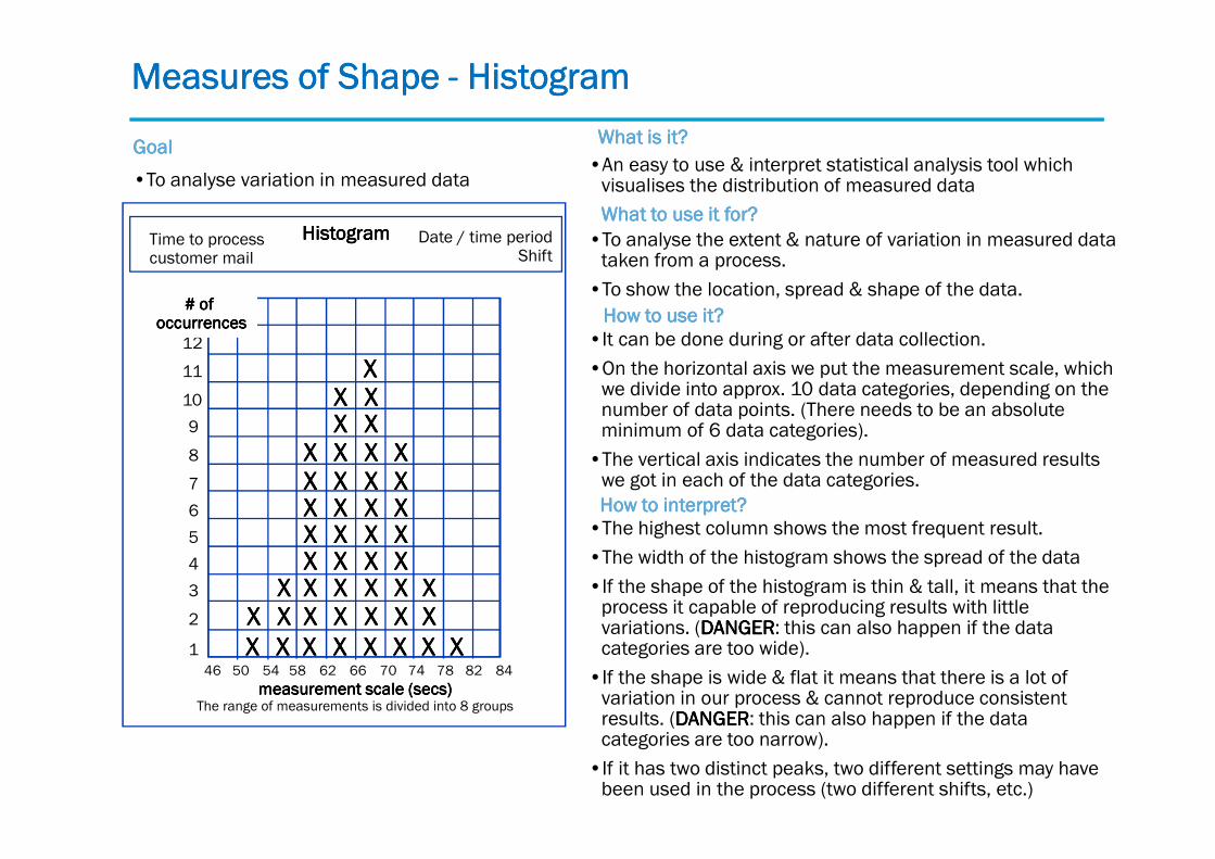
•To analyse variation in measured data

What is it?What is it?What is it?What is it?

•An easy to use & interpret statistical analysis tool which visualises the distribution of measured data

What to use it for?What to use it for?What to use it for?What to use it for?

•To analyse the extent & nature of variation in measured data taken from a process.

•To show the location, spread & shape of the data.

How to use it?How to use it?How to use it?How to use it?

•It can be done during or after data collection.

•On the horizontal axis we put the measurement scale, which we divide into approx. 10 data categories, depending on the number of data points. (There needs to be an absolute minimum of 6 data categories).

•The vertical axis indicates the number of measured results we got in each of the data categories.

XXXXXXXX

XXXXXXXX

XXXX

XXXXXXXX

XXXXXXXX

XXXX

XXXX

XXXXXXXX

XXXXXXXX

XXXX

XXXXXXXX

XXXXXXXX

XXXX

XXXXXXXXXXXX

XXXXXXXX

XXXX

XXXXXXXX

XXXXXXXX

XXXX

XXXXXXXX

XXXX

XXXXXXXX

XXXXXXXX

XXXX

XXXXXXXXXXXX

XXXXXXXXXXXX

11

1

2

10

9

6

4

3

8

7

5

12

6254 58 70 74 7850 66 82 8446

measurement scale (secs)measurement scale (secs)measurement scale (secs)measurement scale (secs)The range of measurements is divided into 8 groups

# of# of# of# ofoccurrencesoccurrencesoccurrencesoccurrences

How to interpret?How to interpret?How to interpret?How to interpret?•The highest column shows the most frequent result.

•The width of the histogram shows the spread of the data

•If the shape of the histogram is thin & tall, it means that the process it capable of reproducing results with little variations. (DANGERDANGERDANGERDANGER: this can also happen if the data categories are too wide).

•If the shape is wide & flat it means that there is a lot of variation in our process & cannot reproduce consistent results. (DANGERDANGERDANGERDANGER: this can also happen if the data categories are too narrow).

•If it has two distinct peaks, two different settings may have been used in the process (two different shifts, etc.)

HistogramHistogramHistogramHistogram Date / time periodShift

Time to processcustomer mail

GoalGoalGoalGoal

Measures of Shape Measures of Shape Measures of Shape Measures of Shape ---- HistogramHistogramHistogramHistogram

11

10

9

8

7

6

5

4

3

2

1

0

Count

5 87 9 10 11 13126 14

seconds

5

5

5

5 8 9 10 1211 13 1476

6

6

6

6

6

7

7

7

7

7

7

7

7

7

7

8

8

8

8

8

8

9

9

9

9

10

10

10 12

11

11

Creating a HistogramCreating a HistogramCreating a HistogramCreating a Histogram





Important information we

get from evaluating the

shape of the distribution

• Visual display of the

location & variability

• How much of the

distribution falls outside

the customer requirements

• Evidence of specific factors that are contributing to variation in the

process output

• Evidence about whether the distribution follows a classic bell-shape,

thereby allowing standard statistical testing & prediction of defect levels &

capability

How is my Data Distributed?How is my Data Distributed?How is my Data Distributed?How is my Data Distributed?

10 11 12 13 14 15 16 17 18 19

0

5

10

Frequency

Frequency

Frequency

Frequency

Call Center A

N = 100

Average = 14.617

Std Dev = 2.212

10 15 20

0

10

20

Frequency

Call Center B

N = 100

Average = 14.536

Std Dev = 2.266

Example:Example:Example:Example:

You are evaluating two call centres

last 100 calls for queue time. There

is no significant difference between

the average & standard deviation

in queue times. Is one of the centres

performing better than the other?

Measures of location & variability are not always going Measures of location & variability are not always going Measures of location & variability are not always going Measures of location & variability are not always going

to tell you the whole storyto tell you the whole storyto tell you the whole storyto tell you the whole story

How is my Data Distributed?How is my Data Distributed?How is my Data Distributed?How is my Data Distributed?

Just looking at the histogram shape Just looking at the histogram shape Just looking at the histogram shape Just looking at the histogram shape

gives you useful information about the gives you useful information about the gives you useful information about the gives you useful information about the

processprocessprocessprocess



Measures of ShapeMeasures of ShapeMeasures of ShapeMeasures of Shape

When describing the shape of a distribution there is some specific

terminology we can use:

SkewSkewSkewSkew

BiBiBiBi----modalmodalmodalmodal



What might these distribution shapes tell us?What might these distribution shapes tell us?What might these distribution shapes tell us?What might these distribution shapes tell us?

ServiceServiceServiceService Level Level Level Level

AgreementAgreementAgreementAgreement

Understanding ShapeUnderstanding ShapeUnderstanding ShapeUnderstanding Shape

A B

Cinteract viaCHAT

EXERCISE

29

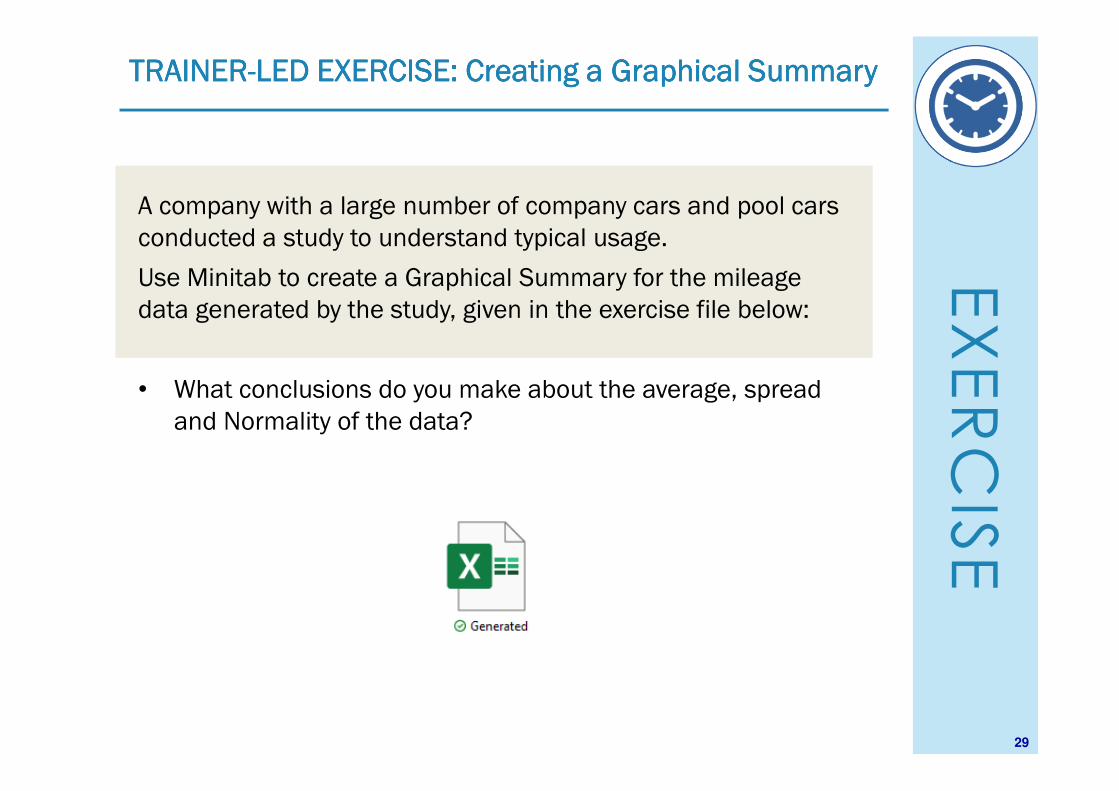
TRAINERTRAINERTRAINERTRAINER----LED LED LED LED EXERCISE: Creating a Graphical Summary EXERCISE: Creating a Graphical Summary EXERCISE: Creating a Graphical Summary EXERCISE: Creating a Graphical Summary

A company with a large number of company cars and pool cars

conducted a study to understand typical usage.

Use Minitab to create a Graphical Summary for the mileage

data generated by the study, given in the exercise file below:

• What conclusions do you make about the average, spread

and Normality of the data?



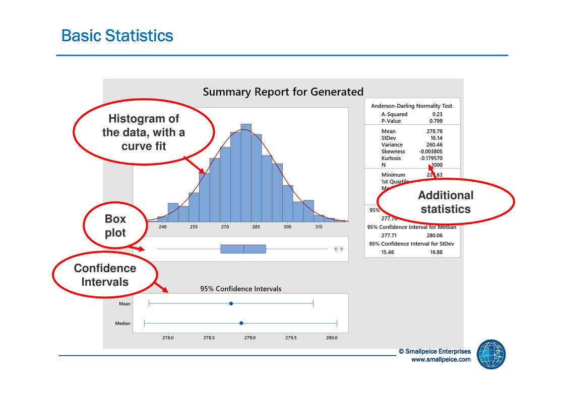
Basic Statistics: Graphical Summary Basic Statistics: Graphical Summary Basic Statistics: Graphical Summary Basic Statistics: Graphical Summary

Select Graphical Summary

from Basic Statistics



Basic StatisticsBasic StatisticsBasic StatisticsBasic Statistics

Additional statistics

Histogram of the data, with a

curve fit

Box plot

Confidence Intervals



1 st Quartile 20.000

Median 25.000

3rd Quartile 27.000

Maximum 35.000

22.669 25.931

23.000 27.000

4.795 7.1 53

A-Squared 0.92

P-Value 0.018

Mean 24.300

StDev 5.740

Variance 32.949

Skewness -0.345902

Kurtosis -0.277666

N 50

Minimum 1 3.000

Anderson-Darling Normality Test

95% Confidence Interval for Mean

95% Confidence Interval for Median

95% Confidence Interval for StDev

3530252015

Median

Mean

2726252423

95% Confidence Intervals

Summary Report for Time to Complete Application

Anderson Darling TestAnderson Darling TestAnderson Darling TestAnderson Darling Test

Use the descriptive statistics to test for Normality, examine the shape of

the data, look for outliers & then look at the P value, if the P value is <

0.05 then the data is not Normal. Is the P value is >0.05 then we can fit

the Normal distribution to the data.

P value is

displayed here

EXERCISE

33

OPTIONAL OPTIONAL OPTIONAL OPTIONAL EXERCISEEXERCISEEXERCISEEXERCISE: Creating a Graphical Summary : Creating a Graphical Summary : Creating a Graphical Summary : Creating a Graphical Summary

A commuter has collected data on their fuel consumption for

each car journey to and from work.

The metric is Miles per Gallon (mpg)

Use Minitab to create a Graphical Summary for the MPG data

generated by the study, given in the exercise file below:

• What conclusions do you make about the location, spread

and shape of the data?

Group EXERCISE

10 minutes

Refer to Data File – Fuel Consumption

www.smallpeice.com

T. +44 (0)1926 336423


Section 2

Assessing Process Control

This lesson introduces some important concepts that

will help you understand how process stability can be

achieved.



• A key check in the measure phase is whether the process is stable

• A stable process is predictable over time and so can be base-lined and improved

• An unstable process is technically ‘out of control’ and therefore must be stabilized as a first step




Data AnalysisData AnalysisData AnalysisData Analysis

• If the process is a regular, repetitive process with a measurable output

(such as time taken to conduct a repetitive process step) then Statistical

Process Control Charts (SPC) can be used to assess process stability

Process AnalysisProcess AnalysisProcess AnalysisProcess Analysis

• If the process is non-repetitive or low volume then process audit

techniques can be used to establish if there is a clearly documented

process which is consistently complied with

Two Approaches to Assessing StabilityTwo Approaches to Assessing StabilityTwo Approaches to Assessing StabilityTwo Approaches to Assessing Stability



Common Cause

Special Cause

Type of VariationType of VariationType of VariationType of Variation DefinitionDefinitionDefinitionDefinition CharacteristicsCharacteristicsCharacteristicsCharacteristics

Process is stable and

predictable

Process displays

variation outside

what is expected

(process is not

stable/out of control)

• Expected

• Predictable range of values

• Random causes of variation

• Unexpected

• Unpredictable range of values

• Non-Random (assignable) causes of variation

Reminder Common vs Special CauseReminder Common vs Special CauseReminder Common vs Special CauseReminder Common vs Special Cause



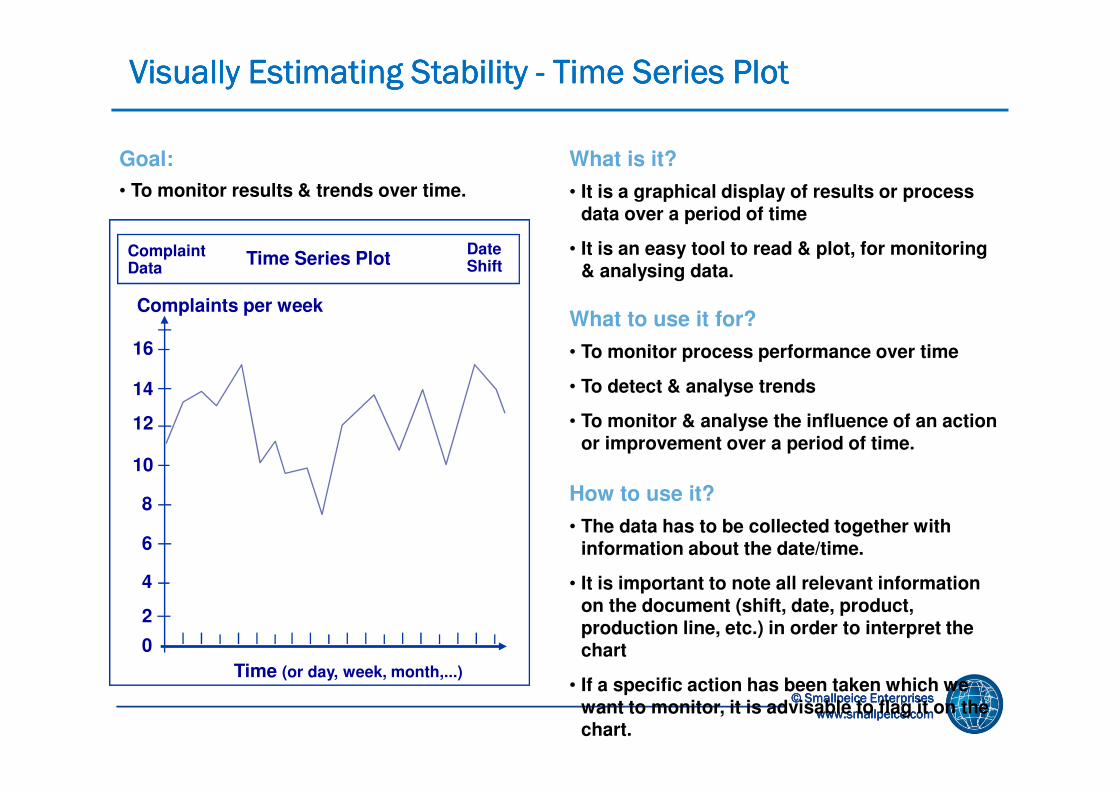
Goal:

• To monitor results & trends over time.

What is it?

• It is a graphical display of results or process data over a period of time

• It is an easy tool to read & plot, for monitoring & analysing data.

What to use it for?

• To monitor process performance over time

• To detect & analyse trends

• To monitor & analyse the influence of an action or improvement over a period of time.

How to use it?

• The data has to be collected together with information about the date/time.

• It is important to note all relevant information on the document (shift, date, product, production line, etc.) in order to interpret the chart

• If a specific action has been taken which we want to monitor, it is advisable to flag it on the chart.

Time (or day, week, month,...)

Complaints per week

0

16

10

Time Series PlotDateShift

Complaint Data

4

6

8

12

14

2

Visually Estimating Stability Visually Estimating Stability Visually Estimating Stability Visually Estimating Stability ---- Time Series PlotTime Series PlotTime Series PlotTime Series Plot



Checks for StabilityChecks for StabilityChecks for StabilityChecks for Stability

• If data is collected over a period of time, process stability can be checked by looking at some form of time series plot

• We look for four indicators that the process is not stable:

SpikesSpikesSpikesSpikesTrendsTrendsTrendsTrends

ShiftsShiftsShiftsShifts PatternsPatternsPatternsPatterns



Be Careful Be Careful Be Careful Be Careful –––– Scales can be MisleadingScales can be MisleadingScales can be MisleadingScales can be Misleading

Which of these two processes looks the most stable?Which of these two processes looks the most stable?Which of these two processes looks the most stable?Which of these two processes looks the most stable?

Actually this is the exact same data set plotted on two Actually this is the exact same data set plotted on two Actually this is the exact same data set plotted on two Actually this is the exact same data set plotted on two

different scales!different scales!different scales!different scales!

4036322824201 61 284

50.0

47.5

45.0

42.5

40.0

37.5

35.0

Index

Tim

e

Time Series Plot of Time

4036322824201 61 284

70

60

50

40

30

20

1 0

0

Index

Tim

e

Time Series Plot of Time



Checking Stability Checking Stability Checking Stability Checking Stability –––– Control ChartsControl ChartsControl ChartsControl Charts

To remove the error of judgement which can be caused by scales, etc. a special

type of time series plot, known as a control chart (or Statistical Process Control

Chart ) can be used to identify the presence of special cause variation

Successive SamplesSuccessive SamplesSuccessive SamplesSuccessive Samples

Process AverageProcess AverageProcess AverageProcess Average

Upper Control LimitUpper Control LimitUpper Control LimitUpper Control Limit

Lower Control LimitLower Control LimitLower Control LimitLower Control Limit

+3s+3s+3s+3s

----3s3s3s3s



1 point > 3 standard deviations from the 1 point > 3 standard deviations from the 1 point > 3 standard deviations from the 1 point > 3 standard deviations from the

centre linecentre linecentre linecentre line

9 points in a row on same side of the 9 points in a row on same side of the 9 points in a row on same side of the 9 points in a row on same side of the

centre linecentre linecentre linecentre line

6 points in a row, all increasing or all 6 points in a row, all increasing or all 6 points in a row, all increasing or all 6 points in a row, all increasing or all

decreasingdecreasingdecreasingdecreasing

14 points in a row, alternating14 points in a row, alternating14 points in a row, alternating14 points in a row, alternating

up & downup & downup & downup & down

Statistical Tests for Special Causes (All Control Charts)Statistical Tests for Special Causes (All Control Charts)Statistical Tests for Special Causes (All Control Charts)Statistical Tests for Special Causes (All Control Charts)

EXERCISE

Chart 1:Chart 1:Chart 1:Chart 1:

Chart 3:Chart 3:Chart 3:Chart 3: Chart 4:Chart 4:Chart 4:Chart 4:

Chart 2:Chart 2:Chart 2:Chart 2:

Interpret the following Control Charts:Interpret the following Control Charts:Interpret the following Control Charts:Interpret the following Control Charts:

EXERCISE: EXERCISE: EXERCISE: EXERCISE: Control Chart InterpretationControl Chart InterpretationControl Chart InterpretationControl Chart Interpretation

A B

C D



When using control charts, make a note on the chart when anything happens

which might affect the process:

• changes in personnel

• changes in procedure

• changes to products, services, terms & conditions, etc.

• changes to computer systems & software

• changes to materials, consumables, etc.

• network faults, system failures, etc.

Process LogsProcess LogsProcess LogsProcess Logs

Notes are essential to interpretation & improvement actionNotes are essential to interpretation & improvement actionNotes are essential to interpretation & improvement actionNotes are essential to interpretation & improvement action



This is what it’s all about!!This is what it’s all about!!This is what it’s all about!!This is what it’s all about!!

• Control charts are only a means to an end

• Control charts are a proactive tool for highlighting when something is

happening in your process to risk it becoming unstable...

• Without effective improvement action, control charts have no value

• Prompt action is essential!

• Seek a permanent solution wherever possible

• Recalculate limits after eliminating a problem

Action After InterpretationAction After InterpretationAction After InterpretationAction After Interpretation



Control Chart SelectorControl Chart SelectorControl Chart SelectorControl Chart Selector

Individuals or

Subgroups?

I-MR Chart X-bar & R Chart

IND S/G

VARIABLES

Start

Data Type?

Defects or Defectives?

Constant Sample Size?


p-Chartnp-Chartu-Chartc-Chart

YES YESNO NO

DEFECTS DEFECTIVES

ATTRIBUTES

We will consider all of these We will consider all of these We will consider all of these We will consider all of these

chartschartschartscharts

Let’s start here

www.smallpeice.com

T. +44 (0)1926 336423


Section 3

Control Charts in Minitab

This lesson guides you through the process of

producing charts in Minitab.



Example:Example:Example:Example: What is it?What is it?What is it?What is it?

• A pair of control charts for monitoring processes from which individual data points are taken


• The I (individual values) chart is used to monitor the setting & the MR (moving range) chart to monitor the variability of a process from which individual data points are taken


• Define & check the measurement system• Determine sampling frequency• Collect initial data (ideally 25 or more data points)• Plot the data points on the I chart in time order• Plot the difference between successive data points on

the MR chart• Calculate & plot the process average (Xbar) on the I

chart & the average moving range (MRbar) on the MR chart

• Calculate & plot the control limits for both charts• Apply tests to detect special causes of variation• Take action to eliminate special causes of variation,

then recalculate centrelines & control limits• Continue to collect & plot data, addressing special

causes of variation if & when they occur

IIII----MR ChartsMR ChartsMR ChartsMR Charts

Formulae:Formulae:Formulae:Formulae:

• E2, D3 & D4 are factors used in the calculation

of control limits

• If adjacent values are used to calculate the

moving range (i.e. subgroup size = 2), the

factors are: E2=2.66, D3=0 & D4=3.267

Observation

In

div

idu

al

Va

lue

10997857361493725131

800

700

600

500

_X=610.2

UC L=710.8

LC L=509.6

Observation

Mo

vin

g R

an

ge

10997857361493725131

300

200

100

0

__MR=37.8

UC L=123.6

LC L=0

11111

1

1

1111

1

1

1

I-MR Chart of Cash Dispensed from ATMs

MREXUCL 2X +=

MREXLCL 2X −=

MRDUCL 4R =

MRDLCL 3R =



IMR Charts (Individual Moving Range)IMR Charts (Individual Moving Range)IMR Charts (Individual Moving Range)IMR Charts (Individual Moving Range)

Stat > Control Charts > Variables Chart for Individuals > IStat > Control Charts > Variables Chart for Individuals > IStat > Control Charts > Variables Chart for Individuals > IStat > Control Charts > Variables Chart for Individuals > I----MR …MR …MR …MR …



Individual and Moving Range ChartsIndividual and Moving Range ChartsIndividual and Moving Range ChartsIndividual and Moving Range Charts

EXERCISE

51

TRAINERTRAINERTRAINERTRAINER----LED LED LED LED EXERCISE: Creating an IEXERCISE: Creating an IEXERCISE: Creating an IEXERCISE: Creating an I----MR Chart MR Chart MR Chart MR Chart

A study has been carried out at a call centre, following

complaints that the waiting time seems be inconsistent.

Use Minitab to construct an I-MR Control chart for the data

given in the file below:

• What conclusions do you make?

• Are any actions needed? If so, what?

EXERCISE

52

OPTIONAL OPTIONAL OPTIONAL OPTIONAL EXERCISEEXERCISEEXERCISEEXERCISE: Creating a : Creating a : Creating a : Creating a Individuals ChartIndividuals ChartIndividuals ChartIndividuals Chart

A commuter has collected data on their fuel consumption for

each car journey to and from work.

The metric is Miles per Gallon (mpg)

Use Minitab to create an Individual Chart for the MPG data

generated by the study, given in the exercise file below:

• Is the fuel consumption stable over time?

Group EXERCISE

10 minutes

Refer to Data File – Fuel Consumption




• A pair of control charts for monitoring processes from which subgroups of data are taken


• The Xbar (averages) chart is used to monitor the setting & the R (range) chart to monitor the variability of a process from which subgroups of data are taken


• Define & check the measurement system• Determine subgroup size & sampling frequency• Collect initial data (ideally 25 or more subgroups)• Calculate & plot the subgroup averages on the Xbar

chart in time order• Plot the subgroup ranges on the R chart• Calculate & plot the process average (X double bar) on

the Xbar chart & the average range (Rbar) on the R chart

• Calculate & plot the control limits for both charts• Apply tests to detect special causes of variation• Take action to eliminate special causes of variation,

then recalculate centrelines & control limits• Continue to collect & plot data, addressing special


XbarXbarXbarXbar----R ChartsR ChartsR ChartsR Charts


• A2, D3 & D4 are factors used in the calculation of control limits

• Factor values depend on subgroup size

RAXUCL 2X+=

RAXLCL 2X−=

RDUCL 4R =

RDLCL 3R =

Subgroup

Size A2 D3 D4

2 1.880 0 3.267

3 1.023 0 2.574

4 0.729 0 2.282

5 0.577 0 2.114

Sample

Sa

mp

le M

ea

n

252321191715131197531

4.02

4.00

3.98

__X=4.00058

UCL=4.02099

LCL=3.98017

Sample

Sa

mp

le R

an

ge

252321191715131197531

0.08

0.06

0.04

0.02

0.00

_R=0.03539

UCL=0.07482

LCL=0

6

1

6

1

Xbar-R Chart Print Density





• No hard & fast rules

• Samples of 5 commonly used: diminishing returns as sample size increases

• Samples must be produced under similar conditions & within a short time:

within-sample variation should reflect only the common causes of variation

• Ideally each from the same tool or head: separate multiple

heads/tools/stations for analysis purposes

Determine Subgroup SizeDetermine Subgroup SizeDetermine Subgroup SizeDetermine Subgroup Size

EXERCISE

55

TRAINERTRAINERTRAINERTRAINER----LED LED LED LED EXERCISE: Creating an EXERCISE: Creating an EXERCISE: Creating an EXERCISE: Creating an XbarXbarXbarXbar & R Chart & R Chart & R Chart & R Chart

A process used to produce slots in components required for

assembly is under investigation.

Use Minitab to construct an Xbar-R Control chart for the data

given in the exercise file below:

• What conclusions do you make?

• Are any actions needed? If so, what?



XbarXbarXbarXbar----R Charts in MinitabR Charts in MinitabR Charts in MinitabR Charts in Minitab

Stat > Control Charts > Variables Chart for Subgroups > Stat > Control Charts > Variables Chart for Subgroups > Stat > Control Charts > Variables Chart for Subgroups > Stat > Control Charts > Variables Chart for Subgroups > XbarXbarXbarXbar----R …R …R …R …



Selecting Tests for Variables Selecting Tests for Variables Selecting Tests for Variables Selecting Tests for Variables



Control Chart SelectorControl Chart SelectorControl Chart SelectorControl Chart Selector

Individuals or

Subgroups?

I-MR Chart X-bar & R Chart

IND S/G

VARIABLES

Start

Data Type?

Defects or Defectives?



p-Chartnp-Chartu-Chartc-Chart

YES YESNO NO

DEFECTS DEFECTIVES

ATTRIBUTES

We will consider all of these We will consider all of these We will consider all of these We will consider all of these

chartschartschartscharts

Let’s continue here



Common Attribute Control ChartsCommon Attribute Control ChartsCommon Attribute Control ChartsCommon Attribute Control Charts

Type of Chart

Variables or Attributes?

Description Example

np Number defective

A • The np chart is used for monitoring the

number of defective items in constant-sized samples taken from a process

• Number of parts in samples of 200 checked each day

P Proportion defective

A

• The p chart is used for monitoring the proportion of defective items in samples of varying sizes taken from a process

• Proportion of faulty cartridges in the process, in a full day’s production

C Number of

defects A

• The c chart is used for monitoring the number of defects in constant sized samples taken from a process

• Number of errors in samples of 50 assemblies checked each day

U Defects per

unit A

• The u chart is used for monitoring the number of defects found in samples of varying sizes taken from a process

• Number of errors in supplied materials each day, where the quantities vary from day to day



Control Chart Pop QuizControl Chart Pop QuizControl Chart Pop QuizControl Chart Pop Quiz

What type of control chart would you use for each What type of control chart would you use for each What type of control chart would you use for each What type of control chart would you use for each

of the following applications?of the following applications?of the following applications?of the following applications?

APPLICATIONAPPLICATIONAPPLICATIONAPPLICATION TYPE OF CHARTTYPE OF CHARTTYPE OF CHARTTYPE OF CHART

Number of missed deliveries per day (no. of deliveries varies)

No. of faults reported per day on the soldering machine

No. of defective mouldings in samples of 20 checked daily

No. of errors per production instruction (quantity processed each day varies)



Attribute Charts in MinitabAttribute Charts in MinitabAttribute Charts in MinitabAttribute Charts in Minitab

Stat > Control Charts > Attribute ChartsStat > Control Charts > Attribute ChartsStat > Control Charts > Attribute ChartsStat > Control Charts > Attribute Charts




• A control chart for monitoring the number of defective items in constant sized samples taken regularly from a process


• It is used when the number of defective items is the matter of interest, rather than the actual defects

• It is only applicable when the sample size cannot or does not vary


• Define & check the measurement system

• Determine the subgroup size & sampling frequency

• Collect initial data (ideally 25 or more subgroups)

• Plot the number of defective items in each subgroup on the chart in time order

• Calculate & plot the average number defective (np-bar) on the chart

• Calculate & plot the control limits

• Apply tests to detect special causes of variation

• Take action to eliminate special causes of variation, then recalculate centreline & control limits

• Continue to collect & plot data, addressing special causes of variation if & when they occur

Number Defective (np) ChartNumber Defective (np) ChartNumber Defective (np) ChartNumber Defective (np) Chart


where np1, np2 etc. are the number of defective items in each of the k subgroups

where n is the subgroup size

252219161310741

6

5

4

3

2

1

0

Sample

Sa

mp

le C

ou

nt

__NP=1.769

UCL=5.724

LCL=0

1

NP Chart of Incorrect Fitted Parts

k

np...npnpnp k21 +++

=

)n

np1(np3npUCLnp −+=

)n

np1(np3npLCLnp −−=



Number Defective (np) ChartNumber Defective (np) ChartNumber Defective (np) ChartNumber Defective (np) Chart

Note: right-clicking over the out-of-control point takes you to the Session Window, which indicates the test which has been failed

20/1

2/20

04

29/1

1/20

04

08/1

1/20

04

18/1

0/20

04

27/0

9/20

04

06/09/

2004

1 6/08/

2004

26/0

7/2004

05/0

7/2004

6

5

4

3

2

1

0

W/C

Sam

ple

Co

un

t

__

NP=1.769

UCL=5.724

LCL=0

1

NP Chart of Incorrect Fitted Parts



InstructorInstructorInstructorInstructor----led Exercise: np Chartsled Exercise: np Chartsled Exercise: np Chartsled Exercise: np Charts

• The worksheet lists the number of incorrect parts

found in a weekly audit of 100 parts produced

for stock

• Create & interpret an ‘np’ chart using:

In the ‘Options’ ‘Options’ ‘Options’ ‘Options’ box, select ‘Tests’ & ‘Perform all tests for special causes’

In the ‘ScaleScaleScaleScale’ box, select ‘Stamp’ & ‘W/C’




Proportion Defective (p) ChartProportion Defective (p) ChartProportion Defective (p) ChartProportion Defective (p) Chart



• A control chart for monitoring the proportion of defective items in samples of varying sizes taken regularly from a process


• It is used when the proportion of defective items is the matter of interest, rather than the actual defects

• It is applicable when the sample size cannot be held constant, e.g. when carrying out 100% checks


• Define & check the measurement system• Determine the sampling frequency• Collect initial data (ideally 25 or more subgroups)• Calculate & plot the proportion of defective items in

each subgroup on the chart in time order• Calculate & plot the average proportion defective (p-

bar) on the chart• Calculate & plot the control limits. (Note: this is best

done using Minitab, since control limit positions are dependent on subgroup size)

• Apply tests to detect special causes of variation• Take action to eliminate special causes of variation,

then recalculate centreline & control limits• Continue to collect & plot data, addressing special


where n1p1, n2p2 etc. are the number of defective items in each of the k subgroups, & n1, n2 etc. are the number of items checked in each subgroup

252321191715131197531

0.9

0.8

0.7

0.6

0.5

0.4

0.3

0.2

0.1

0.0

Sample

Pro

po

rtio

n

_P=0.160

UCL=0.454

LCL=0

1

1

P Chart of Incorrect Orders

Tests performed with unequal sample sizes

k21

kk2211

n...nn

pn...pnpnp

+++

+++=

n

)p1(p3pUCLp

−+=

n

)p1(p3pLCLp

−−=

EXERCISE

Group Exercise: Creating a PGroup Exercise: Creating a PGroup Exercise: Creating a PGroup Exercise: Creating a P----ChartChartChartChart

THE TASKTHE TASKTHE TASKTHE TASK

referring to the information provided in the Handout 01: referring to the information provided in the Handout 01: referring to the information provided in the Handout 01: referring to the information provided in the Handout 01:

Use Minitab to create a pUse Minitab to create a pUse Minitab to create a pUse Minitab to create a p----chart and interpret the resultschart and interpret the resultschart and interpret the resultschart and interpret the results

‘HOW TO’ ‘HOW TO’ ‘HOW TO’ ‘HOW TO’ Instructions for working in your group:

• Elect a facilitator for your group

• Prepare your answers in Minitab or copy and paste into

Powerpoint, in Zoom. in Zoom. in Zoom. in Zoom. Remember to ‘Save It’ ready for

presenting back to the rest of the group.

Group EXERCISE

15 minutesRefer to Handout Attribute Example Production Records






• A control chart for monitoring the number of defects found in samples of varying sizes taken regularly from a process


• It is used when the number of defects is the matter of interest, not simply whether an item is defective or not

• It is applicable when the sample size cannot be held constant, e.g. when carrying out 100% checks


• Define & check the measurement system• Determine the sampling frequency• Collect initial data (ideally 25 or more subgroups)• Calculate & plot the number of defects per unit (u) in

each subgroup on the chart in time order• Calculate & plot the average number of defects per

unit (u-bar) on the chart• Calculate & plot the control limits. (Note: this is best

done using Minitab, since control limit positions are dependent on subgroup size)

• Apply tests to detect special causes of variation• Take action to eliminate special causes of variation,

then recalculate centreline & control limits• Continue to collect & plot data, addressing special


where c1, c2 etc. are the number of defects in

each of the k subgroups, & n1, n2 etc. are the

number of items checked in each subgroup

Number of Defects per Unit (u) ChartNumber of Defects per Unit (u) ChartNumber of Defects per Unit (u) ChartNumber of Defects per Unit (u) Chart

Date

Sa

mp

le C

ou

nt

Pe

r U

nit

23/0

7/20

04

21/07/

2004

19/0

7/20

04

15/07/

2004

13/0

7/20

04

09/0

7/20

04

07/07/

2004

05/0

7/20

04

01/07/

2004

29/0

6/20

04

25/0

6/20

04

23/0

6/20

04

21/06/

2004

1.2

1.0

0.8

0.6

0.4

0.2

0.0

_U=0.186

UCL=0.532

LCL=0

1

U Chart of No of Errors


k21

k21

n...nn

c...ccu

+++

+++=

n

u3uUCLu +=

n

u3uLCLu −=



InstructorInstructorInstructorInstructor----led Minitab Exercise: U Chartsled Minitab Exercise: U Chartsled Minitab Exercise: U Chartsled Minitab Exercise: U Charts

• The worksheet shows the number of product

enquiries processed on a given day, & the number

of errors found in the information received

• Create & interpret an ‘u’ chart using :

In the ‘Options’ ‘Options’ ‘Options’ ‘Options’ box, select ‘Tests’ & ‘Perform all tests for special causes’

In the ‘ScaleScaleScaleScale’ box, select ‘Stamp’ & ‘W/C’



Number of Defects per Unit (u) ChartNumber of Defects per Unit (u) ChartNumber of Defects per Unit (u) ChartNumber of Defects per Unit (u) Chart

Note: the control limits vary with each individual sample size:this is due to the formula used to work them out

2523211 91 71 51 31 197531

1 .2

1 .0

0.8

0.6

0.4

0.2

0.0

Sample

Sam

ple

Co

un

t P

er

Un

it

_

U=0.186

UCL=0.532

LCL=0

1



23/07/

2004

21/0

7/200

4

19/0

7/2004

15/0

7/2004

13/0

7/20

04

09/0

7/20

04

07/0

7/20

04

05/0

7/20

04

01/0

7/20

04

29/06/

2004

25/06/

2004

23/0

6/2004

21/0

6/2004

1 .2

1 .0

0.8

0.6

0.4

0.2

0.0

Date

Sam

ple

Co

un

t P

er U

nit

_

U=0.186

UCL=0.532

LCL=0

1






Number of Defects (c) ChartNumber of Defects (c) ChartNumber of Defects (c) ChartNumber of Defects (c) Chart



• A control chart for monitoring the number of defects in constant sized samples taken regularly from a process


• It is used when the number of defects is the matter of interest, not simply whether an item is defective or not

• It is only applicable when the sample size cannot or does not vary


• Define & check the measurement system

• Determine the subgroup size & sampling frequency

• Collect initial data (ideally 25 or more subgroups)

• Plot the number of defects in each subgroup on the chart in time order

• Calculate & plot the average number of defects (c-bar) on the chart

• Calculate & plot the control limits

• Apply tests to detect special causes of variation

• Take action to eliminate special causes of variation, then recalculate centreline & control limits

• Continue to collect & plot data, addressing special causes of variation if & when they occur

where c1, c2 etc. are the number of defects in

each of the k subgroups

Date

Sa

mp

le C

ou

nt

28-Jun

-04

25-Jun

-04

22-Jun

-04

19-Jun

-04

16-Jun

-04

13-Jun

-04

10-Jun

-04

07-Jun

-04

04-Jun

-04

01-Jun

-04

12

10

8

6

4

2

0

_C=3.13

UCL=8.44

LCL=0

1

1

1

C Chart of No. of Complaints

k

c...ccc k21 +++

=

c3cUCLc +=

c3cLCLc −=





• Lower control limits may seem strange

– fewer problems would seem to be desirable…

• Process may have improved

– find out why & formally adopt improvement

• May not be ‘real’ good news

– inexperienced checker has ‘missed’ defects

– resources are stretched - people rushing

– not all defects declared (why?)

• Upper control limit does not mean that up to this level of defects

is acceptable!

Notes on Interpretation of Attributes ChartsNotes on Interpretation of Attributes ChartsNotes on Interpretation of Attributes ChartsNotes on Interpretation of Attributes Charts



SPC Tips & TrapsSPC Tips & TrapsSPC Tips & TrapsSPC Tips & Traps

Tips:Tips:Tips:Tips:

• Keep in work area

• Review regularly

• Make control charts highly visible

• Ensure process logs are kept up-

to-date

• Encourage understanding &

ownership of charts

• Involve area staff in problem

solving

• Provide appropriate training &

support

• Ensure key people are ‘on board’

Traps:Traps:Traps:Traps:

• Misunderstanding of control

limits

• Inappropriate sampling regime

• Unclear standards for attribute

checks

• Control limits not recalculated

after improvements

• Too many charts, not enough

action

• Quick fixes rather than root

causes

• No reaction or slow reaction to

out-of control indications





When a control chart is chosen as the preferred control method, details of

sample (subgroup) size & frequency, responsibility for the check & the Out of

Control Action Plan (OCAP) are recorded in the control plan

Link to Control PlansLink to Control PlansLink to Control PlansLink to Control Plans

www.smallpeice.com

T. +44 (0)1926 336423


Section 4

Process Capability for Variable

Data

This lesson explains the common metrics used to

express process capability.

IsIsIsIs


system(system(system(system(ssss) improvement) improvement) improvement) improvement

required?required?required?required?


MMMM

EEEE

AAAA

SSSS

UUUU

RRRR

EEEE

•Detailed process maps

•Process FMEA

UnderstandUnderstandUnderstandUnderstand

‘As‘As‘As‘As----Is’ processIs’ processIs’ processIs’ process

•Data collection plan

•Cause and Effect Diagram

(Fishbone)

Plan data Plan data Plan data Plan data

collectioncollectioncollectioncollection

•Measurement

system analysis

Confirm/validate Confirm/validate Confirm/validate Confirm/validate



•Root cause analysis tools•Operational Definitions•Mistake Proofing

•Standard Operating Procedures

Improve measurement Improve measurement Improve measurement Improve measurement


YESYESYESYES

NONONONO

YESYESYESYESIs Is Is Is

process stable & process stable & process stable & process stable &

in control?in control?in control?in control?

•Control charts (on outputs)•FMEA

• Interim Control Plan

•Determine Sampling Plan

Establish stability Establish stability Establish stability Establish stability

and controland controland controland control

NONONONO

•Normality tests

•Capability analysis

Collect data and Collect data and Collect data and Collect data and

establish baseline establish baseline establish baseline establish baseline

performanceperformanceperformanceperformance

•Project charter

Finalise Finalise Finalise Finalise

improvement improvement improvement improvement

objectivesobjectivesobjectivesobjectives

Gate

Review

ANALYSE PHASEANALYSE PHASEANALYSE PHASEANALYSE PHASE





A key question at this stage in a DMAIC project is:A key question at this stage in a DMAIC project is:A key question at this stage in a DMAIC project is:A key question at this stage in a DMAIC project is:

• Capability analysis is simply a comparison of process performance with

specified requirements

• Baseline capability is a measure of process performance before

improvements are made

• It provides a benchmark against which to judge the effectiveness of

process improvements

Understanding Process CapabilityUnderstanding Process CapabilityUnderstanding Process CapabilityUnderstanding Process Capability

Remember?Remember?Remember?Remember?

How well is the process currently meeting the customer’s requirements?”



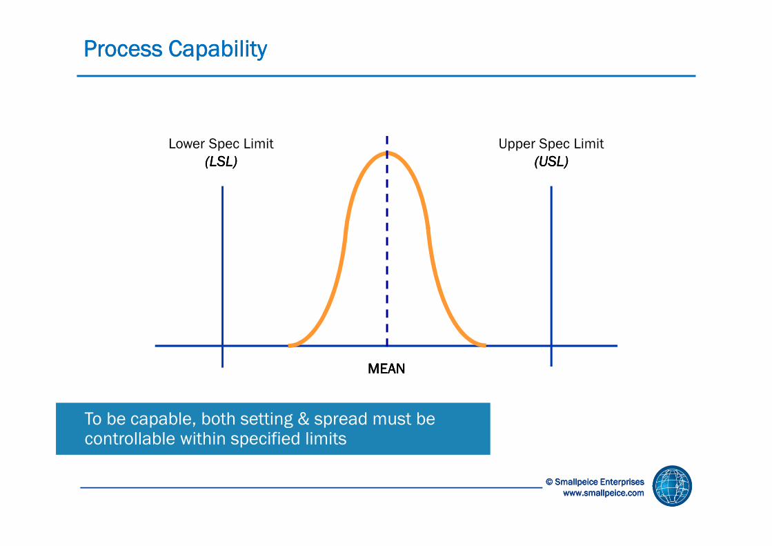
Lower Spec Limit

(LSL)(LSL)(LSL)(LSL)

Upper Spec Limit

(USL)(USL)(USL)(USL)

MEANMEANMEANMEAN

Process CapabilityProcess CapabilityProcess CapabilityProcess Capability

To be capable, both setting & spread must be controllable within specified limits



LSLLSLLSLLSL USLUSLUSLUSL

MEANMEANMEANMEAN

BEYOND BEYOND BEYOND BEYOND

SPECSPECSPECSPEC

Is this Process Capable?Is this Process Capable?Is this Process Capable?Is this Process Capable?

No! It is incorrectly set



LSL USL

MEAN

Or this One?Or this One?Or this One?Or this One?

No! It can only just meet specified requirements: there is no margin for error





A comparison of process output with specified requirements

• can the specification be met consistently?

Expressed using capability indices

• Cp & Pp - take account of process variability only

• Cpk & Ppk - also take account of process setting

• Zbench (also known as the sigma value)

Calculating Variable Data Process CapabilityCalculating Variable Data Process CapabilityCalculating Variable Data Process CapabilityCalculating Variable Data Process Capability

LSL USLX





Process capability is a key performance indicator (KPI) for Lean Sigma

projects. Process capability is assessed before, during & after the

introduction of improvements:

• Provides a ‘baseline’ measure of process performance

• Gauges effectiveness of improvements

• Monitors progress towards targets

• Provides a basis for calculating benefits

Process Capability as a KPIProcess Capability as a KPIProcess Capability as a KPIProcess Capability as a KPI





• The process is stable

• Individual measurements from the process are approximately

normally distributed

• The specification accurately reflects customer needs

• Measurement variation is small

• Acceptance that sampling variation will always exist, hence capability

indexes are not absolute, even for stable processes

Some AssumptionsSome AssumptionsSome AssumptionsSome Assumptions





• Capability can be calculated meaningfully only after special causes of

variation have been identified & eliminated.

• Ongoing control charts should ideally have been in control for

25 or more subgroups.

• For non-Normal data, more flexible techniques are required, e.g.

– graphical analysis

– computerised curve fitting

– data transformation to convert data to a Normal distribution

(last resort)

Calculating CapabilityCalculating CapabilityCalculating CapabilityCalculating Capability





Potential CapabilityPotential CapabilityPotential CapabilityPotential Capability

• Also known as ‘within’ or ‘short-term’ capability

• The theoretical capability of a process based only on within-subgroup (i.e.

common cause) variation

• Represented by capability indexes such as Cp & Cpk

Actual CapabilityActual CapabilityActual CapabilityActual Capability

• Also known as ‘overall’ or ‘long-term’ capability

• The actual capability of a process, based on total variation measured

during the period of observation

• Represented by capability indexes such as Pp & Ppk

‘Potential’ & ‘Actual’ Capability‘Potential’ & ‘Actual’ Capability‘Potential’ & ‘Actual’ Capability‘Potential’ & ‘Actual’ Capability

Let’s start by understanding Long Term capability first,

As this is consistent with the Minitab approach.





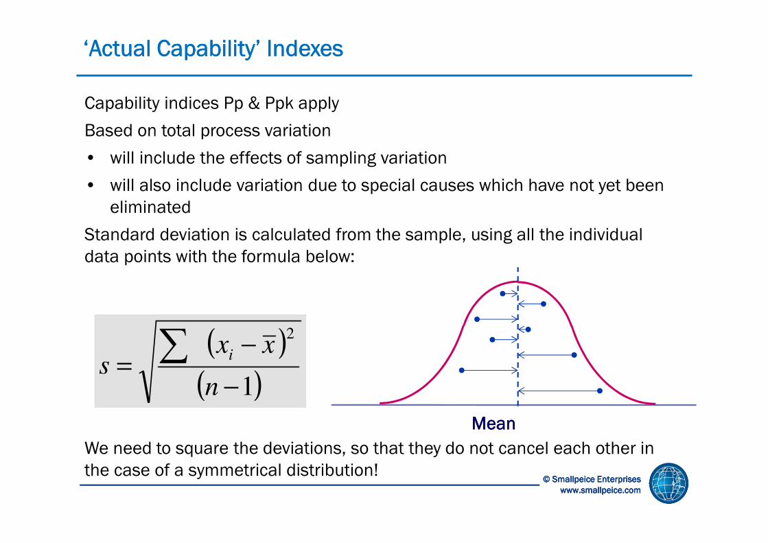
Capability indices Pp & Ppk apply

Based on total process variation

• will include the effects of sampling variation

• will also include variation due to special causes which have not yet been

eliminated

Standard deviation is calculated from the sample, using all the individual

data points with the formula below:

We need to square the deviations, so that they do not cancel each other in

the case of a symmetrical distribution!

‘Actual Capability’ Indexes‘Actual Capability’ Indexes‘Actual Capability’ Indexes‘Actual Capability’ Indexes

MeanMeanMeanMean

( )

( )1

2

−

−=

n

xxs

i





• These use similar formulae to Cp & Cpk

• The difference is in the way standard deviation is calculated

• Ppk is the lesser of PPU & PPL

Calculating PCalculating PCalculating PCalculating PPPPP & P& P& P& PPKPKPKPK IndexesIndexesIndexesIndexes

s

xUSLPPU

3

−=

s

LSLxPPL

3

−=

s6

LSLUSLPp

−−−−====





Potential capability index CCCCpppp is calculated using the formula:

USL = Upper Specification Limit

LSL = Lower Specification Limit

Absolute minimum value is 1.0

Minimum commonly set at 1.33 or 1.67

Calculating CCalculating CCalculating CCalculating CP P P P IndexIndexIndexIndex

σ̂6

LSLUSL

SpreadProcess

Tolerance SpecifiedTotalC p

−==



Calculating CCalculating CCalculating CCalculating CP P P P Index DisplayedIndex DisplayedIndex DisplayedIndex Displayed

USL

XXXX

LSL

6 σ̂

How much of the ‘potential’ estimated spread of the process could fit between the specification limits





Potential capability index CCCCpkpkpkpk is the lesserlesserlesserlesser of:

For one-sided tolerances calculate just one value, depending on whether the

upper or lower limit is specified

Like Cp, absolute minimum value is 1.0

Minimum commonly set at 1.33 or 1.67

Calculating CCalculating CCalculating CCalculating CPKPKPKPK IndexIndexIndexIndex

&σ̂3

xUSLCPU

−=

σ̂3

LSLxCPL

−=



Calculating CCalculating CCalculating CCalculating CPKPKPKPK Index DisplayedIndex DisplayedIndex DisplayedIndex Displayed

SCRAP

CPU

USLLSL

3 σ̂ 3 σ̂

XXXX

Where the ‘potential’ estimated centre of the process is in relation to the specification limits, in this case Cpu would be used





• At this stage in a Six Sigma project, baseline capability should

be determined

• Baseline capability provides a benchmark even if processes are not

yet capable

• It is likely that improvements will be iterative: it may be desirable (or

essential) to achieve effective control of contributory processes before

proceeding further

Baseline CapabilityBaseline CapabilityBaseline CapabilityBaseline Capability



Process Capability & MinitabProcess Capability & MinitabProcess Capability & MinitabProcess Capability & Minitab

Use Stat > Quality Tools > Capability Analysis > NormalUse Stat > Quality Tools > Capability Analysis > NormalUse Stat > Quality Tools > Capability Analysis > NormalUse Stat > Quality Tools > Capability Analysis > Normal



Complete the Dialogue BoxComplete the Dialogue BoxComplete the Dialogue BoxComplete the Dialogue Box

We are

analysing

‘Thickness’

Enter the

upper &

lower limits

Select ‘Options’

We will

subgroup by

‘see note’

NOTE: Sub group size determined by number or data points collected at any one time, e.g. 3 or 5.



Complete the ‘Options’ Dialogue BoxComplete the ‘Options’ Dialogue BoxComplete the ‘Options’ Dialogue BoxComplete the ‘Options’ Dialogue Box

Click ‘OK’ & ‘OK’

again

Select Percents

Select Pp

(or sigma level)’

This is where you can choose (or not) to select

the short term (within) capability estimate



Minitab Capability InformationMinitab Capability InformationMinitab Capability InformationMinitab Capability Information

Long Term

Capability

Expected Long

Term

Performance

• The ‘overall’ curve shows The ‘overall’ curve shows The ‘overall’ curve shows The ‘overall’ curve shows (greater) long term variation(greater) long term variation(greater) long term variation(greater) long term variation

• These curves are used to These curves are used to These curves are used to These curves are used to calculate the expected calculate the expected calculate the expected calculate the expected process performanceprocess performanceprocess performanceprocess performance



Minitab Capability InformationMinitab Capability InformationMinitab Capability InformationMinitab Capability Information

Display for typical

Cp,Cpk capability

indices

Expected Short

Term

Performance

• Turning on the within Turning on the within Turning on the within Turning on the within subgroup analysis adds a subgroup analysis adds a subgroup analysis adds a subgroup analysis adds a second curvesecond curvesecond curvesecond curve

• This curve predicts the This curve predicts the This curve predicts the This curve predicts the improvement achieved via improvement achieved via improvement achieved via improvement achieved via better process control.better process control.better process control.better process control.





• The process is stable: The process is stable: The process is stable: The process is stable: sigma values for unstable processes should be

treated with caution

• Individual measurements from the process are normally distributed:Individual measurements from the process are normally distributed:Individual measurements from the process are normally distributed:Individual measurements from the process are normally distributed: since

calculations are based on the normal distribution

• Measurement variation is small: Measurement variation is small: Measurement variation is small: Measurement variation is small: since capability analysis relies upon

valid data

• The specification accurately reflects customer requirements: The specification accurately reflects customer requirements: The specification accurately reflects customer requirements: The specification accurately reflects customer requirements: since

capability analysis compares process performance with the specification

Some AssumptionsSome AssumptionsSome AssumptionsSome Assumptions

EXERCISE

The image part with relationship ID rId2 was not found in the file.

Refer to Data Collection Plan Results

CASE STUDY

Case Study: Control ChartsCase Study: Control ChartsCase Study: Control ChartsCase Study: Control Charts

DNPDNPDNPDNP

• The team has been collecting data based on their data

collection plan for one month.

• Open worksheet “Data Collection Plan Results” to view the

output and input data that has been collected.

• Before we go on to establish baseline capability measures

we need to assess the stability of the process

• Use the appropriate control chart for the output data

provided in the worksheet.

• Discuss and share your conclusions about the results. Is the

process stable?

CASE STUDY

Case Study: Stability & CapabilityCase Study: Stability & CapabilityCase Study: Stability & CapabilityCase Study: Stability & Capability

• The team has been collecting data based on their data

collection plan for one month

• Open worksheet “Data Collection Plan Results” to view the

output and input data that has been collected

• Before we exit the Measure phase and go on to Analyse the

data we need to establish baseline capability measures.

• The specification limit is -6hours to 6hours

• Carry out the appropriate capability analysis for the data

provided. What is the baseline capability of the process?

DNPDNPDNPDNP

www.smallpeice.com

T. +44 (0)1926 336423


Section 5

Rolled Throughput Yield

This lesson introduces a measure of process capability

that is particularly useful for processes that have a

large number of individual steps, e.g. Assembly



InputsInputsInputsInputsAAAA

RFT = 94%RFT = 94%RFT = 94%RFT = 94%

4 reworked4 reworked4 reworked4 reworked

2 scrapped2 scrapped2 scrapped2 scrapped

BBBB

RFT = 91%RFT = 91%RFT = 91%RFT = 91%



CCCC

RFT = 92%RFT = 92%RFT = 92%RFT = 92%



OutputsOutputsOutputsOutputs9393939398989898

Rolled Throughput Yield

= RFTA x RFTB x RFTC

= 0.94 x 0.91 x 0.92

= 79%

90909090100100100100

Another Capability Metric to be aware of: Another Capability Metric to be aware of: Another Capability Metric to be aware of: Another Capability Metric to be aware of: Rolled Throughput Yield (RTY)Rolled Throughput Yield (RTY)Rolled Throughput Yield (RTY)Rolled Throughput Yield (RTY)

Process capability has a marked effect on Rolled Throughput Yield, especially with multi-stage processes...

The supervisor might

claim that this process is

running at 90% but this

doesn’t tell you the whole

story!

www.smallpeice.com

T. +44 (0)1926 336423


Section 6

Process Capability for Attribute

Data

This lesson introduces some important definitions to be

used when the data is pass/fail or count data





To calculate the Sigma value or the DPMO we can use statistical Z tables but

an easier & quicker method is to use the process capability calculator

DPMO CalculatorDPMO CalculatorDPMO CalculatorDPMO Calculator



DPMO = DPMO = DPMO = DPMO = D D D D x10x10x10x106666

N x ON x ON x ON x O

D = number of defects observedD = number of defects observedD = number of defects observedD = number of defects observed

N = number of unitsN = number of unitsN = number of unitsN = number of units

O = number of opportunities for O = number of opportunities for O = number of opportunities for O = number of opportunities for

defectsdefectsdefectsdefects

Process Capability for Discrete DataProcess Capability for Discrete DataProcess Capability for Discrete DataProcess Capability for Discrete Data

• In the previous example the % defective for the process was calculated by

comparing the distribution of the variable data against a customer

requirements & using probability to calculate the chances of a unit not

meeting the specification

• If you simply have count data (e.g. count of late invoices; count of items on a

snagging list) then you can assess how good your process is my calculating

either percentage or ‘DDDDefects PPPPer MMMMillion OOOOpportunities’

• If necessary the DPMO can then be converted to a ‘Sigma value’ using

conversion tables





For defectives:For defectives:For defectives:For defectives:

• Number of opportunities always = 1

– either something is defective, or it is not

– often applied to process outputs

For defects:For defects:For defects:For defects:

• Each defect category represents an opportunity

– focus on defects which are important to the customer & which are

likely to happen in practice

– where appropriate, group closely related defect types together, in order

to avoid overly long lists

– remain consistent throughout the project

– consider using standard definitions across the organisation

How Many ‘Opportunities’?How Many ‘Opportunities’?How Many ‘Opportunities’?How Many ‘Opportunities’?





A sample of 10 products is inspected, of which 2 are found to be defective

Sample Calculations (Defectives)Sample Calculations (Defectives)Sample Calculations (Defectives)Sample Calculations (Defectives)

D = 2D = 2D = 2D = 2 (no. of defectives observed)

N = 10 N = 10 N = 10 N = 10 (sample size)

O = 1O = 1O = 1O = 1 (no. of opportunities for defectives)

From tables: Sigma Level = 2.3Sigma Level = 2.3Sigma Level = 2.3Sigma Level = 2.3

DPMO = DPMO = DPMO = DPMO = D D D D x 10x 10x 10x 106 6 6 6 = = = = 2 2 2 2 x 1,000,000x 1,000,000x 1,000,000x 1,000,000 = 200,000 = 200,000 = 200,000 = 200,000

N x ON x ON x ON x O 10 x 110 x 110 x 110 x 1





In the same sample of 10 products, we identify a possible 7 defect

categories. On inspection a total of 6 defects are found

Sample Calculations (Defects)Sample Calculations (Defects)Sample Calculations (Defects)Sample Calculations (Defects)

D = 6D = 6D = 6D = 6 (no. of defects observed)

N = 10 N = 10 N = 10 N = 10 (sample size)

O = 7O = 7O = 7O = 7 (no. of opportunities for defects)

From tables: Sigma Level = 2.8Sigma Level = 2.8Sigma Level = 2.8Sigma Level = 2.8

DPMO = D x 1,000,000 = 6 x 1,000,000 = 85,714N x O 10 x 7

EXERCISE

Group Exercise: DPMO & SigmaGroup Exercise: DPMO & SigmaGroup Exercise: DPMO & SigmaGroup Exercise: DPMO & Sigma

THE TASKTHE TASKTHE TASKTHE TASK

referring to the information provided in the Handout 05: referring to the information provided in the Handout 05: referring to the information provided in the Handout 05: referring to the information provided in the Handout 05:

Calculate the DPMO and Sigma valuesCalculate the DPMO and Sigma valuesCalculate the DPMO and Sigma valuesCalculate the DPMO and Sigma values

‘HOW TO’ ‘HOW TO’ ‘HOW TO’ ‘HOW TO’ Instructions for working in your group:

• Elect a facilitator for your group

• Prepare your answers in word or Excel, in Zoom. in Zoom. in Zoom. in Zoom. Remember to

‘Save It’ ready for presenting back to the rest of the group.

Group EXERCISE

15 minutes

Refer to Handout 05 – DPMO & Sigma

EXERCISE

TeamTeamTeamTeam----Based Exercise: Calculating DPMO ValuesBased Exercise: Calculating DPMO ValuesBased Exercise: Calculating DPMO ValuesBased Exercise: Calculating DPMO Values

• A manufacturer of commercial cookers carries out a final

product audit on all units produced

• The following data relates to one week’s output of a

particular model

• Calculate DPMO both for the count of Defectives and for

Defects

OutputOutputOutputOutput 60 units60 units60 units60 units

Number Defective 21

Visual Defects - Casework 17

Visual Defects - Doors 5

External Labelling Defects 1

Compartment Visual Defects 2

Maneuverability Defects (Castors) 0

Paperwork Defects 1



Measure Phase Measure Phase Measure Phase Measure Phase –––– Key StepsKey StepsKey StepsKey Steps

Review SIPOC Map & prepare Current State Value Stream Map

Prepare detailed ‘As-Is’ Process Maps

Conduct a Failure Mode Effects Analysis for the current state process

Identify Waste & possible “Quick Wins”

Identify & define process output (Y) and potential process

input (X) measures

Plan data collection

Check measurement system

Collect data

Assess process control

Baseline Current Process Performance





By the end of this section you should be able to:By the end of this section you should be able to:By the end of this section you should be able to:By the end of this section you should be able to:

Section Section Section Section Objectives ReviewObjectives ReviewObjectives ReviewObjectives Review

Understand the need for Basic Statistics

Understand different types of variation

Know the anatomy & main types of control charts

Apply control charts correctly

Calculate capability for continuous data

Calculate capability for attribute data





& finally:& finally:& finally:& finally:

please complete

the online

feedback form.

Please Provide Feedback Please Provide Feedback Please Provide Feedback Please Provide Feedback

ChatChatChatChat

Click the Click the Click the Click the ChatChatChatChat icon onicon onicon onicon on

thethethethe Zoom toolbarZoom toolbarZoom toolbarZoom toolbar

Click the Click the Click the Click the

hyperlink hyperlink hyperlink hyperlink to the to the to the to the

Feedback FormFeedback FormFeedback FormFeedback Form

Complete the Complete the Complete the Complete the

FeedbackFeedbackFeedbackFeedback

Form, and Form, and Form, and Form, and

click click click click SubmitSubmitSubmitSubmit



Summary & Next StepsSummary & Next StepsSummary & Next StepsSummary & Next Steps

Recap Recap Recap Recap –––– Session ObjectivesSession ObjectivesSession ObjectivesSession Objectives

• Understand the need for Basic Stats

• Understand different types of variation

• Know the anatomy & main types of

control charts

• Apply control charts correctly

• Calculate capability for continuous data

• Calculate capability for attribute data

ACTION !ACTION !ACTION !ACTION !

• Complete the training feedback

survey in Portal

• Mark portal module as ‘complete’

• Complete knowledge test


Preparation Before Next Webinar Preparation Before Next Webinar Preparation Before Next Webinar Preparation Before Next Webinar

• Download slides from Portal

• Download supporting handouts

from Portal

• Complete any pre-work/pre-reading


For your Project WorkFor your Project WorkFor your Project WorkFor your Project Work

• Discuss how to calculate baseline

capability for your project Y with the

Process Owner

• Plan carefully and work out who else

should be involved in the study

process capability > masterclass webinar

Documents