process estimation with relay feedback · pdf fileprocess estimation with relay feedback...
TRANSCRIPT

ISSN 0280-5316 ISRN LUTFD2/TFRT--5764--SE
Process Estimation with Relay Feedback Method
Adis Kurjak Faris Mustajbasic
Department of Automatic Control Lund University February 2006


Document name MASTER THESIS Date of issue February 2006
Department of Automatic Control Lund Institute of Technology Box 118 SE-221 00 Lund Sweden Document Number
ISRNLUTFD2/TFRT--5764--SE Supervisor Tore Hägglund and Karl Johan Åström at Department of Automatic Control in Lund.
Author(s) Adis Kurjak and Faris Mustajbasic
Sponsoring organization
Title and subtitle Process Estimation with Relay Feedback Method. (Bestämning av Processmodeller från Reläexperiment)
Abstract Manual tuning of PID controllers can be very time-consuming and that is why automatic tuning was developed. The conventional automatic tuners use a relay instead of controller in a closed loop system to obtain stabile oscillations. The information from a relay experiment is later used to calculate PID control parameters with different tuning rules and there also exist systems that, apart from the relay experiment, use a step response experiment to obtain even better control. The aim with this thesis is to investigate if there is enough information in a relay experiment to estimate an unknown process as a first order process with delay and then use AMIGO design to obtain satisfying PI/PID controller parameters. The calculation of the estimation parameters of the model is done with Gauss-Newton optimization algorithm. The algorithm minimizes the square of the output error between the unknown process output and estimation model output and calculates the optimal model parameters. The algorithm is dependant of good initial Svalues so a method for initializing good values is developed.
Keywords
Classification system and/or index terms (if any)
Supplementary bibliographical information ISSN and key title 0280-5316
ISBN
Language English
Number of pages 54
Security classification
Recipient’s notes
The report may be ordered from the Department of Automatic Control or borrowed through:University Library, Box 3, SE-221 00 Lund, Sweden Fax +46 46 222 42 43


iii
Preface This master thesis is one of the requirements for the Master of Science in Electrical Engineering degree at Lund Institute of Technology (LTH) in Lund, Sweden. The quantity of this work corresponds to 40 weeks of full time work, i.e. 20 weeks per student. We would like to thank our supervisors, professor Tore Hägglund, LTH, and professor Karl Johan Åström, LTH and University of California Santa Barbara, for helping us trough this thesis and always having time when we needed help. Their hints and suggestions were very helpful when we got stuck in our work. We are grateful to the research assistant, Ph.D. Anders Robertsson at Department of Automatic Control, LTH, for helping us with the practical experiment and we would like to thank the secretaries at the Department of Automatic Control for their kindness. Last, but not the least, we would like to thank our families and our soul mates Jasmina and Amina for their support and being there for us. Lund Beginning of year 2006 Authors

iv

v
Contents Preface 1 Introduction.........................................................................................................1 2 Theory ..................................................................................................................2
2.1 PID Control................................................................................................2 2.2 Automatic Tuning of PID Controller.........................................................3 2.2.1 The Ziegler-Nichols Step Response Method ....................................3 2.2.2 The Ziegler-Nichols Closed-Loop Method.......................................4 2.2.3 Relay Feedback Method ...................................................................5 2.2.4 Describing Function Analysis...........................................................7 2.3 Amigo Design Method...............................................................................8 2.4 The Gauss-Newton Optimization Method.................................................9 2.4.1 The Newton’s Method ......................................................................9 2.4.2 The Gauss-Newton Method ............................................................10
3 Modelling of First Order Process ....................................................................12
3.1 Estimation of First Order Process............................................................12 3.2 Implementation of Estimation .................................................................15 3.3 First Order Results ...................................................................................18
4 Estimation of Higher Order Processes............................................................19
4.1 High Order Process Results .....................................................................19 4.2 Control Parameters ..................................................................................30
5 Method for the Initiation of Kp, T and L .........................................................32
5.1 Backward AMIGO Method .....................................................................32 5.2 Results of the Backwards AMIGO Method.............................................35
6 Real Process Test ..............................................................................................37
6.1 Estimation of a Tank Process...................................................................37 6.2 Control of a Tank Process........................................................................39 6.3 Comment..................................................................................................41

vi
7 Conclusions........................................................................................................42 7.1 Summary..................................................................................................42
7.2 Future Work.............................................................................................43 Appendix A...........................................................................................................44 Appendix B ...........................................................................................................45 Appendix C...........................................................................................................46 Bibliography.........................................................................................................50

1
Chapter 1
Introduction Since manual tuning of a PID controller is a very time-consuming process, automatic tuning was developed. Ziegler-Nichols tuning rules have been used for more than 50 years and today, there are several modifications of these tuning rules available. Automatic tuning is implemented in many industrial controllers, like the commercial PID controller ECA600 from ABB that uses a relay method to calculate PID-controller parameters. There are also controllers that use a step response method for this purpose. The objective of this master’s thesis is to examine if there is enough information in a relay experiment so that there is no need for additional experiments, like the step response experiment. In this way, many disadvantages with additional methods would be avoided. The basic idea is to approximate the unknown process as a first order process with delay using Gauss-Newton optimizations method and find some proper initial values for the method. The control parameters can than be obtained using AMIGO1 design method.
1 Approximate M-constrained integral gain optimization
2
Chapter 2
Theory Tuning of PID-controller parameters can be very time consuming if it is done manually. That is why automatic tuning was developed. There are several methods that can be used to auto-tune and in this chapter, the theory behind automatic tuning is treated. First, in section 2.1, PID-control is explained concisely. In section 2.2, the theory behind some simple, widely used, automatic tuning rules is explained. Section 2.3 treats the AMIGO design method and in the section 2.4 Gauss-Newton optimization method is treated.
2.1 PID Control A PID-controller is a simple controller but a very effective one. Due to the flexibility of this controller, it is the most spread controller. It is used in the majority off all applications that use automatic control where it is provided that the performance requirements are not too high [4]. The mathematical expression for the PID-controller is given by
( ) ⎟⎟⎠
⎞⎜⎜⎝
⎛++= d
iPID sT
sTKsG 11 (2.1)
where K is gain, Ti is called integral time and Td derivative time [8]. A PID controller can have serial or parallel structure. A simple parallel structure can be seen in figure 1.1.

Chapter 2. Theory
3
Figure 2.1 Parallel structure of the PID controller.
Action control of the PID-controller is based on past and present error values and prediction of future control errors, where integral part acts on the average of past errors, the proportional part acts on present error value and derivative part acts as prediction of future errors based on linear extrapolation.
2.2 Automatic Tuning of PID Controller Today, there exist several methods for tuning a PID-controller, like Ziegler-Nichols step response method and Ziegler-Nichols oscillation method. Manual tuning can be very time consuming, so it is very good and timesaving if it is done automatically and that is why automatic tuning has been introduced. Åström-Hägglund developed a method for auto tuning of PID-controllers that is related to Ziegler-Nichols oscillation method [4].
2.2.1 The Ziegler-Nichols Step Response Method
Figure 2.2 Definitions of parameters a, L, T and k in a step response experiment.
In 1942, Ziegler and Nichols published a method where the PID parameters are determined with step response data [4]. The method uses two parameters, a and L, that can be seen in figure 2.2. These parameters can be determined by looking at a maximum slope tangent of system’s step response. As figure 2.2 shows, parameter a is the difference between the value where the tangent is intercepting the

Chapter 2. Theory
4
horizontal axis and the initial value. The time difference between the time point when the step starts and the time point when the maximum slope tangent is intercepting the horizontal axis, is the time delay L. Time T in figure 2.2 is time from when delay time ends to the time point when 63% of steady state value is reached. To calculate parameter T, gain k has to be known. Relation between mentioned parameters is given by
TLka ⋅
= (2.2)
The closed loop system that is received with this method is often poorly damped and the systems with better damping can be obtained by modifying these parameters [4]. Two essential drawbacks with this method are that it is difficult to know if steady state has been reached and how large step should be applied. The step should not be so large that the production is disturbed and it should be clearly above the noise level. For example if a step is applied on a process that has large rise time, it is hard to see in a step response if it is the step response of the process that is examined or if it is, for example, play in some valves in the process. Controller parameters obtained with this method are given in table 2.1.
Parameters Type of controller
Kc Ti Td P-controller PI-controller
PID-controller
1/a 0.9/a 1.2/a
- 3L 2L
- -
L/2 Table 2.1 Controller parameters obtained with Ziegler- Nichols step response method.
2.2.2 The Ziegler-Nichols Closed-Loop Method By removing the integral and derivative part of controller we will receive pure proportional control and then by increasing the gain, oscillations of the output signal are observed. To calculate the controller gain K0 and the period time of output oscillations, T0, which this method uses in calculation of controller parameters, the gain has to be increased until stabile oscillations are observed [2]. These values of the controller gain and the period time of the output oscillation is then used to calculate controller parameter values according to the table 2.2:

Chapter 2. Theory
5
Parameters Type of controller
Kc Ti Td P-controller PI-controller
PID-controller
0.5 K0 0.45 K0 0.6 K0
- T0/1.2 T0/2
- -
T0/8 Table 2.2 Controller parameters obtained with Ziegler- Nichols frequency method.
The Ziegler-Nichols oscillation method has been used for more than 50 years although it has several drawbacks like poor robustness. One disadvantage with this method is that, when getting the parameters Kc, Ti and Td, one has to work with the closed loop system on the stability boundary with the risk of having uncontrollable oscillations that can harm the process. To avoid this, Åström-Hägglund developed so called relay experiment method where the controller is replaced by a relay. Since a relay has a limited output, stabile oscillations are obtained [2].
2.2.3 Relay Feedback Method To avoid the requirements, that when calculating controller parameter values with Ziegler-Nichols oscillation method, one has to work on the stability boarder with risk of having unstable oscillations, a relay method has been developed by Åström and Hägglund. In this method, a PID controller is replaced with a relay and stabile and controllable oscillations are obtained, see figure 2.3 [4, 7].
Figure 2.3 Schematics of a relay experiment.
The relay works in this case as a constant gain that gives constant oscillations independent of the input signal, i.e. the amplitude and frequency in the output from the relay, a square wave, is determined by the relay’s hysteresis and its output level. An example of relay output signal and the process output can be seen in figure 2.5. If relay has no hysteresis, the working point will be on the
Chapter 2. Theory
6
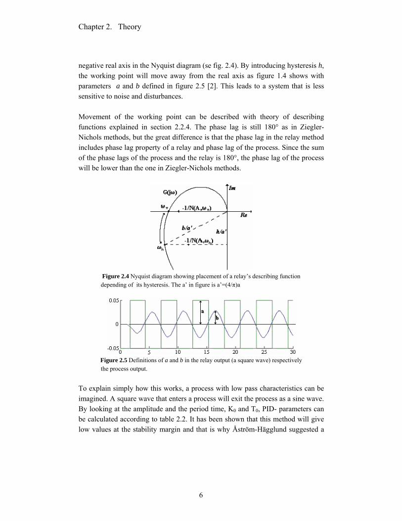
negative real axis in the Nyquist diagram (se fig. 2.4). By introducing hysteresis h, the working point will move away from the real axis as figure 1.4 shows with parameters a and b defined in figure 2.5 [2]. This leads to a system that is less sensitive to noise and disturbances. Movement of the working point can be described with theory of describing functions explained in section 2.2.4. The phase lag is still 180° as in Ziegler-Nichols methods, but the great difference is that the phase lag in the relay method includes phase lag property of a relay and phase lag of the process. Since the sum of the phase lags of the process and the relay is 180°, the phase lag of the process will be lower than the one in Ziegler-Nichols methods.
Figure 2.4 Nyquist diagram showing placement of a relay’s describing function depending of its hysteresis. The a’ in figure is a’=(4/π)a
Figure 2.5 Definitions of a and b in the relay output (a square wave) respectively the process output.
To explain simply how this works, a process with low pass characteristics can be imagined. A square wave that enters a process will exit the process as a sine wave. By looking at the amplitude and the period time, K0 and T0, PID- parameters can be calculated according to table 2.2. It has been shown that this method will give low values at the stability margin and that is why Åström-Hägglund suggested a

Chapter 2. Theory
7
modification of table 2.2, more than fifteen years ago. uc KK 35.0= ,
ui TT 77.0= and ud TT 19.0= were suggested as new PID parameters [2].
2.2.4 Describing Function Analysis Describing function analysis is a method that can be used to predict and approximately analyze nonlinear behaviour. The basic idea is to approximate a nonlinearity by a linear equivalent and then use different frequency domain techniques to analyze the resulting system [3]. Since a relay is a nonlinearity, this analysis is used.
Figure 2.6 Relay feedback circuit.
Signal ( )tu in figure 2.6 can be written as ( ) ( ) ( )xANtu −⋅= ω, where ( )ω,AN is a frequency response function of the relay, also called a describing function that is amplitude and frequency dependant. A relay’s describing function without hysteresis is given by
( )baAN⋅⋅
=π
ω 4, , (2.3)
where a and b are defined in figure 2.5. If hysteresis h is introduced in a relay, the describing function is than given by
( ) ⎟⎟
⎠
⎞
⎜⎜
⎝
⎛−⎟
⎠⎞
⎜⎝⎛−=
bhi
bh
baAN
2
14,π
ω . (2.4)
If it is assumed that the reference value is zero and that there are oscillations with amplitude A and frequency uω in the system, output ( )ty can be written as
( ) ( )uu jGANey ωω ⋅⋅= ,

Chapter 2. Theory
8
and with the reference value set to zero, this can be rewritten as
( ) ( )uu jGANyy ωω ⋅⋅−= ,
which gives
( ) ( ) ( ) ( )uuuu AN
jGjGANω
ωωω,
11, −=⇔−=⋅ (2.5)
This means that the intersections between ( )ujG ω and ( )uAN ω,1
− gives the
ultimate frequency, uω , and amplitude, A , for the oscillation. Absolute value of
( )ujG ω is called ultimate gain and can be written, using a relay’s describing
function, as abKu ⋅⋅
=4π [3, 6].
2.3 Amigo Design Method Instead of using two parameters to calculate controller parameters as in Ziegler- Nichols methods, there is a method called AMIGO, proposed in [5], that uses three parameters Kp, T and L that correspond to the parameters of a first order model with time delay
( ) ( )sUsT
eKsYsL
pm +=
−
1.
The AMIGO method suggests that the controller parameters for a PI-controller should be calculated as follow:
( )
22
2
2
7121335.0
35.015.0
LLTTLTLT
LKT
TLLT
KK
i
ppc
+++=
⎟⎟⎠
⎞⎜⎜⎝
⎛
+−+=
(2.6)
PID controller parameters are calculated in the following way:

Chapter 2. Theory
9
TLLTT
LTL
TLT
LT
KK
d
i
pc
+=
++
=
⎟⎠⎞
⎜⎝⎛ +=
3.05.0
1.08.04.0
45.02.01
(2.7)
AMIGO design method will not be described in detail in this master thesis. For those interested in AMIGO, a detailed description can be found in [5].
2.4 The Gauss-Newton Optimization Method Today, there exist many optimization methods that are used to find a minimum of a function of several variables. Multi-dimensional optimization is difficult because several local minima may exist and neither of them might be a global one. It is only in simple cases that it is possible to determine minimum exactly and that is why one has to resort to numerical methods. These numerical methods consist of some scheme for wandering around in the domain of the function to be minimized, and trying to find smaller and smaller function values [1]. There is no general optimization method that will solve all problems because most of the methods are designed to work in certain applications and might be useless in other applications. Since one of our problems is to minimize a loss function given by a quadratic function, a modified Newton’s method, so called the Gauss Newton method is suggested for this kind of problems. That is why this method has been chosen, described and implemented in this master thesis.
2.4.1 The Newton’s Method Assume that the function of n variables f is a class C2. Then, by Taylor’s formula, near a point xk, we can approximate f(x) by the quadratic function

Chapter 2. Theory
10
( ) ( ) ( ) ( ) ( ) ( )( )kkT
kkT
kk xxxHxxxxxfxfxq −−+−∇+=21 (2.8)
where ( )kxH denotes the Hessian of f at xk. If this matrix is positive definite, this
Taylor expansion has a minimum where ( ) 0=∇ xq . By differentiation of q we obtain
( ) 0=∇ xq ⇔
( ) ( )( ) 0=−+∇ kkk xxxHxf ⇔
( ) ( )kkk xfxHxx ∇−= −1
This formula is used as a basis for an iteration step since xk is supposed to be close to a minimum point x of function f. This means that the iteration formula is given by
( ) ( )kkkk xfxHxx ∇−= −+
11 (2.9)
The iteration of this formula starting from some initial point is defined as Newton’s method with search direction
( ) ( )kkk xfxHd ∇−= −1 (2.10)
where the unit step is taken in that direction [1]. It is possible to calculate better step lengths in every iteration step, called line search, which could give better convergence of function variables but this will not be treated here.
2.4.2 The Gauss-Newton Method The Gauss- Newton method is based on the Newton’s method applied to a least squares problem with an approximation. If there is a function f in a sum of squares
( ) ( )( )∑=
=m
ii xrxf
1
2 ∈x R

Chapter 2. Theory
11
then the differentiation of f is given by
( ) ( ) ( )∑=
∇=∇m
iii xrxrxf
12 .
By introducing the Jacobian of ( )Tmrrr ,,1 K= , i.e. the nm× -matrix
( ) ⎟⎟⎠
⎞⎜⎜⎝
⎛∂∂
=k
i
xrxJ , this can be written as
( ) ( ) ( )xrxJxf T2=∇ . Hessian of f is given by
( ) ( ) ( ) ( ) ( )∑=
∇+=m
iii
T xrxrxJxJxH1
222 (2.11)
By assuming, by the nature of the problem, that all ( )xri are close to zero or not to
large near the minimum, following approximation can be made
( ) ( ) ( )xJxJxH T2≈ . (2.12) This modification of Newton’s method is called Gauss-Newton’s method. With this approximation it is now only necessary to calculate first derivatives of ir .
The iteration scheme for this method is given by
( ) ( ) ( )kT
kkkk xrxJxHxx 11
−+ −= (2.13)
For the convergence of this method, it is required that the initial point is sufficiently near the minimum and also that the neglected terms in Hessian are small enough. Line search can also be used in this method by multiplying direction
( ) ( ) ( )kT
kkk xrxJxHd 1−−= (2.14)
with step length kλ that is calculated with line search at every iteration step [1].

12
Chapter 3
Modelling of First Order Process To receive good controller parameters based on AMIGO-design method, the process to be controlled is estimated as a first order process and parameters K, T and L are calculated. Section 3.1 describes how Gauss-Newton method is used to calculate K, T and L. In the section 3.2, the implementation of estimation of first order process is treated. Finally, a result that proves that the implementation works is presented in section 3.3.
3.1 Estimation of First Order Process To estimate higher order process as a first order process with time delay, a model in Matlab was developed using Gauss-Newton minimization method. The first order model, i.e. the estimation of higher order models, is given by
( ) ( )sUsT
eKsYsL
pm +=
−
1
where Kp is gain, L is time delay and T is time constant. Estimation of an unknown process, as a first order process is done by minimizing a loss function given by
( ) ( )( )∫ −=T
m dttytyJ0
2
21

Chapter 3. Modelling of First Order Process
13
where y(t) is the process output and ym(t) is the output from the estimated process model. This means that the error between model output and process output is minimized. The structure for Gauss-Newton algorithm for minimizing the loss function is made in the following order:
1. Starting guessing parameters pK ,T and L , i.e. .
2. Calculating J , θ∂∂J and 2
2
θ∂∂ J .
3. Updating the value of θ
where [ ]TLTK=θ . First, a function evaluation has to be done and then, the gradients are used for minimizing the loss function. A general expression for the loss function can be written as
( ) ( ) ( )( )∫ −=T
m dttytyJ0
2
21θ .
The derivative of J with respect to θ is then calculated with the following expression:
( ) ( )( ) ( )dt
tytytyJ T
mm∫ ⎟
⎠⎞
⎜⎝⎛
∂∂
−−=∂∂
0 θθ
where the derivatives ( )θ∂
∂ tym with respect to pK ,T and L in s-plane are
( ) ( ) ( )
( )( )
( ) ( )
( ) ( ) ( )ssYsUesT
sKL
sY
sYsT
ssUesT
sKT
sY
sYK
sUesTK
sY
msLpm
msLpm
mp
sL
p
m
−=⋅+
⋅−=
∂∂
+−=⋅
+
⋅−=
∂∂
=⋅+
=∂∂
−
−
−
1
11
11
1
2

Chapter 3. Modelling of First Order Process
14
Every step in the minimization of the loss function J includes new calculations of θ∂∂J and 22 θ∂∂ J with value on θ , where θ is calculated in an update law.
The update law is obtained from the Taylor expression of J with some initial value 0θ onθ :
( ) ( ) ( ) ( )02
2
000 21 θθ
θθθθθ
θθ −
∂∂
−+−∂∂
+=JJJJ T
T
(3.1)
( ) 002
2
=−∂∂
+∂∂ θθ
θθJJ T
This can be written as an update law for θ where kθ is 0θ in the first step:
⎟⎟⎠
⎞⎜⎜⎝
⎛∂∂
⎟⎟⎠
⎞⎜⎜⎝
⎛
∂∂
−=−
+k
T
kkk
JJθθ
θθ1
2
2
1 (3.2)
The second derivative that is included in the update law is given by
( ) ( )( ) ∫ ∫∫ ≥⎟⎠⎞
⎜⎝⎛∂∂
≈⎟⎠⎞
⎜⎝⎛∂∂
⎟⎠⎞
⎜⎝⎛∂∂
+⎟⎟⎠
⎞⎜⎜⎝
⎛∂∂
−−=∂∂ 0
0
2
20
2
2
2
2 Tm
Tmm
Tm
m dty
dtyy
dty
tytyJθθθθθ
where ( ) ( )( )tyty m− in the expression goes towards zero and thus can be
neglected according to Gauss Newton algorithm. Hence the approximation can be made. Since ( ) LsYm ∂∂ has a factor s in its expression, it is hard to implement it in the
MATLAB® since MATLAB®’s Simulink has no block that supports functions with only zeros and no poles. To make the implementation of θ∂∂J in MATLAB® easy, the expression of it is made in state space form. Two state variables x1 and x2 are introduced as

Chapter 3. Modelling of First Order Process
15
( ) dp
dp
UsT
Kx
UsT
Kx
22
1
1
1
+=
+=
(3.3)
where d
sLd UeU −=
This now gives a system in the state space form:
( ) ( )
( ) ( )212
12
11
1
11
11
xxTdt
dxxxsT
uKxTdt
dxUKxsT dpdp
−=⇒=+
+−=⇒⋅=+
With this state space expression, pKJ ∂∂ , TJ ∂∂ and LJ ∂∂ can be rewritten in a
way that makes it easy to implement in Simulink.
( )
( )dpm
m
pp
m
uKxTdt
dxL
Y
xxTdt
dxTY
xKK
Y
+−−=−=∂∂
−−=−=∂∂
=∂∂
11
212
1
1
1
1
3.2 Implementation of Estimation The implementation of the estimation model is implemented, as mentioned earlier, in MATLAB® and its Simulink that is a software package for modeling, simulating and analyzing dynamical systems. To make it easy to verify that the program works properly, we started by estimating a first order process where parameters pK ,T and L are initiated by us, i.e. are known. Major part of the
program is implemented in Simulink where the first and second derivatives of the loss function are calculated. The Simulink model is executed by an m-file where

Chapter 3. Modelling of First Order Process
16
the update law is implemented. The schema of the implementation can be seen in figure 3.1.
Figure 3.1 Schematics of implementation of estimation
When the new values of pK ,T and L are calculated, they are used as new values
in Simulink model. This can be done while the difference between current parameters and the parameters calculated in the step before exceeds some value initiated by the user. It can also be done in a finite number of steps as it is done in this master thesis where the algorithm is repeated 8 times. The reason why the first alternative was discarded is that it can take very long time until the difference between the parameters gets below the initiated value. The simulation time is chosen by looking at the signals in a relay experiment and chose the time when 4 periods of process output oscillation have occurred. The m-files and the Simulink model with its subsystems can be seen in Appendix A, B and C. Since we know the values of the process parameters, it is easy to verify that the estimation works, simply by comparing the calculated values and process values. After countless executions of the program, we realized how important the initial values are. It was important to find good values, especially for the parameter L. To find these values, we first had to make a Simulink model that was a pure relay experiment. To calculate good initial values with help of the model, we followed a few rules that follows. The initial gain K could easily be determined simply by looking at the relation between the process output and input. This gain corresponds to gain when the phase is 180°, i.e. it is smaller than the static gain. If ( )sG is given by
( )sT
eKsGsL
p +=
−
1,

Chapter 3. Modelling of First Order Process
17
then the absolute value of ( )sG is
221 T
KG p
ω+= .
Finally, with equation (2.5), following expression is obtained for initial Kp,
ab
T
KK p
⋅⋅
=+
=41 22
π
ω.
To determine the time constant T a step was used as an input to our system and the rise time was examined and used as an initial value. Determination of the time delay L is more complicated. To determine an initial value of L, the relation between time delay and time period Tp was investigated. This relation can be expressed in following way with argument of the transfer function ( )sG :
- ( ) πωωω =+= TLiG 000 arctanarg
To determine the interval where parameter L is assumed to have a value, and with facts that 00 ≥Tω , i.e that ( ) 2arctan0 0 πω ≤≤ T , two cases are studied.
pp TTLL21
200 ===⇔=
ππ
ωππω
pp TTLL41
222
2 00 ===⇔=+
ππ
ωπππω
which gives the interval for L as
pp TLT21
41
≤≤ .

Chapter 3. Modelling of First Order Process
18
This parameter initialization method was done only to verify that the program works correctly and it is not a general method for finding initial values. In this case a step response of the process was investigated to find T and the goal with this thesis is to avoid step response experiments. That is why other methods for finding initial values had to be found.
3.3 First Order Results
Process Parameters Initial value Final value K 1.5 2.000 T 3.5 4.000
sp e
sG 2
)41(2 −
+=
L 2.6 1.998
Figure 3.2 Bode and Nyquist plot showing the “unknown” process and the
first order estimation.
Figure 3.3 Open loop step response of the “unknown” process and its first order estimation.
The figures 3.2 and 3.3 show how good estimation of a first order process is obtained. The parameters in the first order process are estimated successfully. The initial values for the optimization algorithm were calculated with rules presented in section 3.2.

19
Chapter 4
Estimation of Higher Order Processes This chapter presents the results that confirm the functionality of the implemented process estimator for higher order processes. In section 4.1, the results of the estimation are presented in different plots together with PI- and PID control. In section 4.2, the calculated values of the controller parameters are presented and compared with ones of the step response method.
4.1 High Order Process Results Since the program for estimation of the first order process worked as wished, the next step was to use the program for estimation of higher order processes. Representing ten different processes, the initial values of parameters for the optimization algorithm were obtained from the Department of Automatic Control in Lund. These values were used at the department to calculate the controller parameters, but in our case, they were used only as initial values since it was assumed that they were not far from the optimal values. This was done to affirm that the Gauss-Newton method works even for more complicated processes and gives acceptable values of the parameters K, T and L. Applied to AMIGO design rules, these parameters are expected to give a good control. In the following plots, a wide range of processes of different order are estimated and compared with the estimation. The PI- and PID control of every process is also investigated and compared to control obtained with the values that were used as initial values in the Gauss-Newton method, i.e. the values from the department.
Chapter 4. Estimation of Higher Order Process
20
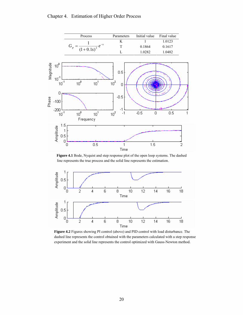
Process Parameters Initial value Final value K 1 1.0123 T 0.1864 0.1617
sp e
sG −
+= 2)1.01(
1
L 1.0282 1.0482
Figure 4.1 Bode, Nyquist and step response plot of the open loop systems. The dashed
line represents the true process and the solid line represents the estimation.
Figure 4.2 Figures showing PI control (above) and PID control with load disturbance. The dashed line represents the control obtained with the parameters calculated with a step response experiment and the solid line represents the control optimized with Gauss-Newton method.

Chapter 4. Estimation of Higher Order Process
21
Process Parameters Initial value Final value K 1 1.3507 T 1.8643 2.6754
sp e
sG −
+= 2)1(
1
L 1.2817 1.3732
Figure 4.3 Bode, Nyquist and step response plot of the open loop systems. The dashed
line represents the true process and the solid line represents the estimation.
Figure 4.4 Figures showing PI control (above) and PID control with load disturbance. The dashed line represents the control obtained with the parameters calculated with a step response experiment and the solid line represents the control optimized with Gauss-Newton method.
.
Chapter 4. Estimation of Higher Order Process
22
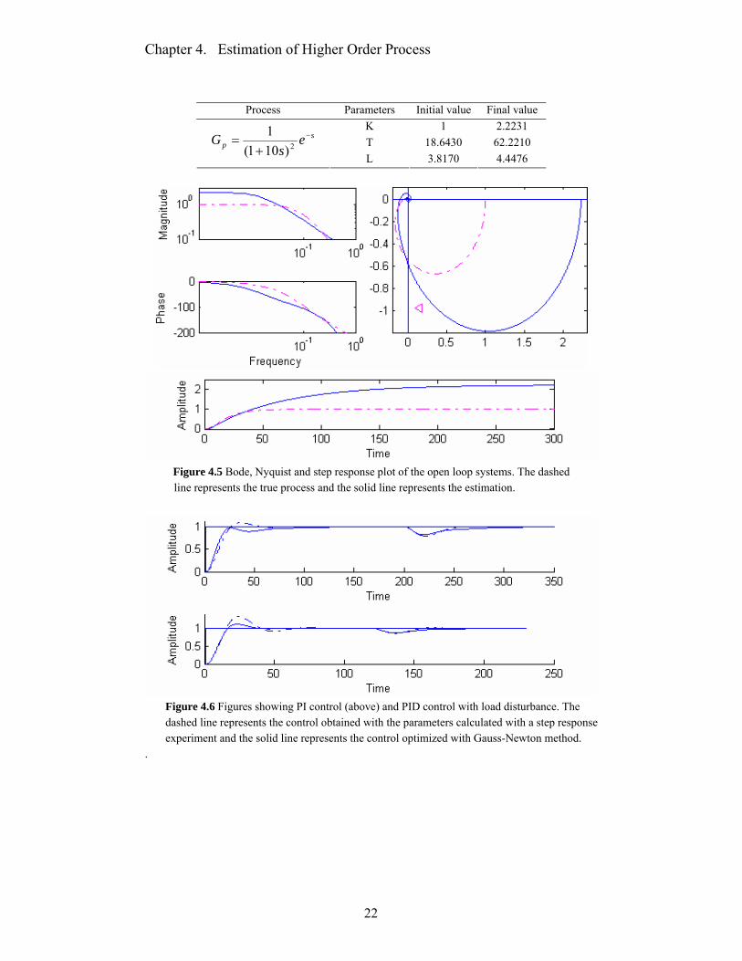
Process Parameters Initial value Final value K 1 2.2231 T 18.6430 62.2210
sp e
sG −
+= 2)101(
1
L 3.8170 4.4476
Figure 4.5 Bode, Nyquist and step response plot of the open loop systems. The dashed
line represents the true process and the solid line represents the estimation.
Figure 4.6 Figures showing PI control (above) and PID control with load disturbance. The dashed line represents the control obtained with the parameters calculated with a step response experiment and the solid line represents the control optimized with Gauss-Newton method.
.

Chapter 4. Estimation of Higher Order Process
23
Process Parameters Initial value Final value K 1 1.4223 T 1.04 1.8551 ( )( )( )ssss
Gp 32 1.011.011.01)1(1
++++=
L 0.075 0.0852
Figure 4.7 Bode, Nyquist and step response plot of the open loop systems. The dashed
line represents the true process and the solid line represents the estimation.
Figure 4.8 Figures showing PI control (above) and PID control with load disturbance. The dashed line represents the control obtained with the parameters calculated with a step response experiment and the solid line represents the control optimized with Gauss-Newton method.
.

Chapter 4. Estimation of Higher Order Process
24
Process Parameters Initial value Final value K 1 1.6887 T 1.48 3.3363 ( )( )( )ssss
Gp 32 5.015.015.01)1(1
++++=
L 0.5 0.5912
Figure 4.9 Bode, Nyquist and step response plot of the open loop systems. The dashed
line represents the true process and the solid line represents the estimation.
Figure 4.10 Figures showing PI control (above) and PID control with load disturbance. The dashed line represents the control obtained with the parameters calculated with a step response experiment and the solid line represents the control optimized with Gauss-Newton method.
Chapter 4. Estimation of Higher Order Process
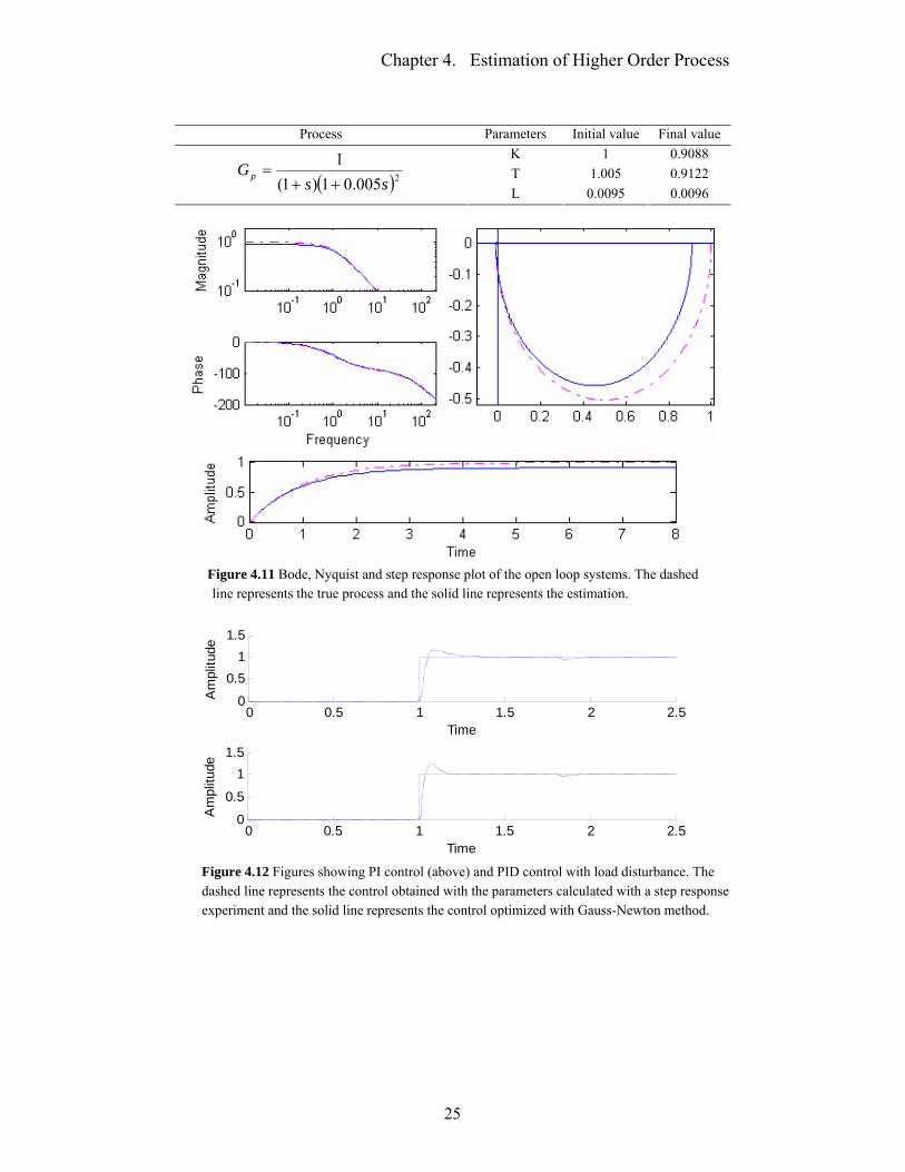
25
Process Parameters Initial value Final value K 1 0.9088 T 1.005 0.9122 ( )2005.01)1(
1ss
Gp++
=
L 0.0095 0.0096
Figure 4.11 Bode, Nyquist and step response plot of the open loop systems. The dashed
line represents the true process and the solid line represents the estimation.
0 0.5 1 1.5 2 2.50
0.51
1.5
Time
Am
plitu
de
0 0.5 1 1.5 2 2.50
0.5
11.5
Time
Am
plitu
de
Figure 4.12 Figures showing PI control (above) and PID control with load disturbance. The dashed line represents the control obtained with the parameters calculated with a step response experiment and the solid line represents the control optimized with Gauss-Newton method.

Chapter 4. Estimation of Higher Order Process
26
Process Parameters Initial value Final value K 3 1.4726 T 1.0662 2.0099 ( )21.01)1(
1ss
Gp++
=
L 0.1445 0.1598
Figure 4.13 Bode, Nyquist and step response plot of the open loop systems. The dashed
line represents the true process and the solid line represents the estimation.
Figure 4.14 Figures showing PI control (above) and PID control with load disturbance. The dashed line represents the control obtained with the parameters calculated with a step response experiment and the solid line represents the control optimized with Gauss-Newton method.

Chapter 4. Estimation of Higher Order Process
27
Process Parameters Initial value Final value K 1 0.7726 T 18.717 21.9609 ( )2101)1(
1ss
Gp++
=
L 3.7716 4.4933
Figure 4.15 Bode, Nyquist and step response plot of the open loop systems. The dashed
line represents the true process and the solid line represents the estimation.
Figure 4.16 Figures showing PI control (above) and PID control with load disturbance. The dashed line represents the control obtained with the parameters calculated with a step response experiment and the solid line represents the control optimized with Gauss-Newton method.

Chapter 4. Estimation of Higher Order Process
28
Process Parameters Initial value Final value K 1 1.5222 T 1.4250 5.4915 ( )41
1s
Gp+
= L 1.6292 1.6970
Figure 4.17 Bode, Nyquist and step response plot of the open loop systems. The dashed
line represents the true process and the solid line represents the estimation.
Figure 4.18 Figures showing PI control (above) and PID control with load disturbance. The dashed line represents the control obtained with the parameters calculated with a step response experiment and the solid line represents the control optimized with Gauss-Newton method.
.

Chapter 4. Estimation of Higher Order Process
29
Process Parameters Initial value Final value K 1 1.4307 T 4.3300 6.1636 ( )81
1s
Gp+
= L 4.3100 4.6453
Figure 4.19 Bode, Nyquist and step response plot of the open loop systems. The dashed
line represents the true process and the solid line represents the estimation.
Figure 4.20 Figures showing PI control (above) and PID control with load disturbance. The dashed line represents the control obtained with the parameters calculated with a step response experiment and the solid line represents the control optimized with Gauss-Newton method.
Chapter 4. Estimation of Higher Order Process
30
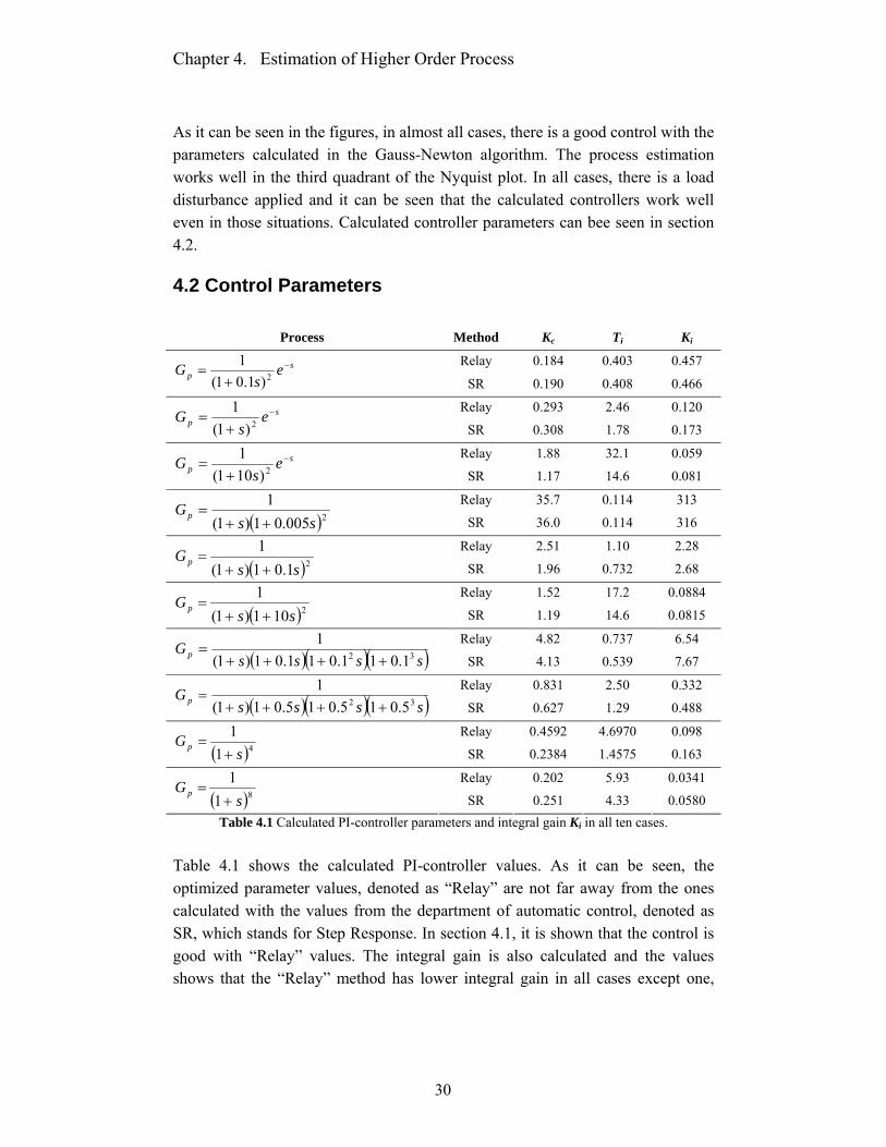
As it can be seen in the figures, in almost all cases, there is a good control with the parameters calculated in the Gauss-Newton algorithm. The process estimation works well in the third quadrant of the Nyquist plot. In all cases, there is a load disturbance applied and it can be seen that the calculated controllers work well even in those situations. Calculated controller parameters can bee seen in section 4.2.
4.2 Control Parameters
Process Method Kc Ti Ki
Relay 0.184 0.403 0.457 sp e
sG −
+= 2)1.01(
1 SR 0.190 0.408 0.466
Relay 0.293 2.46 0.120 sp e
sG −
+= 2)1(
1 SR 0.308 1.78 0.173
Relay 1.88 32.1 0.059 sp e
sG −
+= 2)101(
1 SR 1.17 14.6 0.081
Relay 35.7 0.114 313
( )2005.01)1(1
ssGp
++=
SR 36.0 0.114 316
Relay 2.51 1.10 2.28
( )21.01)1(1
ssGp
++=
SR 1.96 0.732 2.68
Relay 1.52 17.2 0.0884
( )2101)1(1
ssGp
++=
SR 1.19 14.6 0.0815
Relay 4.82 0.737 6.54
( )( )( )ssssG p 32 1.011.011.01)1(
1++++
=SR 4.13 0.539 7.67
Relay 0.831 2.50 0.332
( )( )( )ssssG p 32 5.015.015.01)1(
1++++
=SR 0.627 1.29 0.488
Relay 0.4592 4.6970 0.098
( )411s
G p+
= SR 0.2384 1.4575 0.163
Relay 0.202 5.93 0.0341
( )811s
G p+
= SR 0.251 4.33 0.0580
Table 4.1 Calculated PI-controller parameters and integral gain Ki in all ten cases. Table 4.1 shows the calculated PI-controller values. As it can be seen, the optimized parameter values, denoted as “Relay” are not far away from the ones calculated with the values from the department of automatic control, denoted as SR, which stands for Step Response. In section 4.1, it is shown that the control is good with “Relay” values. The integral gain is also calculated and the values shows that the “Relay” method has lower integral gain in all cases except one,

Chapter 4. Estimation of Higher Order Process
31
but they are close to the values of the SR-method. This confirms that the control obtained with the values optimized in Gauss-Newton algorithm is satisfying. The values for the PID controller can be seen in table 4.2.
Process Method Kc Ti Td Ki
Relay 0.2661 0.5403 0.1780 0.493 sp e
sG −
+= 2)1.01(
1 SR 0.2816 0.5504 0.1936 0.513
Relay 0.797 2.25 0.600 0.354 sp e
sG −
+= 2)1(
1 SR 0.855 1.75 0.531 0.489
Relay 2.9218 21.4907 2.1771 0.136 sp e
sG −
+= 2)101(
1 SR 2.3979 11.0461 1.7981 0.216
Relay 47.2704 0.0699 0.0048 676
( )2005.01)1(1
ssGp
++=
SR 47.5921 0.0697 0.0047 680
Relay 3.98 0.741 0.0780 5.37
( )21.01)1(1
ssGp
++=
SR 3.52 0.524 0.0694 6.72
Relay 3.12 13.0 2.12 0.239
( )2101)1(1
ssGp
++=
SR 2.43 11.0 1.78 0.221
Relay 7.0295 0.4778 0.0420 14.7
( )( )( )ssssG p 32 1.011.011.01)1(
1++++
=SR 6.4400 0.3612 0.0367 17.8
Relay 1.62 1.86 0.281 0.871
( )( )( )ssssG p 32 5.015.015.01)1(
1++++
=SR 1.53 1.07 0.227 1.43
Relay 1.09 3.83 0.777 0.285
( )411s
G p+
= SR 0.594 1.65 0.607 0.360
Relay 0.557 5.99 1.89 0.0930
( )811s
G p+
= SR 0.652 4.71 1.66 0.138
Table 4.2 Calculated PID-controller parameters and integral gain Ki in all ten cases. As it can be seen in table 4.2, the same results are obtained with PID control as in PI control. In all cases except for one, when the sixth process from above is estimated, the integral gain is lower. This means that the area between the reference value and the process output is higher, i.e. the same result is obtained as in the case with the PI-control.
32
Chapter 5
Method for the Initiation of Kp, T and L The method of initialization of parameters Kp, T and L, in this master thesis referred as backward AMIGO is presented in section 5.1. In section 5.2, the results of PID control received with parameters calculated with method presented in 5.1 is compared with control obtained with the step response method.
5.1 Backward AMIGO Method As mentioned in chapter 3.2 and shown in chapter 4, the Gauss-Newton’s method needs good initial values of parameters Kp, T and L. For this reason, it is important to find a method that gives satisfying initial parameters in the general case. These three parameters have to be obtained from a simple relay experiment by looking at interesting parts of the input and output signal. The delay parameter L was assumed to be a critical parameter, since it was noticed in previous tests that it was important to have a very good approximation of it. A small change in the value of L could lead to completely different results. By investigating relay experiment signals from all tested processes in chapter 4 and looking at obtained approximated values of L in those tests, it was noticed that a very good approximation of L can be obtained directly from a relay experiment as figure 5.1 shows.

Chapter 5. Method for the Initiation of KP, T and L
33
Figure 5.1 Approximation of the parameter L in the relay experiment
The parameters Kp and T could not be obtained in same way as the parameter L. Because of that, a method for finding these parameters was developed. The Ziegler-Nichols frequency method gives fairly satisfying controller parameters. Since the Gauss-Newton method needs fairly good initial values that converge to optimal parameters, it is assumed that the controller parameters obtained with these optimal parameters will be relatively near to the parameters obtained with Ziegler-Nichols frequency method. The idea is to use fairly good controller parameters and then go backwards in AMIGO design rules to obtain initial values for the optimization algorithm. By rewritting the AMIGO rules (2.7) for PID controller with respect to the process parameters, following relations are calculated:
⎟⎠⎞
⎜⎝⎛ +=
−⋅⋅⋅
=
⋅⋅−⎟⎠⎞
⎜⎝⎛ ⋅+⋅
−⋅+⋅
=
LT
KK
TLLT
T
TTTTTT
L
cp
d
d
iddidi
45.02.015.03.0
85.42
8.05.22
8.05.2 2
(5.1)
By using the Ziegler-Nichols frequency method, parameters Kc, Ti and Td are calculated and applied to (5.1) to obtain initial values of Kp, T. Notice that L in (5.1) is only used in calculation of K and T and is not used as initial value since good initial value of it is obtained as mentioned earlier. Instead of using Ziegler-Nichols method and its modification to find a fairly good controller for the backward AMIGO, another method could be used as proposed in [5]. Following relations are suggested:

Chapter 5. Method for the Initiation of KP, T and L
34
( )180
180
180
4
95.01115.0
216.0
1.03.0
TT
TT
KK
d
i
c
κκ
κ
κ
−−
=
+=
−=
(5.2)
where κ is the gain ratio between 180K and cK .
Figure 5.2 Controller parameters as a function of gain ratio κ
The gain ratio is chosen in figure (5.2) where the upper right plot shows 180KKc
vs κ . As it can bee seen, there is a linear region up to 4.0≈κ and this inserted in (5.2) leads to following relations:
ud
ui
uc
TTTTKK
14.033.03.0
===
(5.3)
To avoid imaginary values in the expression for the parameter L in (5.1), the factor of 0.33 in (5.3) was set a little higher. The expression of Kc was also changed a little bit to get higher values of it so the value of K in (5.1) decreases little. The new values are

Chapter 5. Method for the Initiation of KP, T and L
35
ud
ui
uc
TTTT
KK
14.04.035.0
===
(5.4)
In this master thesis, these rules are used to calculate new parameters for the backward AMIGO since it was noticed that the Zigler-Nichols method gave poor initial values.
5.2 Results of the Backwards AMIGO Method The results showing the values obtained with help of backward AMIGO method are presented in table 5.1
Process Parameter Kp T L
Initial - - - sp e
sG −
+= 2)1.01(
1 Final - - -
Initial 4.33 1.92 1.15 sp e
sG −
+= 2)1(
1 Final 1.35 2.67 1.38
Initial 13.0 9.71 4.57 sp e
sG −
+= 2)101(
1 Final 1.74 48.57 4.61
Initial 23.16 0.161 0.0098
( )2005.01)1(1
ssGp
++=
Final 0.84 0.85 0.0097
Initial 14.33 0.403 0.138
( )21.01)1(1
ssG p
++=
Final 1.18 1.61 0.165
Initial 12.41 9.91 3.95
( )2101)1(1
ssG p
++=
Final 1.63 47.0 4.38
Initial 18.46 0.292 0.0669
( )( )( )ssssG p 32 1.011.011.01)1(
1++++
=Final 1.35 1.76 0.0854
Initial 8.05 1.05 0.488
( )( )( )ssssG p 32 5.015.015.01)1(
1++++
=Final 2.06 4.09 0.576
Initial 5.85 2.66 1.60
( )411s
G p+
= Final 1.57 5.67 1.71
Initial 3.34 5.88 3.87
( )811s
G p+
= Final 1.30 5.54 4.67
Table 5.1 Ten process estimations made with the backward AMIGO method. The table 5.1 shows that the initial values are not so close to the final values but the algorithm generates very good values that are close to the values in section

Chapter 5. Method for the Initiation of KP, T and L
36
4.1. As it is mentioned earlier, good initial values are necessary in the Gauss-Newton algorithm. The explanation to the large difference between the values can be that the backward AMIGO method generates a right combination of the parameters and since the parameters are dependant on each other, the right combination of them can lead to good final values. Unfortunately, the first process could not be estimated with success since the initial values, obviously were not good enough. It could not be determined why the initiation of this process parameters didn’t work, this could possibly be avoided if the line search (see section 6.2) is implemented. Despite the problems with the first process, other estimations give satisfying results which means that it can be concluded that there seems to be enough information in a relay experiment to make a good estimation of processes with no need of step response experiment.

37
Chapter 6
Real Process Test In this chapter, the method of estimation of an unknown process is tested on a real process. In section 6.1 the description and estimation of the process is done. In section 6.2, the obtained control with AMIGO design is compared to the ECA600 industrial controller.
6.1 Estimation of a Tank Process The real process to be tested is a tank process consisting of two cascaded tanks as seen in figure 6.1. In the test, only the upper tank is used and the control is later done only on the water level in this tank. The water level is measured in 0-10 V where empty and full tank is represented by 0 Volt and 10 Volt respectively.
Figure 6.1 The tank process
Chapter 6. Real Process Test
38
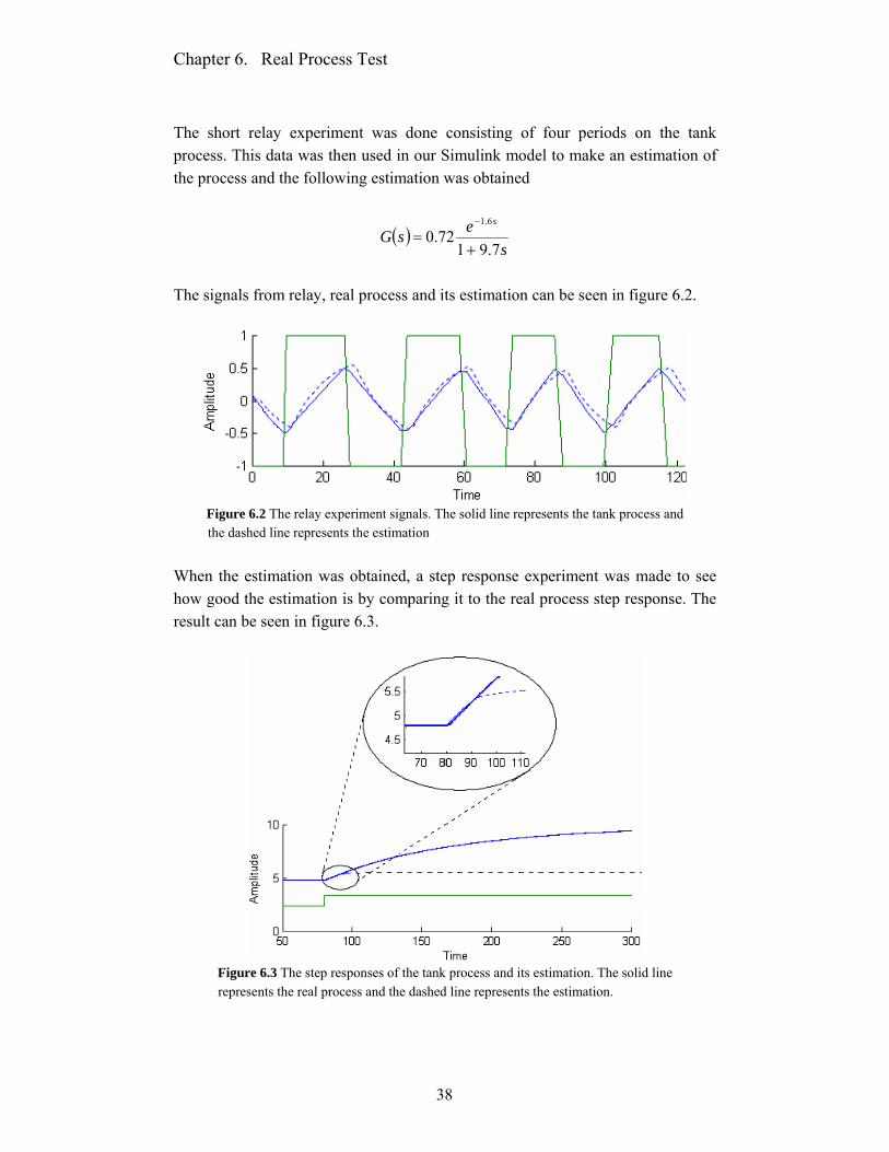
The short relay experiment was done consisting of four periods on the tank process. This data was then used in our Simulink model to make an estimation of the process and the following estimation was obtained
( )s
esGs
7.9172.0
6.1
+=
−
The signals from relay, real process and its estimation can be seen in figure 6.2.
Figure 6.2 The relay experiment signals. The solid line represents the tank process and
the dashed line represents the estimation When the estimation was obtained, a step response experiment was made to see how good the estimation is by comparing it to the real process step response. The result can be seen in figure 6.3.
Figure 6.3 The step responses of the tank process and its estimation. The solid line
represents the real process and the dashed line represents the estimation.

Chapter 6. Real Process Test
39
As it is seen, the same results are obtained as in chapter 4 when ten different processes were estimated. The estimation of the static gain is not correct but the estimation follows the process well at high frequencies.
6.2 Control of a Tank Process To see how good the obtained control is using the AMIGO design, the ECA600 controller was used as a comparison. The ECA600 is a serial PI/PID-controller that uses relay experiment for auto tuning. It is an advanced controller that does not estimate any first order model with time delay of the process to be controlled. Instead, it uses other methods to obtain the controller parameters presented in [7]. When the auto tuning with ECA600 was done, the obtained controller was in PI form. To make a fair comparison, the AMIGO design for PI control, see (2.6), was used to calculate a PI controller parameters. Later, the comparison between the parameters done using a PI controller in Simulink. The values of ECA600 controller and controller using AMIGO are presented in table 6.1.
Process Parameters ECA600 AMIGO Kc 9.46 2.13
Tank process Ti 3.0 7.24
Table 6.1 Controller parameters of ECA600 controller and AMIGO To compare the controllers, a step was applied as reference value to the tank process and, at approximately 200 seconds, a load disturbance was added. The load disturbance was made by opening a valve that can bee seen in figure 6.1 beside the lower tank. The results are shown in figures 6.4 and 6.5.
Figure 6.4 Step response and load disturbance using a controller with ECA600 parameters
Chapter 6. Real Process Test
40
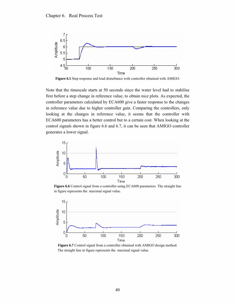
Figure 6.5 Step response and load disturbance with controller obtained with AMIGO.
Note that the timescale starts at 50 seconds since the water level had to stabilise first before a step change in reference value, to obtain nice plots. As expected, the controller parameters calculated by ECA600 give a faster response to the changes in reference value due to higher controller gain. Comparing the controllers, only looking at the changes in reference value, it seems that the controller with ECA600 parameters has a better control but to a certain cost. When looking at the control signals shown in figure 6.6 and 6.7, it can be seen that AMIGO controller generates a lower signal.
Figure 6.6 Control signal from a controller using ECA600 parameters. The straight line
in figure represents the maximal signal value.
Figure 6.7 Control signal from a controller obtained with AMIGO design method.
The straight line in figure represents the maximal signal value.
Chapter 6. Real Process Test
41
6.3 Comment As shown in previous sections, the control obtained with AMIGO design is satisfying. However, there are few comments on the experiment. Since only the control with control parameters in table 6.1 are compared, the reference value change of an ECA600 controller shown in figure 6.4 is not completely correct. In reality, there are filters and other improvements in ECA600 that makes the reference value change smoother. It was noticed that the working point of ECA600 was at higher frequency when the relay experiment was done. If our working point was at even higher frequency, maybe a better estimation could be done. The results are however satisfying even if the process was a very simple one. We believe that the method of estimation presented in this master thesis is more suitable for higher order processes.

42
Chapter 7
Conclusions
7.1 Summary The aim of this thesis was to investigate if it is possible to approximate an unknown process as a first order process with delay only by obtaining information from a relay experiment. If there is a satisfying first order process approximation, there are rules, called AMIGO rules, that gives good PI-/PID controller parameters. By only using the relay experiment, many disadvantages with a step response experiment used in many commercial automatic tuners based on relay feedback, could be avoided. The algorithm used for the optimization of the approximated process parameters is the Gauss-Newton method. To determine the initial values of Kp, T and L for the optimization algorithm, the backward AMIGO design rules are used. The controller parameters Kc, Ti and Td used in backward AMIGO are obtained with modified Ziegler-Nichols update rules. It is difficult to say if it is completely possible to do the approximation well for wide range of processes, but in the tested processes it is shown that 9 of 10 process estimations work well. Although the 10 tested processes are carefully chosen to cover a wide range of process varieties, there have to be done more tests to confirm that.

Chapter 7. Conclusions
43
7.2 Future Work There are a lot of things that could possibly improve the process of finding the initial values and optimizing them. We had a lot of ideas that could work but due to lack of time, i.e. time range of the master thesis, all the ideas could not be evaluated. Some of them and few other, not implemented, ideas are:
• Introduce a method in Gauss-Newton algorithm, called line search, which optimizes the step length in the algorithm where the parameters are updated. This could make the algorithm less sensitive to bad initial values.
• Since a very good estimation of the parameter L can be made, the first order process that approximates the unknown process can be seen as a process with only two unknown parameters, Kp and T. It may be easier to find better estimations of these two parameters if the algorithm optimizes only them instead of all three parameters as it is done in this thesis.

44
Appendix A

45
Appendix B
The relay feedback with real process
The estimation in state space form

46
Appendix C m-file intialvaluegenerator.m for calculation of the initial parameters a=0.05; %relay output b=0.0359; %relay input time=68; %simulation time Tperiod=15.9; %period time of relay input L=3.87; %observed inital L % Calculation of the control parameters K_0=0.35*((pi*b)/(4*a)); Ti=0.40*Tperiod; Td=0.14*Tperiod; % Calculation of the inital parameters using backwards AMIGO const=((2.5*Ti+0.8*Td)/2); L1=const-sqrt(const^2-4.85*Td*Ti); T=(0.3*Td*L1)/(0.5*L1-Td); K=(1/K_0)*(0.2+0.45*T/L1); m-file paramitr.m for iteration of the parameters %Initialization of the process parameters x=[K,T,L]'; %K,T,L calculated in intialvaluegenerator.m %Iteration of the parameters %================================================================== for i=1:8 sim('model1',[0 time]); n1=size(Jx1); n1=n1(1); Jx1=Jx1(n1); n2=size(Jx2); Jx2=Jx2(n2(1)); n3=size(Jx3); Jx3=Jx3(n3(1)); n11=size(Jxx11);

Appendix C
47
Jxx11=Jxx11(n11(1)); n12=size(Jxx12); Jxx12=Jxx12(n12(1)); n13=size(Jxx13); Jxx13=Jxx13(n13(1)); n22=size(Jxx22); Jxx22=Jxx22(n22(1)); n23=size(Jxx23); Jxx23=Jxx23(n23(1)); n33=size(Jxx33); Jxx33=Jxx33(n33(1)); Jx=[Jx1 Jx2 Jx3]'; Jxx=[Jxx11 Jxx12 Jxx13; Jxx12 Jxx22 Jxx23; Jxx13 Jxx23 Jxx33]; x=x-Jxx\Jx; %updating the parameters K=x(1); T=x(2); L=x(3); end SimulationBodNyqStep %plotting of bode, nyquist and stepresponse m-file SimulationBodNyqStep.m for plotting hold off; clf; s=tf('s'); %Initialization of the parameters of the proces to be estimated a=0.5; T0=10; n=8; process=3; %First order model systm=K/(1+s*T); set(systm,'InputDelay',L); %Different tested processes if process==1 systp=K0/(1+s*T0); set(systp,'InputDelay',L0); elseif process==2 systp=1/(1+s*T0)^2;
Appendix C
48
set(systp,'InputDelay',1) elseif process==3 systp=1/((1+s)*(1+s*T0)^2); elseif process==4 systp=1/((1+s)*(1+a*s)*(1+a^2*s)*(1+a^3*s)); elseif process==5 systp=1/(s+1)^n; end %Plot of step response figure(1); t=0:0.1:300; yp=plot(t,step(systm,t)); axis([0 10 -0.005 1.5]); set(yp,'Linewidth',1); xlabel('Time','FontSize',10); ylabel('Amplitude','FontSize',10); hold on t=0:0.1:300; Yp=plot(t,step(systp,t),'-.'); axis([0 10 -0.005 1.5]); set(Yp,'Linewidth',1); set(Yp,'Color','mag'); xlabel('Time','FontSize',10); ylabel('Amplitude','FontSize',10); hold off; %Plot of Nyquist figure(2); [re,im,w]=nyquist(systm,logspace(-3, 4, 10000)); yp=plot(re(:),im(:)); set(yp,'Linewidth',1); hold on axis([-0.1 1 -0.55 0.11]) plot([-2 2.4],[0 0]) plot([0 0],[-3 1.1]) yp=plot(0.15,-0.98,'k<'); set(yp,'Linewidth',1); [mag,phase,w]=bode(systm); hold on; [Re,Im,W]=nyquist(systp,logspace(-3, 4, 10000)); Yp=plot(Re(:),Im(:),'-.'); set(Yp,'Linewidth',1); set(Yp,'Color','mag'); hold on axis([-0.1 1 -0.55 0.11]) plot([-2 2.4],[0 0]) plot([0 0],[-3 1.1]) Yp=plot(0.15,-0.98,'k<'); set(Yp,'Linewidth',1); set(Yp,'Color','mag');

Appendix C
49
[Mag,Phase,W]=bode(systp); hold off; %Plot of Bodediagram figure(3) subplot(2,1,1); yp=loglog(w,mag(:)); set(yp,'Linewidth',1); ylabel('Magnitude','FontSize',10); tmpa=gca; set(tmpa,'Ytick',[0.01 0.1 1]); set(tmpa,'Xtick',[0.1 1 10 100]); axis([0 100 0.1 2]); hold on Yp=loglog(W,Mag(:),'-.'); set(Yp,'Linewidth',1); set(Yp,'Color','mag'); ylabel('Magnitude','FontSize',10); Tmpa=Gca; set(Tmpa,'Ytick',[0.01 0.1 1]); set(Tmpa,'Xtick',[0.1 1 10 100]); axis([0 100 0.1 2]); hold off subplot(2,1,2); yp=semilogx(w,phase(:)); axis([0 100 -200 0]); set(yp,'Linewidth',1); xlabel('Frequency','FontSize',10); ylabel('Phase','FontSize',10); tmpa=gca; set(tmpa,'Xtick',[0.1 1 10 100]); hold on Yp=semilogx(W,Phase(:),'-.'); axis([0 100 -200 0]); set(Yp,'Linewidth',1); set(Yp,'Color','mag'); Tmpa=Gca; set(Tmpa,'Xtick',[0.1 1 10 100]); xlabel('Frequency','FontSize',10); ylabel('Phase','FontSize',10); hold off

50
Bibliography [1] Böiers, L.-C., 2004. Lectures on Optimization, KFS AB, Lund, Sweden. [2] Schmidtbauer, B., 1997. Analog och Digital Reglerteknik, Studentlitteratur,
Lund [3] Slotine, E. J-J., and Weiping, L., 1991. Applied Nonlinear Control, Prentice-
Hall, Inc., Upper Saddle River, New Jersey, USA. [4] Åström, K. J., and Wittenmark, B., 1995. Adaptive Control, 2nd Edition.
Addison-Wesley Publ. Co., Reading, Massachusetts, USA. [5] Åström, K. J., and Hägglund, T., 2005. Advanced PID Control, ISA-The
Instrumentation, Systems and Automation Society, Research Triangle Park, NC 27709, USA.
[6] Åström, K. J., and Hägglund, T., 2004. Revisiting the Ziegler-Nichols step
responce method for PID control, Journal of Process Control, 14, 635-650. [7] Åström, K. J., and Hägglund, T., 1991. Industrial Adaptive Controllers
Based on Frequency Response Techniques, Automatica, Vol. 27, No. 4, 599-609
[8] Åström, K. J., 2004, Introduction to Control, Department of Automatic
Control, Lund Institute of Technology, Lund University, Lund, Sweden.