process exploration by fractional factorial design (ffd)

Process exploration by Fractional Factorial Design (FFD)

Number of Experiments

Factorial design (FD) with variables at 2 levels.

The number of experiments = 2m, m=number of variables.

m=3 : 8 experiments

m=4 : 16 experiments

m=7 : 128 experiments

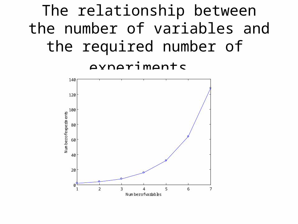
The relationship between the number of variables and the required number of

experiments

1 2 3 4 5 6 70

20

40

60

80

100

120

140

Number of variables

Num

be

r o

f exp

eri

me

nts

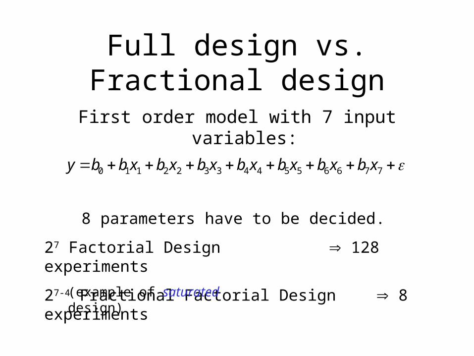
Full design vs. Fractional design

First order model with 7 input variables:

776655443322110 xbxbxbxbxbxbxbby

8 parameters have to be decided.

27 Factorial Design 128 experiments

27-4 Fractional Factorial Design 8 experiments(example of saturated design)

Screening designs

• 27-4 Reduced Factorial Design7 factors in 8 experiments

• 211 Plackett-Burman11 factors in 12 experiments

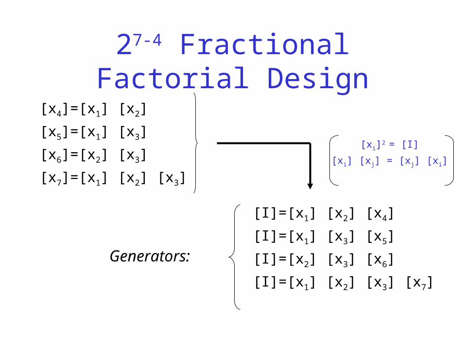
27-4 Fractional Factorial Design

[x4]=[x1] [x2]

[x5]=[x1] [x3]

[x6]=[x2] [x3]

[x7]=[x1] [x2] [x3]

[I]=[x1] [x2] [x4]

[I]=[x1] [x3] [x5]

[I]=[x2] [x3] [x6]

[I]=[x1] [x2] [x3] [x7]

[xi]2 = [I]

[xi] [xj] = [xj] [xi]

Generators:

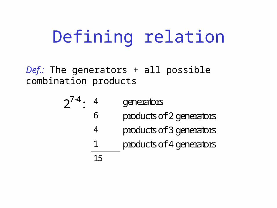
Defining relation

Def.: The generators + all possible combination products

27-4: 4 generators

6 products of 2 generators



15

Defining relation for 27-4 FFD

[I] = [x1] [x2] [x4] = [x1] [x3] [x5] = [x2] [x3] [x6] = [x1] [x2] [x3] [x7] = [x2] [x4] [x3] [x5] = [x1] [x4] [x3] [x6]= [x4] [x3] [x7] = [x1] [x2] [x5] [x6] = [x2] [x5] [x7]= [x1] [x6] [x7] = [x4] [x5] [x6] = [x2] [x4] [x6] [x7]= [x1] [x4] [x5] [x7] = [x3] [x5] [x6] [x7] = [x1] [x2] [x3] [x4] [x5] [x6] [x7]

The confounding pattern appears by multiplying the defining relation with each of the variables.

Process capacity

Box and Hunter, 1961, Technometrics 3, p. 311

Variable -1 +1

X1 Water Source City reservoir Private well

X2 Raw material Local Other

X3 Temperature Low High

X4 Recycling Yes No

X5 Caustic Soda Fast Slow

X6 Filter New Old

X7 Waiting time Short Long

The Design Matrix

Response Variation

Estimates of the effects

Effect Estimate

1 X1+ X2X4 + X3 X5+ X6 X7 -5.4 2 X2 + X1X4 + X3 X6+ X5 X7 -1.4 3 X3 + X1X5 + X2 X6+ X4 X7 -8.3 4 X4 + X1X2 + X3 X7+ X5 X6 1.6 5 X5 + X1X3 + X2 X7+ X4 X6 -11.4 6 X6 + X1X7 + X2 X3+ X4 X5 -1.7 7 X7 + X1X6 + X2 X5+ X3 X4 0.26

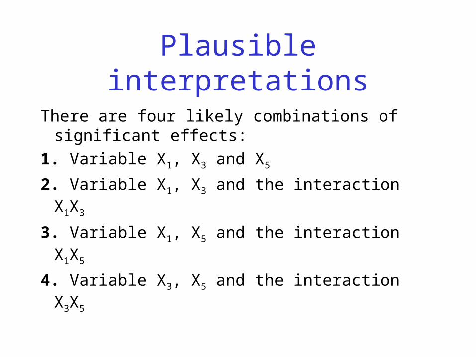
Plausible interpretations

There are four likely combinations of significant effects:

1. Variable X1, X3 and X5

2. Variable X1, X3 and the interaction X1X3



New experimental series

It is desirable to separate the 1- and 2- factor effects.

[x4]= - [x1] [x2]

[x5]= - [x1] [x3]

[x6]= - [x2] [x3]

[x7]= - [x1] [x2] [x3]

A new 27-4-design with a different set of generators is generated:

The Design Matrix-new experimental series

Estimates of the effects

Effect Estimate

1 X1- X2X4 - X3 X5- X6 X7 -1.32 X2 - X1X4 - X3 X6- X5 X7 -2.5 3 X3 - X1X5 - X2 X6- X4 X7 7.9 4 X4 - X1X2 - X3 X7- X5 X6 1.1 5 X5 - X1X3 - X2 X7- X4 X6 -7.8 6 X6 - X1X7 - X2 X3- X4 X5 1.77 X7 - X1X6 - X2 X5- X3 X4 -4.6

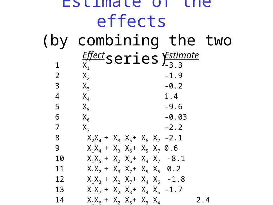
Estimate of the effects (by combining the two series)

Effect Estimate1 X1 -3.32 X2 -1.9 3 X3 -0.24 X4 1.4 5 X5 -9.6 6 X6 -0.037 X7 -2.2 8 X2X4 + X3 X5+ X6 X7 -2.19 X1X4 + X3 X6+ X5 X7 0.610 X1X5 + X2 X6+ X4 X7 -8.111 X1X2 + X3 X7+ X5 X6 0.212 X1X3 + X2 X7+ X4 X6 -1.813 X1X7 + X2 X3+ X4 X5 -1.714 X1X6 + X2 X5+ X3 X4 2.4

Contour plot

Filter time, y (min)

Interpretation

Water source

65.4 42.6

68.5 78.0

Caustic Soda

Slow

FastCity

ReservoirPrivate

Well

i) Slow addition of NaOH improves the response (shorten the filtration time)

ii) The composition of the water in the private wells (pH, minerals etc.) is better than the water from the city reservoir with respect to the response (tends to shorten the filtration time)

Bottom line...

Univariate optimisation of the speed used for adding NaOH!

This result would not have been obtained by a univariate approach!

process exploration by fractional factorial design (ffd)

Documents