process optimization via simulated annealing:...

Process Optimization via Simulated Annealing: Application to Network Design

Simulated annealing is a multivariable optimization technique based on the Monte Carlo method used in statistical mechanical studies of condensed systems and follows by drawing an analogy between energy minimization in physical systems and costs minimization in design applications. In this paper, simulated annealing is introduced and reviewed. The utility of the method for optimization of chemical processes is illustrated by applying it to the design of pressure relief header networks and heat exchanger networks.

Introduction Computer-aided chemical process design and optimization in-

creasingly play an important role in reducing the time lag between process innovation and commercial implementation, in ensuring the efficiency and flexibility of new chemical plants, and in improving the operating efficiencies of existing plants.

This paper applies the simulated annealing algorithm to design problems in chemical engineering. Simulated annealing is a general method for treating a broad class of large, multivariable optimization problems. It has found wide application in the physical sciences and engineering, but evidently not previously to problems in chemical engineering.

The simulated annealing algorithm was proposed by Kirkpa- trick et al. (1 983), who drew an analogy between the cooling of a fluid and the optimization of a complex system. In order for a pure substance to be ‘frozen’ into a perfect or nearly perfect crystal, it must be annealed by first melting and then cooling very slowly. If the substance is cooled too quickly, a crystal with many defects or a glass will be formed; the resulting structure will be far from the highly ordered, minimum energy, crystalline state. To illustrate the effectiveness of simulated annealing, Kirkpatrick et al. (1983) applied the method to two combinatorially large optimization problems: the traveling salesman problem and the layout of very-large-scale integrated (VLSI) circuit computer chips. For the latter, the placement and wiring of several thousand discrete circuit elements are principal concerns. In general, the shorter the connections are between the elements, the more optimal is the design; however, the circuit elements cannot be placed too close together since they can inter- fere with each other. Simulated annealing has now become a standard technique for designing VLSI chips. In particular, it is often used to assess whether designs obtained by other, perhaps heuristic, methods can be improved upon by starting the anneal-

W. B. Dolan P. T. Cummings

M. D. LeVan Department of Chemical Engineering

University of Virginia Charlottesville, VA 22901

ing a t relatively low temperature using the proposed design as the initial configuration.

Simulated annealing is based on the theory of Markov chains, as described below. It accepts and rejects randomly generated ‘moves’ on the basis of a probability related to an ‘annealing temperature’. It can accept moves which change the value of an objective function in the direction opposite to that of the desired long-term trend. Thus, for a global minimization problem, a move that increases the value of the objective function (an ‘uphill’ move) may be accepted as part of the full series of moves for which the general trend is to decrease the value of the objective function. In this way, simulated annealing is able to explore the full solution space and solutions are independent of the starting point. This means that one does not become trapped in a far from optimal local minimum as is possible with algorithms based on Newton’s method.

Simulated annealing has proven to be a practical method for solving combinatorially large optimization problems. Press et al. (1986) report that simulated annealing can obtain solutions to combinatorial optimization problems within specified ‘dis- tances’ of the global optimum in computational time that is pro- portional to N”, where N is a measure of the size of the problem and n is a small positive number. For example, Aarts and van Laarhoven (1985) report a simulated annealing method for the N-city traveling salesman problem that yields solutions within 2% of the global optimum and grows as N3. Algorithms which are guaranteed to find the global optimum for such problems increase in computational time much more quickly and, in the worst case, are exponential in N.

With simulated annealing, the minimization of a global objective function is approached directly. When applied to a problem of cost minimization, moves are accepted and rejected based on a cost function. No heuristic arguments are needed.

AIChE Journal May 1989 Vol. 35, No. 5 725

Instead, both capital costs and operating expenses are contained in the cost function and its global minimum is sought. If, for some reason, constraints are to be built into the problem, this can be easily done. Any move which would violate a constraint can be rejected outright or penalized through the cost function.

One of the great strengths of simulated annealing is the ease with which discrete variables and discontinuous cost functions can be handled. Off-the-shelf supplies and equipment are often available in standard sizes and capacities. Construction costs can be reduced significantly if special fabrication is not required. For example, the cost of a standard heat exchanger is roughly 50 to 75% of that for a custom-built exchanger (Rubin et al., 1984). Similarly, pipes are readily available only in standard sizes. Thus, with simulated annealing, in contrast to many popular algorithms, it is not necessary to solve a problem in terms of continuous variables, only later to have to replace them with standard sizes.

As explained below in detail, we have adopted terminology of statistical mechanics to classify problems into two types: 'canonical' problems, for which the number of elements is fixed, and 'grand canonical' problems, for which the number of elements in the problem varies as the solution is obtained. To our knowledge, problems treated previously using simulated annealing have all been of the canonical type. Thus, our consideration of grand canonical problems is a contribution to the development of simulated annealing as a general methodology for multivariable optimization.

Two types of problems are considered in this paper: the design of a pressure relief header network (a canonical problem) and the design of a heat exchanger network (a grand canonical problem).

Theory Simulated annealing is based on the Monte Carlo simulation

technique developed by Metropolis et al. (1 953) to study the statistical mechanics of condensed systems (dense gases, liquids, and solids). More precisely, the Metropolis algorithm permits the direct simulation of the so-called canonical ensemble of statistical mechanics, in which the number of molecules N, the volume V, and the temperature T of the system are held fixed. In so doing, it asymptotically generates low-energy configurations of the system at fixed N , V, and T. The variables that can be manipulated to generate these low-energy configurations are the positions and orientations of the molecules.

In this section, the Metropolis algorithm for the simulation of condensed physical systems is reviewed. In addition, the algorithm for simulating the so-called grand canonical ensemble of statistical mechanics (in which V, T and the chemical potential pi of each species are held fixed and N is not prescribed but rather is determined in the course of the simulation) is described. Finally, the simulated annealing algorithm is present ed .

Monte Carlo simulation of condensed systems The mathematics underlying the Metropolis algorithm are

given elsewhere (Hammersley and Handscomb, 1964; Valleau and Whittington, 1977) and are beyond the scope of this paper. For simplicity, the Metropolis algorithm will be described for a pure fluid composed of spherically symmetric molecules.

In Monte Carlo simulations of condensed systems, the config- urational energy E, which the molecules possess by virtue of their positions and which is calculated from the intermolecular potentials, is determined. E is given completely by the set of (7.1, i = I , . . .. N wherez, is the position of molecule i in the system. Equivalently, one can define the configuration state + of a system of N molecules by the phase vector?" = (?,,T2, . . ., rN), a vector in 3N-$mensional phase space. The energy E is clearly a function of rN,

E = E (?")

The object of the Metropolis algorithm is to generate a series of points in phase space which are distributed according to the canonical ensemble Boltzmann probability density

P(?") a exp ( - E ( F N ) / k B T )

where kB is Boltzmann's constant. The Metropolis algorithm is a rigorously correct formalism

for generating a Markov chain (Karlin, 1973) of points in phase space that asymptotically are distributed according to Eq. 2 and are independent of the initial point. The algorithm for generating a sequence of points in phase space is given by the following steps:

(i) Initialize the positions of the molecules (i.e., initialize

(ii) Choose a molecule a t random and move it randomly to a new position (randomly generate in the vicinity of Y N * O f d ) .

(iii) Consider AE = E(?",") - E(?".Ofd) . If A E < 0 (i.e., the energy goes down), then accept the new configuration ?"',nrw.

Otherwise, accept it with probability

P) .

exp ( - A E / k , T ) (3)

(iv) Repeat steps (ii) and (iii) many times while calculating averages of desired properties.

In some circumstances, the Metropolis algorithm does not represent the best method for simulating the physical system of interest. For example, in the simulation of some nonuniform systems, such as the solvent fluid contained between two very large colloidal particles, the appropriate ensemble in which to simu- late the system is the so-called grand canonical ensemble (Ad- ams, 1975; Snook and van Megen, 1981), in which the volume V, temperature T, and chemical potentials pi are fixed, and the numbers of molecules, Ni of species i, fluctuate and come to equilibrium during thezourse of the simulation. In this case, the vector in phase space, r, is of variable length depending on the number of molecules in the simulation a t any given point; it also depends on the species present in the case of a mixture. The algorithm employed in simulation is:

(i) Initialize the positions and number of the molecules (i.e., initialize ?).

(ii) Choose a molecule a t random and move it randomly to a new position.

(iii) Add/delete a molecule of species i. [Steps (ii) and (iii) randomly generateF" in the vicinity of ? O f d . ]

726 May 1989 Vol. 35, No. 5 AIChE Journal

(iv) AcceptS" if E decreases; otherwise, accept it with probability

exp ( - A E / k , T ) (4) for a move of type (ii). For moves involving addition or deletion of a species i molecule, the acceptance criterion depends on AE and the chemical potential of species i molecules (Adams, 1975).

(v) Repeat steps (ii) to (iv) many times. This section is concluded with several observations about both

the canonical ensemble and grand canonical ensemble Monte Carlo algorithms:

1. Asymptotically, the configurations generated will be low- energy configurations due to the nature of the probability distribution governing the ensembles.

2. The algorithms have the capability of 'climbing out' of local minima in the energy function since uphill moves are per- missible.

3. The proportion of uphill moves accepted increases with temperature.

Physically, one type of local energy minimum that can arise is the amorphous glassy state which is obtained by a rapid temperature drop (quench) from a disordered fluid state. In fact, one can easily generate glassy state configurations using simulation by starting with a disordered liquid and rapidly quenching it. The likelihood of making a transition out of the quenched glassy state is extremely low, since to reach the lowest energy, ordered crystalline state an energy barrier must be overcome but the probability of making the necessary uphill moves is very low when the system temperature is low. Thus, in order to generate a lowest energy, crystalline state from an initially fluid system, one must lower the temperature very gradually, allowing the system to approach equilibrium at each temperature. This process of annealing, as opposed to quenching, is used to produce nonamorphous crystalline metals in real systems and provides the mechanism in a simulation for bringing a system into the lowest possible energy state.

Simulated annealing Multivariable optimization is the general term used to

describe the process of identifying the set of variables 2 = ( x ] , x2, . . ., x,) which globally minimize an objective function C ( 2 ) (which, without loss of generality, can be regarded as the cost associated with the particular choice of 2). Kirkpatrick et al. (1 983) conjectured that multivariable optimization problems involving a large number of variables might be solved efficiently using a generalization of the canonical ensemble Monte Carlo algorithm. An analogy was drawn between energy in canonical ensemble physical systems and cost in multivariable optimization and between the phase point ?" and the vector 5;. Since, as noted above, if a physical system is annealed to extremely low temperature, it will eventually find itself in the lowest energy configuration, Kirkpatrick and coworkers suggested that by per- forming an analogous 'annealing' procedure on a multivariable optimization problem the vector 5; which globally minimized C ( 2 ) would be located.

This identification requires that within the optimization context an analog of the temperature of physical systems must be identified. Kirkpatrick et al. introduced the concept of a simulated annealing temperature, T,, which has the units of cost and is used to control the probability for accepting uphill moves in

cost. The simulated annealing temperature starts out at a high value so that a high proportion of attempted changes in 2 are accepted. As the simulation progresses, T, is reduced periodically, according to a prescription known as the nnneahg schedule. With each reduction in T,, the proportion of accepted moves goes down until, eventually, no moves are accepted. This implies that all attempted moves are uphill in cost and that the temperature is low enough that these moves are no longer accepted. Provided the annealing has been performed slowly enough, the final 2 should represent the global minimum of

The simulated annealing algorithm of Kirkpatrick et al.

(i) Initialize 7 and T,. (ii) Choose an element of? at random and change it ran-

domly to a new value (i.e., randomly generatex- in the vicinity

(iii) Consider AC = C(?'") - C(?'ld). If AC < 0 (i.e., the cost decreases), then accepted the new vector 2-. Otherwise, accept it with probability.

C(2).

(1 983) is given by:

of Pd).

(5)

(iv) Repeat steps (ii) and (iii) many times while periodically reducing T,. The annealing schedule of Kirkpatrick et al. involved reducing the annealing temperature according to

where 5 is a constant somewhat less than unity and n represents the nth annealing temperature. Notice that this algorithm is very similar to the canonical ensemble Metropolis algorithm for physical systems described above. The common feature that this algorithm and the canonical algorithm share, which differs from the grand canonical algorithm, is that the number of variables manipulated in each case is fixed; i.e.,FN and 2 have a constant number of elements. With this in mind, it is appropriate to cate- gorize the simulated algorithm presented here as being appropriate for 'canonical' optimization problems.

As developed in this paper, there is a natural generalization of the grand canonical ensemble Monte Carlo simulation algorithm that would be applicable to 'grand canonical' optimization problems in which the number of variables to be manipulated is not fixed and is unknown before the optimization is performed.

In statistical mechanics, the critical element in the utility of Monte Carlo simulation is that the asymptotic distribution of points in phase space is independent of the starting configuration. This is proved using the mathematical theory of Markov chains (Hammersley and Handscomb, 1964) and suggests that in the optimization context, simulated annealing is capable of producing the global optimum independent of the initial guess. Several formal proofs have been given which establish that, if the number of attempted moves at each temperature is infinite, simulated annealing produces asymptotically the global optimum solution of combinatorial optimization problems with probability one (Romeo and Sangiovanni-Vincentelli, 1984; Lundy and Mees, 1984). In practice, one cannot guarantee that the solution obtained by simulated annealing in a finite amount of time is the rigorous optimum; however, the formal results suggest that a sufficiently slow annealing schedule will provide an optimal or near-optimal solution that is independent of the initial guess and therefore, in principle, avoids becoming trapped in


local minima of the cost function that lie between the initial guess and the global optimum.

The random nature of the move used in a simulated annealing algorithm to create a new design might suggest that the method is similar to the adaptive random search algorithms described by Martin and Gaddy (1982). In the latter algorithms, to generate xnCW and ;Old, many points; in the vicinity of ?‘Id are generated randomly and the one with the lowest cost becomes Tmw. Thus, only downhill moves in cost are considered and the adaptive random search methods are therefore very likely to become trapped in a local minimum of the cost function. Consequently, the only similarity between simulated annealing and the adaptive random search method is that new designs are generated stochasti- cally.

+

‘Canonical’ Optimization: Pipeline Networks The general problem of optimal design of fluid transportation

systems is common throughout the chemical processing indus- try. In many cases the objective is to minimize the transportation cost subject to regulatory and opertting constraints. Nor- mally, the layout of the transportation network is fixed, and the problem that remains to be solved is balancing pressure drop requirements against pumping cost or throughput.

Simulated annealing has been applied to two examples of fluid transportation network optimization: the design of a pressure relief header network (described in this section) and the design of a compressible fluid network (Wohlpart. 1987). Both problems are ‘canonical’ optimization problems since, in each case, the objective function (cost) is minimized with respect to a fixed number of variables (pipe diameters in the case of the pressure relief header network, pipe diameters and compressor duties in the case of the compressible fluid transport problem). The success of simulated annealing on these two problems serves to confirm that, with very little effort required on the part of the user, the algorithm is capable of obtaining a near minimum cost solution to canonical optimization problems that arise in chemical process design.

In the remainder of this section, the application of simulated annealing to pressure relief header network design will be described in detail. The role of a pressure relief header network in a chemical plant is to transport fluids as expediently as possible from process equipment to the flare head. This requires that sonic velocity be maintained in the discharge valves connecting the process equipment to the flare for an initial transitory peri- od. Maintaining sonic velocity through a valve requires that the pressure on the downstream side of the valve remain below a certain value, which is determined by process conditions and the valve. This pressure sets a maximum allowable pressure drop between the valve and the flare. For a network, maximum allowable pressure drops are specified between downstream sides of valves and the flare, creating a set of constraints on the design.

We consider the problem of Cheng (1976), the qualitative features of which have been discussed by Cheng and Mah ( 1976). The problem has also been considered by Murtagh (1 972). who describes a method that will give the optimum solution based on a continuous set of pipe diameters. Cheng solved the problem by the discrete merge method, which has its foun- dation in dynamic programming and is suitable for certain fixed structures. It can accommodate discrete pipe sizes and generates lists of pipe sections by serial and parallel merging.

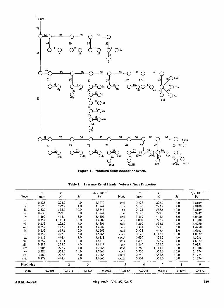
Although Cheng and Mah (1976) describe the discrete merge method as applied to the pressure relief header network problem, neither the full problem description nor a solution is contained in their paper; Cheng ( 1 976) gives the problem description, his computer program, and a solution. Figure 1 depicts the pressure relief network. The full problem description is given in Tables 1 and 2. As shown in Figure 1 , there are 79 pipe segments and 34 source nodes. For each pipe segment there are nine possible choices, given a t the bottom of Table 1, for the pipe segment diameter. It should be clear that the number of different combinations of pipe diameters is extremely large for this problem; in fact, with nine different pipe diameters possible for each segment, the number of possible designs is 979. Thus, any solution method employed must be selective of the solution space it searches.

The pressures a t the upstream ( A ) and downstream ( B ) end of a pipe segment for compressible flow are related by

0.36!9!9h752XT [ 1 + - 4.61 d 4f 1

P: - P e = (7)

where

I = II, + II,, I n this equation, P, is the straight length and II, is the additional equivalent length. Following Cheng and Mah, the group in brackets in Eq. 7 (a kinetic energy correction term) is close t o unity giving

In calculating temperatures of streams formed by mixing, the mixing rule used is simply

i I i (9)

where W, is the mass flowrate of stream i. The cost of the network is determined by the capital cost of

the pipe segments. The cost of a pipe is assumed to be a linear function of its diameter. Thus, the cost of a pipe of diameter d is simply

c = (a + Bd) Ps

where a and p are constants. From Eq. 10, it is clear that the cost function in this optimization problem is linear in the variables 2 = ( d l , d2, . . . , d N ) where N is the number of pipe segments in the network. The nonlinearity in this problem arises through the pressure constraints which can be written as

where S, is the set of pipes between node i and the flare. Values of bi are listed in Table 1.

We developed our own computer program implementing the discrete merge method described by Rothfarb et al. (1970) and


lnarej I

38 n 36 Y

p V l i i

ix

55 xi

6% xv

K7Z xvi xvii

XIV

xxviii xxxi xxvi

Figure 1. Pressure relief header network.

Table 1. Pressure Relief Header Network Node Properties

W T bi x F T b, x lo-'* Node kg/s K M Pa' Node kg/s K M Pa2

I 0.126 222.2 4.0 I I 2.520 222.2 4.0

i i i 2.520 555.6 10.0 iv 0.630 277.8 5.0 V 1.260 444.4 8.0

vi 0.252 1,111.1 10.0 vii 0.252 222.2 4.0

0.252 222.2 4.0 ix 0.252 555.6 10.0 X 0.252 277.8 5.0

xi 0.126 444.4 8.0 xii 0.252 1,111.1 10.0

xiii 0.882 222.2 4.0 xiv 1.008 222.2 4.0 xv 3.780 555.6 10.0

xvi 3.780 277.8 5.0 xvii 0.378 444.4 8.0

... Vl l l

3.3277 3.3844 3.3844 3.3844 3.4507 3.4507 3.4507 3.4507 3.5265 3.5265 3.6118 3.61 18 3.61 18 3.7066 3.7066 3.7066 3.1066

xviii xix

xxi xxii

xxiii xxiv

xxvi xxvii

xxviii xxix

xxxi xxxii

xxxiii xxxiv

xx

xxv

xxx

0.378 222.2 4.0 0.126 222.2 4.0 0.126 555.6 10.0 0.126 271.8 5.0 1.260 444.4 8.0 1.008 222.2 4.0 1.260 555.6 10.0 0.378 277.8 5.0 0.378 444.4 8.0 0.126 1,111.1 10.0 0.630 222.2 4.0 1.890 222.2 4.0 1.260 222.2 4.0 1.260 1,111.1 10.0 0.756 555.6 10.0 0.252 555.6 10.0 0.504 555.6 10.0

3.8109 3.8109 3.8109 3.9247 4.0480 4.1808 4.4750 4.4750 4.6363 4.8072 4.3231 4.8072 5.0351 4.1808 5.1774 5.1774 5.1774

Pipe Index 1 2 3 4 5 6 7 8 9

d, m 0.0508 0.1016 0.1524 0.2032 0.2540 0.3048 0.3556 0.4064 0.4572

AlChE Journal May 1989 Vol. 35, No. 5 729

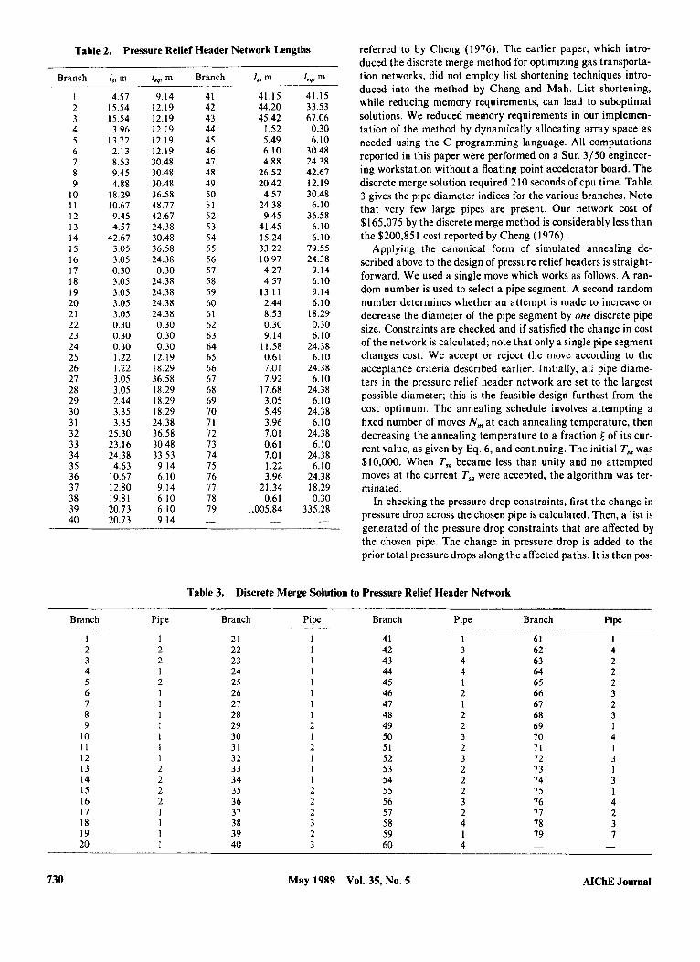
Table 2. Pressure Relief Header Network Lengths

Branch I,, m I,, m

1 2 3 4 5 6 7 8 9

10 11 12 13 14 I5 16 17 18 19 20 21 22 23 24 25 26 27 28 29 30 31 32 33 34 35 36 37 38 39 40

4.57 15.54 15.54 3.96

13.72 2.13 8.53 9.45 4.88

18.29 10.67 9.45 4.57

42.67 3.05 3.05 0.30 3.05 3.05 3.05 3.05 0.30 0.30 0.30 I .22 1.22 3.05 3.05 2.44 3.35 3.35

25.30 23.16 24.38 14.63 10.67 12.80 19.81 20.73 20.73

9.14 12.19 12.19 12.19 12.19 12.19 30.48 30.48 30.48 36.58 48.77 42.67 24.38 30.48 36.58 24.38 0.30

24.38 24.38 24.38 24.38 0.30 0.30 0.30

12.19 18.29 36.58 18.29 18.29 18.29 24.38 36.58 30.48 33.53 9.14 6.10 9.14 6.10 6.10 9.14

41 41.15 42 44.20 43 45.42 44 I .52 45 5.49 46 6.10 47 4.88 48 26.52 49 20.42 50 4.57 51 24.38 52 9.45 53 41.45 54 15.24 55 33.22 56 10.97 57 4.27 58 4.57 59 13.11 60 2.44 61 8.53 62 0.30 63 9.14 64 11.58 65 0.61 66 7.01 67 7.92 68 17.68 69 3.05 70 5.49 71 3.96 72 7.01 73 0.61 74 7.01 75 1.22 76 3.96 77 21.34 78 0.61 79 1,005.84 - -

41.15 33.53 67.06

0.30 6.10

30.48 24.38 42.67 12.19 30.48

6.10 36.58

6.10 6.10

79.55 24.38

9.14 6.10 9.14 6.10

18.29 0.30 6.10

24.38 6.10

24.38 6.10

24.38 6.10

24.38 6.10

24.38 6.10

24.38 6.10

24.38 18.29 0.30

335.28 -

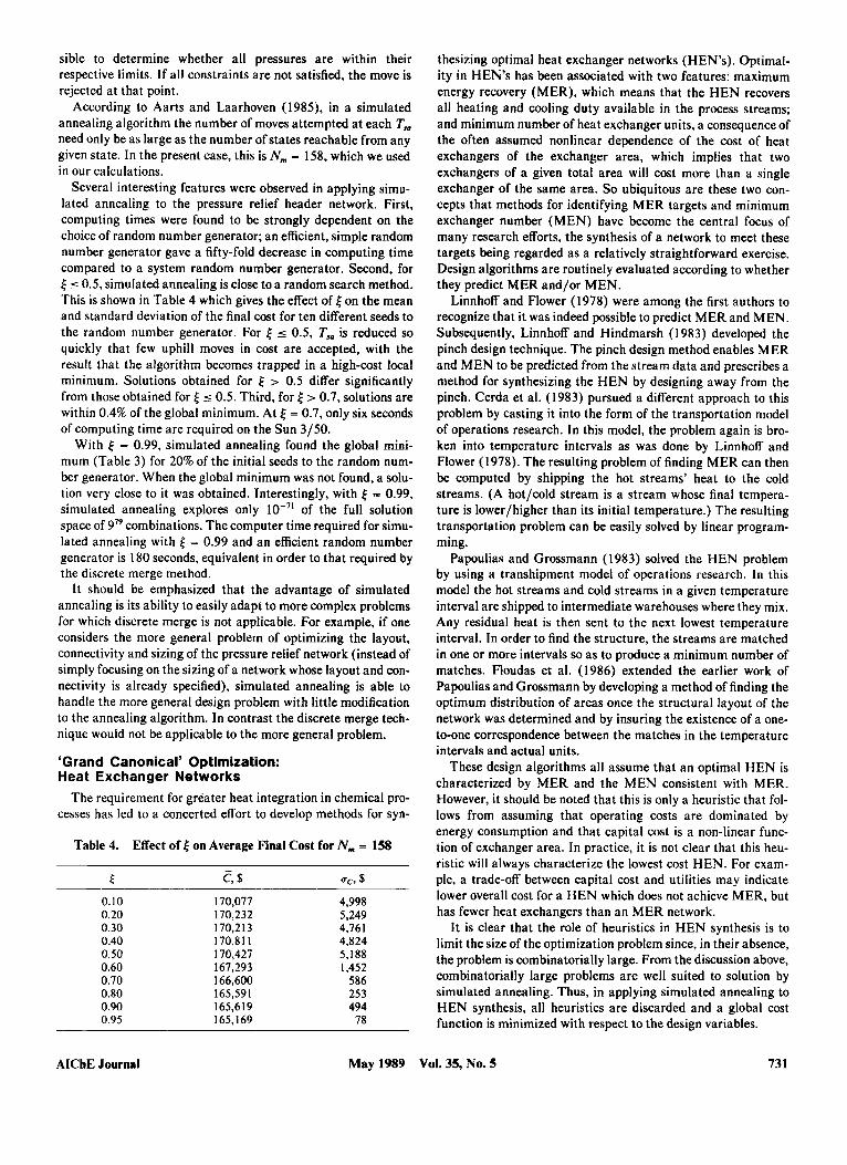
referred to by Cheng (1976). The earlier paper, which introduced the discrete merge method for optimizing gas transportation networks, did not employ list shortening techniques introduced into the method by Cheng and Mah. List shortening, while reducing memory requirements, can lead to suboptimal solutions. We reduced memory requirements in our implementation of the method by dynamically allocating array space as needed using the C programming language. All computations reported in this paper were performed on a Sun 3/50 engineering workstation without a floating point accelerator board. The discrete merge solution required 210 seconds of cpu time. Table 3 gives the pipe diameter indices for the various branches. Note that very few large pipes are present. Our network cost of $165,075 by the discrete merge method is considerably less than the $200,85 1 cost reported by Cheng ( 1 976).

Applying the canonical form of simulated annealing described above to the design of pressure relief headers is straightforward. We used a single move which works as follows. A random number is used to select a pipe segment. A second random number determines whether an attempt is made to increase or decrease the diameter of the pipe segment by one discrete pipe size. Constraints are checked and if satisfied the change in cost of the network is calculated; note that only a single pipe segment changes cost. We accept or reject the move according to the acceptance criteria described earlier. Initially, all pipe diameters in the pressure relief header network are set to the largest possible diameter; this is the feasible design furthest from the cost optimum. The annealing schedule involves attempting a fixed number of moves N,,, a t each annealing temperature, then decreasing the annealing temperature to a fraction E of its current value, as given by Eq. 6, and continuing. The initial T, was $10,000. When T, became less than unity and no attempted moves at the current T, were accepted, the algorithm was terminated.

In checking the pressure drop constraints, first the change in pressure drop across the chosen pipe is calculated. Then, a list is generated of the pressure drop constraints that are affected by the chosen pipe. The change in pressure drop is added to the prior total pressure drops along the affected paths. It is then pos-

Table 3. Discrete Merge Solution to Pressure Relief Header Network

Branch Pipe Branch Pipe Branch Pipe Branch Pipe

I 1 21 1 41 1 61 1 2 2 22 1 42 3 62 4 3 2 23 1 43 4 63 2 4 1 24 1 44 4 64 2 5 2 25 1 45 1 65 2 6 1 26 1 46 2 66 3 7 I 27 1 47 1 61 2 8 1 28 1 48 2 68 3 9 1 29 2 49 2 69 1

10 1 30 I 50 3 70 4 I I I 31 2 51 2 71 1 12 1 32 1 52 3 72 3 13 2 33 1 53 2 73 1 14 2 34 1 54 2 74 3 15 2 35 2 55 2 75 1 16 2 36 2 56 3 76 4 17 1 37 2 57 2 77 2 18 1 38 3 58 4 78 3 19 1 39 2 59 1 79 7 20 I 40 3 60 4 - -


sible to determine whether all pressures are within their respective limits. If all constraints are not satisfied, the move is rejected at that point.

According to Aarts and Laarhoven (1985), in a simulated annealing algorithm the number of moves attempted at each T,a need only be as large as the number of states reachable from any given state. In the present case, this is N,,, = 158, which we used in our calculations.

Several interesting features were observed in applying simulated annealing to the pressure relief header network. First, computing times were found to be strongly dependent on the choice of random number generator; an efficient, simple random number generator gave a fifty-fold decrease in computing time compared to a system random number generator. Second, for 5 5 0.5, simulated annealing is close to a random search method. This is shown in Table 4 which gives the effect of 5 on the mean and standard deviation of the final cost for ten different seeds to the random number generator. For 5 5 0.5, T, is reduced so quickly that few uphill moves in cost are accepted, with the result that the algorithm becomes trapped in a high-cost local minimum. Solutions obtained for > 0.5 differ significantly from those obtained for 5 c 0.5. Third, for 5 > 0.7, solutions are within 0.4% of the global minimum. At 5 = 0.7, only six seconds of computing time are required on the Sun 3/50.

With 5 = 0.99, simulated annealing found the global minimum (Table 3) for 20% of the initial seeds to the random number generator. When the global minimum was not found, a solution very close to it was obtained. Interestingly, with 5 = 0.99, simulated annealing explores only of the full solution space of 979 combinations. The computer time required for simulated annealing with ( = 0.99 and an efficient random number generator is 180 seconds, equivalent in order to that required by the discrete merge method.

It should be emphasized that the advantage of simulated annealing is its ability to easily adapt to more complex problems for which discrete merge is not applicable. For example, if one considers the more general problem of optimizing the layout, connectivity and sizing of the pressure relief network (instead of simply focusing on the sizing of a network whose layout and connectivity is already specified), simulated annealing is able to handle the more general design problem with little modification to the annealing algorithm. In contrast the discrete merge technique would not be applicable to the more general problem.

‘Grand Canonical’ Optimization: Heat Exchanger Networks

The requirement for greater heat integration in chemical processes has led to a concerted effort to develop methods for syn-

Table 4. Effect of 6 on Average Final Cost for N, = 158

0.10 0.20 0.30 0.40 0.50 0.60 0.70 0.80 0.90 0.95

170,077 170,232 170.21 3 170.81 1 170,427 167,293 166,600 165,591 165.6 19 165,169

4,998 5,249 4,161 4,824 5,188 1,452

586 253 494 78

thesizing optimal heat exchanger networks (HEN’s). Optimal- ity in HEN’s has been associated with two features: maximum energy recovery (MER), which means that the HEN recovers all heating and cooling duty available in the process streams; and minimum number of heat exchanger units, a consequence of the often assumed nonlinear dependence of the cost of heat exchangers of the exchanger area, which implies that two exchangers of a given total area will cost more than a single exchanger of the same area. So ubiquitous are these two con- cepts that methods for identifying MER targets and minimum exchanger number (MEN) have become the central focus of many research efforts, the synthesis of a network to meet these targets being regarded as a relatively straightforward exercise. Design algorithms are routinely evaluated according to whether they predict MER and/or MEN.

Linnhoff and Flower (1978) were among the first authors to recognize that it was indeed possible to predict MER and MEN. Subsequently, Linnhoff and Hindmarsh (1983) developed the pinch design technique. The pinch design method enables MER and MEN to be predicted from the stream data and prescribes a method for synthesizing the HEN by designing away from the pinch. Cerda et al. (1983) pursued a different approach to this problem by casting it into the form of the transportation model of operations research. In this model, the problem again is bro- ken into temperature intervals as was done by Linnhoff and Flower (1978). The resulting problem of finding MER can then be computed by shipping the hot streams’ heat to the cold streams. (A hot/cold stream is a stream whose final temperature is lower/higher than its initial temperature.) The resulting transportation problem can be easily solved by linear programming.

Papoulias and Grossmann (1983) solved the HEN problem by using a transhipment model of operations research. In this model the hot streams and cold streams in a given temperature interval are shipped to intermediate warehouses where they mix. Any residual heat is then sent to the next lowest temperature interval. In order to find the structure, the streams are matched in one or more intervals so as to produce a minimum number of matches. Floudas et al. (1986) extended the earlier work of Papoulias and Grossmann by developing a method of finding the optimum distribution of areas once the structural layout of the network was determined and by insuring the existence of a one- to-one correspondence between the matches in the temperature intervals and actual units.

These design algorithms all assume that an optimal HEN is characterized by MER and the MEN consistent with MER. However, it should be noted that this is only a heuristic that follows from assuming that operating costs are dominated by energy consumption and that capital cost is a non-linear function of exchanger area. In practice, it is not clear that this heuristic will always characterize the lowest cost HEN. For example, a trade-off between capital cost and utilities may indicate lower overall cost for a HEN which does not achieve MER, but has fewer heat exchangers than an MER network.

It is clear that the role of heuristics in HEN synthesis is to limit the size of the optimization problem since, in their absence, the problem is combinatorially large. From the discussion above, combinatorially large problems are well suited to solution by simulated annealing. Thus, in applying simulated annealing to HEN synthesis, all heuristics are discarded and a global cost function is minimized with respect to the design variables.


The simulated annealing algorithm required for HEN synthesis is based on analogy with the Metropolis algorithm for simulating the grand canonical ensemble. The grand canonical simulated annealing (GCSA) algorithm for the design of a network of heat exchangers allows the number of exchangers to change as the design evolves. To the authors’ knowledge, our implementation of the simulated annealing algorithm for heat exchanger network design is the first time that simulated annealing has been applied to any multivariable optimization problem in which the number of variables is not fixed.

The successful application of GCSA to two previously pub- lished literature problems was described by the authors in an earlier publication (Dolan et al., 1987). In one case, we found a lower cost design to a problem posed and solved by Linnhoff and Turner (1981) using pinch technology. In the other case, for the infeasible match 4SP1 problem introduced by Papoulias and Grossmann (1983), we found a design costing 35% less than that proposed by Papoulias and Grossmann. In the infeasible match problem, heat exchange is not permitted between two or more streams for safety, plant layout, or operational reasons. Our solution involved the concept of hot-to-hot and cold-to-cold matches (heat exchange between streams of the same type). Such solutions were apparently first proposed on heuristic grounds by Grimes et al. (1 982) and have since been found algorithmically by us and by Viswanathan and Evans (1987), who refer to such matches as dual stream solutions, since a hot or cold stream plays a role of both a hot and a cold stream in different parts of the network.

Several issues concerning algorithms and data structures have been resolved in efficiently implementing GCSA for HEN synthesis. A full description is beyond the scope of the present paper and will be discussed in a future publication; in this paper, we mention the major innovations only briefly. The essential feature of the implementation is that the structure of the network is represented by a multiply-linked list in which heat exchangers, splitters, and combiners in the network are represented by records. The streams connecting these unit operations in the network are represented by pointers. Any heating or cooling in the network which is not satisfied by process-to-process heat exchange is automatically provided by utilities. Use of the linked list data structure makes it possible to calculate the dif- ference in cost between two network designs, AC, without calculating the cost of the two separate networks. Being able to calculate AC directly yields an algorithm which is two orders of magnitude faster than an algorithm that costs each network design separately. The linked list structure also permits the efficient addition and deletion of exchangers and splits to the network. The program was written in C and runs interactively on the Sun workstation with an icon-driven user interface.

The moves play an extremely important role in HEN design. The moves chosen in the present study allow the simulation to change topological structures relatively easily by allowing any of the energy transferred a t a given match to be obtained from the residual energy in a stream (i.e., the current utility duty of the stream) or from a combination of the residual energy in a stream and energy from another unit. Thus, it is possible to stay at the current level of energy recovery at any given point in the simulation and still vary the topology. This permits the implementation of relatively rapid annealing schedules since fewer uphill moves in cost are required to change structure. After some experimen- tation, the following moves were developed and found to yield an

efficient search of the feasible solution space. At each iteration of the GCSA algorithm, one of these moves is performed; each move is equally probable.

1. Add a heat exchanger a t a randomly chosen point in the network. The heat duty q for this heat exchanger is set either randomly (with the maximum q being the smaller of the current utility demands of the two streams) or in combination with shift- ing q from another exchanger in the network (with the maximum shifted q being 20% of the heat duty on the other exchanger).

2. Delete a randomly chosen heat exchanger. If a split was involved, then eliminate the split if a side stream has no heat exchangers.

3. Add or delete a random amount of q from a randomly chosen heat exchanger. The maximum amount of q added or deleted is 20% of the current q.

4. Shift a random amount of q from one randomly chosen heat exchanger to another randomly chosen heat exchanger. The maximum amount of q shifted is 40% of the minimum of the two heat loads.

5 . Split a randomly chosen stream and add a heat exchanger to the side stream. The q is chosen as in move 1.

6. Change the split ratio of a randomly chosen splitter by adding a random fraction between -0.2 and 0.2. Split ratios greater than unity and less than zero are set to unity and zero, respectively. Any move which violates imposed constraints (such as an infeasible match or a prescribed minimum approach temperature ATmin) is rejected. After each move, energy balances (and mate- rial balances when necessary) are solved efficiently through traversal of the linked list data structure used to represent the network. As in the earlier study of GCSA (Dolan et al., 1987), the initial design for each network consists of no heat exchangers with all heating and cooling requirements being met by utilities. We remark that experience with many HEN synthesis problems has demonstrated that the execution time per move (including evaluation of AC) in the GCSA algorithm is essentially independent of problem size. This feature of our algorithm is shared by the most efficient implementations of simulated annealing for the traveling salesman problem (Press et al. 1986; Aarts and van Laarhoven, 1985).

In this paper, we apply GCSA to three heat exchanger synthesis problems. The first is the 7SP4 problem considered by Floudas et al. (1986) using mixed integer nonlinear programming. Details of the problem description and the cost function are provided by Floudas et al. and need not be repeated here. Floudas et al. considered a global cost minimization problem in which the minimum approach temperature AT,,,, was a variable determined as part of the optimization procedure. In GCSA, we simply set A Tmh = 0.

We adopted the annealing schedule of Aarts and van Laar- hoven (1 9 8 9 , which is based on maintaining quasi-equilibrium at each temperature. This schedule is given by

where u is the standard deviation of the cost a t the current annealing temperature T::d and y is a parameter which governs the speed of the annealing. The length of the annealing schedule increases with decreasing y. In the present study, we set y =


0.01 and used an initial T,, of $55,000 and 400 attempted moves a t each temperature. The GCSA algorithm was terminated when T,@ 5 I . [Alternative annealing schedules that minimize the number of moves a t each simulated annealing temperature are described by Kirkpatrick et al. ( 1 983) and Romeo and San- giovanni-Vincentelli (1984). Based on these, our value of y results in a very conservative (i.e., slow) annealing schedule.]

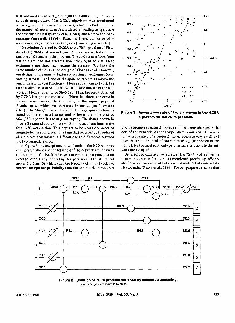
The solution obtained by GCSA to the 7SP4 problem of Flou- das et al. (1986) is shown in Figure 2. There are six hot streams and one cold stream in the problem. The cold stream flows from left to right and hot streams flow from right to left. Heat exchangers are shown connecting the streams. We have the same number of units as the design of Floudas et al. However, our design has the unusual feature of placing an exchanger (connecting stream 2 and one of the splits on stream 1) across the pinch. Using the cost function of Floudas et al., our network has an annualized cost of $644,480. We calculate the cost of the network of Floudas et al. to be $645,695. Thus, the result obtained by GCSA is slightly lower in cost. (Note that there is an error in the exchanger areas of the final design in the original paper of Floudas et al. which was corrected in errata (see literature cited). The $645,695 cost of the final design quoted above is based on the corrected areas and is lower than the cost of $647,050 reported in the original paper.) The design shown in Figure 2 required approximately 400 minutes of cpu time on the Sun 3/50 workstation. This appears to be about one order of magnitude more computer time than that required by Floudas et al. (A direct comparison is difficult due to differences between the two computers used.)

In Figure 3, the acceptance rate of each of the GCSA moves enumerated above and the total cost of the network are shown as a function of Ts,,. Each point on the graph corresponds to an average over many annealing temperatures. The structural moves ( I , 2 and 5) which alter the topology of the network are lower in acceptance probability than the parametric moves (3,4

----! 288.8 392.3 401.4 491.3 10.7 1 - 16.6

A * 0.71 O A

338.9

505.6

3 I Y.4

0.61 * I

o *

5.9

I

-2 402.9 630.6

- - 583.3

~

- - 433.4 496.8 555.6

- -

0.4

x x x

0.1

' 5

6

447.2 494.4

- - 31 1.1

- - 383.3 422.2 7

-

X

X

X

1. 4 0

2 0 5 x

3 6 6 * x

I I I I 1 A06 1 2 3 4 5

~ ~ ~ $ 1 0 4

algorithm for the 7SP4 problem. Figure 3. Acceptance rate of the six moves in the GCSA

and 6) because structural moves result in larger changes in the cost of the network. As the temperature is lowered, the acceptance probability of structural moves becomes very small and over the final one-third of the values of T, (not shown in the figure), for the most part, only parametric alterations to the network are accepted.

As a second example, we consider the 7SP4 problem with a discontinuous cost function. As mentioned previously, off-the- shelf heat exchangers cost between 50% and 75% of custom fabricated units (Rubin et al., 1984). For our purposes, assume that

Figure 2. Solution of 7SP4 problem obtained by simulated annealing. Flow rates on splits are shown in boldface.


3

2

c1$104

1

C

I

I I I I I I I 50 100 150 200 250 300 350 1

Area(rn2)

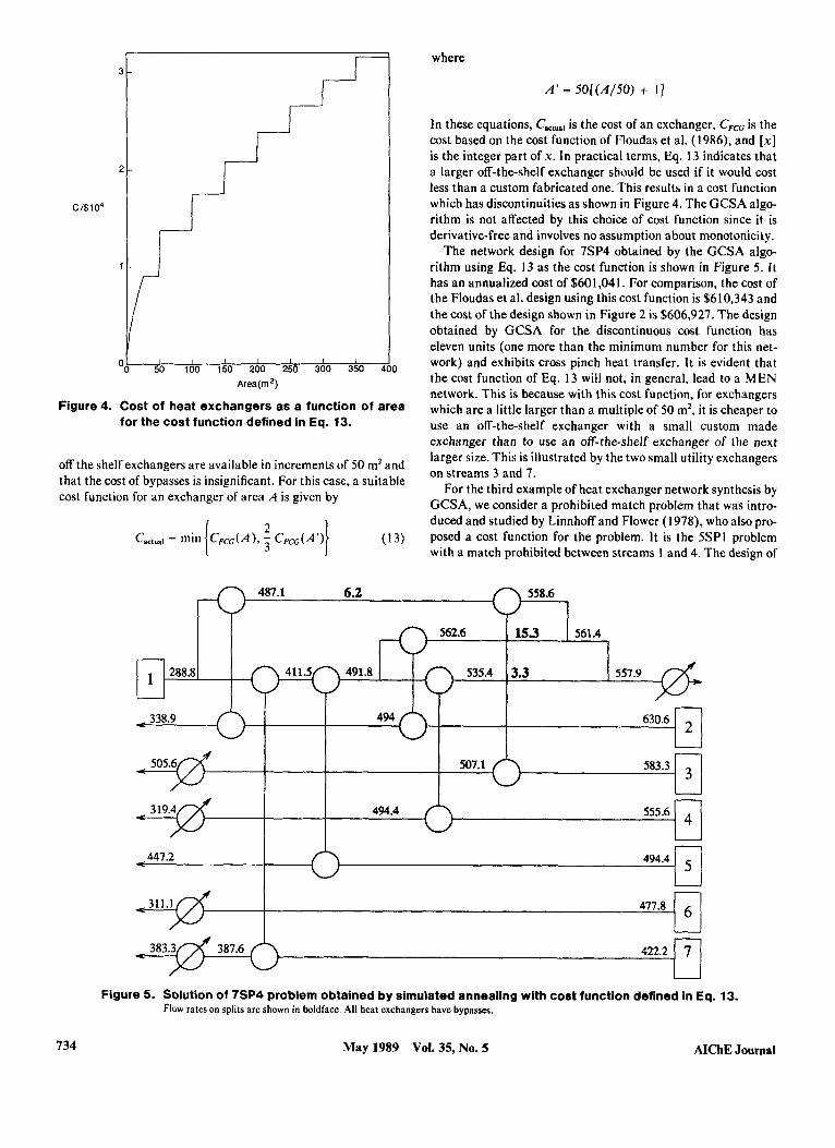
Figure 4. Cost of heat exchangers as a function of area for the cost function defined in Eq. 13.

off the shelf exchangers are available in increments of 50 m2 and that the cost of bypasses is insignificant. For this case, a suitable cost function for an exchanger of area A is given by

where

A' = 50[(A/50) -I- I ]

In these equations, C,,,,,, is the cost of an exchanger, CFcG is the cost based on the cost function of Floudas et al. ( 1 986), and [XI is the integer part of x. In practical terms, Eq. 13 indicates that a larger off-the-shelf exchanger should be used if it would cost less than a custom fabricated one. This results in a cost function which has discontinuities as shown in Figure 4. The GCSA algorithm is not affected by this choice of cost function since it is derivative-free and involves no assumption about monotonicity.

The network design for 7SP4 obtained by the GCSA algorithm using Eq. I3 as the cost function is shown in Figure 5. It has an annualized cost of $601,041. For comparison, the cost of the Floudas et al. design using this cost function is $61 0,343 and the cost of the design shown in Figure 2 is $606,927. The design obtained by GCSA for the discontinuous cost function has eleven units (one more than the minimum number for this network) and exhibits cross pinch heat transfer. It is evident that the cost function of Eq. 13 will not, in general, lead to a MEN network. This is because with this cost function, for exchangers which are a little larger than a multiple of 50 m2, it is cheaper to use an off-the-shelf exchanger with a small custom made exchanger than to use an off-the-shelf exchanger of the next larger size. This is illustrated by the two small utility exchangers on streams 3 and 7.

For the third example of heat exchanger network synthesis by GCSA, we consider a prohibited match problem that was introduced and studied by Linnhoff and Flower (1978), who also proposed a cost function for the problem. It is the 5SP1 problem with a match prohibited between streams I and 4. The design of

487.1 6.2 558.6

15.3 561.4

- 535.4 3.3 557.9 1 288.8

I

494

I - -3

-4

583.3

- - 555.6

- - - 5 447.2 494.4

. - 477.8 6 - -

387.6 422.2 7 L

Figure 5. Solution of 7SP4 problem obtained by simulated annealing with cost function defined in Eq. 13. Flow rates on splits are shown in boldface. A11 heat exchangers have bypasses.


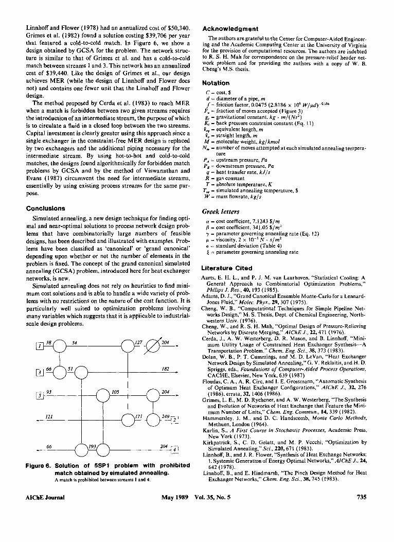
Linnhoff and Flower (1978) had an annualized cost of $50,340. Grimes et al. ( 1 982) found a solution costing $39,706 per year that featured a cold-to-cold match. In Figure 6, we show a design obtained by GCSA for the problem. The network structure is similar to that of Grimes et al. and has a cold-to-cold match between streams 1 and 3. This network has an annualized cost of $39,440. Like the design of Grimes et al., our design achieves MER (while the design of Linnhoff and Flower does not) and contains one fewer unit that the Linnhoff and Flower design.

The method proposed by Cerda et al. (1983) to reach MER when a match is forbidden between two given streams requires the introduction of an intermediate stream, the purpose of which is to circulate a fluid in a closed loop between the two streams. Capital investment is clearly greater using this approach since a single exchanger in the constraint-free MER design is replaced by two exchangers and the additional piping necessary for the intermediate stream. By using hot-to-hot and cold-to-cold matches, the designs found algorithmically for forbidden match problems by GCSA and by the method of Viswanathan and Evans (1987) circumvent the need for intermediate streams, essentially by using existing process streams for the same purpose.

93 5

121 *

Conclusions Simulated annealing, a new design technique for finding opti-

mal and near-optimal solutions to process network design problems that have combinatorially large numbers of feasible designs, has been described and illustrated with examples. Prob- lems have been classified as ‘canonical’ or ‘grand canonical’ depending upon whether or not the number of elements in the problem is fixed. The concept of the grand canonical simulated annealing (GCSA) problem, introduced here for heat exchanger networks, is new.

Simulated annealing does not rely on heuristics to find minimum cost solutions and is able to handle a wide variety of problems with no restrictions on the nature of the cost function. It is particularly well suited to optimization problems involving many variables which suggests that it is applicable to industrial- scale design problems.

105

182 -

66 *

Figure 6. Solution of 5SP1 problem with prohibited match obtained by simulated annealing. A match is prohibited between streams 1 and 4.

Acknowledgment The authors are grateful to the Center for Computer-Aided Engineer-

ing and the Academic Computing Center at the University of Virginia for the provision of computational resources. The authors are indebted to R. S. H. Mah for correspondence on the pressure-relief header network problem and for providing the authors with a copy of W. B. Cheng’s M.S. thesis.

Notation c = cost, $ d = diameter of a pipe, m /= friction factor, 0.0475 (2.8186 x 10’ W/pd)-0.’86

Fa - fraction of moves accepted (Figure 3) gc = gravitational constant, kg . m / ( N s 2 ) Ki = back pressure constraint constant (Eq. 11) P, - equivalent length, m Q, - straight length, m M - molecular weight, kglkmol N, - number of moves attempted at each simulated annealing tenipera-

PA = upstream pressure, Pa P, = downstream pressure, Pa q - heat transfer rate, k J / s R - gas constant T = absolute temperature, K

T,a = simulated annealing temperature, $ W - mass flowrate, kg/s

ture

Greek letters a = cost coefficient, 7.1243 $/m a - cost coefficient, 341.05 $/m2 y = parameter governing annealing rate (Eq. 12) p - viscosity, 2 x lo-’ N . s/m’ (r = standard deviation (Table 4) ( = parameter governing annealing rate

Literature Cited Aarts, E. H. L., and P. J . M. van Laarhoven, “Statistical Cooling: A

General Approach to Combinatorial Optimization Problems,” Philips J . Res.. 40, 193 (1985).

Adams, D. J., “Grand Canonical Ensemble Monte-Carlo for a Lennard- Jones Fluid,” Molec. Phys.. 29, 307 (1975).

Cheng, W. B., “Computational Techniques for Simple Pipeline Net- works Design,” M. S. Thesis, Dept. of Chemical Engineering, North- western Univ. (1976).

Cheng, W., and R. S. H. Mah, “Optimal Design of Pressure-Relieving Networks by Discrete Merging,” AIChE J., 22,471 (1976).

Cerda, J., A. W. Westerberg, D. R. Mason, and B. Linnhoff, “Mini- mum Utility Usage of Constrained Heat Exchanger Synthesis-A Transportation Problem,” Chem. Eng. Sci.. 38, 373 (1983).

Dolan, W. B., P. T. Cummings, and M. D. LeVan, “Heat Exchanger Network Design by Simulated Annealing,” G. V. Reklaitis, and H. D. Spriggs, eds., Foundations of Computer-Aided Process Operations, CACHE, Elsevier, New York, 639 (1987).

Floudas, C. A., A. R. Circ, and 1. E. Grossmann, “Automatic Synthesis of Optimum Heat Exchanger Configurations,” AIChE J. , 32, 276 (1986), errata, 32, 1406 (1986).

Grimes, L. E., M. D. Rychener, and A. W. Westerberg, “The Synthesis and Evolution of Networks of Heat Exchange that Feature the Mini- mum Number of Units,” Chem. Eng. Commun., 14,339 (1982).

Hammersley, J . M., and D. C. Handscomb, Monte Carlo Mefhods, Methuen, London (1 964).

Karlin, S., A First Course in Stochastic Processes, Academic Press, New York (1973).

Kirkpatrick, S., C. D. Gelatt, and M. P. Vecchi, “Optimization by Simulated Annealing,” Sci., 220,671 (1983).

Linnhoff, B., and J. R. Flower, “Synthesis of Heat Exchange Networks: 1. Systemic Generation of Energy Optimal Networks,” AIChE J. . 24, 642 ( 1 978).

Linnhoff, B., and E. Hindmarsh, “The Pinch Design Method for Heat Exchanger Networks,” Chem. Eng. Sci.. 38,745 (1983).


Linnhoff, B., and J. A. Turner, “Heat Exchanger Networks: New Insights Yield Big Savings,” Chem. Eng., 88(22), 56 (1981).

Lundy, M., and A. Mees, “Convergence of the Annealing Algorithm,” Simulated Annealing Workshop, Yorktown Heights (Apr., 1984).

Martin, D. L., and J. L. Gaddy, “Process Optimization with the Adap- tive Randomly Directed Search,” AIChE Symp. Ser., 78(214), 99 (1982).

Metropolis, N., A. Rosenbluth, M. Rosenbluth, A. Teller, and E. Teller, “Equation of State Calculations by Fast Computing Machines,” J. Chem. Phys., 21, 1087 (1953).

Murtagh, B. A,, “An Approach to the Optimal Design of Networks,” Chem. Eng. Sci., 27, 1131 (1972).

Papoulias, S. A., and 1. E. Grossmann, “A Structural Optimization Approach in Process Synthesis: II. Heat Recovery Networks,” Comp. Chem. Eng.. 7,707 (1983).

Press, W. H., B. P. Flannery, W. T. Teukolsky and W. T. Vetterling, “Numerical Recipes: the Art of Scientific Programming,” Cam- bridge University Press, Cambridge (1986).

Romeo, F., and A. Sangiovanni-Vincentelli, “Probabilistic Hill Climb- ing Algorithms: Properties and Applications,” ERL, College of Engi- neering, Univ. of California, Berkeley (1 984).

Rubin, F. L., H. A. Moak, A. D. Holt, F. C. Standiford, and D. Stuhl- barg, “Heat-Transfer Equipment” R. H. Perry and D. Green, eds., Perry’s Chemical Engineers’ Handbook. McGraw-Hill, New York, 1 1 (1964).

Rothfarb, B., H. Frank, D. M. Rosenbaum, K. Steiglitz, and D. J. Kleit- man, “Optimal Design of Offshore Natural-Gas Pipeline Systems,” Oper. Res.. 18,992 (1 970).

Snook, I. K., and W. van Megen, “Calculation of Solvation Forces between Solid Particles Immersed in a Simple Fluid,” J. Chem. SOC. Farad. Trans. 11, 77, 181 (1981).

Valleau, J. P., and S. G. Whittington, “A Guide to Monte Cario for Sta- tistical Mechanics: 1. Highways,” B. J. Berne, ed., Modern Theoreti- cal Chemistry: 5 . Statistical Mechanics. Plenum Press, New York, 134 (1977).

Viswanathan, M., and Evans, L. B., “Studies in the Heat Integration of Chemical Process Plants,” AZChE J. . 33, 1781 (1987).

Wohlpart, D., “Design of Pipe Networks by Simulated Annealing,” Univ. of Virginia, unpublished (1987).

Manuscript received Aug. 2, 1988, and revision received Dec. 29,1988.

736 May 1989 Vol. 35, No. 5 AiChE Journal

process optimization via simulated annealing:...

Documents