Procurement design with corruption

Roberto Burguet∗

Institute for Economic Analysis (CSIC) and Barcelona GSE

This version: March, 2015

Abstract

This paper investigates the design of optimal procurement mechanisms in thepresence of corruption. After the sponsor and the contractor sign the contract,the latter may bribe the inspector to misrepresent quality. Thus, the mechanismaffects whether bribery occurs. I show how to include bribery as an additionalconstraint in the optimal-control problem that the sponsor solves, and charac-terize the optimal contract. I discuss both the case of fixed bribes and bribesthat depend on the size of the quality misrepresentation, and also uncertaintyabout the size of the bribe. In all cases, the optimal contract curtails qualitynot only for low effi ciency contractors but also for the most effi cient contractors.Implementation is also discussed.Keywords: bribery; quality; contract designJEL numbers: D82, D73, H57

1 Introduction

There has been growing interest in recent years in both the economic effects of corrup-

tion and also potential remedies for dealing with it. Corruption ranks high among the

diffi culties when organizing procurement in general and public procurement in partic-

ular.1 Indeed, offi cials and contractors are often tempted by the gains from trading

∗Indranil Chakraborty is responsible for my interest in this problem. I thank him for having spenttime working with me on it. I also thank audiences in U. of Illinois, U. of North Carolina, Duke U.,Michigan State U., U. of Cologne, XXIX JEI, EARIE 2014, CEME2014, AMES2014, IO Workshopin Hangzhou, and Procurement Workshop in Rio de Janeiro. Finally, I acknowledge financial supportfrom the Spanish Ministry of Science and Innovation (Grant: ECO2011-29663), and the Generalitatde Catalunya (SGR 2014-2017).

1As an example, according to the Minister for State-Owned Enterprises, 80% of corruption andfraud in state-owned Indonesian companies occur in public procurement. (Transparency International,2006.)

1

in illegal, or at least illegitimate, mutual favors. Bribes are often exchanged for ma-

nipulation of either the rules that select the price (and/or identity of the contractor)

or the quality of the good delivered. In this paper, I study the design of optimal

procurement mechanisms for the principal (sponsor) in the face of this latter form of

manipulation.2 I begin by showing that standard tools in mechanism design may be

adapted to characterize and analyze this problem. As we discuss below, the effect of

this sort of corruption is to transform an adverse selection problem into an adverse-

selection/moral-hazard problem to which standard tools may be applied.

Consider the standard procurement design problem, where the principal cares about

quality and price, and the cost of delivering quality is the contractor’s private infor-

mation. Quality cannot be directly observed, and the contract supervisor or inspector

in charge of assessing delivered quality can be "bought". In the simplest bribe model,

this can be done by paying a fixed bribe. The key, simple observation is that a (direct)

mechanism may then be defined as a triple of functions that specifies not only the qual-

ity and the price for each ’type’of contractor, but also whether the contractor should

bribe or not. This is the moral hazard dimension that bribery introduces. As with

collusion-proofness (see Tirole, 1986), dealing with corruption then adds a new incen-

tive compatibility constraint to the sponsor’s choice. In this case, the constraint that

guarantees that the contractor does not have incentives to disregard the instruction

with respect to bribing.

I characterize optimal mechanisms in this scenario and show that bribing imposes

a bound on the levels and range of quality that are implementable. In response, the

principal gives up inducing any (non-trivial) quality for an interval at the low-effi ciency

tail of types. This is probably not surprising. What is more subtle is that bribery is

also problematic at the other end of the type domain. Indeed, due to the possibility

of bribing, the sponsor optimally curtails the quality that it contracts with the most

effi cient contractors. Obtaining higher quality from these types obviously requires

2Transparency International lists this as one of the four areas of increased risk in the procurementcycle, together with limited access to information, abuse of exceptions and the budget phase. SeeTransparency International (2006).

2

promising them a higher price. That, in turn, makes it more attractive for low-effi ciency

types to bribe the inspector in order to (claim high effi ciency and so) contract high

quality, while delivering less of it. Therefore, the higher the quality contracted with

high-effi ciency types the tighter the incentive constraint for lower-effi ciency types.

Note that this incentive constraint is not local, but global. Indeed, bribing allows

a contractor to target the highest price while avoiding the cost of delivering the corre-

sponding highest quality. Thus, conditional on bribing, a contractor would (contract

highest quality, i.e., would) claim to be the highest effi ciency type.

When the cost of manipulation, i.e., the size of bribe, is fixed and common knowl-

edge, the possibility of bribery binds, but bribery does not occur when the sponsor

designs the optimal mechanism. The same would be true if there was uncertainty

about the size of the required bribe, but the uncertainty was resolved only after the

project had been completed. However, things are different if the uncertainty about the

required bribe was resolved after contracting but before the project was completed.

This is the case if, for instance, the identity (and inclination to gift exchanges) of the

contract supervisor is revealed only after the contract is signed. Completely preventing

bribery may not be in the sponsor’s interest in that case. I characterize the optimal

mechanism under this alternative model. In that mechanism, no type bribes with

probability one, but bribery may occur with positive probability for all types. Indeed,

after quality is contracted and the size of the required bribe learnt by the contractor,

the contractor will always choose whatever is cheaper: bribing or delivering. If the

necessary bribe happens to be very small, bribing will be cheaper than delivering any

non trivial quality. Thus, bribery can be seen as a modification of the contractor’s

cost function. Other than that, the problem is technically very similar to the design

problem in the absence of corruption. The effect of bribery is that, again, the sponsor

optimally gives up inducing the low tail of effi ciency types to deliver quality, and con-

tracts lower quality with all types of contractor, even the most effi cient one. In that

sense, the effect of bribery is similar whether bribes are paid or not in equilibrium.

I also consider the case where the size of the bribe depends on the size of manipu-

lation obtained from the inspector. If the required bribe is (suffi ciently) concave in the

3

size of manipulation, the conclusions are similar to the known, fixed-bribe case. Indeed,

a fixed bribe may be thought of as an extreme example of a concave bribe. Under suf-

ficient concavity, the conclusions of the model are not affected: moral-hazard incentive

compatibility is binding for the lowest effi ciency types who may imitate the highest

effi ciency type (a global constraint). No bribes are paid in the optimal mechanism,

and quality is curtailed at both ends of the type distribution.

The convex case, on the contrary, is similar to the fixed but uncertain bribe case. In

particular, if the marginal cost of bribing is very low for very low levels of manipulation,

all types will find it attractive to ’buy’some manipulation instead of delivering all the

contracted quality. As a result, bribery for all types will also be part of the outcome of

the optimal mechanism. Under some assumptions on the convexity of the bribe, this

again is akin to a modification of the contractor’s cost function.

The shape of the ’bribe’, i.e., of the cost that bribing represents for the contractor

may be determined by social traits. Indeed, different societies are characterized by

different degrees of the incidence and tolerance of corruption.3 When it is very costly

to lure an offi cial into illegal transactions, bribes are naturally concave in the amount

of manipulation. A moderate bribe may be ineffective to induce the offi cial to cross the

line, but once crossed it makes sense to make the effort worthwhile. Contrary, when

graft is widely practiced and viewed as acceptable to some degree, bribes are better

represented as convex in the size of manipulation. Small manipulation is probably safe,

but even if the rule is to break the rule there are norms as to what does it mean to

really break rules.4

After characterizing optimal mechanisms, I study implementation, and show that

a simple menu of contracts, much in the spirit of Che (1993), does implement optimal

procurement.

3Several theories have been proposed to explain differences in the prevalence of corruption insocieties, both based on ’rational’behavior (e.g., based on reputation, cf. Tirole, 1996; or multiplicityof equlibria, c.f., Acemoglu, 1995) and on ’social norms’. In their study of the empirical relationshipbetween inequality and corruption, You and Khagram (2005) argue that social norms and perceptionsis a chanel through which inequality affects corruption.

4Truex (2011) reports the results of a survey of Kathmandu residents that shows that respondentsgenerally agree that large-scale bribery was unacceptable, but also that petty corruption, gift giving,and favoritism are much more acceptable.

4

Finally, I consider competition. That is, I allow for the presence of several, symmet-

ric contractors capable of undertaking the sponsor’s project. Typically, competition

does not affect the choice of quality as a function of the contractor’s type, although it

does reduce the expected price for the sponsor conditioning on quality. This is still the

case when corruption introduces only locally binding incentive constraints. Indeed, as

we have noted, both in the uncertain and fixed bribe and in the convex bribe cases

corruption is equivalent to a modification of the contractors’ cost function. This is

unaffected by the number of potential contractors, and so bribery does not affect this

optimal relationship between quality and type. However, when the bribe is fixed and

known or concave, and so optimal procurement calls for avoiding bribes, things are

more subtle. Indeed, in these cases the fact that competition reduces the price that is

necessary for obtaining high quality from high effi ciency types implies that competi-

tion reduces the incentives for low effi ciency types to imitate high effi ciency ones. The

result is that competition relaxes the global constraint imposed by corruption. Conse-

quently, competition alleviates the quality distortion for high effi ciency types. That is,

competition not only reduces the price of quality for the sponsor but also allows the

sponsor to obtain higher levels of quality from the same type of contractor.

One technical contribution of this paper is to solve a problem where incentive

constraints bind not only locally. As we have noted before, in the fixed and concave

bribe cases, incentive compatibility related to moral hazard (no bribing) means that

no type should have incentives to imitate the most effi cient. This constraint is most

stringent for the least effi cient type. The strategy that I follow for characterizing the

optimal mechanism is to fix an arbitrary quality for the most effi cient type. Given

this arbitrary value, I then characterize the sponsor’s problem as a free-time, fixed-

endpoint control problem. The optimal mechanism is the solution to this problem

when the quality selected for the most effi cient type is also optimal. That is, when

the sponsor’s surplus in the solution to the optimal control problem is maximized with

respect to that quality.

Corruption has received much attention in the economic literature at least since

Rose-Ackerman (1975) pioneering paper. (See Aidt, 2003, for a survey.) On the effects

5

of corruption on procurement, auction theorists have sought to understand how ma-

nipulation and bribe-taking affect the allocation and surplus-sharing when particular

mechanisms are used to allocate contracts or goods. The literature has studied specific

ways (typically, bid readjusment) in which an agent acting on behalf of the principal

may, in exchange for a bribe, favor a contractor in some particular auction mechanism.

(See, among other, Lambert-Mogiliansky, and Verdier, 2005, Menezes and Monteiro,

2006, Burguet and Perry, 2007, Koc and Neilson, 2008, Arozamena and Weinschel-

baum, 2009, or Lengwiler and Wolfstetter, 2010.) The literature has also considered

the effects of manipulation when quality, and not only price, is an argument in the

principal’s objective function. (See Celentani and Ganuza, 2002, and Burguet and

Che, 2004.) With the exception of Celentani and Ganuza (2002), in all these papers

the agent’s ability to manipulate is defined in reference to the particular mechanism

itself. Thus, the analysis of remedies is limited in scope, and for good reason: the mere

question of what is an optimal mechanism from the principal’s point of view may be

ill-defined in these settings. For example, assume that an agent in charge of running

a sealed-bid, first-price procurement auction is able to learn the bids before they are

publicly opened, and is also able to adjust downward one of the contractors’bid, if

that bid is not already the lowest. This is the model studied in most of the papers

previously mentioned. If instead, the procurement mechanism was an oral auction,

this ability would be irrelevant. Even in a second-price auction, altering one contrac-

tor’s bid would be of no value to that contractor. Perhaps in either of these other

auction formats the agent may manipulate the outcome by other means. The question

would then become what is the ’equivalent’to bid readjustment in those, or any, other

auction formats? That is, the question of what constitutes an optimal procurement

format, in the presence of corruption, takes us to a more complex problem: defining

what a corrupt procurement agent may do under each of the possible mechanisms the

principal may design.5

5Note that, if the corrupt agent’s ability to bend the rules depends on the rules themselves, theproblem for the principal is not one where standard tools in mechanism design may be used. Eventhe revelation principle is problematic, as equivalence of mechanisms cannot be predicated withoutreference to equivalence of manipulation. That is, given the lack of a simple way of establishing

6

To my knowledge, this is the first paper that investigates the design of procure-

ment mechanisms in the presence of bribery when the mechanism affects the incidence

of bribery. Note that, contrary to many of the papers cited in the previous paragraph,

I consider corruption in the execution of the contract, not in the negotiation of its

terms. This means that the design of the procurement mechanim may affect the in-

cidence of corruption, but what manipulation means can be defined independent of

the mechanism itself. In their insightful paper, Celentani and Ganuza (2002) do study

the optimal mechanism with a corrupt agent who may (adjust bids and) misrepresent

quality assessment. However, (potential) corrupt deals pre-date the principal’s choice

of mechanism, and so the mechanism cannot affect quality, if corrupt deals indeed took

place. Moreover, the authors assume that information rents are determined as in the

absence of bribery, justifying this assumption on the need for ’hiding’corrupt deals.

Under these assumptions, the sponsor knows that she will pay for quality as if no cor-

ruption existed, but will obtain that quality with a fixed, exogenous probability lower

than one. Therefore, the sponsor optimally induces lower quality from all types: the

optimal mechanisms coincides with the optimal mechanism in the absence of bribery

when quality is multiplied by a constant equal to that exogenous probability of actually

getting the contracted quality.

In the next section, I present the basic model with a fixed bribe and obtain the

optimal mechanism for this case. Section 3 introduces uncertainty concerning the size

of the bribe and characterizes the optimal mechanism for that case. In Section 4,

I let the size of the bribe be a function of the amount of manipulation, and obtain

conclusions both for the (suffi ciently) concave and convex cases. Section 5 discusses

implementation of the optimal procurement rules, and Section 6 discusses the effects

of an increase in competition. Some concluding remarks close the paper. An appendix

contains all proofs.

equivalence classes in the set of mechanisms, restricting attention to revelation games may simply beof no use.

7

2 The model

A sponsor procures a contract of fixed size and variable quality, q ∈ [0,∞). Quality q

measures the sponsor’s willingness to pay for the project. That is, the payoff for the

sponsor when she pays P and receives a project with realized quality q is simply q−P .

The sponsor’s goal is to maximize the expected value of that payoff.

A contractor is able to undertake the project and deliver quality q at a cost C(q; θ),

where θ ∈ [θ, θ] is the contractor’s type and her private information. From the sponsor’s

point of view, θ is the realization of some random variable with cdf F and density f in

[θ, θ], and this is common knowledge. We postulate a differentiable C with Cθ, Cq > 0,

and Cqθ, Cqq > 0. This guarantees that, in the absence of bribery, monotonicity of q

with respect to θ is virtually all that is needed for implementation. Also, we assume

that C(0; θ) = 0, for all θ, and that

Cq(q; θ) + Cqθ(q; θ)F (θ)

f(θ)(1)

is increasing both in q and in θ. This guarantees interior (to monotonicity constraints)

solution for the optimal mechanism in the absence of bribery. (See Che, 1993.)

Zero quality should be interpreted as a standard minimum quality, and a positive

quality as quality obtained at an additional cost to the contractor. Likewise, a price of

zero corresponds to a payment that equals the (common) cost of honoring the contract

at a standard, minimum quality, q = 0.

Under observability of quality, and so without any role for the inspector, a direct

mechanism is a pair (p, q), where p : [θ, θ]→ R and q : [θ, θ]→ R+. p(θ) represents the

payment that the contractor gets and q(θ) represents the quality that the contractor

provides. Both are functions of the contractor’s type. The sponsor needs to consider

only incentive compatible, individually rational, direct mechanisms. Among them, the

optimal one is characterized by quality qNB(θ) that satisfies

1− Cq(qNB(θ); θ)− Cqθ(qNB(θ); θ)F (θ)

f(θ)= 0. (2)

as long as

qNB(θ)− C(qNB(θ); θ) ≥ Cθ(qNB(θ); θ)

F (θ)

f (θ), (3)

8

and qNB(θ) = 0 otherwise. (See Che, 1993.) In order to simplify the analysis and

also concentrate on the interesting results below, we will assume that (3) holds with

equality when evaluated at θ and qNB(θ) = 0 so that qNB(θ) > 0, for all θ < θ.6

In this paper, we are interested in analyzing the case when quality q is not directly

observable. Instead, the sponsor requires an agent, the inspector, who assesses (or

certifies) the quality of the completed project. The inspector can observe q without

cost.

The inspector can also accept bribes to be untruthfulwhen reporting on quality.

For now, we assume that the agent will do so in exchange for a fixed bribe B. In later

sections we will consider more general specifications of B.7 In any case, we should note

that the bribe B includes any (expected) payment by the contractor associated with

bribing the agent.

Under the threat of bribery, we may define a direct mechanism as a triple (p, q, b),

where p and q are defined and interpreted as above, and b : [θ, θ]→ {0, 1}. We interpret

b(θ) = 1 as an instruction to bribe and b(θ) = 0 as an instruction not to bribe. Also,

we should interpret q(θ) as the contracted quality, not necessarily the delivered one.8

Let

Π(θ) = b(θ) (p(θ)−B) + (1− b(θ)) (p(θ)− C(q(θ); θ))

The mechanism is implementable if it satisfies incentive compatibility (IC) and

individual rationality (IR), as in any standard problem:

IR) For all θ ∈ [θ, θ], Π(θ) ≥ 0.

IC) For all θ, z ∈ [θ, θ], Π(θ) ≥ p(z)−min {C(q(z); θ), B}.

Incentive compatibility incorporates adverse selection and moral hazard constraints.

6If (3) is negative at θ for q = 0, everything that follows applies with only redefining the domainof types to the interval where (3) is non negative. Also, if (3) is strictly positive at θ and for q = 0,then the value of θc defined later may be equal to, not strictly smaller than, θ. That "corner" solutionwould not affect any other insight.

7In all cases, we do not consider the possibility of "extortion", that is, the possibility that theinspector asks for bribes in order to report the truth, threatening to otherwise report lower qualitythan what is actually delivered. Note that in this type of corrupt behavior the parties involved,inspector and contractor, have conflicting interest. This is contrary to the cases studied in this paper.

8For the moment, we do not need to specify delivered quality: if b(θ) = 1, then delivered qualitywill be 0, and otherwise it will be q(θ).

9

In particular, for b(θ) = 0, Π(θ) ≥ p(θ) − B. That is, the contractor’s profits should

be at least as large as the profit she could get by simply bribing. Note that incentive

compatibility implies that if b(θ) = 1, then delivered quality will be 0, and so we do

not need to specify delivered quality when b(θ) = 1.

The problem for the sponsor is to design the direct, implementable mechanism

(p, q, b) that maximizes her expected payoff, E [q(θ)(1− b(θ))− p(θ)].

When the bribe B is known and fixed, that optimal mechanism cannot include

an instruction to bribe for any type of contractor. The contractor would still have

incentives to report truthfully her type if, instead, the mechanism asked her to deliver

0 quality and offered her a price of p(θ)−B. The sponsor can thus get the same quality

for a lower price. Indeed,

Lemma 1 For any IC, IR direct mechanism, (p, q, b), there exists an IC, IR mecha-

nism with b(θ) = 0 ∀θ ∈ [θ, θ], so that E [q(θ)(1− b(θ))− p(θ)] is higher for the latter.

Thus, in this basic setting, bribery does not occur in the optimal mechanism, so

we can restrict attention to mechanisms with b(·) = 0, but bribery does still impose

restrictions on mechanisms for IC and IR to hold.

In particular, standard necessary conditions for IC and IR (under no bribery) are

still necessary. Indeed, even without intending to bribe the inspector, the contractor

should have incentives to report her type truthfully. Three consequences follow from

these necessary conditions. First, Π(θ) must be monotone decreasing. In fact,

π(z; θ) ≡ p(z)− C(q(z); θ)

satisfies the conditions of Theorem 2 in Milgrom and Segal (2002), so that

Π(θ) = p(θ)− C(q(θ); θ) = Π(θ) +

θ∫θ

Cθ(q(z); z)dz, (4)

and is absolutely continuous. That virtually fixes p(θ) as a function of q(θ). Second,

and as a result, a necessary but also suffi cient condition for IR is Π(θ) ≥ 0. Third,

monotonicity can also be extended to q and p in a standard way.

10

Lemma 2 In any IC mechanism, p(θ) and q(θ) are monotone decreasing.

These features, which are shared by any feasible mechanism in the absence of cor-

ruption, have important consequences that make this problem tractable. Indeed, since

p is monotone, a bribing contractor of any type would maximize profits by claiming

type θ. Also, since Π is monotone, type θ is the type with the strongest incentives to

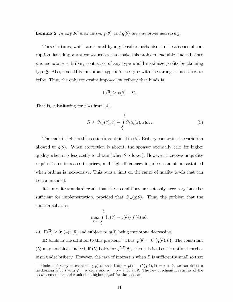
bribe. Thus, the only constraint imposed by bribery that binds is

Π(θ) ≥ p(θ)−B.

That is, substituting for p(θ) from (4),

B ≥ C(q(θ); θ) +

θ∫θ

Cθ(q(z); z)dz. (5)

The main insight in this section is contained in (5). Bribery constrains the variation

allowed to q(θ). When corruption is absent, the sponsor optimally asks for higher

quality when it is less costly to obtain (when θ is lower). However, increases in quality

require faster increases in prices, and high differences in prices cannot be sustained

when bribing is inexpensive. This puts a limit on the range of quality levels that can

be commanded.

It is a quite standard result that these conditions are not only necessary but also

suffi cient for implementation, provided that Cqθ(q; θ). Thus, the problem that the

sponsor solves is

maxp,q

θ∫θ

{q(θ)− p(θ)} f (θ) dθ,

s.t. Π(θ) ≥ 0; (4); (5) and subject to q(θ) being monotone decreasing.

IR binds in the solution to this problem.9 Thus, p(θ) = C(q(θ), θ

). The constraint

(5) may not bind. Indeed, if (5) holds for qNB(θ), then this is also the optimal mecha-

nism under bribery. However, the case of interest is when B is suffi ciently small so that

9Indeed, for any mechanism (q, p) so that Π(θ) = p(θ) − C(q(θ), θ

)= ε > 0, we can define a

mechanism (q′, p′) with q′ = q and q and p′ = p − ε for all θ. The new mechanism satisfies all theabove constraints and results in a higher payoff for the sponsor.

11

(5) does bind. The following proposition characterizes the optimal mechanism also for

this case

Proposition 3 If (5) holds for the optimal mechanism without bribery, qNB(θ), then

(qNB, pNB, b) with b(θ) = 0 for all θ, is the optimal mechanism under bribery. Other-

wise, there exist θa and θc, with θ < θa ≤ θc < θ such that at the optimal mechanism;

(i) q(θ) = 0 if θ > θc ; (ii) q(θ) = qNB(θ) if θ ∈ (θa, θc); and (iii) q(θ) = qNB(θa) if

θ < θa.

Thus, when the size of the bribe is fixed and known and bribery is a relevant

constraint, the sponsor gives up the possibility of obtaining (an increase in) quality

from contractors with very high costs. This result is not surprising. Indeed, recall that

bribery imposes a limit on the range of possible quality levels that can be commanded.

If the sponsor is going to shave this range, she optimally does so for types with low

effi ciency. The loss from such distortion is lowest when the contractor has one of these

types. But, perhaps less obviously, quality is optimally distorted also at the top, i.e.,

when the contractor has a high effi ciency.

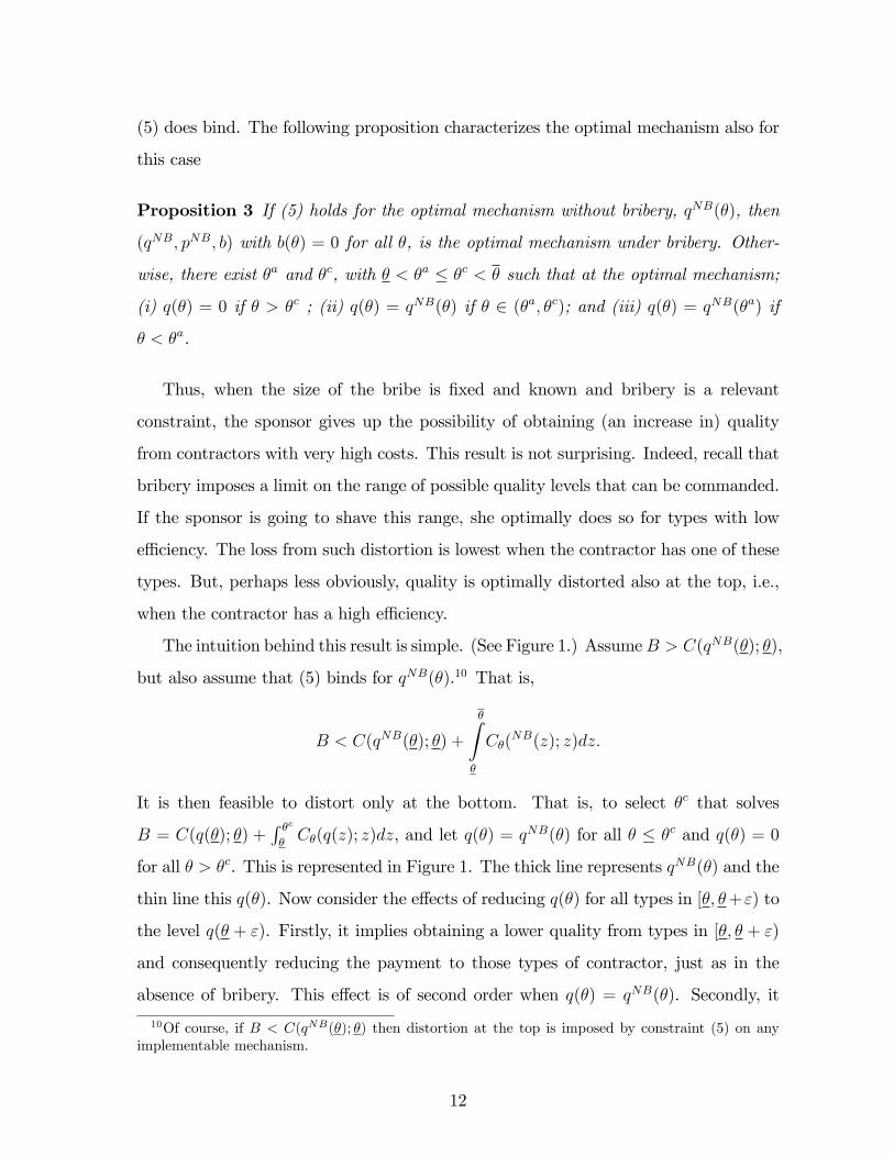
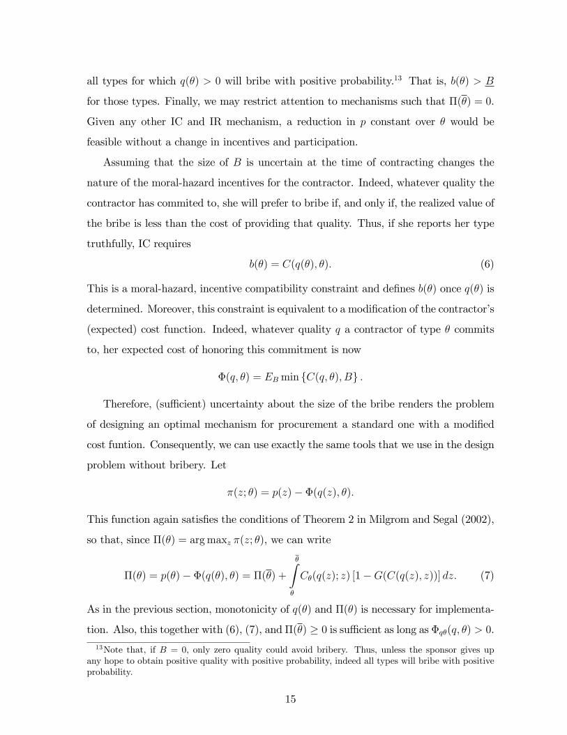
The intuition behind this result is simple. (See Figure 1.) AssumeB > C(qNB(θ); θ),

but also assume that (5) binds for qNB(θ).10 That is,

B < C(qNB(θ); θ) +

θ∫θ

Cθ(NB(z); z)dz.

It is then feasible to distort only at the bottom. That is, to select θc that solves

B = C(q(θ); θ) +∫ θcθCθ(q(z); z)dz, and let q(θ) = qNB(θ) for all θ ≤ θc and q(θ) = 0

for all θ > θc. This is represented in Figure 1. The thick line represents qNB(θ) and the

thin line this q(θ). Now consider the effects of reducing q(θ) for all types in [θ, θ+ε) to

the level q(θ + ε). Firstly, it implies obtaining a lower quality from types in [θ, θ + ε)

and consequently reducing the payment to those types of contractor, just as in the

absence of bribery. This effect is of second order when q(θ) = qNB(θ). Secondly, it

10Of course, if B < C(qNB(θ); θ) then distortion at the top is imposed by constraint (5) on anyimplementable mechanism.

12

also implies a more relaxed no-bribing constraint, as it is now less profitable to claim a

type θ when the type is in fact higher. That is, the reduction in q(θ) allows raising θc.

This is a first-order effect, as types that fall between the old and the new values of θc

can now be asked to supply quality qNB(θc) at a price C(q(θc); θc) instead of quality 0

at price 0. In other words, a reduction in q(θ) allows the contractor to expect positive

levels of quality from the previously marginal type θc. This effect is first-order, and

therefore distorting at the top is surplus improving for the sponsor.

q

θθ θ

)(θN Bq

∆q

∇q

qNB

Figure 1

3 Bribing in equilibrium

Perhaps the most interesting feature of the optimal mechanism discussed in the previous

section is that quality is distorted at the high end of the distribution of contractor types.

That is, bribery imposes a quality ceiling. However, the finding that bribery is not an

equilibrium phenomenon is a consequence of assuming that B, the size of the bribe, is

fixed and common knowledge, so that the sponsor should virtually ’buy’the possibility

of bribing. Suppose, instead, that B is uncertain at the time of contracting, and is only

learnt by the contractor after the terms of the contract have been set but before quality

13

is delivered.11,12 In particular, assume now that B takes values in some interval, [B,B]

according to some c.d.f. G with density g. We will make the standard assumption that1−G(B)g(B)

is decreasing in B.

To simplify the analysis, we may also assume that B is suffi ciently low, say B = 0.

(At the end of this section, we will comment on the consequence of not assuming so.)

Under these conditions, an optimal mechanism is not bribe-proof in general. Indeed,

preventing all types of contractor from bribing in all probability -when B is low- may

be too expensive for the sponsor.

Thus, we should now define a contract as a triple (p, q, b), where p : [θ, θ]→ R and

q : [θ, θ]→ R+, as before, and b : [θ, θ]→ [B,B]. b(θ) is now interpreted as the cut-off

value for B so that type θ is instructed to bribe if and only if B < b(θ). It is suffi cient

to consider mechanisms of this form. Indeed, if a contractor prefers not to bribe when

the size of the bribe is B, she will also prefer not to bribe when the size of the bribe is

larger than B. Contrary, if the contractor prefers to bribe when the size of the bribe

is B, then she also prefers to bribe if the size of the bribe is smaller than B. Thus, IC

will require that the instruction to bribe takes a cut-off form. Also, as in the previous

section, we do not have to specify what quality is to be delivered if bribing: IC requires

that quality to be 0.

As we have mentioned, in general, bribing will take place in equilibrium, but there

is still a counterpart to Lemma 1:

Lemma 4 For any IC and IR mechanism where at least one type θ bribes with proba-

bility 1, there is another IC and IR mechanism where no type bribes with probability 1

and results in (weakly) higher payoff for the sponsor.

Thus, we may restrict attention to mechanisms with b(θ) < B. Also, since B = 0,

11This would fit a case where the agent in charge of quality assessment is hired after the contracthas been signed. Note that, if the contractor privately learnt B before signing the contract, we wouldhave a standard mechanism-design problem where the contractor’s "type" would be (θ,B).12The case where uncertainty about B is resolved after the quality is delivered is equivalent to the

fixed and known B, with only substituting EB for B. Indeed, in that case the decision whether tobribe or not would have to be taken before providing quality. Not providing quality but claiming to doso would require the contractor to pay the bribe B whatever its realization, whereas if the contractorprovides quality there is no point in also paying the bribe.

14

all types for which q(θ) > 0 will bribe with positive probability.13 That is, b(θ) > B

for those types. Finally, we may restrict attention to mechanisms such that Π(θ) = 0.

Given any other IC and IR mechanism, a reduction in p constant over θ would be

feasible without a change in incentives and participation.

Assuming that the size of B is uncertain at the time of contracting changes the

nature of the moral-hazard incentives for the contractor. Indeed, whatever quality the

contractor has commited to, she will prefer to bribe if, and only if, the realized value of

the bribe is less than the cost of providing that quality. Thus, if she reports her type

truthfully, IC requires

b(θ) = C(q(θ), θ). (6)

This is a moral-hazard, incentive compatibility constraint and defines b(θ) once q(θ) is

determined. Moreover, this constraint is equivalent to a modification of the contractor’s

(expected) cost function. Indeed, whatever quality q a contractor of type θ commits

to, her expected cost of honoring this commitment is now

Φ(q, θ) = EB min {C(q, θ), B} .

Therefore, (suffi cient) uncertainty about the size of the bribe renders the problem

of designing an optimal mechanism for procurement a standard one with a modified

cost funtion. Consequently, we can use exactly the same tools that we use in the design

problem without bribery. Let

π(z; θ) = p(z)− Φ(q(z), θ).

This function again satisfies the conditions of Theorem 2 in Milgrom and Segal (2002),

so that, since Π(θ) = arg maxz π(z; θ), we can write

Π(θ) = p(θ)− Φ(q(θ), θ) = Π(θ) +

θ∫θ

Cθ(q(z); z) [1−G(C(q(z), z))] dz. (7)

As in the previous section, monotonicity of q(θ) and Π(θ) is necessary for implementa-

tion. Also, this together with (6), (7), and Π(θ) ≥ 0 is suffi cient as long as Φqθ(q, θ) > 0.

13Note that, if B = 0, only zero quality could avoid bribery. Thus, unless the sponsor gives upany hope to obtain positive quality with positive probability, indeed all types will bribe with positiveprobability.

15

This condition requires Cθ(q; θ) [1−G(C(q; θ))], and not only Cθ(q; θ), to be increasing

in q. It is satisfied, for instance, if B is disperse, so that g is small for any value of B.

The expected surplus for the sponsor can be written as

θ∫θ

{[1−G(C(q(θ), θ))] [q(θ)− C(q(θ), θ)]− Π(θ)} f(θ)dθ, (8)

where, in an IC mechanism, Π(θ) is given in (7). We are now ready to discuss the

optimal mechanism for the sponsor.

Proposition 5 There exists θd, with θ < θd ≤ θ such that at the optimal mechanism;

(i) q(θ) = 0 if θ > θd; and (ii) if θ < θd, then q(θ) solves

0 =1−G(C(q, θ))

g(C(q, θ))

{1− Cq(q, θ)− Cθq(q, θ)

F (θ)

f(θ)

}(9)

−Cq(q, θ){q − C(q, θ)− Cθ(q, θ)

F (θ)

f(θ)

}.

The intuition behind this result is relatively straightforward when considering the

Hamiltonian of the problem that the sponsor’s choice of q solves. Suppressing the

variables in the functions for compactness, this Hamiltonian is

H = (1−G(C)) [(q − C) f − FCθ] .

Note that in the absence of bribery, the corresponding Hamiltonian would be

HNB = (q − C) f − FCθ.

Thus,

H = (1−G(C))HNB.

The interpretation is simple. Quality q(θ) will be delivered with probability 1−G(C),

and then with that probability, the decision on q will have the same consequences on

contractor rents, cost, and sponsor surplus, as in the absence of bribery. This is the

phenomenon captured in Celentani and Ganuza (2002). In the present setting, this

would have no effect on q, but only on the prices, p.14 However, q(θ) will also affect

14In Celentani and Ganuza (2002), the effect on q appears from the fact that the price is determinedby non-corrupt contractors, who are assumed to act as in the absence of corruption. Therefore, theonly way of controlling bribery rents is by affecting quality.

16

the probability of bribery through its effect on the threshold b(θ) = C(q(θ), θ). This

represents an additional effect of a small increase in q(θ) of

−g(C)CqHNB < 0.

Indeed, a (small) increase in q will increase by g(C)Cq the probability that the sponsor

gets 0 quality, instead of q, in exchange for the price. Thus, for values of q that solve

∂HNB

∂q= 0, the presence of this negative effect of a small increase in q would imply that

∂H∂q< 0.15 Thus, the solution under bribery implies lower values of q for any θ.

For high enough types, θ, so that that qNB(θ) is positive but small, the optimal

answer is to relinquish the possibility of obtaining any quality above the minimum.

Just as in the fixed-bribe case, attempting to do so would be too expensive in terms of

rents.

Also, as in the fixed bribe case, distortions at the top are part of the optimal

mechanism. Indeed, for the most effi cient type, q(θ) solves

1−G(C)

g(C)[1− Cq] = Cq [q − C] .

The left hand side is zero at qNB(θ), since under no bribery there is no distortion at the

top. But the right hand since is positive at that value. Thus, indeed q(θ) < qNB(θ).

In summary, an uncertain bribe is equivalent to a modification of the contractor’s

cost function. Local IC constraints are correspondingly modified, which implies quality

distortions for all type of contractors, and bribe payment with positive probability.

We have assumed that the lower support of the distribution of B was suffi ciently

low so as to make it too expensive for the sponsor to avoid bribery completely, even for

the most effi cient type.16 If B was larger, we could use the same techniques used in the

proof of Proposition 6 to obtain the optimal mechanism, but this time the constraint

would be Π′(θ) = −Cθ(q(θ), θ) [1−G (min{C(q(θ), θ), B})]. Thus, in the solution to

that problem, we will have q(θ) = qNB(θ) whenever C(qNB(θ), θ) < B. Note that

15Of course, if G(C(q(θ), θ) = 0 when evaluated at the q(θ) that solves ∂HNB

∂q= 0, then bribery

does not change q(θ).16Also, if B is suffi ciently high, then bribery will not be binding.

17

as long as (2) defines a continuous and monotone qNB(θ), that solution q(θ) is also

continuous and monotone, so indeed it defines the optimal mechanism.

4 Bribe models

In the previous sections, we considered extremely simple models of bribery. The in-

spector was willing to alter her assessment of quality with no bounds, and in exchange

for a fixed bribe. That model of bribery may appear too simplistic, but in this section

I will show that the main findings extend to a considerably more general set of models.

Let us return to the deterministic case, where the cost of manipulation is common

knowledge at the time of contracting. Suppose now that the cost of manipulation

(bribe and any other cost) is increasing with the size of that misrepresentation. That

is, a quality overstatement of size m requires a ’bribe’B(m), with B′ > 0.

Recall that B includes all costs born by the contractor as a consequence of quality

misrepresentation. That is, this includes, among other things, possible liabilities in

case of ’catastrophic failure’or bribe detection.

Before discussing this case, note that the fixed, known-bribe case in Section 2 is an

extreme case of a concave, increasing B(m). Indeed, there B(0) = 0, and B(m) = B

for all m > 0. Also, although more subtle, the fixed, unknown bribe case in Section

3 can be thought of as a convex, increasing B(m). Indeed, a contractor (with type θ)

who contracts delivery of quality q will buy expected manipulation G(C(q; θ))q. The

ratio of expected bribe to expected manipulation,∫ C(q;θ)

0

Bg(B)dB

G(C(q; θ))q

is increasing in q, and expected manipulation is also incresing in q.

This is indicative that the results in those sections may actually extend to the

increasing, known case we treat here, depending on the curvature of B(m). We show

now that this is, in a precise sense, true.

But, what is the meaning of the curvature of B? As argued in the Introductions,

concave B(m) occurs when, for instance, it is quite costly to engage the inspector in

18

illegal activities, but increasing degrees of manipulation can be obtained at decreasing

additional cost.17 On the other hand, a convex B(m) better represents realities where

’petty corruption’is a kind of accepted, or tolerated, social norm, but large misrep-

resentations may risk crossing the line. Thus, although corruption is a threat in all

societies, the curvature of B may be linked to the extent to which honesty is a standard

in the society.18

4.1 Concave B(m)

Let us first consider the concave case. Suffi cient concavity, as obtained under the

assumptions below, implies that, if bribing, the contractor will still do so to claim the

most effi cient type. That is, she will offer the highest quality by claiming the lowest

type θ and in fact deliver quality 0. Thus, once again corruption will introduce only

one additional, global constraint similar to (5).

This is a set of suffi cient assumptions for that to be the case:

A1) −B′′(m) > Cqq(q −m; θ) for all m ≤ q all θ, and all q ≤ qNB(θ).

A2) B′(qNB(θ)) < Cq(qNB(θ); θ) for all θ.

A3) B(qNB(θ)) > C(qNB(θ); θ)

A3 simplifies the analysis: if it were violated for some type θ, then we would have

to consider an additional constraint on the quality that could be obtained from θ.

Under A1, for any type θ of the contractor and any (relevant) contracted quality level

q, C (q −m; θ) + B(m) is concave and so will be minimized either without bribes, or

with bribe m = q. A2 implies that pNB(θ)− B(qNB(θ)) is monotone in θ. We discuss

later the consequences of violating A1 and A2.

Also, we will restrict attention to cases whereC(qNB(θ); θ) > B(qNB(θ)) > C(qNB(θ); θ).

If the second inequality did not hold, then it would be impossible to obtain quality

17Transparency international (2006) notes: "Experience in industrial countries shows clearly that-apart from facilitation payments- the majority of corrupt people (both on the private and the govern-ment side) are not junior or subordinate staff, but people in the higher echelons, including many seniormanagers." This form of ’grand corruption’is probably best described by a concave bribe function.18Obviously, the type of project may also affect the ’shape’-and size- of the bribe function. For

example, the probability of catastrophic failure if quality is not as specified, may be concave -large riskfor even small amounts of manipulation- or convex -lower but increasing sensitivity to manipulation.-in manipulation, and this may result in ’bribe’functions with corresponding shapes.

19

qNB(θ), since even for type θ it would be cheaper to bribe. Thus, the ceiling on qual-

ity would be exogenously imposed. If the first inequality did not hold, bribery would

never be a concern. Therefore the only interesting cases are those that satisfy the two

inequalities.

In this new setting, a direct mechanism must not only specify whether to bribe or

not, but also how much to bribe. Since B(·) is invertible, this is equivalent to deter-

mining the degree of manipulation exerted by the inspector. Thus, we can represent a

mechanism as a triple (p, q,m) : [θ, θ]→ R3, where now q(θ) represents the contracted

quality and m(θ) the amount of quality manipulation. That is, delivered quality will

be q(θ)−m(θ).

It is straightforward to extend Lemma 1 to this scenario.

Lemma 6 For any IC, IR direct mechanism, (p, q,m), there exists an IC, IR mecha-

nism with m(θ) = 0 ∀θ ∈ [θ, θ], so that E [q(θ)−m(θ)− p(θ)] is higher for the latter.

Now, for a mechanism with m(θ) = 0 for all θ, incentive compatibility requires that

θ = arg maxz{p(z)− C(q(z); θ)} (10)

is satisfied. As we mentioned above, assumption A1 implies that if a type θ of contractor

bribes to claim a type z, then optimally she will either buy manipulation m = 0 or

m = q(z). (10) implies that the first choice is never preferred to truthful reporting.

Thus, we will only need to consider the case when the contractor fully bribes in order

to claim a type other than θ.

Just as in Section 2, (10) also implies monotonicity of q, p, and Π(θ). Therefore,

the type of contractor that has more incentives to bribe to claim any type θ so as to

obtain profits p(θ)−B(q(θ)) is a contractor of ype θ. In particular, IC imposes

Π(θ) ≥ p (θ)−B (q (θ)) , (11)

the equivalent of (5), which can also be written:

B (q (θ)) ≥ C(q(θ); θ) +

θ∫θ

Cθ(q(z); z)dz.

20

Also, (4) still defines p(θ) once q(θ) is determined. Therefore, A2 and monotonicity

of q(θ) guarantees that (11) is the only constraint that bribing imposes. Thus, to all

effects, the bribe is still fixed and equal to B(q(θ)), once q(θ) is determined. Conse-

quently,

Proposition 7 Under concavity of B(m), A1, A2, and A3, if qNB(θ) violates (11)

then there exist θa and θc, with θ < θa ≤ θc < θ such that at the optimal mechanism;

(i) q(θ) = 0 if θ > θc ; (ii) q(θ) = qNB(θ) if θ ∈ (θa, θc); and (iii) q(θ) = qNB(θa) if

θ < θa.

The strategy of the proof of Proposition 3 was to discuss the properties of the

solution to the sponsor’s problem for an exogenously given q(θ). These properties carry

over to the concave B(m) case. The only difference with Section 2 is that now q(θ)

affects also the left hand side of the no-bribe constraint (11). Yet, A2 still guarantees

that dθc

dq(θ)< 0 when evaluated at q(θ) = qNB(θ), and so indeed θa > θ.

We now discuss the role of our assumptions. First, note that concavity is all that

is needed for Lemma 6 to hold. Thus, the optimal procurement mechanism induces no

bribe in equilibrium as long as B(m) is concave. Now, if A1 is not satisfied, then the

best deviation for some type θ may involve a mixture of bribing and positive quality

delivery. This, in turn, implies that (11) and (10) plus monotonicity do not guarantee

IC for all types, and further upper constraints on q may apply. The consequence would

be the need for ’ironing’on q.

Also, if A2 does not hold, then the best bribing deviation for any type of contractor

may be to claim a type θm below the type θa obtained above. The optimal mechanism

could still be constructed from θ down at a cost of complexity. For instance, if pNB(θ)−

B(qNB(θ)) is not monotone, but it is single peaked, the problem for the sponsor is very

similar to the one considered in Proposition 3 in what refers to the interval of types(θm, θ

). There will be two types θa and θc in the interior of this interval and the optimal

mechanism prescribes for types in this interval what Proposition 3 prescribes for the

whole set of types. For types below θm, the local incentive compatibility constraint that

defines qNB(θ) and the global incentive-compatibility constraint associated to bribery

21

would both have to be satisfied. Therefore, we may construct the optimal q(θ) from θm

down as follows: for any θ and given q(·) for θ′ > θ by setting q(θ), , as the minimum

of qNB(θ) and the solution to

C(q; θ) +

∫ θ

θ

Cθ(q(x);x)dx = B(q).

Summarizing, as in Section 2, concavity of B implies no bribe in the optimal mech-

anism, and under suffi cient concavity (so that A1 and A2 are satisfied) bribery imposes

a ceiling on the quality that the sponsor obtains from the contractor.

4.2 Convex B(m)

We now turn to the convex case and assume that B(m) is convex with B′(0) = 0.

Under this assumption, Lemma 6 no longer holds. Indeed, convexity of B together

with convexity of C implies that C(q − m, θ) + B(m) is convex in m, for any q and

any θ. That is, after contracting any level of quality, the contractor achieves cost

minimization by partly bribing and partly delivering since Cq(0; θ) = B′(0) = 0.

Given q(θ), incentive compatibility requires that m(θ) solves

minm∈[0,q(θ)]

C(q(θ)−m; θ) +B(m).

Thus

−Cq(q(θ)−m; θ) +B′(m) = 0, (12)

implicitly defines optimal m(θ) as a function of quality q(θ). Equivalently, if q̂ = q−m

is actual delivered quality,

−Cq(q̂; θ) +B′(m) = 0. (13)

defines m implicitly as an increasing function of delivered quality q̂, given θ. Let this

solution be m̂(q̂; θ). Note that m̂(·) is increasing both in θ and q̂. Then, as in Section

3, bribery may be thought of as a modification of the cost of quality for each type.

This modified cost function is now

Φ̂(q̂; θ) = C(q̂; θ) +B(m̂(q̂; θ)).

22

A delivered quality q̂ will have a "cost" that is increased by the required bribe,

B(m̂(q̂; θ)) for a type θ. Once this cost modification is made, we face a standard

problem with a standard solution. As such, monotonicity of q̂(θ) and Π(θ) is nec-

essary for implementation. It is also suffi cient, given the corresponding definition of

p(θ) and (13) as long as Φ̂qθ(q, θ) > 0. A suffi cient, but not neccesary, condition for

Φ̂qθ(q, θ) > 0 is that B′′

B′ is decreasing. Thus, the following proposition is just a corollary

of this discussion.

Proposition 8 If B(m) is convex, B′′ decreasing, and Cqqθ > 0, then there exists θd,

with θ < θd ≤ θ such that at the optimal mechanism; (i) q(θ) = 0 if θ > θd; and (ii) if

θ < θd, then q(θ) solves

1− Cq(q̂; θ)− Cθq(q̂; θ)F (θ)

f(θ)=∂B(m̂(q̂; θ))

∂q̂+∂2B(m̂(q̂; θ))

∂q̂∂θ

F (θ)

f(θ). (14)

The conditions on B′′ and Cqqθ, guarantee that Φ̂q̂(q̂; θ) + Φ̂θq̂(q̂; θ)F (θ)f(θ)

is increasing

in q̂ and θ, so that the solution to (14) is monotone.19

Note that the right hand side of (14) is positive, as we are assuming B′′ to be

decreasing. Thus, q̂(θ) < qNB(θ) when interior. Types above θd are optimally asked to

deliver zero quality. Finally, for θ = θ the right hand side of (14) is still positive. That

is, even for the most effi cient type, realized quality is distorted downwards. Indeed,

even for that type, realized quality is more expensive to ’produce’under bribery, since

its cost is increased by the associated bribe. Thus, as in the case of random but fixed

bribes, quality distortion is optimally introduced for all types.

5 Implementation

After having characterized the optimal procurement rules, we now consider ’imple-

mentation’of these rules with standard mechanisms. Consider the case of a fixed and

known bribe, or the case where the required bribe is increasing and suffi ciently con-

cave in the amount of manipulation. We have shown that the optimal mechanism in

19If this is not increasing, then once again monotoinicity would be violated by the solution to thefirst order conditions, and "ironing" would be needed.

23

this case coincides with the optimal mechanism under no corruption in the interior of

some interval of types. For types above this interval, quality should be zero and for

types below this interval, quality should be a constant. It is straightforward that such

rules would be implemented by any mechanism that implements the optimal rules in

the absence of corruption, with the only addition being a quality ceiling and a quality

floor. In the jargon of Section 2, these would be qNB(θa) and qNB(θc), respectively.

Thus, a menu of contracts similar to a first-score auction, will implement the optimal

procurement: (q, p(q)) for q ∈(qNB(θc), qNB(θa)

), where θc and θa are defined in the

corresponding previous sections, and for each of these quality levels, p(q) = q −∆(q),

where

∆(q) = qNB(θc)− C(qNB(θc), θc) +

q∫qNB(θc)

Cqθ(z; q−1NB(z)

) F (q−1NB(z))

f(q−1NB(z))dz,

and where, q−1NB represents the inverse function of qNB. Of course, the menu should be

complemented with the contract (p, q) = (0, 0). Following the analysis in the previous

sections, this is a straightforward corollary of Proposition 4 in Che (1993).

Likewise, the optimal procurement rules when the size of the bribe is uncertain,

and so optimally bribery takes place with some probability, may also be implemented

with a menu of contracts. However, the distortion in assessment of quality ∆(q) is

more complex in this case. Indeed, now,

∆(q) = q(θc)− C(q(θc), θc) +

q∫q(θc)

Φ(z)dz,

24

where θc and q(θ) are defined in Proposition 5, and20

Φ(z) = Cqθ(z; q−1(z)

) F (q−1(z))

f(q−1(z))+

Cq(z; q−1(z)

) g(C (z; q−1(z)))

1−G(C (z; q−1(z)))

{z − C

(z; q−1(z)

)− Cθ

(z; q−1(z)

) F (q−1(z))

f(q−1(z))

}.

(Note that ∆(q) affects the price, but not the tradeoff between bribing and delivering

quality.) This is the menu of contracts that implements optimal procurement for the

modified cost function Φ that we discussed in Section 3. Likewise, when B is a convex

function of manipulation satisfying the properties of Section 4, optimal procurement

may be achieved by offering the contractor the optimal menu of contracts under the

modified cost function Φ̂, discussed in that section.

6 Competition

Consider the fixed bribe case, but now assume that there are n ≥ 2 symmetric potential

contractors. A mechanism should now determine not only price, quality, and whether

bribes should be paid, but also the identity of the contractor that is selected for the

job. Still, under our assumptions, it is optimal to treat all contractors symmetrically

and to avoid bribing. Moreover, under our assumptions, it is optimal to select the

most effi cient contractor. Let x(θ) represent the probability that a given contractor

with effi ciency parameter θ is selected and, for simplicity and without loss of generality,

assume that payments are only made to the selected contractor. As in the case of one

contractor, π(z; θ) ≡ x(z) [p(z)− C(q(z); θ)] satisfies the conditions of Theorem 2 in

20Similarly as in the proof of Proposition 4 in Che (1993), it is easy to check that the second orderconditions are satisfied. Indeed, observe that Φ(z) evaluated at q(θ) is equal to the derivative fo thesponsor’s surplus with respect to q at the optimal solution in Proposition 6 minus

1−Gg

(1− Cq).

The derivative of the sponsor’s surplus with respect to q is zero for all θ, evaluated at the optimalsolution. Thus, the partial of Φ(z) with respect to q−1 is positive at the optimal solution. Since q−1

is a decreasing function and the partial of Φ(z) with respect to z is negative, we conclude that Φ(z)is decreasing and so the second order conditions are satisfied.

25

Milgrom and Segal (2002), so that in an incentive compatible mechanism

Π(θ) = x(θ) [p(θ)− C(q(θ); θ)] = Π(θ) +

θ∫θ

x(z)Cθ(q(z); z)dz.

Then, (5) is replaced by21

B ≥ C(q(θ); θ) +

θ∫θ

x(z)Cθ(q(z); z)dz,

where we have used x(θ) = 1. Bribery is not binding when this expression is satisfied

for qNB(θ). (Recall that qNB(θ), the optimal quality in the absence of bribery, is

independent on the number of contractors.) Thus, the presence of x(z) = [1− F (z)]n−1

in the expression above implies that bribery is a less serious constraint when n > 1.

Moreover, as x(z) is decreasing in n, the stronger the competition, i.e., the larger n,

the larger the chances that bribery is not an issue. That is, competition may eliminate

the threat of bribery.

The intuition is simple. In the absence of corruption, (profits and) prices are lower

the stronger the competition, and so are the incentives to bribe in order to fetch those

prices, when bribing is a possibility.

Perhaps more interesting, even when bribery binds, so that the expression above is

violated, the constraint imposed by bribery is weaker the larger the value of n. Indeed,

as when n = 1, q(θ) is distorted down to qNB(θa) in an interval [θ, θa]. The optimal

value of θa, i .e., of q(θ), balances the loss of effi ciency in that interval with the gain

from obtaining second-best quality from types around θc. For n = 1, these effects

are captured by the second and the first lines, respectively, in (21) in the proof of

Proposition 3. When n > 1, these effects are still represented by (21) except that the

first line is multiplied by x(θc) = [1− F (θc)]n−1 (and the second line is multiplied by

x(θ) = 1). Thus, the larger n the lower the optimal value of θa, i .e. the smaller the

range of types at the top for which quality is distorted.

21Incentive compatibility requires that π(z; θ) is maximized at z = θ, which implies that, if x ismonotone decreasing and q is constant, still p(θ)x(θ) is decreasing in θ. Note that, in case of bribing,a contracctor obtains an expected profit of p(θ)x(θ) − B, and so again when bribing the contracctorwill claim type θ.

26

Once again the intuition is simple. As we have already mentioned, the only reason

to distort quality at the top is to reduce the incentives for lower effi ciency types to

bribe so that positive quality may be obtained from these types. When there are n

contractors, this gain is realized from a contractor only with probability [1− F (θc)]n−1,

that is, the probability that there is no other contractor with a more effi cient type. This

probability is obviously smaller the stronger the competition, and so is the return of

distortions at the top.22

Consider now the case whenB is uncertain at the time of contracting. Even if n > 1,

(6) is an incentive compatibility condition. Thus, as with n = 1, bribery is formally

equivalent to a modification of the cost function for contractors, where the new cost

function is again Φ(q, θ) defined in Section 3. This modified function is independent

of n. Thus, the quality in the optimal mechanism is also independent of n, and so

competition leaves that unaffected.

Indeed, as we discussed in Section 3, in this case the binding incentive compati-

bility constraints are all local. The tradeoff between bribing and delivering quality is

unaffected by competition, although, as in the absence of bribery, competition reduces

the price that the sponsors pays for that quality.

Thus, following our discussion in Section 4, competition relaxes the global constraint

imposed by bribery, so that when it is optimal to avoid corruption this can be done at a

lower effi ciency cost. However, when bribery is simply part of the equilibrium outcome,

competition does not affect this equilibrium phenomenom. Competition increases the

sponsor’s expected surplus, but only in as much as it increases the chances of selecting

a more effi cient contractor.

7 Concluding remarks

We have characterized the optimal procurement rules when the contractor may bribe

the inspector so that the latter manipulates quality assessment once the contract be-

22The direct effect of n on θc is also positive. However, the increase in n induces an increase inq(θ) which has an additional, negative effect on θc. However, in expected terms, the overall effect onquality is positive.

27

tween contractor and sponsor has been signed. Even when it is optimal to prevent

bribery, the optimal rules distort quality downwards, not only for low-effi ciency types,

but also for the most effi cient contractors. This is the case when the bribe is of known

and of fixed size or, more generally, under suffi cient concavity of the bribe necessary

to secure a given level of manipulation. In these cases, bribery imposes a global (as

opposed to local) incentive-compatibility constraint, which compresses the variability

of quality that may be obtained. Thus, the sponsor optimally sets quality floors, but

also quality ceilings, to what absent corruption would be optimal.

When the bribe is suffi ciently convex, or it is uncertain at the time of contracting,

totally avoiding bribery may be too costly, and so the optimal mechanism is character-

ized by some manipulation and bribe payments in equilibrium. In these cases, bribery

simply affects local incentive-compatibility constraints. Still, quality is curtailed as a

means of reducing the incidence of manipulation.

We have also considered menu of contracts that implement these rules. When

bribery sets a global constraint, these are straightforward modifications of an optimal

menu of contracts in the absence of bribery. The design of the menu is a little more

involved when bribery sets local incentive constraints. Finally, we have discussed the

effects of contractor competition. On the one hand, when bribery imposes a global

constraint, this constraint is weakened as the number of potential contractors increases.

Correspondingly, quality distortions are reduced. On the other hand, when only local

constraints matter, so that bribery is part of the optimal outcome, the number of

contractors does not affect the quality contracted with each type of contractor, and so

competition does not help reduce quality distortions.

Throughout the paper, we have taken a parsimonious, reduced-form approach to

bribery. All that we have modelled of the corrupt dealings between the contractor

and the inspector was the contractor’s payment/cost for such dealings, perhaps as a

function of manipulation. This reduced form is appropriate when the contractor has all

the bargaining power when dealing with the inspector. Future research should explore

two related phenomena that are absent in the present paper.

First, the size of the bribe may be the result of more ellaborate bargaining methods

28

between the inspector and the contractor. In that case, the sponsor’s decision on q(θ)

may affect the outcome of these negotiations. Under some conditions, the results in

this paper may be extended quite straighforwardly. For instance, we could extend the

results in the fixed, known bribe case of Section 2 assuming Nash-bargaining between

the inspector and the contractor. Assume that the sum of the inspector’s and contra-

tor’s expected costs of illegal dealings and misreporting is 2B. As in Section 2, the

optimal mechanism should prevent bribery. Then, as in Section 2, taking into account

IC for non-bribing behavior, if a type θ contractor plans to claim type θ′ < θ and bribe,

then her payoffs will be

C(q(θ′); θ′) +

θ∫θ′

Cθ(q(z); z)dz −(C(q(θ′); θ) + 2B

2

).

The second term is the bribe payment/cost for the contractor. Under some conditions,

e.g., if

2Cθ(qNB(θ); θ)− Cθ(qNB(θ); θ) > 0

for all θ, then bribery still imposes only a global constraint: the lowest effi ciency type

who delivers a positive quality, θc, should not have incentives to claim the highest

effi ciency type θ. In other terms, (5) should be replaced with

B ≥ C(q(θ); θ) +

θc∫θ

Cθ(q(z); z)dz − C(q(θ); θc)

2.

Other than that, the analysis in Section 2 still applies. However, in more complex

bargaining and/or bribing models, the interaction between local and global constraints

may be also more complex.

Second, once we explicitly model negotiations between contractor and inspector,

information issues may be important. The decision on q(θ)may affect not only the split

of surplus between inspector and contractor, but also whether their illegal transaction

takes place. Indeed, q will become a signal of θ in a negotiation over the bribe between

contractor and inspector. The informativeness of this signal depends, at least in part,

on the mechanism that the sponsor designs. Here, as in Baliga and Sjostrom (1998), the

29

sponsor (principal) benefits from designing a mechanism that preserves the asymmetry

of information between inspector and contractor about the type of the latter. Moreover,

as in Celik (2009), the mechanism also determines the contractor’s disagreement utility.

Both things, information asymmetry and disagreement utility, affect the gains from

trading bribes for favorable reports.

8 References

Acemoglu, D. (1995), "Reward structures and the allocation of talent," European Eco-

nomic Review, Vol. 39, No. 1, pp. 17—33.

Aidt, T. (2003), "Economic analysis of corruption: a survey," The Economic Jour-

nal, Vol. 113, pp. 632—652.

Arozamena, L. and F. Weinschelbaum (2009), "The effect of corruption on bidding

behavior in first-price auctions," European Economic Review, Vol. 53, No. 6, pp.

645—657.

Baliga, S., and T. Sjostrom (1998), "Decentralization and Collusion", Journal of

Economic Theory, Vol. 83, pp. 196—232.

Burguet, R., and Y.K. Che (2004), "Competitive Procurement with Corruption",

The RAND Journal of Economics, Vol. 35, No. 1, pp. 50—68.

Burguet, R., and M. K. Perry (2007), "Bribery and Favoritism by Auctioneers in

Sealed-Bid Auctions", The B.E. Journal of Theoretical Economics. Vol. 7, No. 1.

Che, Y.K. (1993), "Design competition through multidimensional auctions", The

RAND Journal of Economics, Vol. 24, No. 4, pp.668—680.

Celentani, M., and J. J. Ganuza (2002), "Corruption and competition in procure-

ment", European Economic Review, Vol. 46, No. 7, pp. 1273—1303.

Celik, G. (2009), "Mechanism Design with Collusive Supervision," Journal of Eco-

nomic Theory, Vol 144, pp. 69—95.

Compte, O., A. Lambert-Mogiliansky and T. Verdier (2005), "Corruption and Com-

petition in Procurement Auctions", The RAND Journal of Economics, Vol. 36, No. 1,

pp. 1—15.

30

Koc, S. A., and W. S. Neilson (2008), "Interim bribery in auctions", Economics

Letters, Vol. 99, No. 2, pp. 238—241.

Lengwiler, Y, and E. Wolfstetter (2010), "Auctions and corruption: An analysis of

bid rigging by a corrupt auctioneer" Journal of Economic Dynamics and Control, Vol.

34, No. 10, pp. 1872—1892.

Menezes, F. M., and P. K. Monteiro (2006), "Corruption and auctions", Journal of

Mathematical Economics, Vol. 42, No. 1, pp. 97—108.

Milgrom , P., and I. Segal (2002), "Envelope Theorems for Arbitrary Choice Sets",

Econometrica, Vol. 70, No. 2, pp. 583—601.

Myerson, R.B., and M.A. Satterthwaite (1983), "Effi cient mechanisms for bilateral

trading", Journal of Economic Theory, Vol. 29, pp. 265—281.

Tirole, J. (1986), "Hierarchies and Bureaucracies: On the Role of Collusion in

Organizations," Journal of Law, Economics, and Organizations, Vol. 2, No. 2, pp.

181—214.

Tirole, J. (1996), "A Theory of Collective Reputations (with Applications to the

Persistence of Corruption and toFirm Quality)," The Review of Economic Studies,Vol.

63, No. 1, pp. 1-22.

Transparency International (2006) Handbook For Curbing Corruption In Public

Procurement, Edited by K. Kostyo, Transparency International.

Rose-Ackerman, S. (1975), "The Economics of Corruption," Journal of Public Eco-

nomics, Vol 4, pp. 187—203.

Truex, R. (2011), "Corruption, Attitudes, and Education: Survey Evidence from

Nepal," World Development Vol. 39, No. 7, pp. 1133—1142.

You, J. and S. Khagram (2005), "A comparative study of inequality and corrup-

tion," American Sociological Review Vol. 70, pp. 136—157.

31

9 Appendix

9.1 Proof of Lemma 1

Given a IC, IR mechanism (p, q, b) (p′, q′, b′) where b′(θ) = 0 ∀θ ∈ [θ, θ]; q′(θ) =

q(θ), p′(θ) = p(θ) if b(θ) = 0; and q′(θ) = 0, p′(θ) = p(θ) − B if b(θ) = 1. It

is straightforward that Π(θ) is the same under both mechanisms for all θ. Also,

p′(z) − minz {C ′(q(z); θ), B} = p(z) − minz {C(q(z); θ), B} if b(θ) = 0, and p′(z) −

minz {C ′(q(z); θ), B} = p(z)− B ≤ p(z)−minz {C(q(z); θ), B} if b(θ) = 1, and so the

mechanism is incentive-compatible and individually rational. Finally, the sponsor’s

payoff is larger under (p′, q′, b′) if the probability that b(θ) = 1 is positive.

9.2 Proof of Lemma 2

IC applied to types θ + ∆ and θ, require π(θ; θ) ≥ π(θ + ∆; θ) and π(θ; θ + ∆) ≤

π(θ + ∆; θ + ∆), which simplifies to

0 ≤ C(q(θ + ∆), θ)− C(q(θ + ∆), θ + ∆)− (C(q(θ), θ)− C(q(θ), θ + ∆)) ,

so that and since Cqθ > 0, we conclude that q(θ) is indeed monotone decreasing.

We may bound q(θ) without loss of generality, and thus, both Π(θ) and q(θ) are a.e.

differentiable, and from (4) so is p. Also using (4), at any differentiability point of

Π(θ),

p′(θ) = Cq(q(θ), θ)q′(θ) ≤ 0. (15)

At any non-differentiability point, we can rule out a jump upwards from continuity of

Π(θ) and C(q; θ), and monotonicity of q(θ).

9.3 Proof of Proposition 3

The proof when (5) holds for the optimal mechanism without bribery is trivial. Now,

assume that (5) is violated by the optimal mechanism without bribery, and consider

32

the following free-time, fixed-endpoint control problem

maxq(θ)∈[0,q(θ)]

τ∫θ

{q(θ)− C(q(θ); θ)−X(θ)} f (θ) dθ (16)

s.t. X ′ = −Cθ(q(θ); θ),

with initial condition X(θ) = B−C(q(θ); θ) and target point X(τ) = 0, for some given

parameter q(θ). Note that

X(θ) = X(θ) +

θ∫θ

X ′(z)dz =

θ∫θ

Cθ(q(z); z)dz ( = Π(θ) ). (17)

The quality choice q∗ in the optimal mechanism (p∗, q∗, b∗ = 0) with p∗(θ) defined by

(4) is a solution to this optimal control problem for q(θ) = q∗(θ) if it is monotone.

Also, at that solution q(θ) = 0 for θ > τ . The Hamiltonian for this optimal control

problem is

H(µ,X, q) = {q(θ)− C(q(θ); θ)−X(θ)} f (θ) + µ(−Cθ(q(θ); θ))

where µ is the costate variable. Necessary conditions for interior solution include:

µ′ = f (θ) ,

−µCθq(q(θ); θ) + (1− Cq(q(θ); θ))f (θ) = 0.

Integrating for µ′, we obtain µ = F (θ), and substituting in the second equation, we

obtain the same marginal condition (2) as without bribery for values of θ < τ at points

where the solution in q is interior to [0, q(θ)]. Given our assumptions, this solution to

(2) is monotone decreasing. Therefore, if qNB(θ) > q(θ) at some θ, then the solution to

the control problem at that θ is at a corner, q(θ), and when qNB(θ) < q(θ) but θ < τ ,

then q∗ coincides with qNB. Thus, defining θa as

qNB(θa) = q(θ), (18)

the solution for θ < θa is q(θ) = q(θ). If X(τ) = 0 binds (τ < θ at the solution of the

control problem), and from (17) then τ ≡ θc, satisfies

B − C(q∗(θ); θ)−θa∫θ

Cθ(q∗(θ); z)dz −

θc∫θa

Cθ(qNB(z); z)dz = 0. (19)

33

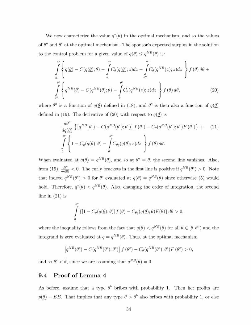
We now characterize the value q∗(θ) in the optimal mechanism, and so the values

of θa and θc at the optimal mechanism. The sponsor’s expected surplus in the solution

to the control problem for a given value of q(θ) ≤ qNB(θ) is:

θa∫θ

q(θ)− C(q(θ); θ)−θa∫θ

Cθ(q(θ); z)dz −θc∫

θa

Cθ(qNB(z); z)dz

f (θ) dθ +

θc∫θa

qNB(θ)− C(qNB(θ); θ)−θc∫θ

Cθ(qNB(z); z)dz

f (θ) dθ, (20)

where θa is a function of q(θ) defined in (18), and θc is then also a function of q(θ)

defined in (19). The derivative of (20) with respect to q(θ) is

dθc

dq(θ)

{[qNB(θc)− C(qNB(θc); θc)

]f (θc)− Cθ(qNB(θc); θc)F (θc)

}+ (21)

θa∫θ

1− Cq(q(θ); θ)−θa∫θ

Cθq(q(θ); z)dz

f (θ) dθ.

When evaluated at q(θ) = qNB(θ), and so at θa = θ, the second line vanishes. Also,

from (19), dθc

dq(θ)< 0. The curly brackets in the first line is positive if qNB(θc) > 0. Note

that indeed qNB(θc) > 0 for θc evaluated at q(θ) = qNB(θ) since otherwise (5) would

hold. Therefore, q∗(θ) < qNB(θ). Also, changing the order of integration, the second

line in (21) is

θa∫θ

{[1− Cq(q(θ); θ)] f (θ)− Cθq(q(θ); θ)F (θ)} dθ > 0,

where the inequality follows from the fact that q(θ) < qNB(θ) for all θ ∈ [θ, θa) and the

integrand is zero evaluated at q = qNB(θ). Thus, at the optimal mechanism[qNB(θc)− C(qNB(θc); θc)

]f (θc)− Cθ(qNB(θc); θc)F (θc) > 0,

and so θc < θ, since we are assuming that qNB(θ) = 0.

9.4 Proof of Lemma 4

As before, assume that a type θb bribes with probability 1. Then her profits are

p(θ) − EB. That implies that any type θ > θb also bribes with probability 1, or else

34

q(θ) = 0. Indeed, Π(θ) = Π(θb), since type θ can always imitate type θb and obtain

the same profits, p(θ)−EB. But if q(θ) > 0 and b(θ) > B, then θb would benefit from

deviating and imitating type θ, since her costs are lower. Thus, assume that for all

types θ ≥ θb either q(θ) = 0 or b(θ) = B. Define (p′, q′, b′) where (p′(θ), q′(θ), b′(θ)) =

(p(θ), q(θ), b(θ)) for all θ < θb, but (p′(θ), q′(θ), b′(θ)) = (p(θ) − EB, 0, B) for θ > θb.

Note that, conditional on truth-telling, the profits of all types are unchanged. Moreover,

the profits of any deviating type are still the same, and so (p′, q′, b′) is IC and IR. On

the other hand the payoff for the sponsor is larger, weakly so if the the measure of

types θ > θb with b(θ) = B is zero.

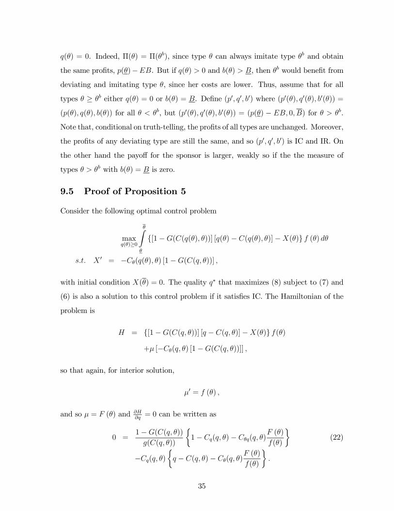
9.5 Proof of Proposition 5

Consider the following optimal control problem

maxq(θ)≥0

θ∫θ

{[1−G(C(q(θ), θ))] [q(θ)− C(q(θ), θ)]−X(θ)} f (θ) dθ

s.t. X ′ = −Cθ(q(θ), θ) [1−G(C(q, θ))] ,

with initial condition X(θ) = 0. The quality q∗ that maximizes (8) subject to (7) and

(6) is also a solution to this control problem if it satisfies IC. The Hamiltonian of the

problem is

H = {[1−G(C(q, θ))] [q − C(q, θ)]−X(θ)} f(θ)

+µ [−Cθ(q, θ) [1−G(C(q, θ))]] ,

so that again, for interior solution,

µ′ = f (θ) ,

and so µ = F (θ) and ∂H∂q

= 0 can be written as

0 =1−G(C(q, θ))

g(C(q, θ))

{1− Cq(q, θ)− Cθq(q, θ)

F (θ)

f(θ)

}(22)

−Cq(q, θ){q − C(q, θ)− Cθ(q, θ)

F (θ)

f(θ)

}.

35

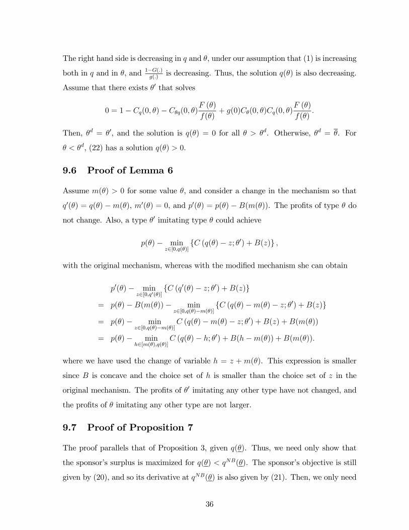
The right hand side is decreasing in q and θ, under our assumption that (1) is increasing

both in q and in θ, and 1−G(.)g(.)

is decreasing. Thus, the solution q(θ) is also decreasing.

Assume that there exists θ′ that solves

0 = 1− Cq(0, θ)− Cθq(0, θ)F (θ)

f(θ)+ g(0)Cθ(0, θ)Cq(0, θ)

F (θ)

f(θ).

Then, θd = θ′, and the solution is q(θ) = 0 for all θ > θd. Otherwise, θd = θ. For

θ < θd, (22) has a solution q(θ) > 0.

9.6 Proof of Lemma 6

Assume m(θ) > 0 for some value θ, and consider a change in the mechanism so that

q′(θ) = q(θ)−m(θ), m′(θ) = 0, and p′(θ) = p(θ)− B(m(θ)). The profits of type θ do

not change. Also, a type θ′ imitating type θ could achieve

p(θ)− minz∈[0,q(θ)]

{C (q(θ)− z; θ′) +B(z)} ,

with the original mechanism, whereas with the modified mechanism she can obtain

p′(θ)− minz∈[0,q′(θ)]

{C (q′(θ)− z; θ′) +B(z)}

= p(θ)−B(m(θ))− minz∈[0,q(θ)−m(θ)]

{C (q(θ)−m(θ)− z; θ′) +B(z)}

= p(θ)− minz∈[0,q(θ)−m(θ)]

C (q(θ)−m(θ)− z; θ′) +B(z) +B(m(θ))

= p(θ)− minh∈[m(θ),q(θ)]

C (q(θ)− h; θ′) +B(h−m(θ)) +B(m(θ)).

where we have used the change of variable h = z + m(θ). This expression is smaller

since B is concave and the choice set of h is smaller than the choice set of z in the

original mechanism. The profits of θ′ imitating any other type have not changed, and

the profits of θ imitating any other type are not larger.

9.7 Proof of Proposition 7

The proof parallels that of Proposition 3, given q(θ). Thus, we need only show that

the sponsor’s surplus is maximized for q(θ) < qNB(θ). The sponsor’s objective is still

given by (20), and so its derivative at qNB(θ) is also given by (21). Then, we only need

36

show that dθc

dq(θ)< 0. Totally differentiatin the equivalent now to (19),

B(q(θ))− C(q(θ); θ)−θa∫θ

Cθ(q(θ); z)dz −θc∫

θa

Cθ(qNB(z); z)dz = 0,

we have

dθc

dq(θ)=

B′(q(θ))− Cq(q(θ); θ)−θa∫θ

Cθq(q(θ); z)dz

Cθ(qNB(θc); θc)< 0,

where the inequality follows from A2 and the fact that Cθq(q; θ) > 0.

37