producer participation in price pooling cooperatives to...
TRANSCRIPT
University of Arkansas
[email protected] $ (479) 575-7646
An Agricultural Law Research Article
Producer Participation in Price Pooling Cooperatives to Smooth
Income Variability: Evidence from California
by Devry S. Boughner and Daniel A. Sumner
Originally published in SAN JOAQUIN AGRICULTURAL LAW REVIEW 10 SAN JOAQUIN AGRIC. L. REV. 27 (2000)
www.NationalAgLawCenter.org
PRODUCER PARTICIPATION IN PRICE POOLING COOPERATIVES
TO SMOOTH INCOME VARIABILITY: EVIDENCE FROM
CALIFORNIA Devry S. Boughner and
Daniel A. Sumner*
ABSTRACT
Agricultural producers face price variability within a season and across years. Such price variability induces some producers to engage in the joint marketing of their product through price pooling organizations, such as marketing cooperatives. This article examines factors influencing producer participation in pooling organizations. An econometric study assesses the significance of variables in determining the percentage of price pooling that occurs in forty-four major agricultural industries in California. Results show that product differentiation, defined grade standards, product storability, and concentration of production are the factors that contribute most to enrollment in price pooling organizations.
I. BACKGROUND ON PRICE POOLING
Fann producers face price variability within the season and across years.! Prices received by farmers depend on a great number of con
* Devry S. Boughner is an Economist with The World Bank. Daniel A. Sumner, Ph.D. is the Frank H. Buck, lr. Professor of the Department of Agricultural and Resource Economics, University of California, Davis, and Director of the University of California Agricultural Issues Center. This study was initiated when Boughner was a research assistant at the University of California, Davis. The authors would like to convey appreciation to the following people for their assistance: Hoy F. Carman, Colin A. Carter, Leon Garoyan, lames Haskell, Andrew lermolowicz, Mahlon Lang, Richard Sexton, Norbert Wilson, and Christopher A. Wolf.
1 NICHOLAS 1. POWERS & RICHARD G. HEIFNER. U.S. DEP'T OF AGRIc.. FEDERAL GRADE STANDARDS FOR FREsH PRODUCE: LINKAGES TO PESTICIDE USE, 4 (Agric. Info. Bull. No. 675, Aug. 1993); FEDERAL MKT. NEWS SERV.. U.S. DEP'T OF AGRIC., Los
27
28 San Joaquin Agricultural Law Review [Vol. 10:27
trollable and uncontrollable variables (for example, weather, pests, disease, input price variation in other regions, output, demand variation, and government regulations, to name a few).
Farmers attempt to reduce income variability of returns in many ways. They spray to ward off pests, they enroll in government support programs, and they purchase insurance. Price pooling is one additional way to dampen the impact of market price fluctuations.2
Price pooling entails joint marketing by a group of producers (across industries and over time), each receiving a price averaged from the sale of the product in an attempt to smooth returns over time. The joint marketing can be based upon a single specific commodity or upon multiple commodities. Any number of pools can be formed by a pooling organization differentiated on the basis of variety, quality, season, type of product, or other characteristics.
Price pooling goes back to before 1920 as a method of spreading market risks among many producers.3 California agriculture was aggressive in making a success of pooling through cooperative marketing with oranges as early as the 1890s.4 The cotton industry was an early example of market pools. Price pooling was viewed as a means of transferring ownership of a commodity to a marketing cooperative in exchange for an average return, with progress payments made during the season.5
We may define two types of pools: the pure pool or seasonal pool, and what we call the mixed pool. Based on our survey discussed below, some marketing cooperatives only operate pure pools; others operate mixed pools, and some operate both pure and mixed pools, giving the producer a choice. In a pure pool, 100% of the product is pooled; the producer relinquishes all management control and all marketing decisions are handled by a central staff.6 The producer receives returns from pooling over time with advance payments and equalization payments made at the designated close of the pooP Equalization
ANGELES FREsH FRUIT AND VEGETABLE WHOLESALE MARKET PRICES 1995, 7-77. 2 T.M. HAMMONDS, OREGON ST. D., COOPERATIVE MARKET POOLING, 1 (Circular of
Info. 652, Nov. 1976). 3 AARON SAPIRO, AMERICAN FARM BUREAU FED'N, CO-OPERATIVE MARKETING
(1920). 4 AARON SAPIRO, ONTARIO DEP'T OF AGRIC., ADDRESSES ON CO-OPERATIVE MARKET
ING, 5 (1922). 5 [d.
6 HAMMONDS, supra note 2, at 1. 7 [d. at 2.
29 2000] Price Pooling Cooperatives
payments adjust for product quality and variety differences.8 In a mixed pool, the farmer chooses the amount pooled and has other options such as a delayed pricing program or hedging incentives.9 In this case, producers have increased managerial opportunities and they retain some control over the time or price at which the product will be sold. to One may also define forms of price pooling: mandatory and voluntary. Because we focus on grower choice, this study examines only voluntary participation in price pooling organizations. Thus, mandatory milk price pooling is not a subject of study here. II
There have been only a few studies on the conditions conducive to price pooling (generally through marketing cooperatives); this is the first attempt to examine participation in price pooling econometrically. Previous studies have been descriptions,12 surveys,13 or opinions rather than econometric analyses that relate to a group of agricultural commodities.
Hammonds explains the fundamentals of price pooling and examines in detail the strategies of five cooperative market pools positioned around the United States.14 His work was based on personal interview and record inspection of the selected marketing cooperatives. IS Sexton examines three reasons for joint action by farmers: creation of market power, exploitation of size economies, and risk pooling. 16 Sexton notes that most marketing cooperatives operate with some type of price pooling arrangements which assist in performing functions such as risk spreading and market insurance.17
Garoyan reviews the importance of operating a properly structured pool.I8 He focuses on the issue of incentives by quality and type
8Id. 9 Id. at 2-3. 10 Id. II But see, e.g., Daniel A. Sumner & Tom Cox, FAIR Dairy Policy, 16 CONTEMPO
RARY EcON. POL'y., Feb. 1998, 59-60. 12 See DAVID K. SMITH & HENRY N. WALLACE, U.S. DEP'T OF AGRIc., COOPERA
TIVES IN CALIFORNIA AGRICULTURE, (Agric. Coop. Servo Res. Rep. 87: Feb. 1990). 13 See CAROLE BARNES ET AL., U.e. DAVIS, How CALIFORNIANS SEE COOPERATIVES,
1-4 (1995). 14 HAMMONDS, supra note 2. I~ Id.
16 RICHARD 1. SEXTON, u.e. DAVIS, THE EcONOMIC ROLE OF COOPERATIVES IN MARKET-ORIENTED ECONOMICS (1995).
17 Id. at 5. 18 LEON GAROYAN, u.e. DAVIS, CALIFORNIA'S CONTRIBUTIONS TO COOPERATION
(1989).
30 San Joaquin Agricultural Law Review [Vol. 10:27
within overall pOOIS.19 Garoyan notes that pooling could be a crucial factor in determining the price of a commodity if the pooling organi~
zation controls a relatively large share of the total market.20 Sosnick focuses on the marketing of fresh avocados by Calavo Growers of California,21 a cooperative group that now handles about forty-eight percent of the California avocado market.22 Sosnick addresses pooling alternatives that Calavo offers its producers.23 He examines product grading and creating member equity in specific pools.24 The study provides insight on how detailed the pooling process can become with a heterogeneous product such as avocados.
None of these studies attempts to explain voluntary participation in pooling organizations econometrically. In the next section, we present the conceptual and empirical models that are used to explain the relevance of specific variables in motivating the practice of price pooling.
II. CONCEPTUAL MODEL
For a profit maximizing farmer to participate, benefits of pooling must outweigh direct costs and be greater than benefits from other methods of price stabilization. Prevalence of pooling in an industry therefore depends on specific characteristics of the market for the product, historical factors associated with price pooling, and sociological factors. For example, the reputation of major cooperatives in an industry can influence pooling. Further, producers who grow a single crop may use price pooling rather than diversification to smooth farm returns. Pooling would be less likely in industries where some producers would seem to be regularly subsidizing other producers.
As noted above, growers have a broad array of options regarding decisions to limit or control price variability. This study focuses solely upon measurable factors that affect the demand for price pooling by individual producers. The independent variables selected are based on conditions of the market for a grower's commodity and on the physical characteristics of the commodity. It is necessary to stress that we
19 [d. at 11-12. 2Il [d. at 12. 21 Stephen H. Sosnick, Optimal Cooperative Pools for California Avocados, 35 Hil
gardia: J. Agric. Sci. (published by the Cal. Agric. Experiment Station 47, 47-48 (1963)).
22 E-mail correspondence from Mark Nolan, Calavo Growers of California (Dec. 22, 1999) (on file with the San Joaquin Agricultural Law Review).
23 [d. at 47-48. 24 [d.
31 2000] Price Pooling Cooperatives
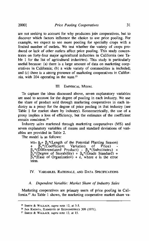
are not seeking to account for why producers join cooperatives, but to discover which factors influence the choice to use price pooling. For example, we expect to see more pooling for specialty crops with a limited number of outlets. We test whether the variety of crops produced or lack of other outlets affect price pooling. This study concentrates on forty-four major agricultural industries in California (see Table 1 for the list of agricultural industries). This study is particularly useful because: (a) there is a large amount of data on marketing cooperatives in California; (b) a wide variety of commodities is included; and (c) there is a strong presence of marketing cooperatives in California, with 204 operating in the state.25
III. EMPIRICAL MODEL
To capture the ideas discussed above, seven explanatory variables are used to account for the degree of pooling in each industry. We use the share of product sold through marketing cooperatives in each industry as a proxy for the degree of price pooling in that industry (see Table 1 for market share by industry). Econometrically, the use of a proxy implies a loss of efficiency, but the estimates of the coefficient remain consistent.26
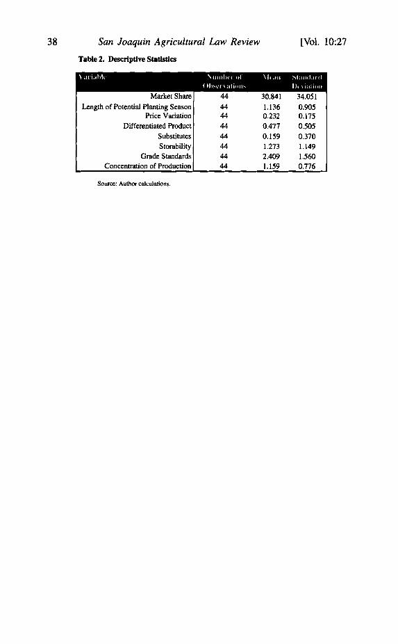
Industry sales marketed through marketing cooperatives (MS) and seven explanatory variables of means and standard deviations of variables are provided in Table 2.
The model is as follows:
MS= ~o+ ~ *(Length of the Potential Planting Season) + ~z*(Coefficient Variation of Price) 3*(Dlfferentiated Product) - ~A*(Substitutes) + s*(Degree of Storability) + ~6*(lirade Standard) + 7*(Ease of Organization) + e, where e is the error ~
term.
IV. VARlABLES, RATIONALE, AND DATA SPECIFICATIONS
A. Dependent Variable: Market Share of Industry Sales
Marketing cooperatives are primary users of price pooling in California.27 As Table 1 shows, the marketing cooperative market share va
2' SMITH & WALLACE, supra note 12, at 3-5. 26 JAN KMEN'rA, ELEMENTS OF EcONOMETRICS 309 (1971). 27 SMITH & WALLACE, supra note 12, at 15.
32 San Joaquin Agricultural Low Review [Vol. 10:27
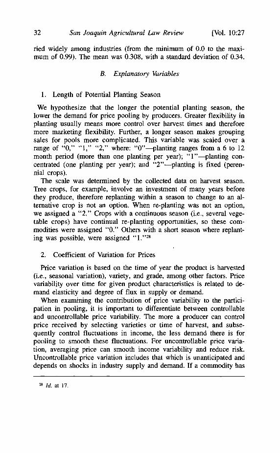
ried widely among industries (from the minimum of 0.0 to the maximum of 0.99). The mean was 0.308, with a standard deviation of 0.34.
B. Explanatory Variables
1. Length of Potential Planting Season
We hypothesize that the longer the potential planting season, the lower the demand for price pooling by producers. Greater flexibility in planting usually means more control over harvest times and therefore more marketing flexibility. Further, a longer season makes grouping sales for pools more complicated. This variable was scaled over a range of "0," "1," "2," where: "0"-planting ranges from a 6 to 12 month period (more than one planting per year); "1"-planting concentrated (one planting per year); and "2"-planting is fixed (perennial crops).
The scale was determined by the collected data on harvest season. Tree crops, for example, involve an investment of many years before they produce, therefore replanting within a season to change to an alternative crop is not an option. When re-planting was not an option, we assigned a "2." Crops with a continuous season (Le., several vegetable crops) have continual re-planting opportunities, so these commodities were assigned "0." Others with a short season where replanting was possible, were assigned "1. "28
2. Coefficient of Variation for Prices
Price variation is based on the time of year the product is harvested (Le., seasonal variation), variety, and grade, among other factors. Price variability over time for given product characteristics is related to demand elasticity and degree of flux in supply or demand.
When examining the contribution of price variability to the participation in pooling, it is important to differentiate between controllable and uncontrollable price variability. The more a producer can control price received by selecting varieties or time of harvest, and subsequently control fluctuations in income, the less demand there is for pooling to smooth these fluctuations. For uncontrollable price variation, averaging price can smooth income variability and reduce risk. Uncontrollable price variation includes that which is unanticipated and depends on shocks in industry supply and demand. If a commodity has
28 ld. at 17.
33 2000] Price Pooling Cooperatives
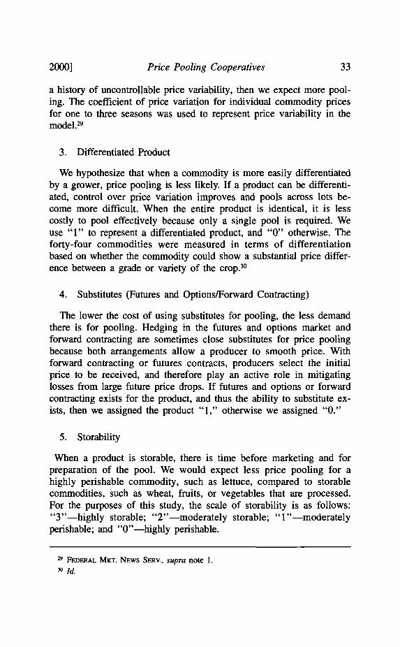
a history of uncontrollable price variability, then we expect more pooling. The coefficient of price variation for individual commodity prices for one to three seasons was used to represent price variability in the model.29
3. Differentiated Product
We hypothesize that when a commodity is more easily differentiated by a grower, price pooling is less likely. If a product can be differentiated, control over price variation improves and pools across lots become more difficult. When the entire product is identical, it is less costly to pool effectively because only a single pool is required. We use "1" to represent a differentiated product, and "0" otherwise. The forty-four commodities were measured in terms of differentiation based on whether the commodity could show a substantial price difference between a grade or variety of the crop.30
4. Substitutes (Futures and Options/Forward Contracting)
The lower the cost of using substitutes for pooling, the less demand there is for pooling. Hedging in the futures and options market and forward contracting are sometimes close substitutes for price pooling because both arrangements allow a producer to smooth price. With forward contracting or futures contracts, producers select the initial price to be received, and therefore play an active role in mitigating losses from large future price drops. If futures and options or forward contracting exists for the product, and thus the ability to substitute exists, then we assigned the product "1," otherwise we assigned "0."
5. Storability
When a product is storable, there is time before marketing and for preparation of the pool. We would expect less price pooling for a highly perishable commodity, such as lettuce, compared to storable commodities, such as wheat, fruits, or vegetables that are processed. For the purposes of this study, the scale of storability is as follows: "3"-highly storable; "2"-moderately storable; "1"-moderately perishable; and "0"-highly perishable.
29 FEDERAL MKT. NEWS SERV.• supra note 1. 30 [d.
34 San Joaquin Agricultural Law Review [Vol. 10:27
6. Accepted Quality/Grade Standards Across Industry
When various grades of a commodity command different prices, separate pools by grade may be used.31 If some farmers supply higher quality products that are pooled with other farmers' lower quality products, there is loss of benefits to quality for that individual farmer. This creates lower incentive to produce better quality. Loss of incentive for quality may be mitigated by specifying more tightly the quality or grade standards required for each pool.32 Therefore, we hypothesize that industries with established and accepted grade standards are more apt to price pool.
The scale used in the study is as follows: "4"-mandatory use of federal or industry grade standards or low cost grading; "3"-most frequent use of federal or industry grade standards; "2"-frequent use of federal or industry grade standards; "1"-less frequent use of federal or industry grade standards; and "0"-infrequent or no use of federal or industry grade standards.33
7. Concentration of Production (Ease of Organization)
The more centrally located the production for a specific crop, the easier it is to organize a price pooling cooperative for that crop. If a group of producers are concentrated within a small radius, a personal relationship between growers is more likely to develop. Geographic concentration also means more weather-based supply variability. We hypothesize that agricultural commodity industries with a high concentration of production, meaning that the crop is grown in neighboring counties, practice more pooling. Concentration of crop was based on the 1995 Agricultural Commissioners' Data.34 The scale is as follows: "2"-strong concentration of production; "1"-medium concentration of production; "0"-scattered or no concentration of production.
V. ESTIMATED MODELS, RESULTS, AND DISCUSSION
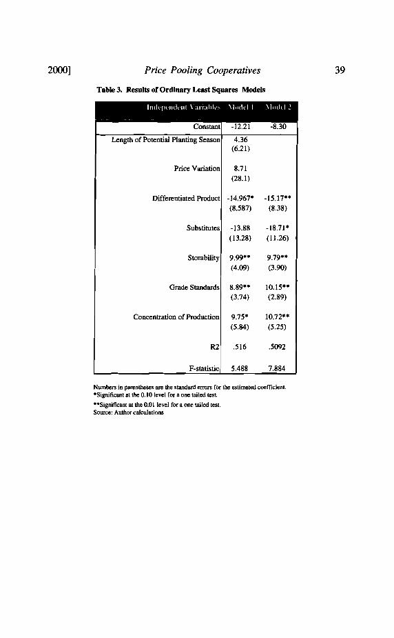
Estimation results for two Ordinary Least Squares (OLS) models are presented in Table 3. The dependent variable for each model is the share of industry sales marketed through marketing cooperatives (see Table 1 for market shares). We estimate by OLS to allow a more di
31 HAMMONDS. supra note 2, at 2. 32 GAROYAN, supra note 18, at 11. 33 POWERS & HEIFNER, supra note I, at 15-16. 34 CALIFORNIA AORIC. STAT. SERV., CAL. DEP'T OF FOOD AND AGRIc., 1995 AGRICUL
TURAL COMMISSIONERS' DATA, (1996).
35 2000] Price Pooling Cooperatives
rect interpretation of coefficients while recognizing that most shares are in the middle range of the data and that parameter estimates remain consistent. Maximum likelihood methods such as a probit or logit model are less robust to functional fonn specification errors.
All seven independent variables are included in Modell. They explain just over half of the variation in share across the forty-four agricultural industries because OLS predicted values are not constrained, and predicted values for five industries fell below zero.
Accepted Grade Standards and the Degree of Storability variables were strongly significant at the 0.05 level. We hypothesized that grading standards make it easier to operate an effective pooling organization. We also hypothesized that the higher cost of storage would have a positive effect on the demand for price pooling. We failed to reject the hypotheses and both effects are consistent with our model.
Differentiation was found to be significant at the 0.05 level. We hypothesized that if a product could be differentiated, then it would be more costly and less effective to operate a pool. The results fail to reject this hypothesis. Concentration or Ease of Organization has a positive effect on price pooling at about the 0.10 level, which is also as expected.
The coefficients for the variables Length of Potential Planting Season and Price Variation were both much smaller than their standard errors. Both variables faced measurement problems. The measurements for price variation were poor: (1) prices were collected for only one season for each industry; (2) no seasonal trend deviation was accounted for; and (3) we were not able to separate controllable verses uncontrollable variations. Thus while we used the best proxy available for this variable, we were not surprised when this proxy variable failed to capture the expected effect.
Existence of Substitutes was expected to have a negative effect on price pooling. Existence of futures and options or forward contracting does indeed cause a decrease in demand for price pooling. Such substitutes attract producers away from price pooling because producers find alternative methods to smoothing returns over time. A better variable for the degree of uncontrollable variability may be needed to make this variable more significant (which may also be jointly determined with pooling). In fact, some cooperatives even require their members to hedge on a commodity exchange.
As a test of robustness and stability of coefficients, we examined the model excluding both the Price Variation and the Length of Potential Planting Season variables in Model 2. The R2 fell slightly, but the
36 San Joaquin Agricultural Law Review [Vol. 10:27
F-statistics rose. In this model, the estimated coefficient for the Differentiation variable increased while the standard error decreased.
A notable difference can be seen in the level of significance for Accepted Grade Standards. The estimated coefficient increased from 8.89 to 10.15, while the standard error decreased from 3.74 to 2.89. Concentration is now more significant at the 0.05 level with the exclusion of both variables and the Substitutes variable now reaches a 0.05 significance level for the one tail test.
CONCLUDING REMARKS: LIMITATIONS AND CRITICAL FINDINGS
This research is the first to empirically measure how variables related to income smoothing relate to participation in price pooling in cooperatives in California. The data support our main hypotheses. Pooling responds to product and industry characteristics and to the existence of substitute institutions. There were limitations on this study. The share of price pooling was measured by market share of marketing cooperatives; a detailed and specialized survey would be required for better data. Better data on past price variation and the source of that variation by specific grade and other marketing characteristics would serve as a better proxy of uncontrollable price variation for each commodity. A more complete model of the full set of farm decisions related to pooling would be helpful to place pooling in the proper context. More characteristics of growers within the specified agricultural industries would also be useful (for example, the size of farms across industries).
Overall, this study presents useful results that show price pooling is significantly related to: (1) product differentiation; (2) defined grade standards; (3) storability; and (4) concentration of production, and availability of substitute institutions. Price pooling is less significantly related to availability of substitute institutions.35
35 HAMMONDS, supra note 2, at 4-11.
37 2000] Price Pooling Cooperatives
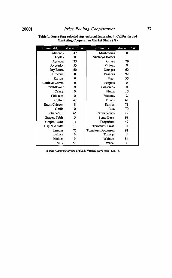
Table 1. Forty-four selected Agricultural Industries in California and Marketing Cooperative Market Share (%)
( ollll11odit, \tll kl'1 Share ( ollllllodit, \tll kLl Sh.lIl'
Almonds Apples
Apricots Avocados Dry Beans
Broccoli
Carrots Cattle & Calves
Cauliflower Celery
Chickens Cotton
Eggs. Chicken Garlic
Grapefruit Grapes. Table Grapes. Wine
Hay & Alfalfa
Lemons Lettuce Melons
Milk
47 o 75 53 60 o o o o o o 47 8 o 65 5 11 11 75 6 o 58
Mushrooms NurserylFlowers
Olives Onions
Oranges Peaches
Pears
Peppers Pistachios
Plums Potatoes
Prunes
Raisins Rice
Strawberries Sugar Beets Tangerines
Tomatoes. Fresh Tomatoes. Processed
Turkeys Walnuts
Wheat
o I
70 o 60 92 50 o o 10 2
61 78 70 22 99 42 o
91 o
84 4
Source: Author survey and Smith & Wallace. supra nole 12. at 13.
-----
38 San Joaquin Agricultural Law Review [Vol. 10:27
Table 2. Descriptive Statistics
\ aria"'"
Market Share
Length of Potential Planting Season Price Variation
Differentiated Product
Substitutes Storability
Grade Standards Concentration of Production
Source: Author calculations.
"lim",,!" "I ()h"'\"I"' atioll'"
44
44 44 44 44 44 44 44
\kall
30.841
1.136 0.232
0.477
0.159
1.273 2.409 1.159
Sl","lard I k\ iatioll
34.051
0.905 0.175
0.505
0.370
1.149
1.560 0.776
39 2000] Price Pooling Cooperatives
Table 3. Results of Ordinary Least Squares Models
IrUkpl'lukll1 \ aridhll" \J"dd I \I,,(h 12
Constant
Length of Potential Planting Season
-12.21
4.36 (6.21)
-8.30
Price Variation 8.71 (28.1)
Differentiated Product -14.967* (8.587)
-15.17** (8.38)
Substitutes -13.88 (13.28)
-18.71* (11.26)
Storability 9.99** (4.09)
9.79** (3.90)
Grade Standards 8.89** (3.74)
10.15** (2.89)
Concentration of Production 9.75* (5.84)
10.n** (5.25)
R2 .516 .5092
F-statistic 5.488 7.884
Numbers in parentheses are the standard errors for the estimated coefficient. ·Significant at the 0.10 level for a one tailed test.
··Significant at the 0.01 level for a one tailed test. Source: Author calculations