production quota in multiproduct pacific fisheries*
TRANSCRIPT
ANAL OF ENVIRONMENTAL ECONOMICS AND MANAGEMENT 21, 109-126 (1991)
Production Quota in Multiproduct Pacific Fisheries*
DALE SQUIRES
National Marine Fisheries Seruice, Southwest Fisheries Center, P.O. Box 271, La Jolla, California 92038
A N D
JAMES KIRKLEY
College of William and Mary, School of Business Administration and School of Marine Science, Gloucester Point, Virginia
Received May 16, 1990; revised December 14, 1990
Assessing the individual firm’s technology and costs in a multispecies fishery allows design of a more effective output quota prior to regulation by anticipating and controlling for the firm’s regulation-induced responses. An empirical study of a Pacific coast trawl fishery indicates that the firm’s flexibility of product decision is tightly constrained by its technology and cost structure. Hence, as the resource stock for the regulated species, sablefish, deteriorates and the trip quota progressively tightens, the firm cannot sufficiently reorganize its product bundle to preclude increasingly large sablefish disposal. This defeats the purpose of the production quota. 0 1991 Academic Press, Inc.
1. INTRODUCTION
Quotas on individual outputs are often used to regulate production flows of individual firms in multispecies (multiproduct) fisheries. In response to a quota, firms attempt to reorganize the mix and volume of the other species (outputs). If only limited changes are possible, production in excess of quota may be discarded, creating technically inefficient production and unnecessary fish mortality. Alterna- tively, when the mix and volume of other species produced are easily changed, these resource stocks may be threatened by excess production. Over a longer time period, output quotas can also induce changes in the quantities of quasi-fixed factors and further reduce production.
The competitive multispecies firm’s regulation-induced reorganizations of its optimum output bundle depend upon the firm’s technology and cost structure. Hence, tailoring quota design to technology and costs anticipates many quota- induced economic responses and allows design of a more effective quota.
Empirical studies of output quantity controls for the competitive multiproduct firm in a certain and static environment have usually been retrospective, analyzing
*The authors thank the editor, two anonymous referees, Ralph Brown and Dick Young-two commercial fishermen, and Harry Campbell, Jim Golden, Paul Heikkila, Tom Hertel, Wes Silverthorne, and Geoff Waugh for helpful discussions. Pete Leipzig of the Eureka Fishermen’s Association kindly identified vessels with high-speed winches. The conclusions are not necessarily those of the National Marine Fisheries Service or the Virginia Institute of Marine Science. The authors remain responsible for any remaining errors. Squires is grateful to the Department of Economics, University of Queens- land, where this work was completed while he was a Visiting Lecturer there.
109 0095-0696/91 $3.00
Copyright 0 1YY1 by Academic Press. Inc. All rights of reproduction i n any form reserved.
110 SQUIRES AND KIRKLEY
comparative statics in a post-regulatory regime [13, 151. Kirkley and Strand [7] and Squires [21] considered some of these issues when all outputs were unregulated and hence decision variables, but they did not consider the issue of the competitive firm’s economic response to output regulation, and did not explicitly consider quotas.
This paper addresses the design of a command-and-control output quota which is consistent with the currently unregulated, revenue-maximizing multispecies firm’s technology and cost structure when all outputs are decision variables. The emphasis is upon the firm’s initial response to quota. We assess the competitive firm’s reorganization of its optimum product bundle and changes in its quasi-fixed factor in response to a binding output quota. We examine the firm’s short-run response to the output quota over a time period sufficiently short to assume that the abundance of the resource stock remains effectively constant and the capital stock does not adjust to its optimum full static equilibrium level; a longer-run analysis requires a more detailed bioeconomic model.
A multispecies trawl fishery off the Eureka, California area offers a case study.’ A command-and-control quota on the quantity of sablefish landed at port for each vessel’s fishing trip regulates production flows in the deep-water fishery of the continental slope for sablefish. The goals are to prevent overproduction, conserve the resource stock, maintain a year-round fishery, and enhance economic rent. The paper finds that limited flexibility to reorganize the mix and volume of outputs in response to the sablefish quota induces discards of excess production and pre- cludes effective use of a command-and-control quota as a management tool.
Section 2 discusses the approach and methodology. Section 3 relates output quotas to the firm’s technology and cost structure; additional detail is placed in the Appendix. Section 4 discusses the data, the model, and the empirical results. The final section contains concluding remarks.
2. THE APPROACH AND METHODOLOGY
The analysis assumes that unregulated firms maximize profit in two stages. In the first stage, a fishing trip, vessel operators choose their revenue-maximizing output bundle given fixed inputs, weather and resource abundance constraints, and relative product prices. Inputs on the vessel are largely fixed during a trip due to the short production period of 1 to 5 days and boats are away at sea where input levels Cannot be readily changed. In this first stage, revenue-maximizing vessels are in partial equilibrium, Le., firms maximize revenues conditional upon the quasi- fixed factors.
The input bundle can be specified as a single, composite input, since vessel size or capital stock is fixed at the trip level and largely determines the level of other inputs. The services of some inputs (particularly fuel) may vary with time at sea during an individual fishing trip, but the time at sea varies only slightly and the variation is not systematic. Revenue maximization subject to a single quasi-fixed input appears to be a reasonable assumption for a multispecies fishing firm making
‘The region includes Eureka and Crescent City in California and Brookings in Oregon. Otter trawlers drag a net, then haul in the net, dump and sort the catch on deck, and store it below.
FISHERIES PRODUCTION QUOTA 111
output decisions over such a short production period [6, 7].2 This composite input is called effort, following the fisheries literature.
In the second stage of production, over a time period varying roughly between 3 to 14 months, fishing firms adjust the level of effort to minimize their production costs by selecting the optimal vessel size or capital stock. This paper’s focus is upon the first stage of production.
The revenue function provides a duality-based approach to examine the underly- ing short-run production technology when, in the first stage of production, the firm is free to choose its revenue-maximizing output bundle with the composite input quasi-fixed. The revenue function provides the maximum revenue for the given level of the composite input, product prices, state of technological knowledge, and technical constraints to production. The revenue function was developed by McFadden [14], and the specialized form with a single composite input was introduced by Diewert [4]. The revenue function for a single, composite input Z is defined by R[P; Z ] = max,(P’Y: Y E L(Z)), where Y is an M X 1 vector of endogenous products with a vector of competitive, exogenous prices P ; is the transpose operator; and L(Z) represents the firm’s output possibilities set when all factors are fixed but products are decision variables. Regularity conditions are given by McFadden [14] and Sakai [19].
A nonhomothetic generalized Leontief revenue function models the revenue- maximizing vessel-level production process for an unregulated fishing trip [6, 71,
R [ P ; Z ] = ~ A l , ( P l ~ ) ” z z + c A , P , Z z 1 1 1
where R(P ; Z ) is the revenue function, Pi is the product price of species i , 2 is the composite input, D, is the k th of two home port dummy variables for Brookings and Crescent City, and E, is the Ith of three quarterly dummy variables for winter, spring, and fall. The base case accounts for Eureka in the summer. The area dummy variables account for spatial variations in access to fish stocks, species abundance, and port effects on prices. The quarterly dummy variables G account for intertemporal variations in the technological constraints of weather and re- source abundance.
Hotelling’s Lemma gives input-compensated supply functions for unregulated production Y(P; Z> 1141:
6R[ P ; Z]/6P, = Y,( P ; Z ) = A,,Z + A , Z 2 + BIkDkZ k
Symmetry is imposed by A,, = A , , , i not equal to j . Zero homogeneity in prices follows from the Generalized Leontief form.
*Formally, Leontief input separability is assumed, where input quantities move in fixed proportions over time.
112 SQUIRES AND KIRKLEY
The input-compensated supply functions for unregulated production, Eq. (21, were estimated for vessels of at least 75 gross registered tons (GRT) which landed at least 1,000 pounds of sablefish in 1984. Catch and landings were equal and there was no quota-induced disposal at sea because 1984 was the last unregulated year (without quota). We considered only vessels with a high-speed winch allowing them to exploit a deep-water continental slope fishery concentrated on Dover sole, thornyheads, and sablefish. This fishery is centered in the area studied. Several other species were also harvested to utilize excess hold capacity and enjoy product diversity. Six species or outputs were specified: Dover sole, thornyheads, sablefish, other flatfish, other rockfish, and a residual, all others. There were 444 observa- tions (fishing trips) on 14 vessels, with an unequal number of observations for each vessel.
3. OUTPUT QUOTAS AND THE STRUCTURE OF COST AND TECHNOLOGY
Effective quotas for regulating multiproduct firms require information on the structure of technology and costs. In this section, we discuss technical and economic characteristics specific to multiproduct production with significant impli- cations for imposing output quotas on multiproduct firms.
3.1. Technology Tests
The form of the production technology can be assessed by likelihood ratio tests of various hypotheses. The final form of the technology has important ramifica- tions for regulation [6, 7, 211.
Input-output separability. Separability between inputs and the M outputs im- plies no specific interaction between any one output and any one input [9]. The technology can then be specified as a single composite output and a single composite input. Only the levels of the catch and effort require regulation, and regulation of the species (input) mix does not adversely affect the optimal factor (product) combinations 17, 211. If the technology is separable between outputs and the fixed input, the Generalized Leontief revenue function with one input is separable in P and Z , i.e., R [ P ; Z ] = R[P]Z [7]. The marginal rates of transfor- mation of all output pairs are independent of factor intensities The economet- ric restriction is Ai = 0, i = 1,. . . , M.
A production process joint in inputs requires all inputs to produce all outputs. When production is nonjoint in inputs, separate production functions exist for each output or set of outputs. Hence, each production process can be separately regulated without affecting production of the other processes because there are no technological or cost tradeoffs between the output of one process and that of another [7, 211. Nonjointness in inputs over all species implies that the Generalized Leontief revenue function with a single input is written [7]: R[ P ; Z ] = Ei Ri[ P ; Z ] . Producers maximize outputs; Le., the supply of each species
Jointness-in-inputs.
'Since the partition is limited to two subsets, weak and strong separability are equivalent restric- tions.
FISHERIES PRODUCTION QUOTA 113
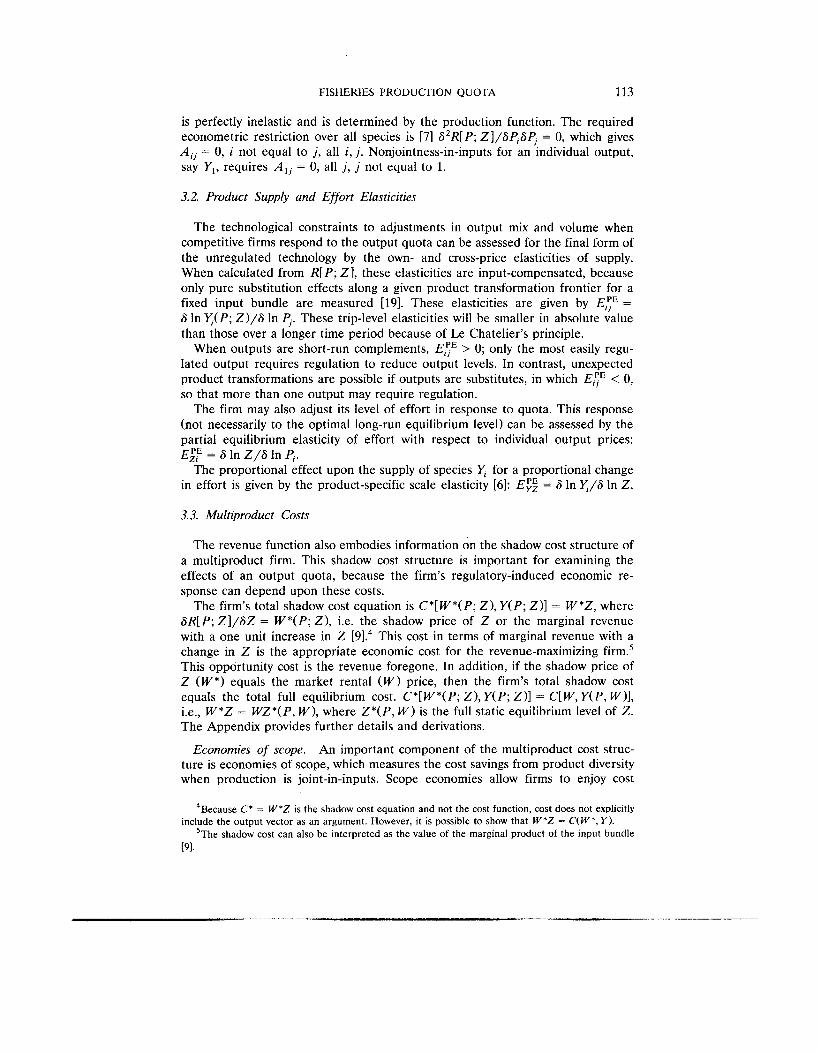
is perfectly inelastic and is determined by the production function. The required econometric restriction over all species is [7] 6*R[P; Z]/6Pj6P, = 0, which gives A j j = 0, i not equal to j , all i , j . Nonjointness-in-inputs for an individual output, say Y,, requires A , , = 0, all j , j not equal to 1.
3.2. Product Supply and Effort Elasticities
The technological constraints to adjustments in output mix and volume when competitive firms respond to the output quota can be assessed for the final form of the unregulated technology by the own- and cross-price elasticities of supply. When calculated from R[ P; Z ] , these elasticities are input-compensated, because only pure substitution effects along a given product transformation frontier for a fixed input bundle are measured [191. These elasticities are given by E,:E = 6 In x ( P ; Z ) / 6 In P,. These trip-level elasticities will be smaller in absolute value than those over a longer time period because of Le Chatelier's principle.
When outputs are short-run complements, E:" > 0; only the most easily regu- lated output requires regulation to reduce output levels. In contrast, unexpected product transformations are possible if outputs are substitutes, in which E:" < 0, so that more than one output may require regulation.
The firm may also adjust its level of effort in response to quota. This response (not necessarily to the optimal long-run equilibrium level) can be assessed by the partial equilibrium elasticity of effort with respect to individual output prices: El: = 6 In Z/6 In P,.
for a proportional change in effort is given by the product-specific scale elasticity [6]: E;: = 6 In x / 6 In Z.
The proportional effect upon the supply of species
3.3. Multiproduct Costs
The revenue function also embodies information on the shadow cost structure of a multiproduct firm. This shadow cost structure is important for examining the effects of an output quota, because the firm's regulatory-induced economic re- sponse can depend upon these costs.
The firm's total shadow cost equation is C*[W*(P; Z ) , Y ( P ; Z ) ] = W*Z, where 6R[P; Z ] / 6 Z = W*(P; Z ) , i.e. the shadow price of Z or the marginal revenue with a one unit increase in Z [9].4 This cost in terms of marginal revenue with a change in Z is the appropriate economic cost for the revenue-maximizing firm.5 This opportunity cost is the revenue foregone. In addition, if the shadow price of Z ( W * ) equals the market rental ( W ) price, then the firm's total shadow cost equals the total full equilibrium cost. C*[W*(P; Z ) , Y ( P ; Z ) ] = C[W, Y ( P , W)], i.e., W*Z = WZ*(P, W ) , where Z*(P, W ) is the full static equilibrium level of Z. The Appendix provides further details and derivations.
Economies of scope. An important component of the multiproduct cost struc- ture is economies of scope, which measures the cost savings from product diversity when production is joint-in-inputs. Scope economies allow firms to enjoy cost
4Because C* = W*Z is the shadow cost equation and not the cost function, cost does not explicitly
'The shadow cost can also be interpreted as the value of the marginal product of the input bundle include the output vector as an argument. However, it is possible to show that W*Z = C ( W * , Y).
DI.
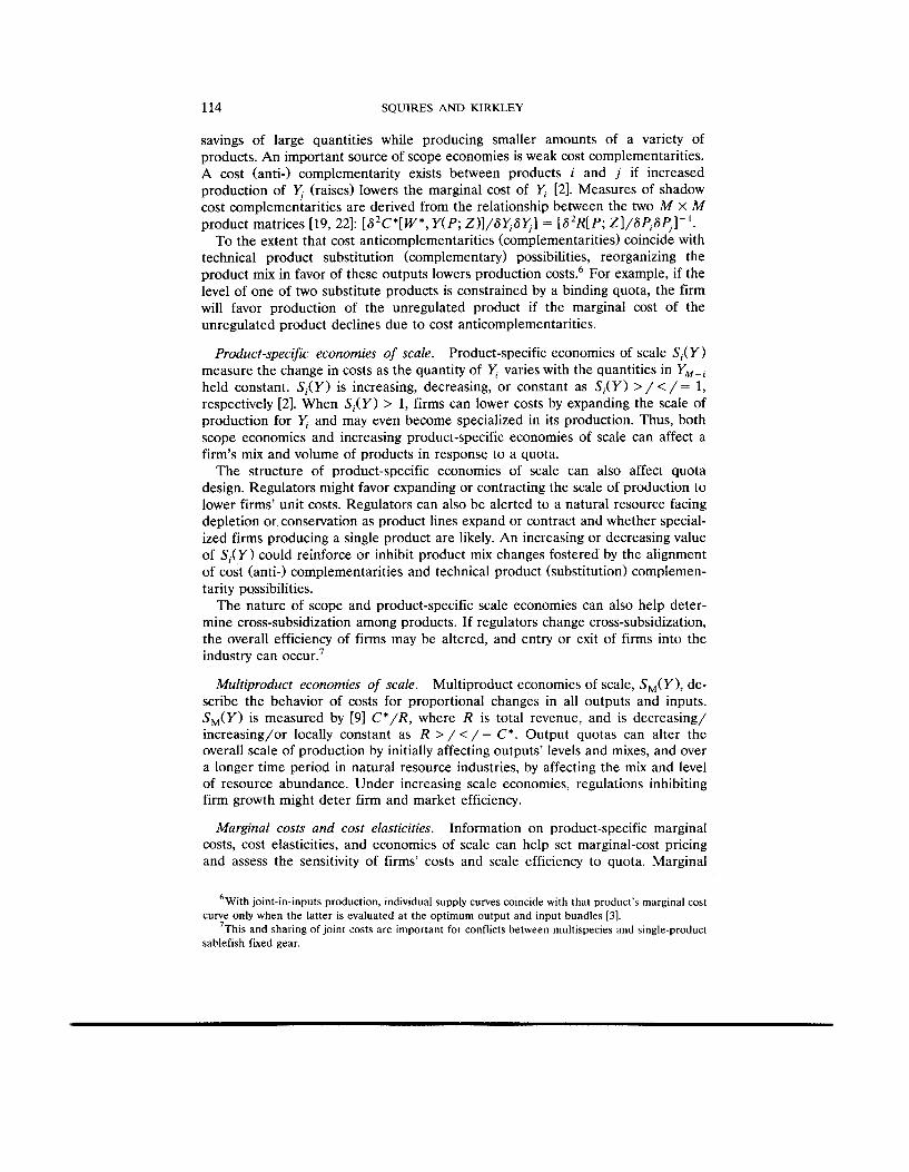
114 SQUIRES AND KIRKLEY
savings of large quantities while producing smaller amounts of a variety of products. An important source of scope economies is weak cost complementarities. A cost (anti-) complementarity exists between products i and j if increased production of 7 (raises) lowers the marginal cost of r, [2]. Measures of shadow cost complementarities are derived from the relationship between the two M X M product matrices [19, 221: [S2C*[W*, Y ( P ; Z>l/SU,SU,l = [6 2R[P; Z]/SP,SP,-’ .
To the extent that cost anticomplementarities (complementarities) coincide with technical product substitution (complementary) possibilities, reorganizing the product mix in favor of these outputs lowers production costs.6 For example, if the level of one of two substitute products is constrained by a binding quota, the firm will favor production of the unregulated product if the marginal cost of the unregulated product declines due to cost anticomplementarities.
Product-specific economies of scale. Product-specific economies of scale S,(Y) measure the change in costs as the quantity of Y, varies with the quantities in YM-, held constant. S , ( Y ) is increasing, decreasing, or constant as S,(Y) > / < / = 1, respectively [2]. When S , ( Y ) > 1, firms can lower costs by expanding the scale of production for Y, and may even become specialized in its production. Thus, both scope economies and increasing product-specific economies of scale can affect a firm’s mix and volume of products in response to a quota.
The structure of product-specific economies of scale can also affect quota design. Regulators might favor expanding or contracting the scale of production to lower firms’ unit costs. Regulators can also be alerted to a natural resource facing depletion or conservation as product lines expand or contract and whether special- ized firms producing a single product are likely. An increasing or decreasing value of S , ( Y ) could reinforce or inhibit product mix changes fostered by the alignment of cost (anti-) complementarities and technical product (substitution) complemen- tarity possibilities.
The nature of scope and product-specific scale economies can also help deter- mine cross-subsidization among products. If regulators change cross-subsidization, the overall efficiency of firms may be altered, and entry or exit of firms into the industry can O C C U ~ . ~
Multiproduct economies of scale. Multiproduct economies of scale, SM( Y ) , de- scribe the behavior of costs for proportional changes in all outputs and inputs. S M ( Y ) is measured by [9] C * / R , where R is total revenue, and is decreasing/ increasing/or locally constant as R > / < / = C * . Output quotas can alter the overall scale of production by initially affecting outputs’ levels and mixes, and over a longer time period in natural resource industries, by affecting the mix and level of resource abundance. Under increasing scale economies, regulations inhibiting firm growth might deter firm and market efficiency.
Marginal costs and cost elasticities. Information on product-specific marginal costs, cost elasticities, and economies of scale can help set marginal-cost pricing and assess the sensitivity of firms’ costs and scale efficiency to quota. Marginal
6With joint-in-inputs production, individual supply curves coincide with that product’s marginal cost
’This and sharing of joint costs are important for conflicts between multispecies and single-product curve only when the latter is evaluated at the optimum output and input bundles [3].
sablefish fiwed gear.
FISHERIES PRODUCTION QUOTA 115
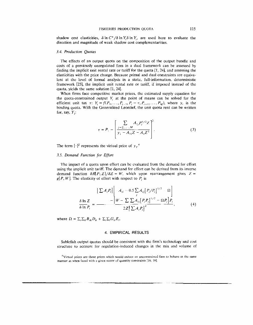
shadow cost elasticities, S In C*/S In YS In k;, are used here to evaluate the direction and magnitude of weak shadow cost complementarities.
3.4. Production Quotas
The effects of an output quota on the composition of the output bundle and costs of a previously unregulated firm in a dual framework can be assessed by finding the implicit unit rental rate or tariff for the quota [l, 241, and assessing the elasticities with the price change. Because primal and dual constraints are equiva- lent at the level of formal analysis in a static, full-information, deterministic framework [23], the implicit unit rental rate or tariff, if imposed instead of the quota, yields the same solution [l, 241.
When firms face competitive market prices, the estimated supply equation for the quota-constrained output at the point of means can be solved for the efficient unit tax T: Y, = f ( P , , . . . , PI- , , PI - T , . . , P M ) , where yI is the binding quota. With the Generalized Leontief, the unit quota rent can be written for, say, Yl :
c
The term [.I2 represents the virtual price of yI.'
3.5. Demand Function for Effort
The impact of a quota upon effort can be evaluated from the demand for effort using the implicit unit tariff. The demand for effort can be derived from its inverse demand function SR[ P ; Z]/SZ = W, which upon rearrangement gives Z =
g[ P, W]. The elasticity of effort with respect to PI is
where R = C I C k B l k D k + C,C,G,,E,.
4. EMPIRICAL RESULTS
Sablefish output quotas should be consistent with the firm's technology and cost structure to account for regulation-induced changes in the mix and volume of
'Virtual prices are those prices which would induce an unconstrained firm to behave in the same manner as when faced with a given vector of quantity constraints [16. 181.
116 SQUIRES AND KIRKLEY
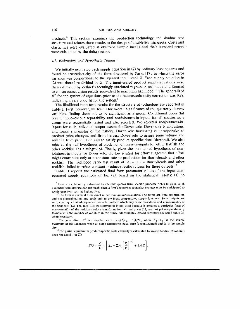
products.' This section examines the production technology and shadow cost structure and relates these results to the design of a sablefish trip quota. Costs and elasticities were evaluated at observed sample means and their standard errors were calculated by the delta method.
4.1. Estimation and Hypothesis Testing
We initially estimated each supply equation in ( 2 ) by ordinary least squares and found heteroscedasticity of the form discussed by Parks [17], in which the error variance was proportional to the squared input level Z. Each supply equation in ( 2 ) was therefore divided by Z. The input-scaled product supply equations were then estimated by Zellner's seemingly unrelated regression technique and iterated to convergence, giving results equivalent to maximum likelihood.'" The generalized R 2 for the system of equations prior to the heteroscedasticity correction was 0.99, indicating a very good fit for the system."
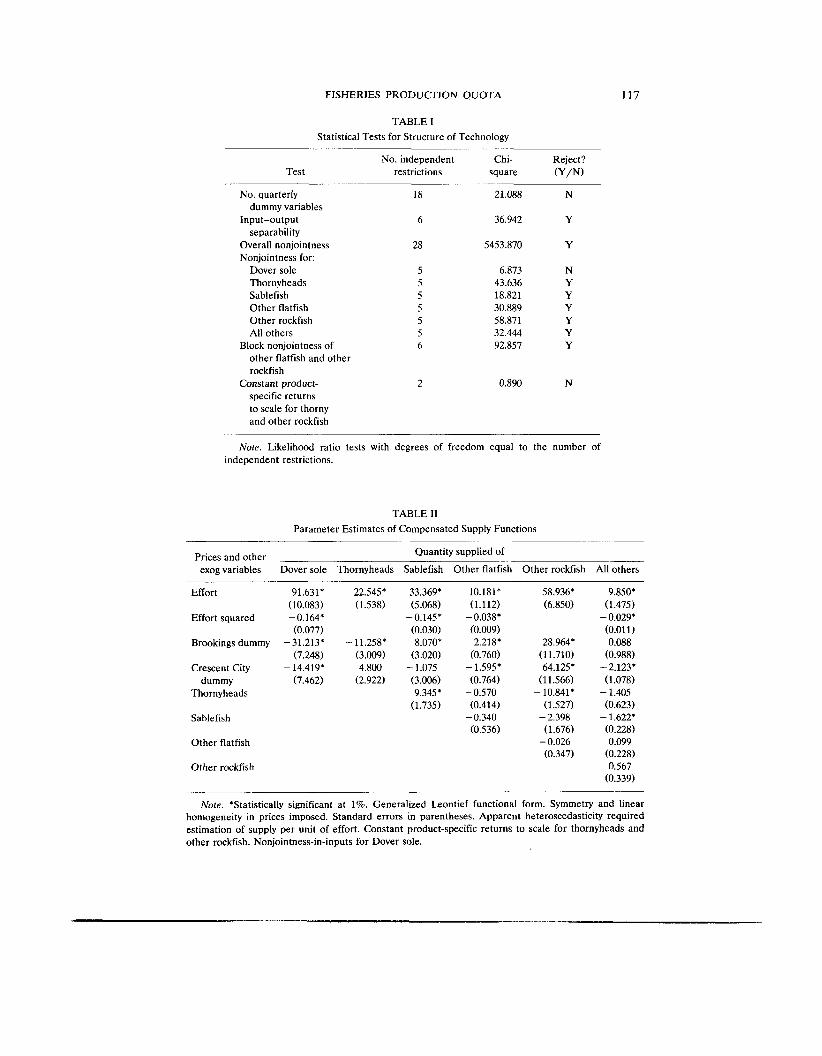
The likelihood ratio tests results for the structure of technology are reported in Table I. First, however, we tested for overall significance of the quarterly dummy variables, finding them not to be significant as a group. Conditional upon this result, input-output separability and nonjointness-in-inputs for all species as a group were sequentially tested and also rejected. We rejected nonjointness-in- inputs for each individual output except for Dover sole. Dover sole is ubiquitous, and forms a mainstay of the fishery. Dover sole harvesting is unresponsive to product price changes, and firms harvest Dover sole to assure some volume and revenue from production and to satisfy product specifications (demand). We also rejected the null hypotheses of block nonjointness-in-inputs for other flatfish and other rockfish (as a subgroup). Finally, given the maintained hypothesis of non- jointness-in-inputs for Dover sole, the low t-ratios for effort suggested that effort might contribute only at a constant rate to production for thornyheads and other rockfish. The likelihood ratio test result of A , = 0, i = thornyheads and other rockfish, failed to reject constant product-specific returns for these outputs."
Table I1 reports the estimated final form parameter values of the input-com- pensated supply equations of Eq. (2), based on the statistical results: (1) no
'Fishery regulation by individual transferable quotas (firm-specific property rights to given catch quantities) can also use our approach, since a firm's responses to market changes must be anticipated to tackle questions such as highgrading.
"The form is assumed to be exact rather than an approximation. The errors are from optimization and not approximation, and apply only to the input-compensated supply functions. Some outputs are zero, creating a limited-dependent variable problem which may cause biasedness and non-normality of the residuals [12]. The Box-Cox transformation is not used because it assumes a particular form of non-normality of the residuals before transformation. Virtual prices [I 1 1 are not yet cornputationally feasible with the number of variables in this study. All estimates instead substitute the small value 0.1 when necessary.
"The generalized R 2 is computed as 1 - exp[2(Lo - L,),"], where Lo ( L , ) is the sample maximum of log-likelihood when all slope coefficients equal zero (unconstrained) and N is the sample size.
The partial equilibrium product-specific scale elasticity is calculated following Kirkley [6 ] (where i does not equal j in E )
12
FISHERIES PRODUCTION QUOTA 117
TABLE I Statistical Tests for Structure of Technology
No. independent Chi- Reject? Test restrictions square (Y/N)
No. quarterly dummy variables
Input-output separability
Overall nonjointness Nonjointness for:
Dover sole Thornyheads Sablefish Other flatfish Other rockfish All others
other flatfish and other rockfish
Constant product- specific returns to scale for thorny and other rockfish
Block nonjointness of
18
6
28
2
21.088
36.942
5453.870
6.873 43.636 18.821 30.889 58.871 32.444 92.857
0.890
N
Y
Y
N
Note. Likelihood ratio tests with degrees of freedom equal to the number of independent restrictions.
TABLE I1 Parameter Estimates of Compensated Supply Functions
Quantity supplied of Prices and other exog variables Dover sole Thornyheads Sablefish Other flatfish Other rockfish All others
Effort
Effort squared
Brookings dummy
Crescent City dummy
Thornyheads
Sablefish
91.631* (10.083)
(0.077)
(7.248)
(7.462)
-0.164*
-31.213* -
- 14.419*
22.545* 33.369* (1.538) (5.068)
- 0.145* (0.030)
(3.009) (3.020) 4.800 -1.075
(2.922) (3.006) 9.345*
(1.735)
- 11.258* 8.070*
10.181* (1.112) - 0.038* (0.009) 2.218*
(0.760) - 1.595* (0.764)
(0.414)
(0.536)
-0.570
- 0.340
Other flatfish
Other rockfish
58.936* (6.850)
28.964* (11.710) 64.125*
(1 1 S66)
(1.527)
(1.676)
(0.347)
- 10.841*
- 2.398
- 0.026
9.850* (1.475) - 0.029' (0.01 1) 0.088
(0.988) -2.123* (1.078)
(0.623)
(0.228) 0.099
(0.228) 0.567
(0.339)
- 1.405
- 1.622:
Note. 'Statistically significant at 1%. Generalized Leontief functional form. Symmetry and linear homogeneity in prices imposed. Standard errors in parentheses. Apparent heteroscedasticity required estimation of supply per unit of effort. Constant product-specific returns to scale for thornyheads and other rockfish. Nonjointness-in-inputs for Dover sole.
118 SQUIRES AND KIRKLEY
quarterly dummy variables; (2) nonjointness-in-inputs for Dover sole (no price terms for it); and (3), constant product-specific returns to scale for thornyheads and other rockfish (no effort squared terms for these outputs).
4.2. Optimal Fishing Effort
The statistical significance of departure of the service ( W ) and shadow ( W * ) prices of Z may be assessed by a t-test. If the null hypothesis of W * = W is not rejected, then shadow costs, C*[W*, Y ( P ; Z ) ] = W * Z , equal full static equilibrium costs, C[W, Y(W, P ) ] = C[W, PI = WZ*(P , W ) , for the profit-maximizing firm. However, the shadow and full static equilibrium multiproduct cost structures (such as scope economies) differ because the long-run expansion effect of Z * ( P , W ) is not incorporated into the shadow cost structure; the Appendix provides further results. The result from this t-test also provides equivalent information on the significance of departures between observed ( Z ) and optimal ( Z * ) levels of the quasi-fixed factor, effort [8].
The t-test of the null hypothesis follows Kulatilaka [81. The shadow price of Z is 6 R [ P ; Z ] / 6 Z = W * , using the observed value of Z and the final form of the technology. The rental price of Z tested against W* is the 1984 capital services price in units of vessel GRT per trip, derived from vessel acquisition prices in confidential financial statements. The estimated t-statistic is 0.06, where the standard error is calculated by the delta method, and indicates that W = W*, Z = Z * ( P , W ) , and C*[W*, Y ( P ; Z ) ] = C[W, Y ( W , P ) ] . Because the paper’s focus is upon the revenue function and input-compensated supply elasticities, the multiproduct shadow cost structure is evaluated. These results also indicate that the firm’s measure of economic capacity utilization equals one, and hence, the firm has no incentives for investment or disinvestment.
4.3. Production Technology
A sablefish quota places the vertical quota supply curve to the left of the unregulated firm’s equilibrium level of sablefish catch, intersecting the catch supply curve at the point corresponding to the quota. The supply curve for the quota is for landings rather than catch; i.e., fish can be discarded at sea.
There are two ways in which sablefish catch can match that of quota (landings): (1) a reallocation of the existing (and constant) level of effort during a trip towards other species, so that the firm moves down the sablefish conditional supply curve from the intersection point of the market equilibrium output price to that of the virtual price (where the quota intersects the catch supply) and along the product transformation surface, changing the product mix; (2) over a longer time period, a reduction of effort (not necessarily to the long-run optimum level) in response to quota, shifting the entire sablefish catch supply curve and lowering the level of all products in a normal technology. We consider each of these in turn.
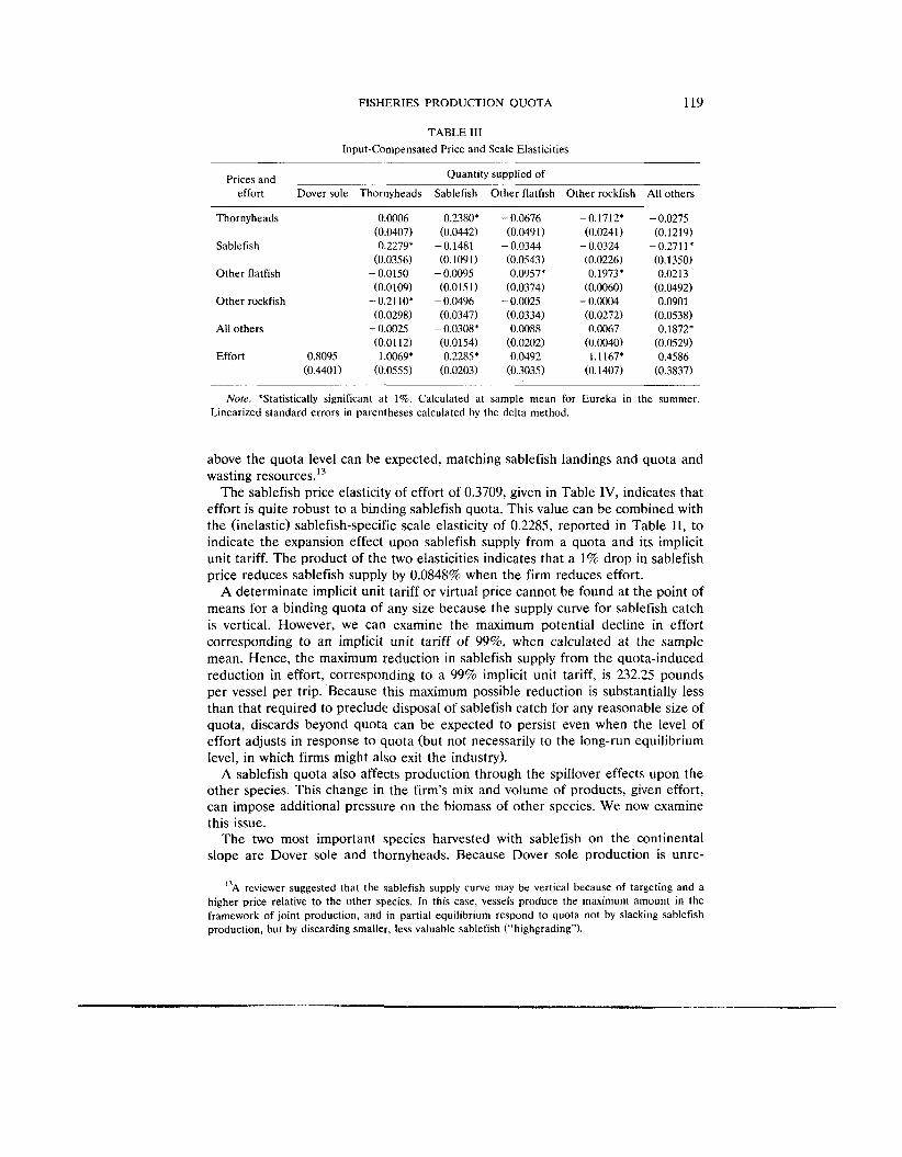
The statistically insignificant own-price sablefish elasticity reported in Table 111 indicates that the conditional sablefish supply curve for catch is vertical. A quota will not directly reduce the quantity supplied of sablefish by movement down the supply curve to the quota quantity during a fishing trip, since there is not an intersection of the two curves. Hence, the firm will not reallocate effort from sablefish production towards other species. At-sea disposal of sablefish catch
FISHERIES PRODUCTION QUOTA 119
TABLE I11 Input-Compensated Price and Scale Elasticities
Quantity supplied of Prices and effort Dover sole Thornyheads Sablefish Other flatfish Other rockfish All others
Thornyheads 0.0006 (0.0407)
Sablefish 0.2279* (0.0356)
Other flatfish - 0.0150 (0.0109)
Other rockfish - 0.21 10* (0.0298)
All others - 0.0025 (0.0112)
Effort 0.8095 1.0069* (0.4401) (0.0555)
0.2380* (0.0442)
(0.1091)
(0.01 5 1)
(0.0347)
(0.0154) 0.2285*
(0.0203)
- 0.1481
- 0.0095
- 0.0496
- 0.0308*
- 0.0676 (0.0491)
(0.0543) 0.0957*
(0.0374) - 0.0025 (0.0334) 0.0088
(0.0202) 0.0492
(0.3035)
- 0.0344
-0.1712* -0.0275 (0.0241) (0.121 9)
(0.0226) (0.1350) 0.1973* 0.0213
(0.0060) (0.0492) - 0.0004 0.0901 (0.0272) (0.0538) 0.0067 0.1872*
(0.0040) (0.0529) 1.1167* 0.4586
(0.1407) (0.3837)
- 0.0324 - 0.2711 *
Note. *Statistically significant at 1%. Calculated at sample mean for Eureka in the summer. Linearized standard errors in parentheses calculated by the delta method.
above the quota level can be expected, matching sablefish landings and quota and wasting resources.13
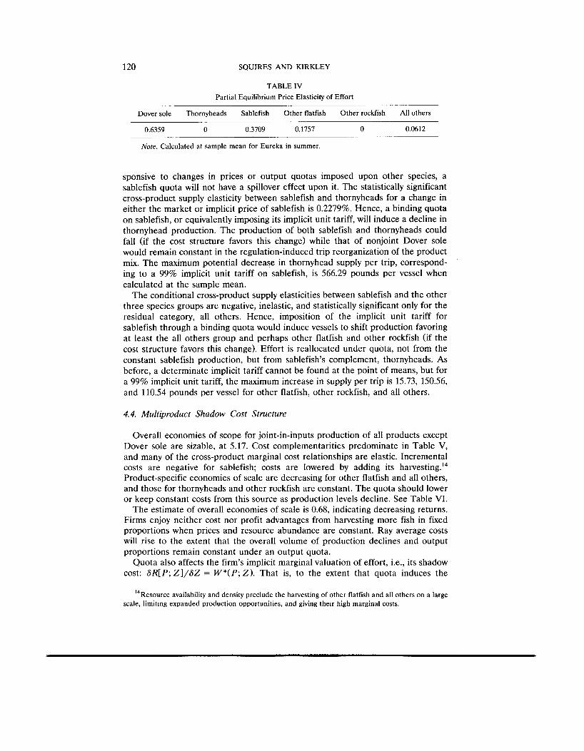
The sablefish price elasticity of effort of 0.3709, given in Table IV, indicates that effort is quite robust to a binding sablefish quota. This value can be combined with the (inelastic) sablefish-specific scale elasticity of 0.2285, reported in Table 11, to indicate the expansion effect upon sablefish supply from a quota and its implicit unit tariff. The product of the two elasticities indicates that a 1% drop in sablefish price reduces sablefish supply by 0.0848% when the firm reduces effort.
A determinate implicit unit tariff or virtual price cannot be found at the point of means for a binding quota of any size because the supply curve for sablefish catch is vertical. However, we can examine the maximum potential decline in effort corresponding to an implicit unit tariff of 99%, when calculated at the sample mean. Hence, the maximum reduction in sablefish supply from the quota-induced reduction in effort, corresponding to a 99% implicit unit tariff, is 232.25 pounds per vessel per trip. Because this maximum possible reduction is substantially less than that required to preclude disposal of sablefish catch for any reasonable size of quota, discards beyond quota can be expected to persist even when the level of effort adjusts in response to quota (but not necessarily to the long-run equilibrium level, in which firms might also exit the industry).
A sablefish quota also affects production through the spillover effects upon the other species. This change in the firm’s mix and volume of products, given effort, can impose additional pressure on the biomass of other species. We now examine this issue.
The two most important species harvested with sablefish on the continental slope are Dover sole and thornyheads. Because Dover sole production is unre-
13 A reviewer suggested that the sablefish supply curve may be vertical because of targeting and a higher price relative to the other species. In this case, vessels produce the maximum amount in the framework of joint production, and in partial equilibrium respond to quota not by slacking sablefish production, but by discarding smaller, less valuable sablefish (“highgrading”).
120 SQUIRES AND KIRKLEY
TABLE IV Partial Equilibrium Price Elasticity of Effort
Dover sole Thornyheads Sablefish Other flatfish Other rockfish All others
0.6359 0 0.3709 0.1757 0 0.0612
Note. Calculated at sample mean for Eureka in summer.
sponsive to changes in prices or output quotas imposed upon other species, a sablefish quota will not have a spillover effect upon it. The statistically significant cross-product supply elasticity between sablefish and thornyheads for a change in either the market or implicit price of sablefish is 0.2279%. Hence, a binding quota on sablefish, or equivalently imposing its implicit unit tariff, will induce a decline in thornyhead production. The production of both sablefish and thornyheads could fall (if the cost structure favors this change) while that of nonjoint Dover sole would remain constant in the regulation-induced trip reorganization of the product mix. The maximum potential decrease in thornyhead supply per trip, correspond- ing to a 99% implicit unit tariff on sablefish, is 566.29 pounds per vessel when calculated at the sample mean.
The conditional cross-product supply elasticities between sablefish and the other three species groups are negative, inelastic, and statistically significant only for the residual category, all others. Hence, imposition of the implicit unit tariff for sablefish through a binding quota would induce vessels to shift production favoring at least the all others group and perhaps other flatfish and other rockfish (if the cost structure favors this change). Effort is reallocated under quota, not from the constant sablefish production, but from sablefish's complement, thornyheads. As before, a determinate implicit tariff cannot be found at the point of means, but for a 99% implicit unit tariff, the maximum increase in supply per trip is 15.73, 150.56, and 110.54 pounds per vessel for other flatfish, other rockfish, and all others.
4.4. Multiproduct Shadow Cost Structure
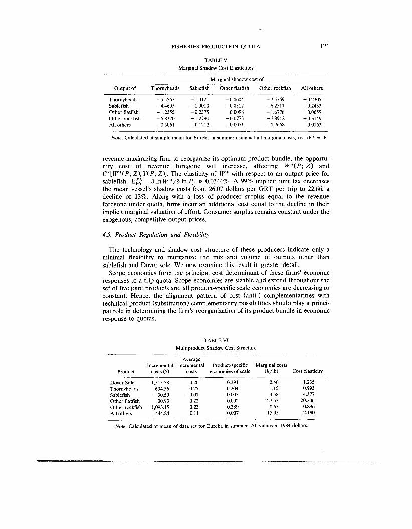
Overall economies of scope for joint-in-inputs production of all products except Dover sole are sizable, at 5.17. Cost complementarities predominate in Table V, and many of the cross-product marginal cost relationships are elastic. Incremental costs are negative for sablefish; costs are lowered by adding its harve~ting.'~ Product-specific economies of scale are decreasing for other flatfish and all others, and those for thornyheads and other rockfish are constant. The quota should lower or keep constant costs from this source as production levels decline. See Table VI.
The estimate of overall economies of scale is 0.68, indicating decreasing returns. Firms enjoy neither cost nor profit advantages from harvesting more fish in fixed proportions when prices and resource abundance are constant. Ray average costs will rise to the extent that the overall volume of production declines and output proportions remain constant under an output quota.
Quota also affects the firm's implicit marginal valuation of effort, i.e., its shadow cost: 6 R [ P ; Z ] / 6 Z = W * ( P ; 2). That is, to the extent that quota induces the
Resource availability and density preclude the harvesting of other flatfish and all others on a large 14
scale, limiting expanded production opportunities, and giving their high marginal costs.
FISHERIES PRODUCTION QUOTA 121
TABLE V Marginal Shadow Cost Elasticities
Marginal shadow cost of
Output of Thornyheads Sablefish Other flatfish Other rockfish All others
Thornyheads - 5.5562 - 1.0121 - 0.0604 - 7.5769 - 0.2305 Sablefish - 4.4605 - 1.0010 -0.0512 -6.2511 - 0.2433 Other flatfish - 1.2355 - 0.2375 0.0098 - 1.6778 - 0.0659 Other rockfish - 6.8320 - 1.2790 - 0.0773 - 7.8912 -0.3149 All others - 0.5061 -0.1212 - 0.0071 - 0.7668 0.0163
Note. Calculated at sample mean for Eureka in summer using actual marginal costs, i.e., W * = W.
revenue-maximizing firm to reorganize its optimum product bundle, the opportu- nity cost of revenue foregone will increase, affecting W * ( P ; Z ) and C * [ W * ( P ; Z ) , Y ( P ; Z ) ] . The elasticity of W * with respect to an output price for sablefish, E;: = 6 In W*/6 In Pi, is 0.0344%. A 99% implicit unit tax decreases the mean vessel’s shadow costs from 26.07 dollars per GRT per trip to 22.66, a decline of 13%. Along with a loss of producer surplus equal to the revenue foregone under quota, firms incur an additional cost equal to the decline in their implicit marginal valuation of effort. Consumer surplus remains constant under the exogenous, competitive output prices,
4.5. Product Regulation and Flexibility
The technology and shadow cost structure of these producers indicate only a minimal flexibility to reorganize the mix and volume of outputs other than sablefish and Dover sole. We now examine this result in greater detail.
Scope economies form the principal cost determinant of these firms’ economic responses to a trip quota. Scope economies are sizable and extend throughout the set of five joint products and all product-specific scale economies are decreasing or constant. Hence, the alignment pattern of cost (anti-) complementarities with technical product (substitution) complementarity possibilities should play a princi- pal role in determining the firm’s reorganization of its product bundle in economic response to quotas.
TABLE VI Multiproduct Shadow Cost Structure
Product Incremental
costs ($1
Average incremental
costs
Dover Sole Thornyheads Sablefish Other flatfish Other rockfish All others
1,515.58 634.56
30.93 1,093.15
444.84
- 30.50
0.20 0.25
- 0.01 0.22 0.23 0.11
Product-specific economies of scale
0.391 0.204
- 0.002 0.002 0.389 0.007
Marginal costs ($/lb) Cost elasticity
0.46 1.235 1.15 0.993 4.58 4.317
127.53 20.306 0.55 0.896
15.35 2.180
Note. Calculated at mean of data set for Eureka in summer. All values in 1984 dollars.
122 SQUIRES AND KIRKLEY
Sablefish’s cost complementarity and substitute supply with all others, other rockfish, and other flatfish suggest that product mix changes favoring these products maximize revenues under quota but also raise marginal trip costs. Sablefish’s complementarity of marginal cost and product supply with thornyheads suggests that the quota-induced reallocation of (constant) effort from thornyheads to the other joint products lowers both revenues from thornyheads and their marginal cost. Costs should increase for other flatfish and all others due to their decreasing product-specific scale economies.
In sum, the most important economic response by firms to a sablefish trip limit, which considers both the technology and shadow costs, will be only a limited change in the product mix toward all others, possibly other rockfish and other flatfish, and away from thornyheads. Both the cost structure and technology limit the reorganizations in the product line due to the very inelastic cross-product conditional supply elasticities and “misalignment” of the cost structure and tech- nology.
In short, when responding to changing market conditions and output quotas, these firms are not likely to make economic choices that extensively reorganize the volume and mix of their product bundle. An ambitious regulatory plan to induce larger changes in the output bundle than permitted by the firm’s inflexible economic capability will leave the industry in its current state of unacceptably high sablefish discards and mortality.
More specifically, a regulatory program consistent with the flexibility of the firm’s product decision might be effective only for quotas of such a large size as to be meaningless. When biomass levels face more serious harvesting pressures, a tighter quota is required. But this is overly restrictive for the firm’s limited product flexibility and capability to reduce effort, and induces at-sea disposal of sablefish production in excess of the quota.
5. CONCLUDING REMARKS
A command-and-control quota on the individual firm’s production of sablefish may be inappropriate. Production has cropped the biomass to a point where increasingly tight production controls are required to keep harvest rates at the requisite level for year-round production under the existing fleet structure. The firm’s flexibility of product decision is tightly constrained by its technology and cost structure. As the resource deteriorates and the trip quota progressively tightens, the firm cannot sufficiently adjust its product bundle to preclude increasingly large sablefish disposal. At some quota level, the larger or more productive firms, for which the quota consistently binds, will eventually disinvest or exit the fishery. A trip quota effectively becomes a backdoor limited entry program for vessels which are not necessarily the more inefficient.
An alternative management strategy to more effectively target industry harvest- ing levels and induce the least efficient firms to exit the industry is required. License limitation, which limits the number of vessels in the fleet, is one possibility, although an effective vessel buy-back program is required to cap production at the appropriate rate when the industry already faces overcapitalization and excessive firm numbers.
FISHERIES PRODUCTION QUOTA 123
A system of individual transferable quotas (ITQs) presents an alternative which is attracting increasing attention among economists. The command-and-control trip quotas examined in this paper would be endowed with property rights to a production flow from the resource stock [20] and be freely transferable between firms. Firms with cost or capacity advantages could purchase quota from other firms. The industry would reorganize by less efficient firms eventually existing the industry, with a lump sum payment, rather than the larger or most productive firms under the current quota system (vessels which may not be less efficient). Given the firm's limited capabilities to alter its product line in response to quota, the major adjustment to quota for some firms-other than disposal-is exit from the sector. But ITQs more efficiently foster this industry restructuring by the more efficient remaining firms compensating the exiting firms.
Yet ITQs in a multispecies fishery can be hampered by the very same inflexible technology limiting the effectiveness of command-and-control quotas. This would defeat the expected benefits of reduced fish mortality and increased technical and arbitrage efficiency. Moreover, because firm exit is a long-run decision, and often involves sunk costs if alternative fisheries or vessel market for exiting vessels are unavailable, the transition period could be longer than e ~ p e c t e d . ' ~
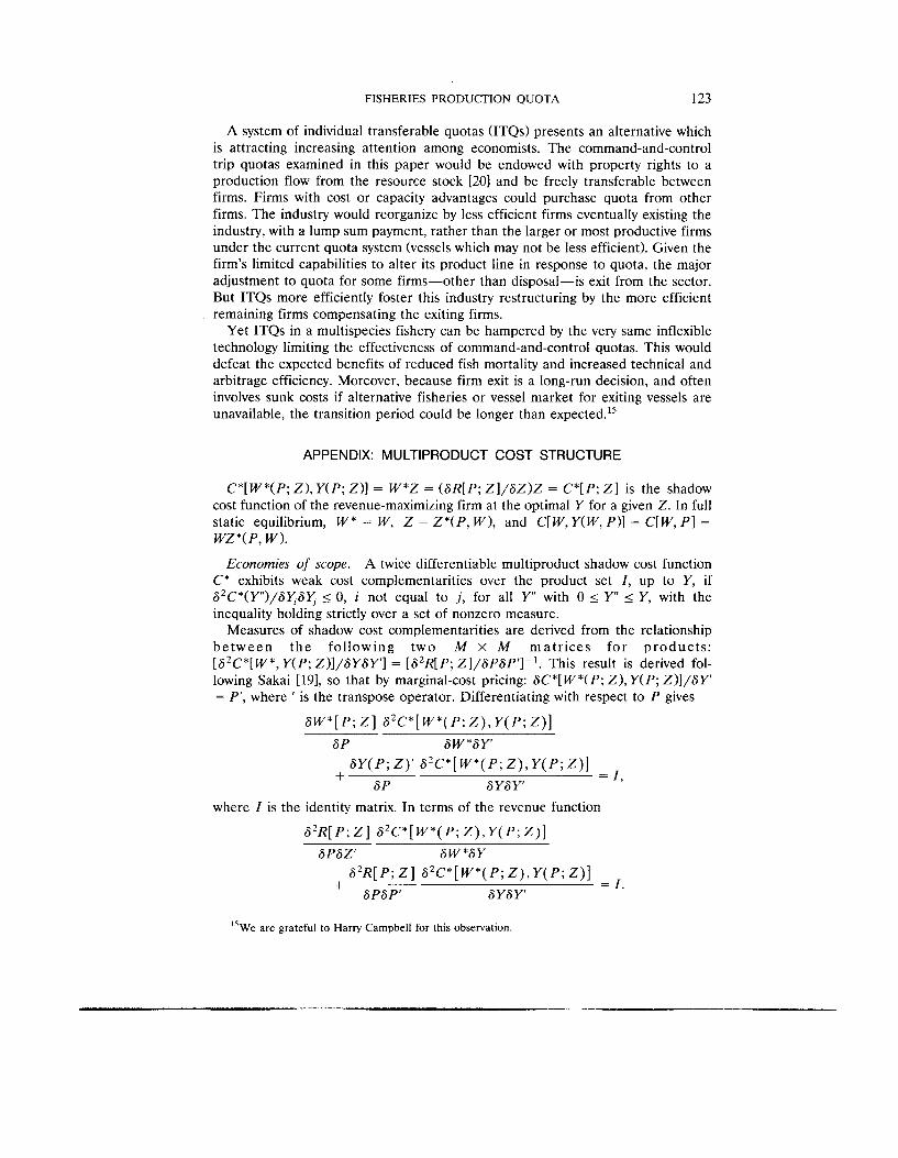
APPENDIX : M U LTI PRODUCT COST STRUCTURE
C*[W*(P; Z ) , Y ( P ; Z ) ] = W*Z = ( 6 R [ P ; Z l /SZ)Z = C*[P; Z l is the shadow cost function of the revenue-maximizing firm at the optimal Y for a given Z. In full static equilibrium, W * = W , Z = Z*(P, W ) , and ClW, Y (W, P)1 = C[W, PI =
A twice differentiable multiproduct shadow cost function C* exhibits weak cost complementarities over the product set I , up to Y , if 62C*(Y) /Sx .6Y, I 0, i not equal to j , for all Y with 0 I Y I Y , with the inequality holding strictly over a set of nonzero measure.
Measures of shadow cost complementarities are derived from the relationship b e t w e e n t h e fo l lowing t w o M X M m a t r i c e s f o r p r o d u c t s : [62C*[W*, Y ( P ; Z)]/6Y6Y'] = [62R[P; Z]/6P6P']- ' . This result is derived fol- lowing Sakai [19], so that by marginal-cost pricing: 6C*[W*(P; Z ) , Y ( P ; Z)] /SY ' = P', where ' is the transpose operator. Differentiating with respect to P gives
WZ*(P, W ) .
Economies of scope.
6W*[ P ; z ] 62C*[ W * ( P ; Z ) , Y ( P ; Z ) ] 6P 6 w *6Y'
+ = I , 6Y( P ; Z ) ' 62C*[ W*( P ; Z ) , Y ( P ; Z ) ]
6P 6Y6Y' where I is the identity matrix. In terms of the revenue function
62R[ P ; Z ] 62C*[ W*( P ; Z ) , Y ( P ; Z ) ] 6P6Z' 6W*6Y
62R[ P ; Z ] 62C*[ W*( P ; Z ) , Y ( P ; Z ) ] = I .
6YSY' +
GPSP'
I5We are grateful to Harry Campbell for this observation.
124 SQUIRES AND KIRKLEY
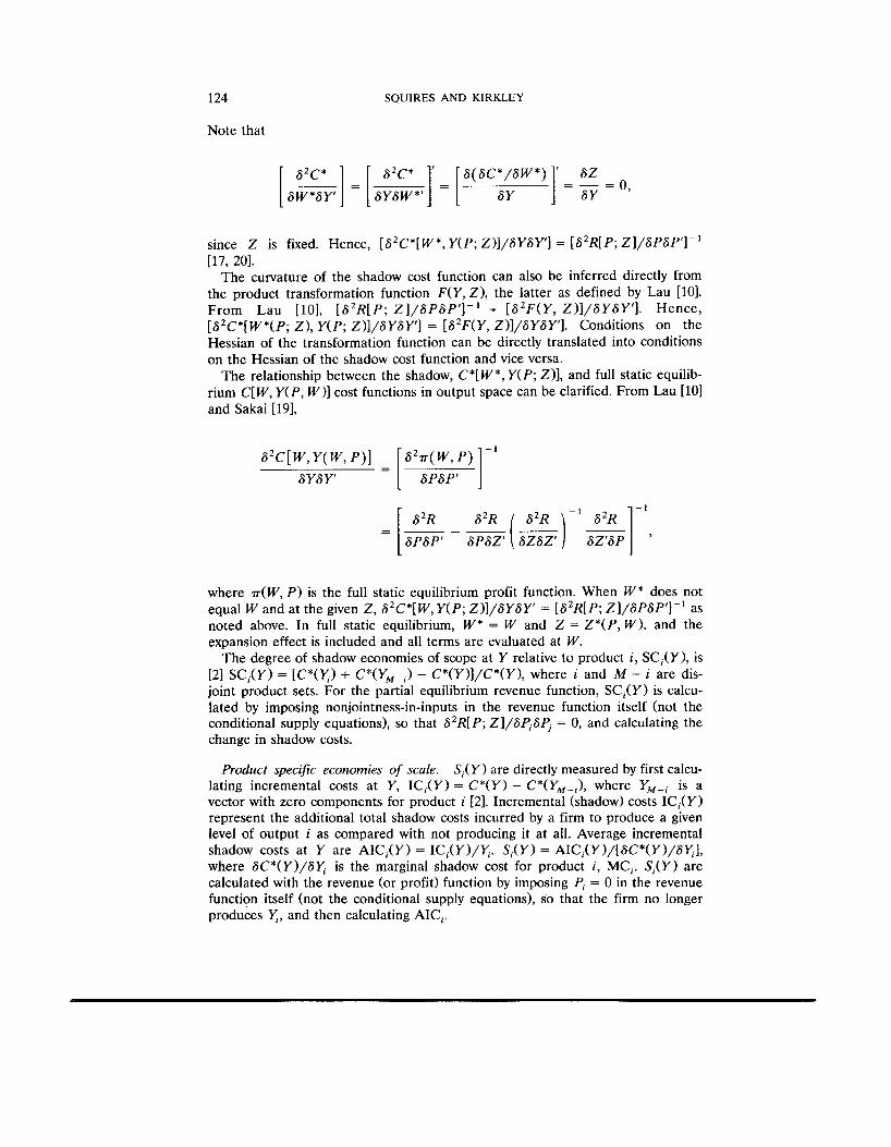
Note that
a2C* 6( SC*/6W*)] ' = _ - 6Z Is"] 6W*6Y' =[-I= 6Y6W*' [ 6Y 6Y - 0,
since 2 is fixed. Hence, [6'C*[W*, Y ( P ; Z)]/6Y6Y'] = [6'R[P; Z]/6p6pf1- ' [17, 201.
The curvature of the shadow cost function can also be inferred directly from the product transformation function F ( Y , Z ) , the latter as defined by Lau [lo]. From Lau [ lo] , [ a 2 R [ P ; Z ] / 6 P 6 P f ] - ' = [6 'F(Y, Z ) ] /6Y6Yf1 . Hence, [6'C*[W*(P; Z ) , Y ( P ; Z)I/SY6Y'] = [6'F(Y, Z)] /6Y6Y'] . Conditions on the Hessian of the transformation function can be directly translated into conditions on the Hessian of the shadow cost function and vice versa.
The relationship between the shadow, C*[W*, Y ( P ; Z ) ] , and full static equilib- rium C[W, Y ( P , W ) ] cost functions in output space can be clarified. From Lau [lo] and Sakai (191,
- 1 6'C[ W , Y( W , P ) ] 62T( W , P )
6YSY = [ GPSP' ] - 1
6'R ( 6*R ) j l 6zp] 6P6P' 6P6Z' 6Z6Z'
- 9
where T(W, P ) is the full static equilibrium profit function. When W * does not equal W and at the given Z , 6'C*[W, Y ( P ; Z)l/6Y6Y' = [ij2R[P; Zl/6P6P']-' as noted above. In full static equilibrium, W * = W and Z = Z*(P, W ) , and the expansion effect is included and all terms are evaluated at W .
The degree of shadow economies of scope at Y relative to product i , SC,(Y), is [2] SC,(Y) = [C*(Y,) + C*(Y,-,) - C*(Y)l /C*(Y) , where i and M - i are dis- joint product sets. For the partial equilibrium revenue function, SC,(Y) is calcu- lated by imposing nonjointness-in-inputs in the revenue function itself (not the conditional supply equations), so that 62R[ P; Z]/6P16P, = 0, and calculating the change in shadow costs.
Product specific economies of scale. S , ( Y ) are directly measured by first calcu- lating incremental costs at Y, IC,(Y) = C * ( Y ) - C*(Y,-,), where Y,-, is a vector with zero components for product i [2]. Incremental (shadow) costs IC,(Y) represent the additional total shadow costs incurred by a firm to produce a given level of output i as compared with not producing it at all. Average incremental shadow costs at Y are AIC,(Y) = IC,(Y)/Y,. S , (Y) = AICl(Y)/[6C*(Y>/6Y,1, where 6 C * ( Y ) / 6 x is the marginal shadow cost for product i , MC,. S , ( Y ) are calculated with the revenue (or profit) function by imposing P, = 0 in the revenue function itself (not the conditional supply equations), so that the firm no longer produces x, and then calculating AIC,.
FISHERIES PRODUCTION QUOTA 125
Multiproduct economies of scale. S,(Y) is measured by C*/R, where C* = W*Z in partial equilibrium [9], where R is total revenue. As R > / < / = total shadow costs, S,(Y) is decreasing/increasing/or locally constant [2].
Marginal shadow costs and shadow cost elasticities. MC, at Y(P; Z ) with the partial equilibrium revenue function is calculated from the shadow cost equation C* = W*Z, i.e., MC, = 6C*(Y)/6k;. The shadow cost elasticity, which indicates the change in total shadow costs for a change in product i , is 6 In C * / 6 In k; =
( Y ; MC,)/C* = [k;S(W*Z)/Sk;]/[ZW*]. Partial equilibrium marginal shadow cost elasticities are calculated using the
M x M matrix [6*R(P; Z]/6P16P,]-’, so that the marginal shadow cost elasticity for product i becomes [6‘R[P; Z]/6P,6P,]-’ (Y/MC,), i , j E M . Own marginal shadow cost elasticities indicate the slopes of marginal shadow cost curves.
REFERENCES
1. J. E. Anderson, The relative efficiency of quotas: The cheese case, Amer. Econom. Reu. 75,
2. W. Baumol, J. Panzar, and R. Willig, “Contestable Markets and the Theory of Industry Structure,”
3. B. Beattie and C. Taylor, “The Economics of Production”, Wiley, New York (1985). 4. W. E. Diewert, Functional forms for revenue and factor requirements functions, Internat. Econom.
5. R. Hall, The specification of technology with several kinds of output, J . Polit. Economy 81,
6. J. Kirkley, “The Relationship between Management and the Technology in a Multi-species Fishery: The New England, Georges Bank, Multi-species Fishery”, Ph.D. dissertation, University of Maryland (1986).
7. J. Kirkley and I. Strand, Jr., The technology and management of multispecies fisheries, Appl. Econom. 20, 1279-1302 (1988).
8. N. Kulatilka, Are observed technologies at long-run equilibrium? J . Econometrics 25, 253-268 (1985).
9. K. Laitinen, “A Theory of the Multiproduct Firm,” North-Holland, Amsterdam (1980).
178-190 (1985).
Harcourt Brace Jovanovich, San Diego (1982).
Reu. 15, 119-130 (1974).
878-892 (1973).
10. L. Lau, A characterization of the normalized restricted profit function, J . Econom. Theory 12, 131-163 (1976).
11. L. Lee and M. Pitt, Microeconometric demand systems with binding nonnegativity constraints: The dual approach, Econometrica 54, 1237-1242 (1986).
12. G . S. Maddala, “Limited Dependent and Qualitative Variables in Econometrics,” Cambridge Univ. Press, Cambridge, U.K. (1984).
13. L. Mahe and H. Guyomard, Supply behavior with production quota and quasi-fixed factors, memo, Institut National de la Recherche Agronomique, Station d’Economie Rurale, France (1989).
14. D. McFadden, Cost, revenue, and profit functions, in “Production Economics: A Dual Approach to Theory and Applications” (M. Fuss and D. McFadden, Eds.), Vol. I, North-Holland, Amster- dam (1978).
15. G. Moshini, A model of production with supply management for the Canadian agricultural sector, Amer. J . Agr. Econom. 70, 318-329 (1988).
16. J. Neary and K. Roberts, The theory of household behavior under rationing, European Econom. Reu. 13, 24-42 (1980).
17. R. Parks, Price responsiveness of factor utilization in Swedish manufacturing, Reu. Econom. Statist. 53, 129-139 (1970).
18. E. Rothbarth, The measurement of changes in real income under conditions of rationing, Reu. Econom. Stud. 8, 100-107 (1941).
19. Y. Sakai, Substitution and expansion effects in production theory: The case of joint production, J . Econom. Theory 9, 225-274 (1974).

126 SQUIRES AND KIRKLEY
20. A. Scott, Catch quotas and shares in the fishstock as property rights, in “Natural Resource Economics and Policy Applications” (E. Miles et al., Eds.), U. of Washington Press, Seattle (1986).
21. D. Squires, Public regulation and the structure of production in multiproduct industries, Rand J . Econom. 18, 232-247 (1987).
22. D. Squires, Production technology, costs, and multiproduct industry structure, Canad. J . Econom.
23. M. Weitzman, Prices vs. quantities, Rec. Econoni. Stud. 41, 50-65 (1974). 24. A. D. Woodland, “International Trade and K-source Allocation,” North-Holland, Amsterdam
21, 359-378 (1988).
(1982).