productive cities: sorting, selection and agglomeration

Productive cities: Sorting, selection andagglomeration

Kristian Behrens, Gilles Duranton and Frederic Robert-NicoudUQAM, U. of Toronto and U. of Geneva

June 19, 2012

Big cities viewed from space

5

Core-Periphery patterns

Motivation I: Spatial inequalities are ubiquitous

Human settlements and production are spatially concentrated

I Cities are the center of economic activityI e.g. Japan’s 3 core metropolitan areas (NOT)

I cover 5.2% of Japan’s land massI host 33% of its population, 31% of its manuf. employmentI create 40% of its GDPI cover .18% of East Asia’s area but generate 29% of its GDP!

I Likewise, US’s most active countiesI cover 1.5% of US’s land massI represent 41.2% of its manufacturing employment

I Paris metropolitan area (Ile-de-France)I Only 12% of available land is used for housing, plants and

transportation infrastructureI Covers 2.2% of France’s area, 19% of its pop., 30% of its GDPI Ministere de l’egalite des territoires notwithstanding...

Motivation II: Big cities pay big wages

Urban premium

I Wages and productivity are increasing in city size

I Cities attract the most talented people

Earnings inequalities across cities

conditional on ability

99.

29.

49.

69.

810

10.2

log(

mea

n ea

rnin

gs)

10.5 11.5 12.5 13.5 14.5 15.5 16.5log(population)

Figure 1. Size–productivity–ability

5

First aim of our paper (qualitative)

I Provide three possible explanations for urban premium in aunified setting

I AgglomerationI SortingI SelectionI (We omit natural advantage)

Second aim of our paper (quantitative)

I Provide structural interpretation to these slopes (elasticities)

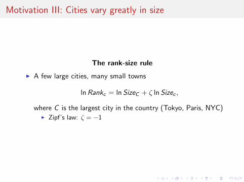
Motivation III: Cities vary greatly in size

The rank-size rule

I A few large cities, many small towns

ln Rankc = ln SizeC + ζ ln Sizec ,

where C is the largest city in the country (Tokyo, Paris, NYC)I Zipf’s law: ζ = −1

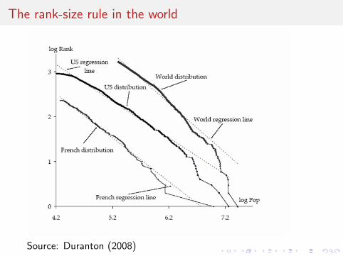
The rank-size rule in the world

Source: Duranton (2008)

Third aim of our paper

I Provide an original explanation for Zipf’s law

Plan

I Balancing agglomeration economies and congestion: TheHenderson model

I Adding selection and ability sorting across cities: our model

I Equilibrium with talent-homogenous cities

I Zipf’s law

I Quantitative implications

The Henderson model of cities (American Ec. Rev. 1974)

I Agglomeration economies at the local/urban levelI Many explanations are plausible, many economic mechanisms

have been proposed in the literature (Duranton and Puga2004)

I E.g. input sharing as in Ethier’s (1982) version of Dixit andStiglitz (1977)

I Per-capita output in city c

Yc

Lc= AcLεc ,

where Lc denotes city population and Ac is local TFPI ε captures agglomeration economies and is related to the

mechanism generating local increasing returnsI e.g. ε = 1/(σ − 1) in the Ethier-Dixit-Stiglitz model

Agglomeration economies in the empirical literature

I Positive association between city size and various measures ofproductivity (Recall Figure 1 above for the US)

I Empirically, ε ∈ (0, 0.1)

I This association is causalI IV evidence: Ciccone and Hall (1996), Combes, Duranton,

Gobillon and Roux (2010)I Quasi-experimental evidence: Greenstone, Hornbeck and

Moretti (2010)I Input-output linkages as a key channel (Holmes 1999; Amiti

and Cameron 2007; Ellison, Glaeser and Kerr 2010)

Urban congestion and spatial equilibrium

I Local/urban congestion diseconomiesI CommutingI Competition for the ultimate scarce factor: landI Competition for purely local amenities, goods and servicesI Per capita urban costs are proportional to Lγ

c , where γ is theelasticity of the cost of living with respect to city size

I Spatial equilibrium balances the twoI High wages compensate workers for high urban cost of livingI High worker productivity compensates firms for high wages

I Spatial equilibrium with homogeneous agents

ωc = ω,

for all cities with Lc > 0 (ωc < ω otherwise), some ω > 0

Spatial equilibrium in Henderson’s model

N

Net Wage Curve

N

( )NH

( )Nw

Wage Curve

Cost of Living Curve

( ) ( )NHNw −

Labour Supply Curve

)(a

)(b

)(c

Plan




I Zipf’s law


Productive cities: Sorting, selection and agglomeration

Objectives

I Build a model of a self-organized urban system withI agglomeration economiesI sorting along abilityI selection along productivity

I ExplainI urban premiumI composition and size distribution of cities

I Model consistent with several stylized factsI Provides a static explanation for Zipf’s lawI Allows us to reinterpret extant empirical evidenceI Little sorting but it matters greatly [a puzzle]

I Central message: (γ − ε) is tiny!

Sorting

I Urban premium increasing with skills (Wheeler, 2001; Glaeserand Mare, 2001)

I Sorting matters (Combes, Duranton, Gobillon, 2008)

Agglomeration

I Size-productivity relationship robust to sorting (CDG, 2008)

I Causal impact of city size on productivity

I IO-linkages are an important source (Holmes, 1999; Ellison,Glaeser, Kerr, 2010)

Selection

I Higher survival productivity cutoff in larger markets (Syverson,2004)

I But no selection after controlling for agglomeration andsorting (Combes, Duranton, Gobillon, Puga, Roux, 2012)

Model: Timing

1. Talent t of each agent is revealed (c.d.f. Gt)

2. Agents choose a city

3. Luck s of each agent is revealed (c.d.f. Gs)→ Entrepreneurial productivity is ϕ ≡ t × s (c.d.f. F )

Worker productivity is ϕa

4. Occupational selection (workers vs entrepreneurs)

5. Market clearing, production, consumption

Model: Preferences and technology

Preferences

I Risk-neutral individuals consume one unit of land and a finalconsumption good

Technology

I Two-step production process

I Homogenous aggregate output (freely tradable numeraire) incity c

Yc =

[∫Ω

xc(i)1

1+εdi

]1+ε

produced using local intermediates provided by entrepreneurs

xc(i) = ϕ(i)lc(i), with ϕ(i) = t(i)× s(i)

Market outcome

Solving the model backward

I Solve first for prices, quantities and occupations in each city cI At this stage, individuals take as given:

I location and own productivityI cumulative productivity distribution Fc(·)I city size Lc

I Individuals self-select into either workers or entrepreneursI We impose aε < 1I i.e. productive agents have a comparative advantage in

entrepreneurship

Occupational selection

I Profit maximization yields

π(ϕ) =ε

1 + εY[ϕ

Φ

] 1ε

where Φ ≡[∫

Ωϕ(j)

1εdj

]εI Complementarity between Y and ϕI Offsetting market crowding or toughness via Φ (aggregate city

productivity)

I Agent with productivity ϕ becomes entrepreneur iff

π(ϕ) > wϕa

I yields productivity cutoff for selection into entrepreneurship

ϕ ≡[

Φ

(1 + ε

ε

w

Y

)ε] 11−a ε

City equilibrium

Proposition 1 (existence and selection). Given population, L,and its productivity distribution, F (·), the equilibrium in a cityexists and is unique.

Proposition 2 (agglomeration). Given F (·), larger cities havehigher aggregate productivity, per-capita income, and wages thansmaller cities. Productivity cutoff for selection does not depend oncity size.

Per-capita city income is

Y

L=

(∫ +∞

ϕϕ

1εdF (ϕ)

)ε(∫ ϕ

0ϕadF (ϕ)

)Lε ,

Urban costs

I Standard monocentric city structure

I Commuting costs t(x) ∝ xγ , where γ > ε

I Per-capita urban costs are given by θLγ

Returns to talent are increasing in city size

I Expected utility for individual with talent t

EV (t) =

∫ +∞

0maxw × (ts)a, π(ts)dGs(s)− θLγ

= w ta

[∫ ϕ/t

0sadGs(s) +

(t

ϕ

) 1ε−a∫ +∞

ϕ/ts

1εdGs(s)

]− θLγ

Proposition 3 (complementarity between talent and citypopulation). Conditional of F (·), more talented individualsbenefit disproportionately from being located in larger cities:

∂2EV (t)

∂t∂L

∣∣∣F (.)≥ 0

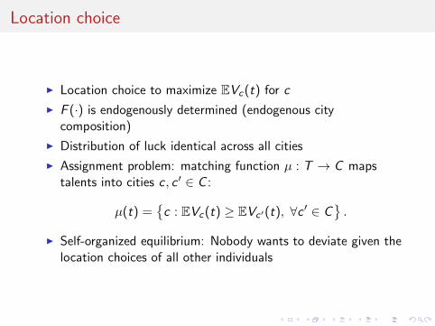
Location choice

I Location choice to maximize EVc(t) for c

I F (·) is endogenously determined (endogenous citycomposition)

I Distribution of luck identical across all cities

I Assignment problem: matching function µ : T → C mapstalents into cities c , c ′ ∈ C :

µ(t) =

c : EVc(t) ≥ EVc ′(t), ∀c ′ ∈ C.

I Self-organized equilibrium: Nobody wants to deviate given thelocation choices of all other individuals

Plan




I Zipf’s law


Talent homogenous cities equilibrium

I Symmetric equilibrium unstable if sufficient heterogeneity intalent

I Consider equilibrium with only one type of talent tc per city(but non-degenerate productivity distribution)

I The productivity cutoff is proportional to talent : ϕc

= S × tcfor some S and all c (easy to show formally)

I i.e. sorting induces selectionI Conditional on sorting, no differences in selection (CDGPR,

2010)

I Assignment problem is tricky since EVc(t) not generallysupermodular in t and L

I At equilibrium, cities can neither be too small (agglomeration)nor too large (congestion)

I Existence of an equilibrium relationship between talent(productivity) and size

6

-

EVc0 (t0)

EVc1 (t1)

EVc1 (t0)

L∗c (tc)

t

L

0

-

?x

x

xEVc2 (t2)

t1t0

L0

L1

Talent homogeneous equilibrium

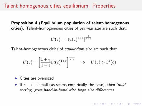
Talent homogenous cities equilibrium: Properties

Proposition 4 (Equilibrium population of talent-homogenouscities). Talent-homogeneous cities of optimal size are such that:

Lo(c) =[ξt(c)1+a

] 1γ−ε

Talent-homogeneous cities of equilibrium size are such that

L∗(c) =

[1 + γ

1 + εξt(c)1+a

] 1γ−ε

⇒ L∗(c) > Lo(c)

I Cities are oversized

I If γ − ε is small (as seems empirically the case), then ‘mildsorting’ goes hand-in-hand with large size differences

Plan




I Zipf’s law


Talent homogenous cities equilibrium: Zipf’s law

Proposition 5 (Number and size distribution of cities). Theequilibrium ‘number’ of cities is proportional to population size Λand too small relative to the social optimum. The size distributionof talent-homogenous cities converges to Zipf’s law regardless ofthe distribution of talent t as η ≡ (γ − ε)/(1 + a)→ 0.

Plan




I Zipf’s law


Quantitative applications and quantitative implications

We use the model to provide structural interpretation of extantregressions and conduct welfare analysis

Estimating γ and ε

I γ is the regression coefficient of ln wc = αI + γ ln Lc + εIcI ε is the regression coefficient of ln wc = αII + ε ln Lc + tc + εIIcI Using US data we find γ = .082 and ε = .051

I Remarkably, γ is also the regression coefficient ofln tc = αIII + γ ln Lc + εIIIc

I For this regression we find γ = .068

Cities are naturally oversized

I by a huge factor (close to Euler’s e)

I but welfare cost of oversize is negligible

I Why? Because γ, ε and (γ − ε) are tiny.

Revisiting the findings of Gennaioli, La Porta, Lopez-de-Silanes,and Shleifer (2012)

I Macro data: 1499 regions of 105 countries

I Regressing output per capita yc on region size and stuff

ln(yc) = ε ln Lc + f (Gt,c(·),Gs(·))

≈ 0.068 log Lc + 0.257 Educc + controlsc + υc

Revisiting the findings of Gennaioli et al. (cont.)

I Extend our model for limited span-of-control (Lucas 1978)

I Micro data: 6314 firms in 76 regions of 20 countries

I Regressing firm revenue Zi on education

ln Zi = 0.126 log Lc(i) + 0.073 Educc(i) + 0.860 Ni + 0.017 EducWi

+0.026EducEi + controlsc(i) + υi

I This implies extremely high returns to education forentrepreneurs in the framework of Gennaioli et al. (26%)

Our interpretation:

I Self-selection of the most talented into entrepreneurship:coefficient on EducE

i is biased upwards

I Self-selection of the least talented into workers: coefficient onEducW

i is biased downwards

A novel interpretation of the finding of Davis and Ortalo-Magne(2011)

I Housing expenditure shares may be constant withoutimposing Cobb-Douglas preferences

Summary

I Agglomeration, selection and sorting interact to explainthe urban premium, the composition, and the size distributionof cities

I Model captures key stylised facts, useful for reinterpretingempirical evidence in a unified framework

I Provides a static explanation for Zipf’s law in Henderson-likemodel

I Provides an explanation for the sorting puzzle

productive cities: sorting, selection and agglomeration

Documents