Productivity and Growth of Japanese Prefectures

Prepared for the 3rd World KLEMS Conference, Tokyo, May 19-20, 2014.

Joji Tokui (Shinshu University and RIETI)Kyoji Fukao (Hitotsubashi University and RIETI)

　　　 Tsutomu Miyagawa (Gakushuin University and RIETI) Kazuyasu Kawasaki (Toyo University)

Tatsuji Makino (Hitotsubashi University)

This presentation is based on our two papers.Joji Tokui, Tatsuji Makino, Kyoji Fukao, Tsutomu Miyagawa, Nobuyuki Arai, Sonoe Arai, Tomohiko Inui, Kazuyasu Kawasaki, Naomi Kodama and Naohiro Noguchi (2013), “Compilation of the Regional-Level Japan Industrial Productivity Database (R-JIP) and Analysis of Productivity Differences across Prefectures,” The Economic Review, Vol. 64 No. 3, pp.218-239 (in Japanese).Kazuyasu Kawasaki, Tsutomu Miyagawa and Joji Tokui (2014), “Reallocation of Production Factors in the Regional Economies in Japan: Towards an Application to the Great East-Japan Earthquake.”

Contents

1. Construction of Regional-Level Japan Industrial Productivity (R-JIP) Database

2. The change in prefectural productivity differences and its causes (1970-2008)

3. Factor reallocation and its efficiency among prefectures and industries

１． Construction of Regional-Level Japan Industrial Productivity (R-JIP) Database

Main Features of R-JIP Database• 47 prefectures in Japan• 23 industries (13 manufacturing + 10 non-

manufacturing)• 1970-2008 (annual data)• Value added, capital input, labor input• Input data are constructed taking quality into account. (1) time-series quality change for both capital and labor (2) cross-sectional quality difference for labor

5

Relationship between R-JIP and JIP

• The control totals of regional-level value added, capital, and labor are 2011 JIP data.• The value added deflator for each industry calculated from the 2011

JIP data is used. • The investment deflator and capital depreciation rate for each

industry calculated from the 2011 JIP data is used.• The capital cost and capital quality for each industry calculated from

the 2011 JIP data are used.• In contrast, we calculate regional-specific working hours, labor costs,

and labor quality for each industry.6

The R-JIP Database is available on RIETI’s website (in Japanese only at the moment)

7

http://www.rieti.go.jp/jp/database/R-JIP2012/

index.html

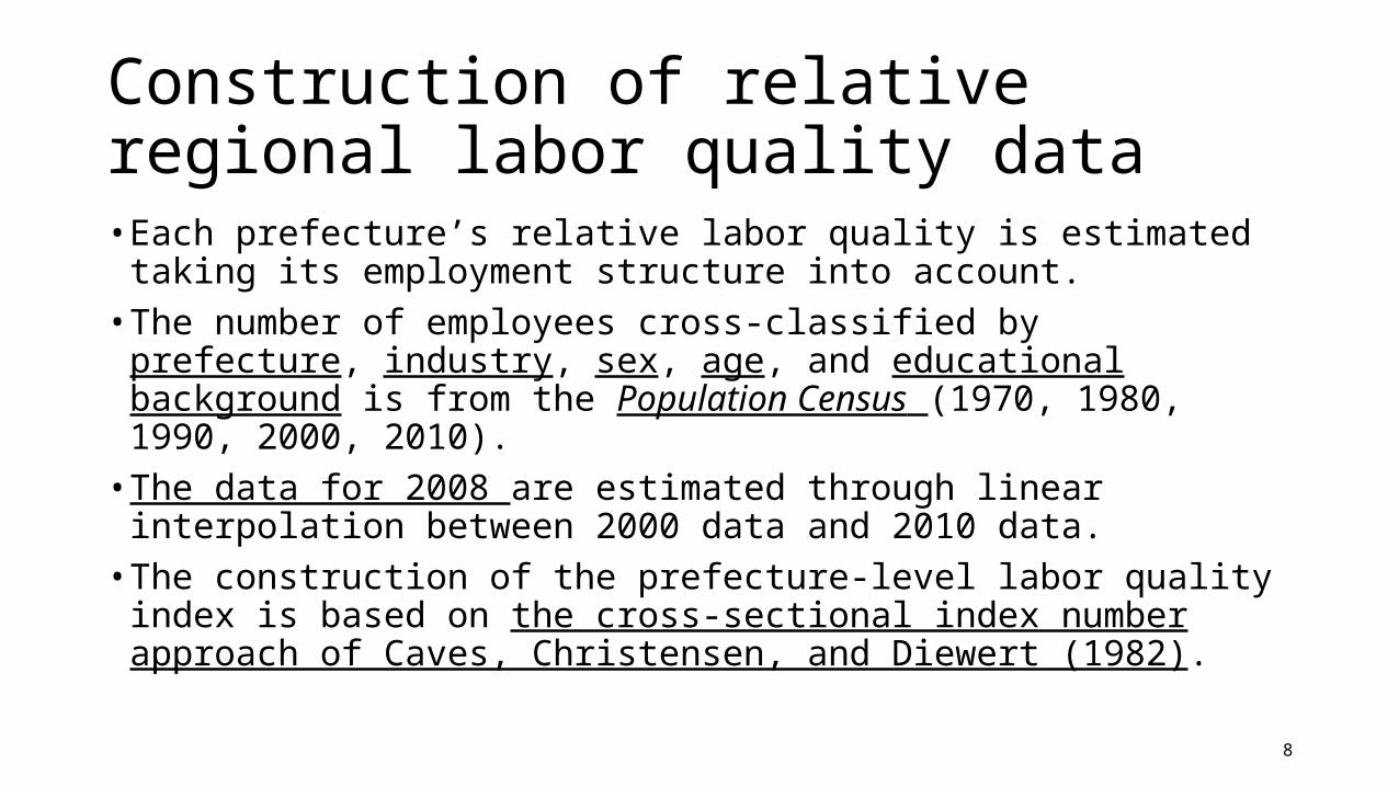
Construction of relative regional labor quality data• Each prefecture’s relative labor quality is estimated taking its

employment structure into account.• The number of employees cross-classified by prefecture, industry, sex,

age, and educational background is from the Population Census (1970, 1980, 1990, 2000, 2010).• The data for 2008 are estimated through linear interpolation between

2000 data and 2010 data.• The construction of the prefecture-level labor quality index is based

on the cross-sectional index number approach of Caves, Christensen, and Diewert (1982).

8

The difference in labor quality across prefectures in 1970 (Tokyo=1)

0.600

0.650

0.700

0.750

0.800

0.850

0.900

0.950

1.000

Toky

oKa

naga

wa

Osa

kaH

yogo

Kyot

oH

irosh

ima

Fuku

oka

Aich

iYa

mag

uchi

Saita

ma

Shiz

uoka

Chib

aW

akay

ama

Oka

yam

aTo

yam

aKa

gaw

aN

ara

Nag

asak

iN

agan

oM

ieEh

ime

Gum

ma

Hok

kaid

oIs

hika

wa

Fuku

iTo

chig

iYa

man

ashi

Gifu

Miy

agi

Shig

aO

itaTo

ttor

iIb

arak

iTo

kush

ima

Saga

Niig

ata

Fuku

shim

aYa

mag

ata

Kum

amot

oSh

iman

eKo

chi

Miy

azak

iAk

itaIw

ate

Kago

shim

aAo

mor

iO

kina

wa

9

The difference in labor quality across prefectures in 2008 (Tokyo=1)

0.600

0.650

0.700

0.750

0.800

0.850

0.900

0.950

1.000

Toky

oKa

naga

wa

Aich

iH

irosh

ima

Osa

kaN

ara

Hyo

goKy

oto

Shig

aTo

yam

aSh

izuo

kaYa

man

ashi

Mie

Yam

aguc

hiKa

gaw

aSa

itam

aO

kaya

ma

Fuku

oka

Gum

ma

Ishi

kaw

aTo

kush

ima

Toch

igi

Fuku

iCh

iba

Ehim

eIb

arak

iG

ifuN

agan

oM

iyag

iO

itaTo

ttor

iW

akay

ama

Shim

ane

Fuku

shim

aSa

gaKu

mam

oto

Yam

agat

aN

iigat

aN

agas

aki

Koch

iH

okka

ido

Akita

Iwat

eM

iyaz

aki

Kago

shim

aO

kina

wa

Aom

ori

10

• Differences in regional labor quality have shrunk in the 40 years since 1970.• But they still remain. Labor quality in the prefecture with the highest

level is 1.3 times that of that with the lowest level.

2. The change in prefectural productivity differences and its causes (1970-2008)

• Some people are commuting across prefectural borders. In that case, the prefecture where they inhabit and where they work are different.• Since in our database value added data are compiled in the prefecture

where production is taken place and labor input data are compiled in the prefecture where they work, we focus on labor productivity instead of the per capita income of each prefecture.

We decompose prefectural labor productivity into three factors: prefectural TFP differences, the capital-labor ratio, and labor quality.

Decomposition of factors underlying regional differences in labor productivity

14

L

i

LirL

iLir

i

Vi

Vir

i

ir

i

irKi

Kir

i

Vi

Vir

iir

Vi

Vir

i i

irVi

Vir

r

Q

QSSSS

H

H

Z

ZSSSS

RTFPSS

H

HSS

V

V

log2

1

2

1

log- log2

1

2

1

2

1

log2

1log

23

1

23

1

23

1

23

1

: Labor Productivity

: TFP Difference

: Capital-Labor Ratio

: Labor Quality

Decomposition of differences in regional labor productivity in 1970 (in logarithm)

15

-0.3

-0.2

-0.1

0.0

0.1

0.2

0.3

0.4

0.5

Kana

gaw

aTo

kyo

Osa

kaM

ieCh

iba

Shig

aYa

mag

uchi

Hyo

goW

akay

ama

Nar

aAi

chi

Oka

yam

aSh

izuo

kaH

irosh

ima

Kyot

oTo

chig

iTo

yam

aSa

itam

aIb

arak

iG

ifuIs

hika

wa

Ehim

eFu

kuok

aG

umm

aO

itaKa

gaw

aN

agan

oAk

itaH

okka

ido

Niig

ata

Toku

shim

aM

iyag

iFu

kui

Saga

Fuku

shim

aTo

ttor

iIw

ate

Aom

ori

Yam

agat

aYa

man

ashi

Miy

azak

iKo

chi

Kum

amot

oN

agas

aki

Kago

shim

aSh

iman

eO

kina

wa

TFP Difference

Capital-Labor Ratio

Labor Quality

Labor Productivity

Decomposition of differences in regional labor productivity in 2008 (in logarithm)

16

-0.3

-0.2

-0.1

0.0

0.1

0.2

0.3

0.4

0.5

Toky

oO

saka

Chib

aAi

chi

Oita Mie

Kyot

oKa

naga

wa

Wak

ayam

aSh

iga

Shiz

uoka

Hiro

shim

aYa

mag

uchi

Hyo

goIb

arak

iTo

chig

iFu

kuok

aTo

yam

aH

okka

ido

Nag

ano

Oka

yam

aG

ifuFu

kush

ima

Saita

ma

Nar

aTo

kush

ima

Kago

shim

aIs

hika

wa

Akita

Gum

ma

Kaga

wa

Fuku

iSa

gaN

iigat

aYa

man

ashi

Miy

agi

Aom

ori

Iwat

eM

iyaz

aki

Yam

agat

aEh

ime

Shim

ane

Tott

ori

Kum

amot

oKo

chi

Oki

naw

aN

agas

aki

TFP Difference

Capital-Labor Ratio

Labor Quality

Labor Productivity

Results:

• Differences in prefectural TFP, capital-labor ratios, and labor quality all contribute to the differences in regional labor productivity. • The most important reason for the decline in regional

labor productivity differences in the past 40 years is the narrowing of differences in the capital-labor ratio across prefectures.• In contrast, substantial differences in prefectural TFP

levels remain and are now the main cause for differences in labor productivity across prefectures.

17

Which industries contribute to the decline in regional labor productivity differences in the past 40 years? To do this analysis, first we use following decomposition of each prefecture’s relative factor intensity into share effect and within effect.The prefecture-level capital-labor ratio (i.e., for all industries together) in prefecture, zr , can be represented as the weighted average of the capital-labor ratio in each industry zir, where the weights are given by industries’ labor input share lir measured in terms of man-hours:

i

irirr zlz

Next, the national average of the capital-labor ratio in industry i, denoted by z_

i, and the national average of

the labor input share in that industry, denoted by l_

i, are obtained by taking the simple average across all prefectures:

r

iri zz47

1、

riri ll

47

1

Further, the capital-labor ratio for Japan as a whole across all industries, denoted by z_

, is obtained as the

weighted average of the national average capital-labor ratio in each industry z_

i using the national average

labor input share in each industry l_

i , as weights:

i

ii zlz

The difference between the capital-labor ratio for each prefecture as a whole and the capital-labor ratio for Japan as a whole can then be decomposed as shown below by regarding the product lirzi as a non-linear

function of lir and zir and linearly approximating in the neighborhood of lir=l_

I and zir=z_

i:

i

iiiri

iiri

iiir

i

iiiri

i

iiri

ii

iirir

lzzzllzzll

lzzzllzlzl

Given that the second term on the right-hand side equals zero, we obtain the following relationship (where we use the fact that the sum total of the labor input shares in each prefecture has to be equal to 1):

i

iiiri

iiiri

ii

iirir lzzzzllzlzl

where the first term on the right-hand side represents the contribution of the fact that a prefecture has, e.g., above-average labor input shares in industries with a capital-labor ratio that is above the national average (share effect), while the second term represents the contribution of differences between the capital-labor ratios of the industries in a particular prefecture and the national average capital-labor ratios for those industries (within effect).

Next, we define each industry’s contribution based on the covariance between factor intensity and labor productivity in the prefecture as follows.Contribution of the share effect for industry i.

Contribution of the within effect for industry i.

For capital labor ratio and labor quality we can decompose between share effect and within effect. For TFP we can calculate only within effect.

Result of decomposition by industries (1970)(1) 1970

　 Capital-labor ratio Labor quality 　 TFP

Share effect Within effect Share effect Within effect Within effect

Agriculture, forestry, and fisheries -0.18 6.60 30.30 26.72 4.33

Mining -0.71 -0.09 -10.22 3.46 2.30

Food and beverages 0.14 3.04 -0.35 4.53 12.91

Textile mill products -1.37 1.87 -1.37 7.22 8.07

Pulp and paper 0.30 -1.27 0.57 1.35 1.25

Chemicals 5.48 2.77 6.81 2.00 13.43

Petroleum and coal products 4.28 0.15 1.07 0.14 9.28

Ceramics, stone and clay 0.18 0.96 0.77 2.04 4.32

Basic metals 6.05 3.92 14.86 1.91 -0.00

Processed metals -0.85 1.09 3.90 1.73 3.74

General machinery 0.67 1.59 9.65 2.07 7.60

Electrical machinery -1.22 1.07 1.04 5.12 6.36

Transport equipment -1.11 1.26 8.55 1.50 5.81

Precision instruments -0.30 0.23 0.22 0.57 0.29

Other manufacturing -2.13 3.61 5.01 8.99 3.55

Construction -0.50 1.91 4.01 13.48 8.81

Electricity, gas and water utilities 1.01 5.00 -2.19 -4.05 2.39

Wholesale and retail trade -1.01 3.25 -2.93 23.23 19.86

Finance and insurance 0.23 2.31 1.08 -4.37 0.80

Real estate 2.73 1.61 2.71 -1.84 -5.73

Transport and communications 2.29 33.69 -4.70 -0.65 -10.08

Service activities (private, not for profit) -0.31 9.94 -16.62 17.25 3.38

Service activities (government) -1.89 3.70 -73.92 9.37 -2.69

Manufacturing subtotal 10.12 20.30 50.72 39.16 76.61

Nonmanufacturing excl. primary industry subtotal 2.54 61.42 -92.57 52.42 16.76

Total 11.77 88.23 -21.76 121.76 100.00

Result of decomposition by industries (2008)(3) 2008

　 Capital-labor ratio Labor quality 　 TFP

Share effect Within effect Share effect Within effect Within effect

Agriculture, forestry, and fisheries -30.47 13.10 7.07 4.92 -7.18

Mining -1.05 1.37 -0.27 0.73 -0.07

Food and beverages 2.95 5.30 -0.19 5.09 7.01

Textile mill products 0.39 3.35 0.13 2.07 0.00

Pulp and paper 0.28 -2.62 0.22 0.87 0.57

Chemicals 11.85 6.32 5.28 1.93 1.25

Petroleum and coal products 5.67 2.99 0.78 0.20 13.43

Ceramics, stone and clay -0.01 1.29 0.15 1.33 2.59

Basic metals 6.19 7.13 3.89 2.47 1.81

Processed metals -3.82 0.62 1.67 2.05 0.97

General machinery -1.93 3.72 6.06 5.31 3.77

Electrical machinery -2.26 -10.52 -1.02 10.90 -0.95

Transport equipment -1.09 5.52 6.64 4.69 6.84

Precision instruments -0.00 0.45 0.03 0.96 -0.30

Other manufacturing -4.00 7.42 3.75 6.55 1.95

Construction 9.28 1.10 -5.43 7.10 11.72

Electricity, gas and water utilities -8.78 24.96 -3.24 -1.42 -2.57

Wholesale and retail trade -1.69 8.43 0.77 13.63 25.27

Finance and insurance -1.71 1.07 0.96 0.91 8.12

Real estate 54.77 -15.92 3.39 -1.81 -0.64

Transport and communications 11.82 21.76 4.72 2.97 0.87

Service activities (private, not for profit) -5.72 -2.31 -5.23 36.71 25.09

Service activities (government) -13.27 -11.96 -62.59 24.28 0.44

Manufacturing subtotal 14.23 30.99 27.40 44.43 38.95

Nonmanufacturing excl. primary industry subtotal 44.70 27.13 -66.65 82.37 68.29

Total 27.41 72.59 -32.45 132.45 100.00

Summary of the industrial decomposition result• Main causes of the remaining differences of prefectural labor productivity

occurred in non-manufacturing sector.• Notable development from 1970 to 2008 are:(1)For Capital labor ratio, the share effect of non-manufacturing increased greatly over time. Particularly, real estate, and transport and communications. These industries concentrated in high labor productivity prefectures.(2)For labor quality, the within effect of non-manufacturing increased greatly over time. Particularly, wholesales and retail trade and non-government services. In these industries labor quality is high in high labor productivity prefectures.(3)For TFP, the within effect of non-manufacturing increased greatly over time. Particularly, construction, wholesales and retail trade and non-government services.

3. Factor reallocation and its efficiency among prefectures and industries

Calculation formula for factor reallocation effect• Our calculation is based on the Sonobe and Otsuka (2001)’s formula, which

decompose the prefecture’s growth of labor productivity into four parts.

the prefecture’s growth of labor productivity=capital deepening (within effect) + capital deepening (share effect) +capital reallocation effect + labor reallocation effect +TFP (within)

ri rr r Kri ri r ri

i r

ri r ri r ri rr Kri ri Lri ri

i ir r r

Yri rii

k kG y s G k G L

k

R R y y k ks G k s G L

R y k

s G TFP

In 1980s capital reallocation effect was negative almost every prefectures in Japan.

Shiga

Tochigi

Tokyo

Shizuoka

Yamanashi

Fukui

Mie

Saitama

Ibaraki

Toyama

Kagoshim

aAich

i

Niigata

Miyagi

GunmaNara

Nagano

Fukush

ima

Nagasaki

YamaguchiKyo

toGifu

Tottori

Miyaza

ki

Hyogo

Chiba

Kanagawa

Ishika

wa

Yamagata

Okaya

ma

Kumamoto

Hirosh

ima

Saga

Shimane

Akita

Iwate

Kochi

Tokush

ima

Aomori

Osaka

Ehime

Okinawa

Oita

Hokkaido

Kagawa

Fukuoka

Waka

yama

-3.00

-2.00

-1.00

0.00

1.00

2.00

3.00

4.00

5.00

6.00

7.00

Effect of Factor Reallocation on the Prefectural Labor Productivity (1980-1990)

Capital Deepening: Within (%) Capital Deepening: Share (%) Capital Reallocation (%) Labor Reallocation (%) TFP (%)

In 2000s capital reallocation effect was positive in relatively high labor productivity growth prefectures.

Yamanashi

Akita

Saga

Kagoshim

a

TottoriMie

Ibaraki

NaganoOsa

ka

Tokush

ima

Gifu

Fukush

ima

Kyoto

Yamagata

Shizuoka

Hyogo

Tokyo Fukui

Shimane

Saitama

ShigaAich

i

Fukuoka

Niigata

Okinawa

Iwate

Miyaza

kiOita

Aomori

Tochigi

Kagawa

Kumamoto

Toyama

Chiba

Nagasaki

Waka

yama

Nara

Hirosh

ima

Hokkaido

Yamaguchi

Okaya

ma

Ishika

wa

Miyagi

Gunma

KanagawaKoch

i

Ehime

-3.00

-2.00

-1.00

0.00

1.00

2.00

3.00

4.00

Effect of Factor Reallocation on Prefectural Labor Productivity (2000-2008)

Capital Deepening: Within (%) Capital Deepening: Share (%) Capital Reallocation (%) Labor Reallocation (%) TFP (%)

Summary of the factor reallocation effect• Labor reallocation effect was positive almost every prefectures in

Japan from 1980s through 2000s.• But, in 1980s capital reallocation effect was negative almost every

prefectures in Japan.• In 2000s capital reallocation effect turned to be positive in relatively

high labor productivity growth prefectures.• But, in relatively low productivity growth prefectures capital

reallocation effect still remained negative in 2000s.

Thank you.