Productivity Spillovers and Characteristics of Foreign Multinational Plants

in Indonesian Manufacturing 1990-1995

Sadayuki Takii Research Assistant Professor, ICSEAD

Working Paper Series Vol. 2001-14 (revised) June 2001

The views expressed in this publication are those of the author(s) and

do not necessarily reflect those of the Institute.

No part of this book may be used reproduced in any manner whatsoever

without written permission except in the case of brief quotations

embodied in articles and reviews. For information, please write to the

Centre.

The International Centre for the Study of East Asian Development, Kitakyushu

Productivity Spillovers and Characteristics of

Foreign Multinational Plants in Indonesian

Manufacturing 1990-1995 ?

Sadayuki Takii ∗The International Centre for the Study of East Asian Development, Kitakyushu

11-4 Otemachi, Kokurakita, Kitakyushu, 803-0814 Japan

Abstract

This paper examines productivity spillovers derived from the existence of foreignmultinational plants. The empirical evidence, first suggests the existence of positivespillovers. Second, results indicate that the extent of spillovers was positively relatedto the share of foreign-owned plants in employment. Third, the results suggest thatthe magnitude of spillovers tended to be smaller in industries where the share ofmajority-foreign plants was relatively large or industries where technological gapsbetween foreign- and locally-owned plants were relatively large. These results implythat encouraging foreign direct investment does not necessarily promote spillovers,especially in technologically backward industries.

JEL classification: F23; O30Keywords: Multinational corporations; Foreign direct investment; Joint venture;Technology; Spillovers

? This paper was completed as a part of ICSEAD’s project “Foreign MultinationalCorporations and Host-Country Labor Markets in Asia”. The author would liketo acknowledge the helpful comments from Chikayoshi Saeki, Masakatu Tamaruand Hitoshi Osaka. The author would also like to thank Robert E. Lipsey, FredrikSjoholm, Eric D. Ramstetter and other participants at an ICSEAD seminar. Anyerrors are the author’s responsibility.∗ Corresponding author.

Address: 11-4 Otemachi, Kokurakita, Kitakyushu, 803-0814, Japan.Tel: +81-93-583-6202; Fax: +81-93-583-4602.Email address: takii@icsead.or.jp (Sadayuki Takii).

1 Introduction

There has been a large inflow of foreign direct investment (FDI) to East

Asian economies, including Indonesia, since the late-1980’s. This inflow has

been both a cause and a result of the remarkable economic growth achieved

during the period. For example, Indonesia’s economy grew an average of 8.2

percent annually in 1988–1996 while inward FDI increased from US$0.6 billion

in 1988 to US$6.2 billion in 1996 before the Asian crisis hit the country (IC-

SEAD, 2001). FDI in foreign affiliates of multinational corporations (MNCs)

is generally thought to contribute to the economic growth of host countries

by increasing capital accumulation, productive capacity, labor demand, the

demand for intermediate goods, and sometimes exports. In addition to these

direct effects, the entry of foreign firms in host economy has indirect effects

on existing locally-owned firms. One possible indirect effect is increased com-

petitive pressure, which motivates locally-owned firms to improve efficiency.

Another is diffusion of more sophisticated technology transferred by foreign

firms. These indirect effects are often called spillovers in the literature.

This paper examines spillovers in a large panel of Indonesian manufactur-

ing plants in 1990–1995 and is organized into 6 sections. Section 2 reviews the

literature on spillovers. Section 3 reviews previous empirical analysis on spill-

overs and describes the methodology used in this study. Section 4 describes

the data and descriptive statistics related to spillovers. Section 5 then re-

ports the results of estimating the relationships between spillovers and foreign

ownership shares and the relationship between spillovers on the one hand, and

industry- and firm-specific factors, on the other. Finally, Section 6 summarizes

the conclusions emerging from these analyses.

2

2 Technology Diffusion and Spillovers

Blomstrom and Kokko (1997) suggest that when affiliates are established

by foreign multinational corporations, they should be distinguished from local

firms in the host country. This is because MNCs transfer proprietary technol-

ogy to their affiliates, giving those affiliates a competitive advantage relative

to local firms. Thus, the entry of the MNC affiliates disturbs the existing equi-

librium in the market and forces local firms to modify their behavior in order

to protect market shares and profits. Correspondingly, it is important to mea-

sure the effects that the entry of MNCs’ affiliates imparts on local firms. The

effects are generally called productivity spillovers (Blomstrom et al., 2000).

The effects of technology transfer by MNCs are also especially important in

less developed countries (LDCs). One major reason is that most of the world’s

advanced technology is controlled by MNCs based in a few advanced countries

(Blomstrom and Kokko, 1997). Another important and related reason is that

markets for technology are often non-existent because of the asymmetry that

exists between buyers and sellers about technology (Markesen, 1995). More

specifically, potential sellers know more about the technology for sale than

potential buyers, but they are reluctant to share that information with the

buyers for fear of losing the technology. Therefore, local firms in LDCs of-

ten have no choice but to obtain technology directly from MNC affiliates or

through spillovers from MNC affiliates. In short, productivity spillovers may

be one of the most important effects that foreign MNCs impart on local firms

in LDCs.

Spillovers are at least partially determined by the endogenous actions of for-

eign investors. The question of why firms undertake investment abroad in spite

of possessing less information on foreign markets compared with local firms

3

provides a starting point for analysis. Dunning (1993) points out three fac-

tors that affect this decision, ownership advantages, location advantages, and

internalization advantages. Firms undertake investment abroad when these

advantages more than make up for the disadvantages accompanied by oper-

ating abroad. Firms invest abroad or transfer proprietary knowledge to their

affiliates operating in foreign countries when they can enhance the value of

their knowledge by operating in a particular foreign location or by internaliz-

ing markets. In other words, FDI can be thought of as a tool to enhance and

materialize the value of firm-specific knowledge in the MNC. However, MNCs

can’t always prevent leakage of their knowledge when investing abroad. For

example, when a firm undertakes investment abroad with a local partner, the

firm has to share a part of its specific knowledge with the partner, and the

partner may use that knowledge for other projects. When MNCs employ lo-

cal labor in important positions (for example in management or engineering),

they may resign and undertake other business and use the knowledge obtained

while working in the MNC affiliate. Therefore, MNCs may prefer to control

their affiliates so they can prevent the leakage of firm-specific knowledge.

On the other hand, when MNCs cannot sufficiently control the leakage of

knowledge, they may limit the nature technology transferred to their affili-

ates because the costs of technology leakage increase with the sophistication

of the technology transferred. In this situation another question arises. Does

the transfer of less sophisticated technology to MNC affiliates imply a lower

magnitude of spillovers to local firms? Alternatively, when technology gaps

between MNC affiliates and local firms are large, is the speed of technology

diffusion fast or slow? Findlay (1978) constructed a simple dynamic model to

capture some aspects of technology diffusion. In the model, the growth rate of

4

technological efficiency in a backward region was assumed to be an increasing

function of the technological gap with an advanced region. This assumption

is based on the idea that pressures for change within the backward region are

positively correlated with the backlog of technological opportunities in the

advanced region. Wang and Blomstrom (1992) also assumed the rate of tech-

nological progress in a relatively backward region to be an increasing function

of the technological gap. In a cross section of twenty manufacturing sectors

in Mexico, Blomstrom and Wolff (1994) found that the rate at which local

plants catch up to MNCs is higher in sectors with relatively large disparity in

productivity levels in the initial year. In some contrast, Kokko (1994) found

that large productivity gaps and large foreign market shares together impede

spillovers in the Mexican samples.

In the former case, the magnitude of spillovers derived from MNCs appears

to have been smaller because of stricter control by the parent MNCs. In the

latter case, the change in the magnitude of spillovers appears to depend on

the appropriateness of technology in MNCs. If the technological capability

of local firms has not reached a certain level, then it is likely that higher

foreign ownership shares will be negatively correlated with the magnitude of

spillovers. 1

3 Measuring the Magnitude of Spillovers

This section reviews previous empirical studies on spillovers and then de-

scribes the methodologies to measure the magnitude of spillovers used in this

study. Early empirical analyses of spillovers were undertaken by Caves (1974),

1 The empirical results in Takii (2002) indicate that wholly-foreign plants tendedto have higher technology levels than other foreign-owned plants after accountingfor age of each plant.

5

Globerman (1979), and Blomstrom and Persson (1983). 2 In these models,

the dependent variable was defined as the ratio of total value added in locally-

owned plants in an industry to total employment engaged in the plants. The

key independent variable was a measure of the foreign share, for example the

share of foreign-owned plants in total employment or value added. 3 Other

variables affecting average labor productivity in the industry were also in-

cluded as independent variables. These studies interpreted the coefficient on

the foreign share variable as an indication of the magnitude of spillovers. Ac-

cording to Findlay (1978, p. 3), “technical innovations are most effectively

copied when there is personal contact between those who already have the

knowledge of the innovation and those who eventually adopt it”. This im-

plies larger foreign shares are positively correlated with the opportunities for

locally-owned plants to interact with foreign-owned plants. This interaction

then facilitates the spread of sophisticated technology from MNCs to locally-

owned plants. Therefore, if the coefficient on the foreign share variable is

statistically significant and positive, positive spillovers are thought to exist.

Following these analyses, a lot of papers have examined spillovers empir-

ically as well as theoretically. However, there is no general consensus about

the scope of spillovers, partially because a number of factors affect the mag-

nitude of spillovers. The review of the literature on spillovers in Blomstrom

and Kokko (1997) suggests that the magnitude of spillovers depends on both

host country characteristics and MNC characteristics. In order to account

for the impact of these characteristics on the magnitude of spillovers, Kokko

2 Caves (1974) examined 22 industries in Australia in 1966, Globerman (1979)examined 60 industries in Canada in 1972, and Blomstrom and Persson (1983)examined 215 industries in Mexico in 1970.3 Caves (1974) and Blomstrom and Persson (1983) used the foreign share of em-ployment, while Globerman (1979) used the foreign share of value added.

6

(1994) used the following methodology to study 215 industries in Mexico in

1970. First, he classified industries into two groups based on three techno-

logical characteristics of the industries, average payments of patent fees per

employee, average capital intensity of foreign affiliates, and the labor produc-

tivity gap between local and foreign firms in each industry. Next, he estimated

the relationship between spillovers and the foreign share in each group, and

then compared the magnitude of the coefficients on foreign share variable in-

dicating the magnitude of spillovers. The major result was the indication that

large productivity gaps and large foreign shares together impede spillovers.

Sjoholm (1999) adapted this methodology to plant-level data for Indonesian

manufacturing in 1980 and 1991. He examined the relationships between spill-

overs and productivity gaps between spillovers and the level competition in

industries (measured by the Herfindahl index and effective rate of protection).

The results indicated that spillovers were larger for locally-owned plants in

industries with a high degree of competition and industries where technology

in local firms is far behind technology in MNCs.

In addition to the characteristics of industries, the characteristics of foreign-

owned plants are also thought to affect on the magnitude of spillovers. Blom-

strom et al. (1999) argue that spillovers are at least partly endogenously de-

termined by the actions of foreign investors. In this context, Blomstrom and

Sjoholm (1999) compared spillovers from foreign-owned plants grouped by

ownership share in Indonesian manufacturing for 1991 and concluded that

local participation with MNCs does not facilitate technology diffusion and

that the type of ownership of foreign-owned plants is not a determinant of

the degree of spillovers. Blomstrom and Sjoholm (1999) also examined the

relationship between spillovers and exports of plants, the results suggesting

7

that non-exporters benefited from spillovers, while exporters already facing

competition in world markets did not.

More recent analyses are primarily based on plant-level data (Sjoholm, 1999

and Blomstrom and Sjoholm, 1999) and some studies use panel data instead

of cross-sectional data. For example, Haddad and Harrison (1993) and Aitken

and Harrison (1999) examined plant-level panel data for Morocco in 1985–1989

and for Venezuela in 1976–1989 respectively. The use of panel data is beneficial

because more information is available compared to simple cross sections. For

example, when the efficiency levels (intercepts in production function) differ

among plants and these differences are not accounted for in the model, it

is known that ordinary least square (OLS) estimators of slope variables are

downwardly biased. This problem can be solved when panel data is used.

This paper also empirically examines spillovers in a panel of Indonesian

manufacturing plants for 1990–1995 and examines the factors affecting the

magnitude of spillovers (The panel dataset will be explained in next section.).

First of all, for generality, the production function of locally-owned plants is

assumed as a following translog-type:

ln(Vijt) = Aijt + αL ln(Lijt) + βK ln(Kijt) + αLL{ln(Lijt)}2

+ βKK{ln(Kijt)}2 + γLK{ln(Lijt)}{ln(Kijt)}, (1)

where V is value added and L and K are the number of workers and capital

stock respectively. 4 The subscripts i, j and t refer to the i th locally-owned

plant in the j th industry at time t. Aijt refers to the efficiency level of a

4 L and K are each divided by its mean value. The translog production functioncan be regarded as a second-order approximation of arbitrary production functionat one point. When estimating the translog production function, it is common touse the approximation at point (L,K) = (1, 1). In this paper, the approximation atpoint (mean of L,mean of K) is used instead of point (1, 1), because it appears toyield a better approximation.

8

locally-owned plant. At first, the efficiency is assumed to be decomposed into

three components, foreign share in the j th industry at time t, plant-specific

factors (αi: the so-called individual effects) and year-specific factors (Y Dt: a

1× 5 vector of relative year-specific effects in 1990–1994 relative to effects in

1995, which has one as the t th element and zero as other elements, e.g. if year

= 1990, the first element of the vector is one). 5 Therefore, Eq. (1a) below is

the first regression model estimated:

ln(Vijt) = βFSFSjt + αi + δ′Y Dt

+ αL ln(Lijt) + βK ln(Kijt) + αLL{ln(Lijt)}2

+ βKK{ln(Kijt)}2 + γLK{ln(Lijt)}{ln(Kijt)}. (1a)

In this model, the foreign share, FSjt, is the ratio of employment in foreign-

owned plants to total employment in the j th industry at time t. 6 This is

called the labor share of foreign-owned plants below. The model was estimated

following a usual panel procedures. First, a test of whether individual effects

exist or not is conducted. Second, if individual effects exist, a specification

test is conducted to determine whether the individual effects are fixed or

random. Based on the results of these tests, a fixed effects model was chosen.

Therefore, Eq. (1a) is equivalent to the dummy variable least square model,

which includes a vector of plant-specific effects in the model. This vector has

one as the i th element and zero as other elements, instead of αi. If the

regression results show that the coefficient on FSjt is significantly positive,

5 When the database was constructed, plants that belonged to n (> 1) industrieswere regarded as n distinct plants. For example, a plant that belonged to textileindustry in 1990–1992 and that belonged to apparel industry in 1993–1995 appearson two records in the database. On one record the plant appears in textile industryin 1990–1992 and on another record it appears in apparel industry in 1993–1995.Therefore, we don’t need to include industry dummy variables in estimated modelsbecause the effect is incorporated into the plant-specific (fixed) effects.6 Thus, βFS gives the percentage change in a plant’s value added per percentage“point” change in the ratio of employment in foreign-owned plants to total employ-ment in the industry the plant belongs to.

9

we can reject the null hypothesis that the existence of foreign-owned plants

has no effect on the efficiency of locally-owned plants, after accounting for

plant-specific factors (αi) and year-specific factors (Y Dt).

Next, the model in Eq. (1a) is extended to include other characteristics of

foreign-owned plants in order to examine the effects of these characteristics on

spillovers. As described in Section 2, the magnitude of spillovers may depend

on the degree of foreign ownership because this may affect the MNC’s willing-

ness to transfer technology to its affiliates. In other words, the efficiency level

of a locally-owned plant could depend on the share of plants with high foreign

ownership shares in the industry. In addition, the entry of a new foreign-owned

plant may lead to a relatively large increase in competitive pressure that mo-

tivate locally-owned plants to improve their efficiency. On the other hand, a

new foreign-owned plant might not reach to its technological potential, and

the diffusion of technology from the plant might be small. Furthermore, plants

with relatively high foreign ownership shares might be relatively new. If so,

the effects of the foreign ownership share on spillovers cannot be measured

properly without accounting for plant age. In order to examine these aspects,

three new variables are introduced into the model as follows. HFS50jt is the ra-

tio of the number of workers in majority-foreign (plants with foreign ownership

shares of 51 percent or more) to the number of workers in all foreign-owned

plants in the industry. HFS100jt is the ratio of the number of workers in wholly-

foreign (plants that are 100 percent foreign-owned) to the number of workers

all foreign-owned plants in the industry. NFSjt is the ratio of the number of

workers in new foreign-owned plants to the number of workers in all foreign-

owned plants in the industry, where new plants are defined as plants that had

10

been operating for less than two years. 7 Using these variables, following the

three extensions of Eq. (1a) are defined in Eq. (1b), (1c), and (1d).

ln(Vijt) = Xijt + βFSFSjt + β50HFS50jt (1b)

ln(Vijt) = Xijt + βFSFSjt + β50HFS50jt + β100HFS100

jt (1c)

ln(Vijt) = Xijt + βFSFSjt + β50HFS50jt + β100HFS100

jt + βNNFSjt, (1d)

where

Xijt = Aijt + αi + δ′Y Dt + αL ln(Lijt) + βK ln(Kijt)

+ αLL{ln(Lijt)}2 + βKK{ln(Kijt)}2

+ γLK{ln(Lijt)}{ln(Kijt)}.

If β50, which is the coefficient on HFS50jt is statistically significant in Eq. (1d),

then we can reject the null hypothesis that the magnitude of spillovers does

not depend on the foreign ownership share after accounting for the age of

foreign-owned plants. In addition, if β100, which is the coefficient on HFS100jt

is statistically significant in Eq. (1c) and (1d), we can reject the null hypothesis

that the magnitude of spillovers derived from wholly-foreign plants (defined as

plants with 100 percent foreign ownership share) is different from that derived

from other majority-foreign plants. 8

In order to account for the characteristics of locally-owned plants that might

affect efficiency level but are not accounted for in the vector of the plant-

specific factors αi, a plant’s export propensity, import propensity, and a proxy

for its skill intensity, the ratio of non-production workers to all workers are

added as explanatory variables to Eq. (1a–1d). The export propensity is the

7 This variable is defined using the year reported by the surveyed plants. In somecases, plants reported starting up in year t but actually reported production insome earlier year t − s. The cause is unclear but appears to be related to changesin ownership in some cases.8 Although there might be correlation ship among the four variables, FS, HFS50,HFS100 and NFS, the maxim correlation coefficient of 6 varieties of combinationswas 0.33. Hence, there seems to be no serious problems.

11

ratio of exported production to total production and the import propensity is

the ratio of imported materials to total raw materials used during the year.

Although the relationships between the trade propensities and efficiency are

somewhat ambiguous, it is often thought that exporting plants might have

greater incentives to improve efficiency because they face international com-

petition and imports from advanced countries are also thought to be a major

channel through which technology and related information are diffused. The

share of non-production workers in total employment (also called the share

of white collar workers in total employment) is a proxy for skill intensity or

labor quality that is also thought to affect efficiency. Adding these variables

to Eq. (1a–1d) yields Eq. (1e–1h) below.

ln(Vijt) = Xijt + Zijt + βFSFSjt (1e)

ln(Vijt) = Xijt + Zijt + βFSFSjt + β50HFS50jt (1f)

ln(Vijt) = Xijt + Zijt + βFSFSjt + β50HFS50jt + β100HFS100

jt (1g)

ln(Vijt) = Xijt + Zijt + βFSFSjt

+ β50HFS50jt + β100HFS100

jt + βNNFSjt, (1h)

where

Xijt = Aijt + αi + δ′Y Dt + αL ln(Lijt) + βK ln(Kijt)

+ αLL{ln(Lijt)}2 + βKK{ln(Kijt)}2

+ γLK{ln(Lijt)}{ln(Kijt)},Zijt = ζxZ

xijt + ζmZm

ijt + ζnpZnpijt.

Following Kokko (1994), other determinants of the magnitude of spillovers are

examined by partitioning the samples and comparing estimates for three sets

subsamples, (i) technological gaps between locally-owned and foreign-owned

plants, (ii) size and capital intensity of each locally-owned plant, and (iii) ex-

penditures on employee training and research and development activity (R&D)

in locally-owned plants. Technological gaps among plants can be defined in

various ways and two measures of technological gaps, the average wage gap

12

and the average labor productivity gap, are used here. One possibly impor-

tant cause of spillovers occurs when locally-owned plants woo employ skilled

workers away from foreign-owned plants by offering a relatively high wage. If

the wage gap between locally- and foreign-owned plants is large, it is difficult

for locally-owned plants to entice skilled workers to leave foreign-owned plants

because they cannot offer a large wage premium and hence spillovers are likely

to be small. Wage and average labor productivity gaps are calculated at the

industry level using initial year (1990) data and industries are sorted by the

size of the gap measured. Industries are then classified into a low-gap group

(LW or LP), which consists of the 10 industries with the smallest gaps, and

a high-gap group (HW or HP), which consists of all other industries. 9 After

dividing plants into low- and high-gap groups Eq. (1a) and (1b) are estimated

for each group and the results are compared.

Plant size and capital intensity are plant characteristics closely related to

productivity and wages that are also thought to influence the ability of locally-

owned plants to benefit from spillovers. To examine the roles of these factors

samples are again divided into low and high groups and results of estimating

Eq. (1a) and (1b) for the two groups are compared. Plant size was measured

as average output per plant in each industry and plants that were smaller

than the industry average in 1990 are classified into the small group LS and

other plants are classified into large group HS. Capital intensity is measured

9 For wage gap calculations, the industries classified in the low-gap group (LW)are, in order, footwear (324), furniture (332), leather (323), iron and steel (371),garments (322), paper products (341), other manufacturing products (390), woodproducts (331), other non-metallic minerals (369), and rubber products (355). Foraverage labor productivity calculations, the in the low-gap group (LP) are, in order,leather (323), iron and steel (371), other non-metallic minerals (369), furniture(332), footwear (324), wood products (331), rubber products (355), garments (322),printing and publishing (342), and other manufacturing products (390).

13

as fixed assets per employee for each plant in 1990 and then averaged for each

industry. Plants with capital intensity that was below the industry average in

1990 are classified into the low-capital intensity group LK and other plants

are classified into the high-capital-intensity group HK.

Finally, relationships between spillovers and expenditures on employee train-

ing and R&D in locally-owned plants are examined. Plants engaging in em-

ployee training or R&D are thought to have relatively large incentives to ab-

sorb new technology and improve efficiency and these plants may benefit more

from the presence of foreign-owned plants than other plants. Furthermore,

these plants may also tend to have relatively high technological capabilities

precisely because they engage in R&D and employee training, and are thus

likely to benefit disproportionately from spillovers. Unfortunately, data on em-

ployee training expenditures is available only for 1994 and 1995 and data on

R&D expenditures is only available for 1995. Therefore, plants with positive

employee training expenditures in 1995 are classified into the high-training

group (HT ) and plants with R&D expenditures in 1995 are classified into the

high-R&D group HR. Other plants are classified into the low-training (LT )

or low- R&D (LR) groups.

4 Data and Foreign Affiliates in Indonesia

4.1 Data

Indonesia’s Central Bureau of Statistics conducts industrial surveys or cen-

suses annually covering plants with 20 or more workers (Central Bureau of

Statistics, various years) and maintains two very detailed databases on based

on these surveys/censuses. One database consists of cross sections for each

year containing information reported by surveyed plants and is called the raw

14

dataset. The other database attempts to estimate a small number of variables

for the numerous plants that do not reply to surveys/censuses and are thus

omitted from the raw datasets. This is called the backcast dataset and a new

backcast is created for each year. The raw datasets have frequently been used

to investigate the performance of Indonesian manufacturing, 10 while only a

few studies have utilized the backcast datasets. 11 The dataset used in this

study was newly constructed from these datasets.

The raw and backcast datasets have several important characteristics rele-

vant to this study. First, the backcast datasets appear to contain more com-

prehensive and reliable information on the few variables included. Second, the

backcast datasets exclude information on a number of variables used in this

study such as foreign ownership share and capital stocks. Therefore, without

information from the raw datasets, it is impossible to estimate Eq. (1a–1h)

above. Third, data for capital stocks in the raw datasets are only available

from 1988 forward. Fourth, it is possible to combine data from the raw and

the backcast datasets into a panel that contains the variables necessary for

this study. Fifth, there are several outliers and apparently incorrect data en-

tries in both the raw and the backcast, though these problems appear to be

relatively minor in the backcast. For example, the average capital intensity of

locally-owned plants in glass products (362) was 601.5 million rupiah in 1992,

while 11.7 million rupiah in 1991 and 11.3 million rupiah in 1993 (calculated

from Central Bureau of Statistics, various years b). Apparently incorrect data

entries such as the ones resulting the strange trend noted above are especially

for data on capital stock and value added, but these problems appear to be

10 For example, Blomstrom and Sjoholm (1999), Hill (1988, 1999a,b), Pangestu(1996), Sjoholm (1999).11 For example, Aswicahyono et al. (1995), Takii and Ramstetter (2000).

15

rather minor in data on employment. Sixth, Indonesia’s industrial classifica-

tion changed in 1990.

In view of the above points the dataset used in this study was constructed

as follows. First, the sample was limited to 1990–1995 in order to insure a

consistent industrial classification and because 1995 was the most recent year

for which capital stock data were available when the research was begun. Sec-

ond, plants reporting the data on capital stocks and foreign ownership were

included in the sample for the year or years these variables were reported.

Third, when data were reported in both the raw dataset and the 1996 back-

cast dataset (e.g., employment, value added, output), data from the backcast

datasets were used. 12 Fourth, in order to weaken the influence of outliers and

inappropriate data entries on the results, outliers were eliminated as follows:

(a) calculate value added per worker for each plant; (b) sort plants by value

added per worker for each industry and a year; (c) eliminate plants in the top

164

and in the bottom 164

of the sorted sample for each industry; (d) repeat steps

(a) to (c) using fixed assets per worker instead of the value added per worker;

(e) repeat steps (a) to (c) using value added per unit of capital instead of value

added per worker; (f) repeat steps (a) to (c) using T ≡ V/(L0.25K1−0.25), where

T can be thought of as an index of total factor productivity assuming constant

returns to scale and a labor share of 0.25. 13 The remaining sample was used

to estimate Eq. (1a–1h) and to divide the sample by average labor produc-

tivity, wages, capital intensity, size, R&D expenditures, and expenditures on

employee training. However, the entire samples were used to calculate foreign

12 Note that the ratio of non-production workers to all worker was calculated fromthe raw dataset and is not affected by the use of employment estimates from thebackcast dataset.13 The labor share value is an arbitrary approximation based on regression results.However, there were no large differences in the set of plants remaining in the sampleif when other values close to 0.25 were tried.

16

shares of industry employment (FS, HFS50, HFS100, NFS), because elimi-

nating outliers could bias foreign shares and because the outlier problem seems

rather minor in data for employment.

4.2 Trend of Foreign Affiliates in Indonesian Manufacturing

As mentioned in the introduction, FDI inflows increased dramatically in In-

donesia during the period under study. Table 1 shows that foreign MNC pres-

ence in Indonesia’s manufacturing industries also increased rapidly in 1988–

1995. For example, the number of foreign-owned plants in manufacturing sec-

tors increased from 494 in 1988 to 1194 in 1995 and the share of foreign-owned

establishments in total manufacturing employment rose from 8.9 percent to

17.2 percent during the same period. In addition, the average foreign own-

ership share of foreign-owned plants gradually increased from 64.6 percent

in 1990 to 71.3 percent in 1995 and the share of majority-foreign plants in

employment by all foreign-owned plants also rose from 66.0 percent in 1990

to 71.2 percent in 1995. The number of new foreign-owned plants entering

Indonesian manufacturing also increased sharply from 27–31 in 1988–1989 to

over 126 or more in each year for 1991–1995. Thus, the increase in foreign

presence was largely a result of increases in new plants and majority-foreign

plants.

However, the data in Table 1 also indicate that there was considerable varia-

tion in levels and trends of foreign shares in employment across industries. For

example, foreign shares were relatively large in footwear (324), non-electric

machinery (382), beverages (313) and electric equipment (383) and foreign

shares in footwear (324) and electric equipment (383) increased sharply to

reach to 47.3 percent and 50.0 percent in 1995, respectively. Shares in profes-

sional equipment (385) and other manufacturing (390) also increased sharply

17

to high levels in 1995, 48.3 percent and 40.1 percent, respectively, but these

shares were lower than the average for all manufacturing in 1988–1989.

5 Regression Results

5.1 Spillover Effects and Foreign Ownership Share

Eq. (1a) was first estimated in order to investigate the relationship between

efficiency in locally-owned plants and the labor share of foreign-owned plants

in the industry (Table 2). βFS, the coefficient on the foreign share variable,

was positive and statistically significant at the 5 percent level, which indicates

that the null hypothesis of non-positive spillovers should be rejected.

Table 2 also shows the results of estimating the extensions of Eq. (1a) that

were specified in Eq. (1b–1h). In Eq. (1b–1d), β50 was negative and statisti-

cally significant and βN was positive and statistically significant, while βFS

remained positive and significant. These results indicate that spillovers were

lower in industry-year combinations for which the shares of majority-foreign

plants were relatively high, and that spillovers were higher in industry-year

combinations for which the shares of new foreign-owned plants were relatively

high, in addition to the existence of positive spillovers. On the other hand,

there was apparently no statistically significant relationship between the mag-

nitude of spillovers and the share of wholly-foreign plants because β100 was

not significant. Furthermore, estimates Eq. (1e–1h) suggest that these major

results still obtain after accounting for the possibility of a relationship between

trade propensities and the share of non-production workers in employment on

the one hand, and efficiency on the other. These results also suggest positive

and statistically significant relationships between import propensities and effi-

ciency as well as between the share of non-production workers in employment

18

and efficiency but no significant relationship between export propensities and

efficiency. 14

5.2 Spillovers, Industry-Specific Factors and Plant-Specific Factors

As described above, the magnitude of spillovers may be affected by (i) tech-

nological gaps between locally-owned and foreign-owned plants, (ii) size and

capital intensity of each locally-owned plant, and (iii) expenditures on em-

ployee training and research and development activity in locally-owned plants.

In this subsection regression results for different subsamples that have been

grouped by these factors examined using the methodology of Kokko (1994)

are presented.

The left side of Table 3 shows the results estimating Eq. (1a) and (1b) for

samples distinguished by average wage gaps. The estimated coefficient on the

foreign share variable in the low-wage-gap group LW , βLWFS (The superscript

LW refers to group LW ) is significantly positive and greater than the same

coefficient for the high-wage-gap group HW (The superscript HW refers to

group HW ) in Eq. (1a). A Wald test was used to test the hypothesis that

these two coefficients are equal and this hypothesis was rejected at the 5 per-

cent significance level. 15 The results of estimating Eq. (1a) thus indicate that

the magnitude of spillovers was larger in industries with relatively small wage

gaps than in industries with relatively large wage gaps. When Eq. (1b) was

estimated in the same manner, β50 was negative and statistically significant

only for the high-wage-gap group and HW . βFS remains significantly posi-

14 When the same models were estimated in cross sections for 1995, the only changein sign and significance appeared in the estimate of the coefficient, β100, whichbecame negative and statistically significant.15 The Wald test and other test statistics were calculated using the formulae givenin White (1980) and Davidson and Mackinnon (1993) because heteroskedasticitywas assumed to exist in these samples.

19

tive for both groups, and the coefficient was larger for low-wage-gap group

LW than for the high-wage-gap group, HW . The null hypothesis that this

coefficient is equal for the two groups, βLWFS = βHW

FS , could not be rejected

at the 5 percent level, though it was rejected at the 10 percent level. Thus,

the evidence suggesting differences between high- and low-wage-gap groups is

somewhat weaker in Eq. (1b).

Results of estimating Eq. (1a) and (1b) in samples classified by the size of

average labor productivity gaps are shown on the right side of Table 3. In both

equations, βLPFS s were greater than βHP

FS s. Furthermore, the null hypothesis that

these two coefficients are equal was rejected at the 5 percent significance level

in both models. Thus, these results suggest that the extent of spillovers were

smaller in industries with relatively large technological gaps in the initial year

(1990).

Table 4 shows the results of estimating Eq. (1a) and (1b), after dividing

the sample by plant size (left side) and capital intensity (right side). For all of

these equations, coefficients on the foreign share in the low-gap groups (βLSFSs

and βLKFS s were larger than corresponding coefficients in the high-gap groups

(βHSFS and βHK

FS ). However, the hypotheses that these coefficients are equal

(βLSFS = βHS

FS and βLKFS = βHK

FS ) could not be rejected even at the 10 percent

significance level. Thus, these results indicate that the magnitude of spillovers

was not related to the size and capital intensity of locally-owned plants in the

initial year (1990).

Finally, the relationships between spillovers and employee training activity

(left side) and between spillovers and R&D activity (right side) were examined

and Table 5 shows the results of estimating Eq. (1a) and (1b) after distin-

guishing plants that are engaged in these activities and those that are not.

20

Estimates of βHTFS were greater than βLT

FS in both equations, but the hypoth-

esis that βHTFS = βLT

FS cannot be rejected. Thus, employee training activity in

locally-owned plants does not appear to affect the magnitude of the spillovers

they receive. In some contrast, βHRFS was greater than βLR

FS and the difference

between these two coefficients was statistically significant at the 10 percent

significance level. There is thus some weak evidence suggesting that spillovers

were larger for locally-owned plants engaged in R&D in 1995 than for other

locally-owned plants. In addition, it is interesting that the estimated coeffi-

cient, β50 for group HR was positive though not significant. Thus, there does

not appear to be a negative relationship between the share of majority-foreign

plants and the size of spillovers for locally-owned plants with R&D activity.

However, caution is necessary when interpreting this result because the clas-

sification of plant by R&D status was done for the last year in the sample,

creating a potential causality problem.

6 Conclusion

In this paper spillovers from foreign affiliates of MNCs to local plants, re-

lationships among the magnitude of spillovers and characteristics of foreign-

owned plants, and relationships between the size of spillovers and character-

istics of locally-owned plants were examined for in Indonesian manufacturing

during 1990–1995. The empirical results suggested that positive productivity

spillover effects existed but that spillovers were generally smaller in industry-

year combinations in which the foreign ownership shares of foreign-owned

plants were relatively high. One possible interpretation of this result is that

majority-foreign plants are able to control the diffusion of their firm-specific

assets or technology better than other foreign-owned plants, and hence the

21

magnitude of the spillovers from these plants was smaller. The results also

indicated that spillovers tended to be relatively large in industries where tech-

nological gaps between foreign and locally-owned plants were relatively small

in the initial year (1990). This result implies that technological levels in local

firms were not high enough in some industries to facilitate large spillovers from

foreign-owned plants. There is also some weak evidence that spillovers were

larger for locally-owned plants with R&D activity and that for this group, the

presence of foreign-owned plants with relatively high foreign ownership shares

did not reduce the magnitude of spillovers.

Indonesia experienced a large inflow of foreign direct investment in the late

1980s and early- to mid-1990s and the shares of foreign-owned plants in In-

donesian manufacturing, especially plants with relatively high foreign owner-

ship shares, increased during this period. The results described above suggest

that positive spillovers existed but that the extent of spillovers depended on

characteristics of foreign-owned plants and locally-owned plants. These results

have important policy implications because they suggest that encouraging for-

eign direct investment by foreign multinational corporations does not neces-

sarily promote spillovers, especially in technologically backward industries.

References

Aitken, B. and A. Harrison, 1999. Do Domestic Firms Benefit from Direct

Foreign Investment? Evidence from Venezuela, American Economic Review,

89 (3), 605–618 (June).

Aswicahyono, H.H., K. Bird, and H. Hill, 1995. What Happens to Indus-

trial Structure When Countries Liberalize? Indonesia Since the Mid-1980s,

Economics Division Working Paper SEA 95/2, Research School of Pacific

22

Studies, Australian National University, Canberra.

Blomstrom, M., S. Globerman, and A. Kokko, 1999. The Determinants of Host

Country Spillovers from Foreign Direct Investment: Review and Synthesis

of the Literature, Working Paper Series in Economics and Finance, 339,

Stockholm School of Economics, Stockholm.

Blomstrom, M. and A. Kokko, 1997. How Foreign Investment Affects Host

Countries, Working Paper Series 1745, World Bank.

Blomstrom, M., A. Kokko and M. Zejan, 2000. Foreign Direct Investment:

Firm and host Country Strategies, Macmillan Press, London.

Blomstrom, M. and H. Persson, 1983. Foreign Investment and Spillover Effi-

ciency in an Underdeveloped Economy: Evidence from the Mexican Manu-

facturing Industry, World Development, 11 (6), 493–501.

Blomstrom, M. and F. Sjoholm, 1999. Technology Transfer and Spillovers:

Does Local Participation with Multinationals Matter? European Economic

Review, 43 (4–6), 915–923 (April).

Blomstrom, M. and E. Wolff, 1994. Multinational Corporations and Productiv-

ity Convergence in Mexico, in Baumol, W., R. Nelson and E. Wolff (eds.),

Convergence of Productivity: Cross-National Studies and Historical Evi-

dence, Oxford University Press, Oxford, pp. 263–284.

Caves, R. E., 1974. Multinational Firms, Competition, and Productivity in

Host Country Markets, Economica, 41, 176–193 (May).

Central Bureau of Statistics, various years. Large and Medium Manufacturing

Statistics, various issues. Central Bureau of Statistics, Jakarta.

Central Bureau of Statistics, 1998. Raw datasets underlying industrial surveys

for 1990–1995 and the 1996 backcast dataset. Data provided by e-mail.

Central Bureau of Statistics, Jakarta.

23

Davidson, R., and J. G. MacKinnon, 1993. Estimation and Inference in Econo-

metrics, Oxford University Press, New York.

Dunning, J. H., 1993. Multinational Enterprises and the Global Economy,

Addison-Wesley, Wokingham.

Findlay, R., 1978. Relative Backwardness, Direct Investment, and the Transfer

of Technology: A Simple Dynamic Model, Quarterly Journal of Economics,

92 (1), 1–16 (February).

Globerman, S., 1979. Foreign Direct Investment and Spillover Efficiency Bene-

fits in Canadian Manufacturing Industries, Canadian Journal of Economics,

12 (1), 42–56 (February).

Haddad, M. and A. Harrison, 1993. Are the Positive Spillovers from Direct

Foreign Investment? Evidence from Panel Data for Morocco, Journal of

Development Economics, 42 (1), 51–74 (October).

Hill, H., 1988. Foreign Investment and Industrialization in Indonesia, Oxford

University Press, Singapore.

Hill, H., 1990a. Indonesia’s Industrial Transformation PART I, Bulletin of

Indonesian Economic Studies, 26 (2), 79–120 (August).

Hill, H., 1990b. Indonesia’s Industrial Transformation PART II, Bulletin of

Indonesian Economic Studies, 26 (3), 75–109 (December).

International Centre for the Study of East Asian Development, 2001. Recent

Trends and Prospects for Major Asian Economies, East Asian Economic

Perspectives, 12, International Centre for the Study of East Asian Develop-

ment, Kitakyushu.

Kokko, A., 1994. Technology, Market Characteristics, and Spillovers, Journal

of Development Economics, 43 (2), 279–293 (April).

Markusen, J. R., 1995. The Boundaries of Multinational Enterprises and the

24

Theory of International Trade, Journal of Economic Perspectives, 9 (2),

169–189 (Spring).

Pangestu, M., 1996. Economic Reform, Deregulation and Privatization, The

Indonesian Experience, Centre for Strategic and International Studies,

Jakarta.

Sjoholm, F., 1999. Technology Gap, Competition and Spillovers from Direct

Foreign Investment: Evidence from Establishment Data, Journal of Devel-

opment Studies, 36 (1), 53–73 (October).

Takii, S. and E. D. Ramstetter, 2000. Foreign Multinationals in Indonesian

manufacturing 1985–1998: Shares, relative Size, and relative Labor Produc-

tivity, ICSEAD Working Paper Series, 2000–18, International Centre for the

Study of East Asian Development, Kitakyushu.

Takii, S., 2002. Productivity Differentials between Local and Foreign Plants in

Indonesian Manufacturing, 1995, ICSEAD Working Paper Series, 2002–02,

International Centre for the Study of East Asian Development, Kitakyushu.

Wang, J. Y. and M. Blomstrom, 1992. Foreign Investment and Technology

Transfer: A Simple Model, European Economic Review, 36, 137–155.

White, H., 1980. A Heteroskedasticity-Consistent Covariance Matrix Estima-

tor and A Direct Test for Heteroskedasticity, Econometrica, 48 (4), 813–838

(May).

25

Table 1The entry of foreign-owned plants and their share of labor

Year 1988 1989 1990 1991 1992 1993 1994 1995a) The number of foreign-owned plants

494 491 596 731 892 994 1123 1194b) The Average foreign ownership share (of foreign-owned plants, %)

64.7 63.6 64.6 65.7 66.8 66.9 67.7 71.3c) The majority-for. plants’ share of total employment in foreign-owned plants∗

63.7 62.5 66.0 66.8 68.1 70.5 71.1 71.2d) The number of new majority-foreign plants∗

31 27 80 126 156 134 127 139e) The foreign-owned plants’ share of employment∗∗ (%)All Ind. 8.9 8.4 10.1 11.7 14.1 15.1 17.1 17.2by ISIC: Indonesian Standard Industry Classification311 7.3 4.6 5.0 5.9 6.7 6.2 9.5 8.3312 7.1 3.8 6.9 6.3 7.5 6.3 7.9 10.1313 20.2 17.8 19.4 22.1 22.8 21.5 22.1 15.7314 3.0 2.0 1.2 0.7 0.0 0.0 0.9 0.7321 11.2 10.0 10.5 10.9 12.5 12.8 12.5 12.7322 3.7 3.0 6.9 12.0 16.9 19.8 20.0 22.1323 0.0 5.1 3.1 11.6 27.2 25.0 14.8 10.9324 21.3 25.9 32.3 36.2 47.7 47.2 49.4 47.3331 7.7 7.9 7.3 7.3 8.3 8.0 8.0 7.9332 5.9 7.0 6.4 6.9 4.7 5.8 6.0 5.4341 9.5 10.6 16.4 13.6 13.8 10.7 14.9 23.5342 2.9 3.5 0.6 2.4 3.4 4.7 4.4 4.7351 8.8 7.6 16.1 15.3 17.8 16.8 16.2 19.2352 18.9 19.7 20.4 17.7 17.8 18.3 18.2 20.7355 14.0 10.9 18.7 17.8 12.2 14.1 15.7 14.6356 1.8 2.3 3.2 3.4 5.7 5.5 11.6 12.8361 12.1 11.7 17.0 16.1 16.9 14.7 20.5 16.9362 8.8 0.0 0.0 0.5 12.1 4.8 5.6 11.0363 10.2 10.5 9.9 6.2 11.9 12.3 9.0 13.2364 1.2 0.0 0.0 0.0 2.8 0.0 0.0 0.0369 0.0 0.0 1.4 1.9 3.7 3.8 6.1 3.6371 11.5 20.4 20.6 13.3 11.4 13.4 13.4 14.5372 0.0 0.0 37.5 16.3 32.6 37.4 31.3 29.3381 16.4 17.0 15.4 14.0 17.2 17.8 25.3 23.6382 20.5 17.7 12.6 13.9 14.0 20.4 20.2 20.6383 19.6 22.8 24.1 30.8 36.5 42.6 52.1 50.0384 7.9 12.5 16.8 20.2 17.6 15.4 18.5 23.3385 4.8 3.5 10.7 9.2 10.4 22.9 32.9 48.3390 6.1 6.3 16.2 35.5 32.1 41.5 42.8 40.1

* The new plants are defined as plants that had been operating for less than two years and the majority-foreign plants are defined as plants with 51 percent or more foreign ownership share.** The employment share of foreign plants was calculated as the ratio of employment in foreign-ownedplants to total employment

26

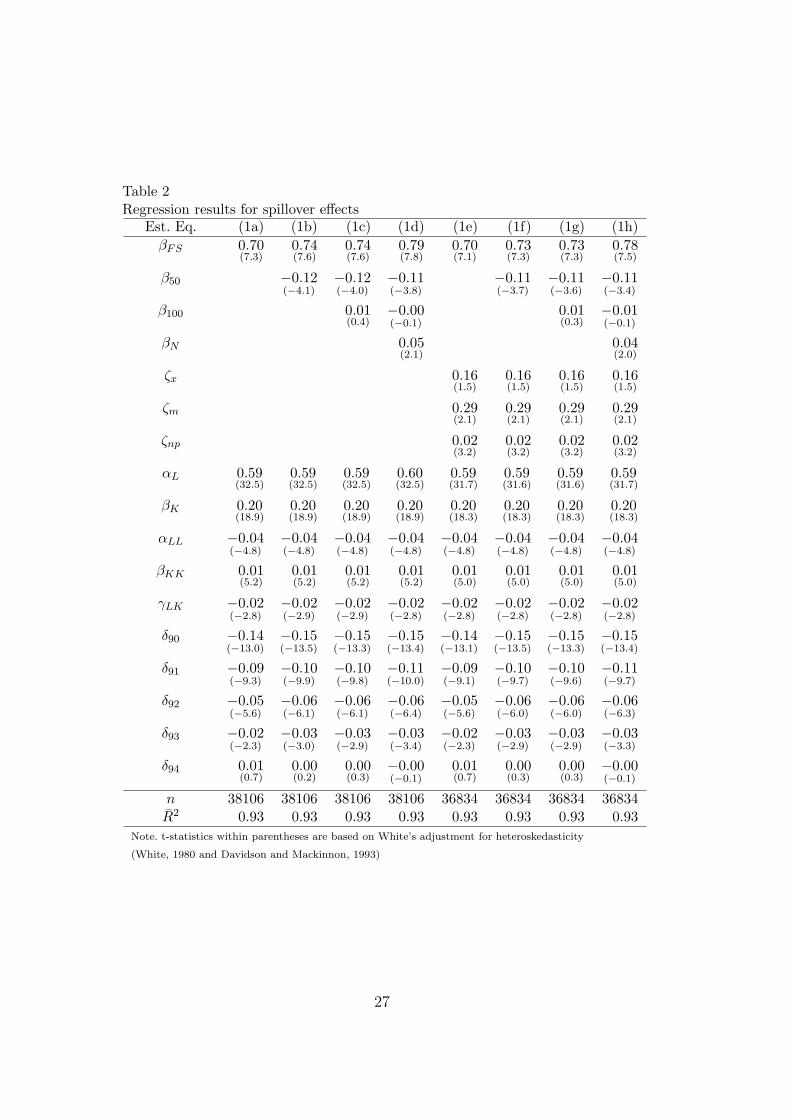
Table 2Regression results for spillover effects

Est. Eq. (1a) (1b) (1c) (1d) (1e) (1f) (1g) (1h)βFS 0.70

(7.3)0.74(7.6)

0.74(7.6)

0.79(7.8)

0.70(7.1)

0.73(7.3)

0.73(7.3)

0.78(7.5)

β50 −0.12(−4.1)

−0.12(−4.0)

−0.11(−3.8)

−0.11(−3.7)

−0.11(−3.6)

−0.11(−3.4)

β100 0.01(0.4)

−0.00(−0.1)

0.01(0.3)

−0.01(−0.1)

βN 0.05(2.1)

0.04(2.0)

ζx 0.16(1.5)

0.16(1.5)

0.16(1.5)

0.16(1.5)

ζm 0.29(2.1)

0.29(2.1)

0.29(2.1)

0.29(2.1)

ζnp 0.02(3.2)

0.02(3.2)

0.02(3.2)

0.02(3.2)

αL 0.59(32.5)

0.59(32.5)

0.59(32.5)

0.60(32.5)

0.59(31.7)

0.59(31.6)

0.59(31.6)

0.59(31.7)

βK 0.20(18.9)

0.20(18.9)

0.20(18.9)

0.20(18.9)

0.20(18.3)

0.20(18.3)

0.20(18.3)

0.20(18.3)

αLL −0.04(−4.8)

−0.04(−4.8)

−0.04(−4.8)

−0.04(−4.8)

−0.04(−4.8)

−0.04(−4.8)

−0.04(−4.8)

−0.04(−4.8)

βKK 0.01(5.2)

0.01(5.2)

0.01(5.2)

0.01(5.2)

0.01(5.0)

0.01(5.0)

0.01(5.0)

0.01(5.0)

γLK −0.02(−2.8)

−0.02(−2.9)

−0.02(−2.9)

−0.02(−2.8)

−0.02(−2.8)

−0.02(−2.8)

−0.02(−2.8)

−0.02(−2.8)

δ90 −0.14(−13.0)

−0.15(−13.5)

−0.15(−13.3)

−0.15(−13.4)

−0.14(−13.1)

−0.15(−13.5)

−0.15(−13.3)

−0.15(−13.4)

δ91 −0.09(−9.3)

−0.10(−9.9)

−0.10(−9.8)

−0.11(−10.0)

−0.09(−9.1)

−0.10(−9.7)

−0.10(−9.6)

−0.11(−9.7)

δ92 −0.05(−5.6)

−0.06(−6.1)

−0.06(−6.1)

−0.06(−6.4)

−0.05(−5.6)

−0.06(−6.0)

−0.06(−6.0)

−0.06(−6.3)

δ93 −0.02(−2.3)

−0.03(−3.0)

−0.03(−2.9)

−0.03(−3.4)

−0.02(−2.3)

−0.03(−2.9)

−0.03(−2.9)

−0.03(−3.3)

δ94 0.01(0.7)

0.00(0.2)

0.00(0.3)

−0.00(−0.1)

0.01(0.7)

0.00(0.3)

0.00(0.3)

−0.00(−0.1)

n 38106 38106 38106 38106 36834 36834 36834 36834R2 0.93 0.93 0.93 0.93 0.93 0.93 0.93 0.93

Note. t-statistics within parentheses are based on White’s adjustment for heteroskedasticity

(White, 1980 and Davidson and Mackinnon, 1993)

27

Table 3Regression results for spillover effects and technological gapsClassification average wage gap average labor productivity gap

Eq. (1a) (1b) (1a) (1b)Group LW HW LW HW LP HP LP HPβFS 0.97

(6.9)0.54(3.8)

0.94(6.7)

0.60(4.2)

1.03(7.1)

0.52(3.7)

1.00(6.8)

0.57(4.1)

β50 −0.08(−1.5)

−0.09(−2.6)

−0.06(−1.3)

−0.09(−2.1)

αL 0.59(19.5)

0.59(25.1)

0.59(19.4)

0.59(25.1)

0.59(20.1)

0.59(25.0)

0.59(20.0)

0.59(25.0)

βK 0.23(11.0)

0.19(15.3)

0.23(11.1)

0.19(15.3)

0.23(11.7)

0.19(14.7)

0.23(11.8)

0.19(14.7)

αLL −0.02(−1.8)

−0.04(−4.4)

−0.02(−1.7)

−0.04(−4.4)

−0.03(−2.2)

−0.04(−4.1)

−0.03(−2.2)

−0.04(−4.1)

βKK 0.01(3.0)

0.01(4.2)

0.01(3.1)

0.01(4.2)

0.01(3.2)

0.01(4.1)

0.01(3.2)

0.01(4.1)

γLK −0.03(−2.4)

−0.02(−2.0)

−0.03(−2.5)

−0.02(−2.0)

−0.03(−2.5)

−0.02(−1.9)

−0.03(−2.5)

−0.02(−1.9)

δ90 −0.06(−2.7)

−0.18(−13.7)

−0.07(−3.0)

−0.18(−13.9)

−0.06(−3.1)

−0.18(−13.5)

−0.07(−3.4)

−0.18(−13.6)

δ91 −0.05(−2.5)

−0.12(−9.4)

−0.05(−2.8)

−0.12(−9.7)

−0.05(−3.2)

−0.12(−9.1)

−0.06(−3.4)

−0.12(−9.3)

δ92 −0.04(−2.4)

−0.06(−5.3)

−0.04(−2.4)

−0.07(−5.7)

−0.04(−2.3)

−0.06(−5.5)

−0.04(−2.4)

−0.07(−5.7)

δ93 −0.01(−0.8)

−0.03(−2.6)

−0.01(−0.6)

−0.04(−3.2)

−0.02(−1.2)

−0.03(−2.4)

−0.02(−1.1)

−0.03(−2.9)

δ94 −0.01(−0.4)

0.01(1.0)

−0.01(−0.4)

0.01(0.5)

−0.01(−0.9)

0.01(1.2)

−0.01(−0.9)

0.01(0.8)

n 11171 26935 11171 26935 12124 25982 12124 25982R2 0.93 0.93 0.93 0.93 0.93 0.94 0.93 0.94

Wald test for H0 : βLFS = βH

FS , H1 : βLFS 6= βH

FS

p-value 0.03 0.09 0.01 0.03Note. t-statistics within parentheses are based on White’s adjustment for heteroskedasticity

(White, 1980 and Davidson and Mackinnon, 1993)

28

Table 4Regression results for spillovers and plant size and capital intensityClassification plant size plant capital intensity

Eq. (1a) (1b) (1a) (1b)Group LS HS LS HS LK HK LK HKβFS 0.73

(7.0)0.66(2.8)

0.76(7.2)

0.69(2.9)

0.76(7.3)

0.55(2.5)

0.80(7.6)

0.58(2.6)

β50 −0.10(−3.3)

−0.14(−2.1)

−0.11(−3.6)

−0.12(−1.8)

αL 0.65(25.7)

0.54(15.3)

0.65(25.7)

0.54(15.3)

0.60(23.9)

0.60(21.4)

0.60(23.8)

0.60(21.4)

βK 0.22(15.3)

0.18(9.3)

0.22(15.3)

0.18(9.3)

0.21(14.2)

0.19(12.1)

0.21(14.3)

0.19(12.1)

αLL −0.01(−1.3)

−0.04(−2.7)

−0.01(−1.3)

−0.04(−2.6)

−0.04(−4.1)

−0.03(−2.4)

−0.04(−4.1)

−0.03(−2.4)

βKK 0.02(6.1)

−0.00(−0.1)

0.02(6.2)

−0.00(−0.1)

0.01(4.7)

0.01(0.9)

0.01(4.8)

0.01(0.9)

γLK −0.02(−2.6)

0.01(0.6)

−0.02(−2.6)

0.01(0.6)

−0.02(−2.3)

−0.01(−0.9)

−0.02(−2.3)

−0.01(−0.9)

δ90 −0.17(−14.8)

0.01(0.2)

−0.18(−15.2)

−0.00(−0.2)

−0.15(−12.7)

−0.11(−4.5)

−0.16(−13.2)

−0.12(−4.8)

δ91 −0.12(−11.1)

0.01(0.5)

−0.13(−11.5)

0.00(0.0)

−0.12(−10.3)

−0.04(−1.7)

−0.12(−10.8)

−0.05(−2.0)

δ92 −0.07(−6.5)

−0.00(−0.1)

−0.07(−6.9)

−0.01(−0.4)

−0.08(−7.6)

0.02(1.0)

−0.08(−8.0)

0.02(0.7)

δ93 −0.03(−2.8)

0.01(0.4)

−0.03(−3.4)

0.00(0.1)

−0.02(−2.3)

−0.02(−0.8)

−0.03(−2.9)

−0.02(−1.1)

δ94 0.00(0.2)

0.02(1.1)

−0.00(−0.1)

0.01(0.8)

0.01(0.7)

0.01(0.3)

0.00(0.3)

0.00(0.1)

n 29153 8953 29153 8953 28370 9736 28370 9736R2 0.89 0.93 0.89 0.93 0.93 0.92 0.93 0.92

Wald test for H0 : βLFS = βH

FS , H1 : βLFS 6= βH

FS

p-value 0.78 0.78 0.39 0.37Note. t-statistics within parentheses are based on White’s adjustment for heteroskedasticity

(White, 1980 and Davidson and Mackinnon, 1993)

29

Table 5Regression results for spillovers and human development and R&D activityClassification human development research and development

Eq. (1a) (1b) (1a) (1b)Group LT HT LT HT LR HR LR HRβFS 0.64

(6.3)1.07(3.5)

0.68(6.6)

1.09(3.6)

0.63(6.3)

1.32(3.9)

0.67(6.7)

1.28(3.8)

β50 −0.12(−3.9)

−0.09(−1.0)

−0.14(−4.8)

0.12(1.3)

αL 0.60(29.2)

0.56(12.2)

0.60(29.2)

0.56(12.2)

0.59(30.0)

0.60(10.1)

0.58(29.9)

0.60(10.2)

βK 0.22(17.3)

0.18(8.1)

0.22(17.3)

0.18(8.1)

0.20(17.0)

0.19(7.2)

0.20(17.1)

0.19(7.2)

αLL −0.04(−4.8)

−0.01(−0.7)

−0.04(−4.8)

−0.01(−0.7)

−0.04(−5.3)

0.01(0.4)

−0.04(−5.2)

0.01(0.3)

βKK 0.01(5.5)

0.00(0.1)

0.01(5.5)

0.00(0.1)

0.01(5.2)

0.00(0.0)

0.01(5.3)

0.00(0.0)

γLK −0.02(−2.1)

−0.03(−1.5)

−0.02(−2.1)

−0.03(−1.5)

−0.02(−2.9)

−0.01(−0.3)

−0.02(−3.0)

−0.01(−0.3)

δ90 −0.15(−12.9)

−0.11(−3.1)

−0.15(−13.4)

−0.12(−3.2)

−0.15(−13.2)

−0.09(−2.1)

−0.16(−13.8)

−0.08(−1.9)

δ91 −0.10(−9.8)

−0.03(−0.9)

−0.11(−10.4)

−0.04(−1.1)

−0.11(−10.1)

0.00(0.1)

−0.11(−10.8)

0.01(0.3)

δ92 −0.06(−6.1)

−0.00(−0.1)

−0.06(−6.5)

−0.01(−0.2)

−0.06(−6.2)

0.01(0.4)

−0.07(−6.8)

0.02(0.5)

δ93 −0.02(−2.5)

−0.01(−0.3)

−0.03(−3.1)

−0.01(−0.4)

−0.03(−2.9)

0.03(0.9)

−0.03(−3.7)

0.04(1.1)

δ94 0.01(0.7)

0.00(0.1)

0.00(0.2)

0.00(0.0)

0.00(0.1)

0.06(1.8)

−0.00(−0.5)

0.06(1.9)

n 34092 4014 34092 4014 34814 3292 34814 3292R2 0.93 0.92 0.93 0.92 0.93 0.92 0.93 0.92

Wald test for H0 : βLFS = βH

FS , H1 : βLFS 6= βH

FS

p-value 0.19 0.21 0.05 0.08Note. t-statistics within parentheses are based on White’s adjustment for heteroskedasticity

(White, 1980 and Davidson and Mackinnon, 1993)

30