Robotics 2

Prof. Alessandro De Luca

Impedance Control

Impedance control

n imposes a desired dynamic behavior to the interaction between robot end-effector and environment

n the desired performance is specified through a generalized dynamic impedance, namely a complete set of mass-spring-damper equations (typically chosen as linear and decoupled, but also nonlinear)

n a model describing how reaction forces are generated in association with environment deformation is not explicitly required

n suited for tasks in which contact forces should be “kept small”, while their accurate regulation is not mandatory

n since a control loop based on force error is missing, contact forces are only indirectly assigned by controlling position

n the choice of a specific stiffness in the impedance model along a Cartesian direction results in a trade-off between contact forces and position accuracy in that direction

Robotics 2 2

with

generalized forces performing work on �̇�

𝑀 𝑞 �̈� + 𝑆 𝑞, �̇� �̇� + 𝑔 𝑞 = 𝑢 + 𝐽-. 𝑞 𝐹-𝐹- = 𝑇-1. 𝜙 𝐹

Dynamic model of a robot in contactgeneralized

Cartesian force

Robotics 2 3

𝑀 𝑞 �̈� + 𝑆 𝑞, �̇� �̇� + 𝑔 𝑞 = 𝑢 + 𝐽. 𝑞 𝐹𝑞 ∈ ℝ5

forces

torques

performing work on

“geometric”Jacobian

angular velocity derivative ofEuler angles

“analytic”Jacobian

𝐹 = 𝑓𝑚 ∈ ℝ8

linear velocity

𝑉 = 𝑣𝜔 = 𝐽 𝑞 �̇� ≠ �̇� =

�̇��̇� = 𝐽-(𝑞)�̇�

direct kinematics

𝐽- 𝑞 =𝜕𝑓(𝑞)𝜕𝑞 = 𝑇- 𝜙 𝐽(𝑞) �̇� = 𝑇- 𝜙 𝑉

Dynamic model in Cartesian coordinates

... and the usual structural properties§ 𝑀A > 0, if 𝐽- is non-singular

§ �̇�A − 2𝑆A is skew-symmetric, if �̇� − 2𝑆 satisfies the same property

§ the Cartesian dynamic model of the robot can be linearly parameterized in terms of a set of dynamic coefficients

Robotics 2 4

𝑀A 𝑞 �̈� + 𝑆A 𝑞, �̇� �̇� + 𝑔A 𝑞 = 𝐽-1. 𝑞 𝑢 + 𝐹-with𝑀A 𝑞 = 𝐽-1.(𝑞)𝑀(𝑞)𝐽-1F(𝑞)𝑆A 𝑞, �̇� = 𝐽-1. 𝑞 𝑆 𝑞, �̇� 𝐽-1F 𝑞 −𝑀A(𝑞) ̇𝐽-(𝑞)𝐽-1F(𝑞)𝑔A 𝑞 = 𝐽-1.(𝑞)𝑔(𝑞)

assuming𝑛 = 𝑚

Design of the control law

1. feedback linearization in the Cartesian space (with force measure)

2. imposition of a dynamic impedance model

designed in two steps:

closed-loop system

is realized by choosing

most of the timesit is “decoupled”

(diagonal matrices)

Note: 𝑥H(𝑡) is the desired motion, which typically “slightly penetrates” inside the compliant environment (inducing contact forces)...

Robotics 2 5

𝑢 = 𝐽-.(𝑞) 𝑀A 𝑞 𝑎 + 𝑆A 𝑞, �̇� �̇� + 𝑔A 𝑞 − 𝐹-

𝑀8 �̈� − �̈�H + 𝐷8 �̇� − �̇�H + 𝐾8 𝑥 − 𝑥H = 𝐹-

desired (apparent)inertia (> 0)

desireddamping (≥ 0)

desiredstiffness (> 0)

external forcesfrom the environment

�̈� = 𝑎

𝑎 = �̈�H +𝑀81F 𝐷8 �̇�H − �̇� + 𝐾8 𝑥H − 𝑥 + 𝐹-

Examples of desired reference 𝑥𝑑in impedance/compliance control

the desired motion 𝒙𝒅(𝒕) is slightly insidethe environment (keeping thus contact)

Robotics 2 6

𝒙𝒅(𝒕)𝒙𝒆

robot in grinding task robot writing on a surface

𝒙𝒅(𝒕)

𝑀8 �̈� − �̈�H + 𝐷8 �̇� − �̇�H + 𝐾8 𝑥 − 𝑥H = 𝐹-

Examples of desired reference 𝑥𝑑in impedance/compliance control

Robotics 2 7

constant desired pose 𝒙𝒅 is the free Cartesian rest position in a human-robot interaction task

𝒙𝒅

KUKA iiwa robot with human operator KUKA LWR robot in pHRI (collaboration)

𝒙𝒅

𝑀8 �̈� − �̈�H + 𝐷8 �̇� − �̇�H + 𝐾8 𝑥 − 𝑥H = 𝐹-

Control law in joint coordinates

matrix weighting the measured contact forces

§ while the control design is based on dynamic analysis and desired (impedance) behavior described in the Cartesian space, the final control implementation is always at the robot joint level

§ the following identity holds for the term involving contact forces

which eliminates from the control law also the appearance of the last remaining Cartesian quantity (the Cartesian inertia matrix)

substituting and simplifying…

Robotics 2 8

𝑢 = 𝑀 𝑞 𝐽-1F(𝑞)S�̈�H − ̇𝐽- 𝑞 �̇� +𝑀81F }𝐷8 �̇�H − �̇� + 𝐾8 𝑥H − 𝑥+ 𝑆 𝑞, �̇� �̇� + 𝑔 𝑞 + 𝐽-.(𝑞) 𝑀A 𝑞 𝑀81F − 𝐼 𝐹-

𝐽-. 𝑞 𝑀A 𝑞 𝑀81F − 𝐼 𝐹- = 𝑀 𝑞 𝐽-1F(𝑞)𝑀81F − 𝐽-. 𝑞 𝐹-

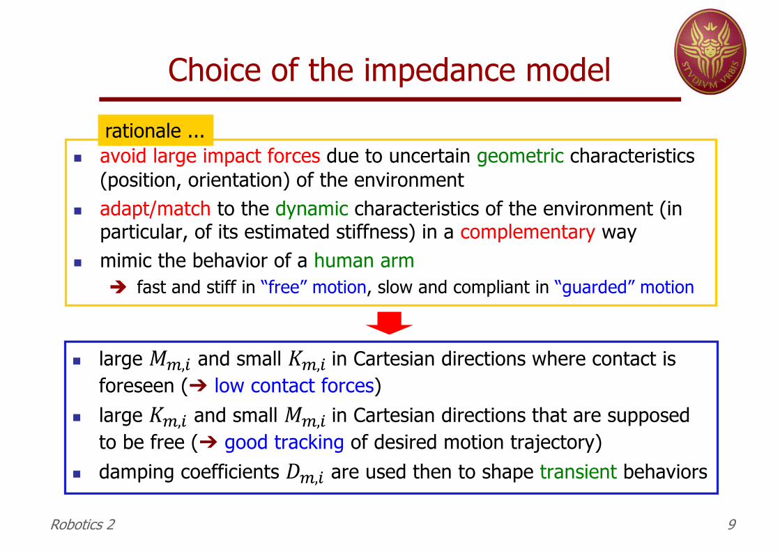
Choice of the impedance model

n avoid large impact forces due to uncertain geometric characteristics (position, orientation) of the environment

n adapt/match to the dynamic characteristics of the environment (in particular, of its estimated stiffness) in a complementary way

n mimic the behavior of a human armè fast and stiff in “free” motion, slow and compliant in “guarded” motion

n large 𝑀8,V and small 𝐾8,V in Cartesian directions where contact is foreseen (➔ low contact forces)

n large 𝐾8,V and small 𝑀8,V in Cartesian directions that are supposed to be free (➔ good tracking of desired motion trajectory)

n damping coefficients 𝐷8,V are used then to shape transient behaviors

rationale ...

Robotics 2 9

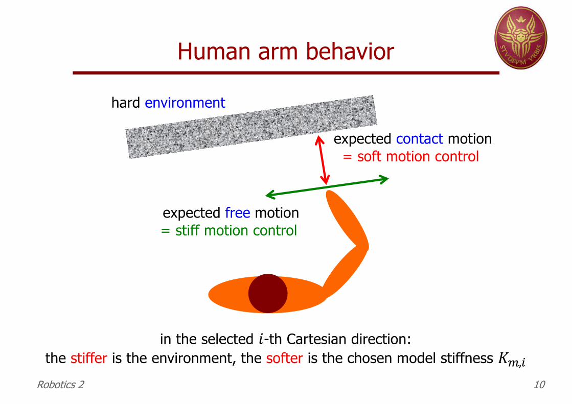
Human arm behavior

Robotics 2 10

hard environment

expected free motion= stiff motion control

expected contact motion= soft motion control

in the selected 𝑖-th Cartesian direction:the stiffer is the environment, the softer is the chosen model stiffness 𝐾8,V

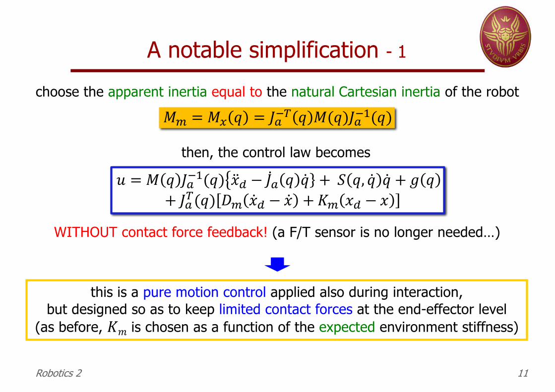
A notable simplification - 1

choose the apparent inertia equal to the natural Cartesian inertia of the robot

this is a pure motion control applied also during interaction,but designed so as to keep limited contact forces at the end-effector level

(as before, 𝐾𝑚 is chosen as a function of the expected environment stiffness)

Robotics 2 11

then, the control law becomes

WITHOUT contact force feedback! (a F/T sensor is no longer needed…)

𝑢 = 𝑀 𝑞 𝐽-1F(𝑞)S�̈�H − ̇𝐽- 𝑞 }�̇� + 𝑆 𝑞, �̇� �̇� + 𝑔 𝑞+ 𝐽-.(𝑞) 𝐷8 �̇�H − �̇� + 𝐾8 𝑥H − 𝑥

𝑀8 = 𝑀A 𝑞 = 𝐽-1. 𝑞 𝑀(𝑞)𝐽-1F(𝑞)

A notable simplification - 2

technical issue: if the impedance model (now, nonlinear) is still supposed to represent a real mechanical system, then in correspondence to a desirednon-constant inertia (𝑀A(𝑞)) there should be Coriolis and centrifugal terms...

§ guarantee of asymptotic convergence to zero tracking error (on 𝑥𝑑(𝑡))when 𝐹- = 0 (no contact situation) ⇒ Lyapunov + skew-symmetry of �̇�A − 2𝑆A

§ further simplifications when 𝑥𝑑 is constant

Robotics 2 12

nonlinear impedance model (“only” gravity terms disappear)

𝑀A(𝑞) �̈� − �̈�H + 𝑆A 𝑞, �̇� + 𝐷8 �̇� − �̇�H + 𝐾8 𝑥 − 𝑥H = 𝐹-

redoing computations, the control law becomes

which is indeed slightly more complex, but has the following advantages:

𝑢 = 𝑀 𝑞 𝐽-1F(𝑞)S�̈�H − ̇𝐽- 𝑞 }𝐽-1F 𝑞 �̇�H + 𝑆 𝑞, �̇� 𝐽-1F(𝑞)�̇�H + 𝑔 𝑞+ 𝐽-.(𝑞) 𝐷8 �̇�H − �̇� + 𝐾8 𝑥H − 𝑥

Cartesian regulation revisited (without contact, 𝐹- = 0)

when 𝑥𝑑 is constant (�̇�H = 0, �̈�H = 0), from the previous expression we get the control law

Cartesian PD control with gravity cancellation…

when 𝐹- = 0 (absence of contact), we know already that this control law ensures asymptotic stability of 𝑥H, provided 𝐽-(𝑞) has full rank

proof(alternative) Lyapunov candidate

using skew-symmetry of �̇�A − 2𝑆A and 𝑔A = 𝐽-1.𝑔

(★)

Robotics 2 13

𝑢 = 𝑔 𝑞 + 𝐽-. 𝑞 𝐾8 𝑥H − 𝑥 −𝐷8�̇�

𝑉F =12 �̇�

.𝑀A 𝑞 �̇� +12 𝑥H − 𝑥 .𝐾8 𝑥H − 𝑥

�̇�F = �̇�.𝑀A 𝑞 �̈� +12�̇�.�̇�A 𝑞 �̇� − �̇�.𝐾8 𝑥H − 𝑥 = ⋯ = −�̇�.𝐷8�̇� ≤ 0

Cartesian stiffness control(with contact, 𝐹- ≠ 0)

when 𝐹- ≠ 0, convergence to 𝑥H is not assured (it may not even be a closed-loop equilibrium…)

§ for analysis, assume an elastic contact model for the environment

𝐹- = 𝐾\(𝑥\ − 𝑥) with stiffness 𝐾\ ≥ 0 and rest position 𝑥\§ closed-loop system behavior

Lyapunov candidate

Robotics 2 14

𝑉] =12 �̇�

.𝑀A 𝑞 �̇� +12 𝑥H − 𝑥 .𝐾8 𝑥H − 𝑥 +

12 𝑥\ − 𝑥 .𝐾\ 𝑥\ − 𝑥

= 𝑉F +12𝑥\ − 𝑥 .𝐾\ 𝑥\ − 𝑥

�̇�] = �̇�.𝑀A 𝑞 �̈� +12�̇�.�̇�A 𝑞 �̇� − �̇�.𝐾8 𝑥H − 𝑥 − �̇�.𝐾\ 𝑥\ − 𝑥

= ⋯ = −�̇�.𝐷8�̇� + �̇�.(𝐹- − 𝐾\ 𝑥\ − 𝑥 ) = −�̇�.𝐷8�̇� ≤ 0

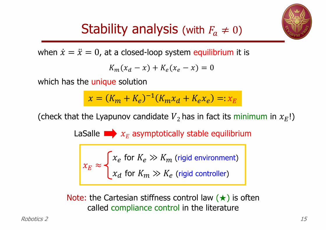
Stability analysis (with 𝐹- ≠ 0)

when �̇� = �̈� = 0, at a closed-loop system equilibrium it is

𝐾8(𝑥H − 𝑥) + 𝐾\(𝑥\ − 𝑥) = 0

𝑥 = 𝐾8 +𝐾\ 1F 𝐾8𝑥H + 𝐾\𝑥\ =: 𝑥_

𝑥\ for 𝐾\ ≫ 𝐾8 (rigid environment)

𝑥H for 𝐾8 ≫ 𝐾\ (rigid controller)𝑥_ ≈

(check that the Lyapunov candidate 𝑉2 has in fact its minimum in 𝑥_!)

Note: the Cartesian stiffness control law (★) is oftencalled compliance control in the literature

Robotics 2 15

LaSalle 𝑥𝐸 asymptotically stable equilibrium

which has the unique solution

Active equivalent of RCC device§ displacements from the desired position 𝑥H are small, namely

§ 𝑔(𝑞) = 0 (gravity is compensated/cancelled, e.g., mechanically)§ 𝐷8 = 0

(𝑥H − 𝑥) ≈ 𝐽-(𝑞H − 𝑞)IF

constant Cartesian-level stiffness 𝐾8corresponds to

variable joint-level stiffness 𝐾(𝑞)

is the ‘‘active’’ counterpart of a Remote Center of Compliance (RCC) device

Robotics 2 16

THEN 𝑢 = 𝐽-. 𝑞 𝐾8 𝐽- 𝑞H − 𝑞 = 𝐾(𝑞)(𝑞H − 𝑞)

∆𝑥 𝐾8 𝐹

∆𝑞

𝐽-(𝑞) 𝐽-.(𝑞)

𝑢𝐾(𝑞)

𝐶(𝑥)∆𝑥 𝐹

𝐽-1F(𝑞) 𝐽-1.(𝑞)

∆𝑞 𝑢𝐶8(and vice versa on compliance)

Admittance control

Robotics 2 17

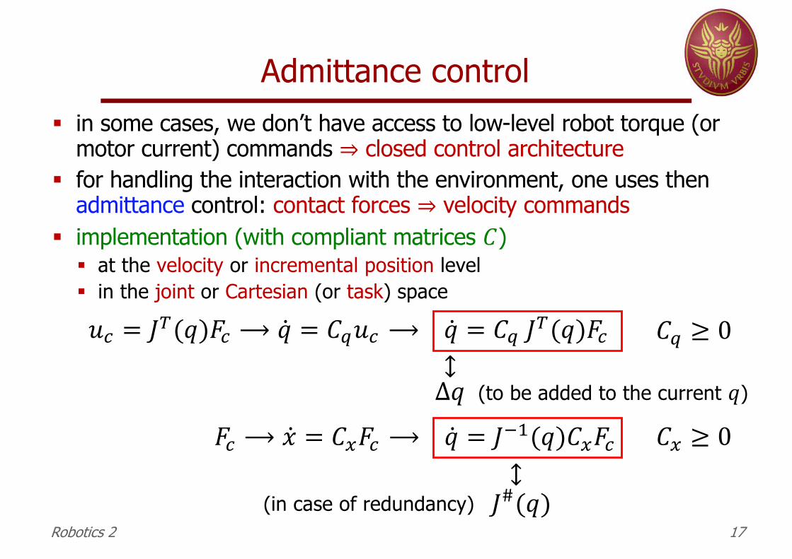
§ in some cases, we don’t have access to low-level robot torque (or motor current) commands ⇒ closed control architecture

§ for handling the interaction with the environment, one uses then admittance control: contact forces ⇒ velocity commands

§ implementation (with compliant matrices 𝐶)§ at the velocity or incremental position level§ in the joint or Cartesian (or task) space

𝐹e ⟶ �̇� = 𝐶A𝐹e ⟶ �̇� = 𝐽1F(𝑞)𝐶A𝐹e

𝑢e = 𝐽.(𝑞)𝐹e ⟶ �̇� = 𝐶g𝑢e ⟶ �̇� = 𝐶g 𝐽.(𝑞)𝐹e↕∆𝑞 (to be added to the current 𝑞)

↕𝐽#(𝑞)(in case of redundancy)

𝐶g ≥ 0

𝐶A ≥ 0