Hydraulics Prof. Dr. Arup Kumar Sarma

Department of Civil Engineering Indian Institute of Technology, Guwahati

Module No. # 06

Canal Design Lecture No. # 02

Design of Alluval Channel

Then, because the erosion question is not coming, but here in the Design of unlined

canal, this erosion is coming very much. And of course, in case of non-alluvial channel,

where erosion is not that much significant, it can be significant or it becomes significant

when the velocity exceed a particular limit, and that we call as a maximum permissible

velocity. So, in non-alluvial channel, our design principle is that our velocity should not

exceed a maximum permissible velocity and then of course, if it carries some sediment,

which is not a regular problem of non-alluvial channel, but still if it carries some

sediment, in that case, the velocity also must exceed a very minimum velocity, which

will not allow sedimentation, if that water carries sediment or if sediment let in water

come through the channel.

That was a the discussion about non-alluvial channel and today we shall be discussing on

Alluvial channel and of course, we started discussion on Alluvial channel earlier and on

Alluvial channel, our main criteria the design criteria is the concept of Critical velocity,

that we did discuss in last class.

(Refer Slide Time: 02:08)

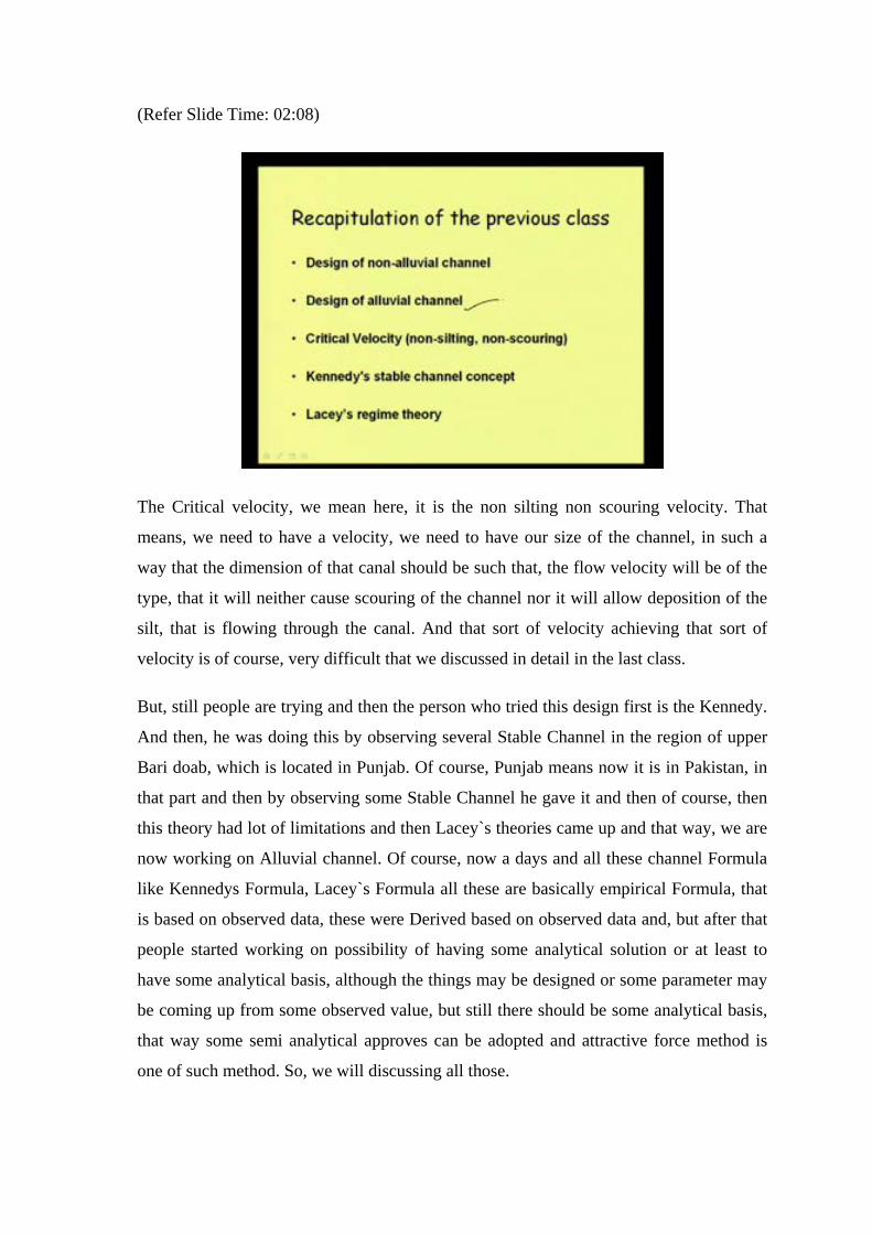
The Critical velocity, we mean here, it is the non silting non scouring velocity. That

means, we need to have a velocity, we need to have our size of the channel, in such a

way that the dimension of that canal should be such that, the flow velocity will be of the

type, that it will neither cause scouring of the channel nor it will allow deposition of the

silt, that is flowing through the canal. And that sort of velocity achieving that sort of

velocity is of course, very difficult that we discussed in detail in the last class.

But, still people are trying and then the person who tried this design first is the Kennedy.

And then, he was doing this by observing several Stable Channel in the region of upper

Bari doab, which is located in Punjab. Of course, Punjab means now it is in Pakistan, in

that part and then by observing some Stable Channel he gave it and then of course, then

this theory had lot of limitations and then Lacey`s theories came up and that way, we are

now working on Alluvial channel. Of course, now a days and all these channel Formula

like Kennedys Formula, Lacey`s Formula all these are basically empirical Formula, that

is based on observed data, these were Derived based on observed data and, but after that

people started working on possibility of having some analytical solution or at least to

have some analytical basis, although the things may be designed or some parameter may

be coming up from some observed value, but still there should be some analytical basis,

that way some semi analytical approves can be adopted and attractive force method is

one of such method. So, we will discussing all those.

(Refer Slide Time: 04:23)

Let us just start with some of those important issues of Kennedys Silt Theory, that we did

discuss in the last class, but still we will be just starting from that aspect. So, you can

concentrate in the slide, because we will be showing the Formula here basically, that it

gave this theory, he gave this theory based on his observation of several stable reach. I

am under lining this one, several stable reach of upper Bari Doab canal system of Punjab

and now in Pakistan. Then he measured the Flow Velocity actually after getting those

stable reach, he measured the Flow Velocity and he named this as V 0.

So, this V 0 he measured and of course, he considered that this V 0 velocity will be

having a relationship with that Depth of flow. That means, if the Flow Velocity and

Depth, we observe, then we find that the stable remain and the channel remain stable for

a velocity and at that velocity, if the Depth is having a particular value. So, that way he

tried to relate this Depth and the velocity, and at that point he considered that the width

of the channel has nothing to do with this relation, and then relating this V 0 and the

Depth D, he plotted this data in a curve and then after plotting these things, he derived

this particular relation, that is V 0, velocity V 0 is equal to 0.55.

Then D means Depth to the power 0.64, means suppose, if we plot the V 0 in this

direction, I am just giving one example, V 0 for all those stable channel, suppose several

stable channels are there in the upper Bari Doab canal portion, then he observed, then he

found that some D 0, he D he is measuring Depth and then at the same time, for that

particular portion what is the Flow Velocity, that he is observing. And for several years,

that he found that for several years, this particulars channel is stable. And that is why he

took those channel portion and then say putting this V 0 and this D say he is getting a

curve like this. Exactly what sort of curve he got that is not a question here but suppose

he got several points and say for example I am giving suppose the points can be plotted

like this and the equation of this particular curve may give us one relation or a equation.

So, that equation is say this one V 0 is equal to 0.5 D to the power 0.64 where this V 0 is

in meter per second, this V 0 is in meter per second and D is in meter. So, this was the

popular and famous Formula of Kennedy and then he as I said that, he did not consider

the effect of, I mean this width of channel on Critical velocity and then in fact, to

introduce the effect of silt size, here as we can observe in this Formula, this velocity, he

is saying that this velocity is the Critical velocity, where no erosion, no deposition will

take place. And this Depth is only the parameter on which he is deriving this velocity,

but from our general concept, we know one thing that, at a particular velocity whether

there will be erosion or whether there will be deposition, that will definitely depend on

the silt size. If the bed material, that is consisting of very fine silt, then at a very low

velocity also, this can be eroded, if it is suppose a larger size silt, then it may not be

eroded.

So, that way, the silt will definitely have some influence on the entire relationship and

when he initially observed, he did not consider those effect of silt, because the very

reason is there, he was observing this value only in the region that is the upper Bari

Doab, the canal system, and for that canal system the sediment size or the silt size of the

canal are same, I mean identical in all the channel reach, he considered these were same.

So, what he observed, then he got the same value, he got that this relation is valid, but if

we put a different kind of silt, then definitely the relation what we obtain will not be

valid and that he could realize later when this formula was attempted applying in

different area having different silt grade, by silt grade we are meaning silt size, what is

the proportion of silt size in a particular silt sample and what is the average size? we call

it as a D 50 average size.

So, that way this effect came later and so to introduce the effect of silt size, later he

introduced a factor m and this factor is called Critical velocity Ratio, he named this as

Critical Velocity Ratio.

(Refer Slide Time: 09:58)

So, what is this Ratio is Critical velocity Ratio? That if we see that this m was

introduced, which is called Critical velocity Ratio well. So, m means it is V by V 0.

Now, what this V 0? V 0 is the velocity or Critical velocity, we can write it as Critical

velocity of upper Bari Doab channel region, Critical velocity of upper Bari Doab canal

region canal system upper Bari Doab canal system. And, then this V is the Critical

velocity. Somewhere else means, the place under consideration. By this what we mean

that if we know the Critical velocity for the upper Bari Doab canal region, then we can

find the Critical velocity in other place or indirectly, if we know the m value for a

particular region or a particular type of sediment, then we can find the Critical velocity

for that particular place. So, when m is greater than 1, then it is greater than 1 for silt

coarser than the upper Bari Doab canal region.

So, that means, for suppose upper Bari Doab canal region, we have a V 0 value, then if

the silt size for a different region is, greater than or the size is larger than the upper Bari

Doab channel region, then definitely the Critical velocity will be larger. It will be say

erosion, that means, the larger size larger velocity will be required for eroding the

channel. So, that way it will be larger and that is why this m value will be greater than 1.

And if your silt is finer, then the upper Bari Doab canal region, then this m value will be

smaller and so, then people are investigating and different other followers are walking on

that line and they have given some value for m also, for different part of the country and

then definitely for using this equation, we cannot, we should not use directly in a

particular region. Once we are sure about this m value, say this equation was developed

in the region of Punjab, now if we want to which is on the west western part of our

country, and then if we try to apply that equation in the suppose eastern part of the

country. Then we should conduct some experiment then only we will be knowing that

this will be the m value for this particular region and then only we should apply this

formula of course, this Kennedys Formula has some of the limitation.

(Refer Slide Time: 13:07)

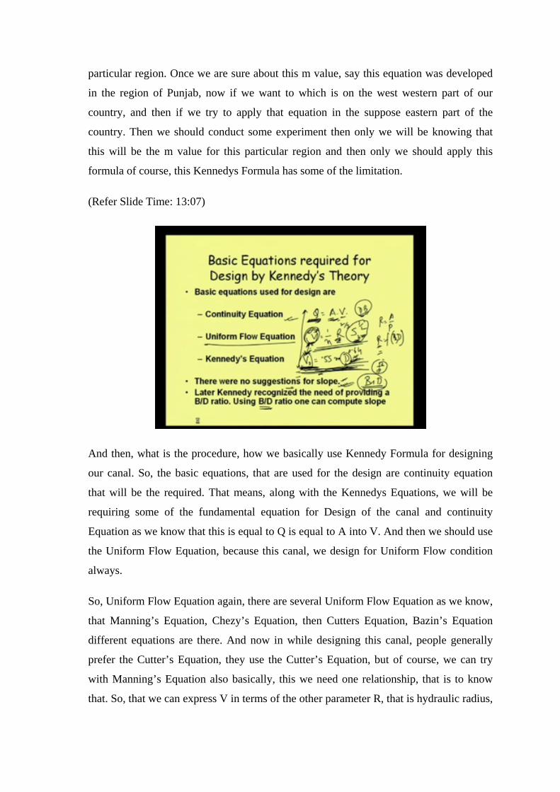
And then, what is the procedure, how we basically use Kennedy Formula for designing

our canal. So, the basic equations, that are used for the design are continuity equation

that will be the required. That means, along with the Kennedys Equations, we will be

requiring some of the fundamental equation for Design of the canal and continuity

Equation as we know that this is equal to Q is equal to A into V. And then we should use

the Uniform Flow Equation, because this canal, we design for Uniform Flow condition

always.

So, Uniform Flow Equation again, there are several Uniform Flow Equation as we know,

that Manning’s Equation, Chezy’s Equation, then Cutters Equation, Bazin’s Equation

different equations are there. And now in while designing this canal, people generally

prefer the Cutter’s Equation, they use the Cutter’s Equation, but of course, we can try

with Manning’s Equation also basically, this we need one relationship, that is to know

that. So, that we can express V in terms of the other parameter R, that is hydraulic radius,

roughness parameter, now I am writing as 1 by n and the slope and based on all those

parameter, if I write Manning’s Equation it will be 2 by 3 S to the power half. So, S B n,

R is a R is the Ratio of Area by Perimeter as we all know and that means, R is a function

of what is your B value, what is your y value that means, what is your width and what is

our depth. So, based on that we can express the velocity.

So, this is 1 relation that we know and then of course, our main equation for Design of

the canal, that is the Kennedys Equation, that will be required, that is V 0, as we are

writing this 1 is equal to 0.55 m and D to the power 0.64 and this is in matrix unit that is

the D is in meter, V 0 is in meter per second, but in this entire computational process, for

designing that channel, there is no mention about the slope. That means, if we do it, if we

calculate our size of the canal, here we are not considering the Bed Slope, particularly

when we were using the Kennedys Equation, we are finding that this is the V 0, if we

Assume a Depth D. And then we are calculating the Critical velocity, then once we get

the Critical velocity, we can get the Area of the canal. Then from the Area of the canal,

Area is again a function of B and y, so, y means the depth I am talking about and here of

course, we are using the symbol D. So, in this place also I can write D in place of y.

So, depth, so, depth is already known. So, B we can calculate and then calculating the b,

so, once we get D and B, then using this D and B, we can calculate R, then of course,

Bed Slope will be known to us. So, for that Bed Slope, we can now calculate our

Uniform Flow Velocity V, we can use Cutters Equations also, as it is very lengthy, I am

just writing the Manning Equations here V we can use. Now, So, far our requirement is

concern, that we are considering this is to be Critical velocity, but when we calculate by

using Uniform Flow Formula, after getting B and D from this Continuity Equation and

this Kennedys Equation, we will be getting another Uniform Flow velocity, but if these 2

velocity are not matching, that means, our design is not correct, we are considering

something to be Critical velocity, but in reality, we are getting something else, because

the Flow Velocity, what we are getting by using Uniform Flow Formula is actually the

velocity, what will be getting in the field.

So, it is not matching. That means, the D, what we assume, initially we assume a D

value, rather we took, we take a trial value of D. So, that trial value of D, that we did take

is not correct. So, what we will have to do, we will have to change the D value. That

means, for that D value, we are not arriving into a position that our Uniform Flow

velocity, what we are getting is not matching with the or it is not becoming the critical

velocity. So, that D will not survive proper.

So, we will take another D and then we will again calculate our V 0 and then with that V,

we will be finding area then again we will be getting B and D, that is the Depth and

width and we are again trying what actually we are getting in the field by using the

Uniform Flow formula. So, that trial and error procedure is required here and once we

find that both the V is matching, then we are getting that, I mean, the channel what we

are proposing, the design what we are suggesting for B and D are of course, acceptable.

So, that is what the basic procedure is, but in this formula we are not talking about

anything about the slope in the Kennedys Formula.

And then later and of course, we are calculating the B and D based on this continuity

equation, then later Kennedy, he realized that, no, there is a need of putting some

relationship or some proportion of B also, because when he is equating, when he is trying

to find this Critical velocity with respect to D and at the same time he found that a B by

D ratio can be given. That if this is the D, then this should be the B, that this then only

the channel will become stable. So, based on that, some experimentation were carried out

and so, departments of Punjab area that time also, they conducted experiment and they

gave some B by D Ratio. Now, what is the advantage of having this B by D ratio?

Because, earlier also we could calculate our ultimate size of the channel, because where

which match with this V, that is the Kennedys velocity and the Uniform Flow velocity.

So, that we could do.

But, as it was stated, I have also mentioned, that slope was not considered at that point.

We are considering a slope, which we are getting from the natural terrain, that is from

the topography of the channel, rather topography of the area, we are considering that this

is the slope we can provide, but always their remain a scope of adjusting the slope to

some extent. That is, I was explaining that part earlier also. Let me take some space, say

this is the area and there suppose to carry the water from this point to that point, point A

to point B, we under construct a canal. Now, we can make the canal, suppose we are

starting digging here and then we can make the canal like this or one can feel that no he

will go like this, he will go like this. And then, another may think that we will carry, we

will do some of that, in this case he is cutting this much, depositing this much, in this

case, he is cutting here lot, but no deposition and he is going like that. So, that way there

is a scope of adjusting the slope to some extent and that we cannot achieve when we use,

when we do not use rather B by D Ratio, then we do not have the scope of adjusting the

slope.

And when we use B by D Ratio, then what we can do? We can use this B by D Ratio to

find, once we can find, we are assuming a D. So, now, considering that B by. So, from

that we are getting a V and then from the B by D Ratio, we will be getting a B also. And

using that B, we can directly put it using that B, now we can just try to see that if we

adjust the slope with that B and D value, can we get this velocity. So, we will try

adjusting this, as B and with some adjustment of this as B, we will try that if we can have

this, because once we get this once we assume this D value, that as we have a B by D

ratio. So, both B and D are with us. Now, putting this B by D, we can get this relation

and then we can try to see that whether we can adjust this value or not. Of course, this Q

is our primary requirement, because we are trying to put that much of discharge. So, this

Q is equal A into V we have to be satisfied.

(Refer Slide Time: 22:35)

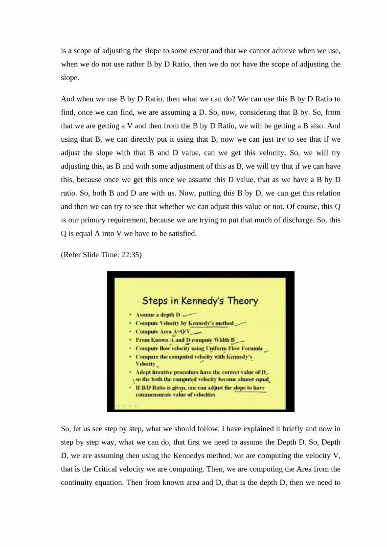
So, let us see step by step, what we should follow. I have explained it briefly and now in

step by step way, what we can do, that first we need to assume the Depth D. So, Depth

D, we are assuming then using the Kennedys method, we are computing the velocity V,

that is the Critical velocity we are computing. Then, we are computing the Area from the

continuity equation. Then from known area and D, that is the depth D, then we need to

compute the width D, that is the bed width D, of course, when we are using this Q and

this our shape can be trapezoidal, shape can be rectangular, anything it can be, that we

will have to decide, again we did discuss about that part also how we decide this slope,

that we will have to do. Then, next step is that Compute Flow Velocity using Uniform

Flow Formula, this Uniform Flow Formula can be Cutters or Manning’s, but basically

Cutters Equation is preferred here.

Then we should compare the computed velocity with Kennedys velocity, computed

velocity means this Uniform Flow Formula what velocity we are getting, then from this

step, we should go for iterative procedure. So, adopt iterative procedure and have that

correct value of D. So, that both the computed velocity by the Kennedy method and by

the Uniform Flow method that become almost equal of course, we can go for almost

equal, exact value may not be matching. So, this is what the procedure is and if B by D

Ratio is given, one can adjust the slope to have commensurate value of velocity.

So, commensurate value of velocity means again, these two velocity should be almost

equal. So, that is what the steps, that we follow in Kennedys theory. After Kennedy’s

theory, the next theory that came is Lacey`s Regime Theory. We just gave the name

earlier in the last class and then we discuss the originally, when it was developed and all

those things. So, we are not going to that part, but his principal is the Regime Channel,

his principal is the Regime Channel and of course, it is similar to having a Critical

velocity, but what he suggesting that for a particular size of the channel, the channel can

be regarded to be in regime condition and naturally, if we allow, what is Regime

condition, the naturally if we allow the water to flow in a channel, then depending on the

Flow Velocity and the size of the channel, it may happen that, if it has the erosion power,

the water will have erosive power if the Flow Velocity is high.

Then, it will start eroding the channel in Alluvial channel I am talking about. So, it will

start eroding the channel. And, just the reverse if we think that, if it is the size of the

channel is very large and the Flow Velocity is very low as such, that means, we are

talking always about all this fact, when we are talking about a particular discharge. So,

for that discharge, if our Flow Velocity is very less, then as it will be carrying some

sediment with it, because it is in a Alluvial channel. So, sediment is a must, I mean,

sediment will have to flow through the water. So, that is why then those sediment will

start depositing in the pair and then so, ultimately what we can see that, if we allow a

channel to run for a long time, it will adjust its own size, the width may increase, the

depth may increase or due to sedimentation width may decrease and depth may decrease.

So, that process will continue and after continuing this process for a very long period, it

will come to a stage, that it will not change its width or depth further and that condition

is referred as Regime condition, that condition is basically referred as Regime condition.

(Refer Slide Time: 27:21)

So, as a definition of Regime condition, we can state like that. Alluvial channel carrying

a certain discharge and that part is very important, that when we are talking that this

channel is in Regime condition, we are always talking about that, it is in a Regime

condition for this particular discharge, that is very important. So, it is carrying a certain

discharge. Alluvial channel carrying a certain discharge undergoes changes in bed width,

depth and slope of course, in when I was saying, I was not mentioning about the slope,

the slope will also get adjusted, when discharge is when the velocity is more, it will be

eroding and slope may that way get increase, when discharge is for that particular

discharge when velocity is less, sedimentation will be there and if the sediments start

from downstream, then discharge slope can reduce of course, if the sedimentation takes

place at the upstream itself, then downstream is so, all sediments are getting deposited at

the upstream then when all sediments are depositing at the upstream and downstream is

getting free of sediment then again that water may start eroding and that way slope can

increases also.

So, that way this change of slope will continue. So, this slope is also getting adjusted and

until an equilibrium is reached. So, finally, it will reach an equilibrium, until an

equilibrium is reached and become a Stable Channel and that Stable Channel is called

the channel is in Regime condition. And for using Lacey’s Theory or before going to

Lacey’s Theory some of the term we should have very clear idea, that is we say that

Lacey’s principle will give us 1 channel, which will be in Regime condition, but what is

Regime condition we have explained, but then we should know what is True regime

condition. So, understanding following terms are important. That is first, we let us see

what we mean by True regime condition, because many a time, we say that this is in

Regime condition, but True regime conditions are very special and of course, we must

know that in practical field, getting a True regime condition is very difficult, but still we

go with that assumption.

Now, for True regime condition, discharge is constant. Now, if we think about a natural

channel, then definitely for a region like India, where our rain fall is fluctuating a lot, I

mean, seasonal variation of rainfall is quite high and there we cannot imagine of having a

fixed discharge through any natural channel. So, though we see that this channel is in

Regime condition many a time, but it is not exactly true. Of course, there we find that for

the dominant discharge this can considered to be in Regime condition, but when

discharge increases, again a channel may get eroded and again that there may be

deposition in the channel.

And that is why, for the river of India, where the rainfall is more, suppose rainfall is in

the more again in the north eastern part of the India, if we talk about where rainfall is

very high, then in those area, the discharge is fluctuating a lot and that is why the channel

to have a perfect Regime condition is not possible, it always keep on changing. And that

is why we are getting braided channel, then channel meandering is taking place channel,

because at some point the sediment get deposited at certain point and in other part, it is

getting and in another season it is getting eroded. So, that sort of things keeps on going,

but when we talk about manmade channel, because when we are talking about design of

channel we are basically talking about manmade channel.

Then suppose manmade channel means, it can be irrigation canal, if it is a irrigation

canal then of course, we can think to some extent about a constant discharge. If we feel

that for the irrigation will be supplying a constant discharge, but again here also, that

point comes, because if our agricultural field is in a region like India, this will require

irrigation only when it is not raining or when the crop is facing water stress.

So, we are not always allowing the same amount of water to the, I mean, canal because

again if it is control by a reservoir on upstream, we need to store water when the rain is

coming and then we need to release water, when there will be lien period and that is why

we cannot afford to have constant discharge, but still there can be the variation we can

minimize and we can think of having some constant discharge and of course, in if the

canal, that we are designing is a drainage canal of a city, then definitely this condition

cannot be satisfied, but still we need to design with some assumption in this part, with

some discharge considering as the dominant discharge.

(Refer Slide Time: 27:21)

Then next point is that, that means, for 2 reason condition this must be satisfied the first

point, then Silt grade and silt charge are constant. What we mean by Silt grade and silt

charge? Silt grade means, the size and distribution of the silt size rather, we sometimes

we call well graded silt, sometimes we call poorly graded silt or uniformly graded silt

means poorly if in a silt portion, if we find that all silt are of uniform size then it is

uniformly graded silt. And when it is uniformly graded silt means all are of almost

uniform size. This is not good rather it is bad, because if we have smaller size, bigger

size, then all will get say smaller size particle will go inside the bigger size particle like

that, these are bigger size and then these are suppose some smaller size. So, this smaller

size will go inside and then the inter locking will be better so, but if it is a poorly graded,

that is why it is a uniformly graded, all are of the same size, then there will be lot of gap

in between, lot of gap in between and that is why these are call poorly graded. So, and

well graded means, when there are smaller and bigger mix different size.

So, like that, this is basically the gradation of the silt we call like that, but to represent

this, we need a value. So, generally the average particle size is given to use the gradation

and in this case, of course, when we talk about grade, our emphasis is to see that,

whether if the silt are of bigger size, then it will not be eroded easily, if they are smaller

size, it will be eroded easily. Of course, if it become very fine then of course, it is not

coming under Alluvial formation, then if it become clay, that is not erodible, that is a

different thing.

It is a basic property or its cohesive property is very strong and that creates some other

sort of bonding, but when we are talking about Alluvial formation, then if the silt is of

finer size it will be eroded quickly and so, the average size of the particle is significant

and that is why, this by Silt grade we mean that what is the size of the silt and that can be

represent as D 50 means, that if we use sieve analysis and then suppose we are sieving

the entire silt and then we are finding that how much percentage of the silt is passing

through the, I mean 50 percent of this is finer than that particular size and then that we

refer as, that particular size we refer as D 50, that is 50 percent of the silt will be finer

than that particular size, when 50 percent is finer definitely 50 percent will be coarser

than that. So, that particular definition, we use for representing the silt size and then what

is silt charge?

Silt charge means the volume of silt volume of silt that is coming into this channel and

then suppose not only the size of the particle, what is the total silt concentration,

sediment concentration in the water? So, sediment concentration is flowing means, it can

be in the suspended form, it may be moving through the bed. So, how much total

sediment over the bed as we are discussing that, but earlier also, that is the bed load and

suspended load. So, that way what is our, I mean say when we were discussing mobile

boundary channel I recall. So, when we were discussing mobile boundary channel, then

this part we were discussing, Uniform Flow in mobile boundary channel.

So, in that case, we were discussing that sediment can be moving along the bed by

jumping or rolling or it can move in getting mixed up with the water. So, entire things

total concentration of bed load and suspended load, we call as a silt charge. So, how

much silt charge is coming, that is important. But the point is that in Kennedy’s theory or

in Lacey`s theory, we are not using any parameter to take care of this silt charge. We are

just considering that, it will be in Regime condition that when silt charge that is flowing

through the channel and the Silt grade is constant. Then, next point this is more

important that Flow occurs in an incoherent alluvium, that is cohesiveness is less

incoherent Alluvial that is a Alluvial soil, incoherent Alluvial of unlimited extent

carrying silt grade same as that of the formation.

So, this sentence what it means that for True regime condition, to have True regime

condition, our channel should be of infinite extent. That means, infinite extent of in

coherent alluvium is there and through that our channel is moving and then it is carrying

silt grade, same as that of the formation. So, in the bed through which the channel is

going, suppose for a through a particular alluvium the channel is moving. So, the

sediment size of that alluvium, silt size of that alluvium, we will be getting some value, if

we take some sample and if we see what is the D 50 of that, that we are getting there and

then what sediment it is coming from upstream, that is coming from far upstream and

that is coming as silt charge and in that silt charge, the value what we are getting the

dimension or D 50 of that what we are getting, there D 50 may not be the index, we can

use some other index also in case, but whatever index we use, the size of or the grade of

silt charge, that is coming from the upstream and the grade of silt size that is remaining

in the bed, this must be same and that entire alluvium should be of infinite extent and

then only we can have True regime condition.

Now, when we go into these three point and when we think about this three point, then 1

point is very clear that when we are talking about application of Lacey’s Theory, then we

know that True regime condition, if it is to be achieved, that is very difficult in the field

and that way, there will be definitely some error in the design or limitation of the design.

(Refer Slide Time: 39:45)

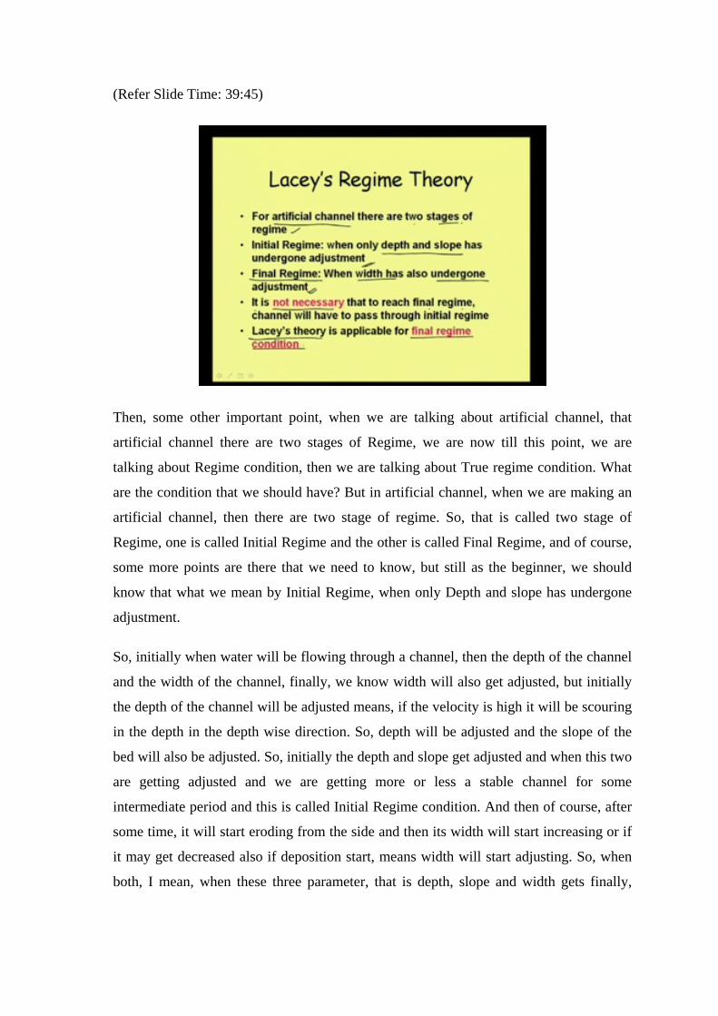
Then, some other important point, when we are talking about artificial channel, that

artificial channel there are two stages of Regime, we are now till this point, we are

talking about Regime condition, then we are talking about True regime condition. What

are the condition that we should have? But in artificial channel, when we are making an

artificial channel, then there are two stage of regime. So, that is called two stage of

Regime, one is called Initial Regime and the other is called Final Regime, and of course,

some more points are there that we need to know, but still as the beginner, we should

know that what we mean by Initial Regime, when only Depth and slope has undergone

adjustment.

So, initially when water will be flowing through a channel, then the depth of the channel

and the width of the channel, finally, we know width will also get adjusted, but initially

the depth of the channel will be adjusted means, if the velocity is high it will be scouring

in the depth in the depth wise direction. So, depth will be adjusted and the slope of the

bed will also be adjusted. So, initially the depth and slope get adjusted and when this two

are getting adjusted and we are getting more or less a stable channel for some

intermediate period and this is called Initial Regime condition. And then of course, after

some time, it will start eroding from the side and then its width will start increasing or if

it may get decreased also if deposition start, means width will start adjusting. So, when

both, I mean, when these three parameter, that is depth, slope and width gets finally,

adjusted, then this is called Final Regime condition. So, once we get Initial Regime, then

we call this as a Final Regime condition, when width has also undergone adjustment.

And in the entire process, the side slope is also getting adjusted. When we are talking

about Regime condition, we say that side slope will have its own value based on the

erosion and deposition. So, that way we are not providing a side slope directly here, that

we will assume that for the Regime Channel, this is the side slope. Of course, in

Kennedy’s theory, we were not talking about the side slope and based on the sediment

characteristics, we can have some side slope there, but here we are saying that in Lacey’s

Theory, side slope will get adjusted. In fact, he suggested some value for the side slope

or from observation, it can be taken that side slope can be taken as 0.5 is to 1, that is for

1 depth 0.5 width.

So, that way the side slope can be considered, but one more important point that I am

putting in red here is, you can concentrate in the slide, that it is not necessary that to

reach the Final Regime, the channel will have to pass through Initial regime. So, the

channel need not pass through Initial Regime to reach the Final Regime in all cases.

Normally of course, normally it goes first to Initial Regime, then it achieve its final

regime, but sometimes without passing through the Initial Regime, it can reach its Final

Regime. For example, suppose Final Regime width of the channel should be 5 meter for

example, and we have made a 6 meter wide channel and then the flow is flowing through

that, so, what will happen, the depth wise it is adjusting and then width is also getting

deposited, I mean channel sediment, that is carried by the channel may be depositing on

the side, because width is larger and that way by depositing finally, it is coming to the

width of 5 meter, which should be in the Regime condition and that way we may get a

Regime Channel, without passing through the Initial adjustment of only bed and slope.

So, I mean, that way this is not the necessary criteria and then more importantly Lacey’s

Theory, what he studied and based on his study, what are the Formula he has given those

are applicable for Final Regime condition. So, once we are designing a channel, we

should know that this channel, we are basically designing, considering that, this is the

Final Regime size and so, those Formula will be giving us this value.

(Refer Slide Time: 44:47)

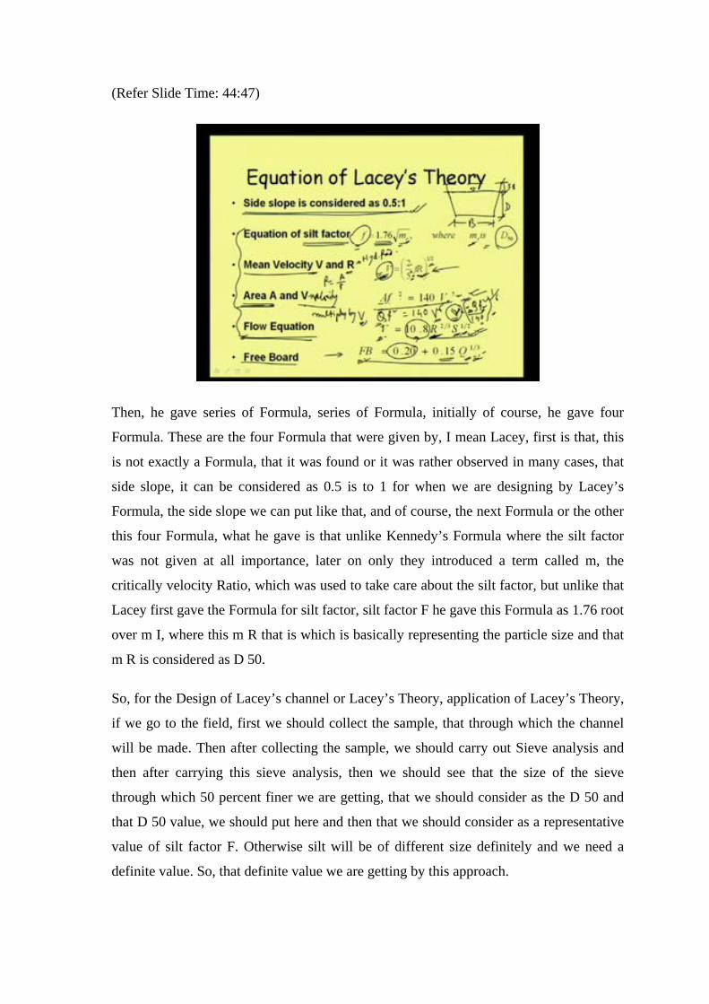
Then, he gave series of Formula, series of Formula, initially of course, he gave four

Formula. These are the four Formula that were given by, I mean Lacey, first is that, this

is not exactly a Formula, that it was found or it was rather observed in many cases, that

side slope, it can be considered as 0.5 is to 1 for when we are designing by Lacey’s

Formula, the side slope we can put like that, and of course, the next Formula or the other

this four Formula, what he gave is that unlike Kennedy’s Formula where the silt factor

was not given at all importance, later on only they introduced a term called m, the

critically velocity Ratio, which was used to take care about the silt factor, but unlike that

Lacey first gave the Formula for silt factor, silt factor F he gave this Formula as 1.76 root

over m I, where this m R that is which is basically representing the particle size and that

m R is considered as D 50.

So, for the Design of Lacey’s channel or Lacey’s Theory, application of Lacey’s Theory,

if we go to the field, first we should collect the sample, that through which the channel

will be made. Then after collecting the sample, we should carry out Sieve analysis and

then after carrying this sieve analysis, then we should see that the size of the sieve

through which 50 percent finer we are getting, that we should consider as the D 50 and

that D 50 value, we should put here and then that we should consider as a representative

value of silt factor F. Otherwise silt will be of different size definitely and we need a

definite value. So, that definite value we are getting by this approach.

Then, we should calculate the Mean Velocity and then he gave some relationship

between, in fact, he gave four relationship, one relationship is between the Mean

Velocity V and this R, R is nothing but hydraulic radius and that is what this a by P R is

equal to a by P. We know that in Manning’s Formula or in our Uniform Flow Formula

also, we relate this velocity to the hydraulic radius R and then we take care of the slope,

but here this is the velocity, which we try to achieve and then this velocity is equal to is

given as 2 by 5 rather root over 2 by 5 F R. Again silt factor is playing a role here. And

in fact, in all those formula, in most of the Formula that he has given the silt factor has a

vital role. So, the determination of the silt factor is very important. And then the V, we

can have 2 by 5 F into R to the power half. So, that relation he gave, then he gave

another relation. So, here also one relation for V and another relation he gave between

the area, that is the cross sectional area of flow and the velocity V.

So, between these velocity V and cross sectional area A again gave this relationship, that

a and F square, again the silt factor is coming here is equal to 140 into V to the power 5.

Now, this you can see very well, just I will show later this is one relationship. Then

another relationship he gave that is the Flow Equation. Normally, in Kennedy’s Formula

or in our Design of Uniform Flow channel also, we were using the Uniform Flow

Equation, that is V is equal to say 1 by n R to the power 2 by 3 and S to the power half

basis on Manning’s Formula. And there, we took that n value that can take different

value based on the material and when we are going into the field and we are seeing the

material, then what will be the n value taking a decision about, that is very difficult of

course, unless, we have a lot of experience on having seeing different type of material

and then experiencing how the depth of flow will be or whether the depth of flow, the

Uniform Flow Depth, we can have by using a particular numerical value for this n, but

here in Lacey’s Formula rather than giving 1 by n the other part is remaining same R to

the power 2 by 3, S to the power half, this part is remaining same as Manning’s formula.

But, he gave a value 10.8 by experimenting, by collecting data from different sources

from several portion he collected data, several stable section he observed and collected

data and he gave this formula, that velocity can be computed by using this direct

formula, where we need not be worried for the n value, rather we can take a definite

value of 10.8. So, that way when we try to compute, this computation become easy, but

of course, the limitations those are there, as we are considering a definite value, that is

having definitely some limitation and of course, this formula was not given directly and,

but still for freeboard in Lacey’s Formula, we can use this relation, it is actually not for

the channel design, but what he gave, that if the channel need to carry higher discharge,

freeboard means, if we have a channel like this, then say by design we are getting that

this much is the depth D and this is the bed width b.

So, we have got this design, but the channel, when we are putting in field, we cannot put

exactly equal to D, because due to many reason this depth can increase beyond that or

may be the wave are coming through this channel and that way also it can exceed this

limit. So, always it is necessary to provide a freeboard, suppose channel we are

constructing up to this much, our water depth is here, but we are always providing a

freeboard and he suggested that this freeboard should be more when discharge is more

and that way he gave a relationship, that is 0.2 plus 0.5 Q to the power 1 by 3. So, that

relationship was given by him. And now, just we want to discuss about this formula.

Another aspect, that is a F square is equal to, suppose 140 V to the power 5. This formula

if we multiply by V, then what will be getting, suppose if we multiply by V, then it will

become area into velocity.

And from the continuity condition, we know that continuity relation, we know that area

into velocity is nothing, but Q. And for Design of channel always. Well, in all this

formula, we are not talking about Q accept the free board, but in all these formula, we

are not about q, but channel we need to design for a given discharge, for a given

discharge and as such we should be careful about or we should be concerned about what

the Q value use. So, you can concentrate on the slide, that if we write here Q, just

multiplying by V, this formula will become Q F square and this is equal to 140 and V to

the power 6. Now, from this relation, just by multiplying V we can have another

equation, which is relating Q and V.

So, now we can write as V is equal to say Q F square by 140 to the power 1 by 6. So,

that way we can write, V is equal to Q F square by 140 into 1 by 6. So, this way; that

means, from 1 formula, suppose we want to say Q is given, then in practical field as I

have already explained, that taking the silt data we can find the F. Our target is to design

the channel for a particular discharge. So, rather Q is our required things it is given, F we

have obtained, then we can find what should be the velocity, then this V we can find out,

Q F square by 140 to the power 1 6. So, this equation can be manipulated to have

different relationship.

And, then we can try to see, if this V is to be achieved and say V is equal to from this

formula we can see what will be the relation between a and b sorry between V and y,

because R is a function of B and y, from here we are getting some value. And then here

we are or we can go by other way also. So, here it is R and if you put R here again slope

term is here and what will be the slope we should take or once we get the V value, then

we can go back to this formula, first formula, this one. In this Formula as we have got the

V, we put the V here by putting the V here, we can get what the value of R is because F

is already known. Getting that R, we can now put here R and we can get what slope

should be or that way we can indirectly calculate the advisable slope in that channel. In

fact, in some channel suppose of course, we say that natural terrain will govern the flow,

but we have a scope of adjusting the slope also in sometimes.

Suppose our terrain is having a particular slope, but if we increase, if we try to increase

the slope, we can align the slope in a curvilinear way like this and then we can have a

slope, different slope. So, like that we can adjust it to some extent. So, what I want to

emphasize from this point, that by manipulating these equation, we can have some

derived equation which were perhaps were not given by Lacey’s, but we can derive some

relation from these equation itself.

(Refer Slide Time: 56:33)

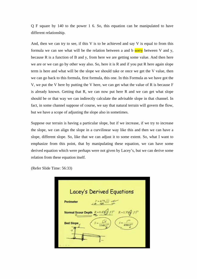
And one of those equations are, I mean some of those equations are very important and

we can directly use, one is the Perimeter p. So, as I have already explained that, we can

have from here, we are getting Q and then perimeter is equal to say R is equal to area by

perimeter that we are getting and area we can calculate from this continuity equation also

knowing the V and putting those value, we can then indirectly calculate P also. So, P in

terms of Q we can calculate and that Formula is 4.75 root over Q.

So, if Q is given or Q is our required thing, from there we can calculate the perimeter and

this perimeter in many a time is used for considering, suppose in a breeze, we are

considering and with 1 to reduce the water way, because the breeze will be smaller than

the actual width of the river. We narrow down the breeze portion for economy purpose.

Then P will indicate what should be the minimum width of the breeze. Otherwise our

perimeter will further reduce and then it will not be in Regime condition in nature. So, to

have the channel in Regime condition or to not to violate the Regime condition in a

much way, this P is used for that purpose also, finding the minimum water way in breeze

and different purpose also we use.

Similarly, the scour depth, this is also used for design of many hydraulic structure, that

what will be the R. That R means, we are calculating by indirectly from these formula,

that is Q f and these are coming, this is in terms of total discharge, this is in terms of unit

discharge, and by using these things we are getting R, because this is in Regime

condition this will be. Suppose, in a channel we are having this much of depth, but we

know that it will get eroded and then it will be depositing, it may deposit or it may erode

if the depth is less, suppose it will be flowing in this depth, then suppose its Regime

condition depth is much higher, then it will be eroding and the ultimate depth may come

up to this portion and then if we are constructing a hydraulic structure here, then if this

water eroded up to this much depth this hydraulic structure will not remain, it will be

washed away.

So, we have to provide some provision. So, we are putting some barrier here. So, that

this erosion even if it comes to this much of depth, it will not take this hydraulic structure

away and this is called cut of sort of things, and for designing those things, we use this

scour Depth, that is why it is called scour Depth, because this is the depth in Regime

condition and of course, this is the Normal Scour depth, but in again, depending on some

other criteria, that is bend, if it is straight, then we need to for design purpose, we need to

take some safe curve. So, we get the actual scour Depth we can multiply it by some

factor and similarly Bed Slope we can calculate using this friction factor, I mean silt

factor and this discharge and of course, by two different way, if we calculate we get two

different formula and these two different formula will of course, not give identical value,

one is relating R, one is relating Q, but both the way we can go and it will gives us some

tentative value for this Q for this bed slope.

So, all these formula, we can apply for Design of channel by using Lacey’s Formula.

And as discussed, there are some limitation and practical knowledge of the practical field

of a particular region is very important to apply this equation in more confident way.

Then some other methods are there as we explain, attractive force method and those will

be discussing in our next class.