program for the stereochemical analysis of molecular
TRANSCRIPT
SHAPE
Program for the Stereochemical Analysis of Molecular Fragments by Means of
Continuous Shape Measures and Associated Tools
User's Manual Version 2.1, March 2013
Miquel Llunell,† David Casanova, Jordi Cirera, Pere Alemany and Santiago Alvarez
Departament de Química Física, Departament de Química Inorgànica, and Institut de
Química Teòrica i Computacional - Universitat de Barcelona
† e-mail: [email protected]
Shape 2.1 – User's Manual [2]
TABLE OF CONTENTS
About Shape 3
Using Shape 3
Standard input file 3
Reference polyhedra 4
Input using an external atomic coordinates file 5
Output files 6
Minimal distortion paths 6
Selecting structures with stereochemical criteria 6
User-defined reference shapes 7
Acknowledgments 7
List of reference shapes 8
File extensions 11
Optional keywords 12
Examples and sample files 14
Shape 2.1 – User's Manual [3]
About Shape
Shape calculates continuous shape measures (CShM's) of a set of points (e.g. atomic positions) relative to the vertices of ideal reference polygons or polyhedra (referred in general as "polyhedra" from here on for simplicity), either centered or non centered. The non centered polyhedra are intended to represent structures of clusters without a central atom, whereas centered polyhedra typically represent the coordination sphere (vertices) of a central atom. Throughout this manual we will indistinctly refer to vertices and atoms as synonims. Shape also calculates deviations from minimal distortion paths and polyhedral interconversion generalized coordinates. This program is based on the algorithm described by Pinsky and Avnir for the calculation of continuous shape measures, and on the definitions of minimal distortion paths and generalized interconversion coordinates. For more information see the following references:
- Continuous shape measures algorithm: M. Pinsky, D. Avnir. Inorg. Chem., 37, 5575 (1998). - Minimal distortion paths: D. Casanova, J. Cirera, M. Llunell, P. Alemany, D. Avnir,
S. Alvarez. J. Am. Chem. Soc., 126, 1755-1763 (2004). - Generalized interconversion coordinates: J. Cirera, E. Ruiz, S. Alvarez.
Chem. Eur. J., 12, 3162 (2006).
It must be noticed that the algorithm used by Shape does not distinguish the two enantiomers of a chiral shape. Therefore, whenever a chiral reference polyhedron is used, the resulting shape measures may not refer to that specific polyhedron but to its enantiomer.
Using Shape
To run the program for calculating shape measures you must simply type shape name[.dat]
assuming the executable has the name "shape" and the input data is in a file name.dat (the file name can be given with or without extension). The program will write the results in the name.tab file and additional output files as required by optional keywords.
Alternatively, you may inquire the codes that identify the n-vertex reference polyhedra by typing
shape +[n]
If the number of vertices is not given, Shape gives a list of all available reference polyhedra. To obtain a list of optional keywords type
shape -h
Standard Input File (See Example 1 for a sample input file)
The input file must have the extension .dat (e.g.: name.dat), and a name not exceeding 40 characters. It may contain at any position blank lines or comment lines starting by "!". The
Shape 2.1 – User's Manual [4]
program reads all other lines in free format, allowing for any number of blank spaces between the data, and any number of digits for numerical data.
The input file may contain the following data (fields 1-3 are optional, while field 6 can be omitted if a keyword for reading an external coordinates file is used).
1• Title line (up to 80 characters) indicated by the ‘$’ symbol in the first column.
2• Optional comment lines, recognized by the "!" symbol in the first column, allowed at any position of the input file.
3• Keywords (one line for each keyword)
4• Size of the polyhedron (two integer parameters): - Number of vertices - Position of the central atom in the coordinates list (0 if there is no central atom); it must be the same for all the structures.
5• Codes of the reference polyhedra chosen (up to 12). These codes can be found in a table below, or can be obtained on screen by typing the symbol "+" when prompted for the input file name (all polyhedra), or "+n" (only polyhedra with n vertices).
6• One data set for each structure to be analyzed that comprises: • A label for the structure with up to 15 characters (e.g., the refcode of a CSD structure). • One line per atom containing a label with up to 4 characters (e.g., an atomic symbol) and cartesian coordinates.
Reference Polyhedra
The ideal geometries of some 90 reference polyhedra are internally defined in Shape , and identified by acronyms analogous to those defined by IUPAC for some of them. Those geometries meet the following criteria: (i) Regular and semiregular reference polyhedra have all edges of the same length and are spherical (i.e., their vertices are equidistant to the geometric center); this includes the Platonic solids, the prisms and the antiprisms, but not the bipyramids. (ii) For some polyhedra two or more alternative reference shapes are provided, e.g., a spherical version with all center-to-vertex distances identical (best suited for coordination polyhedra), a Johnson version with all edges identical (best suited for clusters or boranes), whose acronym starts with a capital J, and a polyhedron with vacant positions (whose acronyms start with a lower case v). More information about reference shapes other than regular polyhedra can be found in our publications:
- Four vertex polyhedra: J. Cirera, P. Alemany, S. Alvarez. Chem. Eur. J. 10, 190 (2004). - Five vertex polyhedra: S. Alvarez, M. Llunell. J. Chem. Soc., Dalton Trans. 3288 (2000). - Six vertex polyhedra: S. Alvarez, D. Avnir, M. Llunell, M. Pinsky. New J. Chem. 26, 996
(2002). - Seven vertex polyhedra: D. Casanova, P. Alemany, J. M. Bofill, S. Alvarez. Chem. Eur. J. 9,
1281 (2003). - Eight vertex polyhedra: D. Casanova, M. Llunell, P. Alemany, S. Alvarez. Chem. Eur. J. 11,
1479 (2005).
Shape 2.1 – User's Manual [5]
- Nine vertex polyhedra: A. Ruiz-Martínez, D. Casanova, S. Alvarez. Chem. Eur. J. 14, 1291 (2008); Dalton Trans., 2583 (2008)
- Ten vertex polyhedra: A. Ruiz-Martínez, D. Casanova, S. Alvarez. Chem. Eur. J. 15, 7470 (2009).
- Twelve, Twenty and Sixty vertex polyhedra: J. Echeverría, D. Casanova, M. Llunell, P. Alemany, S. Alvarez, Chem. Commun. 2717 (2008); S. Alvarez, Inorg. Chim. Acta 363, 4392 (2010).
- Cubic Lattices: J. Echeverría, D. Casanova, M. Llunell, P. Alemany, S. Alvarez, Chem. Commun. 2717 (2008).
- Ill-defined coordination numbers and association-dissociation paths: A. Ruiz-Martínez, D. Casanova, S. Alvarez. Chem. Eur. J. 16, 6567 (2010).
- Reviews: S. Alvarez, P. Alemany, D. Casanova, J. Cirera, M. Llunell, D. Avnir. Coord. Chem. Rev. 249, 1693 (2005); S. Alvarez, E. Ruiz, in Supramolecular Chemistry, From Molecules to Nanomaterials, J. W. Steed, P. A. Gale, eds., John Wiley & Sons, Chichester, UK, Vol. 5, 1993-2044 (2012).
Input Using an External Atomic Coordinates File
Shape is able to handle a large number of structures using atomic coordinate files generated by other programs or downloaded from the Cambridge Structural Database. To use such coordinate files you only need to include before the first numerical data line a keyword that indicates the file type (%conquest or %external) and the name of the coordinates file to be used (optional). In such cases, no coordinates are required in the input file. The user must make sure that all the required data files are in the same directory from which the program is called.
%conquest
With this keyword, Shape fetches the coordinates from a file with the extension .cor, generated by the CSD ConQuest program. Be sure to check the "orthogonal coordinates" and "hit fragment only" options when exporting the coordinates from within ConQuest; the search fragment must have only the atoms corresponding to the vertices and center of the polyhedron. See Example 2.
– NEW – With this option, the output .tab file includes the refcode and the label of the central atom for each structure, allowing to distinguish crystallographicaly non equivalent fragments within the same crystal structure.
%external
With this keyword, Shape fetches the coordinates from a file with the extension .shp, with the same format as the item 6 in the .dat file, in which blank and comment lines are also allowed (see Example 3 for a sample file).
If the name of the .cor or .shp file is not specified, Shape searches a file with the same name as the data file. If the name of the coordinates file is specified, it can go with or without extension (i.e., both %conquest name and %conquest name.cor are valid).
Shape 2.1 – User's Manual [6]
Output Files
Shape writes in a file with the .tab extension and the same root as the input (.dat) file. Other output files are generated when special options are activated (see the "Optional Keywords" and "File Extensions" sections below).
Minimal Distortion Paths
The stereochemistry of structures intermediate between two reference shapes can be characterized by comparison to the minimal distortion path between those two shapes. Shape calculates the deviation from the minimal distortion path and the generalized coordinate along that path when the %path keyword is included. In that case only two reference shapes can be selected (see Example 5). Since generalized coordinates are meaningful only for those structures that fall along the minimal distortion path, the values given should be taken only as approximate for structures that significantly deviate from that path. For that reason, only generalized coordinates for structures that deviate less than a threshold value from the minimal distortion path are given in the output (.tab) file. The default threshold is set internally at 10%, but can be modified by the user with the help of the %maxdev keyword.
– NEW – With the %path option, version 2.1 generates a set of shape measures relative to the two ideal polyhedra chosen (.pth file), that can be used to represent the minimal distortion pathway in a shape map.
– NEW – The combined use of the %path and %test keywords generates an .xyz file with the coordinates of 21 ideal structures along the minimal distortion pathway, that can be used to make a movie of the interconversion of the two ideal polyhedra (see example 14). In that case, the .tab file is not generated.
Selecting Structures with Stereochemical Criteria
A set of structures can be filtered, discarding those that do not meet one of three stereochemical criteria, and the filtered results are written in the name.flt (text) and name.flt.csv (table) files. The applicable stereochemical criteria are: (i) CShM relative to a reference polyhedron below (or above) a chosen threshold (activated with the %maxcsm and %mincsm keywords, respectively), (ii) deviation from a minimal distortion pathway smaller or larger than a chosen value (%maxdev and %mindev keywords, respectively), and (iii) generalized coordinate along a minimal distortion pathway within a certain range (%mingco and %maxgco keywords). Shape generates the usual output file for all structures (.tab file), together with a file that contains only the filtered structures (.flt file). See Examples 6 and 7.
Shape 2.1 – User's Manual [7]
User-Defined Reference Shapes
Shape can also calculate measures relative to a user-defined reference shape. You only need to prepare a name.ref file with the coordinates of your reference shapes (as many as you wish) and use 0 in the input file as the code for each user-defined reference polyhedron (see Example 8). The contents of a .ref file are as follows:
- Abbreviation for the name of the ideal shape (up to 12 characters). - A line with a more detailed description of the reference shape (up to 50 characters). - Symmetry label (up to 5 characters) - Coordinates of the atoms occupying the vertices, followed by those of the central atom if present. Note that in the name.ref files the central atom (if present) must always be at the end of the list of coordinates, regardless of how are the coordinates of the problem structures arranged in the name.dat, name.cor or name.shp files.
Acknowledgments
The present expanded version of Shape would have not been possible without the collaboration
of David Avnir, Mark Pinsky and Josep M. Bofill in the development of the previous versions. The
authors and users of Shape are in debt with them.
Shape 2.1 – User's Manual [8]
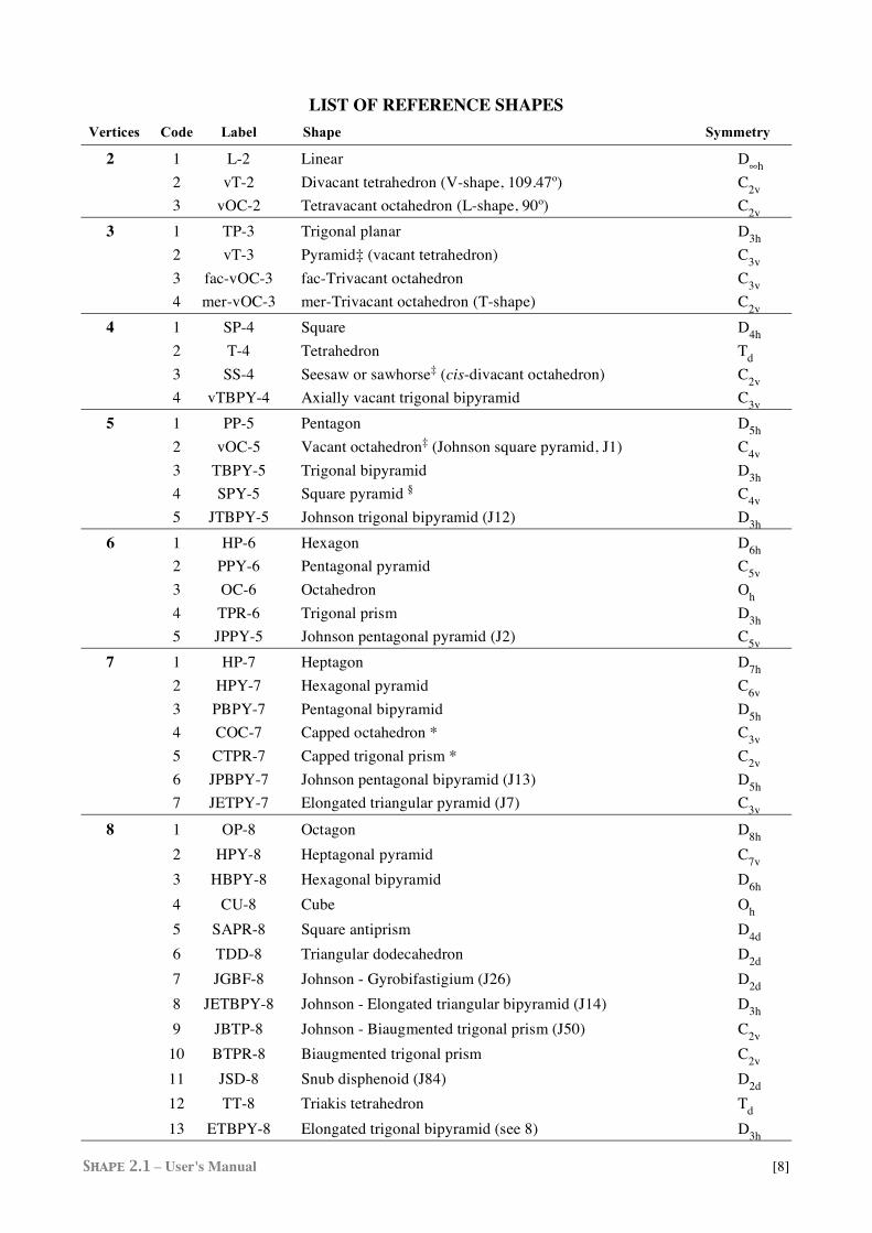
LIST OF REFERENCE SHAPES Vertices Code Label Shape Symmetry
2 1 L-2 Linear D∞h 2 vT-2 Divacant tetrahedron (V-shape, 109.47º) C2v 3 vOC-2 Tetravacant octahedron (L-shape, 90º) C2v 3 1 TP-3 Trigonal planar D3h 2 vT-3 Pyramid‡ (vacant tetrahedron) C3v 3 fac-vOC-3 fac-Trivacant octahedron C3v 4 mer-vOC-3 mer-Trivacant octahedron (T-shape) C2v 4 1 SP-4 Square D4h 2 T-4 Tetrahedron Td 3 SS-4 Seesaw or sawhorse‡ (cis-divacant octahedron) C2v 4 vTBPY-4 Axially vacant trigonal bipyramid C3v 5 1 PP-5 Pentagon D5h 2 vOC-5 Vacant octahedron‡ (Johnson square pyramid, J1) C4v 3 TBPY-5 Trigonal bipyramid D3h 4 SPY-5 Square pyramid § C4v 5 JTBPY-5 Johnson trigonal bipyramid (J12) D3h 6 1 HP-6 Hexagon D6h 2 PPY-6 Pentagonal pyramid C5v 3 OC-6 Octahedron Oh 4 TPR-6 Trigonal prism D3h 5 JPPY-5 Johnson pentagonal pyramid (J2) C5v 7 1 HP-7 Heptagon D7h 2 HPY-7 Hexagonal pyramid C6v 3 PBPY-7 Pentagonal bipyramid D5h 4 COC-7 Capped octahedron * C3v 5 CTPR-7 Capped trigonal prism * C2v 6 JPBPY-7 Johnson pentagonal bipyramid (J13) D5h 7 JETPY-7 Elongated triangular pyramid (J7) C3v 8 1 OP-8 Octagon D8h 2 HPY-8 Heptagonal pyramid C7v 3 HBPY-8 Hexagonal bipyramid D6h 4 CU-8 Cube Oh 5 SAPR-8 Square antiprism D4d 6 TDD-8 Triangular dodecahedron D2d 7 JGBF-8 Johnson - Gyrobifastigium (J26) D2d 8 JETBPY-8 Johnson - Elongated triangular bipyramid (J14) D3h 9 JBTP-8 Johnson - Biaugmented trigonal prism (J50) C2v 10 BTPR-8 Biaugmented trigonal prism C2v 11 JSD-8 Snub disphenoid (J84) D2d 12 TT-8 Triakis tetrahedron Td 13 ETBPY-8 Elongated trigonal bipyramid (see 8) D3h
Shape 2.1 – User's Manual [9]
Vertices Code Label Shape Symmetry
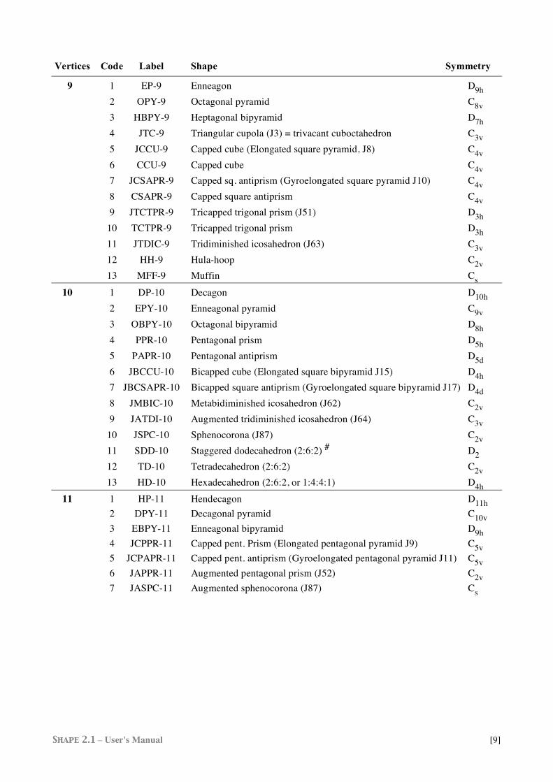
9 1 EP-9 Enneagon D9h 2 OPY-9 Octagonal pyramid C8v 3 HBPY-9 Heptagonal bipyramid D7h 4 JTC-9 Triangular cupola (J3) = trivacant cuboctahedron C3v 5 JCCU-9 Capped cube (Elongated square pyramid, J8) C4v 6 CCU-9 Capped cube C4v 7 JCSAPR-9 Capped sq. antiprism (Gyroelongated square pyramid J10) C4v 8 CSAPR-9 Capped square antiprism C4v 9 JTCTPR-9 Tricapped trigonal prism (J51) D3h 10 TCTPR-9 Tricapped trigonal prism D3h 11 JTDIC-9 Tridiminished icosahedron (J63) C3v 12 HH-9 Hula-hoop C2v 13 MFF-9 Muffin Cs 10 1 DP-10 Decagon D10h 2 EPY-10 Enneagonal pyramid C9v 3 OBPY-10 Octagonal bipyramid D8h 4 PPR-10 Pentagonal prism D5h 5 PAPR-10 Pentagonal antiprism D5d 6 JBCCU-10 Bicapped cube (Elongated square bipyramid J15) D4h 7 JBCSAPR-10 Bicapped square antiprism (Gyroelongated square bipyramid J17) D4d 8 JMBIC-10 Metabidiminished icosahedron (J62) C2v 9 JATDI-10 Augmented tridiminished icosahedron (J64) C3v 10 JSPC-10 Sphenocorona (J87) C2v 11 SDD-10 Staggered dodecahedron (2:6:2) # D2 12 TD-10 Tetradecahedron (2:6:2) C2v 13 HD-10 Hexadecahedron (2:6:2, or 1:4:4:1) D4h 11 1 HP-11 Hendecagon D11h 2 DPY-11 Decagonal pyramid C10v 3 EBPY-11 Enneagonal bipyramid D9h 4 JCPPR-11 Capped pent. Prism (Elongated pentagonal pyramid J9) C5v 5 JCPAPR-11 Capped pent. antiprism (Gyroelongated pentagonal pyramid J11) C5v 6 JAPPR-11 Augmented pentagonal prism (J52) C2v 7 JASPC-11 Augmented sphenocorona (J87) Cs
Shape 2.1 – User's Manual [10]
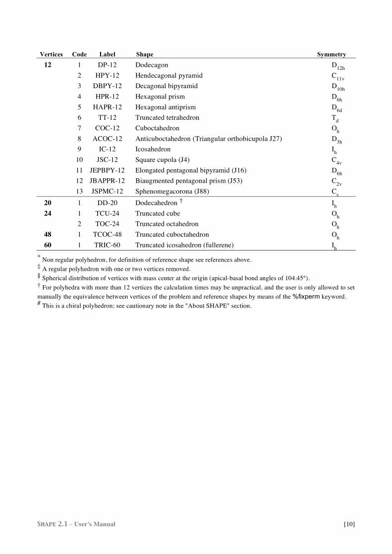
Vertices Code Label Shape Symmetry 12 1 DP-12 Dodecagon D12h 2 HPY-12 Hendecagonal pyramid C11v 3 DBPY-12 Decagonal bipyramid D10h 4 HPR-12 Hexagonal prism D6h 5 HAPR-12 Hexagonal antiprism D6d 6 TT-12 Truncated tetrahedron Td 7 COC-12 Cuboctahedron Oh 8 ACOC-12 Anticuboctahedron (Triangular orthobicupola J27) D3h 9 IC-12 Icosahedron Ih 10 JSC-12 Square cupola (J4) C4v 11 JEPBPY-12 Elongated pentagonal bipyramid (J16) D6h 12 JBAPPR-12 Biaugmented pentagonal prism (J53) C2v 13 JSPMC-12 Sphenomegacorona (J88) Cs 20 1 DD-20 Dodecahedron † Ih 24 1 TCU-24 Truncated cube Oh 2 TOC-24 Truncated octahedron Oh 48 1 TCOC-48 Truncated cuboctahedron Oh 60 1 TRIC-60 Truncated icosahedron (fullerene) Ih * Non regular polyhedron, for definition of reference shape see references above. ‡ A regular polyhedron with one or two vertices removed. § Spherical distribution of vertices with mass center at the origin (apical-basal bond angles of 104.45°). † For polyhedra with more than 12 vertices the calculation times may be unpractical, and the user is only allowed to set manually the equivalence between vertices of the problem and reference shapes by means of the %fixperm keyword. # This is a chiral polyhedron; see cautionary note in the "About SHAPE" section.
Shape 2.1 – User's Manual [11]
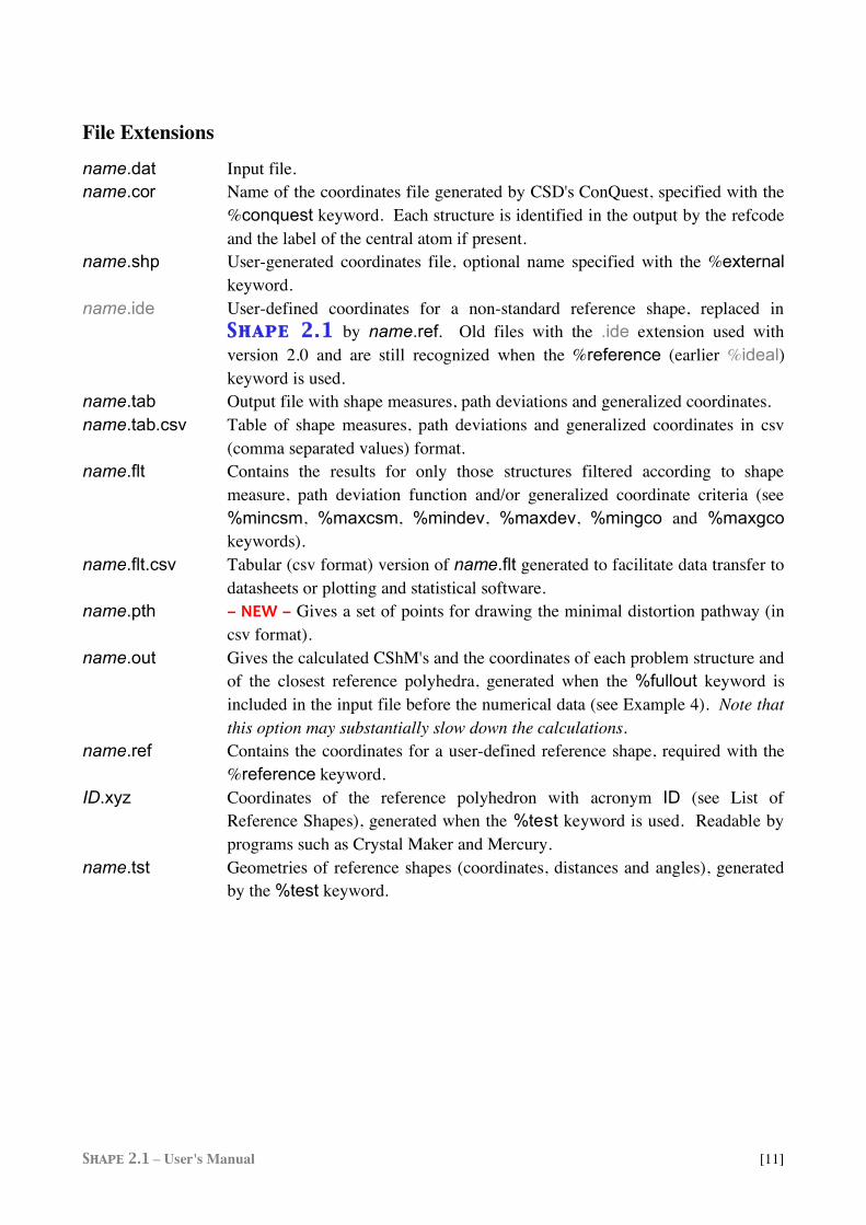
File Extensions
name.dat Input file. name.cor Name of the coordinates file generated by CSD's ConQuest, specified with the
%conquest keyword. Each structure is identified in the output by the refcode and the label of the central atom if present.
name.shp User-generated coordinates file, optional name specified with the %external keyword.
name.ide User-defined coordinates for a non-standard reference shape, replaced in Shape 2.1 by name.ref. Old files with the .ide extension used with version 2.0 and are still recognized when the %reference (earlier %ideal) keyword is used.
name.tab Output file with shape measures, path deviations and generalized coordinates. name.tab.csv Table of shape measures, path deviations and generalized coordinates in csv
(comma separated values) format. name.flt Contains the results for only those structures filtered according to shape
measure, path deviation function and/or generalized coordinate criteria (see %mincsm, %maxcsm, %mindev, %maxdev, %mingco and %maxgco keywords).
name.flt.csv Tabular (csv format) version of name.flt generated to facilitate data transfer to datasheets or plotting and statistical software.
name.pth – NEW – Gives a set of points for drawing the minimal distortion pathway (in csv format).
name.out Gives the calculated CShM's and the coordinates of each problem structure and of the closest reference polyhedra, generated when the %fullout keyword is included in the input file before the numerical data (see Example 4). Note that this option may substantially slow down the calculations.
name.ref Contains the coordinates for a user-defined reference shape, required with the %reference keyword.
ID.xyz Coordinates of the reference polyhedron with acronym ID (see List of Reference Shapes), generated when the %test keyword is used. Readable by programs such as Crystal Maker and Mercury.
name.tst Geometries of reference shapes (coordinates, distances and angles), generated by the %test keyword.
Shape 2.1 – User's Manual [12]
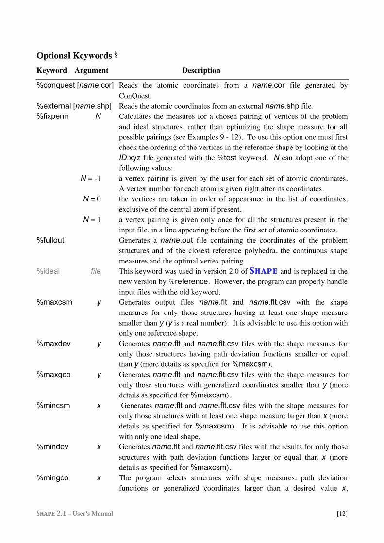
Optional Keywords § Keyword Argument Description
%conquest [name.cor] Reads the atomic coordinates from a name.cor file generated by ConQuest.
%external [name.shp] Reads the atomic coordinates from an external name.shp file. %fixperm N Calculates the measures for a chosen pairing of vertices of the problem
and ideal structures, rather than optimizing the shape measure for all possible pairings (see Examples 9 - 12). To use this option one must first check the ordering of the vertices in the reference shape by looking at the ID.xyz file generated with the %test keyword. N can adopt one of the following values:
N = -1 a vertex pairing is given by the user for each set of atomic coordinates. A vertex number for each atom is given right after its coordinates.
N = 0 the vertices are taken in order of appearance in the list of coordinates, exclusive of the central atom if present.
N = 1 a vertex pairing is given only once for all the structures present in the input file, in a line appearing before the first set of atomic coordinates.
%fullout Generates a name.out file containing the coordinates of the problem structures and of the closest reference polyhedra, the continuous shape measures and the optimal vertex pairing.
%ideal file This keyword was used in version 2.0 of Shape and is replaced in the new version by %reference. However, the program can properly handle input files with the old keyword.
%maxcsm y Generates output files name.flt and name.flt.csv with the shape measures for only those structures having at least one shape measure smaller than y (y is a real number). It is advisable to use this option with only one reference shape.
%maxdev y Generates name.flt and name.flt.csv files with the shape measures for only those structures having path deviation functions smaller or equal than y (more details as specified for %maxcsm).
%maxgco y Generates name.flt and name.flt.csv files with the shape measures for only those structures with generalized coordinates smaller than y (more details as specified for %maxcsm).
%mincsm x Generates name.flt and name.flt.csv files with the shape measures for only those structures with at least one shape measure larger than x (more details as specified for %maxcsm). It is advisable to use this option with only one ideal shape.
%mindev x Generates name.flt and name.flt.csv files with the results for only those structures with path deviation functions larger or equal than x (more details as specified for %maxcsm).
%mingco x The program selects structures with shape measures, path deviation functions or generalized coordinates larger than a desired value x,
Shape 2.1 – User's Manual [13]
respectively, and writes the filtered results to the name.flt and name.flt.csv files.
NOTE: The combined use of %maxxxx and %minxxx keywords allows one to select structures within a specific range (between x and y) of, e.g., generalized coordinates (see Examples 6 and 7). With those options, name.flt and name.flt.csv files are generated, containing the full output for the filtered structures and a table with only the numerical values in the csv (comma separated values) format, respectively.
%nosymbol Indicates that no atomic labels are included with the coordinates. %path Calculates the path deviation function for the minimal distortion
interconversion path between two given polyhedra as well as the generalized coordinate. Two and only two reference polyhedra should be coded in the input file with this option. The path is assumed to go from the first (0%) to the second (100%) reference shape specified in the input file.
The generalized coordinate is given only for structures that deviate at most a 10% from the minimal distortion interconversion path. This threshold can be modified with the %maxdev keyword.
%reference file Points to a file.ref file containing user-defined reference shapes. The name of the file must be specified only if it is different from that of the data file (see Example 8). This keyword replaces the %ideal keyword of version 2.0 of Shape , but the program can properly handle input files with the old keyword.
%select label Performs shape measures only for the set of coordinates under the structure label specified and places the results in a file with the name label.
%stop N Calculates the shape measures for the first N structures only. %test Generates a .tst file with the geometries of the reference shapes
(coordinates, distances and angles), and one .xyz file for each ideal shape. The input file must specify the number of vertices and the code of the reference shapes, but no atomic coordinates are required (see Example 13).
%thrdev x This option is replaced in Shape 2.1 by the %mindev and %maxdev keywords.
§ Keywords must appear in the input file before the numerical data.
Shape 2.1 – User's Manual [14]
Shape
Examples and Sample Files
Example 1: Standard input file 15
Example 2: Atomic coordinates from a .cor file generated by CSD's ConQuest 16
Example 3: Input with external coordinates 17
Example 4: Use of the %fullout keyword 17
Example 5: Deviation from minimal distortion pathways 19
Example 6: Use of the %maxdev keyword 21
Example 7: Use of the %maxgco and %mingco keywords 23
Example 8: Use of a user-defined reference polyhedron 24
Example 9. Large polyhedra: specifying a vertex pairing with the %fixperm option 25
Example 10: Truncated Icosahedron 29
Examples 11 and 12: Other %fixperm options 31
Example 13: Getting coordinates of internally defined ideal shapes 34
Example 14: Generating coordinates of structures along a minimal distortion path 34
Shape 2.1 – User's Manual [15]
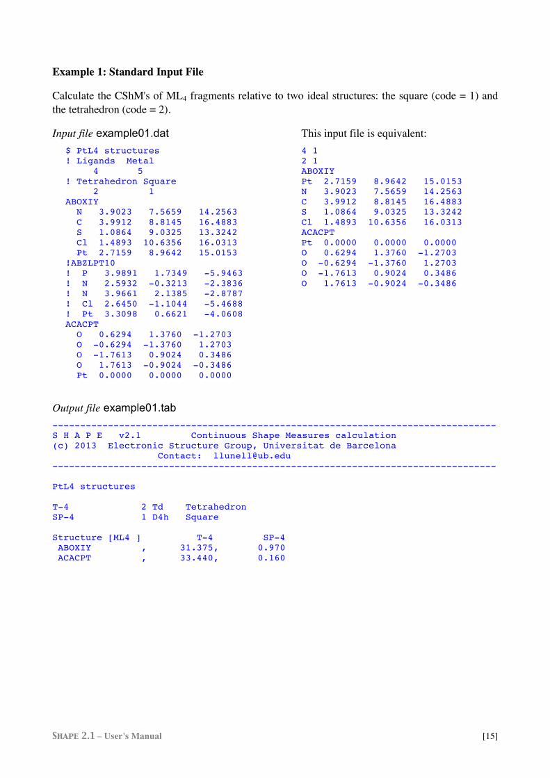
Example 1: Standard Input File
Calculate the CShM's of ML4 fragments relative to two ideal structures: the square (code = 1) and the tetrahedron (code = 2).
Input file example01.dat This input file is equivalent: $ PtL4 structures 4 1 ! Ligands Metal 2 1 4 5 ABOXIY ! Tetrahedron Square Pt 2.7159 8.9642 15.0153 2 1 N 3.9023 7.5659 14.2563 ABOXIY C 3.9912 8.8145 16.4883 N 3.9023 7.5659 14.2563 S 1.0864 9.0325 13.3242 C 3.9912 8.8145 16.4883 Cl 1.4893 10.6356 16.0313 S 1.0864 9.0325 13.3242 ACACPT Cl 1.4893 10.6356 16.0313 Pt 0.0000 0.0000 0.0000 Pt 2.7159 8.9642 15.0153 O 0.6294 1.3760 -1.2703 !ABZLPT10 O -0.6294 -1.3760 1.2703 ! P 3.9891 1.7349 -5.9463 O -1.7613 0.9024 0.3486 ! N 2.5932 -0.3213 -2.3836 O 1.7613 -0.9024 -0.3486 ! N 3.9661 2.1385 -2.8787 ! Cl 2.6450 -1.1044 -5.4688 ! Pt 3.3098 0.6621 -4.0608 ACACPT O 0.6294 1.3760 -1.2703 O -0.6294 -1.3760 1.2703 O -1.7613 0.9024 0.3486 O 1.7613 -0.9024 -0.3486 Pt 0.0000 0.0000 0.0000
Output file example01.tab -------------------------------------------------------------------------------- S H A P E v2.1 Continuous Shape Measures calculation (c) 2013 Electronic Structure Group, Universitat de Barcelona Contact: [email protected] -------------------------------------------------------------------------------- PtL4 structures T-4 2 Td Tetrahedron SP-4 1 D4h Square Structure [ML4 ] T-4 SP-4 ABOXIY , 31.375, 0.970 ACACPT , 33.440, 0.160
Shape 2.1 – User's Manual [16]
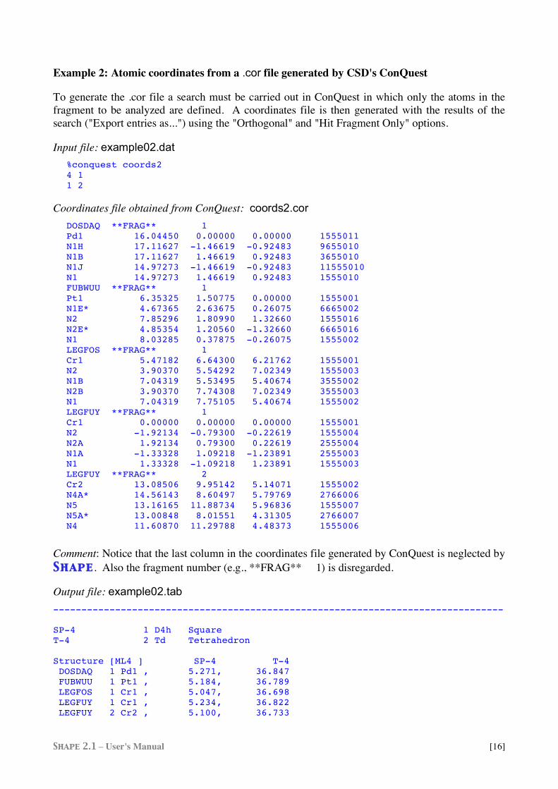
Example 2: Atomic coordinates from a .cor file generated by CSD's ConQuest
To generate the .cor file a search must be carried out in ConQuest in which only the atoms in the fragment to be analyzed are defined. A coordinates file is then generated with the results of the search ("Export entries as...") using the "Orthogonal" and "Hit Fragment Only" options.
Input file: example02.dat %conquest coords2 4 1 1 2
Coordinates file obtained from ConQuest: coords2.cor DOSDAQ **FRAG** 1 Pd1 16.04450 0.00000 0.00000 1555011 N1H 17.11627 -1.46619 -0.92483 9655010 N1B 17.11627 1.46619 0.92483 3655010 N1J 14.97273 -1.46619 -0.92483 11555010 N1 14.97273 1.46619 0.92483 1555010 FUBWUU **FRAG** 1 Pt1 6.35325 1.50775 0.00000 1555001 N1E* 4.67365 2.63675 0.26075 6665002 N2 7.85296 1.80990 1.32660 1555016 N2E* 4.85354 1.20560 -1.32660 6665016 N1 8.03285 0.37875 -0.26075 1555002 LEGFOS **FRAG** 1 Cr1 5.47182 6.64300 6.21762 1555001 N2 3.90370 5.54292 7.02349 1555003 N1B 7.04319 5.53495 5.40674 3555002 N2B 3.90370 7.74308 7.02349 3555003 N1 7.04319 7.75105 5.40674 1555002 LEGFUY **FRAG** 1 Cr1 0.00000 0.00000 0.00000 1555001 N2 -1.92134 -0.79300 -0.22619 1555004 N2A 1.92134 0.79300 0.22619 2555004 N1A -1.33328 1.09218 -1.23891 2555003 N1 1.33328 -1.09218 1.23891 1555003 LEGFUY **FRAG** 2 Cr2 13.08506 9.95142 5.14071 1555002 N4A* 14.56143 8.60497 5.79769 2766006 N5 13.16165 11.88734 5.96836 1555007 N5A* 13.00848 8.01551 4.31305 2766007 N4 11.60870 11.29788 4.48373 1555006
Comment: Notice that the last column in the coordinates file generated by ConQuest is neglected by Shape . Also the fragment number (e.g., **FRAG** 1) is disregarded.
Output file: example02.tab -------------------------------------------------------------------------------- SP-4 1 D4h Square T-4 2 Td Tetrahedron Structure [ML4 ] SP-4 T-4 DOSDAQ 1 Pd1 , 5.271, 36.847 FUBWUU 1 Pt1 , 5.184, 36.789 LEGFOS 1 Cr1 , 5.047, 36.698 LEGFUY 1 Cr1 , 5.234, 36.822 LEGFUY 2 Cr2 , 5.100, 36.733
Shape 2.1 – User's Manual [17]
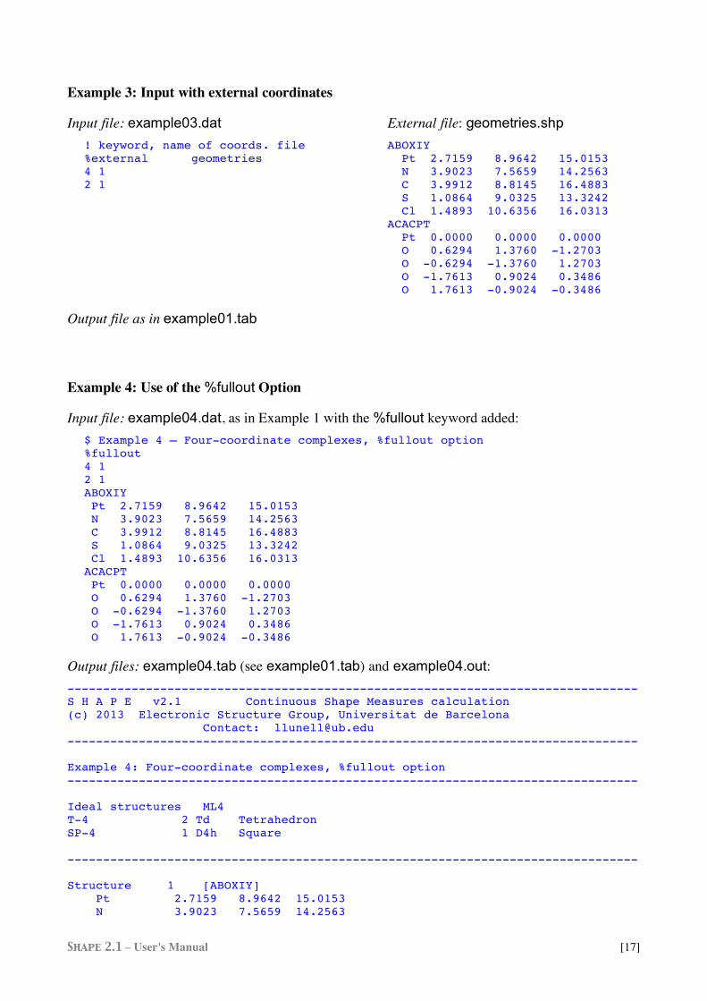
Example 3: Input with external coordinates
Input file: example03.dat External file: geometries.shp ! keyword, name of coords. file ABOXIY %external geometries Pt 2.7159 8.9642 15.0153 4 1 N 3.9023 7.5659 14.2563 2 1 C 3.9912 8.8145 16.4883 S 1.0864 9.0325 13.3242 Cl 1.4893 10.6356 16.0313 ACACPT Pt 0.0000 0.0000 0.0000 O 0.6294 1.3760 -1.2703 O -0.6294 -1.3760 1.2703 O -1.7613 0.9024 0.3486 O 1.7613 -0.9024 -0.3486
Output file as in example01.tab
Example 4: Use of the %fullout Option
Input file: example04.dat, as in Example 1 with the %fullout keyword added: $ Example 4 – Four-coordinate complexes, %fullout option %fullout 4 1 2 1 ABOXIY Pt 2.7159 8.9642 15.0153 N 3.9023 7.5659 14.2563 C 3.9912 8.8145 16.4883 S 1.0864 9.0325 13.3242 Cl 1.4893 10.6356 16.0313 ACACPT Pt 0.0000 0.0000 0.0000 O 0.6294 1.3760 -1.2703 O -0.6294 -1.3760 1.2703 O -1.7613 0.9024 0.3486 O 1.7613 -0.9024 -0.3486
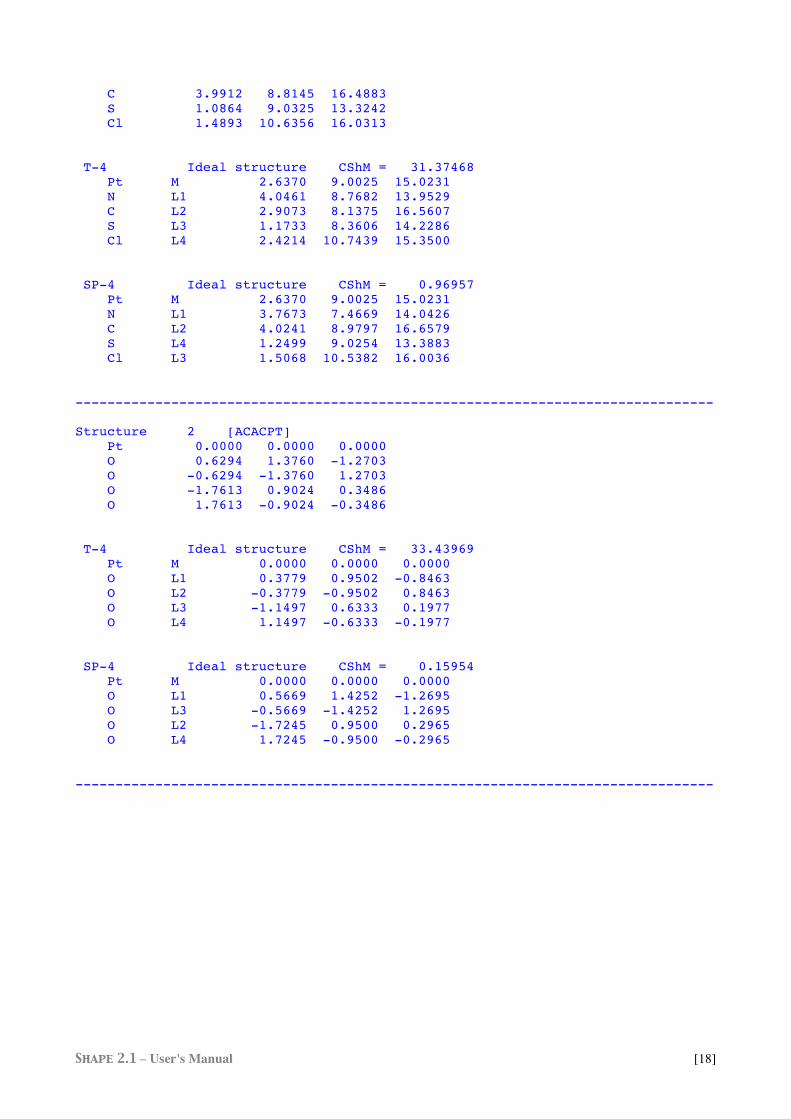
Output files: example04.tab (see example01.tab) and example04.out: -------------------------------------------------------------------------------- S H A P E v2.1 Continuous Shape Measures calculation (c) 2013 Electronic Structure Group, Universitat de Barcelona Contact: [email protected] -------------------------------------------------------------------------------- Example 4: Four-coordinate complexes, %fullout option -------------------------------------------------------------------------------- Ideal structures ML4 T-4 2 Td Tetrahedron SP-4 1 D4h Square -------------------------------------------------------------------------------- Structure 1 [ABOXIY] Pt 2.7159 8.9642 15.0153 N 3.9023 7.5659 14.2563
Shape 2.1 – User's Manual [18]
C 3.9912 8.8145 16.4883 S 1.0864 9.0325 13.3242 Cl 1.4893 10.6356 16.0313 T-4 Ideal structure CShM = 31.37468 Pt M 2.6370 9.0025 15.0231 N L1 4.0461 8.7682 13.9529 C L2 2.9073 8.1375 16.5607 S L3 1.1733 8.3606 14.2286 Cl L4 2.4214 10.7439 15.3500 SP-4 Ideal structure CShM = 0.96957 Pt M 2.6370 9.0025 15.0231 N L1 3.7673 7.4669 14.0426 C L2 4.0241 8.9797 16.6579 S L4 1.2499 9.0254 13.3883 Cl L3 1.5068 10.5382 16.0036 -------------------------------------------------------------------------------- Structure 2 [ACACPT] Pt 0.0000 0.0000 0.0000 O 0.6294 1.3760 -1.2703 O -0.6294 -1.3760 1.2703 O -1.7613 0.9024 0.3486 O 1.7613 -0.9024 -0.3486 T-4 Ideal structure CShM = 33.43969 Pt M 0.0000 0.0000 0.0000 O L1 0.3779 0.9502 -0.8463 O L2 -0.3779 -0.9502 0.8463 O L3 -1.1497 0.6333 0.1977 O L4 1.1497 -0.6333 -0.1977 SP-4 Ideal structure CShM = 0.15954 Pt M 0.0000 0.0000 0.0000 O L1 0.5669 1.4252 -1.2695 O L3 -0.5669 -1.4252 1.2695 O L2 -1.7245 0.9500 0.2965 O L4 1.7245 -0.9500 -0.2965 --------------------------------------------------------------------------------
Shape 2.1 – User's Manual [19]
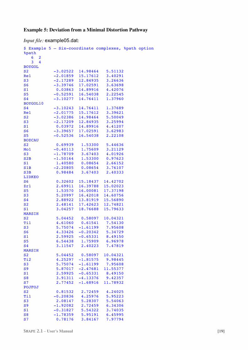
Example 5: Deviation from a Minimal Distortion Pathway
Input file: example05.dat: $ Example 5 – Six-coordinate complexes, %path option %path 6 2 3 4 BOYGOL S2 -3.02522 14.98464 5.51132 Re1 -2.01859 15.17612 3.40291 S3 -2.17289 12.84935 3.26636 S6 -3.39746 17.02591 3.63698 S1 0.03863 14.89916 4.42076 S5 -0.52591 16.54038 2.22545 S4 -3.10277 14.76411 1.37960 BOYGOL10 S4 -3.10243 14.76411 1.37689 Re1 -2.01775 15.17612 3.39621 S2 -3.02386 14.98464 5.50049 S3 -2.17209 12.84935 3.25994 S1 0.03972 14.89916 4.41207 S6 -3.39657 17.02591 3.62983 S5 -0.52536 16.54038 2.22108 BOZCAU S2 0.69939 1.53300 5.44636 Mo1 -0.40113 1.75609 3.21129 S3 -1.78709 3.67403 4.01926 S2B -1.50164 1.53300 0.97623 S1 1.40580 0.08654 2.66152 S1B -2.20805 0.08654 3.76107 S3B 0.98484 3.67403 2.40333 LIDKEO S6 0.32602 15.18437 14.42702 Zr1 2.69911 16.39788 15.02023 S5 1.53570 16.00081 17.37198 S3 5.20997 16.42018 14.60756 S4 2.88922 13.81919 15.56890 S2 2.48141 17.42623 12.74821 S1 3.04257 18.76688 15.79633 MARSIH S2 5.04452 0.58097 10.04321 Ti1 4.61060 0.61541 7.54130 S3 5.75074 -1.61199 7.95608 S6 4.33426 -0.20342 5.34729 S1 2.59925 -0.65331 8.49150 S5 6.54438 1.75909 6.96978 S4 3.11547 2.40223 7.47819 MARSIH S2 5.04452 0.58097 10.04321 Ti2 4.25297 -1.81575 9.98445 S3 5.75074 -1.61199 7.95608 S9 5.87017 -2.47681 11.55377 S1 2.59925 -0.65331 8.49150 S8 3.91311 -4.13376 9.42357 S7 2.77452 -1.68916 11.78932 POJFOJ S2 0.81532 2.72459 4.24025 Ti1 -0.20836 4.25976 5.95223 S3 2.08147 5.28307 5.54063 S9 -1.92082 2.72459 6.34306 S1 -0.31827 5.54322 3.74035 S8 -1.78359 5.95191 6.45995 S7 0.78176 3.84167 7.97794
Shape 2.1 – User's Manual [20]
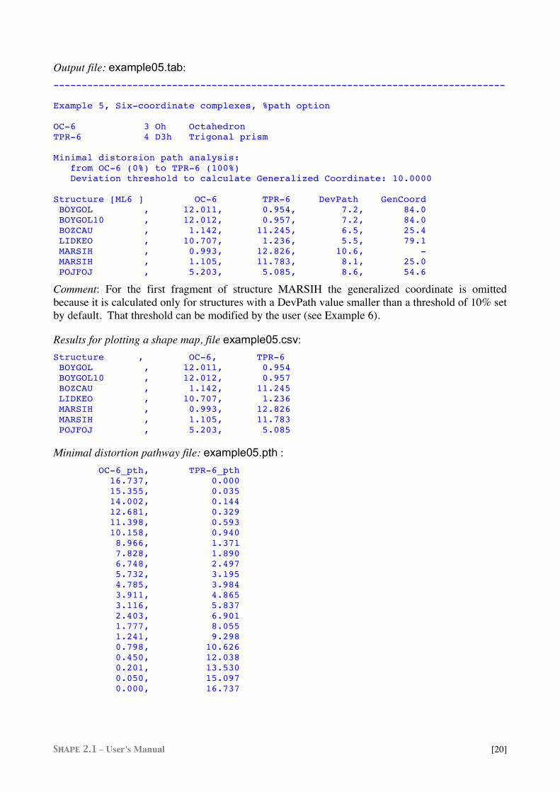
Output file: example05.tab: -------------------------------------------------------------------------------- Example 5, Six-coordinate complexes, %path option OC-6 3 Oh Octahedron TPR-6 4 D3h Trigonal prism Minimal distorsion path analysis: from OC-6 (0%) to TPR-6 (100%) Deviation threshold to calculate Generalized Coordinate: 10.0000 Structure [ML6 ] OC-6 TPR-6 DevPath GenCoord BOYGOL , 12.011, 0.954, 7.2, 84.0 BOYGOL10 , 12.012, 0.957, 7.2, 84.0 BOZCAU , 1.142, 11.245, 6.5, 25.4 LIDKEO , 10.707, 1.236, 5.5, 79.1 MARSIH , 0.993, 12.826, 10.6, - MARSIH , 1.105, 11.783, 8.1, 25.0 POJFOJ , 5.203, 5.085, 8.6, 54.6
Comment: For the first fragment of structure MARSIH the generalized coordinate is omitted because it is calculated only for structures with a DevPath value smaller than a threshold of 10% set by default. That threshold can be modified by the user (see Example 6).
Results for plotting a shape map, file example05.csv: Structure , OC-6, TPR-6 BOYGOL , 12.011, 0.954 BOYGOL10 , 12.012, 0.957 BOZCAU , 1.142, 11.245 LIDKEO , 10.707, 1.236 MARSIH , 0.993, 12.826 MARSIH , 1.105, 11.783 POJFOJ , 5.203, 5.085
Minimal distortion pathway file: example05.pth : OC-6_pth, TPR-6_pth 16.737, 0.000 15.355, 0.035 14.002, 0.144 12.681, 0.329 11.398, 0.593 10.158, 0.940 8.966, 1.371 7.828, 1.890 6.748, 2.497 5.732, 3.195 4.785, 3.984 3.911, 4.865 3.116, 5.837 2.403, 6.901 1.777, 8.055 1.241, 9.298 0.798, 10.626 0.450, 12.038 0.201, 13.530 0.050, 15.097 0.000, 16.737
Shape 2.1 – User's Manual [21]
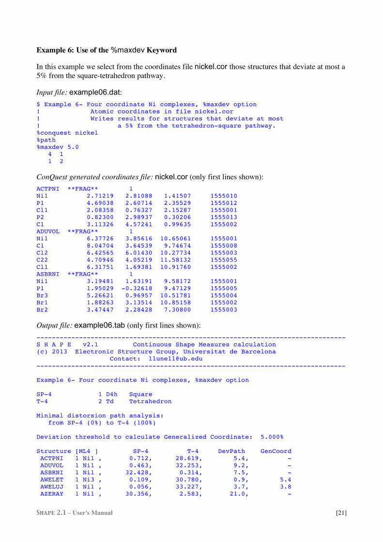
Example 6: Use of the %maxdev Keyword
In this example we select from the coordinates file nickel.cor those structures that deviate at most a 5% from the square-tetrahedron pathway.
Input file: example06.dat: $ Example 6- Four coordinate Ni complexes, %maxdev option ! Atomic coordinates in file nickel.cor ! Writes results for structures that deviate at most ! a 5% from the tetrahedron-square pathway. %conquest nickel %path %maxdev 5.0 4 1 1 2
ConQuest generated coordinates file: nickel.cor (only first lines shown): ACTPNI **FRAG** 1 Ni1 2.71219 2.81088 1.41507 1555010 P1 4.69038 2.60714 2.35529 1555012 Cl1 2.08358 0.76327 2.15287 1555001 P2 0.82300 2.98937 0.30206 1555013 C1 3.11326 4.57241 0.99635 1555002 ADUVOL **FRAG** 1 Ni1 6.37726 3.85616 10.65061 1555001 C1 8.04704 3.64539 9.74674 1555008 Cl2 6.42565 6.01430 10.27734 1555003 C22 4.70946 4.05219 11.58132 1555055 Cl1 6.31751 1.69381 10.91760 1555002 ASBRNI **FRAG** 1 Ni1 3.19481 1.63191 9.58172 1555001 P1 1.95029 -0.32618 9.47129 1555005 Br3 5.26621 0.96957 10.51781 1555004 Br1 1.88263 3.13514 10.85158 1555002 Br2 3.47447 2.28428 7.30800 1555003
Output file: example06.tab (only first lines shown): -------------------------------------------------------------------------------- S H A P E v2.1 Continuous Shape Measures calculation (c) 2013 Electronic Structure Group, Universitat de Barcelona Contact: [email protected] -------------------------------------------------------------------------------- Example 6- Four coordinate Ni complexes, %maxdev option SP-4 1 D4h Square T-4 2 Td Tetrahedron Minimal distorsion path analysis: from SP-4 (0%) to T-4 (100%) Deviation threshold to calculate Generalized Coordinate: 5.000% Structure [ML4 ] SP-4 T-4 DevPath GenCoord ACTPNI 1 Ni1 , 0.712, 28.619, 5.4, - ADUVOL 1 Ni1 , 0.463, 32.253, 9.2, - ASBRNI 1 Ni1 , 32.428, 0.314, 7.5, - AWELET 1 Ni3 , 0.109, 30.780, 0.9, 5.4 AWELUJ 1 Ni1 , 0.056, 33.227, 3.7, 3.8 AZERAY 1 Ni1 , 30.356, 2.583, 21.0, -
Shape 2.1 – User's Manual [22]
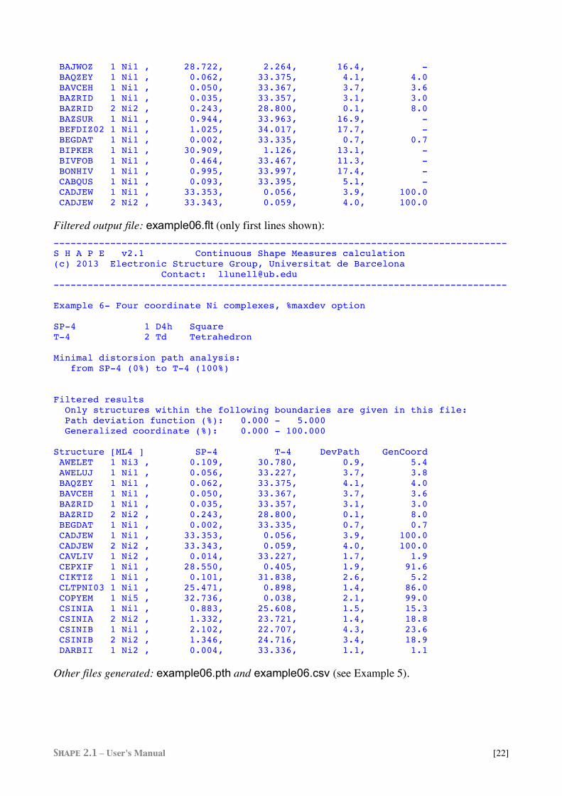
BAJWOZ 1 Ni1 , 28.722, 2.264, 16.4, - BAQZEY 1 Ni1 , 0.062, 33.375, 4.1, 4.0 BAVCEH 1 Ni1 , 0.050, 33.367, 3.7, 3.6 BAZRID 1 Ni1 , 0.035, 33.357, 3.1, 3.0 BAZRID 2 Ni2 , 0.243, 28.800, 0.1, 8.0 BAZSUR 1 Ni1 , 0.944, 33.963, 16.9, - BEFDIZ02 1 Ni1 , 1.025, 34.017, 17.7, - BEGDAT 1 Ni1 , 0.002, 33.335, 0.7, 0.7 BIPKER 1 Ni1 , 30.909, 1.126, 13.1, - BIVFOB 1 Ni1 , 0.464, 33.467, 11.3, - BONHIV 1 Ni1 , 0.995, 33.997, 17.4, - CABQUS 1 Ni1 , 0.093, 33.395, 5.1, - CADJEW 1 Ni1 , 33.353, 0.056, 3.9, 100.0 CADJEW 2 Ni2 , 33.343, 0.059, 4.0, 100.0
Filtered output file: example06.flt (only first lines shown): -------------------------------------------------------------------------------- S H A P E v2.1 Continuous Shape Measures calculation (c) 2013 Electronic Structure Group, Universitat de Barcelona Contact: [email protected] -------------------------------------------------------------------------------- Example 6- Four coordinate Ni complexes, %maxdev option SP-4 1 D4h Square T-4 2 Td Tetrahedron Minimal distorsion path analysis: from SP-4 (0%) to T-4 (100%) Filtered results Only structures within the following boundaries are given in this file: Path deviation function (%): 0.000 - 5.000 Generalized coordinate (%): 0.000 - 100.000 Structure [ML4 ] SP-4 T-4 DevPath GenCoord AWELET 1 Ni3 , 0.109, 30.780, 0.9, 5.4 AWELUJ 1 Ni1 , 0.056, 33.227, 3.7, 3.8 BAQZEY 1 Ni1 , 0.062, 33.375, 4.1, 4.0 BAVCEH 1 Ni1 , 0.050, 33.367, 3.7, 3.6 BAZRID 1 Ni1 , 0.035, 33.357, 3.1, 3.0 BAZRID 2 Ni2 , 0.243, 28.800, 0.1, 8.0 BEGDAT 1 Ni1 , 0.002, 33.335, 0.7, 0.7 CADJEW 1 Ni1 , 33.353, 0.056, 3.9, 100.0 CADJEW 2 Ni2 , 33.343, 0.059, 4.0, 100.0 CAVLIV 1 Ni2 , 0.014, 33.227, 1.7, 1.9 CEPXIF 1 Ni1 , 28.550, 0.405, 1.9, 91.6 CIKTIZ 1 Ni1 , 0.101, 31.838, 2.6, 5.2 CLTPNI03 1 Ni1 , 25.471, 0.898, 1.4, 86.0 COPYEM 1 Ni5 , 32.736, 0.038, 2.1, 99.0 CSINIA 1 Ni1 , 0.883, 25.608, 1.5, 15.3 CSINIA 2 Ni2 , 1.332, 23.721, 1.4, 18.8 CSINIB 1 Ni1 , 2.102, 22.707, 4.3, 23.6 CSINIB 2 Ni2 , 1.346, 24.716, 3.4, 18.9 DARBII 1 Ni2 , 0.004, 33.336, 1.1, 1.1
Other files generated: example06.pth and example06.csv (see Example 5).
Shape 2.1 – User's Manual [23]
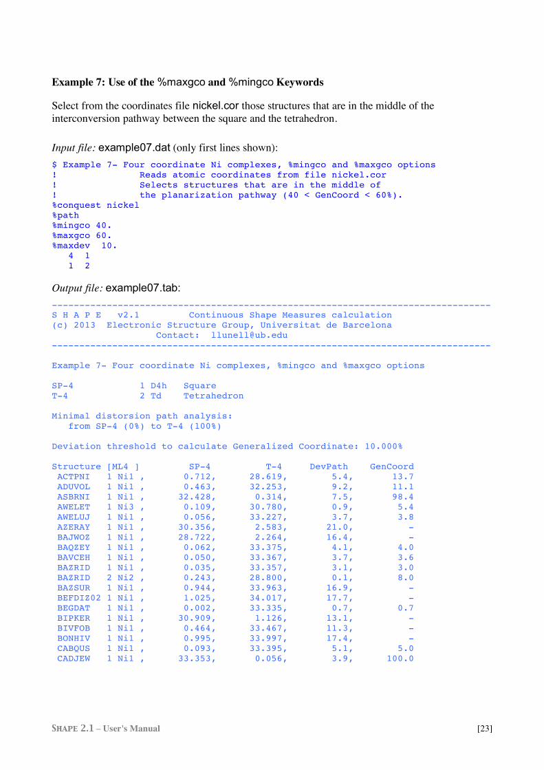
Example 7: Use of the %maxgco and %mingco Keywords
Select from the coordinates file nickel.cor those structures that are in the middle of the interconversion pathway between the square and the tetrahedron.
Input file: example07.dat (only first lines shown): $ Example 7- Four coordinate Ni complexes, %mingco and %maxgco options ! Reads atomic coordinates from file nickel.cor ! Selects structures that are in the middle of ! the planarization pathway (40 < GenCoord < 60%). %conquest nickel %path %mingco 40. %maxgco 60. %maxdev 10. 4 1 1 2
Output file: example07.tab: -------------------------------------------------------------------------------- S H A P E v2.1 Continuous Shape Measures calculation (c) 2013 Electronic Structure Group, Universitat de Barcelona Contact: [email protected] -------------------------------------------------------------------------------- Example 7- Four coordinate Ni complexes, %mingco and %maxgco options SP-4 1 D4h Square T-4 2 Td Tetrahedron Minimal distorsion path analysis: from SP-4 (0%) to T-4 (100%) Deviation threshold to calculate Generalized Coordinate: 10.000% Structure [ML4 ] SP-4 T-4 DevPath GenCoord ACTPNI 1 Ni1 , 0.712, 28.619, 5.4, 13.7 ADUVOL 1 Ni1 , 0.463, 32.253, 9.2, 11.1 ASBRNI 1 Ni1 , 32.428, 0.314, 7.5, 98.4 AWELET 1 Ni3 , 0.109, 30.780, 0.9, 5.4 AWELUJ 1 Ni1 , 0.056, 33.227, 3.7, 3.8 AZERAY 1 Ni1 , 30.356, 2.583, 21.0, - BAJWOZ 1 Ni1 , 28.722, 2.264, 16.4, - BAQZEY 1 Ni1 , 0.062, 33.375, 4.1, 4.0 BAVCEH 1 Ni1 , 0.050, 33.367, 3.7, 3.6 BAZRID 1 Ni1 , 0.035, 33.357, 3.1, 3.0 BAZRID 2 Ni2 , 0.243, 28.800, 0.1, 8.0 BAZSUR 1 Ni1 , 0.944, 33.963, 16.9, - BEFDIZ02 1 Ni1 , 1.025, 34.017, 17.7, - BEGDAT 1 Ni1 , 0.002, 33.335, 0.7, 0.7 BIPKER 1 Ni1 , 30.909, 1.126, 13.1, - BIVFOB 1 Ni1 , 0.464, 33.467, 11.3, - BONHIV 1 Ni1 , 0.995, 33.997, 17.4, - CABQUS 1 Ni1 , 0.093, 33.395, 5.1, 5.0 CADJEW 1 Ni1 , 33.353, 0.056, 3.9, 100.0
Shape 2.1 – User's Manual [24]
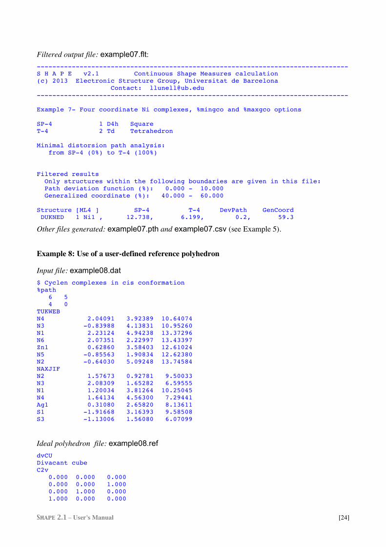
Filtered output file: example07.flt: -------------------------------------------------------------------------------- S H A P E v2.1 Continuous Shape Measures calculation (c) 2013 Electronic Structure Group, Universitat de Barcelona Contact: [email protected] -------------------------------------------------------------------------------- Example 7- Four coordinate Ni complexes, %mingco and %maxgco options SP-4 1 D4h Square T-4 2 Td Tetrahedron Minimal distorsion path analysis: from SP-4 (0%) to T-4 (100%) Filtered results Only structures within the following boundaries are given in this file: Path deviation function (%): 0.000 - 10.000 Generalized coordinate (%): 40.000 - 60.000 Structure [ML4 ] SP-4 T-4 DevPath GenCoord DUKNED 1 Ni1 , 12.738, 6.199, 0.2, 59.3
Other files generated: example07.pth and example07.csv (see Example 5).
Example 8: Use of a user-defined reference polyhedron
Input file: example08.dat $ Cyclen complexes in cis conformation %path 6 5 4 0 TUKWEB N4 2.04091 3.92389 10.64074 N3 -0.83988 4.13831 10.95260 N1 2.23124 4.94238 13.37296 N6 2.07351 2.22997 13.43397 Zn1 0.62860 3.58403 12.61024 N5 -0.85563 1.90834 12.62380 N2 -0.64030 5.09248 13.74584 NAXJIF N2 1.57673 0.92781 9.50033 N3 2.08309 1.65282 6.59555 N1 1.20034 3.81264 10.25045 N4 1.64134 4.56300 7.29441 Ag1 0.31080 2.65820 8.13611 S1 -1.91668 3.16393 9.58508 S3 -1.13006 1.56080 6.07099
Ideal polyhedron file: example08.ref dvCU Divacant cube C2v 0.000 0.000 0.000 0.000 0.000 1.000 0.000 1.000 0.000 1.000 0.000 0.000
Shape 2.1 – User's Manual [25]
1.000 1.000 0.000 1.000 1.000 1.000 0.500 0.500 0.500
Note that in the .ref file the coordinates of the central atom must be in the last line.
Alternatively one could use an ideal polyhedron file dvcube.ide introducing the %ideal dvcube instruction in the input file.
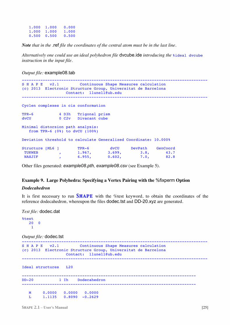
Output file: example08.tab -------------------------------------------------------------------------------- S H A P E v2.1 Continuous Shape Measures calculation (c) 2013 Electronic Structure Group, Universitat de Barcelona Contact: [email protected] -------------------------------------------------------------------------------- Cyclen complexes in cis conformation TPR-6 4 D3h Trigonal prism dvCU 0 C2v Divacant cube Minimal distorsion path analysis: from TPR-6 (0%) to dvCU (100%) Deviation threshold to calculate Generalized Coordinate: 10.000% Structure [ML6 ] TPR-6 dvCU DevPath GenCoord TUKWEB , 1.967, 3.699, 3.8, 43.7 NAXJIF , 6.955, 0.602, 7.0, 82.8 Other files generated: example08.pth, example08.csv (see Example 5).
Example 9. Large Polyhedra: Specifying a Vertex Pairing with the %fixperm Option Dodecahedron
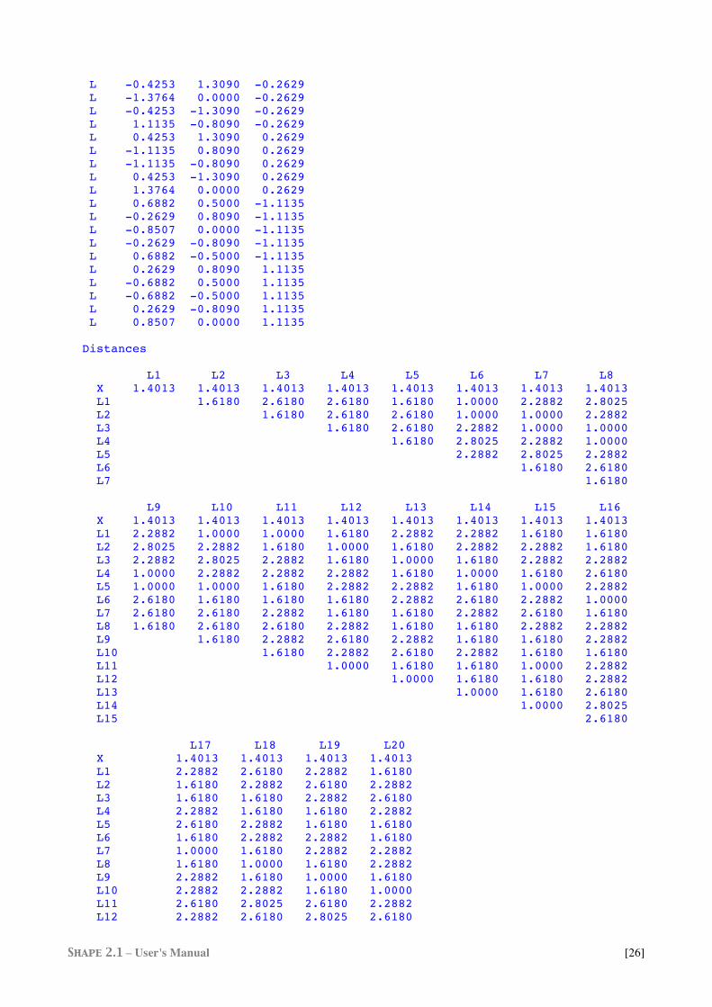
It is first necessary to run Shape with the %test keyword, to obtain the coordinates of the reference dodecahedron, whereupon the files dodec.tst and DD-20.xyz are generated.
Test file: dodec.dat %test 20 0 1
Output file: dodec.tst -------------------------------------------------------------------------------- S H A P E v2.1 Continuous Shape Measures calculation (c) 2013 Electronic Structure Group, Universitat de Barcelona Contact: [email protected] -------------------------------------------------------------------------------- Ideal structures L20 --------------------------------------------------------------------------- DD-20 1 Ih Dodecahedron --------------------------------------------------------------------------- M 0.0000 0.0000 0.0000 L 1.1135 0.8090 -0.2629
Shape 2.1 – User's Manual [26]
L -0.4253 1.3090 -0.2629 L -1.3764 0.0000 -0.2629 L -0.4253 -1.3090 -0.2629 L 1.1135 -0.8090 -0.2629 L 0.4253 1.3090 0.2629 L -1.1135 0.8090 0.2629 L -1.1135 -0.8090 0.2629 L 0.4253 -1.3090 0.2629 L 1.3764 0.0000 0.2629 L 0.6882 0.5000 -1.1135 L -0.2629 0.8090 -1.1135 L -0.8507 0.0000 -1.1135 L -0.2629 -0.8090 -1.1135 L 0.6882 -0.5000 -1.1135 L 0.2629 0.8090 1.1135 L -0.6882 0.5000 1.1135 L -0.6882 -0.5000 1.1135 L 0.2629 -0.8090 1.1135 L 0.8507 0.0000 1.1135 Distances L1 L2 L3 L4 L5 L6 L7 L8 X 1.4013 1.4013 1.4013 1.4013 1.4013 1.4013 1.4013 1.4013 L1 1.6180 2.6180 2.6180 1.6180 1.0000 2.2882 2.8025 L2 1.6180 2.6180 2.6180 1.0000 1.0000 2.2882 L3 1.6180 2.6180 2.2882 1.0000 1.0000 L4 1.6180 2.8025 2.2882 1.0000 L5 2.2882 2.8025 2.2882 L6 1.6180 2.6180 L7 1.6180 L9 L10 L11 L12 L13 L14 L15 L16 X 1.4013 1.4013 1.4013 1.4013 1.4013 1.4013 1.4013 1.4013 L1 2.2882 1.0000 1.0000 1.6180 2.2882 2.2882 1.6180 1.6180 L2 2.8025 2.2882 1.6180 1.0000 1.6180 2.2882 2.2882 1.6180 L3 2.2882 2.8025 2.2882 1.6180 1.0000 1.6180 2.2882 2.2882 L4 1.0000 2.2882 2.2882 2.2882 1.6180 1.0000 1.6180 2.6180 L5 1.0000 1.0000 1.6180 2.2882 2.2882 1.6180 1.0000 2.2882 L6 2.6180 1.6180 1.6180 1.6180 2.2882 2.6180 2.2882 1.0000 L7 2.6180 2.6180 2.2882 1.6180 1.6180 2.2882 2.6180 1.6180 L8 1.6180 2.6180 2.6180 2.2882 1.6180 1.6180 2.2882 2.2882 L9 1.6180 2.2882 2.6180 2.2882 1.6180 1.6180 2.2882 L10 1.6180 2.2882 2.6180 2.2882 1.6180 1.6180 L11 1.0000 1.6180 1.6180 1.0000 2.2882 L12 1.0000 1.6180 1.6180 2.2882 L13 1.0000 1.6180 2.6180 L14 1.0000 2.8025 L15 2.6180 L17 L18 L19 L20 X 1.4013 1.4013 1.4013 1.4013 L1 2.2882 2.6180 2.2882 1.6180 L2 1.6180 2.2882 2.6180 2.2882 L3 1.6180 1.6180 2.2882 2.6180 L4 2.2882 1.6180 1.6180 2.2882 L5 2.6180 2.2882 1.6180 1.6180 L6 1.6180 2.2882 2.2882 1.6180 L7 1.0000 1.6180 2.2882 2.2882 L8 1.6180 1.0000 1.6180 2.2882 L9 2.2882 1.6180 1.0000 1.6180 L10 2.2882 2.2882 1.6180 1.0000 L11 2.6180 2.8025 2.6180 2.2882 L12 2.2882 2.6180 2.8025 2.6180
Shape 2.1 – User's Manual [27]
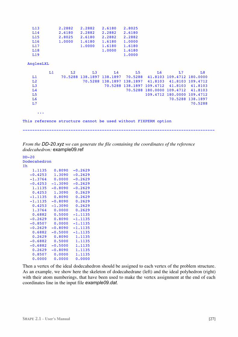
L13 2.2882 2.2882 2.6180 2.8025 L14 2.6180 2.2882 2.2882 2.6180 L15 2.8025 2.6180 2.2882 2.2882 L16 1.0000 1.6180 1.6180 1.0000 L17 1.0000 1.6180 1.6180 L18 1.0000 1.6180 L19 1.0000 AnglesLXL L1 L2 L3 L4 L5 L6 L7 L8 L1 70.5288 138.1897 138.1897 70.5288 41.8103 109.4712 180.0000 L2 70.5288 138.1897 138.1897 41.8103 41.8103 109.4712 L3 70.5288 138.1897 109.4712 41.8103 41.8103 L4 70.5288 180.0000 109.4712 41.8103 L5 109.4712 180.0000 109.4712 L6 70.5288 138.1897 L7 70.5288 ... This reference structure cannot be used without FIXPERM option --------------------------------------------------------------------------------
From the DD-20.xyz we can generate the file containing the coordinates of the reference dodecahedron: example09.ref DD-20 Dodecahedron Ih 1.1135 0.8090 -0.2629 -0.4253 1.3090 -0.2629 -1.3764 0.0000 -0.2629 -0.4253 -1.3090 -0.2629 1.1135 -0.8090 -0.2629 0.4253 1.3090 0.2629 -1.1135 0.8090 0.2629 -1.1135 -0.8090 0.2629 0.4253 -1.3090 0.2629 1.3764 0.0000 0.2629 0.6882 0.5000 -1.1135 -0.2629 0.8090 -1.1135 -0.8507 0.0000 -1.1135 -0.2629 -0.8090 -1.1135 0.6882 -0.5000 -1.1135 0.2629 0.8090 1.1135 -0.6882 0.5000 1.1135 -0.6882 -0.5000 1.1135 0.2629 -0.8090 1.1135 0.8507 0.0000 1.1135 0.0000 0.0000 0.0000
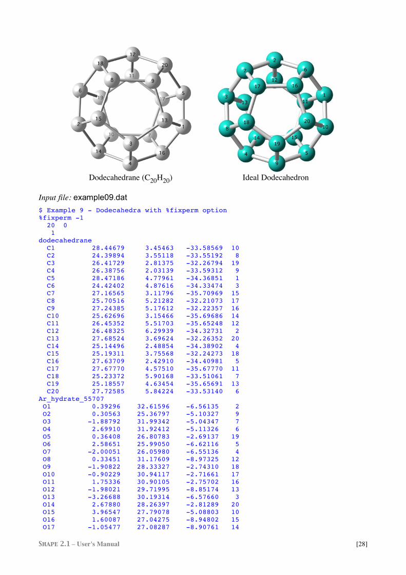
Then a vertex of the ideal dodecahedron should be assigned to each vertex of the problem structure. As an example, we show here the skeleton of dodecahedrane (left) and the ideal polyhedron (right) with their atom numberings, that have been used to make the vertex assignment at the end of each coordinates line in the input file example09.dat.
Shape 2.1 – User's Manual [28]
Dodecahedrane (C20H20) Ideal Dodecahedron
Input file: example09.dat $ Example 9 - Dodecahedra with %fixperm option %fixperm -1 20 0 1 dodecahedrane C1 28.44679 3.45463 -33.58569 10 C2 24.39894 3.55118 -33.55192 8 C3 26.41729 2.81375 -32.26794 19 C4 26.38756 2.03139 -33.59312 9 C5 28.47186 4.77961 -34.36851 1 C6 24.42402 4.87616 -34.33474 3 C7 27.16565 3.11796 -35.70969 15 C8 25.70516 5.21282 -32.21073 17 C9 27.24385 5.17612 -32.22357 16 C10 25.62696 3.15466 -35.69686 14 C11 26.45352 5.51703 -35.65248 12 C12 26.48325 6.29939 -34.32731 2 C13 27.68524 3.69624 -32.26352 20 C14 25.14496 2.48854 -34.38902 4 C15 25.19311 3.75568 -32.24273 18 C16 27.63709 2.42910 -34.40981 5 C17 27.67770 4.57510 -35.67770 11 C18 25.23372 5.90168 -33.51061 7 C19 25.18557 4.63454 -35.65691 13 C20 27.72585 5.84224 -33.53140 6 Ar_hydrate_55707 O1 0.39296 32.61596 -6.56135 2 O2 0.30563 25.36797 -5.10327 9 O3 -1.88792 31.99342 -5.04347 7 O4 2.69910 31.92412 -5.11326 6 O5 0.36408 26.80783 -2.69137 19 O6 2.58651 25.99050 -6.62116 5 O7 -2.00051 26.05980 -6.55136 4 O8 0.33451 31.17609 -8.97325 12 O9 -1.90822 28.33327 -2.74310 18 O10 -0.90229 30.94117 -2.71661 17 O11 1.75336 30.90105 -2.75702 16 O12 -1.98021 29.71995 -8.85174 13 O13 -3.26688 30.19314 -6.57660 3 O14 2.67880 28.26397 -2.81289 20 O15 3.96547 27.79078 -5.08803 10 O16 1.60087 27.04275 -8.94802 15 O17 -1.05477 27.08287 -8.90761 14
Shape 2.1 – User's Manual [29]
O18 3.97579 30.08372 -6.68680 1 O19 2.60681 29.65064 -8.92153 11 O20 -3.27720 27.90021 -4.97783 8
Output file: example09.tab -------------------------------------------------------------------------------- S H A P E v2.1 Continuous Shape Measures calculation (c) 2013 Electronic Structure Group, Universitat de Barcelona Contact: [email protected] -------------------------------------------------------------------------------- Example 9 - Dodecahedra with %fixperm option DD-20 1 Ih Dodecahedron Fixed vertices permutation used for CShM (specific permutation for each fragment) Structure [L20 ] DD-20 dodecahedrane , 0.000 Ar_hydrate_5570, 0.075
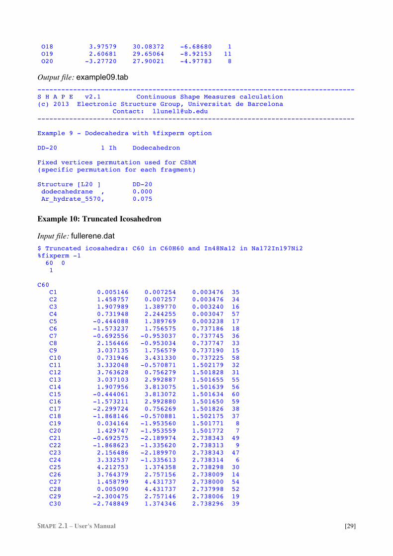
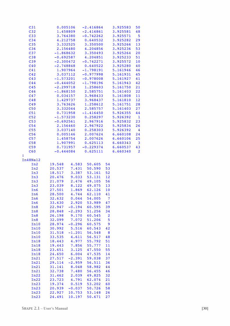
Example 10: Truncated Icosahedron
Input file: fullerene.dat $ Truncated icosahedra: C60 in C60H60 and In48Na12 in Na172In197Ni2 %fixperm -1 60 0 1 C60 C1 0.005146 0.007254 0.003476 35 C2 1.458757 0.007257 0.003476 34 C3 1.907989 1.389770 0.003240 16 C4 0.731948 2.244255 0.003047 57 C5 -0.444088 1.389769 0.003238 17 C6 -1.573237 1.756575 0.737186 18 C7 -0.692556 -0.953037 0.737745 36 C8 2.156466 -0.953034 0.737747 33 C9 3.037135 1.756579 0.737190 15 C10 0.731946 3.431330 0.737225 58 C11 3.332048 -0.570871 1.502179 32 C12 3.763628 0.756279 1.501828 31 C13 3.037103 2.992887 1.501655 55 C14 1.907956 3.813075 1.501639 56 C15 -0.444061 3.813072 1.501634 60 C16 -1.573211 2.992880 1.501650 59 C17 -2.299724 0.756269 1.501826 38 C18 -1.868146 -0.570881 1.502175 37 C19 0.034164 -1.953560 1.501771 8 C20 1.429747 -1.953559 1.501772 7 C21 -0.692575 -2.189974 2.738343 49 C22 -1.868623 -1.335620 2.738313 9 C23 2.156486 -2.189970 2.738343 47 C24 3.332537 -1.335613 2.738314 6 C25 4.212753 1.374358 2.738298 30 C26 3.764379 2.757156 2.738009 14 C27 1.458799 4.431737 2.738000 54 C28 0.005090 4.431737 2.737998 52 C29 -2.300475 2.757146 2.738006 19 C30 -2.748849 1.374346 2.738296 39
Shape 2.1 – User's Manual [30]
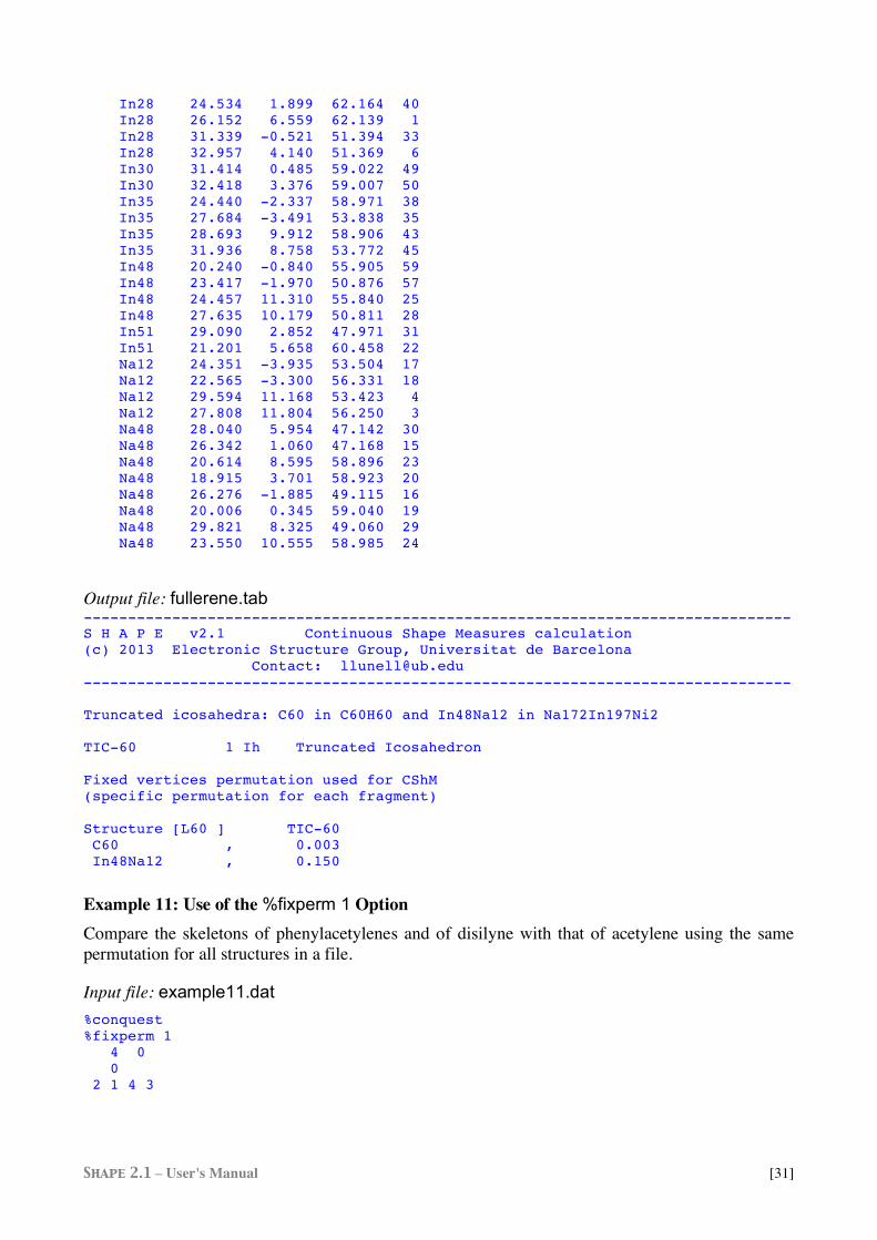
C31 0.005106 -2.416864 3.925583 50 C32 1.458809 -2.416861 3.925581 48 C33 3.764380 -0.742262 3.925571 5 C34 4.212758 0.640532 3.925282 29 C35 3.332525 3.350500 3.925266 13 C36 2.156480 4.204856 3.925236 53 C37 -1.868632 3.350493 3.925264 20 C38 -0.692587 4.204851 3.925233 51 C39 -2.300472 -0.742271 3.925572 10 C40 -2.748848 0.640522 3.925280 40 C41 1.907964 -1.798191 5.161946 46 C42 3.037112 -0.977998 5.161931 45 C43 -1.573201 -0.978008 5.161927 41 C44 -0.444052 -1.798196 5.161943 42 C45 -2.299718 1.258603 5.161750 21 C46 -1.868150 2.585751 5.161403 22 C47 0.034157 3.968433 5.161808 11 C48 1.429737 3.968437 5.161810 12 C49 3.763626 1.258612 5.161751 28 C50 3.332044 2.585757 5.161403 27 C51 0.731958 -1.416450 5.926355 44 C52 -1.573230 0.258297 5.926392 1 C53 -0.692561 2.967916 5.925832 23 C54 2.156460 2.967922 5.925834 26 C55 3.037140 0.258303 5.926392 4 C56 0.005146 2.007624 6.660108 24 C57 1.458754 2.007626 6.660106 25 C58 1.907991 0.625113 6.660343 3 C59 0.731957 -0.229374 6.660537 43 C60 -0.444084 0.625111 6.660340 2 ! In48Na12 In2 19.548 4.583 50.605 54 In2 20.537 7.431 50.590 53 In3 18.517 3.387 53.161 52 In3 20.476 9.033 53.131 12 In3 21.079 2.476 49.105 56 In3 23.039 8.122 49.075 13 In6 27.501 1.869 62.126 10 In6 28.500 4.744 62.110 41 In6 32.632 0.044 54.005 7 In6 33.630 2.920 53.989 47 In8 22.947 -0.194 60.595 39 In8 28.848 -2.293 51.256 34 In8 26.198 9.170 60.545 2 In8 32.099 7.072 51.206 5 In10 28.974 -0.296 60.575 9 In10 30.992 5.516 60.543 42 In10 31.518 -1.201 56.548 8 In10 33.535 4.611 56.517 48 In18 18.443 4.977 55.792 51 In18 19.443 7.856 55.777 11 In18 23.651 3.125 47.550 55 In18 24.650 6.004 47.535 14 In21 27.517 -2.391 59.038 37 In21 29.114 -2.959 56.511 36 In21 31.141 8.048 58.982 44 In21 32.738 7.480 56.455 46 In22 31.462 2.039 49.825 32 In22 23.723 4.791 62.074 21 In23 19.374 0.519 53.202 60 In23 20.939 -0.037 50.726 58 In23 22.927 10.753 53.148 26 In23 24.491 10.197 50.671 27
Shape 2.1 – User's Manual [31]
In28 24.534 1.899 62.164 40 In28 26.152 6.559 62.139 1 In28 31.339 -0.521 51.394 33 In28 32.957 4.140 51.369 6 In30 31.414 0.485 59.022 49 In30 32.418 3.376 59.007 50 In35 24.440 -2.337 58.971 38 In35 27.684 -3.491 53.838 35 In35 28.693 9.912 58.906 43 In35 31.936 8.758 53.772 45 In48 20.240 -0.840 55.905 59 In48 23.417 -1.970 50.876 57 In48 24.457 11.310 55.840 25 In48 27.635 10.179 50.811 28 In51 29.090 2.852 47.971 31 In51 21.201 5.658 60.458 22 Na12 24.351 -3.935 53.504 17 Na12 22.565 -3.300 56.331 18 Na12 29.594 11.168 53.423 4 Na12 27.808 11.804 56.250 3 Na48 28.040 5.954 47.142 30 Na48 26.342 1.060 47.168 15 Na48 20.614 8.595 58.896 23 Na48 18.915 3.701 58.923 20 Na48 26.276 -1.885 49.115 16 Na48 20.006 0.345 59.040 19 Na48 29.821 8.325 49.060 29 Na48 23.550 10.555 58.985 24
Output file: fullerene.tab -------------------------------------------------------------------------------- S H A P E v2.1 Continuous Shape Measures calculation (c) 2013 Electronic Structure Group, Universitat de Barcelona Contact: [email protected] -------------------------------------------------------------------------------- Truncated icosahedra: C60 in C60H60 and In48Na12 in Na172In197Ni2 TIC-60 1 Ih Truncated Icosahedron Fixed vertices permutation used for CShM (specific permutation for each fragment) Structure [L60 ] TIC-60 C60 , 0.003 In48Na12 , 0.150
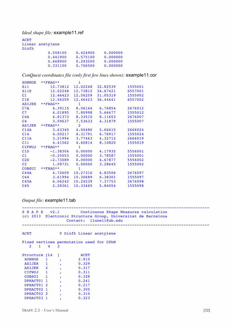
Example 11: Use of the %fixperm 1 Option Compare the skeletons of phenylacetylenes and of disilyne with that of acetylene using the same permutation for all structures in a file.
Input file: example11.dat %conquest %fixperm 1 4 0 0 2 1 4 3
Shape 2.1 – User's Manual [32]
Ideal shape file: example11.ref ACET Linear acetylene Dinfh 0.558100 0.424900 0.000000 0.441900 0.575100 0.000000 0.668900 0.293500 0.000000 0.331100 0.706500 0.000000
ConQuest coordinates file (only first few lines shown): example11.cor XONNOE **FRAG** 1 Si1 12.73812 12.02248 32.82539 1555001 Si1E 12.02248 12.73812 34.67421 6557001 C1 12.46423 12.56259 31.05319 1555002 C1E 12.56259 12.46423 36.44641 6557002 ASIJER **FRAG** 1 C7A 4.39115 8.06144 6.76854 2676012 C7 4.01895 7.80998 5.66677 1555012 C4A 4.81373 8.33510 8.11653 2676007 C4 3.59637 7.53633 4.31879 1555007 ASIJER **FRAG** 2 C14A 3.63340 4.06486 5.66615 2666024 C14 4.00217 4.31791 6.76917 1555024 C11A 3.21994 3.77463 4.32712 2666019 C11 4.41562 4.60814 8.10820 1555019 CIFWUJ **FRAG** 1 C1D -1.38304 0.00000 4.17935 5556001 C1 -0.25053 0.00000 3.78587 1555001 C2D -2.73089 0.00000 4.67877 5556002 C2 1.09731 0.00000 3.28645 1555002 COBSUI **FRAG** 1 C44A 4.72609 10.27316 6.83506 2676097 C44 3.61994 10.30689 6.38301 1555097 C45A 6.06242 10.24539 7.37753 2676098 C45 2.28361 10.33465 5.84054 1555098
Output file: example11.tab -------------------------------------------------------------------------------- S H A P E v2.1 Continuous Shape Measures calculation (c) 2013 Electronic Structure Group, Universitat de Barcelona Contact: [email protected] -------------------------------------------------------------------------------- ACET 0 Dinfh Linear acetylene Fixed vertices permutation used for CShM 2 1 4 3 Structure [L4 ] ACET XONNOE 1 , 2.915 ASIJER 1 , 0.329 ASIJER 2 , 0.317 CIFWUJ 1 , 0.311 COBSUI 1 , 0.328 DPHACT01 1 , 0.241 DPHACT01 2 , 0.217 DPHACT02 1 , 0.305 DPHACT02 2 , 0.310 DPHACT03 1 , 0.323
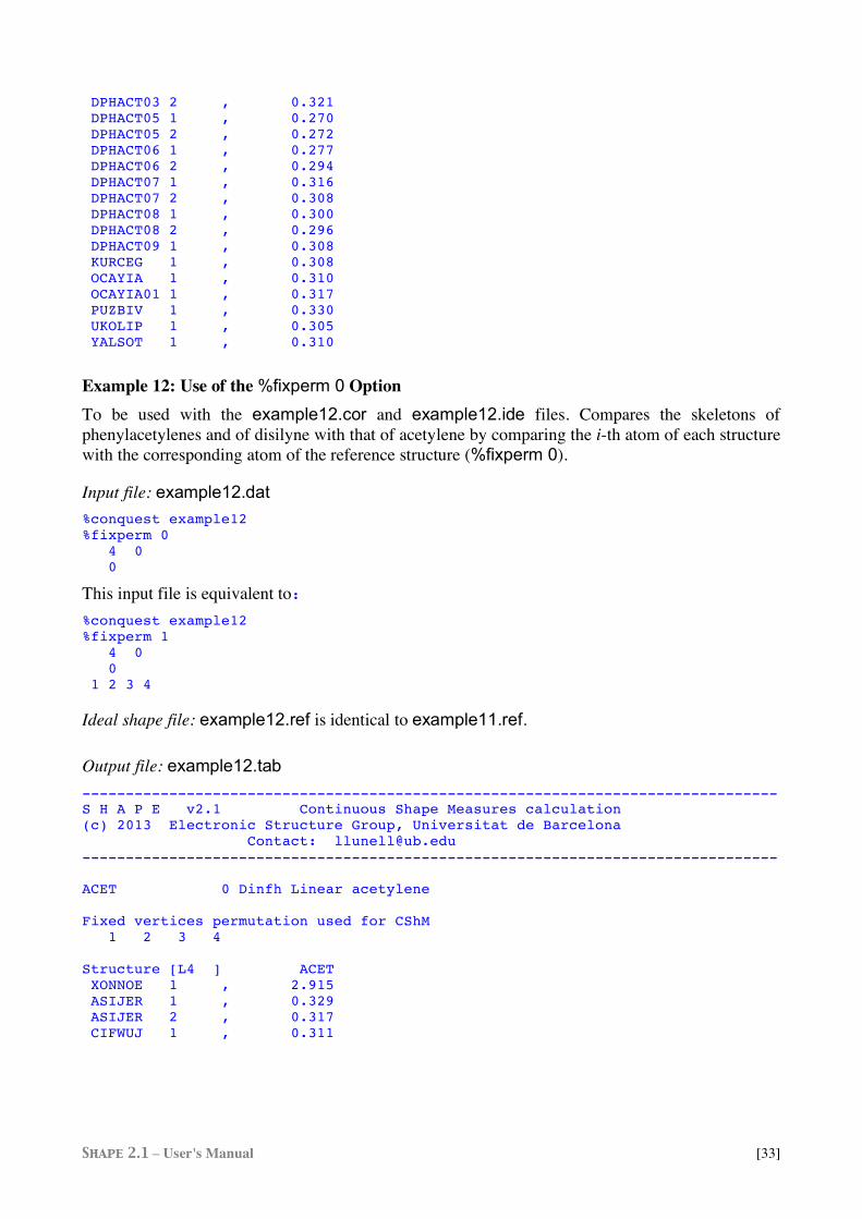
Shape 2.1 – User's Manual [33]
DPHACT03 2 , 0.321 DPHACT05 1 , 0.270 DPHACT05 2 , 0.272 DPHACT06 1 , 0.277 DPHACT06 2 , 0.294 DPHACT07 1 , 0.316 DPHACT07 2 , 0.308 DPHACT08 1 , 0.300 DPHACT08 2 , 0.296 DPHACT09 1 , 0.308 KURCEG 1 , 0.308 OCAYIA 1 , 0.310 OCAYIA01 1 , 0.317 PUZBIV 1 , 0.330 UKOLIP 1 , 0.305 YALSOT 1 , 0.310
Example 12: Use of the %fixperm 0 Option To be used with the example12.cor and example12.ide files. Compares the skeletons of phenylacetylenes and of disilyne with that of acetylene by comparing the i-th atom of each structure with the corresponding atom of the reference structure (%fixperm 0).
Input file: example12.dat %conquest example12 %fixperm 0 4 0 0
This input file is equivalent to: %conquest example12 %fixperm 1 4 0 0 1 2 3 4
Ideal shape file: example12.ref is identical to example11.ref.
Output file: example12.tab -------------------------------------------------------------------------------- S H A P E v2.1 Continuous Shape Measures calculation (c) 2013 Electronic Structure Group, Universitat de Barcelona Contact: [email protected] -------------------------------------------------------------------------------- ACET 0 Dinfh Linear acetylene Fixed vertices permutation used for CShM 1 2 3 4 Structure [L4 ] ACET XONNOE 1 , 2.915 ASIJER 1 , 0.329 ASIJER 2 , 0.317 CIFWUJ 1 , 0.311
Shape 2.1 – User's Manual [34]
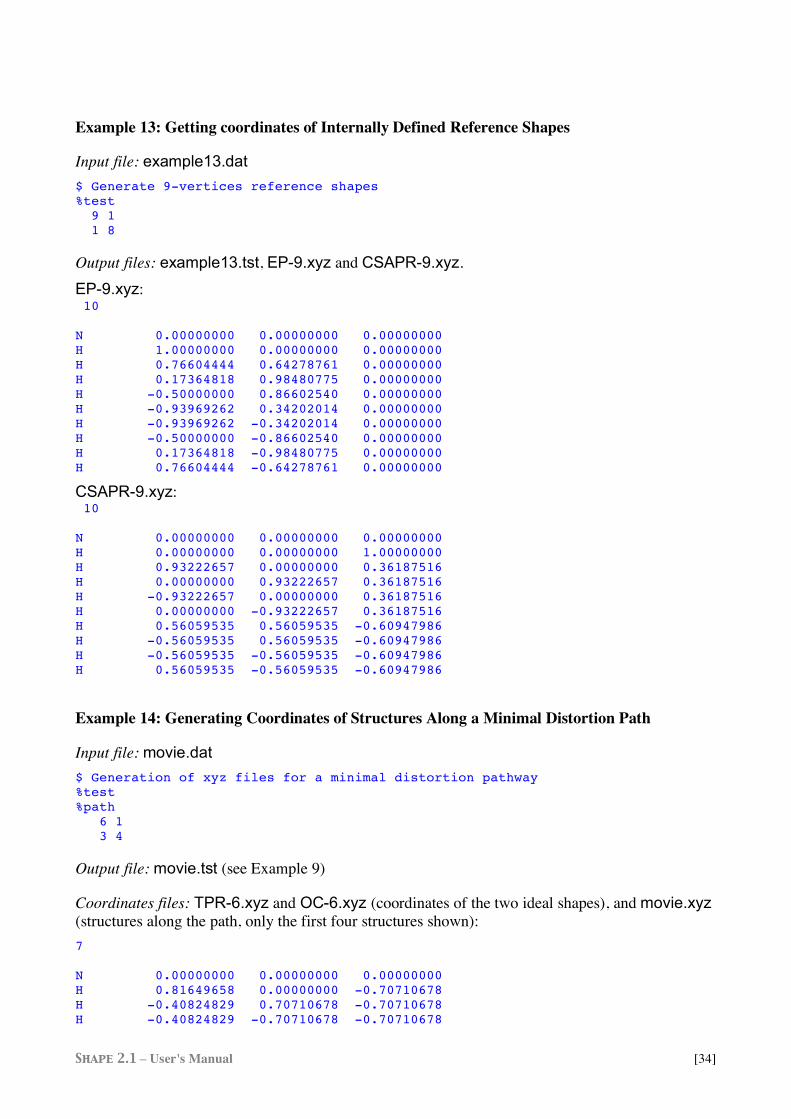
Example 13: Getting coordinates of Internally Defined Reference Shapes
Input file: example13.dat $ Generate 9-vertices reference shapes %test 9 1 1 8
Output files: example13.tst, EP-9.xyz and CSAPR-9.xyz. EP-9.xyz: 10 N 0.00000000 0.00000000 0.00000000 H 1.00000000 0.00000000 0.00000000 H 0.76604444 0.64278761 0.00000000 H 0.17364818 0.98480775 0.00000000 H -0.50000000 0.86602540 0.00000000 H -0.93969262 0.34202014 0.00000000 H -0.93969262 -0.34202014 0.00000000 H -0.50000000 -0.86602540 0.00000000 H 0.17364818 -0.98480775 0.00000000 H 0.76604444 -0.64278761 0.00000000
CSAPR-9.xyz: 10 N 0.00000000 0.00000000 0.00000000 H 0.00000000 0.00000000 1.00000000 H 0.93222657 0.00000000 0.36187516 H 0.00000000 0.93222657 0.36187516 H -0.93222657 0.00000000 0.36187516 H 0.00000000 -0.93222657 0.36187516 H 0.56059535 0.56059535 -0.60947986 H -0.56059535 0.56059535 -0.60947986 H -0.56059535 -0.56059535 -0.60947986 H 0.56059535 -0.56059535 -0.60947986
Example 14: Generating Coordinates of Structures Along a Minimal Distortion Path
Input file: movie.dat $ Generation of xyz files for a minimal distortion pathway %test %path 6 1 3 4
Output file: movie.tst (see Example 9)
Coordinates files: TPR-6.xyz and OC-6.xyz (coordinates of the two ideal shapes), and movie.xyz (structures along the path, only the first four structures shown): 7 N 0.00000000 0.00000000 0.00000000 H 0.81649658 0.00000000 -0.70710678 H -0.40824829 0.70710678 -0.70710678 H -0.40824829 -0.70710678 -0.70710678
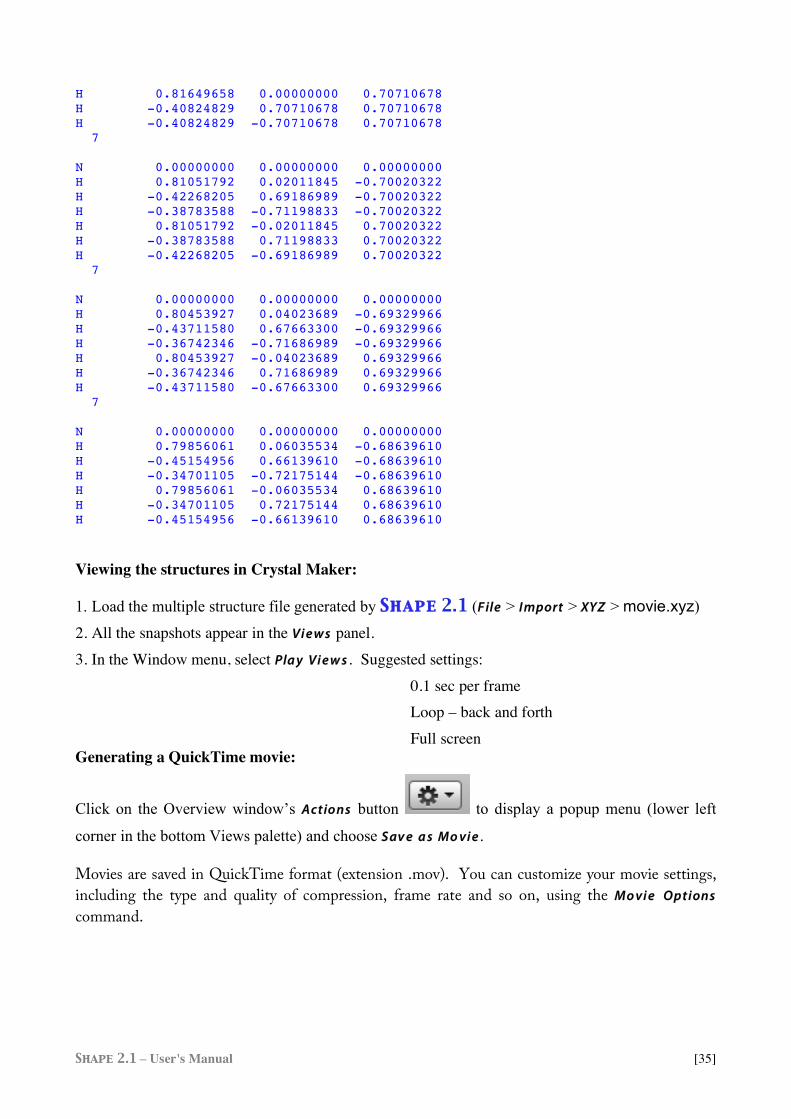
Shape 2.1 – User's Manual [35]
H 0.81649658 0.00000000 0.70710678 H -0.40824829 0.70710678 0.70710678 H -0.40824829 -0.70710678 0.70710678 7 N 0.00000000 0.00000000 0.00000000 H 0.81051792 0.02011845 -0.70020322 H -0.42268205 0.69186989 -0.70020322 H -0.38783588 -0.71198833 -0.70020322 H 0.81051792 -0.02011845 0.70020322 H -0.38783588 0.71198833 0.70020322 H -0.42268205 -0.69186989 0.70020322 7 N 0.00000000 0.00000000 0.00000000 H 0.80453927 0.04023689 -0.69329966 H -0.43711580 0.67663300 -0.69329966 H -0.36742346 -0.71686989 -0.69329966 H 0.80453927 -0.04023689 0.69329966 H -0.36742346 0.71686989 0.69329966 H -0.43711580 -0.67663300 0.69329966 7 N 0.00000000 0.00000000 0.00000000 H 0.79856061 0.06035534 -0.68639610 H -0.45154956 0.66139610 -0.68639610 H -0.34701105 -0.72175144 -0.68639610 H 0.79856061 -0.06035534 0.68639610 H -0.34701105 0.72175144 0.68639610 H -0.45154956 -0.66139610 0.68639610
Viewing the structures in Crystal Maker:
1. Load the multiple structure file generated by Shape 2.1 (File > I mport > XYZ > movie.xyz)
2. All the snapshots appear in the Vi e w s panel. 3. In the Window menu, select Pla y Vi e w s . Suggested settings: 0.1 sec per frame Loop – back and forth Full screen Generating a QuickTime movie:
Click on the Overview window’s Actions button to display a popup menu (lower left
corner in the bottom Views palette) and choose Sav e a s Mo vi e .
Movies are saved in QuickTime format (extension .mov). You can customize your movie settings, including the type and quality of compression, frame rate and so on, using the Mo vi e Options command.