i

Simulation Program for Estimating Chemical Emissions from Sources and Related Changes to Indoor Environmental Concentrations in Buildings with Conditioned and Unconditioned Zones

Program IECCU User’s Guide

Software version: 1.0

Document version: 1.0

Released in 2017

Developed for

U.S. EPA Office of Pollution Prevention and Toxics, Washington, DC

by

ICF, Durham, NC

Under contract EP-W-12-010

ii

Contents Acknowledgments ........................................................................................................................................ iv

Disclaimer...................................................................................................................................................... v

1. Introduction .............................................................................................................................................. 6

1.1 What is IECCU? .................................................................................................................................... 6

1.2 Intended users .................................................................................................................................... 7

1.3 Potential applications ......................................................................................................................... 7

1.4 Limitations ........................................................................................................................................... 7

1.5 Appendix for Tutorials......................................................................................................................... 8

2. Software installation ................................................................................................................................. 9

2.1 System requirements .......................................................................................................................... 9

2.2 Installation .......................................................................................................................................... 9

2.3 Uninstallation ...................................................................................................................................... 9

2.4 Reporting Errors ................................................................................................................................ 10

3. User interface .......................................................................................................................................... 11

3.1 User interface design ........................................................................................................................ 11

3.2 Main menu and speed buttons ......................................................................................................... 12

3.3 Pages and folder tabs ........................................................................................................................ 12

3.4 Model files ........................................................................................................................................ 16

3.5 Simulation modes ............................................................................................................................. 16

3.6 Steps for using IECCU ........................................................................................................................ 16

4. Program specifications ............................................................................................................................ 17

4.1 Building and air exchange ................................................................................................................. 17

4.1.1 Building configuration ................................................................................................................ 17

4.1.2 Air exchange flows ..................................................................................................................... 17

4.1.3 Location of HVAC system ........................................................................................................... 17

4.1.4 Temperature profiles in unoccupied zones ............................................................................... 17

4.2 Sources and sinks .............................................................................................................................. 18

4.3 Particulate matter ............................................................................................................................. 18

4.3.1 Airborne particulate matter (PM) .............................................................................................. 18

4.3.2 Settled dust ................................................................................................................................ 18

4.4 Gas-phase chemical reactions .......................................................................................................... 19

4.5 Simulation conditions ....................................................................................................................... 19

iii

5. Tutorials .................................................................................................................................................. 20

6. Technical details ...................................................................................................................................... 21

6.1 General mass balance equation ........................................................................................................ 21

6.2 Built-in building configurations ......................................................................................................... 22

6.3 Indoor-outdoor and zone-to-zone air flows ..................................................................................... 22

6.4 Indoor temperatures ......................................................................................................................... 23

6.4.1 User-defined temperature functions ......................................................................................... 23

6.4.2 Imported temperature data table ............................................................................................. 24

6.5 Source models ................................................................................................................................... 24

6.5.1 Empirical source models ............................................................................................................ 24

6.5.2 Generic models for chemical emissions from water and aqueous solutions ............................ 25

6.5.3 Application-phase models.......................................................................................................... 25

6.5.4 Diffusion-based models ............................................................................................................. 26

6.6 Temperature-dependent emission parameters ............................................................................... 28

6.6.1 Partition coefficient ................................................................................................................... 28

6.6.2 Solid-phase diffusion coefficient ................................................................................................ 29

6.7 Sink models ....................................................................................................................................... 31

6.7.1 First-order reversible Langmuir sink .......................................................................................... 31

6.7.2 Freundlich reversible sink .......................................................................................................... 31

6.7.3 First-order irreversible sink ........................................................................................................ 32

6.7.4 Molecular diffusion-based sink .................................................................................................. 32

6.8 Airborne PM ...................................................................................................................................... 32

6.9 Settled dust ....................................................................................................................................... 33

6.9.1 Mass transfer between room air and the exposed hollow sphere ............................................ 33

6.9.2 Mass transfer within the particle ............................................................................................... 34

6.9.3 Thicknesses and number of concentric hollow spheres ............................................................ 35

6.10 Gas-phase chemical reactions ........................................................................................................ 35

6.10.1 First-order reaction .................................................................................................................. 35

6.10.2 Second-order reaction ............................................................................................................. 36

6.10.3 Temperature-dependence of reaction rate constants ............................................................ 36

References .................................................................................................................................................. 38

IECCU Tutorials Appendix ........................................................................................................................... 39

iv

Acknowledgments

This program was written with Lazarus 1.6.4, an integrated development environment (IDE) for Free Pascal 3.0.2 (www.lazarus-ide.org).

Most button icons (glyphs) were downloaded from the website http://www.famfamfam.com/lab/icons/silk/ and were developed by Mark James of Birmingham, UK.

The deployment package was created by InstallSimple PRO 2.9 (http://installsimple.com/).

We thank the following persons for testing the beta version of this program and commenting on the documentation.

Tom Armstrong, Charles Bevington, Michael Koontz, Xiaoyu Liu, Mark Mason, Dustin Poppendieck, Shen Tian, and Jianyin Xiong

v

Disclaimer

The computer software described in this document was developed by the U.S. EPA for its own use and for specific applications. The Agency makes no warranties, either expressed or implied, regarding this computer software package, its merchantability, or its fitness for any particular purpose, and accepts no responsibility for its use. Mention of trade names and commercial products does not constitute endorsement or recommendation for use. The views expressed in this document do not necessarily represent the views or policies of the Agency.

6

1. Introduction

1.1 What is IECCU?

IECCU, pronounced I–E–Q, stands for Simulation Program for Estimating Chemical Emissions from Sources and Related Changes to Indoor Environmental Concentrations in Buildings with Conditioned and Unconditioned Zones. The indoor environment includes concentrations of chemical substances within vapor-phase indoor air, suspended particulates, settled dust and how chemicals present in these media are transported throughout a building.

This program serves two purposes: (1) as a general-purpose indoor exposure model in buildings with multiple zones, multiple chemicals and multiple sources and sinks, and (2) as a special-purpose concentration model for simulating the effects of sources in unconditioned zones on the indoor environmental concentrations in conditioned zones. A typical application of the latter case is the chemical emissions from spray polyurethane foam (SPF) installed in attics, crawlspaces, basements, or garages.

This program has several key features:

• Unconditioned zones (e.g., attics, crawlspaces, basements, and garages) can be modeled. Temperatures in these zones are subject to diurnal and seasonal fluctuations.

• Partition and diffusion coefficients of the source and rate constants of gas-phase chemical reactions to change in response to the temperature fluctuation in unconditioned zones can be modeled.

• It can simulate interactions of gas-phase semi-volatile organic compounds (SVOCs) with airborne particles and settled dust in a multiple zone environment.

• It allows the user to import zone temperature data and indoor-outdoor and zone-to-zone air flow data from other models such as CONTAM and COMIS.

IECCU was developed by combining existing code and algorithms implemented in EPA’s higher tier indoor exposure models IAQX (EPA, 2000) and i-SVOC (EPA, 2013) and by adding new components and methods. The general approach and key technical aspects in developing this program are described by Bevington et al. (2017).

7

1.2 Intended users

This program is for advanced users who are familiar with indoor exposure modeling and indoor exposure assessment. A user may choose to use IECCU when exploring emission profiles of VOCs and SVOCs, interaction of SVOCs with airborne particulate matter and dust, and transport across multiple building zones. IEECU, unlike CEM and other indoor exposure models, does not yet provide default values for input parameters. Model inputs can be derived from empirical data or modeled estimates. It is the user’s responsibility to choose appropriate modeling inputs for the chemical and exposure scenario of interest.

1.3 Potential applications

This program complements and supplements EPA’s Consumer Exposure Model (CEM) and higher-tier Indoor Exposure models (such as IAQX, i-SVOC, and MCCEM) by providing a modeling environment with several unique features. Examples of potential applications are as follows:

• Modeling sources such as emissions from building insulation, appliances, stored supplies located in unconditioned zones (e.g., attics, crawlspaces or basements).

• Modeling sources such as emissions from application-phase such as SPF insulation or painting interior walls and furniture with oil-based or latex paint.

• Modeling emissions from SVOC sources such as vinyl flooring, carpeting, and caulking material, in multiple zone buildings.

• Modeling formaldehyde emissions from engineered wood furniture in multiple zone buildings.

• Modeling interactions of SVOCs with airborne PM and settled dust in multiple zone buildings.

• Modeling short-term emissions that involve chemically reactive species. • Indoor exposure modeling that requires importing air movements and/or zone

temperature data from other models.

1.4 Limitations

Program IECCU Version 1.0 has the following limitations:

The current version of IECCU does not include any models for behind-the-wall sources, such as SPF insulation applied to the walls and covered by gypsum board. The chemicals emitted from these types of sources can enter the living area by either convective transfer (air leakage) or molecular diffusion through the gypsum board layer. More data is needed to develop models for such sources.

8

Inter-zonal air flows, such as the leakage from attic to living area, play an important role in carrying air pollutants from unconditioned zones to conditioned zones. Relatively simple predictive models for directional inter-zonal air flows are unavailable. Currently, this program does not have built-in empirical models for inter-zonal air flows. The only way to incorporate time-varying inter-zonal flows into a model is to import data from other models.

This program allows temperature-dependent partition and diffusion coefficients only in unconditioned zones. The program treats the temperature in occupied zones as a constant.

This program has limited capability to handle gas-phase chemical reactions. It cannot handle complex cases such as photochemical models. Nor can it simulate chemical reactions in condensed phases (i.e., solid materials and aqueous solutions).

The temperature in unoccupied zones (i.e., attic, crawl space, unheated basement, and garage) is subject to diurnal and seasonal fluctuations, which create a temperature gradient within the source. Currently, this program assumes that the temperature inside the source material follows the seasonal air temperature pattern. This assumption may overestimate the effect of temperature on the emissions. A possible solution to this problem is to model the heat transfer in the source and between the source and air.

This program can simulate interactions of airborne particles and SVOCs for multiple particle types (e.g., different particle sizes) in a multiple-zone environment. However, it cannot simulate such interactions for multiple chemicals. In other words, if a model contains more than one SVOCs that interact with airborne particles, they must be simulated separately by creating a model for each SVOC. Such restriction does not apply to settled dust, however.

This program uses a diffusion-based mass transfer model for SVOC interactions with settled dust. Due to the computational complexity of this model, dust generation and removal are not considered during a simulation.

This program does not provide the user with default values for input parameters. Parameters are being developed over time as new empirical and modeling approaches emerge. For example, a recent paper compiled existing measured data on Diffusion Coefficients from Solid Materials and developed an estimation approach (QSAR) for over 1,000 chemicals (Huang et al., 2017). It is the user’s responsibility to choose proper values.

1.5 Appendix for Tutorials

This User’s Guide comes with a companion appendix with several tutorials. The users are encouraged to go through at least some of the tutorials to familiarize themselves with the user interface and key features of the program.

9

2. Software installation

2.1 System requirements

This program is compatible with Windows 7, 8, and 10 operating systems and requires a minimum of 10 MB free disk space. The screen resolution should be at least 1024 x 768 pixels. Internet connection is required only for downloading the installation package from the designated website.

2.2 Installation

If your computer is connected to a local network, you may need Administrative Privileges to install this program. Contact your IT support staff for details.

The setup program is available for download as a compressed (zipped) folder. Once downloaded, right-click the folder name and then select “Extract” or “Extract all” from the pop-up menu.

The file name of the setup program is “IECCU_setup.exe”. Double click the file name and then follow instructions. The default target folder for installation is:

C:\Program Files (x86)\EPA_IECCU\

During installation, the setup program will create an icon or tile on your desktop screen. Click the icon or tile to start the simulation program. You can also start the program from Windows’ “All programs” or “All apps” menu.

2.3 Uninstallation

To uninstall this program, right-click the application icon or application name, select “Uninstall”, and then follow the instructions.

10

2.4 Reporting Errors

Please forward any questions, comments, suggestions, and errors encountered to:

Charles Bevington U.S. EPA Office of Pollution Prevention and Toxics bevington.charles@epa.gov +202-564-8814

11

3. User interface

3.1 User interface design

This program uses Page Control components to manage multiple input/output pages. As shown in Figure 1, the menu bar is on top. Below it, there are nine speed buttons that permit rapid access to commonly used menu items. Move the mouse cursor over a speed button and wait for one or two seconds, a text box will appear, with information about that button.

Below the speed buttons, there are eight folder tabs. Each folder contains one or more pages. To access a page, click the folder tab and then the page tab or, alternatively, click the page navigator speed button (the fourth from left).

To exit the program, click the <Close> button near the bottom-right corner.

Figure 1. IECCU user interface. Shown is the first page: < a) Air zones >.

12

3.2 Main menu and speed buttons

Menu items and speed buttons are summarized in Table 1.

Table 1. Menu items, speed button positions, and their functionalities.

Menu Item

Submenu Item Speed button

Position1 Functionality

File

New 1 Create a new model from scratch

Open 2 Open an existing model

Save 3 Save current model to a file

Save as N/A Save current model with a different file name

Close N/A Quit this program

Model

Page navigator 4 Display all pages with a tree structure

Compile 5 Check model errors

Inspect 6 Compilation report

Run

Run normal 7 Run a simulation at normal speed

Run slow 8 Run a simulation at a slower speed

Run batch 9 Run multiple simulations unattended

Tools (Disabled) N/A (Temporarily disabled)

Help Acknowledgments N/A

About this program N/A

1 From left to right

3.3 Pages and folder tabs

The user interface contains 16 input pages and six output pages, which are grouped into eight folders, as summarized in Tables 2 through 7.

13

14

Table 2. Functionalities under folder tab < (1) Building & Environment >.

Page name Functionalities

a) Air zones Building configuration, zone names, zone volumes

b) Ventilation (1) Base air change flows, enhanced air change flows

c) Ventilation (2) Imported air flow data from other models

d) Temperature (1) User-defined zone temperatures

e) Temperature (2) Imported zone temperatures from other models

Table 3. Functionalities under folder tab < (2) Sources >.

Page name Functionalities

a) Empirical source models

Five empirical source models often used for short-term emissions plus two models for emission from water

b) Application-phase

Four models for chemical emissions during SPF application

c) Diffusion model Diffusion-based model for long-term emissions

d) Temperature-dependent K & D

Temperature-dependent partition and diffusion coefficients

Table 4. Functionalities under folder tab < (3) Sinks >.

Page name Functionalities

a) Surface adsorption

Three surface sorption models

b) Diffusion sink Diffusion-based sink model

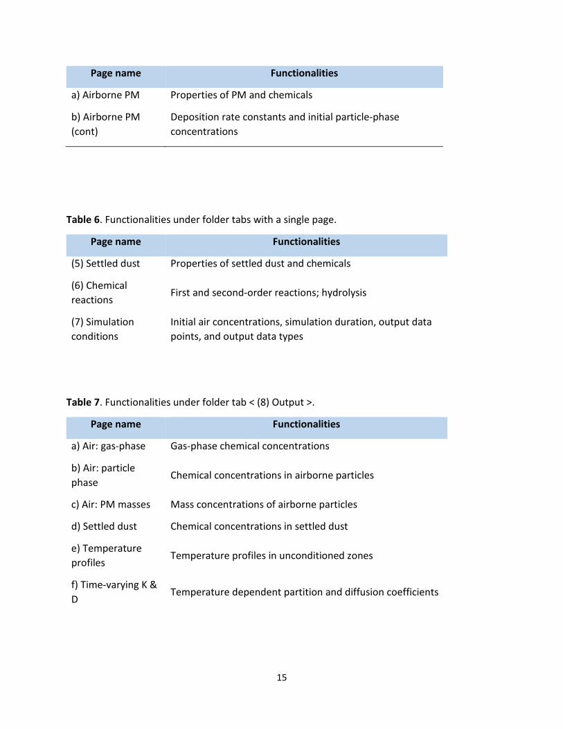
Table 5. Functionalities under folder tab < (4) Airborne PM >.

15

Page name Functionalities

a) Airborne PM Properties of PM and chemicals

b) Airborne PM (cont)

Deposition rate constants and initial particle-phase concentrations

Table 6. Functionalities under folder tabs with a single page.

Page name Functionalities

(5) Settled dust Properties of settled dust and chemicals

(6) Chemical reactions

First and second-order reactions; hydrolysis

(7) Simulation conditions

Initial air concentrations, simulation duration, output data points, and output data types

Table 7. Functionalities under folder tab < (8) Output >.

Page name Functionalities

a) Air: gas-phase Gas-phase chemical concentrations

b) Air: particle phase

Chemical concentrations in airborne particles

c) Air: PM masses Mass concentrations of airborne particles

d) Settled dust Chemical concentrations in settled dust

e) Temperature profiles

Temperature profiles in unconditioned zones

f) Time-varying K & D

Temperature dependent partition and diffusion coefficients

16

3.4 Model files

A model created by the user can be saved to an external file for future retrieval. This feature allows the user to enter a set of parameters (e.g., building configuration and air flow matrix) only once.

The model files use file extension “.IEC’. When you save a file, simply type the file name and there is no need to type the file extension. For example, if you type in “MyModel” and then click <Save>, the model file will be saved as “MyModel.IEC”.

3.5 Simulation modes

Three simulation modes are available: <Run normal>, <Run slow>, and <Run batch>. The first two modes run a single simulation at a time. Most simulations should be done with <Run normal>. The <Run slow> mode is for models with “stiff” differential equations. In other words, if numerical difficulty is encountered with <Run normal>, <Run slow> may resolve the problem. The batch mode allows the user to run multiple models unattended. See Tutorial 5 for details.

3.6 Steps for using IECCU

Making a simulation with IECCU involves five steps:

• Create a model • Compile the model (i.e., error-checking by the program) • Inspect the model (i.e., error-checking by user) • Run the model • Examine the results.

More details are illustrated in Tutorial 1.

17

4. Program specifications

4.1 Building and air exchange

4.1.1 Building configuration

This program provides eight types of building configurations with one to three zones. See Section 6.2 for details.

4.1.2 Air exchange flows

This program allows three types of air exchange flows:

Constant air flows ― a single air flow matrix

Enhanced ventilation in early hours followed by constant flows ― two air flow matrixes

Time-varying air flows ― data is imported from an external file.

4.1.3 Location of HVAC system

The building configuration can be with or without a heating, ventilation and air-conditioning (HVAC) system, which can be located either outside the building or in an unconditioned zone (e.g., garage, crawl space, or attic).

4.1.4 Temperature profiles in unoccupied zones

The temperature profile in an unconditioned zone can be constant, diurnal, seasonal and the combination of the last two. See Section 6.4 for more details.

18

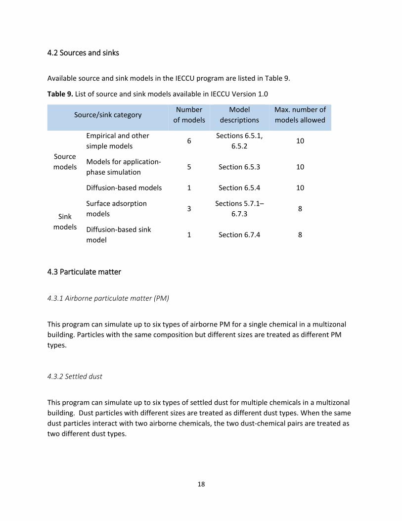
4.2 Sources and sinks

Available source and sink models in the IECCU program are listed in Table 9.

Table 9. List of source and sink models available in IECCU Version 1.0

Source/sink category Number

of models Model

descriptions Max. number of models allowed

Source models

Empirical and other simple models

6 Sections 6.5.1,

6.5.2 10

Models for application-phase simulation

5 Section 6.5.3 10

Diffusion-based models 1 Section 6.5.4 10

Sink models

Surface adsorption models

3 Sections 5.7.1–

6.7.3 8

Diffusion-based sink model

1 Section 6.7.4 8

4.3 Particulate matter

4.3.1 Airborne particulate matter (PM)

This program can simulate up to six types of airborne PM for a single chemical in a multizonal building. Particles with the same composition but different sizes are treated as different PM types.

4.3.2 Settled dust

This program can simulate up to six types of settled dust for multiple chemicals in a multizonal building. Dust particles with different sizes are treated as different dust types. When the same dust particles interact with two airborne chemicals, the two dust-chemical pairs are treated as two different dust types.

19

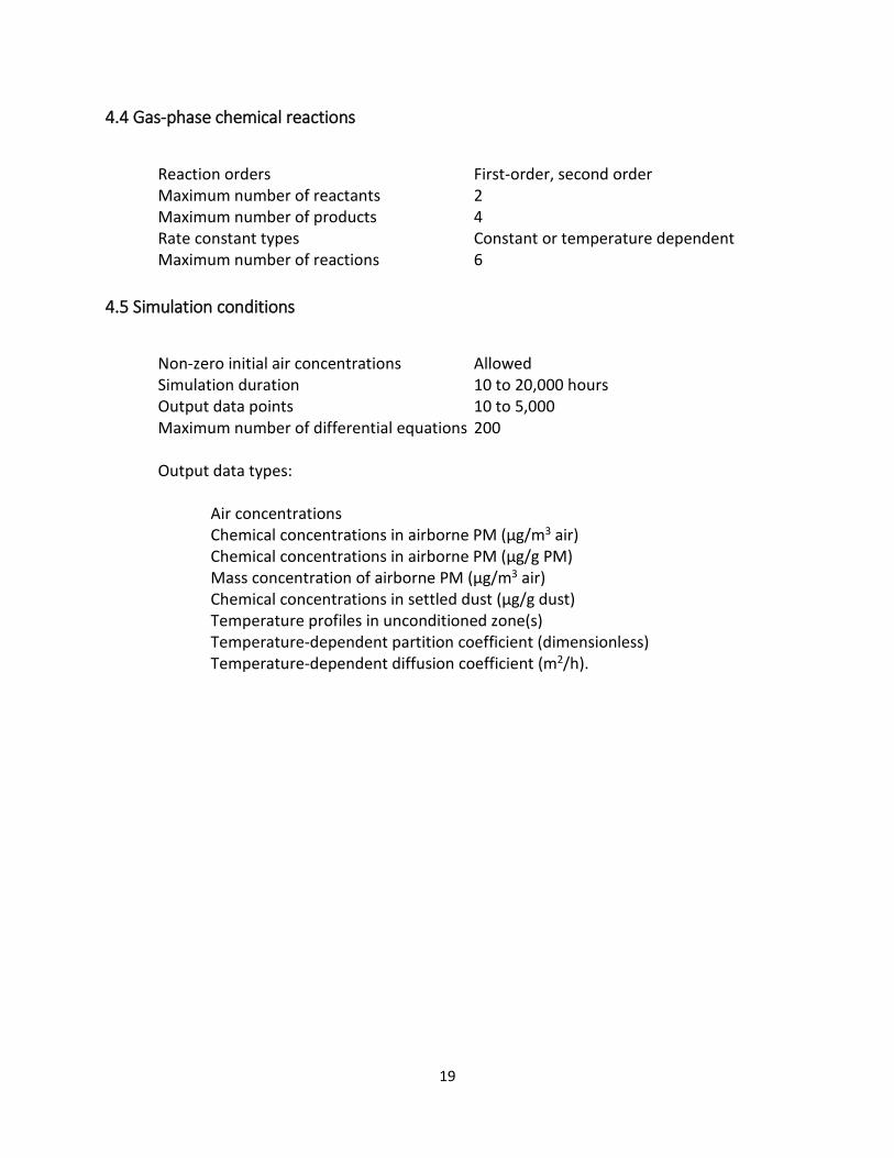
4.4 Gas-phase chemical reactions

Reaction orders First-order, second order Maximum number of reactants 2 Maximum number of products 4 Rate constant types Constant or temperature dependent Maximum number of reactions 6

4.5 Simulation conditions

Non-zero initial air concentrations Allowed Simulation duration 10 to 20,000 hours Output data points 10 to 5,000 Maximum number of differential equations 200 Output data types:

Air concentrations Chemical concentrations in airborne PM (µg/m3 air) Chemical concentrations in airborne PM (µg/g PM) Mass concentration of airborne PM (µg/m3 air) Chemical concentrations in settled dust (µg/g dust) Temperature profiles in unconditioned zone(s) Temperature-dependent partition coefficient (dimensionless) Temperature-dependent diffusion coefficient (m2/h).

20

5. Tutorials

Twelve tutorials are provided in a separate document, entitled Program IECCU 1.0 Tutorials. A summary is shown in Table 10. These tutorials provide examples of exposure scenarios that could be evaluated using IECCU and allow the user to familiarize him/herself with this program and explore its full functionality.

Table 10. List of tutorials.

Tutorial No. Topic

1 Creating a simplest model

2 Using enhanced ventilation

3 TCPP emissions from SPF installed in attic

4 Temperature-dependent TCPP emissions

5 Using the batch mode

6 Gas-phase chemical reactions

7 TCPP interactions with airborne particulate matter (PM)

8 TCPP interactions with settled dust

9 Application-phase simulation

10 Importing indoor-outdoor and zone-to-zone air flow data

11 Importing indoor temperature data

12 Including an HVAC system

21

6. Technical details

6.1 General mass balance equation

The general mass balance equation (Equation 1) for a chemical of interest is used to calculate the time series of indoor concentrations (Bevington et al., 2017). This equation combines all processes governing source emissions, convective transfer by bulk air, sorption and re-remission by indoor sinks, interactions with airborne particles and settled dust and gas-phase chemical reactions.

𝑉𝑉𝑖𝑖𝑑𝑑𝐶𝐶𝑖𝑖𝑑𝑑𝑑𝑑

= ∑ 𝐴𝐴𝑗𝑗𝐸𝐸𝑗𝑗𝑛𝑛1𝑗𝑗=1 − ∑ 𝑄𝑄𝑖𝑖𝑖𝑖

𝑛𝑛2𝑖𝑖=0 𝐶𝐶𝑖𝑖 + ∑ 𝑄𝑄𝑖𝑖𝑖𝑖

𝑛𝑛3𝑖𝑖=0 𝐶𝐶𝑖𝑖 − ∑ 𝑑𝑑𝑚𝑚

𝑛𝑛4𝑚𝑚=1 − ∑ 𝑟𝑟𝑝𝑝

𝑛𝑛5𝑝𝑝=1 ± 𝑉𝑉𝑖𝑖 ∑ 𝑥𝑥𝑞𝑞

𝑛𝑛6𝑞𝑞=1 (1)

where Vi = volume of zone i (m3), Ci = air concentration in zone i (μg/m3), t = time (h), Aj = area of source j in zone i (m2), Ej = emission factor for source j in zone i (μg/m2/h), Qik = air flow from zone i to zone k, i ≠ k (m3/h), Qki = air flow from zone k to zone i, k ≠ i (m3/h), Ck = air concentration in zone k (μg/m3), dm = sorption rate onto interior surface m in zone i (μg/h), rp = rate of sorption by particulate matter p in zone i (μg/h), xq = rate of gas-phase chemical reaction q in zone i, plus sign for products and minus sign for reagents (see notes below for units), Subscripts j, k, l, m, p, and q are summation counters n1 through n6 are item numbers for their respective summations.

When chemical reactions are involved, the mass unit must be in either moles or molecules. For example, term x in Equation 1 should be in either (mol/m3/h) or (molecules/m3/h) in the rate calculation.

22

6.2 Built-in building configurations

This program provides eight built-in building configurations in two categories: (1) All zones are conditioned, and (2) With unconditioned zones, as shown in Table 8. An unconditioned zone is defined as an indoor space where temperature is subject to diurnal, seasonal, or other types of fluctuations. Examples of unconditioned zones in residential buildings include the attic, crawlspace, basement, and garage. If a diffusion source is located in an unconditioned zone, the key source parameters (diffusion and partition coefficients) can change with temperature.

Table 8. IECCU’s built-in building configurations.

Category Conditioned zones Unconditioned zones

All zones are conditioned

One zone None

Two zones None

Three zones (Configuration 1) None

Three zones (Configuration 2) None

With unconditioned zones

Living area Attic

Living area Crawlspace or basement

Living area Attic and crawlspace

Living area Garage

6.3 Indoor-outdoor and zone-to-zone air flows

The indoor-outdoor and zone-to-zone air flows are represented by a (Z+1) × (Z+1) matrix (Q) where Z is the number of air zones. The ambient air is designated zone 0. Element Qij (i ≠ j) is the air flow from zone i to zone j.

In addition to constant air flows, this program has the following features:

• Allowing a period of enhanced ventilation (page < b) Ventilation (1) >) (See Tutorial 2.) • Importing air flow data from CSV files generated by other models such as CONTAM and

COMIS (page < c) Ventilation (2) >). (See Tutorial 10.)

23

6.4 Indoor temperatures

This program provides two ways to represent the temperatures in unconditioned zones:

• User-defined sine functions (page < d) Temperature (1) >) • Imported temperature data table (page < e) Temperature (2) >). (See Tutorial 11).

6.4.1 User-defined temperature functions

Diurnal and seasonal temperature fluctuations are commonly modeled with either sine or cosine functions. In this program, the sine function (Equation 2) is used. An example of simulated temperature profile is shown in Figure 2.

𝑇𝑇 = 𝑇𝑇0 + A sin[𝜔𝜔(𝑡𝑡 − 𝛼𝛼)] (2)

where T = temperature at time t (⁰C), T0 = vertical shift (i.e., average temperature) (⁰C), A = amplitude (⁰C), 2π/ω = period (one day or one year), t = elapsed time, α = horizontal shift.

-20

-10

0

10

20

30

40

50

0 50 100 150 200 250 300 350 400

Tem

pera

ture

(°C)

Elapsed Days

Baseline = 15 °C

August 1 = 40 °C

February 1 = -10 °C

April 2 = 15 °C

24

Figure 2. Simulated annual temperature fluctuation with T0 = 15 ⁰C, A = 25 ⁰C and assuming the peak temperature occurs on August 1. With zero horizontal shift (i.e., α= 0), the elapsed time zero is April 2.

6.4.2 Imported temperature data table

This program allows the user to import zone temperature data generated by other models such as CONTAM and COMIS. It is required that the data table be stored in a comma separated values (CSV) file (See Tutorial 11).

6.5 Source models

6.5.1 Empirical source models

Empirical source models are often used for short-term emissions. This program includes four commonly used empirical models: constant emission source, first-order decay source, dual first-order decay source, and power law (Equations 3 through 6). Brief descriptions on these empirical models can be found in Guo (2002). Model descriptions are also available within the program.

𝑅𝑅 = 𝑐𝑐𝑐𝑐𝑐𝑐𝑐𝑐𝑡𝑡𝑐𝑐𝑡𝑡 (3)

𝑅𝑅 = 𝐴𝐴 𝐸𝐸0 𝑒𝑒−𝑖𝑖 𝑑𝑑 (4a)

𝑅𝑅 = 𝐴𝐴 𝑀𝑀0 𝑘𝑘 𝑒𝑒−𝑖𝑖 𝑑𝑑 (4b)

𝑅𝑅 = 𝐴𝐴 (𝐸𝐸1 𝑒𝑒−𝑖𝑖1 𝑑𝑑 + 𝐸𝐸2 𝑒𝑒−𝑖𝑖2 𝑑𝑑) (5a)

𝑅𝑅 = 𝐴𝐴 (𝑀𝑀1 𝑘𝑘1 𝑒𝑒−𝑖𝑖1 𝑑𝑑 + 𝑀𝑀2 𝑘𝑘2 𝑒𝑒−𝑖𝑖2 𝑑𝑑) (5b)

𝑅𝑅 = 𝐴𝐴 𝑎𝑎𝑑𝑑𝑏𝑏

(6)

where R = emission rate (µg/h), A = source area (m2), E0, E1, E2 = initial emission factor (µg/m2/h), E1 = initial emission factor for rapid emissions (µg/m2/h), E2 = initial emission factor for slow emissions (µg/m2/h),

25

M0 = initial emittable mass of chemical in the source (µg/m2), M1 = initial emittable mass of chemical in the source for rapid emission (µg/m2), M1 = initial emittable mass of chemical in the source for slow emission (µg/m2),

k = first-order decay rate constant (h-1), k1 = first-order decay rate constant for rapid emission (h-1), k2 = first-order decay rate constant for slow emission (h-1),

t = time (h), a, b = empirical constants.

Equations 4a and 4b are equivalent; so are Equations 5a and 5b.

6.5.2 Generic models for chemical emissions from water and aqueous solutions

The rate of chemical emission from contaminated water or aqueous solution can be described by the two-resistance theory with Equation 7 or, equivalently, 8 (Layman et al., 1990):

𝑅𝑅 = 𝐴𝐴 𝐾𝐾𝑂𝑂𝑂𝑂 �𝐶𝐶𝑂𝑂 − 𝐶𝐶𝐻𝐻� (7)

𝑅𝑅 = 𝐴𝐴 𝐾𝐾𝑂𝑂𝑂𝑂 (𝐶𝐶𝑂𝑂𝐻𝐻 − 𝐶𝐶) (8)

where R = emission rate (µg/h) A = exposed area of liquid (m2) KOL = overall liquid-phase mass transfer coefficient (m/h) KOG = overall gas-phase mass transfer coefficient (m/h) CL = chemical concentration in water (µg/m3) C = chemical concentration in air (µg/m3) H = dimensionless Henry’s law constant and H = CG / CL at equilibrium.

6.5.3 Application-phase models

Most source emission models treat the source area as a constant. For sources such as painted walls and application of spray polyurethane foam insulation, it takes a substantial amount of time for the source area to increase from zero to the final area. Thus, to predict the short-term emissions from such sources, the source area should be treated as a variable. The algorithm for

26

application-phase simulation is described in IAQX (EPA, 2000). Four empirical models can be used for the emissions from an incremental piece of source:

• Rapid evaporation (i.e., instant emissions) • First-order decay (Equation 4b) • Dual first-order decay source (Equation 5b) • Power law model (Equation 6).

Tutorial 9 shows an example of an application-phase simulation.

6.5.4 Diffusion-based models

The emission of a chemical from a solid material and the diffusion of the chemical inside the solid material are represented by the modified state-space (MSS) method, which divides the solid phase into a finite number of slices or hollow spheres (Figure 3). More details about the method development and validation can be found in Guo (2013). This method is more flexible than other diffusion models because it permits:

• Multiple air zones • Multiple sources and sinks • Non-uniform initial concentrations in the source or sink • Non-zero initial air concentrations.

Figure 3. Representation of diffusion sources by the MSS method (not to scale).

27

Mass transfer between the top slice and room air:

−= a

ma

mama C

KCHAR 1 (9)

ammaa hhKH111

+= (10)

1

2LDh m

m ∆= (11)

where Rma = rate of mass transfer from the top (exposed) slice to air (μg/h) A = exposed area of the source or sink (m2) Ha = overall gas-phase mass transfer coefficient (m/h) from Equation 10 (m/h) Cm1 = SVOC concentration in the top (exposed) slice of the source or sink (μg/m3) Kma = solid-air partition coefficient (dimensionless) Ca = SVOC concentration in room air (μg/m3). ha = gas-phase mass transfer coefficient (m/h)

hm = solid-phase mass transfer coefficient, from Equation 11 (m/h) Dm = solid-phase diffusion coefficient (m2/h) ∆L1 = thickness of the top (exposed) slice (m). Note that the solid-phase mass transfer coefficient is not only a function of diffusion coefficient but also a function of the thickness of the slice. Mass transfer between two adjacent slices of the same material:

( )mjmimij CChAR −= (12)

ji

mm LL

Dh∆+∆

=2

(13)

where Rij = rate of mass transfer from slice i to slice j (μg/h)

28

hm = solid-phase mass transfer coefficient (m/h) Dm = solid-phase diffusion coefficient (m2/h) ∆Li, ∆Lj = thicknesses of slices i and j (m)

(∆Li+ ∆Lj)/2 = travel distance for inter-slice diffusion (m) Cmi = concentration in slice i (μg/m3) Cmj = concentration in slice j (μg/m3). Thicknesses and number of slices The thickness of the exposed slice is set to 1 µm. The thicknesses of the interior slices are determined by their depths: the ratio of the thicknesses of two adjacent slices is 1:2 (See Figure 3). The number of the MSS slices is determined by the thickness of the source. If the source is 1 cm or less, ten slices will be used; otherwise, 15 slices.

6.6 Temperature-dependent emission parameters

The temperature dependence of partition and diffusion coefficients are estimated using existing empirical models. Currently the program provides two methods for estimating partition coefficients and three methods for solid-phase diffusion coefficient. Additional methods can be added later. See Tutorial 4 for an example of modeling temperature-dependent emissions.

6.6.1 Partition coefficient

Method 1 (Zhang et al., 2007):

𝐾𝐾 = 𝐴𝐴1 𝑇𝑇0.5 𝑒𝑒𝐴𝐴2/ 𝑇𝑇 (14)

where K = solid-air partition coefficient at temperature T (dimensionless), T = absolute temperature (K), A1, A2 = empirical constants for a given material/chemical pair.

29

Method 2 (Tian et al., 2017):

𝑙𝑙𝑐𝑐 𝐾𝐾2𝐾𝐾1

= 𝑎𝑎 𝛥𝛥𝐻𝐻𝑣𝑣𝑅𝑅

� 1𝑇𝑇2− 1

𝑇𝑇1� (15)

where K1, K2 = partition coefficient at temperatures T1 and T2 (dimensionless), ΔHv = vaporization enthalpy (J), T1, T2 = absolute temperature corresponding to K1 and K2 (K), R = gas constant (J/mol/K)

a = absolute value of the slope for the ln(K)-ln(P) relationship, where P is the vapor pressure.

6.6.2 Solid-phase diffusion coefficient

Method 1 (Begley, 2005):

ln𝐷𝐷 = 𝐴𝐴𝑝𝑝 − 0.101 𝑚𝑚 − 10450 / 𝑇𝑇 (16)

where D = solid-phase diffusion coefficient at temperature T (m2/s), Ap = material-specific constant

m = molecular weight of chemical (g/mol), T = absolute temperature (K).

Method 2 (Dole et al., 2006):

ln𝐷𝐷 = 𝐴𝐴𝑝𝑝 − 0.101 𝑚𝑚 − 10450 / 𝑇𝑇 (17)

where D = solid-phase diffusion coefficient at temperature T (m2/s), Ap = material specific coefficient m = molecular weight of chemical (g/mol), T = absolute temperature (K).

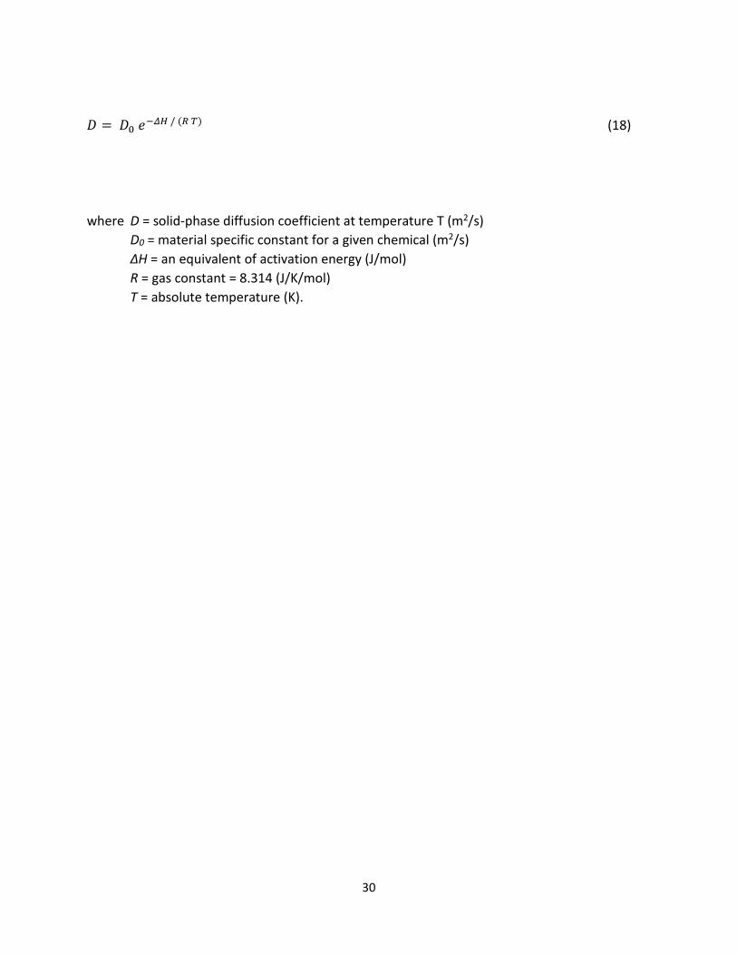
Method 3 (Tian et al., 2017):

30

𝐷𝐷 = 𝐷𝐷0 𝑒𝑒−𝛥𝛥𝐻𝐻 / (𝑅𝑅 𝑇𝑇) (18)

where D = solid-phase diffusion coefficient at temperature T (m2/s) D0 = material specific constant for a given chemical (m2/s)

ΔH = an equivalent of activation energy (J/mol) R = gas constant = 8.314 (J/K/mol) T = absolute temperature (K).

31

6.7 Sink models

Interior surfaces can act as a reservoir, or sink, of airborne pollutants. This sink effect is especially important for SVOCs. Four sink models are implemented in this program:

• First-order reversible Langmuir sink • Freundlich reversible sink • First-order irreversible sink • Molecular diffusion based sink.

6.7.1 First-order reversible Langmuir sink

The adsorption and desorption rates for the dynamic Langmuir sink are given by Equations 19 and 20 (Tichenor et al., 1991): 𝑅𝑅𝑎𝑎 = 𝐴𝐴 𝑘𝑘𝑎𝑎 𝐶𝐶𝑎𝑎 (19)

𝑅𝑅𝑑𝑑 = 𝐴𝐴 𝑘𝑘𝑑𝑑 𝐶𝐶𝑠𝑠 (20)

where Ra = adsorption rate (μg/h) Rd = desorption rate (μg/h) A = area of sink surface (m2) ka = adsorption rate constant (m/h) kd = desorption rate constant (h-1) Ca = concentration in air (μg/m3) Cs = concentration on sink surface (μg/m2).

6.7.2 Freundlich reversible sink The adsorption and desorption rates for the dynamic Freundlich sink are given by Equation 21 and 22 (Van Loyd et al., 1997): 𝑅𝑅𝑎𝑎 = 𝐴𝐴 𝑓𝑓𝑎𝑎 𝐶𝐶𝑎𝑎𝛼𝛼 (21)

𝑅𝑅𝑑𝑑 = 𝐴𝐴 𝑓𝑓𝑑𝑑 𝐶𝐶𝑎𝑎𝛽𝛽 (22)

where Ra = adsorption rate (μg/h) Rd = desorption rate (μg/h) A = area of sink surface (m2) fa = nonlinear adsorption rate constant (μg1-α m3α-2 h-1)

32

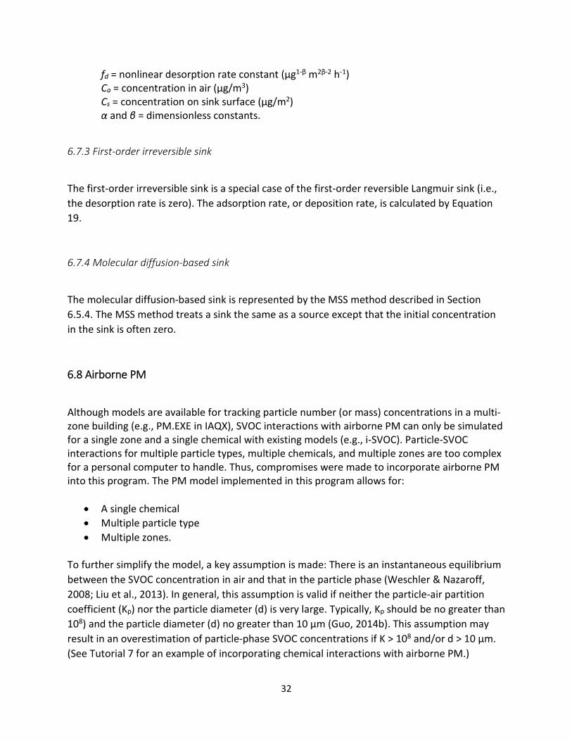
fd = nonlinear desorption rate constant (μg1-β m2β-2 h-1) Ca = concentration in air (μg/m3) Cs = concentration on sink surface (μg/m2) α and β = dimensionless constants.

6.7.3 First-order irreversible sink

The first-order irreversible sink is a special case of the first-order reversible Langmuir sink (i.e., the desorption rate is zero). The adsorption rate, or deposition rate, is calculated by Equation 19.

6.7.4 Molecular diffusion-based sink

The molecular diffusion-based sink is represented by the MSS method described in Section 6.5.4. The MSS method treats a sink the same as a source except that the initial concentration in the sink is often zero.

6.8 Airborne PM

Although models are available for tracking particle number (or mass) concentrations in a multi-zone building (e.g., PM.EXE in IAQX), SVOC interactions with airborne PM can only be simulated for a single zone and a single chemical with existing models (e.g., i-SVOC). Particle-SVOC interactions for multiple particle types, multiple chemicals, and multiple zones are too complex for a personal computer to handle. Thus, compromises were made to incorporate airborne PM into this program. The PM model implemented in this program allows for:

• A single chemical • Multiple particle type • Multiple zones.

To further simplify the model, a key assumption is made: There is an instantaneous equilibrium between the SVOC concentration in air and that in the particle phase (Weschler & Nazaroff, 2008; Liu et al., 2013). In general, this assumption is valid if neither the particle-air partition coefficient (Kp) nor the particle diameter (d) is very large. Typically, Kp should be no greater than 108) and the particle diameter (d) no greater than 10 µm (Guo, 2014b). This assumption may result in an overestimation of particle-phase SVOC concentrations if K > 108 and/or d > 10 µm. (See Tutorial 7 for an example of incorporating chemical interactions with airborne PM.)

33

6.9 Settled dust The interactions of airborne chemicals with settled dust are calculated by the modified state-space (MSS) method (Guo, 2013), which divides a spherical dust particle into a finite number of concentric hollow spheres (Figure 4). More details about the method development and validation can be found in Guo (2014a).

Figure 4. Representation of dust particles by the MSS method. The exposed hollow sphere is 0.1 µm thick. The thicknesses of interior hollow spheres depend on their depths. For example, (r3 - r2) = 2 × (r2 - r1) 6.9.1 Mass transfer between room air and the exposed hollow sphere

−=

ma

paaap K

CCHAR 1 (23)

appaa hhKH111

+= (24)

)( 0 td

pp rr

Dh

−= (25)

34

where Rap = rate of mass transfer from room air to airborne particles (μg/h) A = surface area of the particle (m2) Ha = overall gas-phase mass transfer coefficient, from Equation 18 (m/h) Cp1 = concentration in the exposed hollow sphere (μg/m3) Kpa = particle-air partition coefficient (dimensionless) Ca = concentration in room air (μg/m3). hp = particle-phase mass transfer coefficient, from Equation 19 (m/h) Dp = particle-phase diffusion coefficient (m2/h) r0 = radius of the particle (m)

rtd = radius that divides the top hollow sphere into two parts with equal volumes (Equation 26).

)(34)(

34 3

1333

0 rrrr tdtd −=− ππ (26)

where r0 = outside radius of the top hollow sphere (m) r1 = inside radius of the top hollow sphere (m).

6.9.2 Mass transfer within the particle

The rate of mass transfer between two adjacent hollow spheres, i and j, is determined by Equation 27:

( )pjpipiij CChAR −= (27)

24 ii rA π= (28)

tdjtdi

pp rr

Dh

−=

(29)

where Rij = rate of mass transfer from hollow sphere i to hollow sphere j (μg/h) Ai = contact area for hollow spheres i and j, from Equation 28 (m2)

hp = particle-phase mass transfer coefficient between hollow spheres i and j, from Equation 29 (m/h) ri = inside radius of hollow sphere i (i.e., the outer hollow sphere) (m) rtdi = radius for travel distance in hollow sphere i, from Equation 26 (m) rtdj = radius for travel distance in hollow sphere j, from Equation 26 (m) (rtdi – rtdj) = travel distance between two adjacent hollow spheres i and j (m).

35

6.9.3 Thicknesses and number of concentric hollow spheres The thickness of the exposed hollow sphere is set to 0.1 µm. The thicknesses of the interior slices are determined by their depths: ratio of the thicknesses of two adjacent slices it 1:2 (See Figure 4). The number of the hollow spheres is determined by the diameter of the dust particles. If the diameter is 10 µm or less, three hollow spheres will be used; otherwise, five hollow spheres.

6.10 Gas-phase chemical reactions

This program allows the user to define a limited number of gas-phase chemical reactions. Because chemical reactions take place on a molecule-to-molecule (i.e., mole-to-mole) basis, unit conversion is necessary to incorporate chemical reactions. This conversion is performed by the program and the user needs only to provide the molecular weight of the chemical species involved. See Tutorial 6 for an example of incorporating chemical reactions in a model.

6.10.1 First-order reaction

The generic form of first-order reactions is shown in Equation 30:

𝑅𝑅1 = 𝑦𝑦1 𝑃𝑃1 + 𝑦𝑦2 𝑃𝑃2 + ⋯ (30)

where R1 = reactant, P1, P2, … = products, y1, y2, … = product yields.

The rate is calculated according to Equations 31 and 32:

𝑑𝑑[𝑅𝑅1]𝑑𝑑𝑑𝑑

= −𝑘𝑘1 [𝑅𝑅1] (31)

𝑑𝑑[𝑃𝑃1]𝑑𝑑𝑑𝑑

= 𝑘𝑘1 𝑦𝑦1 [𝑅𝑅1] (32)

36

where [R] = gas-phase concentration of the reactant (molecules/cm3) t = time (s)

[P1] = gas-phase concentration of product 1 (molecules/cm3) k1 = first-order reaction constant (s-1).

6.10.2 Second-order reaction

A second-order reaction can be in the form of either Equation 33 or 34:

𝑅𝑅1 + 𝑅𝑅2 = 𝑦𝑦1 𝑃𝑃1 + 𝑦𝑦2 𝑃𝑃2 + ⋯ (33)

2 𝑅𝑅1 = 𝑦𝑦1 𝑃𝑃1 + 𝑦𝑦2 𝑃𝑃2 + ⋯ (34)

where R1, R2 = reactants P1, P2, … = products y1, y2, … = product yields.

The reaction rate is calculated from Equations 35 and 36:

𝑑𝑑[𝑅𝑅1]𝑑𝑑𝑑𝑑

= 𝑑𝑑[𝑅𝑅2]𝑑𝑑𝑑𝑑

= −𝑘𝑘2 [𝑅𝑅1] [𝑅𝑅2] (35)

𝑑𝑑[𝑃𝑃1]𝑑𝑑𝑑𝑑

= 𝑘𝑘2 𝑦𝑦1 [𝑅𝑅1] [𝑅𝑅2] (36)

where k2 = second-order reaction constant (molecule-1 m3 s).

6.10.3 Temperature-dependence of reaction rate constants

This program uses a simplified version of the Arrhenius equation (Equation 37) to calculate temperature-dependent rate constants.

𝑘𝑘(𝑇𝑇) = 𝐴𝐴 𝑒𝑒−𝐸𝐸𝑎𝑎/𝑇𝑇 (37)

37

where k(T) = rate constant at temperature T, A = constant specific to a chemical reaction, Ea = a lumped parameter (i.e., activation energy divided by gas constant), T = temperature (K).

38

References

Begley, T., Castle, L., Feigenbaum, A., Franz, R., Hinrichs, K., Lickly, T., Mercea, P., Milana, M., O'Brien, A., Rebre, S., Rijk, R., and Piringer, O. (2005). Evaluation of migration models that might be used in support of regulations for food-contact plastics. Food Additives & Contaminants, 22(1):73-90.

Bevington, C., Guo, Z., Hong, T., Hubbard, H., Wong, E., Sleasman, K., and Hetfield, H. (2017). A modeling approach to quantify exposures from emissions of spray polyurethane foam insulation in indoor environments. In: ASTM STP 1589― Developing Consensus Standards for Measuring Chemical Emissions from Spray Polyurethane Foam (SPF) Insulation, pp 199-227.

Dole, P., Feigenbaum, A.E., De La Cruz, C., Pastorelli, S., Paseiro, P., Hankemeier, T., Voulzatis, Y., Aucejo, S., Saillard, P., Papaspyrides, C. (2006). Typical diffusion behaviour in packaging polymers – application to functional barriers. Food Additives & Contaminants, 23(2): 202-211.

EPA (2000). Simulation Tool Kit for Indoor Air Quality and Inhalation Exposure (IAQX) Version 1.0 User’s Guide, U.S. Environmental Protection Agency, National Risk Management Research Laboratory, Research Triangle Park, NC, Report No. EPA-600/R-00-094, 76 pp. https://www.epa.gov/air-research/simulation-tool-kit-indoor-air-quality-and-inhalation-exposure-iaqx

EPA (2013). Simulation program i-SVOC user’s guide, U.S. EPA Report EPA/600/R-13/212. http://nepis.epa.gov/Exe/ZyPURL.cgi?Dockey=P100HYEF.txt

Guo, Z. (2002). Review of indoor emission source models – Part 1. Overview. Environmental Pollution, 120: 533-549.

Guo, Z. (2013). A framework for modeling non-steady state concentrations of semivolatile organic compounds indoors ― I. Emissions from diffusional sources and sorption by interior surfaces. Indoor and Built Environment, 22:685–700.

Guo, Z. (2014a). A framework for modeling non-steady state concentrations of semivolatile organic compounds indoors ― II. Interactions with particulate matter. Indoor and Built Environment, 23:26–43.

Guo, Z. (2014b). Improve our understanding of semivolatile organic compounds in buildings. Indoor and Built Environment, 23:769-773.

Huang, L., Fantke, P., Ernstoff, A., & Jolliet, O. A Quantitative Property-Property Relationship for the Internal Diffusion Coefficients of Organic Compounds in Solid Materials. Indoor Air.

39

Lyman, W. L., Reehl, W. F., Rosenblatt, D. H. (1990). Handbook of chemical property estimation methods: environmental behavior of organic compounds. American Chemical Society, Washington, DC.

Liu, C., Shi, S., Weschler, C., Zhao, B., and Zhang, Y. (2013). Analysis of the dynamic interaction between SVOCs and airborne particles. Aerosol Science & Technology, 47: 125-136.

Tian, S., Sebroski, J., and Ecoff, S. (2017). Predicting TCPP Emissions and Airborne Concentrations from Spray Polyurethane Foam Using USEPA i-SVOC software: Parameter Estimation and Result Interpretation. In: ASTM STP 1589 ― Developing Consensus Standards for Measuring Chemical Emissions from Spray Polyurethane Foam (SPF) Insulation, pp 167-198.

Tichenor, B.A., Guo, Z., Dunn, J.E., Sparks, L.E. and Mason, M.A. (1999). The interaction of vapor phase organic compounds with indoor sinks, Indoor Air, 1:23-35. Van Loy, M.D., Lee, V.C., Gundel, L.A., Daisey, J. M., Sextro, R.G. and Nazaroff, W.W. (1997). Dynamic behavior of semivolatile organic compounds in indoor air. 1. Nicotine in a stainless steel chamber, Environmental Science & Technology, 31:2554-2561. Weschler, C.J. and Nazaroff, W.W. (2008). Semivolatile organic compounds in indoor environments, Atmospheric Environment, 42:9018–9040. Xiong, J., Wei, W., Huang, S., Zhang, Y. (2013). Association between the emission rate and temperature for chemical pollutants in building materials: General correlation and understanding. Environmental Science & Technology, 47(15):8540-8547.

Zhang, Y., Xiaoxi Luo, X., Wang, X., Qian, K., and Zhao, R. (2007). Influence of temperature on formaldehyde emission parameters of dry building materials. Atmospheric Environment, 41(15): 3203–3216.

40

IECCU 1.0 Tutorials Appendix

41

Contents

Introduction ................................................................................................................................................ 45

Tutorial 1: Creating a simplest model ......................................................................................................... 46

1.1 Objective ........................................................................................................................................... 46

1.2 Case description ................................................................................................................................ 46

1.3 Create the model .............................................................................................................................. 47

1.3.1 Define building configuration .................................................................................................... 47

1.3.2 Define ventilation flow rate ....................................................................................................... 48

1.3.3 Define the source ....................................................................................................................... 49

1.3.4 Define simulation conditions ..................................................................................................... 51

1.4 Compile the model ............................................................................................................................ 53

1.5. Inspect the model ............................................................................................................................ 53

1.6 Run the model ................................................................................................................................... 54

1.7 Examine the results ........................................................................................................................... 54

Tutorial 2: Using enhanced ventilation ....................................................................................................... 56

2.1 Objective ........................................................................................................................................... 56

2.2 Case description ................................................................................................................................ 56

2.3 Create the model .............................................................................................................................. 56

2.4 Save, compile and run the model ..................................................................................................... 57

Tutorial 3: TCPP emissions from SPF installed in attic ................................................................................ 59

3.1 Objective ........................................................................................................................................... 59

3.2 Case description ................................................................................................................................ 59

3.3. Create the model ............................................................................................................................. 61

3.3.1 Select building configuration ..................................................................................................... 61

3.3.2 Define air flow matrix ................................................................................................................ 62

3.3.3 Define the source ....................................................................................................................... 63

3.3.4 Define the sink ........................................................................................................................... 64

3.3.5 Define simulation conditions ..................................................................................................... 66

3.4 Save, compile, inspect, and run the model ....................................................................................... 67

Tutorial 4: Simulating temperature-dependent TCPP emissions ............................................................... 69

42

4.1 Objective ........................................................................................................................................... 69

4.2 Case description ................................................................................................................................ 69

4.3 Create the model .............................................................................................................................. 70

4.3.1 Define temperature profile in attic ............................................................................................ 70

4.3.2 Modify the SPF source ............................................................................................................... 73

4.3.3 Define temperature-dependent functions for partition coefficient .......................................... 75

4.3.4 Define temperature-dependent functions for diffusion coefficient .......................................... 78

4.3.5 Select output data types ............................................................................................................ 79

4.4 Save, compile, inspect and run the model ........................................................................................ 79

Tutorial 5: Using the batch mode ............................................................................................................... 82

5.1 Objective ........................................................................................................................................... 82

5.2 General steps .................................................................................................................................... 82

5.3 Case description ................................................................................................................................ 82

5.4 Run batch .......................................................................................................................................... 82

5.4.1 Create an empty folder .............................................................................................................. 82

5.4.2 Save or copy model files to that folder ...................................................................................... 82

5.4.3 Run batch simulations ................................................................................................................ 83

5.4.4 Retrieve simulation results ........................................................................................................ 87

Tutorial 6: Gas-phase chemical reactions ................................................................................................... 88

6.1 Objective ........................................................................................................................................... 88

6.2 Case description ................................................................................................................................ 88

6.3 Create the model .............................................................................................................................. 89

6.3.1 Define building and ventilation .................................................................................................. 89

6.3.2 Define the first-order decay source ........................................................................................... 89

6.3.3 Define the chemical reaction ..................................................................................................... 90

6.3.4 Define simulation conditions ..................................................................................................... 92

6.4 Save, compile, inspect and run the model ........................................................................................ 92

Tutorial 7: TCPP interactions with airborne particulate matter (PM) ........................................................ 94

7.1 Objective ........................................................................................................................................... 94

7.2 Case description ................................................................................................................................ 94

7.3. Create the model ............................................................................................................................. 94

7.3.1 Open model MyTCPP-1.IEC ........................................................................................................ 94

7.3.2 Define airborne PM .................................................................................................................... 95

43

7.3.3 Define deposition rate constants and initial PM mass concentrations ..................................... 96

7.3.4 Select output data types ............................................................................................................ 97

7.4 Save, compile, inspect, and run the model ....................................................................................... 99

Tutorial 8: TCPP interactions with settled dust ........................................................................................ 100

8.1 Objective ......................................................................................................................................... 100

8.2 Case description .............................................................................................................................. 100

8.3 Create the model ............................................................................................................................ 100

8.3.1 Load model MyTCPP-PM.IEC ................................................................................................... 100

8.3.2 Define settled dust ................................................................................................................... 100

8.3.3 Define simulation conditions ................................................................................................... 104

8.4 Save, compile, inspect and run the model ...................................................................................... 104

Tutorial 9: Application-phase simulation .................................................................................................. 106

9.1 Objective ......................................................................................................................................... 106

9.2 Case description .............................................................................................................................. 106

9.3 Create the model ............................................................................................................................ 107

9.3.1 Define building configuration .................................................................................................. 107

9.3.2 Define air flow matrices for base and enhanced ventilation ................................................... 107

9.3.3 Define application-phase model .............................................................................................. 108

9.3.4 Define simulation conditions ................................................................................................... 109

9.4 Save, compile, inspect and run the model ...................................................................................... 109

Tutorial 10: Importing indoor-outdoor and zone-to-zone air flow data .................................................. 111

10.1 Objective ....................................................................................................................................... 111

10.2 Case description ............................................................................................................................ 111

10.3 Create the model .......................................................................................................................... 111

10.4 Save, compile, inspect and run the model .................................................................................... 112

Tutorial 11: Importing indoor temperature data ...................................................................................... 114

11.1 Objective ....................................................................................................................................... 114

11.2 Case description ............................................................................................................................ 114

11.3 Create the model .......................................................................................................................... 115

11.4 Save, compile, inspect and run the model .................................................................................... 115

Tutorial 12: Including an HVAC system ..................................................................................................... 117

12.1 Objective ....................................................................................................................................... 117

12.2 Case description ............................................................................................................................ 117

44

12.3 Create the model .......................................................................................................................... 118

12.4 Compile and run the model .......................................................................................................... 122

References ................................................................................................................................................ 124

45

Introduction

This is an appendix of the IECCU User’s Guide containing several tutorials. IECCU is a simulation program for estimating chemical emissions from sources and related changes to Indoor Environmental Concentrations in Buildings with Conditioned and Unconditioned Zones. As such, IECCU is an indoor exposure model. A model simulation is one run of the model and involves creating, compiling, inspecting, and running the model. Users are encouraged to examine their results in comparison to other modeled estimates or indoor monitoring data for a similar exposure scenario, if available.

This document contains 11 tutorials aimed to familiarize the users with most features of this program. Through this practice, the users are expected to design their own scenarios for use with IECCU. To assist this process, the model files for the tutorials are also available from the Secure File Sharing Site where users downloaded the set-up file.

The scenarios and parameters used in these tutorials are intended to cover most of the features of this program. Some of them are real and some are hypothetical, and none are intended to represent specific brands of commercial products. Users are encouraged to use this program to consider their own applications and scenarios.

CAUTION: To demonstrate this program’s capability to simulate sources in unconditioned zones, spray polyurethane foam (SPF) applications were used in several tutorials. Due to the lack of experimental data, most parameters for SPF were obtained either from limited data (such as initial chemical concentration in SPF) or from existing empirical or quantitative structure-activity relationship (QSAR) models (such as the partition coefficient) or based on educated guesses (such as the solid-phase diffusion coefficient) and, thus, may contain large errors.

Disclaimer: The computer software described in this document was developed by the U.S. EPA for its own use and for specific applications. The Agency makes no warranties, either expressed or implied, regarding this computer software package, its merchantability, or its fitness for any particular purpose, and accepts no responsibility for its use. Mention of trade names and commercial products does not constitute endorsement or recommendation for use. The views expressed in this document do not necessarily represent the views or policies of the Agency.

46

Tutorial 1: Creating a simplest model

1.1 Objective

To demonstrate the general steps for using IECCU by creating and running a simplest model. Description of the user interface is given in Section 3 in the Tester’s Guide.

1.2 Case description

Doing a simulation with IECCU involves five steps:

• Create the model, • Compile the model (i.e., error-checking by the program), • Inspect the model (i.e., error-checking by user), • Run the model, • Examine the results.

The first model we will create is for a constant source in a single zone with parameters listed in Table 1.1.

Table 1.1. Parameters for the simplest IECCU model.

Parameter name Value Zone name Bedroom1 Room volume 30 m3

Ventilation flow rate 30 m3/h Chemical name HCHO Constant emission rate 100 µg/h

This simple model will need four input pages:

• Page < a) Air zones > under folder < (1) Building & environment >, • Page < b) Ventilation (1) > under folder < (1) Building & environment >, • Page < a) Empirical models > under folder < (2) Sources >, • Folder/page < (7) Simulation conditions >.

47

1.3 Create the model

Launch IECCU; click the button with a right arrow to proceed (Figure 1.1).

Figure 1.1. IECCU front page.

1.3.1 Define building configuration

The main window is shown in Figure 1.2. The notepad on the left provides a space for the user to make notes, such as a verbal description of the model. Try to type a few words in the box.

The default building configuration is a single unconditioned zone. For this tutorial, there is no need to make any changes. If you want to change the building configuration, click the button < Select building configuration >, which will be described in Section 3.3.1.

Enter “Bedroom1” for zone name and 30 for zone volume. Now you are done with the < a) Air zones > page (see Figure 1.2).

48

Figure 1.2. IECCU main window, showing completed page < a) Air zones > under folder tab < (1) Building & environment >.

1.3.2 Define ventilation flow rate

To enter ventilation data, click the < Ventilation (1) > page tab.

Click the < Visualize > button to view a graphic representation of the air flows.

Enter 30 in the blank cell in Table 1 on top-left corner (the on-screen table is titled “Normal air exchange flow rates (m3/h)”). The completed page is shown in Figure 1.3.

Note that the column for “To zone 0” in the air exchange flow table is not editable because those cells do not require any input from the user.

49

Figure 1.3. Completed page < b) Ventilation (1) > under folder tab < (1) Building & environment>.

1.3.3 Define the source

Click the < (2) Sources > folder tab. There are four pages under this folder. In this tutorial we will use the < a) Empirical models > page.

Click the < Add > button to bring up the input form for empirical source models.

At the top-left corner, click the box for “Empirical source models” (Figure 1.4).

Select “(11) Constant source” from the pull-down menu. Note that the form changed to Figure 1.5.

Enter “HCHO” for the chemical name, then click the pull-down menu for source location and then select “Bedroom1”, and enter 100 for R0 (See Figure 1.5).

Note that chemical names are not case-sensitive. For example, “HCHO”, “hcho” and “Hcho” are the same.

50

Figure 1.4. User input page for empirical source models.

Figure 1.5. Completed user input window for empirical source model 11.

51

Click < OK > to accept the input parameters. Note that if your input contains any errors, an error message will pop up. Correct the error and then click < OK >. The completed page < a) Empirical models > is shown in Figure 1.6.

Figure 1.6. Completed page < a) Empirical models > under folder tab < (2) Sources >.

Note that you can make changes to the items you entered in Figure 1.6. Simply click a cell in the column that you want to make changes and then click the < Edit > button.

1.3.4 Define simulation conditions

Click the < (7) Simulation conditions > folder tab. The table on the left is for initial air concentrations. The default value is zero. In this model, we will use the default value.

From the top right side of the window, use the pull-down list to select 20 hours for simulation duration.

Click the < Select > button to select output data types. Select “1) Air concentrations” from the left panel; click < Select > and then click < OK >. See Figure 1.7.

52

Figure 1.7. Form for selecting output data types

The completed < (7) Simulation conditions > page is shown in Figure 1.8.

Figure 1.8. Completed page < (7) Simulation conditions >.

53

Now, you have finished creating your first model. Save this model using the file name “MyModel-1.IEC” by clicking the < Save > speed button (The third from left). You will need this file later.

1.4 Compile the model

Click the < Compile > speed button to allow the program to check for potential errors in your model. If an error message pops up, correct the error and then try again.

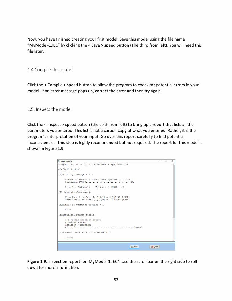
1.5. Inspect the model

Click the < Inspect > speed button (the sixth from left) to bring up a report that lists all the parameters you entered. This list is not a carbon copy of what you entered. Rather, it is the program’s interpretation of your input. Go over this report carefully to find potential inconsistencies. This step is highly recommended but not required. The report for this model is shown in Figure 1.9.

Figure 1.9. Inspection report for ‘MyModel-1.IEC”. Use the scroll bar on the right side to roll down for more information.

54

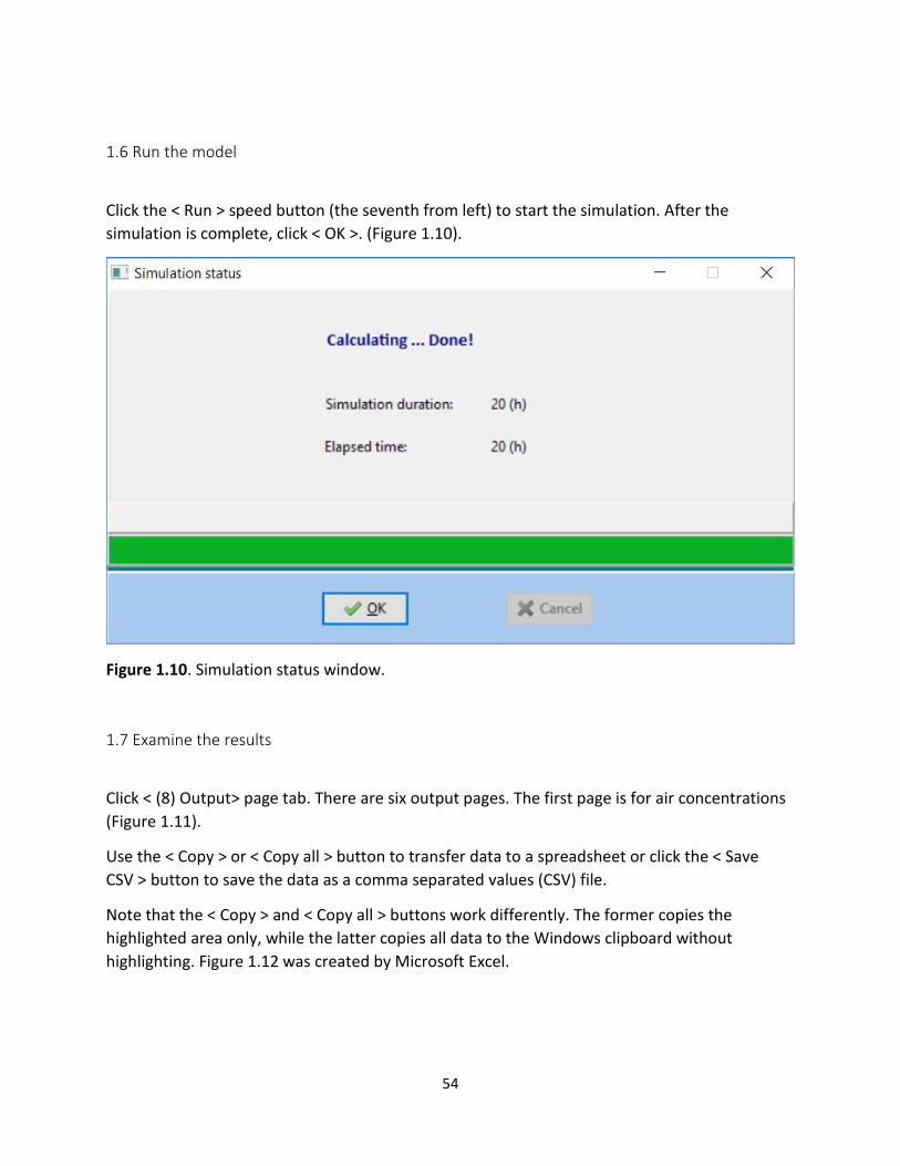
1.6 Run the model

Click the < Run > speed button (the seventh from left) to start the simulation. After the simulation is complete, click < OK >. (Figure 1.10).

Figure 1.10. Simulation status window.

1.7 Examine the results

Click < (8) Output> page tab. There are six output pages. The first page is for air concentrations (Figure 1.11).

Use the < Copy > or < Copy all > button to transfer data to a spreadsheet or click the < Save CSV > button to save the data as a comma separated values (CSV) file.

Note that the < Copy > and < Copy all > buttons work differently. The former copies the highlighted area only, while the latter copies all data to the Windows clipboard without highlighting. Figure 1.12 was created by Microsoft Excel.

55

Figure 1.11. The output page for air concentrations.

Figure 1.12. Simulation results of MyModel-1.IEC. This plot was made with Microsoft Excel.

0

1

2

3

4

0 5 10 15 20

Conc

entr

atio

n (µ

g/m

3 )

Elapsed Time (h)

56

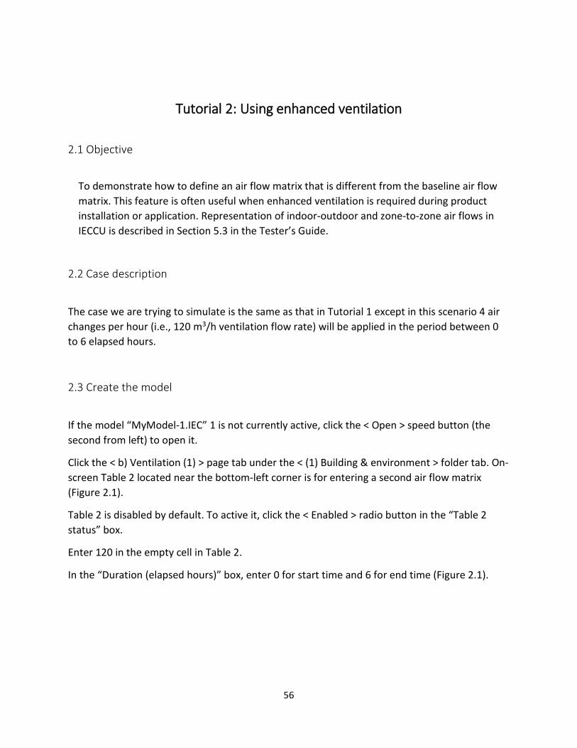
Tutorial 2: Using enhanced ventilation

2.1 Objective

To demonstrate how to define an air flow matrix that is different from the baseline air flow matrix. This feature is often useful when enhanced ventilation is required during product installation or application. Representation of indoor-outdoor and zone-to-zone air flows in IECCU is described in Section 5.3 in the Tester’s Guide.

2.2 Case description

The case we are trying to simulate is the same as that in Tutorial 1 except in this scenario 4 air changes per hour (i.e., 120 m3/h ventilation flow rate) will be applied in the period between 0 to 6 elapsed hours.

2.3 Create the model

If the model “MyModel-1.IEC” 1 is not currently active, click the < Open > speed button (the second from left) to open it.

Click the < b) Ventilation (1) > page tab under the < (1) Building & environment > folder tab. On-screen Table 2 located near the bottom-left corner is for entering a second air flow matrix (Figure 2.1).

Table 2 is disabled by default. To active it, click the < Enabled > radio button in the “Table 2 status” box.

Enter 120 in the empty cell in Table 2.

In the “Duration (elapsed hours)” box, enter 0 for start time and 6 for end time (Figure 2.1).

57

Figure 2.1. Defining enhanced ventilation.

2.4 Save, compile and run the model

Save this model as MyModel-2.IEC.

Click the < Compile > speed button (fifth from left) and then the < Inspect > button to check errors.

Click the < Run > speed button. The simulation results are shown in Figure 2.2.

58

Figure 2.2. Simulation results of MyModel-2.IEC.

0

1

2

3

4

0 5 10 15 20

Conc

entr

atio

n (µ

g/m

3 )

Elapsed Time (h)

59

Tutorial 3: TCPP emissions from SPF installed in attic

3.1 Objective

To create a two-zone model to simulate the TCPP [tris (chloropropyl) phosphate] concentration in the living area due to emissions from SPF insulation installed in the attic. The technical approach to modeling chemical emissions from diffusional sources is described in Section 5.5.3 in the Tester’s Guide.

3.2 Case description

TCPP is an organophosphate chemical used as a flame retardant in spray polyurethane foam (SPF) insulation. When the SPF is installed in attic, the TCPP emitted from the source can enter the living area through inter-zone air flows causes by a pressure difference, especially under the influence of the reversed stack effect. Input parameters to be used are from Bevington et al. (2017) and presented in Tables 3.1 through 3.3.

Table 3.1. Zone volumes, ventilation rates, and inter-zone air flows.

Parameter Value Volume of Zone 1 (living area) 300 m3 Volume of Zone 2 (attic) 150 m3 Ventilation rate of living area 0.5 h1 (i.e., Q01 = 150 m3/h) Ventilation rate of vented attic 2.0 h1 (i.e., Q02 = 300 m3/h) Air leakage flow from living area to attic (Q12) 15 m3/h Air leakage flow from attic to living area (Q21) 15 m3/h

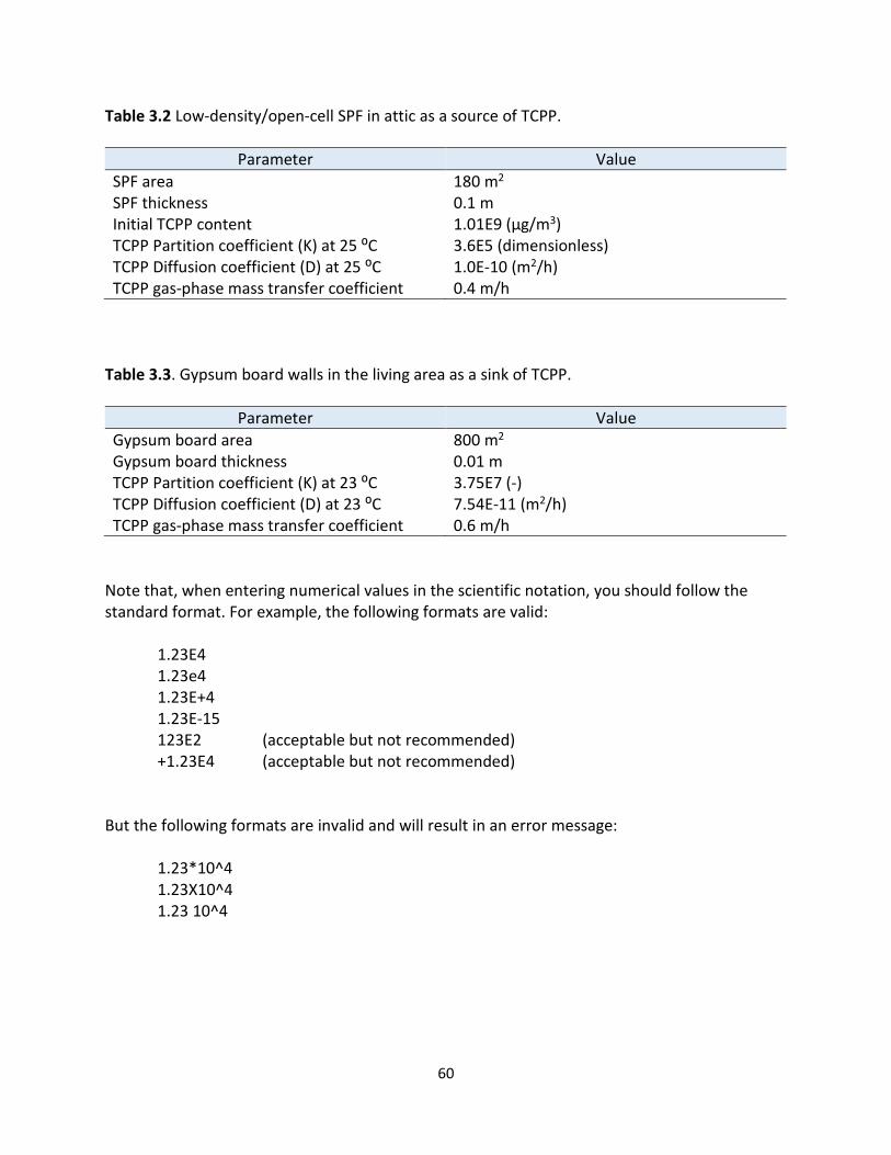
60

Table 3.2 Low-density/open-cell SPF in attic as a source of TCPP.

Parameter Value SPF area 180 m2 SPF thickness 0.1 m Initial TCPP content 1.01E9 (µg/m3) TCPP Partition coefficient (K) at 25 ⁰C 3.6E5 (dimensionless) TCPP Diffusion coefficient (D) at 25 ⁰C 1.0E-10 (m2/h) TCPP gas-phase mass transfer coefficient 0.4 m/h

Table 3.3. Gypsum board walls in the living area as a sink of TCPP.

Parameter Value

Gypsum board area 800 m2 Gypsum board thickness 0.01 m TCPP Partition coefficient (K) at 23 ⁰C 3.75E7 (-) TCPP Diffusion coefficient (D) at 23 ⁰C 7.54E-11 (m2/h) TCPP gas-phase mass transfer coefficient 0.6 m/h

Note that, when entering numerical values in the scientific notation, you should follow the standard format. For example, the following formats are valid:

1.23E4 1.23e4 1.23E+4 1.23E-15 123E2 (acceptable but not recommended) +1.23E4 (acceptable but not recommended)

But the following formats are invalid and will result in an error message:

1.23*10^4 1.23X10^4 1.23 10^4

61

3.3. Create the model 3.3.1 Select building configuration

Launch the SPF program;

If the < a) Air zones > page is not in current view, click the < (1) Building and environment > folder tab and then click the < a) Air zones > page tab.

Click the < Select building configuration > button (Figure 3.1).

Figure 3.1. Creating a new model by clicking button < Select Building Configuration >.

In the next window, click the < With unconditioned zone(s) > radio button located in the “Indoor climate” box at the top-left corner. A drawing showing the living area/attic configuration will appear (Figure 3.2). Click the < Select > button.

62

Figure 3.2. Selecting a building configuration.

Note that if you need a different configuration (e.g., living area/crawlspace or living area/attic/crawlspace), use the < Prev > and < Next > buttons to browse available configurations.

After you have selected a configuration, return to the main window, and enter zone volumes: 300 for living area and 150 for attic (see Figure 3.1 above);

3.3.2 Define air flow matrix

Move to the < b) Ventilation 1 > page by clicking its page tab.

Enter the air flow data shown in Table 3.4 in the air flow matrix table near the upper-left corner of the page (i.e., “Table 1. Normal air exchange flow rates”).

63

Table 3.4. Air flow matrix for the base case with vented attic.

To Zone 0 To Zone 1 To Zone 2 From Zone 0 XXX 150 300 From Zone 1 Calculated XXX 15 From Zone 2 Calculated 15 XXX

3.3.3 Define the source

Click the < (2) Sources > folder tab and then click the < c) Diffusion model > page tab.

To add a new diffusional source, click the < Add > button (Figure 3.3) to bring up the input form for diffusion sources (Figure 3.4).

Figure 3.3. Page < c) Diffusion model > under folder tab < (2) Sources >.

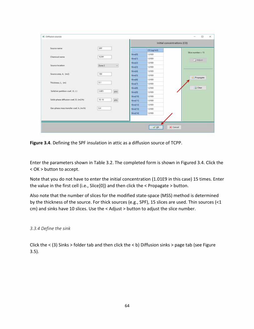
64

Figure 3.4. Defining the SPF insulation in attic as a diffusion source of TCPP.

Enter the parameters shown in Table 3.2. The completed form is shown in Figured 3.4. Click the < OK > button to accept.

Note that you do not have to enter the initial concentration (1.01E9 in this case) 15 times. Enter the value in the first cell (i.e., Slice[0]) and then click the < Propagate > button.

Also note that the number of slices for the modified state-space (MSS) method is determined by the thickness of the source. For thick sources (e.g., SPF), 15 slices are used. Thin sources (<1 cm) and sinks have 10 slices. Use the < Adjust > button to adjust the slice number.

3.3.4 Define the sink

Click the < (3) Sinks > folder tab and then click the < b) Diffusion sinks > page tab (see Figure 3.5).

65

Figure 3.5. Page < b) Diffusion sinks > under folder tab < (3) Sinks >.

Click the < Add > button. The form for diffusional sink is almost identical to that for diffusional sources except that the sink material is divided into 10 slices while sources are divided into 10 or 15 slices depending on the thickness of the material. The completed sink form is shown in Figure 3.6.

66

Figure 3.6. Defining gypsum board walls in living area as a TCPP sink. This form is almost identical to that for diffusion sources except that the number of slices is set to 10.

The distance that a chemical can travel into the sink material, known as the travel distance, is limited for common indoor pollutants and within the timeframe of interest (from a few days to several years). Thus, it is recommended that, for thick sink materials such as brick or concrete walls, the thickness of the sink be set to 0.01 m.

3.3.5 Define simulation conditions

To complete the model, go to the < (7) Simulation conditions > folder. A table for initial air concentrations has already been created. If there are non-zero initial concentrations, enter the values here. For this tutorial, we assume the initial concentrations are all zeros. On the right-side of the screen, select 6 months for simulation duration and 100 for output data points.

Finally, select the output data type by clicking the < Select > button, then choose “1) Air concentrations” and return to the main window (Figure 3.7).

67

Figure 3.7. Completed page < (7) Simulation conditions >.

3.4 Save, compile, inspect, and run the model Save this model to as “MyTCPP-0.IEC”. Click the < Compile > speed button (fifth from left). After successful compilation, click the < Inspect > speed button (sixth from left) to view the compilation results. Click the < Run > speed button (seventh from left) to start the simulation. The results are shown in Figure 3.8.

68

Figure 3.8. Simulation results of model “MyTCPP-0.IEC”.

1.0E+0

1.0E+1

1.0E+2

1.0E+3

0 50 100 150 200

TCPP

Con

cent

ratio

n (µ

g/m

3 )

Elapsed Time (days)

Living area

Attic

69

Tutorial 4: Simulating temperature-dependent TCPP emissions

4.1 Objective

To demonstrate how to define time-varying temperatures in unconditioned zones and temperature-dependent partition and diffusion coefficients. The technical approach to temperature functions are described in Sections 5.4 and 5.6 in the Tester’s Guide.

4.2 Case description

In model “MyTCPP-0.IEC” developed in Tutorial 3, we assumed that the partition and diffusion coefficients for TCPP in the SPF are both constant. In real world, the temperature in the unconditioned zones can vary substantially following diurnal and seasonal patterns. This program allows the user to define the temperature profiles in unconditioned zones and temperature-dependent partition and diffusion coefficients.

We will build the new model from “MyTCPP-0.IEC”. The temperature profile in the attic is simulated as a sine function, as described in Section 5.4.1 in the Tester’s Guide. The input parameters are shown in Table 4.1.

Note that the dates for peak temperature and SPF application must be in the form of mm/dd/yyyy because the sine function considers the leap day (February 29) in a leap year.

Table 4.1. Parameters for the temperature profile in attic.

Parameter Value Temperature function type Sine function (seasonal) Annual average temperature 20 ⁰C Amplitude for seasonal temperature cycle 25 ⁰C Day of the year with highest temperature 07/17/2016 Day of the year for SPF application 05/01/2016

The empirical model for temperature dependence described by Tian et al. (2017) will be used to determine the partition coefficient as a function of temperature (see Section 5.5.1 in the Tester’s Guide for details). Input parameters are shown in Table 4.2.

70

Table 4.2. Parameters for the temperature-dependent partition coefficient for TCPP in SPF.

Parameter Value TCPP-SPF partition coefficient K1 (dimensionless) 3.06E5

Temperature T1 (K) 298.2 Absolute value of slope (a) 0.9 Evaporation enthalpy, ΔHv (J) 8.1E4

The method for estimating the diffusion coefficient as a function of temperature is also from Tien et al. (2016). See Section 5.6.2 in the Tester’s Guide for details. Input parameters are shown in Table 4.3.

Table 4.3. Parameters for the temperature-dependent diffusion coefficient for TCPP in SPF.

Parameter Value Material specific constant (m2/h) 6.05E6 Activation energy, ΔE (J/mol) 9.58E4

4.3 Create the model

Three steps are needed to use the temperature functions:

1. Define the temperature profile; 2. Modify the SPF source to allow K and D to vary with temperature; 3. Define the temperature functions of partition and diffusion coefficients.

4.3.1 Define temperature profile in attic

Open the model “MyTCPP-0.IEC” if it is not currently active.

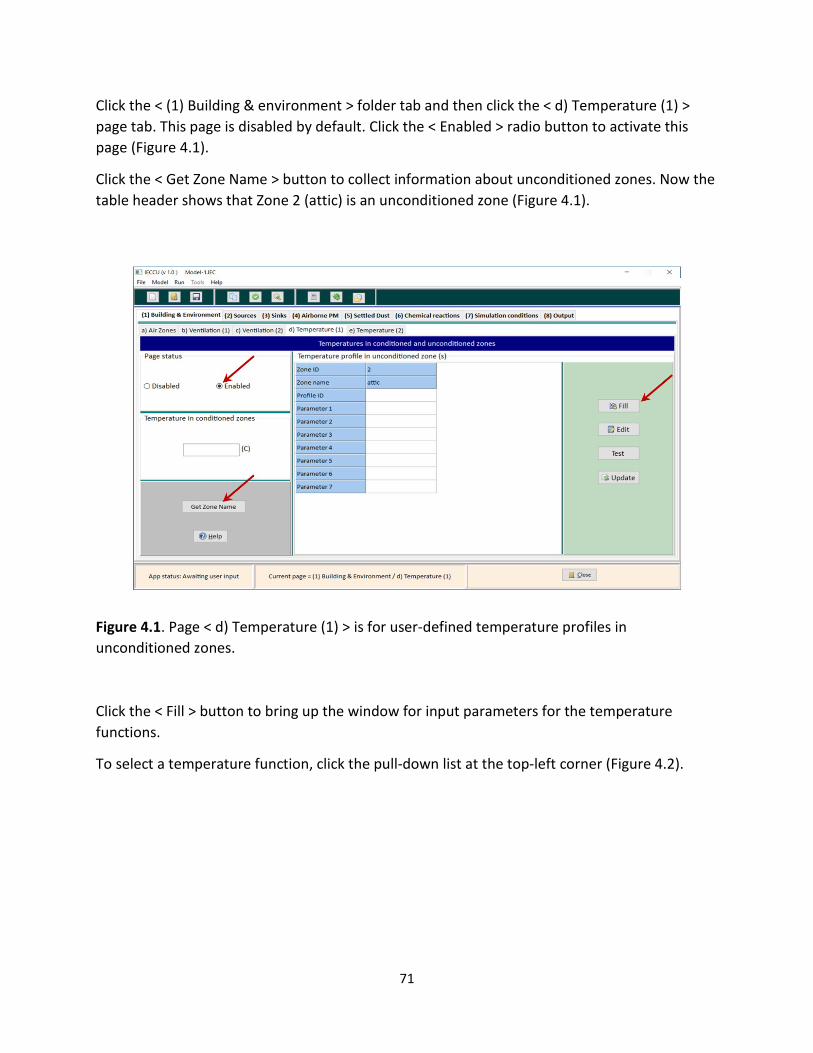
71

Click the < (1) Building & environment > folder tab and then click the < d) Temperature (1) > page tab. This page is disabled by default. Click the < Enabled > radio button to activate this page (Figure 4.1).

Click the < Get Zone Name > button to collect information about unconditioned zones. Now the table header shows that Zone 2 (attic) is an unconditioned zone (Figure 4.1).

Figure 4.1. Page < d) Temperature (1) > is for user-defined temperature profiles in unconditioned zones.

Click the < Fill > button to bring up the window for input parameters for the temperature functions.

To select a temperature function, click the pull-down list at the top-left corner (Figure 4.2).

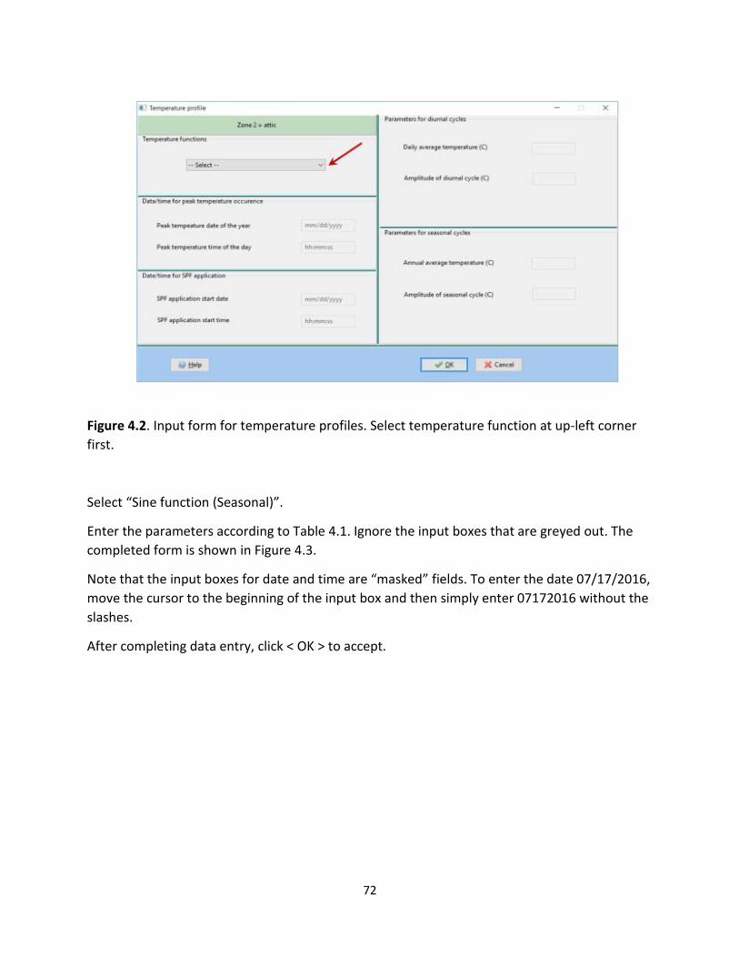
72

Figure 4.2. Input form for temperature profiles. Select temperature function at up-left corner first.

Select “Sine function (Seasonal)”.

Enter the parameters according to Table 4.1. Ignore the input boxes that are greyed out. The completed form is shown in Figure 4.3.

Note that the input boxes for date and time are “masked” fields. To enter the date 07/17/2016, move the cursor to the beginning of the input box and then simply enter 07172016 without the slashes.

After completing data entry, click < OK > to accept.

73

Figure 4.3. Completed input form for the temperature profile in attic.

4.3.2 Modify the SPF source

It takes two steps to define the temperature dependence of partition and diffusion coefficients: (1) modify the SPF source and (2) define the temperature functions.

To modify the SPF source, go to the < c) Diffusion model > page under the < (2) Sources > folder tab.

Click a cell in column 1 in the data table and then click < Edit > (Figure 4.4).

74

Figure 4.4. To make changes to an existing item, click the data column first and then click < Edit >.

In the data entry form for diffusion sources, there is a button next to the input box for partition coefficient with the caption of “f(T)”, which is for “function of temperature”. Click that button. After a confirmation message appears, click < Yes > to confirm the change.

Do the same for the diffusion coefficient. The completed form is shown in Figure 4.5.

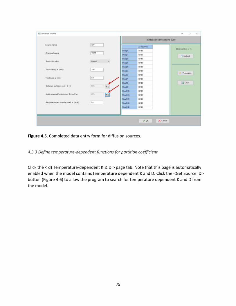
75

Figure 4.5. Completed data entry form for diffusion sources.

4.3.3 Define temperature-dependent functions for partition coefficient

Click the < d) Temperature-dependent K & D > page tab. Note that this page is automatically enabled when the model contains temperature dependent K and D. Click the <Get Source ID> button (Figure 4.6) to allow the program to search for temperature dependent K and D from the model.

76

Figure 4.6. Page < d) Temperature-dependent K & D > is automatically enabled if the model contains temperature-dependent K and D.

To define the temperature function for the partition coefficient, click the < Fill > button on top (see Figure 4.6) to bring up the input form, as shown in Figure 4.7.

Figure 4.7. Temperature function form for partition coefficient.

77

From the box at the top left corner for “Select a method for K”, select “Tian et al. (2017)” by using the pull-down menu.

Enter the values listed in Table 4.4 in the panel on the right side.

Table 4.4. Parameters for the temperature-dependent partition coefficient for TCPP in SPF.

Parameter Value Partition coefficient K1 (-) 3.06E5 (for TCPP / LD/OC SPF) Temperature T1 (K) 298.2 (i.e., 25 ⁰C) Absolute value of slope a 0.9 (See on-screen description on the right) Evaporation enthalpy, dHv (J) 8.1E4 (See on-screen description on the right)

The completed form is shown in Figure 4.8. Click < OK > to accept.

Figure 4.8. Completed temperature function form for partition coefficient.

78

4.3.4 Define temperature-dependent functions for diffusion coefficient

To define the temperature function for diffusion coefficient, click the < Fill > button in the lower part of the screen (See Figure 4.6 above). The temperature function form for diffusion coefficient is similar to that for partition coefficient.

Use the pull-down menu in the “Select a method for D” box at the top-left corner to select “Tian et al. (2017)”.

Enter the values in Table 4.5 the right-side panel:

Table 4.5. Parameters for the temperature-dependent diffusion coefficient for TCPP in SPF.

Parameter Value Material specific constant (m2/h) 6.05E6 Activation energy, ΔE (J/mol) 9.58E4

These parameters give a D value of 1.0E-10 (m2/h) at 25 C for TCPP. The completed form is shown in Figure 4.9. Click the <OK> button to accept.

Figure 4.9. Completed temperature function form for partition coefficient.

79

4.3.5 Select output data types

Click the < (7) Simulation conditions > folder tab. Select “10,000 hours (~1 year)” for simulation duration and 200 for output data points.

Click < Select > and then choose the following output types:

1) Air concentrations, 6) Temperature profiles in unconditioned zone(s), 7) Temperature-dependent partition coef (K), 8) Temperature-dependent diffusion coef (D).

4.4 Save, compile, inspect and run the model

Save the model to file “MyTCPP-1.IEC”.

Compile, inspect and then run the model.

Simulation results are shown in Figures 4.10 through 4.13.

Figure 4.10. Simulated TCPP concentrations in living area and attic with model “MyTCPP-1.IEC”.

0.1

1

10

100

1000

0 100 200 300 400

TCPP

Con

cent

ratio

n (µ

g/m

3 )

Elapsed Time (days)

Living area

Attic

80

Figure 4.11. Simulated air temperature in attic with model “MyTCPP-1.IEC”.

Figure 4.12. Simulated partition coefficient for TCPP-SPF as a function of temperature with model “MyTCPP-1.IEC”.

-20

-10

0

10

20

30

40

50

60

0 50 100 150 200 250 300 350 400

Tem

pera

ture

in a

ttic

(⁰C)

Elapsed Time (days)

July 17, 2016

May 1, 2016

Jan. 15, 2017

1.0E+4

1.0E+5

1.0E+6

1.0E+7

1.0E+8

0 50 100 150 200 250 300 350 400

K (d

imen

sionl

ess)

Elapsed Time (days)

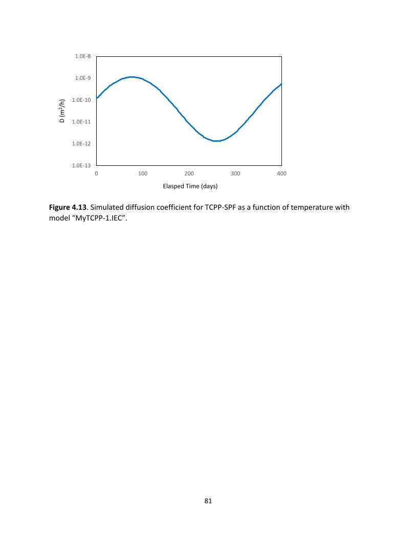
81

Figure 4.13. Simulated diffusion coefficient for TCPP-SPF as a function of temperature with model “MyTCPP-1.IEC”.

1.0E-13

1.0E-12

1.0E-11

1.0E-10

1.0E-9

1.0E-8

0 100 200 300 400

D (m

2 /h)

Elasped Time (days)

82

Tutorial 5: Using the batch mode

5.1 Objective

To demonstrate how to run multiple simulations sequentially unattended. Under the batch mode, the user can run an unlimited number of models. Available simulation modes in IECCU are discussed in Section 3.5 in the Tester’s Guide.

5.2 General steps

Running simulations in batch mode involves four steps:

1. Create an empty folder, 2. Save or copy model files to that folder, 3. Click the < Run batch > speed button, 4. Retrieve simulation results from comma separated value (CSV) files.

5.3 Case description

We have created four models so far. In this practice we will run these four models all together.

5.4 Run batch

5.4.1 Create an empty folder

Create a folder in your hard drive, USB drive, or remote storage device and name it \IEC_batch.

5.4.2 Save or copy model files to that folder

Copy the following four model files to folder \IEC_batch.

• MyModel-1.IEC,

83

• MyModel-2.IEC, • MyTCPP-0.IEC, • MYTCPP-1.IEC.

Note that the last two models have long simulation durations. If you want to save some time from running this tutorial, select shorter durations before moving to next step.

5.4.3 Run batch simulations

Click the < Run batch > speed button (the last from left) (Figure 5.1).

Figure 5.1. Click the < Run batch > speed button to start the simulations in batch mode.

A confirmation message asks whether you need any instructions (Figure 5.2). Click < Yes > to display the help window, or click < No > to bypass this step, or click < Cancel > to exit the batch mode.

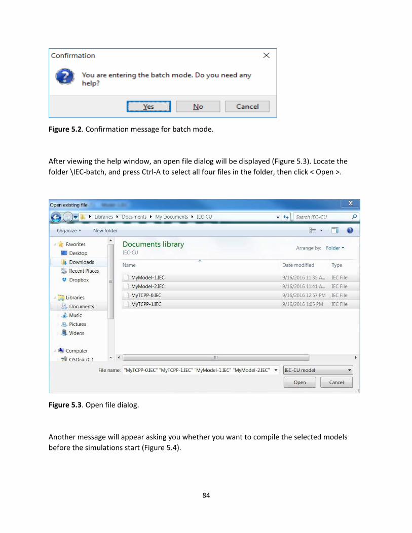
84

Figure 5.2. Confirmation message for batch mode.

After viewing the help window, an open file dialog will be displayed (Figure 5.3). Locate the folder \IEC-batch, and press Ctrl-A to select all four files in the folder, then click < Open >.

Figure 5.3. Open file dialog.

Another message will appear asking you whether you want to compile the selected models before the simulations start (Figure 5.4).

85

Figure 5.4. Confirmation message for optional pre-run compilation.

Click < Yes > to view the compilation report (Figure 5.5).

Figure 5.5. Pre-run compilation report.

86

Click < Continue > to start simulations.

During batch simulations, the status is updated in real time (Figure 5.6).

Figure 5.6. The status window for a batch simulation.

When simulations are completed, a batch report will be displayed (Figure 5.7).

87

Figure 5.7. Batch simulation report.

5.4.4 Retrieve simulation results

Use Windows File Explorer to locate folder \IEC_batch. You can find six CVS files created by the batch simulations. The data can be retrieved by any spreadsheet and database applications. Try to double-click on a file name to open it.

88

Tutorial 6: Gas-phase chemical reactions

6.1 Objective

To demonstrate how to include gas-phase chemical reactions in a model. Representation of gas-phase chemical reactions is discussed in Section 5.10 in the User’s Guide.

6.2 Case description

Methylene diphenyl diisocyanate (MDI) is an aromatic diisocyanate commonly used to manufacture polyurethane. When SPF or polyurethane foam sealant is installed in a home by on-site application, unreacted MDI may be introduced into the air. It is known that isocyanate can react with moisture in air to form amines and carbon dioxide (Equation 1):

RNCO + H2O → RNH2 + CO2 (1)

Note that MDI hydrolysis may be more complex than Equation 1 because MDI contains two isocyanate function groups. As a practical matter, we will treat MDI hydrolysis as an apparent second order process (Equation 2):

MDI + [H2O] → amines (2)

We omit CO2 because it occurs in large volumes in natural air; we placed water vapor in a pair of square brackets because there is an excess amount of water vapor in air and there is no need to track its concentration change over time. We also assume that, after formed, amines remain in air.

The input parameters listed in Table 6.1 are for application of a polyurethane foam sealant in a hypothetical small room. The source emission parameters are from the NRC-CNRC report (Won et al., 2013). The second-order rate constant was roughly estimated from Figure A.4 in the report: the MDI concentration reduced by one half when the relative humidity changed from 0 to 20%. Do not cite this number.

89

Table 6.1. Input parameters for investigating the effect of hydrolytic reaction on MDI concentrations.

Parameter Value Room volume 26 m3 Air change flow 10.9 m3/h (equivalent to 0.42 ach) Source area 0.01 m2

MDI emission factor, E0 153 µg/m2/h (at 40 ⁰C) MDI decay rate constant, k 0.344 h-1 Second-order reaction rate constant at 40 ⁰C 2.5E-24 (cm3/molecule/s) Molecular weight for MDI 250 Molecular weight for amines 224 Relative humidity 20% (at 40 ⁰C)

6.3 Create the model

6.3.1 Define building and ventilation

Select < File > / < New > from the main menu or click the < New > speed button (first from left). Use the default building configuration – a single conditioned zone.

Enter 26 for zone volume.

Click the < b) Ventilation (1) > page tab; locate Table 1 (for normal air exchange flows); enter 10.9 for air flow Q01 (i.e., from Zone 0 to Zone 1).

6.3.2 Define the first-order decay source

Click the < (2) Sources > folder tab and then click the < a) Empirical models > page tab.

Click the < Add > button.

In the input form for empirical sources, select model (12) First-order decay.

Enter the values in the required field (Figure 6.1). Click < OK >.

90

Figure 6.1. Representing MDI emission by the first-order decay source model.

6.3.3 Define the chemical reaction

Click the < (6) Chemical reactions > folder tab; click the < Add > button to bring up the input form for chemical reactions.

Enter or select the values listed in Table 6.2.

Table 6.2. Input parameters for chemical reactions.

Parameter Value Reaction order Second order Type of rate constant (k) K=constant Value of rate constant 2.5 x 10-24

Reactant A MDI Reactant B [H2O] Number of reaction products 1 Yield 1 1 Product 1 amines

91

The completed form is shown in Figure 6.2. Click < OK > to return to the main window.

Figure 6.2. Completed input form for chemical reactions.

Locate the molecular weight table on page < (6) Chemical reactions >; enter 250 for MDI and 224 for RNH2.

At the bottom-right corner, enter 20 for relative humidity and 40 for temperature.

The completed page is shown in Figure 6.3.

92

Figure 6.3. Completed page for chemical reactions.

6.3.4 Define simulation conditions

Click the < (7) Simulation conditions > folder tab. Set simulation duration to 10 hours and output data points to 50. Then select 1) Air concentrations for output.

6.4 Save, compile, inspect and run the model

Save the model to MyMDI-1.IEC.

Compile and then inspect the model.

Run the model.

The results are shown in Figure 6.4. Note that the rate constant was estimated from experimental data at 40⁰C and no adjustments were made for the simulation.

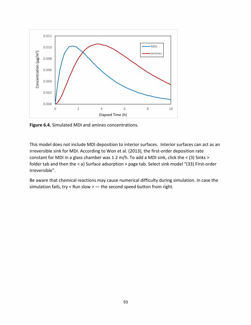
93

Figure 6.4. Simulated MDI and amines concentrations.

This model does not include MDI deposition to interior surfaces. Interior surfaces can act as an irreversible sink for MDI. According to Won et al. (2013), the first-order deposition rate constant for MDI in a glass chamber was 1.2 m/h. To add a MDI sink, click the < (3) Sinks > folder tab and then the < a) Surface adsorption > page tab. Select sink model “(33) First-order irreversible”.

Be aware that chemical reactions may cause numerical difficulty during simulation. In case the simulation fails, try < Run slow > — the second speed button from right.

0.000

0.002

0.004

0.006

0.008

0.010

0.012

0 2 4 6 8 10

Conc

entr

atio

n (µ

g/m

3 )

Elapsed Time (h)

MDI

amines

94

Tutorial 7: TCPP interactions with airborne particulate matter (PM)

7.1 Objective

To demonstrate how to include airborne PM in a model. Technical approach to modeling SVOC interactions with airborne PM is given in Section 5.8 in the Tester’s Guide.

7.2 Case description

As shown in Figure 4.10 above, the yearly average TCPP concentration in the living area is 2.7 µg/m3. We would like to estimate the particle-phase concentration for TCPP by assuming the conditions in Table 7.1.

Table 7.1. Assumed properties for airborne PM. Parameter Value Particle size 2.5 µm Particle density 1 g/cm3 Outdoor PM mass concentration 30 µg/m3 TCPP concentration in outdoor PM 0 µg/g Initial PM mass concentration in living area 14.4 µg/m3 Initial PM mass concentration in attic 25.1 µg/m3 Particle-air partition coefficient for TCPP [1] 1E6 (dimensionless) PM penetration factor 0.8 PM deposition rate constant in attic 0.60 PM deposition rate constant in living area 0.65

[1] The dimensionless particle-air partition coefficient is defined as Cp/Ca at equilibrium, where Cp and Ca are the chemical concentrations in the particles and air, respectively, in the units of (µg TCPP/m3 dust).

7.3. Create the model

7.3.1 Open model MyTCPP-1.IEC

We will build this model by adding the PM component to the model you previously created in Tutorial 1 (default file “MyTCPP-1.IEC”).

95

To open this model, click the < Open > speed button (second from left) to load MyTCPP-1.IEC.

7.3.2 Define airborne PM

Click the < (4) Airborne PM > folder tab to access the two input tables for PM, as shown in Figure 7.1.

Figure 7.1. Under the < (4) Airborne PM > folder tab, there are two pages: < a) Airborne PM > (shown) and < b) Airborne PM (cont) >.

Enter chemical name “TCPP” in the box near the top-right corner.

Click the < Add > button to bring up the input form for PM.

Enter the required parameters according to Table 7.1. The completed form is shown in in Figure 7.2.

Click < OK > to return to the main window.

96

Figure 7.2. Input form for PM properties.

7.3.3 Define deposition rate constants and initial PM mass concentrations

Click the < b) Airborne PM (cont) > page tab. There are two tables on this page. They are for, PM deposition rate constants (top) and initial mass concentrations of indoor PM (bottom). Enter the input data, as shown in Figure 7.3.

97

Figure 7.3. Completed < b) Airborne PM (cont) > page.

7.3.4 Select output data types

Click the < (7) Simulation conditions > folder tab; click the < Select > button to choose the following output types:

1) Air concentrations, 2) Chemical concentrations in airborne PM (µg/m3 air), 3) Chemical concentrations in airborne PM (µg/g PM), 4) Mass concentration of airborne PM (µg/m3 air).

The completed page is shown in Figure 7.4.

98

Figure 7.4. Completed simulation conditions page. Output selection includes three types of PM data.

99

7.4 Save, compile, inspect, and run the model

Save the new model to file “MyTCPP-PM.IEC”.

Compile, inspect and then run the model.

The results are shown in Figure 7.5.

Figure 7.5. Simulated particle-phase TCPP concentrations.

0.1

1

10

100

1000

0 50 100 150 200 250 300 350 400

TCPP

in p

rtic

le-p

hase

(µg/

g)

Time (days)

Attic

Living area

100

Tutorial 8: TCPP interactions with settled dust

8.1 Objective

To demonstrate how to include settled dust in a model. Technical approach to modeling SVOC interactions with airborne PM is given in Section 5.8 in the Tester’s Guide.

8.2 Case description

In this tutorial, we will use the model you created in the previous section: MyTCPP-PM.IEC. Additional parameters are shown in Table 8.1:

Table 8.1. Assumed properties for settled dust in living area (zone 1).

Parameter Value Surface area 120 m2 Dust loading 5 g/m2 Dust size 50 µm Dust density 1.2 g/cm3 Dust-air partition coefficient 1E6 Gas-phase mass transfer coefficient for TCPP/dust 5 m/h Initial TCPP concentration in dust 0 µg/g

8.3 Create the model 8.3.1 Load model MyTCPP-PM.IEC

Open file TCPP-PM.IEC if it is not currently active.

8.3.2 Define settled dust

Click the < (5) Settled dust > folder tab.

101

Click the < Add > button to bring up the input form for settled dust (Figure 8.1). Give the dust a name, e.g., “D50”; select “Zone 1” for location; enter 50 for dust diameter and 1.2 for density. Now the form should look like Figure 8.1.

Figure 8.1. Input form for settled dust prior to calculating dust number. Parameter “Dust number” is a calculated field. Click the button next to it (See Figure 8.1) to display the calculation sheet (Figure 8.2). Note that, dust diameter and density have already been copied to the sheet. Enter values on the left side of Figure 8.2 and then click the < Calculate > button. Now the value “1.146E10” should appear in the box for “Dust number”. Click the < Paste > button to go back to the main window.

102

Figure 8.2. Calculation sheet for dust number. Finish the right-side of input form for dust. The completed form is shown in Figure 8.3. Click < OK > to return to the main window. Now the < (5) Settled dust > page should look like Figure 8.4.

103

Figure 8.3. Completed data entry form for settled dust.

Figure 8.4. Completed < (5) Settled dust > page.

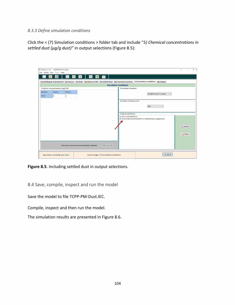
104

8.3.3 Define simulation conditions Click the < (7) Simulation conditions > folder tab and include “5) Chemical concentrations in settled dust (µg/g dust)” in output selections (Figure 8.5):

Figure 8.5. Including settled dust in output selections. 8.4 Save, compile, inspect and run the model Save the model to file TCPP-PM-Dust.IEC. Compile, inspect and then run the model.

The simulation results are presented in Figure 8.6.

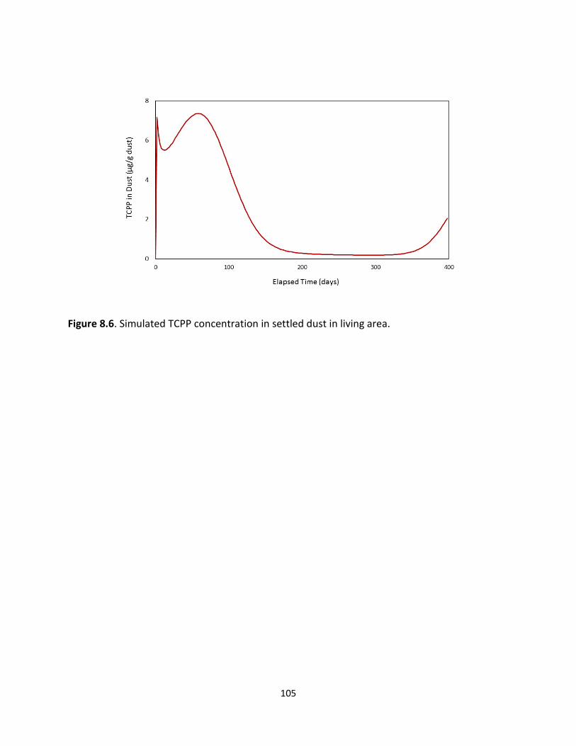
105

Figure 8.6. Simulated TCPP concentration in settled dust in living area.

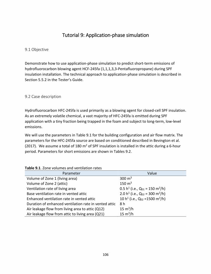
106

Tutorial 9: Application-phase simulation

9.1 Objective

Demonstrate how to use application-phase simulation to predict short-term emissions of hydrofluorocarbon blowing agent HCF-245fa (1,1,1,3,3-Pentafluoropropane) during SPF insulation installation. The technical approach to application-phase simulation is described in Section 5.5.2 in the Tester’s Guide.

9.2 Case description

Hydrofluorocarbon HFC-245fa is used primarily as a blowing agent for closed-cell SPF insulation. As an extremely volatile chemical, a vast majority of HFC-245fa is emitted during SPF application with a tiny fraction being trapped in the foam and subject to long-term, low-level emissions.

We will use the parameters in Table 9.1 for the building configuration and air flow matrix. The parameters for the HFC-245fa source are based on conditioned described in Bevington et al. (2017). We assume a total of 180 m2 of SPF insulation is installed in the attic during a 6-hour period. Parameters for short emissions are shown in Tables 9.2.

Table 9.1. Zone volumes and ventilation rates Parameter Value

Volume of Zone 1 (living area) 300 m3 Volume of Zone 2 (attic) 150 m3 Ventilation rate of living area 0.5 h1 (i.e., Q01 = 150 m3/h) Base ventilation rate in vented attic 2.0 h1 (i.e., Q02 = 300 m3/h) Enhanced ventilation rate in vented attic 10 h1 (i.e., Q02 =1500 m3/h) Duration of enhanced ventilation rate in vented attic 8 h Air leakage flow from living area to attic (Q12) 15 m3/h Air leakage flow from attic to living area (Q21) 15 m3/h

107

Table 9.2. Parameters for short-term HFC245fa emissions Parameter Value

Location of SPF insulation Attic SPF area 180 m2 HCF245fa content formulation (M0) 2.55E8 µg/m2 First-order decay rate constant for short-term HFC245fa emission (k)

1 h-1

Application duration 6 hours

9.3 Create the model

9.3.1 Define building configuration

Click the < New > speed button (the first from left).

Click the < Select building configuration > button, then select the living area – attic configuration.

Enter zone volumes.

9.3.2 Define air flow matrices for base and enhanced ventilation

Click the < b) Ventilation (1) > page tab, then enter the values in Tables 9.3 and 9.4 to Tables 1 and 2 on the screen. Before entering the data for enhanced ventilation, activate Table 2 by clicking < Enabled > in the “Table 2 status” box. After finishing the tables, enter the start and finish times (0 and 8 hours) for enhanced ventilation.

Table 9.3. Air flow matrix for base ventilation

To Zone 0 To Zone 1 To Zone 2 From Zone 0 XXX 150 300 From Zone 1 Calculated XXX 15 From Zone 2 Calculated 15 XXX

108

Table 9.4. Air flow matrix for enhanced ventilation during first 8 hours

To Zone 0 To Zone 1 To Zone 2 From Zone 0 XXX 150 1500 From Zone 1 Calculated XXX 15 From Zone 2 Calculated 15 XXX

9.3.3 Define application-phase model

Click the < (2) Sources > folder tab and then click the < b) Application phase > page tab.

Click the < Add > button to bring up the input form for application-phase simulation.

To select an emission model, click the box near the top-left corner (Figure 9.1).

Select model “(22) First-order decay”. Then enter the parameters as required (Figure 9.2).

Figure 9.1. Input form for application-phase simulation.

109

Figure 9.2. Input form for application-phase simulation after the emission model is selected and parameters entered.

9.3.4 Define simulation conditions

Click the < (7) Simulation conditions > folder tab; enter 20 hours for simulation duration and 100 for output data points.

For output data types, select “1) Air concentrations”.

9.4 Save, compile, inspect and run the model

Save this model to “HFC-245fa.IEC”.

Compile, inspect, and then run the model. The results are shown in Figure 9.3.

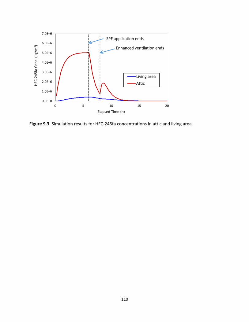
110

Figure 9.3. Simulation results for HFC-245fa concentrations in attic and living area.

0.0E+0

1.0E+6

2.0E+6

3.0E+6

4.0E+6

5.0E+6

6.0E+6

7.0E+6

0 5 10 15 20

HFC-

245f

a Co

nc. (

µg/m

3 )

Elapsed Time (h)

Living areaAttic

SPF application ends

Enhanced ventilation ends

111

Tutorial 10: Importing indoor-outdoor and zone-to-zone air flow data

10.1 Objective

To demonstrate how to import air flow data from a comma separated values (CSV) file generated by other models. Representation of indoor-outdoor and zone-to-zone air flows in IECCU is described in Section 5.3 in the Tester’s Guide.

10.2 Case description

In this tutorial we will use the MyModel-1.IEC, which you created in Tutorial 1 and is for a constant source in a single zone with a constant air change rate. We will replace the constant air change flows with a set of dummy air flow data stored in file “Dummy air flows.CSV”, which is downloadable from the Secure File Sharing Website (Figure 10.1).

Figure 10.1. Hypothetical air exchange flow from file “Dummy temperatures.CSV”.

10.3 Create the model

Open the file MyModel-1.IEC.

0

10

20

30

40

50

0 5 10 15 20

Flow

Rat

e (m

3 /h)

Elapsed Time (h)

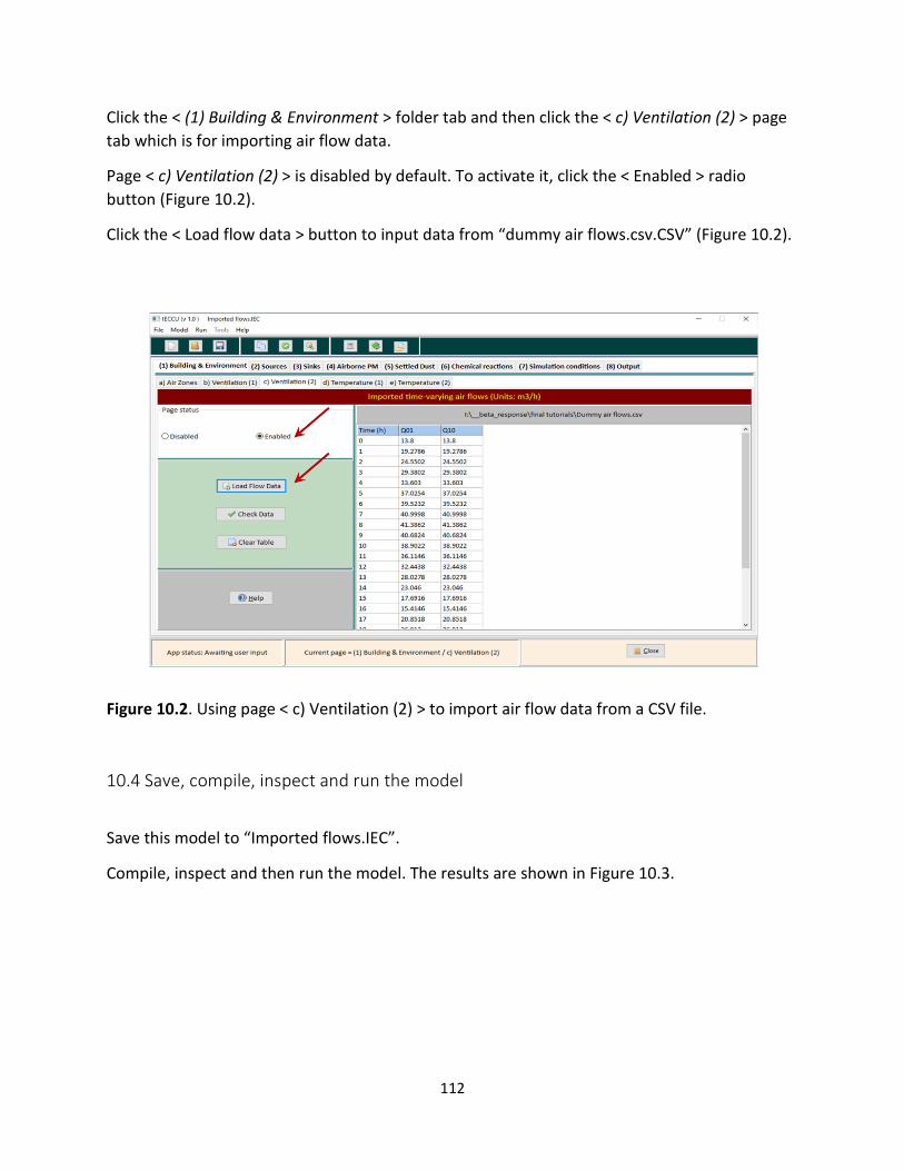
112

Click the < (1) Building & Environment > folder tab and then click the < c) Ventilation (2) > page tab which is for importing air flow data.

Page < c) Ventilation (2) > is disabled by default. To activate it, click the < Enabled > radio button (Figure 10.2).

Click the < Load flow data > button to input data from “dummy air flows.csv.CSV” (Figure 10.2).

Figure 10.2. Using page < c) Ventilation (2) > to import air flow data from a CSV file.

10.4 Save, compile, inspect and run the model

Save this model to “Imported flows.IEC”.

Compile, inspect and then run the model. The results are shown in Figure 10.3.

113

Figure 10.3. Simulation results from models “Imported flows.IEC” (the blue curve) and “MyModel-1.IEC” (the red curve).

0

2

4

6

0 5 10 15 20

Conc

entr

atio

n (µ

g/m

3 )

Elapsed Time (h)

w/ imported air flows

w/ constant air flows

114

Tutorial 11: Importing indoor temperature data

11.1 Objective

To demonstrate how to import temperature data generated by other models. Representation of indoor temperatures in unconditioned zones is described in Section 5.4 in the Tester’s Guide.

11.2 Case description

We will build this model by modifying the file “MyTCPP-1.IEC”, in which the temperature profile in the attic is defined by the user. In this tutorial, we will import hypothetical temperature profiles from file “Dummy temperatures.CSV” (See Figure 11.1).

Figure 11.1. Hypothetical temperature profile in attic from file “Dummy temperatures.CSV”.

20

25

30

35

40

45

50

55

0 500 1000 1500 2000 2500 3000

Tem

pera

ture

in A

ttic

(⁰C)

Elapsed Time (h)

115

11.3 Create the model

Open the file “MyTCPP-1.IEC”.

Click the < e) Temperature (2) > page tab.

Click the < Enabled > radio button to activate this page (Figure 11.2). Note that, if page < e) Temperature (2) > is enabled, < d) Temperature (1) > will be disabled.

Click the < Load temperature data > button to open the file “Dummy temperatures.CSV”.

Figure 11.2. Page < e) Temperature (2) > after loading data from file “Dummy temperatures”.

Click the < (7) Simulation conditions > folder tab; change simulation duration to 100 days.

11.4 Save, compile, inspect and run the model

Save this model to file “MyTCPP-T-file.IEC”.

Compile, inspect and then run the model. The results are shown in Figures 11.3 and 11.4.

116

Figure 11.3. Simulated TCPP concentration in attic.

Figure 11.4. Simulated TCPP concentration in living area.

0

200

400

600

800

0 500 1000 1500 2000 2500

TCPP

in a

ttic

(µg/

m3 )

Elapsed Time (h)

0

5

10

15

20

0 500 1000 1500 2000 2500

TCPP

in li

ving

are

a (µ

g/m

3 )

Elapsed Time (h)

117

Tutorial 12: Including an HVAC system

12.1 Objective To demonstrate how to include an HVAC system in the model.

12.2 Case description In this tutorial, we will use the case described in Tutorial 3 — TCPP emissions from SF applied in attic. The only change is that there is an HVAC system in the attic. As shown in Figure 12.1, air flows Q13, Q31, Q23 and Q32 represent, respectively, return air, supply air, air leakage from attic into the HVAC system, and air leakage from the HVAC system into attic. Because the TCPP source is located in the attic, the magnitude of the “leak-in” flow — Q23 — has the most significant effect on the contaminant concentration in the living area.

Figure 12.1. Air zones and interzone air flows for modeling TCPP emission from SPF applied in attic, where the HVAC system is located.

118

IECCU treats the HVAC system as a special air zone. The volumes of the three zones are shown in Table 12.1. In this tutorial, we set both the supply and return air flows (Q31 and Q13) to 1500 m3/h. We also assume that the leak-in (Q23) and leak-out (Q32) flows are both 150 m3/h (Table 12.2). Other interzonal air flows are the same as those in Tutorial 3.

Table 12.1. Zone names and volumes for Tutorial 12.

Zone ID Zone Name Volume (m3) 1 LvArea 300 2 Attic 150 3 HVAC 2.5

Table 12.2. Interzonal air flows for Tutorial 12 (Unit: m3/h)

To zone 0 To zone 1 To zone 2 To zone 3 From zone 0 XXX 150 300 0 From zone 1 Calculated XXX 15 1500 From zone 2 Calculated 15 XXX 100 From zone 2 Calculated 1500 100 XXX

Note that the air flows moving in and out of the HVAC system (Q13, Q23, Q31, and Q32) are those when the system is running. Because the HVAC switches frequently between on and off, the simulation uses the time-averaged air flows, which are obtained by multiplying the HVAC flow rates in Table 12.2 by the time fraction with the system turned on. In this tutorial, we assume the HVAC is turned on 25% of the time. Thus, for example, the time-averaged return flow is Q13 = 1500 × 25% = 375 m3/h.

12.3 Create the model Open the model you created in Tutorial 3 (“MyTCPP-0.IEC”). To add the HVAC system to attic, click the <Select Building Configuration> button on the first page under folder < (1) Building & Environment > (Figure 12.2).

119

Figure 12.2. The building configuration for Tutorial 3. Click the <Select Building Configuration> button to add the HVAC system.

In the next window, click on <With unconditioned zones> in the “Indoor climate” box. Select <Yes> in the “Include the HVAC?” box, then enter 25 in the “Time fraction with HVAC on” box (Figure 12.3).

Figure 12.3. Adding the HVAC system to the building configuration. If the configuration shown in the image is not the one you want, use the <Prev> and <Next> buttons to browse the options.

120

Click the <Select> button to return to the main window. Now the model has three zones: LvArea, attic, and HVAC (Figure 12.4). Note that the user must enter the zone volumes (Table 12.1) after changing the building configuration.

Figure 12.4. The new building configuration includes the HVAC as the third zone. The time fraction with the HVAC-on is 25%.

Now turn to page < b) Ventilation (1) >. Click the <Select HVAC> button to specify the location of the HVAC (Figure 12.5).

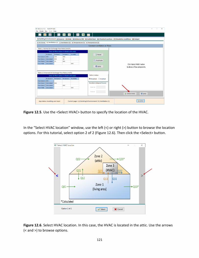
121

Figure 12.5. Use the <Select HVAC> button to specify the location of the HVAC.

In the “Select HVAC location” window, use the left (<) or right (>) button to browse the location options. For this tutorial, select option 2 of 2 (Figure 12.6). Then click the <Select> button.

Figure 12.6. Select HVAC location. In this case, the HVAC is located in the attic. Use the arrows (< and >) to browse options.

122

Finally, fill out the blank cells in the flow matrix at the top-left corner in page < b) Ventilation (1) > with the data in Table 12.2 above. The completed page is shown in Figure 12.7.

Figure 12.7. Completed page < b) Ventilation (1) >.

Note that, adding the HVAC system to model MyTCPP-0.IEC affects only building configuration and air flow matrix. It does not affect the information in other pages.

Save the new model to file “MyTCPP-HVAC.IEC”.

12.4 Compile and run the model

Compile and then run the model. The simulated TCPP concentration in the living area is shown in Figure 12.8 (the red curve). The elevated concentration was caused by the leak-in flow (Q23) in Figure 12.1.

123

Figure 12.8. The effect of the HVAC system on the simulated TCPP concentrations in the living area. The blue curve is from Tutorial 3. When the HVAC is in the source zone, the leak-in air flow increases the chemical concentration in the conditioned zones.

0

5

10

15

20

0 50 100 150 200

TCPP

Con

cent

ratio

n (µ

g/m

3 )

Elapsed Time (days)

No HVAC

With HVAC

124

References

Bevington, C., Guo, Z., Hong, T., Hubbard, H., Wong, E., Sleasman, K., and Hetfield, H. (2017). A modeling approach to quantify exposures from emissions of spray polyurethane foam insulation in indoor environments. In: ASTM Special Technical Publication 1589 – On Developing Consensus Standards for Measuring Chemical Emissions from Spray Polyurethane Foam (SPF) Insulation, pp 199-227.

Won, D., Nong, G., Lusztyk, E., and Schleibinger, H. (2013). Emissions of MDI from do-it-yourself products. NRC-CNRC Institute for Research and Construction, Canada. Report A1-002093.