PROGRAMMABLE FORCE FIELDS FOR DISTRIBUTED

MANIPULATION, AND THEIR IMPLEMENTATION USING

MICRO-FABRICATED ACTUATOR ARRAYS

A Dissertation

Presented to the Faculty of the Graduate School

of Cornell University

in Partial Ful�llment of the Requirements for the Degree of

Doctor of Philosophy

byKarl-Friedrich B�ohringer

August 1997

c Karl-Friedrich B�ohringer 1997

ALL RIGHTS RESERVED

PROGRAMMABLE FORCE FIELDS FOR DISTRIBUTED MANIPULATION, ANDTHEIR IMPLEMENTATION USING MICRO-FABRICATED ACTUATOR ARRAYS

Karl-Friedrich B�ohringer, Ph.D.Cornell University 1997

Programmable force vector �elds can be used to control a variety of exible planarparts feeders such as massively-parallel micro actuator arrays or transversely vibrating(macroscopic) plates. These new automation designs promise great exibility, speed, anddexterity|they may be employed to position, orient, singulate, sort, feed, and assembleparts.

A wealth of geometric and algorithmic problems arise in the control and programmingof manipulation systems with many independent actuators. The theory of programmableforce �elds represents the �rst systematic attack on massively-parallel distributed manipu-lation based on geometric and physical reasoning. We show how to develop combinatoriallyprecise planning algorithms that synthesize force �eld strategies for controlling a very largenumber of distributed actuators in a principled, geometric, task-level fashion.

When a part is placed on our devices, the programmed force �eld induces a force andmoment upon it. Over time, the part may come to rest in a dynamic equilibrium state.By chaining together sequences of force �elds, the equilibrium states of a part in the �eldmay be cascaded to obtain a desired �nal state. The resulting strategies require no sensingand enjoy e�cient planning algorithms.

This thesis introduces new experimental devices that can implement programmableforce �elds. In particular, we describe the M-Chip (Manipulation Chip), a massively-parallel array of programmable micro-motion pixels. Both the M-Chip, as well as macro-scopic devices such as transversely vibrating plates, may be programmed with force �elds,and their behavior predicted and controlled using our equilibrium analysis. We demon-strate lower bounds (i.e., impossibility results) on what the devices cannot do, and resultson a classi�cation of control strategies yielding design criteria by which well-behaved ma-nipulation strategies may be developed. We de�ne composition operators to build complexstrategies from simple ones, and show the resulting �elds are also well-behaved.

Finally, we consider parts feeders that can only implement a very limited \vocabulary"of force �elds. We show how to plan and execute parts-posing and orienting strategies forthese devices, but with a signi�cant increase in planning complexity and some sacri�cein completeness guarantees. We discuss the tradeo� between mechanical complexity andplanning complexity.

Biographical Sketch

Karl-Friedrich B�ohringer was born in Freudenstadt, Germany and grew up in the BlackForest town of Baiersbronn. He attended the Technical University of Karlsruhe as a studentin computer science, and graduated with the degree of Diplom-Informatiker. He thenjoined Cornell University in Ithaca, New York to pursue a doctorate degree. During hisgraduate studies, he spend a year as a Visiting Scholar at the Robotics and the TransducersLaboratories at Stanford University. After receiving his Ph.D. in computer science, he

departed Cornell for a postdoctoral researcher position at the University of California atBerkeley.

iii

Acknowledgements

This thesis, and the part of my life that I spent working on it, has been largely in uencedand supported by many people who were of immeasurable help and inspiration to me. Mythesis advisor and committee chair, Bruce Randall Donald, has been a never-ending sourceof new ideas. He has provided me with support and guidance throughout my time as agraduate student. In many exciting conversations, my advisor Noel C. MacDonald hasgiven me vision, determination, and optimism. Thanks also to my committee members

Daniel Huttenlocher and Pradeep Chintagunta whose continuing help and advice I greatlyappreciated.

The following is hardly a complete list of people who have all contributed to this thesis| I am very grateful for their ideas and help: Tamara Lynn Abell, Eric Babson, VivekBhatt, John Canny, Bernard Chazelle, Paul Chew, Perry Cook, Subhas Desa, Mike Erd-mann, Steve Glander, Ken Goldberg, Danny Halperin, Srikanth Kannapan, Lydia Kavraki,Greg Kovacs, Jean-Claude Latombe, Matt Mason, Al Rizzi, Ivelisse Rubio, Andy Ruina,Ken Steiglitz, John Suh, and Andy Yao. Thanks especially to Jean-Claude Latombe andGreg Kovacs for their hospitality during my stay at their labs at Stanford University.

MEMS fabrication would have been impossible for a \theorist" without the help of thesta� and students at the Cornell Nanofabrication Facility, in particular the MacDonaldgroup members Scott Adams, Arturo Ayon, Liang Chen, Jon Das, Dan Haronian, Wolf-gang Hofmann, Trent Huang, Ali Jazairy, Rob Mihailovich, Scott Miller, Ikuo Ogo, RamaPrasad, Bryan Reed, Taher Saif, Kevin Shaw, Russ Webb, Peter Kenji Yamasaki, andYang Xu.

My fellow roboticists at the Cornell Robotics & Vision Lab, Amy Briggs, Russell Brown,Jim Jennings, Dinesh Pai, Jonathan Rees, Daniela Rus, Pat Xavier, as well as Vivek Bhattand Ken Goldberg have all contributed to a creative and productive environment for myresearch.

Greg Kovacs and John Suh at the Transducers Lab, Stanford University were greatcolleagues who generously made their micro cilia chips available to us.

Thanks to Bruce Land, Chris Pelkie, and Martin Berggren at the Cornell Theory Center- Scienti�c Visualization for their help in preparing videos and animations, and for givingus access to the latest developments and tools for digital image and video processing.

Support for our robotics research was provided in part by the National Science Foun-dation (NSF) under grants IRI-8802390, IRI-9000532, IRI-9201699, and by a PresidentialYoung Investigator award to Bruce Donald, in part by an NSF/ARPA Small Grant forExploratory Research IRI-9403903, and in part by the AFOSR, the Mathematical SciencesInstitute, Intel Corporation, and AT&T Bell laboratories. This work was supported by

iv

ARPA under contract DABT 63-69-C-0019. All fabrication of single-crystal silicon actu-ator arrays was performed at the Cornell Nanofabrication Facility at Cornell Universitywhich is supported by ARPA, NSF, and Industrial A�liates.

*

During my stay at Cornell, I was lucky to meet truly special people, who have been withme at all times. Hoai Huong Tran supported me in any possible way. My friend VivekBhatt has shared and given so much to me | thank you! The same is true for ErrolMontes-Pizarro and Hideki \Trip" Suzuki.

I am in�nitely grateful to our great teacher Errol Montes-Pizarro, as well as to KjartanStefansson, Hoai Huong Tran, and all those who spent many late nights with me playingthe literally divine game of Dominoes.

I thank Vivek Bhatt, Hideki \Trip" Suzuki, Andrew Davidson, and all the other rockclimbers for low-gravity days at the Lindseth climbing wall, the Gunks, Joshua Tree, thestill unconquered Grumman Wall, and the Chariot's.

Thanks to my Tae Kwon Do instructors Sandy Glattner, Raphael Gilbert, Mary Wim-satt, Grand Master Duk Sun Son, and to all the members of our do-jo.

Thanks also to my house mates in the Cornell golf course, in the famous Albany StreetHouse, on Slaterville Road, in Cascadilla Park, on Maple Hill, and on University Avenue.

Daniel Scharstein provided good ideas and conversation in various German dialects {�a'di! My o�ce mates Michael Slifker, Richard Chapman, Takako Hickey, and Rick Aaronhave kept me in good company while at work. Thanks to my o�ce neighbor Aswin vanden Berg for his excellent selection of music, bringing to life the Cornell computer sciencedepartment on lonely weekend nights.

Jan Batzer, Jessie Dimick, Linda Mardel, and Debbie Smith have all helped me a lotin dealing with Cornell bureaucracy and administration.

Finally, I am indebted to my roots back home in Baiersbronn, Germany, which includeBent Beilharz, Roman Husz, Markus Kieninger, Mirco Rizutto, Dirk Schmid, the Daunoras

family and all other friends, and my family (includng my new nephew Manuel).Thanks to \KK" Krishnamurty Kambhampati, Gisela Leclere and Mostafa from Mo-

rocco, Filippo Tampieri, Jennifer Thambayah, Lien Tran, and Mona Matar for a goodstart, and to Vivek Bhatt and Angelina Kalianda for a good �nish at Cornell.

v

Table of Contents

1 Introduction 11.1 Parts Feeders . . . . . . . . . . . . . . . . . . . . . . . . . . . . . . . . . . 4

1.1.1 Microfabricated Actuator Arrays . . . . . . . . . . . . . . . . . . . 61.1.2 Macroscopic Vibratory Parts Feeders . . . . . . . . . . . . . . . . . 9

2 Equilibrium Analysis For Programmable Vector Fields 112.1 Squeeze Fields and Equilibria . . . . . . . . . . . . . . . . . . . . . . . . . 112.2 Polygon Bisectors and Complexity . . . . . . . . . . . . . . . . . . . . . . . 132.3 Planning of Manipulation Strategies . . . . . . . . . . . . . . . . . . . . . . 202.4 Example: Uniquely Orienting Rectangular Parts . . . . . . . . . . . . . . . 232.5 Relaxing the 2Phase Assumption . . . . . . . . . . . . . . . . . . . . . . . 27

3 Lower Bounds: What Programmable Vector Fields Cannot Do 293.1 Unstable Fields . . . . . . . . . . . . . . . . . . . . . . . . . . . . . . . . . 293.2 Unstable Parts . . . . . . . . . . . . . . . . . . . . . . . . . . . . . . . . . 30

4 Completeness: Classi�cation Using Potential Fields 334.1 Properties of Lifted Force and Potential Fields . . . . . . . . . . . . . . . . 374.2 Examples: Classi�cation of Force Fields . . . . . . . . . . . . . . . . . . . . 394.3 Upward-Shaped Potential Fields . . . . . . . . . . . . . . . . . . . . . . . . 43

4.3.1 Elementary De�nitions . . . . . . . . . . . . . . . . . . . . . . . . . 434.3.2 Equilibrium Criterion . . . . . . . . . . . . . . . . . . . . . . . . . . 44

5 New and Improved Manipulation Algorithms 465.1 Radial Strategies . . . . . . . . . . . . . . . . . . . . . . . . . . . . . . . . 465.2 Manipulation Grammars . . . . . . . . . . . . . . . . . . . . . . . . . . . . 51

5.2.1 Finite Field Operators . . . . . . . . . . . . . . . . . . . . . . . . . 515.2.2 Example: Uniquely Posing Planar Parts . . . . . . . . . . . . . . . 535.2.3 Summary . . . . . . . . . . . . . . . . . . . . . . . . . . . . . . . . 60

6 Experimental Apparatus for Programmable Force Fields 626.1 Microfabricated Arrays of Single-Crystal Silicon Torsional Actuators . . . . 62

6.1.1 Actuator Design . . . . . . . . . . . . . . . . . . . . . . . . . . . . . 636.1.2 Fabrication Process . . . . . . . . . . . . . . . . . . . . . . . . . . . 676.1.3 Experimental Results . . . . . . . . . . . . . . . . . . . . . . . . . . 71

6.2 Polyimide Micro Cilia Arrays . . . . . . . . . . . . . . . . . . . . . . . . . 726.2.1 Devices and Experimental Setup . . . . . . . . . . . . . . . . . . . . 736.2.2 Low-level Control: Actuator Gaits . . . . . . . . . . . . . . . . . . . 75

vi

6.2.3 High-level Control: Vector Fields . . . . . . . . . . . . . . . . . . . 786.2.4 Squeeze Fields . . . . . . . . . . . . . . . . . . . . . . . . . . . . . . 796.2.5 Skewed Squeeze Fields . . . . . . . . . . . . . . . . . . . . . . . . . 846.2.6 Radial Fields . . . . . . . . . . . . . . . . . . . . . . . . . . . . . . 856.2.7 Conclusions . . . . . . . . . . . . . . . . . . . . . . . . . . . . . . . 85

6.3 Vibratory Plate Parts Feeders . . . . . . . . . . . . . . . . . . . . . . . . . 866.3.1 Setup and Calibration . . . . . . . . . . . . . . . . . . . . . . . . . 866.3.2 Behavior of Planar Parts . . . . . . . . . . . . . . . . . . . . . . . . 876.3.3 Dynamics of Particles and Planar Parts on a Vibrating Plate . . . . 89

7 Conclusions and Open Problems 927.1 Universal Feeder-Orienter (UFO) Devices . . . . . . . . . . . . . . . . . . . 927.2 Magnitude Control . . . . . . . . . . . . . . . . . . . . . . . . . . . . . . . 927.3 Geometric Filters . . . . . . . . . . . . . . . . . . . . . . . . . . . . . . . . 937.4 Force Field Computers . . . . . . . . . . . . . . . . . . . . . . . . . . . . . 937.5 Performance Measures . . . . . . . . . . . . . . . . . . . . . . . . . . . . . 937.6 Uncertainty . . . . . . . . . . . . . . . . . . . . . . . . . . . . . . . . . . . 937.7 Output Sensitivity . . . . . . . . . . . . . . . . . . . . . . . . . . . . . . . 947.8 Discrete Force Fields . . . . . . . . . . . . . . . . . . . . . . . . . . . . . . 947.9 Resonance Properties . . . . . . . . . . . . . . . . . . . . . . . . . . . . . . 947.10 3D Force Fields . . . . . . . . . . . . . . . . . . . . . . . . . . . . . . . . . 95

A SCREAM Process 96A.1 Processing Template . . . . . . . . . . . . . . . . . . . . . . . . . . . . . . 96

A.1.1 Photolithographic Masks . . . . . . . . . . . . . . . . . . . . . . . . 96A.1.2 Tip Layer . . . . . . . . . . . . . . . . . . . . . . . . . . . . . . . . 98A.1.3 Actuator Grid Layer . . . . . . . . . . . . . . . . . . . . . . . . . . 100A.1.4 Electrode Layer . . . . . . . . . . . . . . . . . . . . . . . . . . . . . 103

A.2 Processing Notes . . . . . . . . . . . . . . . . . . . . . . . . . . . . . . . . 105

B Microscopic Model For Actuator Contact 109

C Particle Bouncing on a Vibrating String 113

Bibliography 116

vii

List of Tables

1.1 Summary of programmable force �elds . . . . . . . . . . . . . . . . . . . . 51.2 Devices that implement programmable force �elds . . . . . . . . . . . . . 8

2.1 Equilibria of rectangular parts . . . . . . . . . . . . . . . . . . . . . . . . 24

5.1 Stable equilibria of rectangular parts . . . . . . . . . . . . . . . . . . . . . 555.2 Transition table for rectangular parts . . . . . . . . . . . . . . . . . . . . . 55

viii

List of Figures

1.1 Sensorless sorting using force vector �elds . . . . . . . . . . . . . . . . . . 21.2 Large unidirectional actuator array . . . . . . . . . . . . . . . . . . . . . . 71.3 M-Chip microactuator with tips . . . . . . . . . . . . . . . . . . . . . . . 81.4 Vibratory plate parts feeder . . . . . . . . . . . . . . . . . . . . . . . . . . 9

2.1 Sensorless parts orienting using force vector �elds . . . . . . . . . . . . . . 122.2 Equilibrium condition . . . . . . . . . . . . . . . . . . . . . . . . . . . . . 132.3 Part in a unit squeeze �eld . . . . . . . . . . . . . . . . . . . . . . . . . . 142.4 Part in equilibrium in a unit squeeze �eld . . . . . . . . . . . . . . . . . . 142.5 Part consisting of two rigidly connected squares . . . . . . . . . . . . . . . 152.6 Non-parallel lines in combinatorially equivalent intersection with a polygon 162.7 Parallel lines in combinatorially equivalent intersection with a polygon . . 172.8 Polygonal part and its equilibria in a squeeze �eld . . . . . . . . . . . . . 212.9 Comparison of equilibria with parallel-jaw grippers and in squeeze �elds . 222.10 Sample rectangles R10, R20, and R30. . . . . . . . . . . . . . . . . . . . . . 232.11 Analytially determining the moment function . . . . . . . . . . . . . . . . 242.12 Equilibria of rectangular parts . . . . . . . . . . . . . . . . . . . . . . . . 252.13 Moment, turn, and squeeze functions . . . . . . . . . . . . . . . . . . . . . 262.14 Two-step alignment plan for rectangle R20 . . . . . . . . . . . . . . . . . . 27

3.1 Unstable part in the skewed squeeze �eld . . . . . . . . . . . . . . . . . . 303.2 S-shaped part PS with four rigidly connected point-contact \feet" . . . . . 30

4.1 Commutative operations on force vector �elds . . . . . . . . . . . . . . . . 344.2 Symmetric di�erence of two triangles . . . . . . . . . . . . . . . . . . . . . 374.3 S-shaped part with four rigidly connected square \feet" . . . . . . . . . . 404.4 Total equilibria of an S-shaped part . . . . . . . . . . . . . . . . . . . . . 414.5 Moment and potential for S-shaped parts . . . . . . . . . . . . . . . . . . 42

5.1 Rotating a part about the center of a unit radial �eld . . . . . . . . . . . . 475.2 Manipulation vocabulary for a triangular part on a vibrating plate . . . . 515.3 Manipulation vocabulary . . . . . . . . . . . . . . . . . . . . . . . . . . . 545.4 Simulation of state transition with �nite �eld operator . . . . . . . . . . . 565.5 State transition graphs for parts R10 and R20 . . . . . . . . . . . . . . . . 575.6 Sample part and its equilibria . . . . . . . . . . . . . . . . . . . . . . . . . 585.7 Extensions to the manipulation vocabulary . . . . . . . . . . . . . . . . . 585.8 Two sample executions of strategy CD BA AF FA . . . . . . . . . . . . 595.9 Two sample executions of strategy GB BA AF FG = GBAFG . . . . . . 61

ix

6.1 Torsional Micro Actuator . . . . . . . . . . . . . . . . . . . . . . . . . . . 636.2 Micro actuator with SCS tips . . . . . . . . . . . . . . . . . . . . . . . . . 646.3 Micro motion pixel . . . . . . . . . . . . . . . . . . . . . . . . . . . . . . . 646.4 Schematic cross section of torsional actuator . . . . . . . . . . . . . . . . . 666.5 Two-layer SCREAM process (part 1) . . . . . . . . . . . . . . . . . . . . . 696.6 Two-layer SCREAM process (part 2) . . . . . . . . . . . . . . . . . . . . . 706.7 Micro cilia device manipulating a micro chip . . . . . . . . . . . . . . . . . 726.8 Polyimide cilia array . . . . . . . . . . . . . . . . . . . . . . . . . . . . . . 746.9 Organic thermal and electrostatic microactuator . . . . . . . . . . . . . . 756.10 Polyimide cilia motion pixel . . . . . . . . . . . . . . . . . . . . . . . . . . 766.11 Polyimide cilia array layout . . . . . . . . . . . . . . . . . . . . . . . . . . 776.12 Cilia chip controller . . . . . . . . . . . . . . . . . . . . . . . . . . . . . . 786.13 Two-phase gait . . . . . . . . . . . . . . . . . . . . . . . . . . . . . . . . . 796.14 Four-phase gait . . . . . . . . . . . . . . . . . . . . . . . . . . . . . . . . . 806.15 Diagonal (virtual) gait . . . . . . . . . . . . . . . . . . . . . . . . . . . . . 816.16 Manipulation tasks with a cilia array . . . . . . . . . . . . . . . . . . . . . 826.17 Simulation of alignment task with a squeeze �eld . . . . . . . . . . . . . . 836.18 Unstable square-shaped part in a skewed squeeze �eld . . . . . . . . . . . 846.19 Vibratory plate experimental setup 1 . . . . . . . . . . . . . . . . . . . . . 866.20 Vibratory plate experimental setup 2 . . . . . . . . . . . . . . . . . . . . . 876.21 Nodes for experimental setup 1 . . . . . . . . . . . . . . . . . . . . . . . . 886.22 Nodes for experimental setup 2 . . . . . . . . . . . . . . . . . . . . . . . . 886.23 Oriented parts for setup 1 . . . . . . . . . . . . . . . . . . . . . . . . . . . 896.24 Oriented parts for setup 2 . . . . . . . . . . . . . . . . . . . . . . . . . . . 89

B.1 Limit curves . . . . . . . . . . . . . . . . . . . . . . . . . . . . . . . . . . 109B.2 Limit curves of wheels . . . . . . . . . . . . . . . . . . . . . . . . . . . . . 110B.3 Limit surfaces for two point contacts . . . . . . . . . . . . . . . . . . . . . 111B.4 Combined limit surface for two rigidly connected point contacts . . . . . . 111

C.1 Particle bouncing on a string . . . . . . . . . . . . . . . . . . . . . . . . . 113C.2 Motion of a particle on a string . . . . . . . . . . . . . . . . . . . . . . . . 114

x

Chapter 1

Introduction

Programmable force �elds o�er a fundamentally new approach to automated parts ma-nipulation. Instead of handling a part directly (e.g. with a robot gripper), a force �eldsurrounding the part causes it to move. Programmable force �elds promise great exibil-ity, speed, and dexterity for a wide variety of tasks such as parts orienting, positioning,singulating, sorting, feeding, and assembly. Recently, several devices have been inventedthat can implement programmable force �elds: in particular, actuator arrays fabricatedwith micro electro mechanical system (MEMS) technology, as well as macroscopic vibrat-ing plates. These new automation designs permit distributed, parallel, non-prehensile,sensorless manipulation tasks that make them particularly attractive for handling batchmicrofabricated parts, whose small dimensions and large numbers would prohibit conven-tional pick-and-place operations.

A wealth of geometric and algorithmic problems arise in the control and programmingof manipulation systems with many independent actuators. The theory of programmableforce �elds represents the �rst systematic, computational attack on massively-parallel dis-tributed manipulation based on geometric and physical reasoning. The goal of this thesisis to develop a science base for manipulation using programmable force �elds, and todemonstrate experiments with prototype devices that support this theory. We presentcombinatorially precise planning algorithms that synthesize strategies for controlling andcoordinating a very large number of distributed actuators in a principled, task-level fashion.

When a part is placed on such a device, the programmed vector �eld induces a forceand moment upon it. Over time, the part may come to rest in a dynamic equilibrium state.In principle, we have tremendous exibility in choosing the vector �eld, since using e.g.MEMS array technologies, the force �eld may be programmed pixel-wise. Hence, we havea lot of control over the resulting equilibrium states. By chaining together sequences ofvector �elds, the equilibria may be cascaded to obtain a desired �nal state | for example,this state may represent a unique orientation or pose of the part. A system with such abehavior exhibits the feeding property [AHLM95]:

A system has the feeding property over a set of parts P and a set of initialcon�gurations I if, given any part P 2 P, there is some output con�gurationq such that the system can move P to q from any location in I.

Our work on programmable vector �elds is related to nonprehensile manipulation [DJR95,ZE96,EM96,Erd96]: in both cases, parts are manipulated without form or force closure.

This thesis describes our experimental devices, a technique for analyzing them calledequilibrium analysis, lower bounds (i.e., impossibility results) on what the devices cannot

1

2

(a)

(c)

(b)

Figure 1.1: Sensorless sorting using force vector �elds: parts of di�erent sizes are �rstcentered and subsequently separated depending on their size.

do, and results on a classi�cation of control strategies yielding design criteria for usefulmanipulation strategies. Then we describe new manipulation algorithms using these tools.In particular, we improve earlier planning algorithms by a quadratic factor, show how tosimultaneously orient and pose a part, and we relax dynamic and mechanical assumptionsto obtain more robust and exible strategies.

One corollary of our results is a method for coordinating the actions of a large dis-tributed actuation system. The method is applicable to any controllable array capable ofgenerating force vector �elds. Such systems comprise arrays with up to tens of thousandsof independently-servoable actuator cells, which we call motion pixels. We show how thesesystems can be programmed in a �ne-grained, SIMD (Single Instruction Multiple Data)fashion to exert force �elds on the manipulated object, thereby accomplishing massively-parallel distributed manipulation. Moreover, the theory of programmable force �elds givesa method for controlling a very large number of distributed actuators in a principled,geometric, task-level fashion. Whereas many control theories for multiple independentactuators break down as the number of actuators becomes very large, our systems shouldonly become more robust as the actuators become denser and more numerous.

We pose the question Which force �elds are suitable for manipulation strategies? Inparticular, we ask whether the �elds may be classi�ed. That is: can we characterize allthose force �elds in which every part has stable equilibria? While this question has beenwell-studied for a point mass in a �eld, the issue is more subtle when lifted to a body with�nite area, due to the moment covector. To answer, we �rst demonstrate impossibilityresults, in the form of \lower bounds:" there exist perfectly plausible �elds which induceno stable equilibrium in very simple parts.

Fortunately, there is also good news. We present conditions for �elds to induce well-

3

behaved equilibria when lifted, by exploiting the theory of potential �elds. While potential�elds have been widely used in robot control [Kha86,KR88,RK92,RW95], micro-actuatorarrays present us with the ability to explicitly program the applied force at every pointin a vector �eld. Whereas previous work has developed control strategies with arti�cialpotential �elds, our �elds are non-arti�cial (i.e., physical). Arti�cial potential �elds requirea tight feedback loop, in which, at each clock tick, the robot senses its state and looks upa control (i.e., a vector) using a state-indexed navigation function (i.e., a vector �eld). Incontrast, physical potential �elds employ no sensing, and the motion of the manipulatedobject evolves open-loop (for example, like a particle in a gravity �eld). This alone makesour application of potential �eld theory to micro-devices unique and novel. Moreover, such�elds can be composed using addition, sequential composition, \parallel" composition bysuperposition of controls, or by a new kind of \morphing" of control signals which we willde�ne.

Previous results on array manipulation strategies may be formalized using equilibriumanalysis. In [BDMM94a] we proposed a family of control strategies called squeeze patternsand a planning algorithm for parts-orientation. This �rst result proved an O(n2) upperbound on the number E of orientation equilibria of a non-pathological (see Section 2.2)planar part with n vertices. This yields an O(E2) = O(n4) planning algorithm to uniquelyorient a part, under certain geometric, dynamic and mechanical assumptions. In this thesis,we argue that this bound on equilibria appears tight. This results in a high planning andexecution complexity.

Using our equilibrium analysis, we introduce radial �elds, which satisfy our stabilityproperty. Radial �elds can then be combined with squeeze �elds. We show this has severalbene�ts:

1. The number of equilibria drops to E = O(n).2. The planning complexity drops to O(E2) = O(n2).3. Throughout the strategy execution, every part rotates about one �xed, unique point

(after the �rst step).4. This means that we can dispense with one critical assumption (called 2Phase

in [BDMM94a]): We no longer need to assume that the transitional and rotationalmotions induced by the array interact in a \quasi-static" and \sequential" manner.

We motivate our results by beginning with a description of the experimental devices weare interested in programming. In particular, we describe our progress in building theM-Chip (Manipulation Chip), a massively parallel array of programmable micro-motionpixels. As proof of concept, we demonstrate a prototype M-Chip containing up to 15,000silicon actuators in one square inch. Our strategies are also applicable to macroscopicparts-feeders. We describe a planar, vibratory orienting and manipulation device whichalso uses our novel strategies.

Both of these devices foreground several key practical issues. First, the strategies em-ployed by our improved algorithms and analysis require signi�cant mechanical and controlcomplexity | even though they require no sensing. While we believe such mechanismsare feasible to build using the silicon MEMS (Micro Electro Mechanical System) technolo-gies we advocate, it is undeniable that no such device exists yet (the M-Chips will havepixel-wise programmability, but the �rst generation does not have su�cient directionalresolution to implement highly accurate radial strategies). For this reason, we introduceand analyze strategies composed of �eld sequences that we know are implementable usingcurrent (microscopic or macroscopic) technology. Each strategy is a sequence of pairs of

4

squeezes satisfying certain \orthogonality" properties. Under these assumptions, we canensure(a) equilibrium stability,(b) relaxed mechanical and dynamical assumptions (the same as (4), above), and(c) complexity and completeness guarantees.The framework is quite general, and applies to any set of primitive operations satisfying

certain \�nite equilibrium" properties (which we de�ne) | hence it has broad applicabilityto a wide range of devices. In particular, we view the restricted class of �elds as a vocabularyand their rules of composition as a grammar , resulting in a \language" of manipulationstrategies. Under our grammar, the resulting strategies are guaranteed to be well-behaved.

Finally, both our radial strategies and our �nite manipulation grammar have the fol-lowing advantage over previous manipulation algorithms for programmable vector �elds:previous algorithms such as those described in [BDMM94a,BDM96b] guarantee to uniquelyorient a part, but the translational position of the part is unknown at the strategy's ter-mination. Both of our new algorithms guarantee to position the part uniquely (up to partsymmetry) in translation as well as orientation space. Like the algorithms in [BDMM94a,BDM96b], the new algorithms require no sensing, and work from any initial con�gurationto uniquely pose the part. In particular, the initial con�guration is never known to the(sensorless) execution system, which functions open-loop.

The complexity and completeness guarantees we obtain for manipulation grammarsare considerably weaker than for the ideal radial strategies. For radial strategies, we showthat any non-pathological planar part with �nite area contact can be placed in a uniquepose in O(E) = O(n) steps. Under the simpli�ed manipulation grammar, our planner isguaranteed to �nd a strategy if one exists (if one does not exist, the planner will signalthis). However, it is not known whether there exists a strategy for every part. This lackof completeness of manipulation grammar strategies stands in contrast to the completegeneral squeeze and radial algorithms for which a guaranteed strategy exists for all parts.Moreover, the planning algorithm is worst-case exponential instead of merely quadratic.

Table 1.1 summarizes the various force �elds discussed in this thesis, and lists theircorresponding manipulation tasks as well as planning and execution complexities. Theseresults illustrate a tradeo� between mechanical complexity (the density and force resolutionof �eld elements) and planning complexity (the computational di�culty of synthesizing astrategy). If one is willing to build a device capable of radial �elds, then one reaps greatbene�ts in planning and execution speed. On the other hand, we can still plan for simplerdevices, but the plan synthesis is more expensive (worst-case exponential in the numberof equilibria), and we lose some completeness properties.

Finally, the desire to implement complicated �elds raises the question of control uncer-tainty. We close by describing how families of potential functions can be used to representcontrol uncertainty, and analyzed for their impact on equilibria, and we will give an outlookon still open problems and future work.

1.1 Parts Feeders

It is often extremely costly to maintain part order throughout the manufacture cycle. Forexample, instead of keeping parts in pallets, they are often delivered in bags or boxes,whence they must be picked out and sorted. A parts feeder is a machine that orientssuch parts before they are fed to an assembly station. Currently, the design of parts

5

Table 1.1: Summary of programmable force �elds, and their corresponding manipulationtasks for polygonal parts (with n vertices and k combinatorially distinct bisectors).

Task Field(s) ComplexityFields Planning Plans

Translate Constant Constant magnitudeand direction

- 1

Center Radial Constant magnitude,continuous directions

- 1

Orthogonalsqueezes

Piecewise constantmagnitudes anddirections

O(1) O(1)

Orientuniquely (upto symmetry)

Sequence ofsqueezes

Piecewise constantmagnitudes anddirections

O(k2n4) O(kn2)

Inertial Smooth magnitude,piecewise constantdirection

O(1) O(1)

Pose uniquely(up tosymmetry)

Manipulationgrammar

m simple, arbitrary�elds with at most Estable equilibria

O(m22E) O(m2E)(notcomplete)

Sequence ofradial +squeeze

Piecewise continuousmagnitude anddirection

O(k2n2) O(kn)

Elliptic Smooth magnitude anddirection

O(1) O(1)

Universal(conjecture)

Continuous magnitudeand direction

- 1

6

feeders is a black art that is responsible for up to 30% of the cost and 50% of workcellfailures [NW78,BPM82,FD86,Sch87,SS87]. \The real problem is not part transfer but partorientation.", Frank Riley, Bodine Corporation [Ril83, p.316, his italics]. Thus althoughpart feeding accounts for a large portion of assembly cost, there is not much scienti�c basisfor automating the process.

The most common type of parts feeder is the vibratory bowl feeder, where parts ina bowl are vibrated using a rotary motion, so that they climb a helical track. As theyclimb, a sequence of ba�es and cutouts in the track create a mechanical \�lter" thatcauses parts in all but one orientation to fall back into the bowl for another attempt atrunning the gauntlet [BPM82,Ril83,San91]. To improve feed rate, it is sometimes possibleto design the track so as to mechanically rotate parts into a desired orientation (this iscalled conversion). Related methods use centrifugal forces [FD86], reciprocating forks, orbelts to move parts through the �lter [RL86].

Sony's APOS parts feeder [Hit88] uses an array of nests (silhouette traps) cut into avibrating plate. The nests and the vibratory motion are designed so that the part willremain in the nest only in one particular orientation. By tilting the plate and letting parts ow across it, the nests eventually �ll up with parts in the desired orientation. Although thevibratory motion is under software control, specialized mechanical nests must be designedfor each part [MJU91].

The reason for the success of vibratory bowl feeders and the Sony APOS system is theunderlying principle of sensorless manipulation [EM88] that allows parts positioning andorienting without sensor feedback. This principle is even more important at small scales,because sensor data will be less accurate and more di�cult to obtain. The APOS systemor bowl feeders are unlikely to work in the micro domain: instead novel device designsfor micro manipulation tasks are required. The theory of sensorless manipulation is thescience base for developing and controlling such devices.

Reducing the amount of required sensing is an example ofminimalism [CG94,BBD+95],which pursues the following agenda: For a given robot task, �nd the minimal con�gurationof resources required to solve the task. Minimalism is interesting because doing task Awithout resource B proves that B is somehow inessential to the information structure ofthe task. In robotics, minimalism has become increasingly in uential. Raibert [RHPR93]showed that walking and running machines could be built without static stability. Erd-mann and Mason [EM88] showed how to do dexterous manipulation without sensing.McGeer [McG90] built a biped, kneed walker without sensors, computers, or actuators.Canny and Goldberg [CG94] argue that minimalism has a long tradition in industrial man-ufacturing, and developed geometric algorithms for orienting parts using simple grippersand accurate, low cost light beams. Brooks [Bro86] has developed online algorithms thatrely less extensively on planning and world models. Donald et al. [DJR95,BBD+95] havebuilt distributed teams of mobile robots that cooperate in manipulation without explicitcommunication. We intend to use these results for our experiments in micro manipulation,and to examine how they relate to our theoretical proofs of minimalist systems.

1.1.1 Microfabricated Actuator Arrays

A wide variety of micromechanical structures (devices with features in the �m range) hasbeen built recently by using processing techniques known from VLSI industry (see forexample [Gab95,MAA+95,Mac96b,Mac96a]). Various microsensors and microactuators

7

Figure 1.2: A large unidirectional actuator array (scanning electron microscopy). Eachactuator is 180�240�m2 in size. Detail from a 1 in2 array with more than 15,000 actuators.

have been shown to perform successfully. E.g. a single-chip air-bag sensor is commerciallyavailable [Ana91]; video projections using an integrated, monolithic mirror array have beendemonstrated recently [Sam93]. A fully integrated scanning tunneling microscope (STM)has been developed in our group [XMM95,MAA+95]. However, the fabrication, control,and programming of micro-devices that can interact and actively change their environmentremains challenging. Problems arise from

1. unknown material properties and the lack of adequate models for mechanisms at verysmall scales,

2. the limited range of motion and force that can be generated with microactuators,3. the lack of su�cient sensor information with regard to manipulation tasks, and4. design limitations and geometric tolerances due to the fabrication process.MEMS manipulator arrays have been proposed by several researchers, among others

Pister et al. [PFH90], Fujita et al. [Fuj93], Storment et al. [SBW+94], Will et al. [LW95],Jacobson et al. [JGJB+95], or Suh et al. [SGD+96]. For an overview see Table 1.2,or [LW95,BDMM94b,BDMM94a]. Our arrays (Figure 1.2) are fabricated using a SCREAM(Single-Crystal Silicon Reactive Etching and Metallization) process developed at the Cor-nell Nanofabrication Facility [ZM92,SZM93]. The SCREAM process is low-temperature,and does not interfere with traditional VLSI [SM96]. Hence it opens the door to buildingmonolithic micro electro mechanical systems with integrated microactuators and controlcircuitry on the same wafer.

Our design is based on microfabricated torsional resonators [MZSM93,MM96]. Eachunit device consists of a rectangular grid etched out of single-crystal silicon suspended bytwo rods that act as torsional springs (Figure 6.1). The grid is about 200�m long andextends 120�m on each side of the rod. The rods are 150�m long. The current asymmetricdesign has 5�m high protruding tips on one side of the grid that make contact with anobject lying on top of the actuator (Figure 1.3). The other side of the actuator consists of adenser grid above an aluminum electrode. If a voltage is applied between silicon substrateand electrode, the dense grid above the electrode is pulled downward by the resultingelectrostatic force. Simultaneously the other side of the device (with the tips) is de ectedout of the plane by several �m. Hence an object can be lifted and pushed sideways by the

8

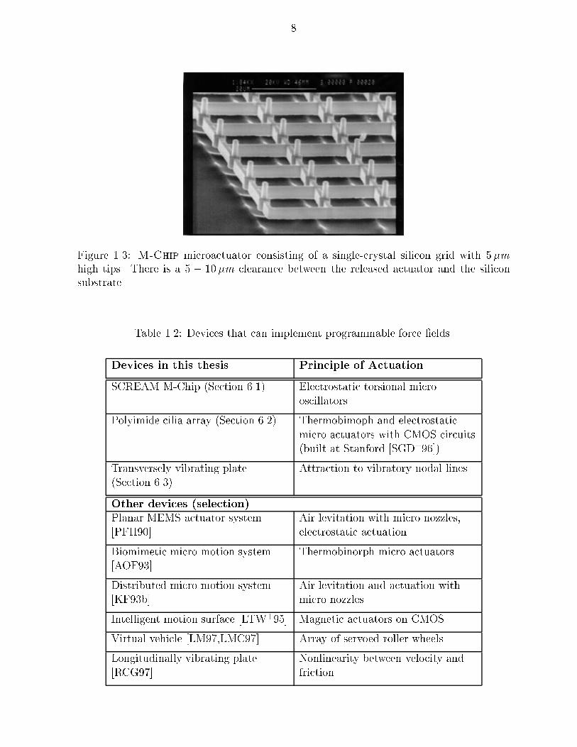
Figure 1.3: M-Chip microactuator consisting of a single-crystal silicon grid with 5�mhigh tips. There is a 5 � 10�m clearance between the released actuator and the siliconsubstrate.

Table 1.2: Devices that can implement programmable force �elds.

Devices in this thesis Principle of Actuation

SCREAM M-Chip (Section 6.1) Electrostatic torsional microoscillators

Polyimide cilia array (Section 6.2) Thermobimoph and electrostaticmicro actuators with CMOS circuits(built at Stanford [SGD+96])

Transversely vibrating plate(Section 6.3)

Attraction to vibratory nodal lines

Other devices (selection)Planar MEMS actuator system[PFH90]

Air levitation with micro nozzles,electrostatic actuation

Biomimetic micro motion system[AOF93]

Thermobinorph micro actuators

Distributed micro motion system[KF93b]

Air levitation and actuation withmicro nozzles

Intelligent motion surface [LTW+95] Magnetic actuators on CMOS

Virtual vehicle [LM97,LMC97] Array of servoed roller wheels

Longitudinally vibrating plate[RCG97]

Nonlinearity between velocity andfriction

9

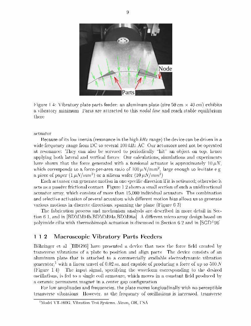
Parts

Node

Figure 1.4: Vibratory plate parts feeder: an aluminum plate (size 50 cm � 40 cm) exhibitsa vibratory minimum. Parts are attracted to this nodal line and reach stable equilibriumthere.

actuator.Because of its low inertia (resonance in the high kHz range) the device can be driven in a

wide frequency range from DC to several 100 kHz AC. Our actuators need not be operatedat resonance: They can also be servoed to periodically \hit" an object on top, henceapplying both lateral and vertical forces. Our calculations, simulations and experimentshave shown that the force generated with a torsional actuator is approximately 10�N ,which corresponds to a force-per-area ratio of 100�N=mm2, large enough to levitate e.g.a piece of paper (1�N=mm2) or a silicon wafer (10�N=mm2).

Each actuator can generate motion in one speci�c direction if it is activated; otherwise itacts as a passive frictional contact. Figure 1.2 shows a small section of such a unidirectionalactuator array, which consists of more than 15,000 individual actuators. The combinationand selective activation of several actuators with di�erent motion bias allows us to generatevarious motions in discrete directions, spanning the plane (Figure 6.3).

The fabrication process and mechanism analysis are described in more detail in Sec-tion 6.1, and in [BDMM94b,BDMM94a,BDM96a]. A di�erent micro array design based onpolyimide cilia with thermobimoph actuation is discussed in Section 6.2 and in [SGD+96].

1.1.2 Macroscopic Vibratory Parts Feeders

B�ohringer et al. [BBG95] have presented a device that uses the force �eld created bytransverse vibrations of a plate to position and align parts. The device consists of analuminum plate that is attached to a commercially available electrodynamic vibrationgenerator,1 with a linear travel of 0:02m, and capable of producing a force of up to 500N(Figure 1.4). The input signal, specifying the waveform corresponding to the desiredoscillations, is fed to a single coil armature, which moves in a constant �eld produced bya ceramic permanent magnet in a center gap con�guration.

For low amplitudes and frequencies, the plate moves longitudinally with no perceptibletransverse vibrations. However, as the frequency of oscillations is increased, transverse

1Model VT-100G, Vibration Test Systems, Akron, OH, USA.

10

vibrations of the plate become more pronounced. The resulting motion is similar to theforced transverse vibration of a rectangular plate, clamped on one edge and free alongthe other three sides. This vibratory motion creates a force �eld in which particles areattracted to locations with minimal vibration, called the nodal lines. This �eld can beprogrammed by changing the frequency, or by employing clamps as programmable �xturesthat create various vibratory nodes.

Figure 1.4 shows two parts, shaped like a triangle and a trapezoid, after they havereached their stable poses. To better illustrate the orienting e�ect, the curve showingthe nodal line has been drawn by hand. Nota bene: This device can only use the �nitemanipulation grammar described in Section 5.2 since it can only generate a constrainedset of vibratory patterns, and cannot implement general squeeze and radial strategies.

Section 6.3 gives more details on our manipulation experiments with transversely vi-brating plates.

Chapter 2

Equilibrium Analysis For

Programmable Vector Fields

For the generation of manipulation strategies with programmable vector �elds it is essentialto be able to predict the motion of a part in the �eld. Particularly important is determiningthe stable equilibrium poses a part can reach in which all forces and moments are balanced.This equilibrium analysis was introduced in our short conference paper [BDMM94a], wherewe presented a theory of manipulation for programmable vector �elds, and an algorithmthat generates manipulation strategies to orient polygonal parts without sensor feedbackusing a sequence of squeeze �elds. We now review the algorithm in [BDMM94a] andgive a detailed proof of its complexity bounds. The tools developed here are essential tounderstanding our new and improved results, and will be used throughout this thesis todevelop complexity bounds for our distributed manipulation algorithms.

We will in general assume that the dynamics of a part moving in the force �eld isgoverned by �rst-order dynamics. This assumption is based on extensive experimentationwith the devices presented in Section 6. In a �rst-order system, the velocity of a partis directly proportional to the force acting on it. Basically, it is a rigid body dynamicalsystem that is heavily damped.

2.1 Squeeze Fields and Equilibria

In [BDMM94a] we proposed a family of control strategies called squeeze �elds and a plan-ning algorithm for parts-orientation.

De�nition 1 [BDM96b] Assume l is a straight line through the origin. A squeeze �eldf is a two-dimensional force vector �eld de�ned as follows:

1. If z 2 R 2 lies on l then f(z) = 0.2. If z does not lie on l then f(z) is the unit vector normal to l and pointing towardsl.

We refer to the line l as the squeeze line, because l lies in the center of the squeeze�eld. See Figure 2.1 for examples of squeeze �elds.

Assuming quasi-static motion, an object will move perpendicularly towards the line land come to rest there. We are interested in the motion of an arbitrarily shaped (notnecessarily small) part P . Let us call P1, P2 the regions of P that lie to the left and to the

11

12

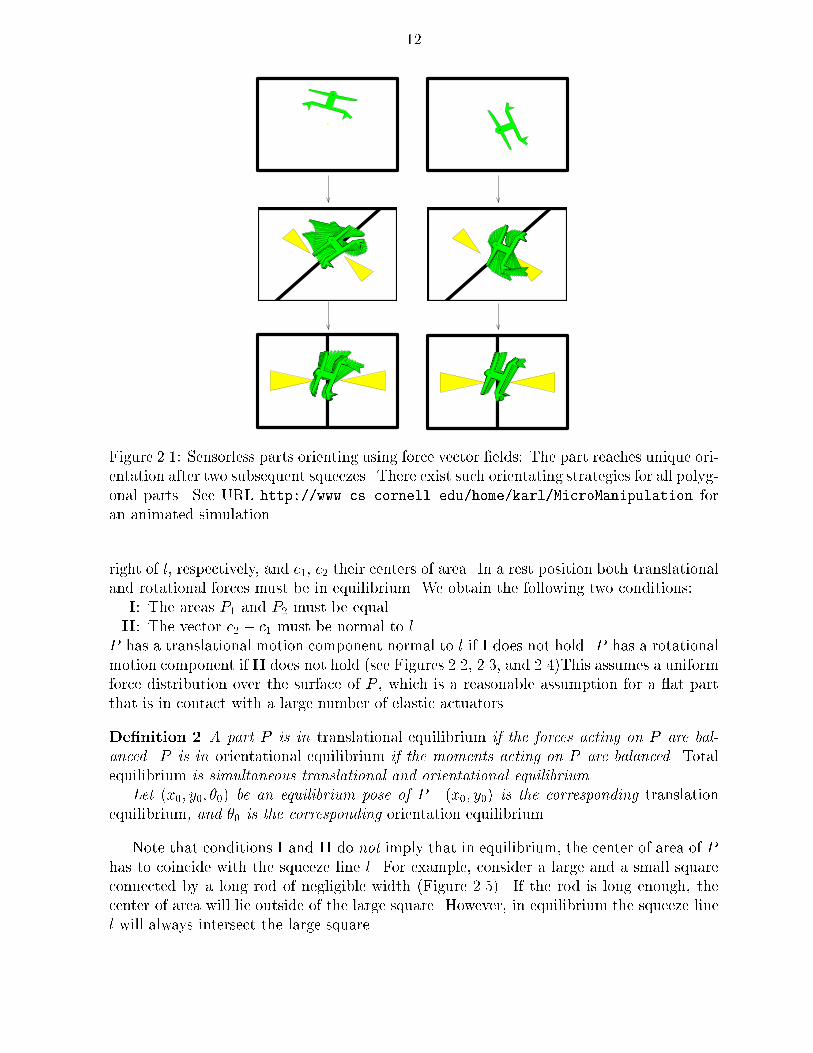
Figure 2.1: Sensorless parts orienting using force vector �elds: The part reaches unique ori-entation after two subsequent squeezes. There exist such orientating strategies for all polyg-onal parts. See URL http://www.cs.cornell.edu/home/karl/MicroManipulation foran animated simulation.

right of l, respectively, and c1, c2 their centers of area. In a rest position both translationaland rotational forces must be in equilibrium. We obtain the following two conditions:

I: The areas P1 and P2 must be equal.II: The vector c2 � c1 must be normal to l.

P has a translational motion component normal to l if I does not hold. P has a rotationalmotion component if II does not hold (see Figures 2.2, 2.3, and 2.4)This assumes a uniformforce distribution over the surface of P , which is a reasonable assumption for a at partthat is in contact with a large number of elastic actuators.

De�nition 2 A part P is in translational equilibrium if the forces acting on P are bal-anced. P is in orientational equilibrium if the moments acting on P are balanced. Totalequilibrium is simultaneous translational and orientational equilibrium.

Let (x0; y0; �0) be an equilibrium pose of P . (x0; y0) is the corresponding translationequilibrium, and �0 is the corresponding orientation equilibrium.

Note that conditions I and II do not imply that in equilibrium, the center of area of Phas to coincide with the squeeze line l. For example, consider a large and a small squareconnected by a long rod of negligible width (Figure 2.5). If the rod is long enough, thecenter of area will lie outside of the large square. However, in equilibrium the squeeze linel will always intersect the large square.

13

P1

P2

c1

squeeze line

c2

l

Figure 2.2: Equilibrium condition: To balance force and moment acting on P in a unitsqueeze �eld, the two areas P1 and P2 must be equal (i.e., l must be a bisector), and theline connecting the centers of area c1 and c2 must be perpendicular to the node line.

2.2 Polygon Bisectors and Complexity

Consider a polygonal part P in a unit squeeze �eld as described in Section 2.1. In thissection we describe how to determine the orientations �i in which P achieves equilibrium.This construction will show that equilibria always exist as long as the contact areas have�nite size, and that for connected parts the orientation equilibria are discrete. More pre-cisely, if a connected part is in equilibrium in a squeeze �eld, there are discrete values for itsorientation, and its o�set from the center of the squeeze line. The equilibrium is of courseindependent of its position along the squeeze line. Hence, in the remainder of Section 2,when using the term discrete equilibria, we mean that the orientation and o�set of the partis discrete. We will derive upper bounds on the number of these discrete equilibria.

De�nition 3 A bisector of a polygon P is a line that cuts P into two regions of equalarea.

Proposition 4 [BDM96b] Let P be a polygon whose interior is connected. There existO(k n2) bisectors such that P is in equilibrium when placed in a squeeze �eld such that thebisector coincides with the squeeze line. n is the part complexity measured as the numberof polygon vertices. k denotes the maximum number of polygon edges that a bisector cancross.

If P is convex, then the number of bisectors is bounded by O(n).

For most part geometries, k is a small constant.1 However in the worst-case, patholog-ical parts can reach k = O(n). A (e.g. rectilinear) spiral-shaped part would be an examplefor such a pathological case, because every bisector intersects O(n) polygon edges.

Lemma 5 Given a polygon P and a line l : y = mx + c. Let n be the number of verticesof P .

1In particular, in [BDMM94a] we assumed that k = O(1).

14

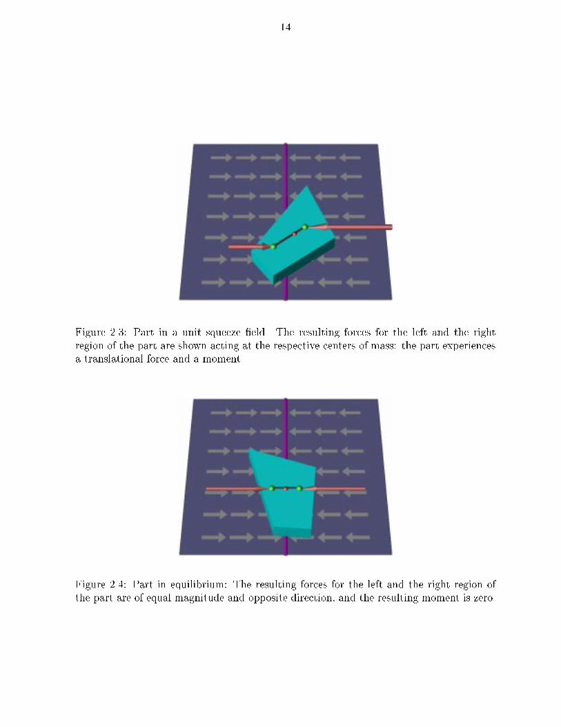
Figure 2.3: Part in a unit squeeze �eld. The resulting forces for the left and the rightregion of the part are shown acting at the respective centers of mass: the part experiencesa translational force and a moment.

Figure 2.4: Part in equilibrium: The resulting forces for the left and the right region ofthe part are of equal magnitude and opposite direction, and the resulting moment is zero.

15

COM

l

Figure 2.5: Part consisting of two squares connected by a long, thin rod. The part is intotal equilibrium, but its COM does not coincide with the squeeze line l.

1. There exist O(n2) combinatorially di�erent ways how a line l can intersect P .2. Let a and b be the intersections of bisector l with the convex hull of P . As m variesfrom �1 to +1, a and b progress monotonically counterclockwise about the convexhull of P .3. If the interior of P is connected, then there exists a unique bisector of P for everym 2 R .

Combinatorially equivalent intersections of polygon P are all those placements of theintersecting line l such that the sets of left and right polygon vertices are �xed. A necessarycondition for combinatorial equivalence is that l intersects the same ordered set of polygonedges.Proof:

1. There are O(n2) di�erent placements for l such that it coincides with more thanone vertex of P . Hence all placements of l fall into one of O(n2) combinatoriallyequivalent classes.

2. See [DO90, Lemma 3.1].3. Assume l is a bisector of P with a �xed slopem. Since P is connected, the intersection

between l and P must be a line segment of non-zero length. Hence a translation of le.g. towards the left will cause a strictly monotonous decrease of the left area segmentof P , and vice versa. Therefore the bisector placement of l for a given slope m isunique.

2

Consider the bisector l of polygon P for changing m values, as described in Lemma 5.The intersections of l with the convex hull of P , a and b, progress monotonically about theconvex hull. In general, this progression corresponds to a rotation and a translation of l.

In the following proof for Proposition 4, we investigate the relationship between thelocation of the bisector, and the corresponding left and right areas of P and its respectivecenters of mass. This will allow us to show that for combinatorially equivalent bisectorplacements there are only a �nite number of possible equilibria, and that this number isbounded by O(k).Proof: [Proposition 4] Consider two combinatorially equivalent placements of bisectorl on polygon P . We will show that the number of equilibria for this bisector placement isbounded by O(k). Since there are O(n2) such placements for P (see Lemma 5), the totalnumber of equilibria will be O(k n2).

16

s

r1

r02

r2a2

a1

l0 l

r

P

r0

r01

Figure 2.6: Two non-parallel lines l and l0 in combinatorially equivalent intersection withpolygon P .

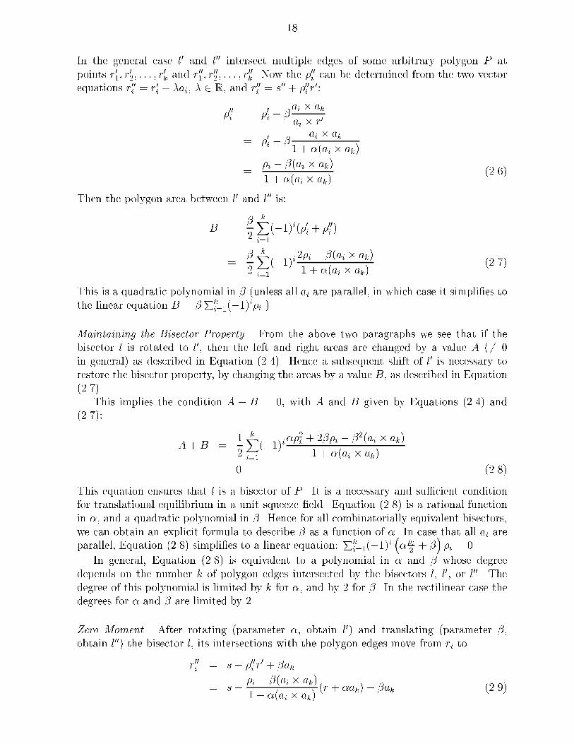
Rotating the Bisector. Consider the line l and a point s that lies on l (Figure 2.6). Thedirection of l is given by a vector r. Assume for now that the line l intersects two edgesof the polygon P in the points r1 and r2. Also assume that these edges have directions a1and a2. Now consider another line l0 with direction r0 that intersects l in s. Assume that land l0 have combinatorially equivalent intersections with polygon P , and that l0 intersectsthe polygon edges in r01 and r02. Let us write ri = s + �ir and r0i = s + �0ir

0. Then thepolygon area between l and l0 is:

A =1

2(�02r

0 � �2r � �01r0 � �1r)

=1

2(�02�2 � �01�1)(r

0 � r)

In the general case where l and l0 intersect multiple edges of some arbitrary polygon P atpoints r1; r2; : : : ; rk and r01; r

02; : : : ; r

0k (k even), the polygon area between l and l0 is:

A =1

2

kXi=1

(�1)iAi

=1

2(r0 � r)

kXi=1

(�1)i�0i�i

W.l.o.g. let �k 6= 0. Then r0 can be written as r0 = r+�ak for some � 2 R , and the aboveequation becomes:

=1

2((r + �ak)� r)

kXi=1

(�1)i�0i�i

=�

2(ak � r)

kXi=1

(�1)i�0i�i (2.1)

17

l0

P

a2

r002

l00

a1

r0

r001

r01

r02

s0 s00

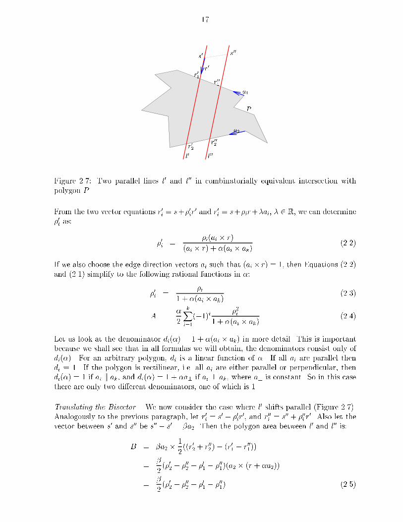
Figure 2.7: Two parallel lines l0 and l00 in combinatorially equivalent intersection withpolygon P .

From the two vector equations r0i = s+�0ir0 and r0i = s+�ir+�ai, � 2 R , we can determine

�0i as:

�0i =�i(ai � r)

(ai � r) + �(ai � ak)(2.2)

If we also choose the edge direction vectors ai such that (ai� r) = 1, then Equations (2.2)and (2.1) simplify to the following rational functions in �:

�0i =�i

1 + �(ai � ak)(2.3)

A =�

2

kXi=1

(�1)i �2i1 + �(ai � ak)

(2.4)

Let us look at the denominator di(�) = 1 + �(ai � ak) in more detail. This is importantbecause we shall see that in all formulas we will obtain, the denominators consist only ofdi(�). For an arbitrary polygon, di is a linear function of �. If all ai are parallel thendi = 1. If the polygon is rectilinear, i.e. all ai are either parallel or perpendicular, thendi(�) = 1 if ai k ak, and di(�) = 1 + �a? if ai ? ak, where a? is constant. So in this casethere are only two di�erent denominators, one of which is 1.

Translating the Bisector. We now consider the case where l0 shifts parallel (Figure 2.7).Analogously to the previous paragraph, let r0i = s0 + �0ir

0, and r00i = s00 + �00i r0. Also let the

vector between s0 and s00 be s00 � s0 = �a2. Then the polygon area between l0 and l00 is:

B = �a2 � 1

2((r02 + r002)� (r01 + r001))

=�

2(�02 + �002 � �01 � �001)(a2 � (r + �a2))

=�

2(�02 + �002 � �01 � �001) (2.5)

18

In the general case l0 and l00 intersect multiple edges of some arbitrary polygon P atpoints r01; r

02; : : : ; r

0k and r001 ; r

002 ; : : : ; r

00k. Now the �00i can be determined from the two vector

equations r00i = r0i + �ai, � 2 R , and r00i = s00 + �00i r0:

�00i = �0i � �ai � akai � r0

= �0i � �ai � ak

1 + �(ai � ak)

=�i � �(ai � ak)

1 + �(ai � ak)(2.6)

Then the polygon area between l0 and l00 is:

B =�

2

kXi=1

(�1)i(�0i + �00i )

=�

2

kXi=1

(�1)i2�i � �(ai � ak)

1 + �(ai � ak)(2.7)

This is a quadratic polynomial in � (unless all ai are parallel, in which case it simpli�es tothe linear equation B = �

Pki=1(�1)i�i ).

Maintaining the Bisector Property. From the above two paragraphs we see that if thebisector l is rotated to l0, then the left and right areas are changed by a value A (6= 0in general) as described in Equation (2.4). Hence a subsequent shift of l0 is necessary torestore the bisector property, by changing the areas by a value B, as described in Equation(2.7).

This implies the condition A + B = 0, with A and B given by Equations (2.4) and(2.7):

A+B =1

2

kXi=1

(�1)i��2i + 2��i � �2(ai � ak)

1 + �(ai � ak)

= 0 (2.8)

This equation ensures that l is a bisector of P . It is a necessary and su�cient conditionfor translational equilibrium in a unit squeeze �eld. Equation (2.8) is a rational functionin �, and a quadratic polynomial in �. Hence for all combinatorially equivalent bisectors,we can obtain an explicit formula to describe � as a function of �. In case that all ai areparallel, Equation (2.8) simpli�es to a linear equation:

Pki=1(�1)i

�� �i

2+ �

��i = 0.

In general, Equation (2.8) is equivalent to a polynomial in � and � whose degreedepends on the number k of polygon edges intersected by the bisectors l, l0, or l00. Thedegree of this polynomial is limited by k for �, and by 2 for �. In the rectilinear case thedegrees for � and � are limited by 2.

Zero Moment. After rotating (parameter �, obtain l0) and translating (parameter �,obtain l00) the bisector l, its intersections with the polygon edges move from ri to

r00i = s+ �00i r0 + �ak

= s+�i � �(ai � ak)

1 + �(ai � ak)(r + �ak) + �ak (2.9)

19

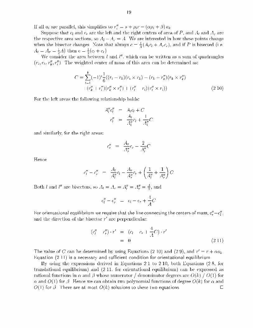
If all ai are parallel, this simpli�es to r00i = s+ �ir + (��i + �) ak.Suppose that cl and cr are the left and the right centers of area of P , and Al and Ar are

the respective area sections, so Al+Ar = A. We are interested in how these points changewhen the bisector changes. Note that always c = 1

A(Alcl +Arcr), and if P is bisected (i.e.

Al = Ar =12A) then c = 1

2(cl + cr).

We consider the area between l and l00, which can be written as a sum of quadrangles(ri; rk; r

00k; r

00i ). The weighted center of mass of this area can be determined as:

C =kX

i=1

(�1)i16((ri + rk)(ri � rk) + (rk + r00k)(rk � r00k)

+(r00k + r00i )(r00k � r00i ) + (r00i + ri)(r

00i � ri)) (2.10)

For the left areas the following relationship holds:

A00l c

00l = Alcl + C

c00l =Al

A00l

cl +1

A00l

C

and similarly, for the right areas:

c00r =Ar

A00r

cr � 2

A00l

C

Hence

c00l � c00r =Al

A00l

cl � Ar

A00r

cr +

1

A00l

+1

A00r

!C

Both l and l00 are bisectors, so Al = Ar = A00l = A00

r =A2, and

c00l � c00r = cl � cr +4

AC

For orientational equilibrium we require that the line connecting the centers of mass, c00r�c00l ,and the direction of the bisector r0 are perpendicular:

(c00l � c00r) � r0 = (cl � cr +4

AC) � r0

= 0 (2.11)

The value of C can be determined by using Equations (2.10) and (2.9), and r0 = r + �ak.Equation (2.11) is a necessary and su�cient condition for orientational equilibrium.

By using the expressions derived in Equations 2.1 to 2.10, both Equations (2.8, fortranslational equilibrium) and (2.11, for orientational equilibrium) can be expressed asrational functions in � and � whose numerator / denominator degrees are O(k) = O(1) for� and O(1) for �. Hence we can obtain two polynomial functions of degree O(k) for � andO(1) for �. There are at most O(k) solutions to these two equations. 2

20

2.3 Planning of Manipulation Strategies

In this section we present an algorithm for sensorless parts alignment with squeeze�elds [BDMM94a,BDM96b]. Recall from Section 2.2 that in squeeze �elds, the equilibriafor connected polygons are discrete (modulo a neutrally stable translation parallel to thesqueeze line which we will disregard for the remainder of Section 2).

To model our actuator arrays and vibratory devices, we made the following assump-tions:Density: The generated forces can be described by a vector �eld, i.e., the individual mi-

croactuators are dense compared to the size of the moving part.2Phase: The motion of a part has two phases: (1) Pure translation towards l until the

part is in translational equilibrium. (2) Motion in translational equilibrium untilorientational equilibrium is reached.

Note that due to the elasticity and oscillation of the actuator surfaces, we can assumecontinuous area contact, and not just contact in three or a few points. If a part moveswhile in translational equilibrium, in general the motion is not a pure rotation, but alsohas a translational component.

De�nition 6 [BDM96b] Let � be the orientation of a connected polygon P in a squeeze�eld, and let us assume that condition I holds. The turn function t : � ! f�1; 0; 1gdescribes the instantaneous rotational motion of P :

t(�) =

8><>:1 if P will turn counterclockwise

�1 if P will turn clockwise0 if P is in total equilibrium (Fig. 2.8).

See Figure 2.8 for an illustration. The turn function t(�) can be obtained e.g. by takingthe sign of the lifted moment MP (z) for poses z = (x; y; �) in which the lifted force fP (z)is zero.

De�nition 6 immediately implies the following lemma:

Lemma 7 [BDM96b] Let P be a polygon with orientation � in a squeeze �eld such thatcondition I holds. P is stable if t(�) = 0, t(�+) � 0, and t(��) � 0. Otherwise P isunstable.

Proof: Assume the part P is in a pose (x; y; �) such that condition I is satis�ed. Thisimplies that the translational forces acting on P balance out. If in addition t(�) = 0,then the e�ective moment is zero, and P is in total equilibrium. Now consider a smallperturbation �� > 0 of the orientation � of P while condition I is still satis�ed. For a stableequilibrium, the moment resulting from the perturbation �� must not aggravate but rathercounteract the perturbation. This is true if and only if t(� + ��) � 0 and t(� � ��) � 0. 2

Using this lemma we can identify all stable orientations, which allows us to construct thesqueeze function [Gol93] of P (see Figure 2.8c), i.e. the mapping from an initial orientationof P to the stable equilibrium orientation that it will reach in the squeeze �eld:

Lemma 8 [BDM96b] Let P be a polygonal part on an actuator array A such that as-sumptions Density and 2Phase hold. Given the turn function t of P , its correspondingsqueeze function s : S1 ! S

1 is constructed as follows:1. All stable equilibrium orientations � map identically to �.

21

s

t

π 2π

2ππ(b)

(c) (d)

(a)

π

2π

Figure 2.8: (a) Polygonal part. Stable (thick line) and unstable (thin line) bisectors arealso shown. (b) Turn function, which predicts the orientations of the stable and unstablebisectors. (c) Squeeze function, constructed from the turn function. (d) Alignment strat-egy for two arbitrary initial con�gurations. See URL http://www.cs.cornell.edu/home

/karl/Cinema for an animated simulation.

2. All unstable equilibrium orientations map (by convention) to the nearest counter-clockwise stable orientation.3. All orientations � with t(�) = 1 (�1) map to the nearest counterclockwise (clock-wise) stable orientation.

Then s describes the orientation transition of P induced by A.Proof: Assume that part P initially is in pose (x; y; �) in array A. Because of 2Phase,we can assume that P translates towards the center line l until condition I is satis�edwithout changing its orientation �. P will change its orientation until the moment is zero,i.e. t = 0: A positive moment (t > 0) causes counterclockwise motion, and a negativemoment (t < 0) causes clockwise motion until the next root of t is reached. 2

We conclude that any connected polygonal part, when put in a squeeze �eld, reachesone of a �nite number of possible orientation equilibria [BDMM94a,BDM96b]. The motionof the part and, in particular, the mapping between initial orientation and equilibriumorientation is described by the squeeze function, which is derived from the turn functionas described in Lemma 8. Note that all squeeze functions derived from turn functions aremonotone step-shaped functions.

Goldberg [Gol93] has given an algorithm that automatically synthesizes a manipulationstrategy to uniquely orient a part, given its squeeze function. While Goldberg's algorithmwas designed for squeezes with a robotic parallel-jaw gripper, in fact, it is more general,and can be used for arbitrary monotone step-shaped squeeze functions. The output ofGoldberg's algorithm is a sequence of angles that specify the required directions of thesqueezes. Hence these angles specify the direction of the squeeze line in our force vector

22

unstable

stable unstable

(a) Parallel-Jaw Gripper

stable

(b) Squeeze Field

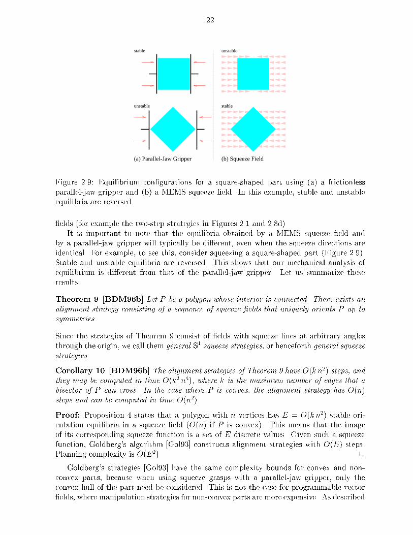
Figure 2.9: Equilibrium con�gurations for a square-shaped part using (a) a frictionlessparallel-jaw gripper and (b) a MEMS squeeze �eld. In this example, stable and unstableequilibria are reversed.

�elds (for example the two-step strategies in Figures 2.1 and 2.8d).It is important to note that the equilibria obtained by a MEMS squeeze �eld and

by a parallel-jaw gripper will typically be di�erent, even when the squeeze directions areidentical. For example, to see this, consider squeezing a square-shaped part (Figure 2.9).Stable and unstable equilibria are reversed. This shows that our mechanical analysis ofequilibrium is di�erent from that of the parallel-jaw gripper. Let us summarize theseresults:

Theorem 9 [BDM96b] Let P be a polygon whose interior is connected. There exists analignment strategy consisting of a sequence of squeeze �elds that uniquely orients P up tosymmetries.

Since the strategies of Theorem 9 consist of �elds with squeeze lines at arbitrary anglesthrough the origin, we call them general S1 squeeze strategies, or henceforth general squeezestrategies.

Corollary 10 [BDM96b] The alignment strategies of Theorem 9 have O(k n2) steps, andthey may be computed in time O(k2 n4), where k is the maximum number of edges that abisector of P can cross. In the case where P is convex, the alignment strategy has O(n)steps and can be computed in time O(n2).

Proof: Proposition 4 states that a polygon with n vertices has E = O(k n2) stable ori-entation equilibria in a squeeze �eld (O(n) if P is convex). This means that the imageof its corresponding squeeze function is a set of E discrete values. Given such a squeezefunction, Goldberg's algorithm [Gol93] constructs alignment strategies with O(E) steps.Planning complexity is O(E2). 2

Goldberg's strategies [Gol93] have the same complexity bounds for convex and non-convex parts, because when using squeeze grasps with a parallel-jaw gripper, only theconvex hull of the part need be considered. This is not the case for programmable vector�elds, where manipulation strategies for non-convex parts are more expensive. As described

23

a10 a20 a30

R10 R20 R30 b

Figure 2.10: Sample rectangles R10, R20, and R30. Edge a is 10, 20, and 30% longer thanedge b, respectively.

in Section 2.2, there could exist parts that have E = (k n2) orientation equilibria ina squeeze �eld, which would imply alignment strategies of length (k n2) and planningcomplexity (k2 n4).

Note that the turn and squeeze functions have a period of � due to the symmetry ofthe squeeze �eld; rotating the �eld by an angle of � produces an identical vector �eld.Rotational symmetry in the part also introduces periodicity into these functions. Hence,general squeeze strategies (see Theorem 9) orient a part up to symmetry, that is, up tosymmetry in the part and in the squeeze �eld. Similarly, the grasp plans based on squeezefunctions in [Gol93] can orient a part with a macroscopic gripper only modulo symmetry inthe part and in the gripper.2 Since we reduce to the squeeze function algorithm in [Gol93],it is not surprising that this phenomenon is also manifested for squeeze vector �elds aswell. For a detailed discussion of parts orientation modulo symmetry see [Gol93].

In Section 5.1 we will present new and improved manipulation algorithms that reducethe number of equilibria to E = O(k n).

This scheme may be generalized to the case where l is slightly curved, as in the \node"of the vibrating plate in Figure 1.4. See [BBG95] for details. The remaining sections ofthis paper investigate using more exotic �elds (not simple squeeze patterns) to

1. allow disconnected polygons,2. relax assumption 2Phase,3. reduce the planning complexity,4. reduce the number of equilibria,5. reduce the execution complexity (strategy length), and6. determine feasibility results and limitations for manipulation with general force �elds.

2.4 Example: Uniquely Orienting Rectangular Parts

To demonstrate the equilibrium analysis from Section 2.1 and the alignment algorithmfrom Section 2.3, we will generate plans for uniquely orienting several planar polygonalparts (up to part symmetry). In particular, here we will consider the simple case of threerectangles R10, R20, and R30, which have sides a and b such that a is 10, 20, and 30 percentlonger than b, respectively (Figure 2.10).

Our algorithm �rst determines stable and unstable equilibria of the parts, which corre-spond to the negative and positive steps in the turn function, respectively (see Lemma 7).

2Parallel-jaw gripper symmetry is also modulo �.

24

l

a=2

R

c1

c2

x

y

(a=2; �)

b=2

c0

�

Figure 2.11: Analytically determining the moment function for a rectangular part R withsides of length a and b. c0 is the center of mass of the segment below the x-axis. c1 and c2are the centers of the triangular segments between x-axis and line l.

Table 2.1: Equilibria of rectangular parts R10, R20, and R30 in a unit squeeze �eld withvertical squeeze line.

Part Equilibrium orientations �stable unstable

R10 0:97; 2:18; 4:11; 5:32 0; �=2; �; 3�=2R20 1:29; 1:85; 4:43; 4:99 0; �=2; �; 3=pi=2R30 �=2; 3�=2 0; �

The turn function can be obtained as the sign of the moment function, which, for polyg-onal parts, is a piecewise rational function, and can be derived automatically from thepart geometry. For example, consider the rectangle R in Figure 2.11: A line l through theorigin bisects R. If l is placed such that it intersects the right edge of R at (a=2; �) with�b=2 � � � b=2, then the COM of the segment below l is

c� =

ab

2c0 +

a�

4(c1 � c2)

!2

ab

= c0 +�

2b2c1

= (a�

3b;� b

4+�2

3b)

The moment function is the inner product between the vector c�, and the direction ofthe line l. For balanced moment, this product must be zero, which gives us the followingcondition for equilibrium:

0 = (a�

3b;� b

4+�2

3b) � (a

2; �)

=a2�

6b� b�

4+�3

3b

25

−6 −4 −2 0 2 4 6−5

−4

−3

−2

−1

0

1

2

3

4

5

(a) −6 −4 −2 0 2 4 6−5

−4

−3

−2

−1

0

1

2

3

4

5

(b)

−6 −4 −2 0 2 4 6−5

−4

−3

−2

−1

0

1

2

3

4

5

(c)

Figure 2.12: Stable (dark) and unstable (white) equilibria of three rectangular parts in aunit squeeze �eld with vertical squeeze line: (a) R10, edge ratio 1.1; (b) R20, edge ratio 1.2;(c) R30, edge ratio 1.3. R10 and R20 exhibit two stable equilibria, R30 exhibits only one.

=�

12b(2a2 � 3b2 + 4�2)

So � = 0

or � = �1

2

p3b2 � 2a2

= � b

2

p3� 2c2 for a = cb

This means that for rectangles with edge ratio c �q3=2 � 1:22 (such as R10 and R20),

there exist equilibrium orientations at angles � = arctan(�q3=c2 � 2). For rectangles

with larger edge ratio c (such as R30), an equilibrium exists only at � = 0. A similaranalysis can be performed for all other placements of the line l, see [BDM96b] for moredetails. Equilibrium orientations as determined by our planner are shown in Figure 2.12and Table 2.1. Since all of our parts are symmetric with respect to rotation by �, for theremainder of this example we will consider all angles modulo �.

From the equilibrium orientations in Table 2.1 the algorithm generates the squeezefunction, according to Lemma 8. Note that steps in the squeeze function occur at anglescorresponding to unstable equilibria, while the image of the squeeze function is the set ofall stable equilibrium orientations (see Figure 2.13).

Finally, the squeeze function is used as input for Goldberg's planning algorithm [Gol93],which returns as output a sequence of squeeze angles. A sequence of two squeeze �elds, witha relative angle of �=2, is su�cient to uniquely orient both R10 and R20. See Figure 2.14for a sample execution of this plan for two arbitrary initial poses. R30 requires only onesqueeze �eld at an arbitrary angle.

It was shown in [BDM96b] that this algorithm can uniquely orient arbitrary polygons

26

0 1 2 3 4 5 6 7−0.06

−0.04

−0.02

0

0.02

0.04

0.06moment function

0 1 2 3 4 5 6 7

−1

−0.5

0

0.5

1

turn function

0 1 2 3 4 5 6 70

1

2

3

4

5

6squeeze function

(a)

0 1 2 3 4 5 6 7−0.1

−0.05

0

0.05

0.1moment function

0 1 2 3 4 5 6 7

−1

−0.5

0

0.5

1

turn function

0 1 2 3 4 5 6 70

1

2

3

4

5squeeze function

(b)

0 1 2 3 4 5 6 7−0.15

−0.1

−0.05

0

0.05

0.1

0.15moment function

0 1 2 3 4 5 6 7

−1

−0.5

0

0.5

1

turn function

0 1 2 3 4 5 6 70

1

2

3

4

5squeeze function

(c)

Figure 2.13: Moment function, turn function, and squeeze function for three rectangularparts: (a) R10, edge ratio 1.1; (b) R20, edge ratio 1.2; (c) R30, edge ratio 1.3. R10 and R20

exhibit two stable equilibria for � in the range [0 : : : �], R30 exhibits only one.

27

Step 1

# #

Step 2

Figure 2.14: Two-step alignment plan for rectangle R20. After two steps, R20 reaches aunique orientation � independent of its initial pose. However, the position (x; y) is notunique.

from any initial con�guration (up to part symmetry). However, recall that for this al-gorithm to work we have made several important assumptions that idealize the practicalvibratory feeding devices presented in Section 6.3.

1. 2Phase assumption, which states that translational and rotational motion of thepart is decoupled, implying that the turn function is independent of the initial o�setof the part from the squeeze line; see also Section 2.5.

2. Depending on the part shape, the algorithm may generate alignment plans with unitsqueeze �elds at arbitrary angles. Due to mechanical design limitations, usually notall of these �elds will be feasible to implement on most vibratory device setups.

3. The resulting plans uniquely orient a part, but the �nal translational position cannot be predicted.

In the remainder of this thesis, we will investigate new manipulation strategies that ad-dress these key issues. In particular, in Section 5.2 we will develop algorithms for deviceswith a limited \vocabulary" of available force �elds, which will result in a \manipulationgrammar" for unique, sensorless posing strategies for arbitrary planar, polygonal parts.

2.5 Relaxing the 2Phase Assumption

In Section 2.3, assumption 2Phase allowed us to determine successive equilibrium po-sitions in a sequence of squeezes, by a quasi-static analysis that decouples translationaland rotational motion of the moving part. For any part, this obtains a unique orientationequilibrium (after several steps). If 2Phase is relaxed, we obtain a dynamic manipulationproblem, in which we must determine the equilibria (x; �) given by the part orientation �and the o�set x of its center of mass from the squeeze line. A stable equilibrium is a (xi; �i)

28

pair in R �S1 that acts as an attractor (the x o�set in an equilibrium is, surprisingly, usu-ally not 0, see Figure 2.5). Again, we can compute these (xi; �i) equilibrium pairs exactly,as outlined in Section 2.2.

Considering (xi; �i) equilibrium pairs has another advantage. We can show that, evenwithout 2Phase, after two successive, orthogonal squeezes, the set of stable poses of anypart can be reduced from C = R

2 � S1 to a �nite subset of C (the con�guration space

of part P ); see Claim 39 (Section 5.2.1). Subsequent squeezes will preserve the �nitenessof the state space. This will signi�cantly reduce the complexity of a task-level motionplanner. Hence if assumption 2Phase is relaxed, this idea still enables us to simplify thegeneral motion planning problem (as formulated e.g. by Lozano-P�erez, Mason, and Taylorin [LPMT84]) to that of Erdmann and Mason [EM88]. Conversely, relaxing assumption2Phase raises the complexity from the \linear" planning scheme of Goldberg [Gol93] tothe forward-chaining searches of Erdmann and Mason [EM88], or Donald [Don90].

Chapter 3

Lower Bounds: What Programmable

Vector Fields Cannot Do

We now present \lower bounds" | constituting vector �elds and parts with pathologicalbehavior, making them unusable for manipulation. These counterexamples show that wemust be careful in choosing programmable vector �elds, and that, a priori , it is not obviouswhen a �eld is well-behaved.

3.1 Unstable Fields

In Section 2 we saw that in a vector �eld with a simple squeeze pattern (see again Fig-ure 2.1), polygonal parts reach certain equilibrium poses. This raises the question of ageneral classi�cation of all those vector �elds in which every part has stable equilibria.There exist vector �elds that do not have this property even though they are very similarto a simple squeeze.

De�nition 11 A skewed �eld fS is a vector �eld given by fS(x; y) = �sign(x)(1; �), where0 6= � 2 R .Proposition 12 A skewed �eld induces no stable equilibrium on a disk-shaped part.

Proof: Consider Figure 3.1, which shows a skewed �eld with � = �23: Only when the

center of the disk coincides with the center of the squeeze pattern do the translationalforces acting on the disk balance. But it will still experience a positive moment that willcause rotation. 2

Proposition 13 A diagonally skewed �eld (� = �1) induces no stable equilibrium on asquare-shaped part.

Proof: To reach equilibrium in a diagonally skewed �eld, the squeeze line has to bisect thepart such that the connector between the left and the right centers of area is diagonal (i.e.,parallel to the force vectors). An analysis similar to the proof of Proposition 4 (Section 2.2)or Figure 2.11 (Section 2.4) shows that for a square, no bisector placement can achieve anangle with the connector of less than 83�. 2

29

30

Figure 3.1: Unstable part in the skewed squeeze �eld (� = �23). The disk with center on

the squeeze line will keep rotating. Moreover, it has no stable equilibrium in this �eld.

Figure 3.2: S-shaped part PS with four rigidly connected point-contact \feet" in unstabletotal equilibrium (forces and moments balance). There exists no stable equilibrium positionfor this part in a vector �eld with a simple squeeze pattern. For an animation see URLhttp://www.cs.cornell.edu/home/karl/MicroManipulation/Patho.

3.2 Unstable Parts

Similarly we would like to identify the class of all those parts that always reach stableequilibria in particular vector �elds. From Section 2 we know that connected polygons insimple squeeze �elds satisfy this condition. This property relies on �nite area contacts: itdoes not hold for point contacts. As a counterexample consider the part PS in Figure 3.2.Proposition 14 There exist parts that do not have stable equilibria in a simple squeeze�eld.

Proof: The S-shaped part in Figure 3.2 has four rigidly connected \feet" with smallcontact surfaces. As the area of each of these four feet approaches zero, the part has nostable equilibrium in a simple squeeze �eld. There is only one orientation for the part inwhich both force and moment balances out, and this orientation is unstable. 2

In Section 4.2 we will discuss this phenomenon in greater detail, after the tools necessaryfor a complete mathematical analysis have been developed.

Finally, the number of stable equilibria of a given part in uences both the planningcomplexity and the plan length of an alignment strategy. It also a�ects the resolution ofthe vector �eld that is necessary to perform a strategy accurately. Even though all parts wehave considered exhibit only one or two orientation equilibria, there exist no tight boundson the maximum number of orientation equilibria in a unit squeeze �eld.

31

Proposition 15 Let n be the number of vertices of a polygon P , and let k be the maximumnumber of edges that a bisector of P can cross:

A. Regular polygons have n stable orientation equilibria in a squeeze �eld.B. Every connected polygon has O(k n2) stable orientation equilibria in a squeeze �eld.

Proof:A. Because of their part symmetry, regular polygons have 2n equilibria. Half of them

are stable, the other n are unstable.B. See Section 2.2.

2

As described in Section 2.2, there exist simple polygons with n vertices that can bebisected by a straight line in up to O(k n2) topologically di�erent ways [BDH97]. Thissuggests that there could be parts that have (k n2) orientation equilibria in a squeeze�eld, which would imply alignment strategies of length (k n2) and planning complexity(k2 n4).

While the counterexample in Figure 3.2 may be plausibly avoided by prohibiting partswith \point contacts," the other examples (Figure 3.1 and Proposition 15B) are more prob-lematic. In Section 4, we show how to choose programmable vector �elds that exclude someof these pathological behaviors, by using the theory of potential �elds to describe a class offorce vector �elds for which all polygonal parts have stable equilibria. In Section 5.1, weshow how to combine these �elds to obtain new �elds in which all parts have only O(k n)equilibria.

We believe parts with point contact (not having �nite area contact) will behave badlyin all vector �elds. We can model a point contact with delta functions, such that e.g. for

a point contact P0 at (x0; y0):ZP0

f dA =Zf �(x0; y0) dA = f(x0; y0). This model is

frequently used in mechanics (see e.g. [Erd94]). Point contact permits rapid, discontinuouschanges in force and moment. Hence, bodies with point contact will tend to exhibitinstabilities, as opposed to at parts that are in contact with a large number of (elastic)actuators. Finally, we believe that as the area contact|the size of the \feet" of a part|approaches zero, the part may become unstable. This represents a design constraint onparts which are to be manipulated using programmable planar parts feeders.

The lower bounds we demonstrate are indications of the pathologies that can arisewhen �elds without potential or parts with point contact are permitted. Each of ourcounterexamples (Figures 3.1 and 3.2) is \generic" in that it can be generalized to a verylarge class of similar examples. However, these lower bounds are just a �rst step, and onewishes for examples that delineate the capabilities of programmable vector �elds for planarparts manipulation even more precisely.

The separating �eld shown in Figure 1.1c is not a potential �eld, and there exist partsthat will spin forever, without equilibrium, in this �eld (this follows by generalizing theconstruction in Figure 3.1). However, for speci�c parts, such as those shown in Figure 1.1,this �eld is useful if we can pose the parts appropriately �rst (e.g., using the potential �eldshown in Figure 1.1b).

Finally, we may \surround" non-potential �elds with potential �elds to obtain reason-able behavior in some cases. Figure 1.1 shows how to \surround" a non-potential �eld intime by potential �elds, to eliminate pathologies. Similarly, we can surround non-potential�elds spatially . For example, if �eld 1.1c could be surrounded by a larger potential �eld,then after separation, parts can reach a stable equilibrium.

32

Non-potential �elds can be used safely with the following methodology: Let H � C =R

2�S1 be the undesirable limit set. For example, H could be a limit cycle where the partspins forever. Let bPV (H) be the weak pre-image [LPMT84,Don89] of H under the �eld V .If we can ensure that the part starts in a con�guration z 62 bPV (H), it will not reach theunwanted limit cycle. For example, in Figure 1.1 the centering step (b) ensures that thepart does not end up on the border between the two separating �elds, where it would spinforever in step (c).

Chapter 4

Completeness: Classi�cation Using

Potential Fields

We are interested in a general classi�cation of all those vector �elds in which every parthas stable equilibria. As motivation, recall that a skewed vector �eld, even though verysimilar to a regular squeeze �eld (see again Figure 2.1), induces no stable equilibrium in adisk-shaped part (Figure 3.1). In this section we give a family of vector �elds that will beuseful for manipulation tasks. These �elds belong to a speci�c class of vector �elds: theclass of �elds that have a potential.

We believe that �elds without potential will often induce pathological behavior in manyparts. Fields without potential admit paths along which a particle (point mass) will gainenergy. Since mechanical parts are rigid aggregations of particles, this may induce unstablebehavior in larger bodies. However, there are some cases where non-potential �elds maybe useful. For example, see Figure 1.1c, which is not a potential �eld. Such �elds maybe employed to separate but not to stabilize, pose, or orient parts. This strong statementdevolves to our proof that �elds like Figure 3.1 do not have well-behaved equilibria. Hence,they should only be employed when we want to induce an unstable system that will castparts away from equilibrium, e.g. in order to sort or separate them.

Consider the class of vector �elds on R2 that have a potential, i.e. �elds f in which

the work is independent of the path, or equivalently, the work on any closed path is zero,If �ds = 0. In a potential �eld each point (x; y) is assigned a real value U(x; y) that can be

interpreted as its potential energy. When U is smooth, then the vector �eld f associatedwith U is the gradient �rU . In general, U(x; y) is given, up to an additive constant, by

the path integralZ�f � ds (when it exists and it is unique), where � is an arbitrary path

from a �xed reference point (x0; y0) to (x; y). Assuming �rst-order dynamics, When U issmooth, an ideal point object is in stable equilibrium when it is at a local minimum of U .

De�nition 16 Let f be a force vector �eld on R 2, and let p be a point that is o�set froma �xed reference point q by a vector r(p) = p � q. We de�ne the generalized force F asthe force and moment induced by f at point p:

F (p) = (f(p) ; r(p)� f(p)) (4.1)

Let P be a part of arbitrary shape, and let Pz denote the part P in pose z = (x; y; �) 2 C.

33

34

liftin

g: a

rea

inte

gral

potential: path integral

FP UP

Uf

ZP Z

�

Z� Z

P

Figure 4.1: Determining the potential, and lifting are commutative operations on forcevector �elds.

We de�ne the lifted force �eld fP as the area integral of the force induced by f over Pz:

fP (z) =ZPzf dA (4.2)

The lifted generalized force �eld FP is de�ned as the area integral of the force and momentinduced by f over P in con�guration z:

FP (z) =ZPzF dA

=�Z

Pzf dA ;

ZPzr� f dA

�(4.3)

Hence, FP is a vector �eld on C. Finally, we de�ne the lifted potential UP : C ! R . UP

is the area integral of the potential U over P in con�guration z:

UP (z) =ZPzU dA (4.4)

We now show that the category of potential �elds is closed under the operation of lifting,and that UP is the potential of FP (see Figure 4.1). Note that U need not be smooth.

Let g : X ! Y and h : Y ! Z. Let k : X ! Z be the function which is the compositionof g and h, de�ned by k(x) = h(g(x)). In the following proposition, we use the notationh(g) to denote k, the function composition of g and h.

Proposition 17 Let f be a force �eld on R2 with potential U , and let P be a part of

arbitrary shape. For the lifted generalized force �eld FP and the lifted potential UP the

following equality holds: UP =ZPU dA =

Z�FP � dz+ c, where � is an arbitrary path in C

from a �xed reference point, and c is a constant.

Proof: Given a force �eld f with potential U , and a part P . We de�ne P � as the setf(r; �) j (r cos �; r sin �) 2 Pg � R � S

1. P � is a representation of P in polar coordinates:p = (r cos �; r sin �) 2 P if and only if (r; �) 2 P �.

We write Pz to denote P in pose z = (xz; yz; �z). If P is moved into pose z, then thepoint p moves to pz = (xz+r cos(�z+�) ; yz+r sin(�z+�)) = (xz; yz)+rz. Let us assumethat for a given P , the COM of P is at 0; this implies that the COM of Pz lies at (xz; yz).

35

We de�ne three families of functions �, �, and � as follows:�r;� : [0; 1] ! R

2

such that �r;� is a smooth path in R 2 with �r;�(0) = 0 and �r;�(1) = p0 = (r cos �; r sin �).�z : [0; 1] ! R

2 � S1

such that �z is a smooth path in R 2 � S1 with �z(0) = 0 and �z(1) = z = (xz; yz; �z).

�r;� : R2 � S

1 ! R2

(x; y; �) 7! (x+ r cos(� + �) ;y + r sin(� + �))

So �z is an arbitrary smooth path from 0 to z in C, and �r;�(�z) is a smooth path inR

2 from p0 = (r cos �; r sin �) to pz = (xz + r cos(�z + �) ; yz + r sin(�z + �)). Recall that�r;�(�z) is the function composition of �z and �r;�.

We are interested in the potential of U at pz.

U(pz) =Z�f � ds

where � is some path from 0 to pz. The integral is path-independent because f has potential U . Since we can chooseany path, we choose a path � that consists of two parts: (1) apath from 0 to the point p0, and (2) a path from p0 to pz.

=Z�r;�

f � ds +Z�r;�(�z)

f � dsNote that the path �r;�(�z), given by the composition of �z and�r;�, depends on z as well as on r and �, but �r;� is independentof z. The left integral is the potential di�erence between p0 and0. W.l.o.g. let us choose U(0) = 0.

= U(p0) +Z�zf(�r;�) � (J dz)

where J is the Jacobian

J =

@�x@x

@�x@y

@�x@�

@�y@x

@�y@y

@�y@�

!=�1 0 �r sin(�+�)0 1 r cos(�+�)

�which is the derivative of �r;�. f(�r;�) is the function composi-tion of �r;� and f . Also note that dz = (dx; dy; d�).

= U(p0) +Z�z

�fx(�r;�) ; fy(�r;�) ;

r cos(� + �)fy(�r;�)� r sin(� + �)fx(�r;�)) � dz

= U(p0) +Z�zF (�r;�) � dz (4.5)

Equation 4.5 states that the potential at a point pz = (xz+r cos(�z+�) ; yz+r sin(�z+�)) can be determined as the sum of two integrals: The �rst integrates the force f overa path from 0 to p0 = (r cos �; r sin �). If we choose U(0) = 0, then the �rst integral isthe potential at point p0. The right part of the expression can be understood as the pathintegral of the generalized force from p0 to pz.

With this result, we can now consider the lifted potential UP at a point z =

36

(xz; yz; �z) 2 C.

UP (z) =ZPzU(p) dA

=ZZP �

U(pz) r dr d�

where pz = (xz + r cos(�z + �) ; yz + r sin(�z + �)) such that(r; �) 2 P �.

=ZZP �

�U(p0) +

Z�zF (�r;�) � dz

�r dr d�

by using Equation 4.5. Again, F (�r;�) denotes the function com-position of �r;� and F .

=ZZP �

U(p0) r dr d� +ZZP �

�Z�zF (�r;�) � dz

�r dr r�

The �rst expression is the area integral of U over P . FromDe�nition 16 it follows that this expression is equal to UP (0)(note that UP (0) is a constant which does not depend on z).

= UP (0) +ZZP �

�Z 1

0F (�r;�(�z(t))) � � 0z(t) dt

�r dr r�

where � 0z is the derivative of �z. The dot product yields a scalarvalue. We can now switch the integrals.

=Z 1

0

�ZZP �

F (�r;�(�z(t))) � � 0z(t) r dr d��dt+ UP (0)

� 0z is constant with respect to the integration parameters r and�. Hence we can move � 0z outside of the area integral.

=Z 1

0

�ZZP �

F (�r;�(�z(t))) r dr d��� � 0z(t) dt+ UP (0)

=Z 1

0

�ZZP �

F (�z;x(t) + r cos(�z;�(t) + �) ;

�z;y(t) + r sin(�z;�(t) + �)) r dr d��� � 0z(t) dt+ UP (0)

where �z = (�z;x ; �z;y ; �z;�).

=Z 1

0

ZZP �

�z(t)

F (r cos �; r sin �) r dr d�

!� � 0z(t) dt+ UP (0)

where P ��z(t)

= f(r; �) j (r cos �; r sin �) 2 P�z(t)g.

=Z 1

0

ZP�z(t)

F dA

!� � 0z(t) dt+ UP (0)

=Z 1

0FP (�z(t)) � � 0z(t) dt+ UP (0)

by de�nition of the lifted force FP .

=Z�zFP � dz+ UP (0)

Hence UP is indeed the potential of FP . 2

37

S

�

z

z0

Pz0

Pz

p0p

Figure 4.2: Two triangles Pz and Pz0 with reference points z and z0 whose symmetricdi�erence is less than �.

We believe that a shorter proof is possible by using di�erential forms for the case thatboth f and U are smooth. However, since the �elds in consideration are usually not smooth(e.g. unit squeeze or radial �elds) we give the longer general proof here.

Corollary 18 Let f be a force �eld on R 2 with potential U , and let P be a part of arbitraryshape. For the lifted generalized force FP and the lifted potential UP the following equalityholds if UP is di�erentiable: rUP = �FP .

Proof: Follows directly from Proposition 17. 2

So again, UP (x; y; �) can be interpreted as the potential energy of part P in con�g-uration (x; y; �). Therefore we obtain a lifted potential �eld UP whose local minima arethe stable equilibrium con�gurations in C for part P . Furthermore, potential �elds areclosed under addition and scaling. We can thus create and analyze more complex �elds bylooking at their components. In general, the theory of potential �elds allows us to classifymanipulation strategies with vector �elds, o�ering new insights into equilibrium analysisand providing the means to determine strategies with stable equilibria. For example, itallows us to show that orientation equilibrium in a simple squeeze �eld is equivalent to thestability of a homogeneous boat oating in water, provided its density is � = 1

2�water (for

references on boat stability see e.g. [Gil56, pp. 42�] or [New77, pp. 290�]).

4.1 Properties of Lifted Force and Potential Fields

In this section we show that for a polygonal part P , the lifted force �eld is always contin-uous, and the lifted potential is always smooth.

Proposition 19 Consider a polygon P at two con�gurations z = (x; y; �) and z0 =(x0; y0; �0), z; z0 2 C = R

2 � S1. For all � > 0 there exists a � > 0 such that if z0 lies

within a �-ball around z, z0 2 B�(z), then �(Pz4Pz0) < � (�(�) denotes the size of an area,and 4 is the symmetric di�erence of two sets).

Proof: First we will create a region S around Pz such that for any perturbed trianglePz0 � S, the non-overlapping regions of Pz and Pz0 are less than a given � in size. Then

38

we will show that there always exists a region B�(z) around z such that if z0 2 B�(z) thenPz0 lies in S.

For now let us assume that Pz is a triangle in con�guration z, and let a be the lengthof its longest side. Consider the set S = Pz � B�(0), for some � > 0 (Figure 4.2). Thearea of S � Pz is �(S � Pz) < 3�(a + 2�). Let us choose � < 1

9min(1; �; �=a). Then if

� < 1, �(S � Pz) <13(�+ 2�2) < �. If � � 1, �(S � Pz) <

13(� + 2) < �. So in both cases, if

Pz0 � S, then the area of the symmetric di�erence Pz 4 Pz0 is at most �.We are interested in the distance between a point p 2 Pz, and the corresponding

perturbed point p0 2 Pz0 . We can describe the points p and p0 as p = (x+r cos(�+�); y+r sin(� + �)) and p0 = (x0 + r cos(�+ �0); y0 + r sin(� + �0)), where r and � are the lengthand the angle of a line from the reference point of P to the point p. The distance betweenthe x-coordinates is

jxp � xp0 j = jx+ r cos(�+ �)� x0 � r cos(�+ �0)j� jx� x0j+ j2r sin 2�+ � + �0

2sin

� � �0

2j

� jx� x0j+ rj� � �0j

If we choose � = �4max(1;r)

, we obtain

jxp � xp0 j � �=4 + �=4

= �=2

Similarly, jyp � yp0j < �=2, and hence jp � p0j < �. We conclude that p0 2 S wheneverz0 2 B�(z). Hence we can always �nd a �-ball around z such that the areas of Pz and Pz0

di�er by at most � (by choosing � < �4max(1;r)

, i.e. � < min(1;�;�=a)36max(1;r)

).

This proof generalizes to arbitrary polygons (e.g. by using triangulations). 2

Proposition 20 Let P be a polygonal part in a force �eld f with potential U . The liftedforce �eld fP (z), and the lifted generalized force �eld FP (z), with z = (x; y; �) 2 C = R

2�S1,are continuous functions in x, y, and �.

Proof: For a given > 0, we want to determine an upper bound on the di�erence betweenF (z) and F (z0) for an arbitrary z0 2 B (z).

jF (z)� F (z0)j =

�����ZPzf dA�

ZPz0

f dA

������

�����ZPz�Pz0

f dA

�����+�����ZPz0�Pz

f dA

������ bf Z

Pz�Pz0dA+

ZPz0�Pz

dA

!= bf jPz4 Pz0 j

where bf = supS(jf(x; y)j) with S = fs 2 Pz0 j z0 2 B (z)g. This supremum existswhenever f is integrable, i.e. if fP exists.

From Proposition 19 we know that we can make the area of Pz4Pz0 arbitrarily small,by choosing an appropriate �-ball around z. In particular, we can force it to be less than

39

1= bf . Hence we can ensure that jF (z)� F (z0)j < � for any z0 2 B�(z), and any � > 0. Thisimplies that F is continuous in z = (x; y; �).

An analogous argument holds for the lifted generalized force FP . 2

Corollary 21 For a polygonal part P , the lifted potential �eld UP (z) =ZPzU dA is C1.

Moreover, rUP (z) = �FP (z), where FP is the lifted generalized force acting on P .

Proof: Because of Proposition 17, UP (z) =Z�FP � dz + c for some constant c. From

Proposition 20 we know that the lifted generalized force FP is continuous, hence the pathintegral of FP must be C1. rUP (z) = �FP (z) because of Corollary 18. 2

4.2 Examples: Classi�cation of Force Fields

Example: Radial �elds. A radial �eld is a vector �eld whose forces are directed towardsa speci�c center point. It can be used to center a part in the plane. The �eld in Figure 1.1bcan be understood as a radial �eld with a rather coarse discretization using only fourdi�erent force directions. Note that this �eld has a potential.

De�nition 22 [BDM96b] A unit radial �eld R is a two-dimensional force vector �eldsuch that R(z) = �z=jzj if z = 0, and R(0) = 0.

Note that R has a discontinuity at the origin. A smooth radial �eld can be de�ned, forexample, by R0(z) = �z.Proposition 23 [BDM96b] Given the radial �elds R and R0. The corresponding poten-tial �elds are U(z) = jjzjj, and U 0(z) = 1

2jjzjj2, respectively.

Note that U is continuous (but not smooth), while U 0 is smooth.

Counterexample: Skewed squeeze �elds. Consider again the skewed squeeze �eld inFigure 3.1. Note that for example the integral on a cyclic path along the boundary of thedisk is non-zero. This explains why the disk-shaped part has no equilibrium:

Proposition 24 No skewed squeeze �eld has a potential.

Counterexample: Parts with point contacts. Consider again the globally unstableS-shaped part PS from Section 3 (Figure 3.2). At �rst glance, this example may seemcounterintuitive. It can be shown (see Proposition 32) that there must exist a pose zmin

in which PS achieves minimal potential, so why is PS not stable in pose zmin? To betterunderstand this problem, we investigate S-shaped parts with �nite area contacts, and thetransition as their contact areas are decreased towards 0.

Let us consider an S-shaped part with four square \feet." We choose the referencepoint at the COM, such that two of the feet are centered at �(rA; 0), and the other twofeet are at �(rB cos�; rB sin�), with � constrained to ��=2 < � < �=2 (Figure 4.3). Forthe following discussion it will be su�cient to investigate the behavior in a squeeze �eldwith its reference point �xed at (0; 0).

40

−10 −5 0 5 10−10

−5

0

5

10

�

rA

rB

Figure 4.3: S-shaped part with four rigidly connected square \feet."rA = 12; rB = 4; � = 60�.

Figure 4.5a shows the moment functionMPS and the potential UPS of an S-shaped part,where rA = 12, rB = 4, � = 60�, and the feet have area size 10. Notice that in poses with�-angles corresponding to minima in the potential, the moment has a root with negativeslope, which indicates a stable (orientational) equilibrium. Figures 4.5b and 4.5c show the(normalized) moments and potentials for parts with feet sizes 5 and 1, respectively. Weobserve that with decreasing contact areas, these functions become \less smooth," and theslope at the moment root increases. Figure 4.5d depicts moment and potential for a partwith in�nitesimally small feet. In this case, the moment function does not have a rootat the minimum of the potential. Rather it exhibits a discontinuity at this orientation.This has the consequence that the part is not stable in this pose. In fact, for the momentfunction in Figure 4.5d there exist no roots with negative slope, hence there exists no stableequilibrium.

This observation can be made mathematically precise. The exact equations for thelifted potential and the moment of PS are

UPS = 2 rA j cos �j+ 2 rB j cos(� + �)j (4.6)

MPS = 2 rA S(�) + 2 rB S(� + �) (4.7)

with S(�) =

8><>:sin � if 0 � � < �=2 or 3=2 � < � < 2�

� sin � if �=2 < � < 3=2 �0 if � = �=2 or � = 3=2 �

The potential minimum is reached at � = �=2 or � = 3=2 �. However, we see that forexampleMPS(�=2) = �2 rB S(�=2+�) = �2 rB cos� 6= 0. Furthermore,MPS(�=2�) > 0,and M(�=2+) < 0. This implies that the part PS will oscillate about � = �=2. Under�rst-order dynamics, this oscillation will be in�nitesimally small, because any in�nitesimal

41

(a) (b)

Figure 4.4: Total equilibria of an S-shaped part with area contacts in a squeeze �eld.(a) Maximum potential, zmax = (0; 0; �max) such that rA sin �max = �rB sin(�max + �);�max � �0:24. (b) Minimum potential, zmin = (0; 0; �min); �min � �=2.

angular de ection of PS results in a restoring moment with opposed orientation. Undersecond-order dynamics, the part may have a �nite oscillation amplitude because of theinertia of the part. However, damping will reduce this amplitude over time.

We conclude that parts with point contacts can exhibit pathological behavior even invery simple and otherwise well-behaved potential �elds: This example shows that, for suchparts, it is possible that the generalized force is not zero in a pose that minimizes thepotential of the part.

This pathology can not occur when only parts with �nite area contact are allowed:From Corollary 21 we know that the (lifted) potential of a part with area contact is C1,hence its gradient exists everywhere. In particular, the gradient is zero at the minimumof the potential. This means that in a pose with minimum potential the generalized forcemust be zero. Let us summarize these results:

Corollary 25 Let P be a part with �nite area contact in a force vector �eld f with potentialU . In a con�guration z0 that corresponds to a local extremum of the lifted potential UP ,the lifted generalized force FP (z0) is zero.

In other words, for a �rst-order dynamical system and a part P with �nite area contact,a local minimum (maximum) of UP corresponds to a stable (unstable) equilibrium of P inf .

Example: Morphing and combining vector �elds. Our strategies from Section 2have switch points in time where the vector �eld changes discontinuously (Figure 2.1).This is because after one squeeze, for every part, the orientation equilibria form a �nite setof possible con�gurations, but in general there exists no unique equilibrium (as shown inSection 2.3). Hence subsequent squeezes are needed to disambiguate the part orientation.Therefore these switches are necessary for strategies with squeeze patterns.

One may ask whether, using another class of potential �eld strategies, unique equilibriamay be obtained without discrete switching. We believe that continuously varying vector�elds of the form (1� t)f + t g, where t 2 [0; 1] represents time, and f and g are squeezes,may lead to vector �elds that have this property. Here \+" denotes point-wise addition

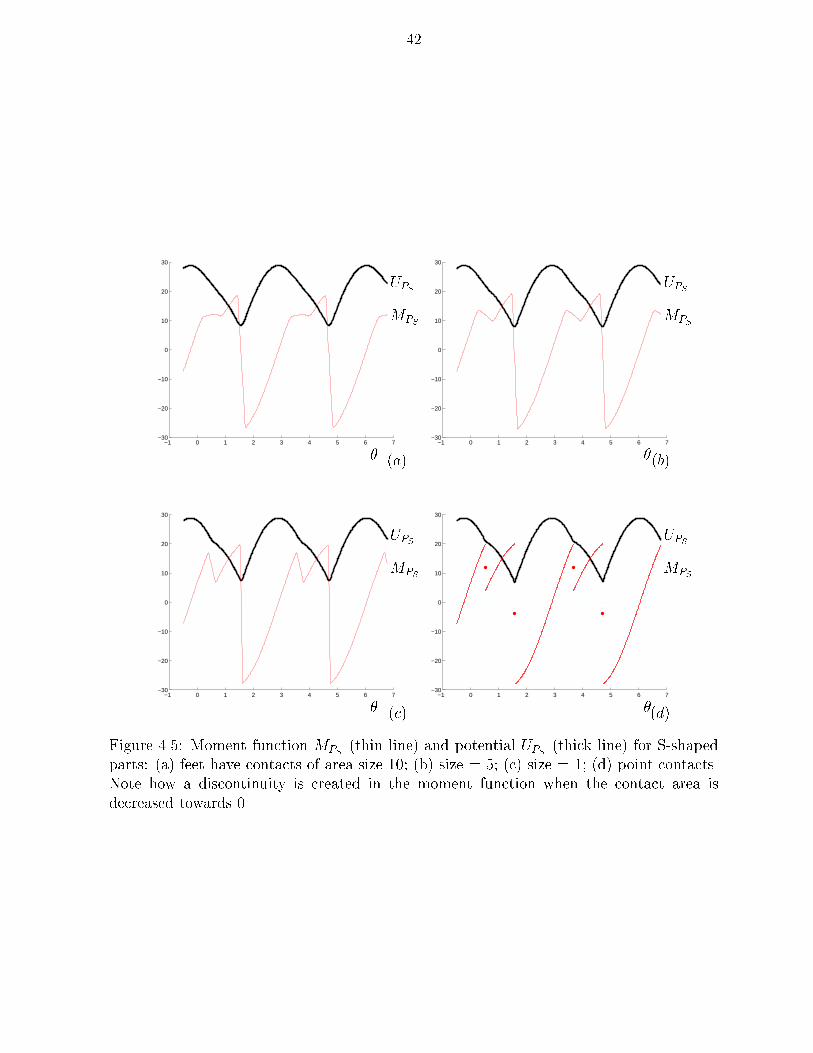
42

−1 0 1 2 3 4 5 6 7−30

−20

−10

0

10

20

30

UPS

MPS

�−1 0 1 2 3 4 5 6 7

−30

−20

−10

0

10

20

30

UPS

MPS

�(a) (b)

−1 0 1 2 3 4 5 6 7−30

−20

−10

0

10

20

30

UPS

MPS

�−1 0 1 2 3 4 5 6 7

−30

−20

−10

0

10

20

30

UPS

MPS

�(c) (d)

Figure 4.5: Moment function MPS (thin line) and potential UPS (thick line) for S-shapedparts: (a) feet have contacts of area size 10; (b) size = 5; (c) size = 1; (d) point contacts.Note how a discontinuity is created in the moment function when the contact area isdecreased towards 0.

43

of vector �elds, and we will write \f ; g" for the resulting continuously varying �eld.By restricting f and g to be �elds with potentials U and V , we know that U + V and(1 � t)U + tV are potential �elds, and hence we can guarantee that f + g and f; g arewell-behaved strategies. These form the basis of our new algorithms in Section 5.

Let us formalize the previous paragraphs. If f is a vector �eld (in this case a squeezepattern) that is applied to move part P , we de�ne the equilibrium set EP (f) as the subsetof the con�guration space C for which P is in equilibrium. Let us write f � g for a strategythat �rst applies vector �eld f , and then vector �eld g to move part P . f + g can beunderstood as applying f and g simultaneously. We have shown that in general EP (f) isnot �nite, but for two orthogonal squeezes f and g, the discrete switching strategy f � gyields a �nite equilibrium set EP (f �g) (see Section 5.2, Claim 39). Furthermore, for someparts the equilibrium is unique up to symmetry.

We wish to explore the relationship between equilibria in simple vector �elds EP (f) orEP (g), combined �elds EP (f + g), discretely-switched �elds EP (f � g), and continuouslyvarying �elds EP (f;g). For example, one may ask whether there exists a strategy withcombined vector �elds, or continuously varying �elds, that, in just one step, reaches thesame equilibrium as a discretely switched strategy requiring multiple steps. Finally, letf1 � f2 � � � � � fs be a sequence of squeeze �elds guaranteed to uniquely orient a part Punder assumption 2Phase. We wish to investigate how continuously varying strategiessuch as f1; f2; � � �; fs can be employed to dynamically achieve the same equilibriaeven when 2Phase is relaxed. The distributed actuation strategy F �G is distributed inspace, but not in time. The strategy F +G is parallel with respect to space and time, sinceF and G are simultaneously \run." Research in this area could lead to a theory of paralleldistributed manipulation that describes spatially distributed manipulation tasks that canbe parallelized over time and space by superposition of controls.

4.3 Upward-Shaped Potential Fields

So far we have presented speci�c force �elds that always (e.g. squeeze and radial �elds) ornever (e.g. skewed squeeze �elds) induce stable equilibria on certain classes of parts. Weconclude this section with a criterion that provides a su�cient condition on force �eldssuch that all parts of a certain size reach a stable equilibrium.

We have observed in Section 3 that a priori it is not obvious when a force �eld inducesstable equilibria. Our Equilibrium Criterion will be based on two important properties:

1. The �eld has a potential. Potential �elds do not allow closed paths (technically, limitcycles) along which the work is positive, which could induce in�nite motion of a part.

2. The force �eld is \inward-directed," which implies that (assuming �rst-order dy-namics) parts can never leave a certain region R. This useful property is a directconsequence of the de�nition of inward-directedness. An inward-directed force �eldcorresponds to an \upward-shaped" potential, in which all paths that leave region Rhave an ascending slope.

We will require Property (1.) to hold for the entire force �eld, while Property (2.)devolves to a boundary condition.

4.3.1 Elementary De�nitions

De�nition 26 Let z 2 Rn. The �-ball around z, denoted B�(z), is the set fr 2 R

n j

44

jr� zj < �g of all points within a distance � of z.

De�nition 27 (Lozano-P�erez [LP83]) Let A, B be sets in Rn. The Minkowski sum

A� B of two sets A and B is de�ned as the set fa + b j a 2 A;b 2 Bg.From these de�nitions it follows that for a region R with boundary @R, the set @R �

Bd(0) = fr + z j r 2 @R; and jzj � dg comprises all points that are within a distance dfrom the boundary of R.

De�nition 28 Given a region R � Rn, de�ne the set CI(R; d) = R� (@R�Bd(0)) which

is the region R shrunk by distance d. Note that CI(R; d) is based upon the con�gurationspace interior [LP83] of R for Bd(0). Abusing terminology slightly, we call CI(R; d) thecon�guration space interior of R in this thesis.

De�nition 29 The radius rP of a part P is the maximum distance between an arbitrarypoint of P and the center of mass (COM) of P .

4.3.2 Equilibrium Criterion

We are now able to state a general criterion for a force �eld f to induce stable equilibriaon all parts in a region S. As mentioned at the beginning of Section 4.3, this criterion isbased on two main conditions: (1) if f has a potential, limit cycles with positive energygain are avoided inside S. (2) if f is \inward-directed" (see the de�nition below), partscannot leave the region S.

In the following we give a general de�nition of inward-directed vector �elds on a man-ifold Z. We then specialize the de�nition to the special instances of Z = C = R

2 � S1

(the con�guration space) and Z = R2, and give a su�cient, practical condition for inward-

directed vector �elds. We conclude with the presentation of the Equilibrium Criterion.De�nition 30 (Inward-Directed Force Fields) 1 Let Z be an arbitrary smooth man-ifold, and let Y � Z be a compact and smooth submanifold with boundary of Z. Assumethat @Y has codimension 1 in Z, and that the boundary of Y is orientable. Let q 2 @Y bea point on the boundary of Y , and Vq 2 TqZ be a tangent vector to Z at q.

We say Vq is inward-directed to @Y at q if there exists a su�ciently small � > 0 suchthat q + �Vq 2 Y .

Let V be a vector �eld on Z. We say V is inward-directed to @Y if V (q) is inward-directed to @Y at q for all q 2 @Y .

Assume the set S � R2 is compact and smooth. Consider the part P when it is placed

into the force �eld f such that its COM lies in S. The set of all such poses is a subsetof the con�guration space C = R

2 � S1 which we call eS = S � S

1. The boundary of eSis @ eS = @S � S

1. Note that @ eS separates the interior i eS = eS � @ eS from the exteriorC � eS = (R 2 � S)� S

1, and that @ eS is isomorphic to a torus S1 � S1.

Now let z = (x; y; �) 2 @ eS, and let Fz 2 TzC represent the lifted generalized forceacting on part P in pose z. Fz is inward-directed (with respect to @ eS) if Fz points intothe interior of eS. Note that this condition is equivalent to saying that the projection of Fz

onto the tangent space at (x; y) to R 2 points into S, because the rotational component of

1In this de�nition, for convenience we assume that Z is embedded in Rm

for some m. This conditionmay be relaxed.

45

Fz is tangential to @ eS. So for example, if z = (x; y; �) 2 @ eS, then z0 = (x; y; �0) 2 @ eS forany �0.

The following proposition gives a simple condition on a force �eld f that tells us if, fora given part P , its lifted generalized force �eld FP is inward-directed:

Proposition 31 Let P be a part with radius r whose COM is the reference point used tode�ne its con�guration space C = R

2�S1. Let f be a force vector �eld de�ned on a region

R � R2, with FP the corresponding lifted generalized force �eld. Let S � R

2 be a convex,compact, and smooth subset of the con�guration space interior of R, and S � CI(R; r).

Consider a point q 2 @S with outward normal nq, and a ball Br(q) with radius r aboutq. If for every point q 2 @S, and for every point s in the corresponding ball Br(q), thedot product g(s) = f(s) � nq is less than 0, then the lifted generalized force �eld FP isinward-directed to @ eS (note: ( � ) is the standard inner product).

Proof: Consider the part P in pose z = (x; y; �) 2 @ eS such that q = (x; y). P has radiusr, hence it lies completely inside the ball Br(q), independent of its orientation �. As weknow that g(p) = f(p) � nq < 0 for all p 2 Br(q), we can conclude that the integral of g(p)

over P is also less than 0:ZPg(p) dA =

ZPf(p) �nq dA = fP �nq < 0. This implies that for

fP , which is the translational component of FP (see De�nition 16), the vector q + � fP (z)lies inside S, if � is positive and su�ciently small. As mentioned on page 44 above, thissu�ces to ensure that the vector z + � FP (z) lies inside eS. 2

Lemma 32 (Equilibrium Criterion) Let P be a polygonal part with radius r, let f bea force �eld with potential U de�ned on a region R � R

2, and let S � R as speci�ed inProposition 31. Let us also assume that the motion of part P is governed by �rst-orderdynamics.

If the lifted force vector �eld FP is inward-directed to @ eS, then the part P will reach astable equilibrium under f in i eS whenever its COM is initially placed in S.

Proof: Assume that the COM of part P is placed at a point (x; y) 2 S. This means thatP is in some pose z = (x; y; �) 2 eS. We now show that the COM of P cannot leave Swhen initially placed inside S. We know that @ eS separates i eS from C � eS. Hence everypath from z to some z� 2 C � eS must intersect @ eS at some point z0 2 @ eS. Now considerpart P in pose z0. Under �rst-order dynamics, its velocity must be in direction of FP (z

0).Because FP is inward-directed, the velocity of P must be towards i eS. In particular, thismeans that the COM will move into iS, hence P cannot leave S, and that there is noequilibrium on @S.

f , and hence (because of Proposition 17) FP have potential U and UP , respectively.Therefore limit cycles with energy gain are not possible. Furthermore, UP ( eS) is the con-tinuous image of a compact set, eS. Therefore the image UP ( eS) is a compact subset of R ,hence has a minimum value attained by some point s 2 eS. Since f is inward-directed, smust lie in i eS. This minimum is a stable equilibrium of P in f , as shown in Corollary 25.2

Because of Lemma 32, the use of potential �elds is invaluable for the analysis of e�ectiveand e�cient manipulation strategies, as discussed in the following section. In particular,it is useful for proving the completeness of a manipulation planner.

Chapter 5

New and Improved Manipulation

Algorithms

The part alignment strategies in Section 2.3 have switch points in time where the vector�eld changes discontinuously (Figure 2.8). We can denote such a switched strategy byf1 � f2 � � � � � fs, where the fi are vector �elds. In Section 2.3 we showed that a generalsqueeze strategy to align a (non-convex) polygonal part with n vertices may need up toO(k n2) switches, and require O(k2 n4) time in planning (k is the maximum number ofpolygon edges that a bisector can cross). To improve these bounds, we now consider abroader class of vector �elds including simple squeeze patterns, radial, and combined �eldsas described in Section 4.

In Section 5.1 we show how, by using radial and combined vector �elds, we can sig-ni�cantly reduce the complexity of the strategies from that of Section 2. In Section 5.2we describe a general planning algorithm that works with a limited \grammar" of vector�elds (and yields, correspondingly, less favorable complexity bounds).

5.1 Radial Strategies

Consider a part P in a force �eld f . Some force �elds exhibit rotational symmetry prop-erties that can be used to generate e�cient manipulation strategies:

Property 33 There exists a unique pivot point v of P such that P is in translationalequilibrium if and only if v coincides with 0.

Property 34 There exists a unique pivot point v of P such that P is in (neutrally stable)orientational equilibrium if and only if v coincides with 0.

We typically think of the pivot point v being a point of P ; however, in generality, just likethe center of mass of P , v does not need to lie within P , but instead is some �xed pointrelative to the reference frame of P . Now consider the part P in an ideal unit radial forcevector �eld R as described in Section 4.

Proposition 35 In a unit radial �eld R, Properties 33 and 34 hold.

46

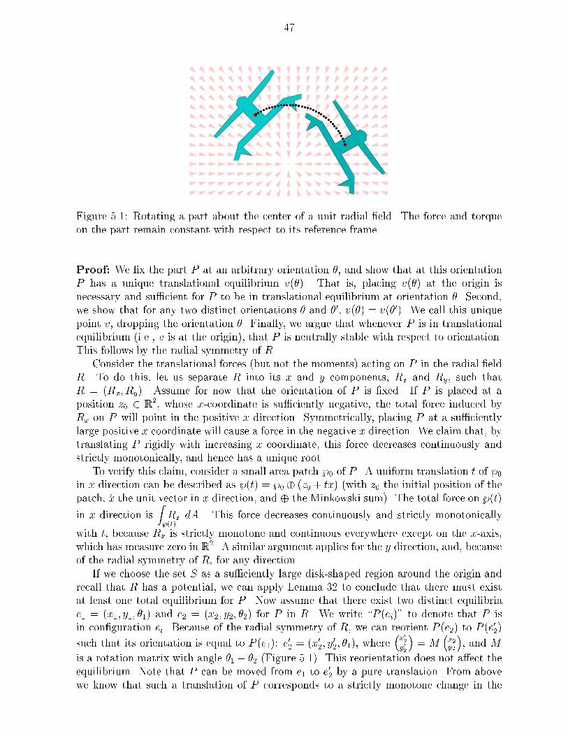
47

Figure 5.1: Rotating a part about the center of a unit radial �eld. The force and torqueon the part remain constant with respect to its reference frame.

Proof: We �x the part P at an arbitrary orientation �, and show that at this orientationP has a unique translational equilibrium v(�). That is, placing v(�) at the origin isnecessary and su�cient for P to be in translational equilibrium at orientation �. Second,we show that for any two distinct orientations � and �0, v(�) = v(�0). We call this uniquepoint v, dropping the orientation �. Finally, we argue that whenever P is in translationalequilibrium (i.e., v is at the origin), that P is neutrally stable with respect to orientation.This follows by the radial symmetry of R.

Consider the translational forces (but not the moments) acting on P in the radial �eldR. To do this, let us separate R into its x and y components, Rx and Ry, such thatR = (Rx; Ry). Assume for now that the orientation of P is �xed. If P is placed at aposition z0 2 R

2, whose x-coordinate is su�ciently negative, the total force induced byRx on P will point in the positive x direction. Symmetrically, placing P at a su�cientlylarge positive x coordinate will cause a force in the negative x direction. We claim that, bytranslating P rigidly with increasing x coordinate, this force decreases continuously andstrictly monotonically, and hence has a unique root.

To verify this claim, consider a small area patch }0 of P . A uniform translation t of }0

in x direction can be described as }(t) = }0 � (z0 + tx̂) (with z0 the initial position of thepatch, x̂ the unit vector in x direction, and � the Minkowski sum). The total force on }(t)

in x direction isZ}(t)Rx dA . This force decreases continuously and strictly monotonically

with t, because Rx is strictly monotone and continuous everywhere except on the x-axis,which has measure zero in R 2. A similar argument applies for the y direction, and, becauseof the radial symmetry of R, for any direction.

If we choose the set S as a su�ciently large disk-shaped region around the origin andrecall that R has a potential, we can apply Lemma 32 to conclude that there must existat least one total equilibrium for P . Now assume that there exist two distinct equilibriae1 = (x1; y1; �1) and e2 = (x2; y2; �2) for P in R. We write \P (ei)" to denote that P isin con�guration ei. Because of the radial symmetry of R, we can reorient P (e2) to P (e

02)

such that its orientation is equal to P (e1): e02 = (x02; y

02; �1), where

�x02y02

�= M

�x2y2

�, and M

is a rotation matrix with angle �1 � �2 (Figure 5.1). This reorientation does not a�ect theequilibrium. Note that P can be moved from e1 to e

02 by a pure translation. From above

we know that such a translation of P corresponds to a strictly monotone change in the

48

translational forces acting on P . Hence we conclude that P (e1) and P (e02) cannot both bein translational equilibrium unless e1 and e02 are equal. This implies that e1 and e2 cannotboth be equilibria of P in R unless they both have the same pivot point v. 2

Surprisingly, v need not be the center of area of P . For example, consider again thepart in Figure 2.5, which consists of a large and a small square connected by a long rod ofnegligible width. The pivot point of this part will lie inside the larger square. But if therod is long enough, the center of area will lie outside of the larger square. However, thefollowing corollary holds:

Corollary 36 For a part P in a continuous radial force �eld R0 given by R0(z) = �z, thepivot point of P coincides with the center of area of P .

Proof: The force acting on P in R0 is given by F =ZP� z dA, which is also the formula

for the (negated) center of area. 2

Now suppose that R is combined with a unit squeeze pattern S, which is scaled by afactor � > 0, resulting in R + �S. The squeeze component �S of this �eld will cause thepart to align with the squeeze, similarly to the strategies in Section 2.3. But note thatthe radial component R keeps the part centered in the force �eld. Hence, by keeping Rsu�ciently large (or � small), we can assume that the pivot point of P remains within an�-ball of the center of R. This implies that assumption 2Phase (see Section 2.3) is nolonger necessary. Moreover, � can be made arbitrarily small by an appropriate choice of �.

Proposition 37 Let P be a polygonal part with n vertices, and let k be the maximumnumber of edges that a bisector of P can cross. Let us assume that v, the pivot point ofP , is in general position. There are at most O(k n) stable equilibria in a �eld of the formR + �S if � is su�ciently small and positive.

Proof: For a part in equilibrium in a pure radial �eld R (i.e., with � = 0), the pivot pointv is essentially �xed at the origin. This is implied by Property 33. It is easy to see thatProperty 33 is not true in general for arbitrary �elds of the form R + �S. Property 33holds if � = 0, because then any orientation is an equilibrium when v is at the center ofR. However, Property 34 does not hold if � > 0, because in general there does not exist aunique pivot point in squeeze �elds (see Section 2.3).

We will conduct the combinatorial analysis of the orientation equilibria under the as-sumptions that (i) � > 0 and (ii) that v is �xed at the origin. Then we will relax the latterassumption (ii), and show that Property 33 holds, approximately, even in R + �S, for asu�ciently small � > 0. That is, we show that a su�ciently small � can be chosen so thatthe combinatorial analysis is una�ected when assumption (ii) is relaxed.

First, we show that when � is small but positive, and with v �xed at the center of R,there are only a linear number of orientation equilibria. (I.e., we constrain the pivot pointv to remain �xed at the origin until further notice.) So let us assume that we are in acombined radial and small squeeze �eld R + �S.

Consider a ray w(0) emanating from v. Assume w.l.o.g. that v is not a vertex of P ,and that w(0) intersects the edges S(0) = fe1; � � � ; ekg of P in general position, 1 � k � n.Parameterize the ray w(�) by its angle � to obtain w(�). As � sweeps from 0 to 2�, eachedge of P will enter and leave the crossing structure S(�) exactly once. S(�) is updatedat critical angles where w(�) intersects a vertex of P . Since there are n vertices, there areO(n) critical angles, and hence O(n) changes to S(�) overall. Hence, since between critical

49

angles S(�) is constant, we see that S(�) takes on O(n) distinct values. Now place thesqueeze line l to coincide with w(�). For a given crossing structure S(�)[S(�+�), satisfyingconditions I and II as de�ned in Section 2.3 devolves to solving two equations. The �rstequation provides the condition for translational equilibrium, while the second equationimplements the condition for orientational equilibrium. The latter equation is called themoment function M(�), because it describes the moment acting on P as a function of �.(But note that M is di�erent from the moment function de�ned in Section 2.3, becausehere the part rotates about a �xed pivot point.) In analogy to Section 2.3 it can be shownthat these equations are algebraic and of degree k, where k is the maximum number ofedges intersected by the squeeze line as described in Section 2.2. This implies that betweenany two adjacent critical values there are only O(k) orientations of l (given by w(�)) thatsatisfy conditions I and II. Hence, the overall number of orientations satisfying I and IIis O(k n).

If � > 0 the part P will be perturbed, so that Property 33 is only approximatelysatis�ed. (That is, we now relax the assumption that v is constrained to be at the origin).However, we can ensure that v lies within an �-ball around the origin (the center of theradial �eld). To see this, �rst consider P at some arbitrary con�guration z in the squeeze

�eld �S. The total squeeze force on Pz is given by the area integral �SP (z) =ZPz�S dA.

(Recall that SP denotes the lifted force �eld of S; see De�nition 16, Equation (4.2).) Now,�SP is bounded above by j�SP j � �A, where A is the area of P (note that S is a unitsqueeze �eld).

P is in equilibrium with respect to the radial �eld R if v is at the origin. Now considerthe lifted force RP when the pivot point of P is not at the origin. More speci�cally, letvz be the pivot point of Pz, and let us de�ne a set RP (d) = fjRP (z)j such that jvzj = dg.We also de�ne a function bRP (d) = minfRP (d)g. This function is well-de�ned, becauseRP (d) is the continuous image of a compact set, hence the minimum exists. bRP (d) is theminimum magnitude of the lifted force acting on Pz when its pivot point vz is at distanced from the origin.

By decomposing RP into its x- and y-components, we can write jRP j asqR2P;x +R2

P;y.

Because of the radial symmetry of R let us assume w.l.o.g. that vz = (d; 0). From the proofof Proposition 35 we know that, for any given orientation of Pz, the magnitude of RP;x

increases continuously and strictly monotonically with increasing d � 0. Furthermore, RP;y

is continuous in d, and RP;y(0) = 0, so R2P;y is continuous and monotonically increasing for

all d less than some su�ciently small d0 > 0. Hence for any �xed orientation of Pz, RP isa continuous and strictly monotonically increasing function for all d 2 [0; d0].

Now suppose that bRP (d) is not strictly monotone, i.e. that there exist d1; d2 with0 � d1 < d2, but bRP (d1) � bRP (d2). Then there must exist z1; z2 with jvz1 j = d1 andjvz2 j = d2, and jRP (z1)j = bRP (d1) � bRP (d2) = jRP (z2)j. Let us de�ne z02 such thatz02;� = z2;� and vz02 = c vz2 for some c 2 R , i.e., vz2 and vz02 lie on a line through theorigin. If we choose 0 � c < 1 then jRP (z

02)j < jRP (z2)j because jRP j is monotone, as

shown in the previous paragraph. In particular, if we choose c = d1=d2, then jRP (z02)j <

jRP (z2)j � jRP (z1)j = bRP (d1), and jvz02 j = jvz1 j. This is a contradiction to the de�nition

of bRP (d1) = minfRP (d)g. We conclude that bRP is continuous and strictly monotone forsu�ciently small d � 0.

Now consider Pz in the combined �eld R + �S, and again let d denote the distancebetween pivot point vz and the origin. In equilibrium the lifted forces RPz and �SPz

50

balance out, hence bRP (d) � jRPzj = j�SPzj � �A, with A the area of P . Since bRP iscontinuous and strictly monotone in d for su�ciently small d, we can ensure that d is lessthan a given �, by chosing an appropriately small �. This implies that vz must lie within an�-ball of the center of the radial �eld. In particular, we can make this �-ball small enoughso that the crossing structure S(�) is not a�ected.

Finally we have to ensure that the stable equilibria, as predicted by the moment functionM , are approximated arbitrarily closely. This means that the disturbance in the momentfunction, caused by pivot point vz not exactly coinciding with the center of the radial�eld, can be made arbitrarily small. To see this, �rst consider the original (unperturbed)moment function M which describes the moment acting on the part P if its pivot pointcoincides with the origin. In this case, the moment is caused solely by the squeeze �eld�S, while P is in equilibrium with respect to the radial �eld R.

Now consider the disturbance in M if the pivot point vz is not exactly at the origin,but somewhere in an �-ball around it. Let us call this disturbance �M , and note that �Mhas two components: �M�S , which is the change in moment caused by the squeeze �eld�S, and �MR, the disturbance caused by the radial �eld R.

For a part P at a given orientation, any �-displacement of vz can change the force ina squeeze �eld �S by at most j�F�S j � � � dP , where dP is the maximum diameter of P .Hence �M�S = r � �F�S is proportional to the product of the disturbance in location �and the magnitude of the squeeze �eld � (r is the �xed distance between pivot point andCOM of P ), i.e. j�M�S j = O(� �).

Since the force caused by the radial �eld R balances the force generated by the squeeze�eld �S, we obtain the same bounds for �MR. We see that �M = �M�S+�MR = O(� �).Recall that � decreases strictly monotonically with �, hence �M decreases asymptoticallyfaster than �. This ensures that we can �nd a su�ciently small � such that the momentfunction M is approximated arbitrarily closely, and the equilibria of the squeeze �eld �Sare not a�ected.

We conclude that the number of equilibria in a �eld R+ �S is bounded by O(k n), forsu�ciently small �. 2

In analogy to Section 2.3 we de�ne the turn function t : S1 ! S1, which describes

how the part will turn under a squeeze pattern, and hence yields the stable equilibriumcon�gurations. Given the turn function t we can construct the corresponding squeezefunction s as described in Section 2.3. With s as the input for Goldberg's alignmentplanner [Gol93], we obtain strategies for unique part alignment (and positioning) of lengthO(k n). They can be computed in time O(k2 n2).

The result is a strategy for parts positioning of the form (R+ �S1) � � � �� (R+ �SO(kn)

).Compared to the general squeeze algorithm in Section 2.3, it improves the plan length by afactor of n, and the planning complexity is reduced by a factor of n2. The planner is com-plete: For any polygonal part, there exists a strategy of the form �i(R+�Si). Moreover, thealgorithm is guaranteed to �nd a strategy for any input part. By appending a step whichis merely the radial �eld R without a squeeze component, we are guaranteed that the partP will be uniquely posed (v is at the origin) as well as uniquely oriented. We can also showthat the continuously varying \morphing" strategy (R+ �S1) ; � � �; (R+ �S

O(kn)) ; R

works in the same fashion to achieve the same unique equilibrium.

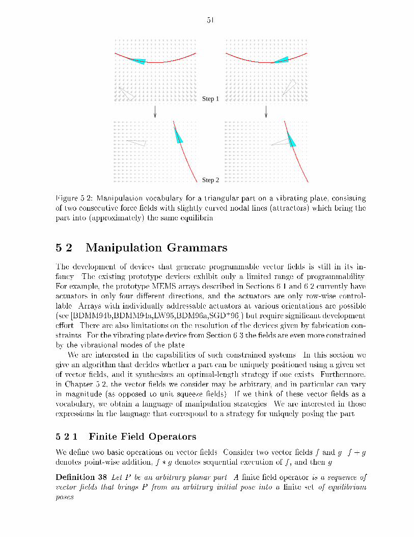
51

Step 1

Step 2

Figure 5.2: Manipulation vocabulary for a triangular part on a vibrating plate, consistingof two consecutive force �elds with slightly curved nodal lines (attractors) which bring thepart into (approximately) the same equilibria.

5.2 Manipulation Grammars

The development of devices that generate programmable vector �elds is still in its in-fancy. The existing prototype devices exhibit only a limited range of programmability.For example, the prototype MEMS arrays described in Sections 6.1 and 6.2 currently haveactuators in only four di�erent directions, and the actuators are only row-wise control-lable. Arrays with individually addressable actuators at various orientations are possible(see [BDMM94b,BDMM94a,LW95,BDM96a,SGD+96]) but require signi�cant developmente�ort. There are also limitations on the resolution of the devices given by fabrication con-straints. For the vibrating plate device from Section 6.3 the �elds are even more constrainedby the vibrational modes of the plate.

We are interested in the capabilities of such constrained systems. In this section wegive an algorithm that decides whether a part can be uniquely positioned using a given setof vector �elds, and it synthesizes an optimal-length strategy if one exists. Furthermore,in Chapter 5.2, the vector �elds we consider may be arbitrary, and in particular can varyin magnitude (as opposed to unit squeeze �elds). If we think of these vector �elds as avocabulary, we obtain a language of manipulation strategies. We are interested in thoseexpressions in the language that correspond to a strategy for uniquely posing the part.

5.2.1 Finite Field Operators

We de�ne two basic operations on vector �elds. Consider two vector �elds f and g. f + gdenotes point-wise addition, f � g denotes sequential execution of f , and then g.

De�nition 38 Let P be an arbitrary planar part. A �nite �eld operator is a sequence ofvector �elds that brings P from an arbitrary initial pose into a �nite set of equilibriumposes.

52

A �eld operator comes with the following guarantee: No matter where in R 2�S1 the part

starts o�, it will always come to rest in one of E di�erent total equilibria (Figure 5.2).That is: for any polygonal part P , either of these �eld operators is always guaranteed toreduce P to a �nite set of equilibria in its con�guration space C = R

2 � S1.

From Section 5.1 we know that combined radial-squeeze patterns R + �S have thisproperty. However, there are other simple �eld operators that also have this �nitenessproperty:

Claim 39 [BDM96b] Let f and f? be unit squeeze �elds such that f? is orthogonal to f .Then the �elds f � f? and f + f? induce a �nite number of equilibria on every connectedpolygon P , hence f � f? and f + f? are �nite �eld operators.

Proof: First consider the �eld f � f?, and w.l.o.g. assume that f(x; y) = (�sign(x); 0).Also assume that the COM of P is the reference point used to de�ne its con�guration spaceC = R

2 � S1. As discussed in Sections 2.2 and 2.3, P will reach one of a �nite number of

orientation equilibria when placed in f or f?. More speci�cally, when P is placed in f ,there exists a �nite set of equilibria Ef = f(xi; �i)g, where xi is the o�set from f 's squeezeline, and �i is the orientation of P (see Section 2.5). Similarly for f?(x; y) = (0;�sign(y)),there exists a �nite set of equilibria Ef? = f(yj; �j)g. Since the x-component of f? is zero,the x-coordinate of the reference point of P (the COM) remains constant while P is in f?.Hence P will �nally come to rest in a pose (xk; yk; �k), where xk 2 �1(Ef), (yk; �k) 2 Ef?,and �1 is the canonical projection such that �1(x; �) = x. Since Ef is �nite, so is �1(Ef ).E(f?) is also �nite, therefore there exists only a �nite number of such total equilibriumposes for f � f?.

If P is placed into the �eld f+f?, there exists a unique translational equilibrium (x; y)for every given, �xed orientation �. In each of these translational equilibria, the squeezelines of f and f? are both bisectors of P . Now consider the moment acting on P when P isin translational equilibrium as a function of �. Since there are O(n2) topological placementsfor a single bisector, therefore there exist also only O(n2) topological placements for twosimultaneous, orthogonal bisectors. In analogy to Proposition 4 in Section 2.2 we can showthat for any topological placement of the bisectors, this moment function has at most O(k)roots, where k is the maximum number of edges a bisector of P can cross. This impliesthat there exist only O(k n2) distinct total equilibria for f + f?. 2

Corollary 40 Let f be a �nite �eld operator for a part P , and let g be an arbitrary vector�eld. Then the sequence g � f is a �nite �eld operator.

Proof: By de�nition of a �nite �eld operator, f brings the part P into a �nite set ofequilibrium poses from arbitrary initial poses, in particular from the poses that are theresult of �eld g. 2

Thus by pre-pending an arbitrary sequence of �elds to a �nite �eld operator, one canalways create a new �nite �eld operator (possibly with a smaller set of discrete equilibria).In the remainder of this section, however, we will only consider �nite �eld operators ofminimal length, i.e. �eld sequences from which no �eld can be removed without losing the�niteness property (De�nition 38).

We have seen in Sections 2 and 4 that for simple force �elds such as e.g. squeeze orradial �elds, we can predict the motion and the equilibria of a part with exact analyticalmethods. However, for arbitrary �elds (e.g. the force �elds described in Section 6.3 which

53

are induced by vibrating plates), such algorithms are not known. Instead we can employapproximate methods to predict the behavior of the part in the force �eld. These methodsare typically numerical computations that involve simulating the part from a speci�c initialpose, until it reaches equilibrium.1 We call the cost for such a computation the simulationcomplexity s(n). We write s(n) because the simulation complexity will usually depend onthe complexity of the part, i.e., its number of vertices n (for more details also see [DX95]).

Proposition 41 [BDM96b] Consider a polygonal part P , and m �nite �eld operatorsfFig, 1 � i � m, each with at most E distinct equilibria in the con�guration space C for P .There is an algorithm that generates an optimal-length strategy of the form F1 �F2 � � � ��Fl

to uniquely pose P up to symmetries, if such a strategy exists. This algorithm runs inO(m2E (s(n) + 2E)) time, where s(n) is the simulation complexity of P in Fi. If no suchstrategy exists, the algorithm will signal failure.

Proof: Construct a transition table T of size m2E that describes how the part P movesfrom an equilibrium of Fi to an equilibrium of Fj. This table can be constructed either bya dynamic analysis similar to Section 2.1, or by dynamic simulation. The time to constructthis table is O(m2E s(n)), where s(n) is the simulation complexity, which will typicallydepend on the complexity of the part.

Using the table T , we can search for a strategy as follows: De�ne the state of thesystem as the set of possible equilibria a part is in, for a particular �nite �eld operator Fi.There are O(E) equilibria for each �nite �eld operator, hence there are O(m 2E) distinctstates. For each state there are m possible successor states as given by table T , and theycan each be determined in O(E) operations, which results in a graph with O(m 2E) nodes,O(m22E) edges, and O(m2E 2E) operations for its construction. Finding a strategy, ordeciding that it exists, then devolves to �nding a path whose goal node is a state with aunique equilibrium. The total running time of this algorithm is O(m2E (s(n) + 2E)). 2

Hence, as in [EM88], for any part we can decide whether a part can be uniquelyposed using the vocabulary of �eld operators fFig but (a) the planning time is worst-case exponential and (b) we do not know how to characterize the class of parts that canbe oriented by a speci�c family of operators fFig. However, the resulting strategies areoptimal in length.

This result illustrates a tradeo� between mechanical complexity (the dexterity andcontrollability of �eld elements) and planning complexity (the computational di�culty ofsynthesizing a strategy). If one is willing to build a device capable of radial �elds, then onereaps great bene�ts in planning and execution speed. On the other hand, we can still planfor simpler devices (see Figures 1.4 and 5.2), but the plan synthesis is more expensive, andwe lose some completeness properties.

5.2.2 Example: Uniquely Posing Planar Parts

In this section we will show how to accomplish tasks with manipulation grammars asdeveloped in Section 5.2.1. Recall from Section 2.3 that we say a manipulation strategyorients (respectively, poses) a part uniquely if from any initial con�guration, the partcan be brought into a unique �nal orientation (respectively, pose). We will show howthe synthesized plans uniquely pose parts from any initial con�guration. As an example,

1See for example URL http://www.cs.cornell.edu/home/karl/Cinema.

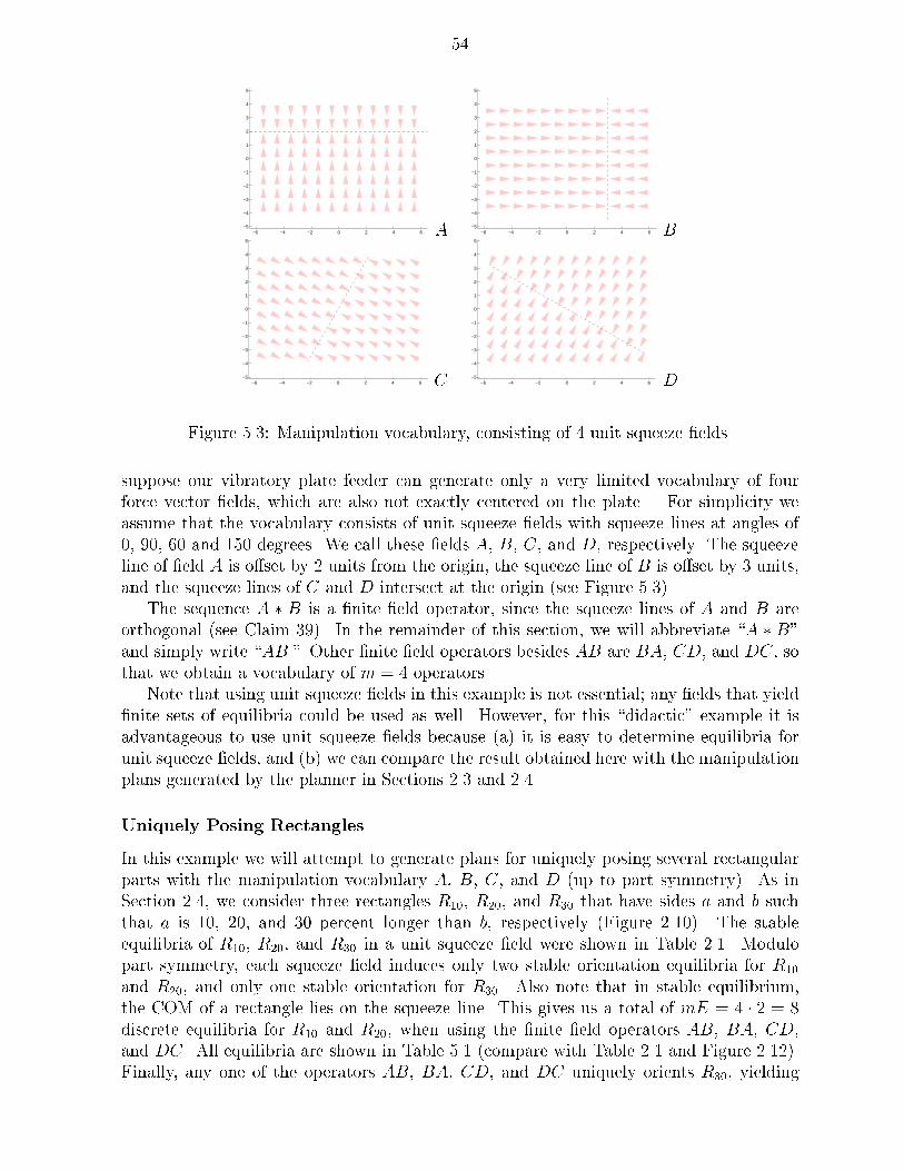
54

−6 −4 −2 0 2 4 6−5

−4

−3

−2

−1

0

1

2

3

4

5

A −6 −4 −2 0 2 4 6−5

−4

−3

−2

−1

0

1

2

3

4

5

B

−6 −4 −2 0 2 4 6−5

−4

−3

−2

−1

0

1

2

3

4

5

C −6 −4 −2 0 2 4 6−5

−4

−3

−2

−1

0

1

2

3

4

5

D

Figure 5.3: Manipulation vocabulary, consisting of 4 unit squeeze �elds.

suppose our vibratory plate feeder can generate only a very limited vocabulary of fourforce vector �elds, which are also not exactly centered on the plate. For simplicity weassume that the vocabulary consists of unit squeeze �elds with squeeze lines at angles of0, 90, 60 and 150 degrees. We call these �elds A, B, C, and D, respectively. The squeezeline of �eld A is o�set by 2 units from the origin, the squeeze line of B is o�set by 3 units,and the squeeze lines of C and D intersect at the origin (see Figure 5.3).

The sequence A � B is a �nite �eld operator, since the squeeze lines of A and B areorthogonal (see Claim 39). In the remainder of this section, we will abbreviate \A � B"and simply write \AB." Other �nite �eld operators besides AB are BA, CD, and DC, sothat we obtain a vocabulary of m = 4 operators.

Note that using unit squeeze �elds in this example is not essential; any �elds that yield�nite sets of equilibria could be used as well. However, for this \didactic" example it isadvantageous to use unit squeeze �elds because (a) it is easy to determine equilibria forunit squeeze �elds, and (b) we can compare the result obtained here with the manipulationplans generated by the planner in Sections 2.3 and 2.4.

Uniquely Posing Rectangles

In this example we will attempt to generate plans for uniquely posing several rectangularparts with the manipulation vocabulary A, B, C, and D (up to part symmetry). As inSection 2.4, we consider three rectangles R10, R20, and R30 that have sides a and b suchthat a is 10, 20, and 30 percent longer than b, respectively (Figure 2.10). The stableequilibria of R10, R20, and R30 in a unit squeeze �eld were shown in Table 2.1. Modulopart symmetry, each squeeze �eld induces only two stable orientation equilibria for R10

and R20, and only one stable orientation for R30. Also note that in stable equilibrium,the COM of a rectangle lies on the squeeze line. This gives us a total of mE = 4 � 2 = 8discrete equilibria for R10 and R20, when using the �nite �eld operators AB, BA, CD,and DC. All equilibria are shown in Table 5.1 (compare with Table 2.1 and Figure 2.12).Finally, any one of the operators AB, BA, CD, and DC uniquely orients R30, yielding

55

Table 5.1: Stable equilibria of rectangular parts R10 and R20 for the manipulation vocab-ulary AB, BA, CD, and DC.

Operator Equilibrium R10 R20

(x; y; �) (x; y; �)

AB 1 (3,2,0.97) (3,2,1.29)2 (3,2,2.18) (3,2,1.85)

BA 3 (3,2,2.54) (3,2,2.86)4 (3,2,0.61) (3,2,0.28)

CD 5 (0,0,2.01) (0,0,2.34)6 (0,0,0.08) (0,0,2.90)

DC 7 (0,0,0.44) (0,0,0.77)8 (0,0,1.65) (0,0,1.33)

Table 5.2: Transition table for equilibria of the rectangles R10 and R20, with �nite �eldoperators AB, BA, CD, and DC. For both rectangles, there exist a total of E = 8equilibria, and m = 4 �nite �eld operators.

R10 R20

to toAB BA CD DC AB BA CD DC

from AB 1 1 4 6 7 1 4 5 82 2 3 5 8 2 3 5 8

BA 3 2 3 5 8 2 3 6 74 1 4 6 7 1 4 6 7

CD 5 2 3 5 8 2 3 5 86 1 4 6 7 2 3 6 7

DC 7 1 4 6 7 1 4 6 78 2 3 5 8 1 4 5 8

trivial one-step plans to uniquely pose R30. Hence we will omit R30 for the remainder ofthis example.

Given the discrete equilibria, the algorithm based on the constructive proof of Propo-sition 41 generates a transition table T that describes the mapping between initial equi-librium pose and �nal equilibrium pose of a part when one �nite �eld operator is applied.This table has mE rows and m columns. Table 5.2 shows the transitions for parts R10

and R20. Each entry in T can be determined either by dynamic analysis, or by simulation.The values in Table 5.2 were generated by our planner using simulation. Figure 5.4 showsa trace of such a simulation: The initial pose of part R20 is equilibrium e3 = (3; 2; 2:86).In �eld C, R20 moves left and up until it reaches an equilibrium on the squeeze line of C.Subsequently, after �eld D is applied, R20 comes to rest in equilibrium e6 = (0; 0; 2:90).In this case, using Claim 39, the equilibria (but not the transitions) can be calculatedanalytically.

Recall from Section 5.2.1 that this system has a state space of size O(m 2E), becausefor each of the m �nite �eld operators, there are O(E) discrete equilibria in which the

56

−6 −4 −2 0 2 4 6−5

−4

−3

−2

−1

0

1

2

3

4

5

−6 −4 −2 0 2 4 6−5

−4

−3

−2

−1

0

1

2

3

4

5

(a) (b)

Figure 5.4: Simulation of part R20 from equilibrium 3 by using �nite �eld operator CD,reaching equilibrium 6: (a) applying �eld C; (b) applying �eld D.

part could be. For example, a state could be \the part is in equilibrium 1, 2, or 4." Wecan represent such a state as a binary string, \11010000." Hence the transition table Tcan be used to de�ne a transition graph whose nodes are the O(m 2E) states, and whoseO(m2E 2E) edges are derived from the mE transitions in T . A simple breadth-�rst searchof this graph, starting from the state in which all equilibria are possible, will yield optimal-length plans to reach any reachable state.2 This algorithm will also decide which statesare unreachable. Hence it can signal success when the shortest plan to reach a state witha unique equilibrium is found, or signal failure if no such plan exists. Figure 5.5 showstransition graphs for parts R10 and R20 with all reachable states, and the shortest pathsto reach them from the initial \generic" state, in which the part has an arbitrary pose.Notice that there exists a two-step plan for uniquely posing R20, but no such plan existsfor R10.

In summary, we observe that with our �nite �eld operators AB, BA, CD, and DC, R30

can be uniquely posed in one step, R20 requires two steps, while there exists no strategy forR10. Recall that the general squeeze algorithm in Section 2.4 found an alignment strategyfor all three rectangles R10, R20 as well as R30. However, the algorithm required twosqueeze �elds at a relative angle of approximately 45�; for R10, it would fail for squeezelines at a relative angle of 60�. Apparently, parts that are closer to rotational symmetry(i.e., in this case, closer to square-shaped) are more di�cult to pose uniquely than moreasymmetric (i.e., long rectangular-shaped) parts.

Uniquely Posing and Feeding Arbitrary Parts

In this section we will demonstrate the manipulation grammar algorithm for a more realisticpart (see Figure 5.6a), and for two di�erent manipulation vocabularies. All strategies in thissection (and Section 5.2.2) were computed using an automatic planner we implemented,using the techniques of Section 5.2.1. We will �rst extend our manipulation grammarby adding a �eld F that has a vertical squeeze line at x = �3 (Figure 5.7 left), whichyields two new �nite �eld operators, AF and FA. Analysis of the part shows that it has

2We could also imagine using A�-search to improve performance.

57

ARBITRARY

11000000

00110000

00001100

00000011DC

CD

BA

AB

ARBITRARY

11000000

00110000

00001100

00000011

00001000

00000001

00000100

00000010

01000000

00100000

10000000

00010000

DC

CD

BA

AB

DC

CD

DC

CD

BA

AB

BA

AB

(a)

(b)

Figure 5.5: Minimum spanning trees of the state transition graphs for rectangles (a) R10,and (b) R20. All reachable states are shown, as well as the shortest paths to reach each ofthem. Non-spanning edges (e.g. an edge CD from 11000000 to 00001100) are omitted forsimplicity.(a) No state with unique equilibrium can be reached for R10.(b) There exist several two-step plans for R20 that reach states with unique equilibrium.(Graphs were generated automatically by our planner software.)

58

(a) −8 −6 −4 −2 0 2 4 6 8

−6

−4

−2

0

2

4

6

(b)

Figure 5.6: Sample part: (a) nonconvex shape with holes; (b) its four stable equilibria ina unit squeeze �eld.

−6 −4 −2 0 2 4 6−5

−4

−3

−2

−1

0

1

2

3

4

5

F −6 −4 −2 0 2 4 6−5

−4

−3

−2

−1

0

1

2

3

4

5

G

Figure 5.7: Extensions to the manipulation vocabulary, consisting of 2 unit squeeze �elds.

4 stable orientation equilibria in a unit squeeze �eld (Figure 5.6b). It is not di�cult tosee that, after any two orthogonal squeezes, the part can be in E = 8 di�erent poses. Weobtain a transition table of size m2E = 228, which results in a state transition graph withm 2E = 1536 nodes (states) and m22E = 9216 edges (transitions). The algorithm �ndsthe following strategy: CD BA AF FA, which is equivalent to CDBAFA. Two sampleexecutions of this strategy are shown in Figure 5.8, from di�erent initial poses. A closelook at the strategy reveals that operator CD approximately centers the part, such that Bcan move the part into one of four discrete orientation equilibria below the squeeze line ofA. Then A reduces the number of orientation equilibria to two, and F to one (at a uniquex-position). Finally, A brings the part into a unique pose: e� � (�2:9; 1:9; 3:6).

It is important to note the following distinction between the general squeeze strategiesfor parts orienting of Section 2.3, and the manipulation grammar strategies: As mentionedin Section 2.3, turn and squeeze functions render planning algorithms based upon themsusceptible to �eld symmetries, thereby introducing aliasing in orientation space and ad-mitting completeness and uniqueness proofs of orientation only modulo �eld symmetry.Since manipulation grammars do not employ turn or squeeze functions, they are immuneto this problem, and parts without rotational symmetry can be posed uniquely. In essence,turn and squeeze functions assume a global �eld symmetry. In manipulation grammars,such �eld symmetries may not exist, e.g. squeeze �elds could have arbitrary angles and

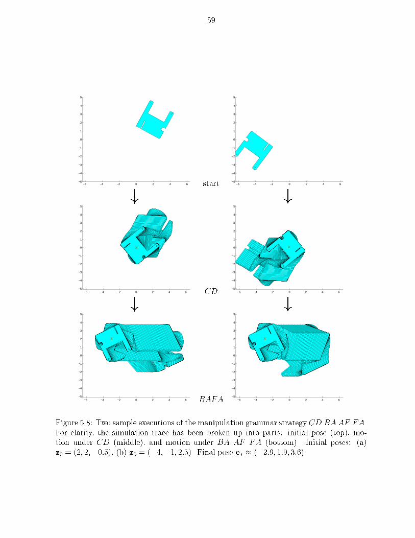
59

−6 −4 −2 0 2 4 6−5

−4

−3

−2

−1

0

1

2

3

4

5

start −6 −4 −2 0 2 4 6−5

−4

−3

−2

−1

0

1

2

3

4

5

# #

−6 −4 −2 0 2 4 6−5

−4

−3

−2

−1

0

1

2

3

4

5

CD −6 −4 −2 0 2 4 6−5

−4

−3

−2

−1

0

1

2

3

4

5

# #

−6 −4 −2 0 2 4 6−5

−4

−3

−2

−1

0

1

2

3

4

5

BAFA −6 −4 −2 0 2 4 6−5

−4

−3

−2

−1

0

1

2

3

4

5

Figure 5.8: Two sample executions of the manipulation grammar strategy CD BA AF FA.For clarity, the simulation trace has been broken up into parts: initial pose (top), mo-tion under CD (middle), and motion under BA AF FA (bottom). Initial poses: (a)z0 = (2; 2;�0:5), (b) z0 = (�4;�1; 2:5). Final pose e� � (�2:9; 1:9; 3:6).

60

o�sets from the origin. In the �rst example of this section (Figure 5.8), the �nal pose isindeed unique.

As a second example, we add the �eld G, which has a horizontal squeeze line at y = �2(Figure 5.7 right), and remove the �elds C and D. This results in 8 �nite �eld opera-tors, hence we obtain m2E = 512 entries in the transition table, m 2E = 2048 states andm22E = 16384 transitions. We obtain the strategy GB BA AF FG, which is equivalentto GBAFG. During execution of this strategy, the COM of the part follows a counter-clockwise rectangular path, at each step reducing the number of possible equilibria, until,in the lower left corner, a unique pose is reached (Figure 5.9). This opens the possibilityof pipelining the posing process, which could yield more e�cient parts feeders: as longas we can ensure that the next part is initially placed su�ciently far to the right so notto interfere with its predecessor, the G �eld can be used simultaneously for two parts.Hence if the parts feeder periodically cycles through the �elds GBAF , the next part canbe introduced into the device each time before G is executed. A part is uniquely posedafter each execution of G.

5.2.3 Summary

In this section we have de�ned manipulation grammars that consist of a vocabulary of pla-nar force vector �elds, and we presented an implemented planning algorithm that generatesstrategies to uniquely position and orient parts. In comparison with the general squeezestrategies of Section 2.3, manipulation grammars allow sets of arbitrary force vector �elds,and are not limited to a 1-parameter family of squeeze �elds. Consequently, dependingon the available manipulation vocabulary, the resulting strategies can be more powerful ormore restricted than the orienting strategies generated by the general squeeze algorithmof Section 2.3. In particular, parts can be uniquely posed even when only symmetric force�elds are available. As a tradeo�, planning and execution complexity is worst-case expo-nential instead of merely quadratic in the number of equilibria of the part, and there existno completeness guarantees that a strategy always exists for a given vocabulary or class ofparts. Moreover, numerical simulation was employed to predict the transitions, whereasthey may be exactly computed (Section 2.3) for simple squeezes.

61

−6 −4 −2 0 2 4 6−5

−4

−3

−2

−1

0

1

2

3

4

5

start −6 −4 −2 0 2 4 6−5

−4

−3

−2

−1

0

1

2

3

4

5

# #

−6 −4 −2 0 2 4 6−5

−4

−3

−2

−1

0

1

2

3

4

5

GB −6 −4 −2 0 2 4 6−5

−4

−3

−2

−1

0

1

2

3

4

5

# #

−6 −4 −2 0 2 4 6−5

−4

−3

−2

−1

0

1

2

3

4

5

AFG −6 −4 −2 0 2 4 6−5

−4

−3

−2

−1

0

1

2

3

4

5

Figure 5.9: Two sample executions of strategy GB BA AF FG = GBAFG. For clarity,the simulation trace has been broken up into parts: initial pose (top), motion under GB(middle), and motion under AFG (bottom). Initial poses: (a) z0 = (1;�3;�0:5), (b)z0 = (4;�1; 2:5). Final pose e� � (�2:9;�1:9; 5:9).

Chapter 6

Experimental Apparatus for

Programmable Force Fields

The theory of programmable vector �elds developed in this thesis arguably represents the�rst systematic attack on massively-parallel distributed manipulation based on geometricand physical reasoning. In this chapter we report on our experiments in implementing thistheory using microfabricated actuator arrays and macroscopic vibrating plates.

6.1 Microfabricated Arrays of Single-Crystal Silicon

Torsional Actuators

A wide variety of MEMS (Micro Electro Mechanical Structures) has been built recentlyby using processing techniques derived from VLSI fabrication. The �rst commercially suc-cessful MEMS structure was the Analog Devices, Inc. single-chip, bulk-fabricated air bagsensor [Ana91]. In this section, we investigate arrays of MEMS actuators that can performmanipulation tasks. There is a large number of possible applications from macroscopic tomicroscopic size scales, such as bulk-fabricated (cheap), ultra-thin transport mechanisms,e.g. for paper in copy machines or printers. At the other end of the scale spectrum, recentadvances have brought within reach arrays equipped with tips that can probe and moveobjects consisting of only a few atoms [XMM95]. Such devices, employed in a massivelyparallel fashion, may yield tremendous data storage capacities.

Various actuation principles for micro actuator arrays and micro manipulation sys-tems have been proposed in recent years. Pister et al. [PFH90] demonstrated a levitationsystem consisting of microfabricated nozzles, and electrostatic actuation. Takeshima andFujita [TF90] introduce the concept of a distributed micro motion system that consistsof an array of cooperating actuator modules. Furuhata et al. [FHF91] have built arraysof ultrasonic microactuators. An integrated, monolithic mirror array for video projectionshas been presented by Sampsell [Sam93]. B�ohringer et al. [BDMM94b] have developed atheory of manipulation and control for micro actuator arrays. Konishi and Fujita [KF93a]use controlled, directed micro air valves to convey small objects. Ataka et al. [AOF93]simulate cilia with thermal bimorph micro structures. Liu and Will [LW95] propose theconcept of intelligent motion surfaces for micro assembly tasks. Liu et al. [LTW+95,LW95]present a micro assembly system based on magnetic actuator arrays. Electrostatic actuatorarrays are described by B�ohringer et al. [BDM96a] and Storment et al. [SBW+94]. Suh et

62

63

(a) (b)

Figure 6.1: Torsional asymmetric actuator with electrode and tips, suspended on a tor-sional rod: (a) CAD model, (b) scanning electron microscopy. Left: Dense grid (10�mspacing) with aluminum electrode underneath. Right: Grid with 5�m high poles.

al. [SGD+96] present an array of thermobimorph micro cilia which are able to accuratelymove and position silicon chips. The MEMS array that we present here is designed forapplications in which objects in the millimeter range are moved, e.g. for a programmablestage of a microscope, or for automated handling and assembly of small parts.

Reznik et al. [RBC97] performed thorough tests of the proposed manipulation strategieswith a sophisticated dynamic simulator [MC95], verifying the predicted behavior of partsby our theory of force vector �elds. Manipulation experiments that support our theory aredescribed by Suh et al. [SGD+96].

Compatibility with standard VLSI processes allows integration of control circuitry onthe same chip. This is of great importance if we want to employ powerful manipulationstrategies that require individual control of the actuators in the array. The SCREAMprocess [ZM92,SZM93] (for Single-Crystal Silicon Reactive Etching and Metallization) isa low temperature process that can be performed after the fabrication of circuits hasbeen completed [SM96]. In the following sections we will discuss design, fabrication, andtesting of a SCREAM electrostatic actuator array (see Figure 1.2), and we discuss controlstrategies for massively-parallel actuator arrays.

Our goal is to generate motion plans at a high (task) level and automatically transformthem into an actuator array control strategy, in analogy to a compiler that translates highlevel instructions into assembler code. We believe that such high level strategies of microsensors and actuators are essential for e�cient control of future complex MEMS systems.Conversely, the availability of high level descriptions for MEMS and micro robotic tasksmay in uence and improve the MEMS design, similarly to the concurrent design of omputerchips and compilers.

6.1.1 Actuator Design

A torsional actuator consists of a rectangular grid etched out of single-crystal silicon sus-pended by two rods that act as torsional springs (Figure 6.1). The design is based ontorsional resonators [MZSM93,MM96]. In our current design, the grid is 180�m long andextends 120 � 180�m on each side of the rod. The rods are 150�m long. The currentasymmetric design has 5� 10�m high protruding tips (Figure 6.2) on one side of the gridthat make contact with an object lying on top of the actuator. The other side of thegrid consists of more densely spaced beams above an aluminum electrode. If a voltage is

64

Figure 6.2: Released actuators consisting of single-crystal silicon with 5�m high tips.

Figure 6.3: Micro motion pixel consisting of actuators oriented in four di�erent directions.

applied between actuator grid and electrode, the half of the grid above the electrode ispulled downward by the resulting electrostatic force. Simultaneously the other side of thegrid (with the tips) is de ected out of the plane by several �m. Hence an object can belifted and pushed sideways by the actuator.

Because of its low inertia (resonance in the high kHz range) the device can be drivenin a wide frequency range from DC to several 100 kHz AC. Due to the asymmetry in theactuator design, each actuator generates motion in one speci�c direction if it is activated;otherwise it acts as a passive frictional contact. Figure 1.2 shows a small portion of sucha unidirectional actuator array, which consists of more than 15,000 individual actuatorsthat densely cover the substrate surface.

The layout of the array can be changed such that the actuators point in various ori-entations. Then the combination and selective activation of several actuators in di�erentorientations (a motion pixel, see Figure 6.3) allows us to generate various motions in dis-

65

crete directions, spanning the plane.

Feasibility Calculations

To answer the question Can microscopic actuators move macroscopic parts? we investi-gate the (vertical) levitation forces generated by the micro actuators. Section 6.1.1 willthen focus on lateral forces that induce motion on the part. Let us consider the speci�cweight (i.e., in this case, the weight per area ratio) of a variety of objects and materials.For example, the speci�c weight of paper is approximately 1N=m2 = 1�N =mm2. A sil-icon wafer is about ten times heavier at 10�N =mm2. We compare these values with theelectrostatic force generated by a parallel-plate capacitor. The force per area ratio can becomputed as F=A = "0V

2=d2, where V is the applied voltage, d is the gap width betweenthe capacitor plates, and "0 is the permittivity of free space. For a gap width of d = 5�mand a voltage of 60V (typical values for our actuators), we obtain a force per area ratio ofapproximately 1:2mN =mm2. This result is more than two orders of magnitude higher thane.g. the speci�c weight of a silicon wafer. Note that the force is proportional to the squareof the applied voltage V as well as the gap width d. Therefore, higher voltages and smallergap sizes will largely improve the e�ectiveness of our electrostatic devices. However, theforce diminishes quickly with larger gap widths, which limits the range of motion of thecurrent actuator design.

Due to fabrication constraints, the electrode of our torsional actuator does not consistof a continuous plate, but rather of a grid of approximately 1�m wide beams spaced at10�m distance. This is necessary to release the structure from the substrate, as well asfor the deposition of an Aluminum electrode underneath the actuator. To investigate theloss in electrostatic force incurred by these design limitations, we have analyzed torsionalactuators using the �nite element simulator Coulomb [Int89]. This analysis shows thatfor the given actuator geometry, the electrostatic force is reduced to about one-third of theforce generated by an ideal parallel-plate capacitor.

Finally, due to layout constraints, not all of the wafer surface can be used for actuators.In a practical layout of a densely packed actuator array, approximately 30% of the chipsurface is covered with electrostatic capacitors. The remaining area is used for the actuatorgrids that support the tips, torsional beams, and electrical connections.

Summarizing the results of the feasibility calculations in this section, we conclude thateven though the e�ective electrostatic force generated by our actuators is only about onetenth of an ideal parallel-plate capacitor, useful manipulation tasks can be performed withelectrostatic micro actuators.

New designs with much higher performance are currently under development. Parallel-plate capacitors can be replaced by torsional comb-drive actuators, which combine verysmall gap widths with theoretically unlimited angular range of motion. Since these highaspect ratio comb drives employ vertical side walls as capacitors, the e�ective capacitorsurface increases signi�cantly. In particular, it can be larger than the (two-dimensional)chip area. Smaller gap sizes and larger surface areas will result in an increase in electrostaticforce by several orders of magnitude.

Design of SCS Torsional Actuators

In this section we investigate the generation of lateral motion based on a kinematic analysisof torsional actuators, which will yield design rules to optimize actuator design. Calcula-

66

θ b

a

h

d

Figure 6.4: Schematic cross section of torsional actuator (not to scale): Actuator width(from torsional axis) a and b, height of tips h, gap width between actuator and electroded, and torsional de ection �.

tions show that the mass of an individual actuator is less than 100 ng; by comparison, themass of a typical object that we want to move (paper, silicon wafer) is in the 10� 100�grange, when considering an object of equal area size. Because of this di�erence of sev-eral orders in magnitude, impact dynamics are negligible, hence we will focus on actuatorkinematics.

Figure 6.4 shows a schematic cross section of an actuator with tips on one edge. d isthe clearance between actuator grid and trench, i.e. the gap width of the capacitor. a isthe distance between tip and rotational axis, b the width of the other side of the oscillator,h the height of the tips, and � the angular de ection of the actuator.

If the actuator is inactive, the object will rest on the tips. In case it is active and thetips are moving upward, they engage with the bottom surface of the object, pushing it upand sideways. During the downward motion of the actuator we assume that the objectkeeps its horizontal position (e.g. because of inertia, or because other actuators are holdingit), and moves straight down (e.g. because of gravity or electrostatic forces). This resultsin a stepwise lateral motion with each oscillation of the actuator. We are interested invalues for the design parameters that optimize this motion.

Let �x be the horizontal component of the motion of a tip when it moves from � = 0to maximum de ection �max. Thus

�x = a� a cos �max + h sin �max

For small maximum de ections �max, this equation can be simpli�ed to

�x � 1

2a�2max + h�max

Hence the step size �x is linear in the size of the tips h and the actuator size a, and it isalso proportional to the ratio of gap width and actuator size, d=b = sin �max � �max. Alsonote that we want to choose a � b: otherwise, if a� b, the force of the actuator diminishesbecause the lever supporting the actuator tips is relatively longer, and the capacitor surfaceis reduced; if a� b, then the out-of-plane de ection �max, and subsequently �x, becomessmaller.

67

Scaling E�ects and Actuator E�ciency. To optimize the performance of the actu-ators, we investigate the lateral speed of an object as it is moved by the actuator array.Let us consider the ideal case where there is no slip between moving object and actuatorduring the out-of-plane motion. In this case the speed is the product of the step size �xand the oscillation frequency f :

v = �x f

Even though we can operate our devices at a wide range of frequencies, an upper boundis given by its natural frequency

fn =1

2�

qK=I

where K is the spring constant of the torsional rod, and I is the moment of inertia of theactuator. The spring constant can be computed as

K � x3yG=3l

for a rectangular rod of cross-sectional width x and height y with x < y, rod length l, andshear modulus G [JM83]. The moment of inertia I of the actuator is proportional to itsmass m and the square of its extension from the torsional axis r, I / mr2.

Now consider scaling the area size of an individual actuator by a factor s, while leavingconstant the vertical dimensions, and the torsional rod cross section. The spring constantscales as K / 1=s, while for the moment of inertia the dependency I / s4 holds. Thusfor the resonance frequency we obtain the relationship fn / s�5=2, which tells us that withdecreasing scale s, the frequency increases much faster than the corresponding decreasein step size �x. Also note that the force per area ratio remains constant during down-scaling (as long as the loss of area due to additional connections is not signi�cant). Weconclude that our actuators become more e�cient the more they are scaled down. For amore thorough discussion of scaling e�ects in MEMS, see e.g. [Mac96a].

There are, however, limits to these advantageous e�ects of down-scaling.1. Useful actuators require a certain minimum range of motion such that devices can

still make contact with rougher or not perfectly at objects.2. The electrostatic force generated by an individual actuator capacitor must be su�-

cient to fully de ect the device, but down-scaling reduces the parallel-plate capacitorforce and increases the torsional sti�ness due to shortening of the torsional beam.

3. Finally, fabrication requires a certain minimum feature size (in our case about0:8�m).

Our current actuator design has a torsional rod length of 150�m, grid sizes of a = 180�mand b = 140�m, tip heights of 5� 10�m, and a capacitor gap size of 5�m, which resultsin a kinematic constraint for the de ection angle at �max � 2:4�. Simple calculations showthat with these dimensions, the electrostatic force is su�cient to overcome the torsionalspring forces. We obtain a step size of �x � 500 nm. Resonance occurs in the 10�100 kHzrange, which yields a maximum lateral speed of �x fn � 5� 50mm=sec.

6.1.2 Fabrication Process

The SCREAM process [ZM92,SZM93] (for Single-Crystal Silicon Reactive Etching andMetallization) is a reactive ion etching process for the fabrication of submicron, movablesingle-crystal silicon (SCS) electromechanical structures. Recently, several process varia-tions have been developed to create a wide variety of SCS MEMS devices, e.g. an integrated

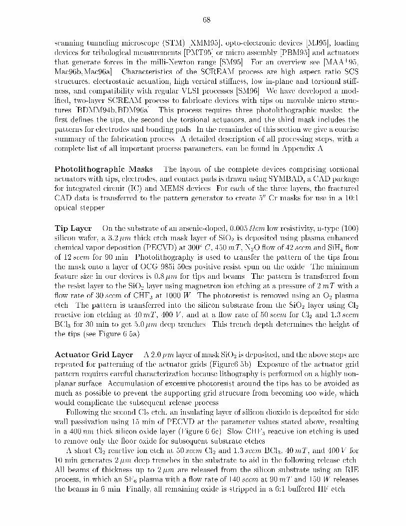
68

scanning tunneling microscope (STM) [XMM95], opto-electronic devices [MJ95], loadingdevices for tribological measurements [PMT95] or micro assembly [PBM95] and actuatorsthat generate forces in the milli-Newton range [SM95]. For an overview see [MAA+95,Mac96b,Mac96a]. Characteristics of the SCREAM process are high aspect ratio SCSstructures, electrostatic actuation, high vertical sti�ness, low in-plane and torsional sti�-ness, and compatibility with regular VLSI processes [SM96]. We have developed a mod-i�ed, two-layer SCREAM process to fabricate devices with tips on movable micro struc-tures [BDMM94b,BDM96a]. This process requires three photolithographic masks: the�rst de�nes the tips, the second the torsional actuators, and the third mask includes thepatterns for electrodes and bonding pads. In the remainder of this section we give a concisesummary of the fabrication process. A detailed description of all processing steps, with acomplete list of all important process parameters, can be found in Appendix A.

Photolithographic Masks. The layout of the complete devices comprising torsionalactuators with tips, electrodes, and contact pads is drawn using SYMBAD, a CAD packagefor integrated circuit (IC) and MEMS devices. For each of the three layers, the fracturedCAD data is transferred to the pattern generator to create 500 Cr masks for use in a 10:1optical stepper.

Tip Layer. On the substrate of an arsenic-doped, 0:005cm low resistivity, n-type (100)silicon wafer, a 3:2�m thick etch mask layer of SiO2 is deposited using plasma enhancedchemical vapor deposition (PECVD) at 300�C , 450mT , N2O ow of 42 sccm and SiH4 owof 12 sccm for 90 min. Photolithography is used to transfer the pattern of the tips fromthe mask onto a layer of OCG 985i 50cs positive resist spun on the oxide. The minimumfeature size in our devices is 0:8�m for tips and beams. The pattern is transferred fromthe resist layer to the SiO2 layer using magnetron ion etching at a pressure of 2mT with a ow rate of 30 sccm of CHF3 at 1000W . The photoresist is removed using an O2 plasmaetch. The pattern is transferred into the silicon substrate from the SiO2 layer using Cl2reactive ion etching at 40mT , 400V , and at a ow rate of 50 sccm for Cl2 and 1:3 sccmBCl3 for 30 min to get 5:0�m deep trenches. This trench depth determines the height ofthe tips (see Figure 6.5a).

Actuator Grid Layer. A 2:0�m layer of mask SiO2 is deposited, and the above steps arerepeated for patterning of the actuator grids (Figure6.5b). Exposure of the actuator gridpattern requires careful characterization because lithography is performed on a highly non-planar surface. Accumulation of excessive photoresist around the tips has to be avoided asmuch as possible to prevent the supporting grid structure from becoming too wide, whichwould complicate the subsequent release process.

Following the second Cl2 etch, an insulating layer of silicon dioxide is deposited for sidewall passivation using 15 min of PECVD at the parameter values stated above, resultingin a 400 nm thick silicon oxide layer (Figure 6.6c). Slow CHF3 reactive ion etching is usedto remove only the oor oxide for subsequent substrate etches.

A short Cl2 reactive ion etch at 50 sccm Cl2 and 1:3 sccm BCl3, 40mT , and 400V for10 min generates 2�m deep trenches in the substrate to aid in the following release etch.All beams of thickness up to 2�m are released from the silicon substrate using an RIEprocess, in which an SF6 plasma with a ow rate of 140 sccm at 90mT and 150W releasesthe beams in 6 min. Finally, all remaining oxide is stripped in a 6:1 bu�ered HF etch.

69

photoresistSi SiO2

tip

Tips

deep Si etch

pattern transfer

resist patterning

SiO2 deposition

(a)

Actuator Grids

deep Si etch

pattern transfer

resist patterning

SiO2 deposition

Si SiO2 photoresist

tip

gridactuator

(b)

Figure 6.5: Device fabrication with a two-layer SCREAM process: (a) forming of tipsusing an RIE chlorine etch, (b) fabrication of actuator structures consisting of SCS beamsof 1�m width.

70

SiO2Si

Release

sidewall SiO2

SiO2 trench etch

Si trench etch

release etch

(isotropic)

actuatorreleased

(c)

Si AlSiO2

Electrodes

dielectric SiO2

Al sputtering

Al patterning

(d)

Figure 6.6: Device fabrication with a two-layer SCREAM process: (c) MIE/RIE trenchbottom etch and RIE release etch, (d) Aluminum electrode deposition and patterning.

71

Electrode Layer. A 200 nm thin layer of dielectric PECVD silicon oxide is deposited. A250 nm layer of Al is conformally deposited using sputtering performed at 30mT pressure,with a beam current of 5A and an Ar ow rate of 30 sccm. Due to overhanging sidewalls(see Figure 6.6d) trench and mesa are electrically isolated. Note however that, because ofthe rather high degree of isotropy of the Al sputtering, the electrodes under the capacitorgrids consist of continuous Al. To pattern the Al in the trench we use lithography withOCG 985i 50cs positive resist. The pattern is transferred using Cl2 reactive ion etching at20mT , 400V , and ow rates of 20 sccm Cl2, 40 sccm BCl3, and 1:3 sccm CH4 for 1:5 min.

Finally, a 100 nm thick layer of PECVD SiO2 can be deposited on the device to avoidshorting when the actuators make contact with the trench electrodes during operation. Theactuators consist of beams that are close to 1�m wide and 5�m high, with approximately5�m clearance underneath. Our actuator designs have grids of 120� 240�m side length.The fabrication can be done in less than one week in the Cornell Nanofabrication Facility(CNF) at Cornell University.

Packaging and Testing. Chips of up to 6 cm � 2 cm with more than 3000 actuatorshave been packaged and wire-bonded. Larger arrays have been tested in the probe station.When an AC voltage (not necessarily at resonance frequency) is applied between the Alelectrodes and the Si substrate, the actuators are brought into an oscillatory motion. Thedielectric silicon oxide beween Al electrodes and Si substrate can withstand voltages of atleast 60V without breakdown.

6.1.3 Experimental Results

A wide variety of torsional resonators has been built and tested, yielding informationon the optimal design of actuators and material properties such as sti�ness, resonanceproperties, internal stresses, and energy dissipation. For a thorough discussion of torsionalresonators see [MZSM93,MM96]. In preliminary manipulation experiments, we dispensedcarbon particles of up to 10�m diameter on the actuator and observed the devices in theSEM. At resonance, the particles were quickly tossed o� the actuator.

Further manipulation experiments were performed on a prototype array with morethan 15,000 individual actuators. While the �rst generation of torsional resonators [MM96]exhibited only small de ections even at resonance, the current devices were designed forlarger displacements at DC voltages. This improvement was achieved by softer torsionalsprings and relatively larger capacitor grids (Figure 6.1). Out-of-plane motion of up to 5�m(the maximum kinematically possible de ection) was measured under the SEM. The �rstset of manipulation experiments was performed with small glass pieces (microscope coverslips) of a fewmm2 size and close to 1mg mass (note that the mass of an individual actuatormeasures less than 100 ng). We chose glass because it is at, rigid, and transparent,which makes it a favorable material to test our devices. However, because of its smoothsurface, the motion generated from the actuator array may be reduced because of slipbetween actuators and moving object. All manipulation experiments were performed inair. Therefore, damping and moisture on the hydrophilic surfaces of Aluminum and glassmay also reduce the e�ciency of the arrays.

We observed lifting of the glass pieces within the motion range of the actuators (sev-eral �m). The objects were also pushed sideways by several 100�m, by actuating thearray at about 50Hz for a few seconds, so that the actuators repeatedly struck the glass

72

Figure 6.7: Micro cilia device manipulating an ADXL50 accelerometer chip [Ana91] (cour-tesy of Dr. R. Payne, Analog Devices, Inc.); its size is 2:7mm squared. The SEM micro-graph shows a portion of the cilia chip, which consists of an 8� 8 array of motion pixels.The entire device includes four cilia chips that can be controlled independently to generatecomplex force vector �elds. Picture reproduced from [SGD+96].

piece. Larger distances were di�cult to achieve with the current arrays because of lowyield of our prototype devices. Depending on the shape of the object as well as its positionon the actuator array, we also observed resonance between actuators and object at certainactuation frequencies.

A second round of experiments was performed with pieces of paper. Paper is consider-ably rougher and lighter than a glass piece of equal size. With the current actuator arrayno motion could be observed. We believe that the main reason for this result is the highsurface roughness of paper which we measured as at least 10 - 100�m, which is more thanthe height of our current actuator tips, and larger than their range of motion. Low yieldin the current actuator arrays also reduces their e�ectiveness.

6.2 Polyimide Micro Cilia Arrays

We performed distributed manipulation experiments using an organic ciliary array of thin-�lm polyimide bimorph microactuators (Figure 6.7). These experiments constitute whatmay be the most convincing evidence to date in support of the theory of programmableforce �elds. The arrays were designed and built at the Center for Integrated Systems(CIS) at Stanford University by J. Suh, S. Glander, R. Darling, C. Storment, and G. Ko-vacs [SGD+96], who generously made them available to us, and collaborated with us duringour micro manipulation experiments. The actuators employ independent thermal actua-tion and electrostatic hold-down. Four orthogonally-oriented actuators are integrated intoa unit cell called a \motion pixel" [BDMM94b]. The motion pixels are replicated to tilea square area, allowing for precise manipulation of small objects placed on top of the

73

array. Our goal was to implement task-level, sensorless manipulation strategies for macro-scopic objects. The tasks of parts-translation, -rotation, -orientation, and -centering weredemonstrated using small IC dice. Strategies were programmed in a �ne-grained SIMD(Single Instruction Multiple Data) fashion by specifying planar force vector �elds. In ourexperiments, we employed vector �elds with potential for parts-orientation and -posingtasks, and the theory was used to predict the equilibrium poses of speci�c parts (Fig-ure 6.17). The poses predicted by the equilibrium analysis (see Section 2) were observedin our experiments (Figures 6.16-left).

Perhaps surprisingly, the theory has also predicted the existence of pathological �eldswhich do not induce well-behaved equilibria. In particular, the \lower bounds" of Section 3show that there exist perfectly plausible vector �elds which induce no stable equilibriumin very simple parts. Although these �elds are very simple, they result in limit cyclesand quite complex behavior. We implemented such �elds on the cilia array. Vector �eldswithout potential were employed to cast parts into limit cycles, e.g. \in�nite" rotation usinga skew-symmetric squeeze �eld. The predicted behavior (Figure 6.18) for such \unstable"vector �elds was also observed (Figure 6.16-right). This shows that rather complex|but potentially useful|behavior can be generated using very simple �elds. We believe ourexperiments validate the theory and suggest the practicality of such minimalist approachesto distributed manipulation.

The programmable vector �elds were implemented by actuating the organic cilia in acyclic, gait-like fashion. Motion in non-principal (e.g. diagonal) directions was e�ected bya pairwise coupling of the cilia to implement virtual cilia and virtual gaits, (analogous tothe virtual legs employed by Raibert's hopping and running robots [RHPR93]).

These experiments suggest that MEMS actuator arrays are useful for parts-orientation,-posing, -transfer, -singulation, and -sorting. Moreover, the theory of programmable vec-tor �elds and virtual gaits gives a method for controlling a very large number of distributedactuators in a principled, geometric, task-level fashion. Whereas many control theories formultiple independent actuators break down as the number of actuators becomes very large,our systems should only become more robust as the actuators become denser and morenumerous. This section represents a step towards testing that theory.

6.2.1 Devices and Experimental Setup

Several groups have described e�orts to apply MEMS (Micro Electro Mechanical System)actuators to component positioning, inspection, and assembly [PFH90,AOF93,Fuj93,BDMM94b,LW95, for example]. The Stanford cilia chip [SGD+96] employs independentthermal actuation and electrostatic hold-down of an array of 256 thin-�lm polyimide actu-ators (Figure 6.8) grouped together in 64 unit cells. Each cell consists of four orthogonally-oriented actuators called a \motion pixel" [BDMM94b], because it can generate motion invarious directions, spanning the plane. The motion pixels are replicated to tile a squarearea, allowing for precise manipulation of small objects placed on top of the array.

Combined Thermobimorph and Electrostatic Actuators. Surface micromachiningtechniques were used to create the actuators using polyimide as the primary structuralmaterial and aluminum as a sacri�cial layer. The fabrication process was designed to becompatible with CMOS or BiCMOS circuits which could be pre-fabricated on a siliconsubstrate.

74

Figure 6.8: Portion of a polyimide cilia array (SEM micrograph). Four orthogo-nally-oriented actuators are integrated into a motion pixel, which covers a surface areaof approximately 1:1� 1:1mm2. Picture reproduced from [SGD+96].

Each actuator cilium consists of two layers of polyimide with di�erent thermal expan-sion coe�cients. The cilium also contains a Titanium-Tungsten (Ti:W) resistive heaterloop for thermal actuation, Aluminum electrodes for electrostatic (low-power) hold-down,and a silicon nitride encapsulation/sti�ening layer (Figure 6.9).

Since the polyimides were cured at high temperature and the upper polyimide layerhas the larger thermal expansion coe�cient, the actuators assume an upward, out-of-planecurvature when the process is complete (Figure 6.10). Heating by the Ti:W resistorspartially attens them back towards the substrate. Then, applying a voltage between ciliaand substrate electrodes allows a low-power hold-down without heating current. For adetailed description of the fabrication process see [SGD+96].

Vertical and horizontal displacements of the cilia tips are a function of the thermalmismatch in the actuator layers. For room temperature, these values can be calculated as�v � 120�m and �h � 20�m [SGD+96]. Inspection under the scanning electron microscope(SEM) has veri�ed these calculations.

The lifting capacity of an actuator can be estimated as the force required to de ectthe actuator's tip to the substrate. The actuator load capacity has been calculated asFl = 76�N , which gives a force-per-area ratio of 4� 76�N =(1:1mm)2 � 250�N =mm2.

Chip Layout. The cilia array is composed of cells (motion pixels, each 1:1 � 1:1mm2)which contain four orthogonally-oriented actuators (Figure 6.10). On the current cilia chip,the motion pixels are arranged in an 8�8 array which occupies approximately 0:77 cm2 of a1 cm2 die. The four actuators of each pixel are independently activated by four thermal andfour electrostatic control lines. Within each column of eight cells, the thermal elements fora given actuator are wired in series, whereas the electrostatic elements for a given actuatororientation are wired in parallel. The eight columns are then wired in parallel for boththe thermal and electrostatic elements. Each electrostatic control line (E1 { E4) applies apotential to the electrodes of all 64 actuators of a given orientation. Similarly, each thermalcontrol line (T1 { T4) runs a current through the Ti:W heaters of all 64 actuators of a

75

(Curled out of plane when not heated)

Tip

TiW Resistor

High CTEPolyimide

Wet EtchAccessVias

ElectrostaticPlate

Low CTEPolyimide

Encapsulation/Stiffening Layer

Base

Figure 6.9: Organic thermal and electrostatic microactuator. Half of the upper polyimideand silicon nitride encapsulation/sti�ening layer are shown removed along the cilium's axisof symmetry to show details. Picture reproduced from [SGD+96].

given orientation, such that the load resistance for the overall array is the same as that ofa single element (� 1500). A common ground bus provides a current return path for thethermal elements, and a substrate contact provides an opposing plate for the electrostaticelements (Figure 6.11).

Four 8� 8 chips were diced and packaged together to make a quad-shaped 16� 16 ciliaarray device, with a total of 1024 cilia. The device itself is attached to a hybrid packagewhich is placed on a heat sink and thermo-electric cooler (Peltier e�ect module). Thetotal input power to the chip can exceed 4W , and without active cooling the packagecan become very hot. To observe the experiments, a long working-distance microscope isconnected to a CCD camera, and a video cassette recorder is used to monitor and recordboth the movements of an individual cilium and the objects conveyed by the array.

Controller. The manipulation results described below were accomplished with the ciliaarray device interfaced to an IBM 486 personal computer. The PC provides speed controlvia the drive pulse frequency and directional control interactively via keyboard or mouse,or by actuator programs that can be speci�ed using the MEMSA (MEMS Array) language1

which we developed at Stanford. The control software including the MEMSA interpreterwas written in PASCAL.

An 8-bit signal (4 electrostatic control lines E1 { E4, and 4 thermal control lines T1 {T4) is sent via the PC parallel port to D-type ip- ops which activate power transistors.Currently up to 4 cilia arrays can be controlled simultaneously by using a multiplexer with2 address bits. (Figure 6.12).

6.2.2 Low-level Control: Actuator Gaits

To induce motion on a part that is placed on the array, the cilia are actuated in a cyclic,gait-like fashion. In each cycle, the part is moved in a certain direction by the motion

1MEMSA (named after MENSA) is the language for smart manipulation surfaces.

76

Figure 6.10: Polyimide cilia motion pixel (SEM micrograph). Four actuators in a commoncenter con�guration make up a motion pixel. Each cilium is 430�m long and bends up to120�m out of the plane. Picture reproduced from [SGD+96].

of the actuators that are in contact with it. The speed of the moving part depends onthe (horizontal) displacement of the actuators per cycle as well as the frequency of cyclerepetition. It also depends on the surface properties and weight of the moving part.

Task: Translation of Parts in Principal Directions. The simplest gait is the two-phase gait, in which all actuators of the same orientation repeatedly stroke the part whilethe remaining actuators are held down. Assuming that the orthogonal cilia within a motionpixel are oriented at the principal compass points, let us use capital letters NEWS to denotethe North, East, West, and South actuators in the up position, and lower-case letters newsto denote the actuators in the lowered position. Then the two-phase gait to e�ect motionin the East direction would be news neWs (see Figure 6.13).

The four-phase gait consists of four di�erent actuation phases news neWs nEWs nEws

such that motion is induced during upward as well as downward strokes of the cilia (Fig-ure 6.14, see also [AOF93]). Note that the forces exerted on the moving part depend onthe state of the motion pixel: e.g. in the transition from phase 1 to phase 2 the cilium W

moves up while the opposing cilium e remains down. We denote the lateral force exertedon the part in this con�guration fW;e. Analogously, during transitions 2{3, 3{4, and 4{1we observe lateral forces fE;W, fw;E, and fe;w, respectively. fW;e and fe;w are in positive x-direction, while fE;W and fw;E are negative. Furthermore, from this analysis it follows thatjfW;ej � jfe;wj � jfE;Wj � jfw;Ej � 0. Hence we expect a relatively large motion step �xW;eduring transition 1{2, and a smaller step �xe;w during transition 4{1, while during theother transitions the part remains at its current location. This behavior has been observedin our experiments, where �xW;e was measured between 3�m and 10�m depending oninput power, frequency, surface properties and weight of the part. �xW;e was usually about

77

Electrostatic Interconnect Bus

GND

T1

T2

T3

T4

E1

E3

E4

E2

Ground Bus

Thermal Interconnect Bus

Figure 6.11: Polyimide cilia chip layout (not to scale), consisting of an 8�8 array of motionpixels with thermal and electrostatic control lines. Picture reproduced from [SGD+96].

twice as large as �xe;w.

Task: Translation of Parts in Arbitrary Directions. Motion in non-principal (e.g.diagonal) directions is e�ected by a pairwise coupling of two cilia of each pixel, implement-ing virtual cilia analogous to Raibert's concept of virtual legs for hopping and runningrobots [RHPR93]. Hence, several cilia can be coordinated to emulate a virtual cilium,which generates a force corresponding to the vector sum of its components. The diagonalgait to e�ect motion in the North-East direction would be news neWS NEWS NEws wherethe virtual cilia are NE and WS. Consequently, we obtain a virtual gait that moves thepart in a diagonal direction. Note that in a section view through the array looking in theNorth-West direction, this gait looks virtually identical to the four-phase gait depicted inFigure 6.14.

Motion in arbitrary directions can be induced by alternating gaits that interleave prin-cipal (and virtual) gaits of di�erent directions. For example, a translation at 25� from thex-axis requires motion in the y-direction and x-direction at a ratio of tan 25� � 1 : 2. Ourcontrol software determines the exact alternating sequence analogously to the Bresenhamline scan algorithm [FVDFH96], which rasterizes lines at arbitrary angles, resulting indi�erent �elds that are interlaced in time.

Experiments and Results. A large number of translation experiments have been per-formed in which two-phase and four-phase gaits were used to implement principal andvirtual gaits. These experiments show that a �rst-order dynamical system models the

78

E T E T E TE T

PC

MUX D D D Dclock

address

clock

data

parallel port

to power transistors and cilia chips

Figure 6.12: Schematic of cilia chip controller: eight data lines, two address lines, and oneclock line are used from the PC parallel interface. The data lines provide the activationpattern for the four electrostatic and the four thermal control lines of the cilia chip. Oneout of four cilia arrays is selected by the address via the multiplexer. New data is storedin the D-type ip- ops at every clock signal.

device-part interaction well. Therefore, when describing and predicting the motion of partsin force vector �elds, we have based our theory on a �rst-order system (see Section 6.2.3).

Silicon chips were moved with a motion resolution of a few �m and speeds up to200�m=sec. Four-phase gaits proved more e�ective than two-phase gaits, because dur-ing the downward motion in the two-phase gait, the part tends to slip backwards. Thefour-phase gait avoids this e�ect, because other cilia hold the part in place during thetransition 3{4. In the subsequent downward motion in the transition 4{1, the part is alsomoved forward (Figure 6.14).

The diagonal gait also has the lowest power consumption (not considering electrostatichold-down), due to the fact that its duty cycle for cilia hold-down is lowest (50%), com-pared to 75% for the principal four-phase gait, and 87.5% for the two-phase gait.

As expected, diagonal (virtual) gaits induced the largest and fastest motion because allfour cilia of each pixel were activated, whereas in principal gaits only two cilia are activelyused, while the others have to be held down continuously (Figure 6.14).

6.2.3 High-level Control: Vector Fields

We believe that vector �elds can be used as an abstraction barrier between applicationsrequiring array micro-manipulation and MEMS devices implementing the requisite me-chanical forces. That is, applications such as parts-feeding can be formulated in terms ofthe vector �elds required. This then serves as a speci�cation which the underlying MEMSdevice technology must deliver. Conversely, the capabilities of MEMS array technologiesfor actuation can be formulated in terms of the vector �elds they can implement. Forexample, limitations in force magnitude are naturally expressed in vector �eld terms, as\small" vector �elds. Restrictions in directional selectivity and magnitude control can alsobe manifested as restrictions on the vector �eld abstraction (resulting in discretization inorientation or modulus). This means that MEMS designers can potentially ignore certain

79

phase 2

up (off) down (on)

21

phase 1

news neWs

motion

motion

North

East

West

South

Figure 6.13: Two-phase gait. The W actuator is repeatedly switched on and o�, while theother actuators always remain on, resulting in a news neWs sequence.

details of the application process, and instead focus on matching the required vector �eldspeci�cation. Then, once the capabilities of MEMS actuator arrays were published asvector �elds and tolerances, an application designer could look in a catalog to choose adevice technology based on the �eld speci�cation it promises to implement. This wouldfree application engineers from needing to know much about process engineering, in thesame way that software and algorithm designers often abstract away from details of thehardware. Such an abstraction barrier could permit hierarchical design, and allow appli-cation designs with greater independence from the underlying device technology. At thesame time, abstraction barriers could allow MEMS array technologies to be designed si-multaneously with the (abstract) vector �eld control. This development pattern could besimilar to the concurrent design of VLSI processors with their compilers, as is common incomputer architecture.

In the remainder of this section, we give brief summaries of theoretical results (seeSections 2 { 5) and compare them to experiments that we performed with the micro ciliaarray device.

6.2.4 Squeeze Fields

In Section 2 we proposed a family of control strategies called squeeze �elds and a planningalgorithm for parts-orientation (see Figures 2.1 and 2.2).

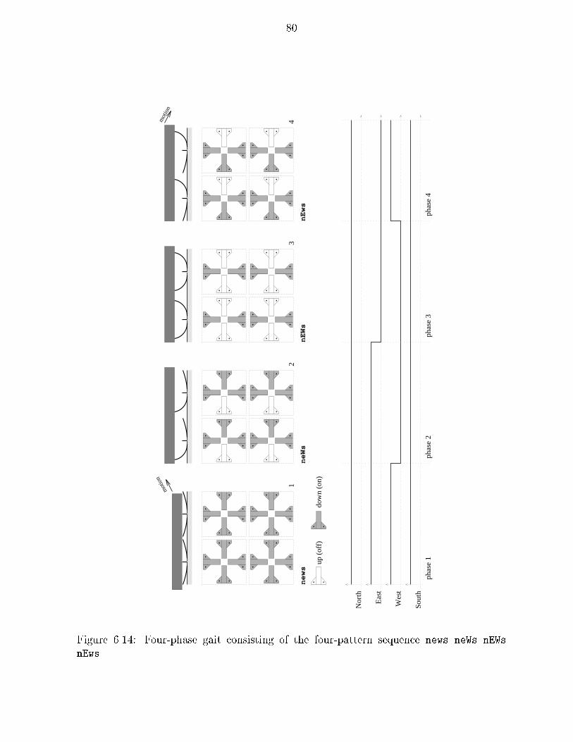
80

mot

ion

mot

ion

phas

e 1

phas

e 2

up (

off)

dow

n (o

n)

34

phas

e 3

phas

e 4

21

news

neWs

nEWs

nEws

Nor

th

Eas

t

Wes

t

Sou

th

Figure 6.14: Four-phase gait consisting of the four-pattern sequence news neWs nEWs

nEws.

81

mot

ion

mot

ion

phas

e 1

phas

e 2

up (

off)

dow

n (o

n)

phas

e 3

phas

e 4

12

34

news

neWS

NEWS

NEws

Nor

th

Sou

th

Wes

t

Eas

t

Figure 6.15: Diagonal (virtual) gait consisting of the four-pattern sequence news neWS

NEWS NEws. The N and E cilia, and the W and S cilia, are coupled to form virtual cilia inNorth-East and South-West directions.

82

Figure 6.16: Manipulation of silicon chips in programmable vector �elds induced by amicro cilia array (microscope video images).Left: The chip is aligned with the vertical squeeze line of the �eld.Right: Rotating a square-shaped chip counterclockwise in a skewed squeeze �eld. Picturesreproduced from [SGD+96].

83

Figure 6.17: Simulation of alignment task with a squeeze �eld.

De�nition 1 (Section 2.1) Assume l is a straight line through the origin. A squeeze�eld f is a two-dimensional force vector �eld de�ned as follows:

1. If z 2 R 2 lies on l then f(z) = 0.2. If z does not lie on l then f(z) is the unit vector normal to l and pointing towards l.

We refer to the line l as the squeeze line, because l lies in the center of the squeeze�eld.

Assuming quasi-static motion, an object will translate and rotate to an equilibriumcon�guration, as characterized in Figures 2.2, 2.3, and 2.4. This assumes a uniform forcedistribution over the surface of P , which is a reasonable assumption for a at part that isin contact with a large number of elastic actuators.

De�nition 2 (Section 2.1) A part P is in translational equilibrium if the forces actingon P are balanced. P is in orientational equilibrium if the moments acting on P arebalanced. Total equilibrium is simultaneous translational and orientational equilibrium.

Claim 42 [BDM96b] Every squeeze �eld f has potential, of the form U(z) =Z�f �

ds, where � is an arbitrary path to z from a �xed reference point. If dz denotes theperpendicular distance of z from the squeeze line, then U(dz) = jdzj.Proof: Follows from De�nition 1 and Proposition 17, Section 4. 2

Proposition 4 (Section 2.2) Let P be a polygon whose interior is connected. Thereexist O(k n2) bisectors such that P is in equilibrium when placed in a squeeze �eld suchthat the bisector coincides with the squeeze line. n is the part complexity measured asthe number of polygon vertices. k denotes the maximum number of polygon edges that abisector can cross.

If P is convex, then the number of bisectors is bounded by O(n).

Equilibria can be calculated analytically or numerically, see Section 2.2 for details.

Theorem 9 (Section 2.3) Let P be a polygon whose interior is connected. There existsan alignment strategy consisting of a sequence of squeeze �elds that uniquely orients P upto symmetries.

84

Figure 6.18: Unstable square-shaped part in a skewed squeeze �eld (� = �1). The squarewith center on the squeeze line will rotate inde�nitely. Moreover, it has no stable equilib-rium in this �eld.

Task: Orienting and Aligning Parts

If a part is placed in a squeeze �eld, it will translate and rotate until a stable equilibrium isreached (Proposition 4). Parts may exhibit several equilibria, hence after one squeeze thepart orientation may be ambiguous. This ambiguity can be removed with the strategies ofTheorem 9: by executing a sequence of squeezes at particular angles, the part is uniquelyoriented (see Figure 2.1, for details see Section 2.3).

Experiments and Results. The long, thin part depicted in Figures 6.16-left and 6.17exhibits a unique stable equilibrium (modulo 180� �eld symmetry). When placed in asqueeze �eld, its longitudinal axis aligns with the squeeze line. This dynamical process ispredicted by simulation in Figure 6.17, and veri�ed in experiment (see Figure 6.16-left).This part alignment experiment has also been performed with similar results for severalother small pieces of glass and silicon of a few mm length and several mg of mass.

6.2.5 Skewed Squeeze Fields

De�nition 11 (Section 3) A skewed �eld fS is a vector �eld given by fS(x; y) =�sign(x)(1; �), where 0 6= � 2 R .

Proposition 24 (Section 4.2) No skewed squeeze �eld has a potential.

Proposition 12 (Section 3) A skewed �eld induces no stable equilibrium on a disk-shaped part.

Proposition 13 (Section 3) A diagonally skewed �eld (� = �1) induces no stableequilibrium on a square-shaped part.

Task: Rotating Parts

According to Propositions 12 and 13, certain parts will rotate inde�nitely in skewed squeeze�elds (Figure 6.18). Note that even though our cilia device has more degrees of freedom,

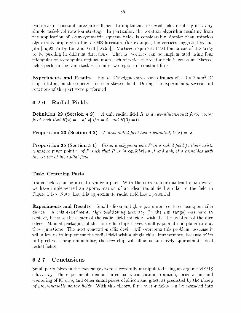
85

two areas of constant force are su�cient to implement a skewed �eld, resulting in a verysimple task-level rotation strategy. In particular, the rotation algorithm resulting fromthe application of skew-symmetric squeeze �elds is considerably simpler than rotationalgorithms proposed in the MEMS literature (for example, the vortices suggested by Fu-jita [Fuj93] or by Liu and Will [LW95]). Vortices require at least four areas of the arrayto be pushing in di�erent directions. That is, vortices can be implemented using fourtriangular or rectangular regions, upon each of which the vector �eld is constant. Skewed�elds perform the same task with only two regions of constant force.

Experiments and Results. Figure 6.16-right shows video frames of a 3 � 3mm2 ICchip rotating on the squeeze line of a skewed �eld. During the experiments, several fullrotations of the part were performed.

6.2.6 Radial Fields

De�nition 22 (Section 4.2) A unit radial �eld R is a two-dimensional force vector�eld such that R(z) = �z=jzj if z = 0, and R(0) = 0.

Proposition 23 (Section 4.2) A unit radial �eld has a potential, U(z) = jzj.

Proposition 35 (Section 5.1) Given a polygonal part P in a radial �eld f , there existsa unique pivot point v of P such that P is in equilibrium if and only if v coincides withthe center of the radial �eld.

Task: Centering Parts

Radial �elds can be used to center a part. With the current four-quadrant cilia device,we have implemented an approximation of an ideal radial �eld similar to the �eld inFigure 1.1-b. Note that this approximate radial �eld has a potential.

Experiments and Results. Small silicon and glass parts were centered using our ciliadevice. In this experiment, high positioning accuracy (in the �m range) was hard toachieve, because the center of the radial �eld coincides with the the location of the diceedges. Manual packaging of the four cilia chips leaves small gaps and non-planarities atthese junctions. The next generation cilia device will overcome this problem, because itwill allow us to implement the radial �eld with a single chip. Furthermore, because of itsfull pixel-wise programmability, the new chip will allow us to closely approximate idealradial �elds.

6.2.7 Conclusions

Small parts (sizes in the mm range) were successfully manipulated using an organic MEMScilia array. The experiments demonstrated parts-translation, -rotation, -orientation, and-centering of IC dice, and other small pieces of silicon and glass, as predicted by the theoryof programmable vector �elds. With this theory, force vector �elds can be cascaded into

86

OscillationsTransverse

PlateVibrating

Direction of Oscillation

Input Signal

Shaker

Figure 6.19: Schematic of experimental setup 1: A 50 cm�40 cm aluminum plate is forcedto oscillate horizontally by the shaker armature. The forced oscillation causes a transversevibration of the plate.

multi-step strategies. It has been shown that these open-loop strategies can sort as well asuniquely position and orient parts without sensor feedback.

Based on our experiments, a new, improved array is currently being fabricated. Bene�tsof the new, fully programmable cilia array will include among others the implementationof sequences of squeeze �elds, nearly-ideal radial �elds, and sensorless sorting strategies.The new design will also overcome current problems due to manual packaging.

6.3 Vibratory Plate Parts Feeders

In this section, we explore how controlled vibration can be used for a new device setupto systematically feed planar parts. The idea is to generate and change dynamic modesin a plate by varying applied frequencies. Depending on the frequency of vibration andthe boundary conditions, nodes of di�erent shapes are formed (this was experimentallystudied by Chladni [Chl87]). If planar parts are put on this vibrating plate, they move tothe node, and end up in a stable orientation [BBG95].

6.3.1 Setup and Calibration

Figures 6.19 and 6.20 are schematics of the experimental setup, which consists of an alu-minum plate forced to oscillate in two di�erent con�gurations. The shaker is a commer-cially available2 electrodynamic vibration generator, with a linear travel of 0:02m, andcapable of producing a force of up to 500N . The input signal, specifying the waveformcorresponding to the desired oscillations, is fed to a single coil armature, which moves ina constant �eld produced by a ceramic permanent magnet in a center gap con�guration.

In the �rst con�guration (Figure 6.19), the plate is attached to the shaker armature suchthat it is forced to vibrate in the longitudinal direction. For low amplitudes and frequen-cies, the plate moves longitudinally with no perceptible transverse vibrations. However,as the frequency of oscillations is increased, transverse vibrations of the plate becomemore pronounced. The resulting motion is similar to the forced transverse vibration of arectangular plate, clamped on one edge and free along the other three sides.

2Model VT-100G, Vibration Test Systems, Akron, OH, USA.

87

Vibrating PlateRod

Input Signal

Shaker

Oscillation

of Plate

Hinge

Osc

illat

ion

of a

rmat

ure

and

rod

Figure 6.20: Schematic of experimental setup 2: The aluminum plate is hinged and canoscillate about an axis in its middle.

The nodes for these transverse oscillations can either be obtained theoretically(Rayleigh [Ray45], Timoshenko [Tim40]), or experimentally using the technique originallypioneered by Chladni [Chl87]. By sprinkling small sized particles3 on a vibrating surface,the nodes can be experimentally identi�ed as the regions where the particles tend to col-lect. The dynamics of \collecting" at the nodes is important in determining the e�ectiveforce �eld that leads to the orienting and localization e�ect of our device, and is discussedin more detail in Section 6.3.3.

For the con�guration in Figure 6.19, the location and shape of the node depends onthe frequency of vibration. Figure 6.21 shows the experimental determination of the nodesfor frequencies of 60Hz and 100Hz .

The second con�guration (Figure 6.20) forces the plate to undergo transverse vibrationssuch that the resulting shape of the node, and its location, are independent of the forcingfrequency. The plate is hinged about an axis situated midway between, and parallel to,two of its sides. A rod connected to the armature of the shaker forces the plate to anoscillatory motion about the hinged axis. As expected, experimental determination showsthat except for a slight distortion due to the e�ect of clamping at the rod, the node linesup with the hinge axis (Figure 6.22).

The second setup is run at lower frequencies, to ensure that only the mode wherethe plate oscillates about the hinge axis is excited. If we increase the operating frequency,modes corresponding to transverse vibration of a plate, clamped at the point of attachmentto the rod and the hinged ends, become dominant, and the node shape gets complicated.This e�ect can be seen at 20Hz (Figure 6.22), where the node shows a tendency to get\pulled" towards the point where the plate is clamped to the rod.

6.3.2 Behavior of Planar Parts

3Chladni used sand, we use Urad lentils to get a better contrast on video.

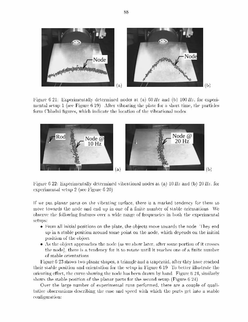
88

Node

(a)

Node

(b)

Figure 6.21: Experimentally determined nodes at (a) 60Hz and (b) 100Hz , for experi-mental setup 1 (see Figure 6.19). After vibrating the plate for a short time, the particlesform Chladni �gures, which indicate the location of the vibrational nodes.

Node @10 Hz

Rod

(a)

Node @20 Hz

(b)

Figure 6.22: Experimentally determined vibrational nodes at (a) 10Hz and (b) 20Hz , forexperimental setup 2 (see Figure 6.20).

If we put planar parts on the vibrating surface, there is a marked tendency for them tomove towards the node and end up in one of a �nite number of stable orientations. Weobserve the following features over a wide range of frequencies in both the experimentalsetups:

� From all initial positions on the plate, the objects move towards the node. They endup in a stable position around some point on the node, which depends on the initialposition of the object.

� As the object approaches the node (as we show later, after some portion of it crossesthe node), there is a tendency for it to rotate until it reaches one of a �nite numberof stable orientations.

Figure 6.23 shows two planar shapes, a triangle and a trapezoid, after they have reachedtheir stable position and orientation for the setup in Figure 6.19. To better illustrate theorienting e�ect, the curve showing the node has been drawn by hand. Figure 6.24, similarlyshows the stable position of the planar parts for the second setup (Figure 6.24).

Over the large number of experimental runs performed, there are a couple of quali-tative observations describing the ease and speed with which the parts get into a stablecon�guration:

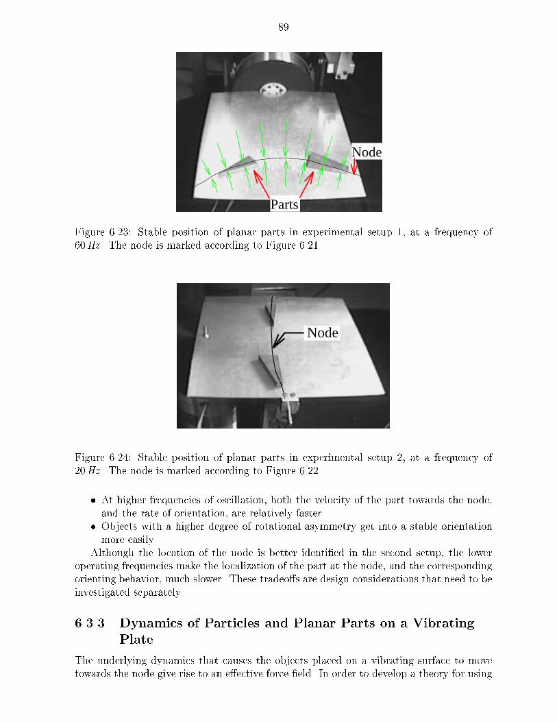
89

Parts

Node

Figure 6.23: Stable position of planar parts in experimental setup 1, at a frequency of60Hz . The node is marked according to Figure 6.21.

Node

Figure 6.24: Stable position of planar parts in experimental setup 2, at a frequency of20Hz . The node is marked according to Figure 6.22.

� At higher frequencies of oscillation, both the velocity of the part towards the node,and the rate of orientation, are relatively faster.

� Objects with a higher degree of rotational asymmetry get into a stable orientationmore easily.

Although the location of the node is better identi�ed in the second setup, the loweroperating frequencies make the localization of the part at the node, and the correspondingorienting behavior, much slower. These tradeo�s are design considerations that need to beinvestigated separately.

6.3.3 Dynamics of Particles and Planar Parts on a Vibrating

Plate

The underlying dynamics that causes the objects placed on a vibrating surface to movetowards the node give rise to an e�ective force �eld. In order to develop a theory for using

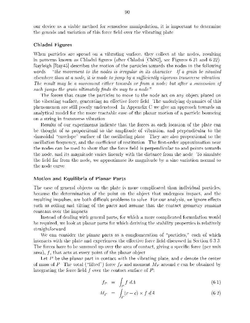
90

our device as a viable method for sensorless manipulation, it is important to determinethe genesis and variation of this force �eld over the vibrating plate.

Chladni Figures

When particles are spread on a vibrating surface, they collect at the nodes, resultingin patterns known as Chladni �gures (after Chladni [Chl87], see Figures 6.21 and 6.22).Rayleigh [Ray45] describes the motion of the particles towards the nodes in the followingwords { \the movement to the nodes is irregular in its character. If a grain be situatedelsewhere than at a node, it is made to jump by a su�ciently vigorous transverse vibration.The result may be a movement either towards or from a node; but after a succession ofsuch jumps the grain ultimately �nds its way to a node."

The forces that cause the particles to move to the node act on any object placed onthe vibrating surface, generating an e�ective force �eld. The underlying dynamics of thisphenomenon are still poorly understood. In Appendix C we give an approach towards ananalytical model for the more tractable case of the planar motion of a particle bouncingon a string in transverse vibration.

Results of our experiments indicate that the forces at each location of the plate canbe thought of as proportional to the amplitude of vibration, and perpendicular to thesinusoidal \envelope" surface of the oscillating plate. They are also proportional to theoscillation frequency, and the coe�cient of restitution. The �rst-order approximation nearthe nodes can be used to show that the force �eld is perpendicular to and points towardsthe node, and its magnitude varies linearly with the distance from the node. To simulatethe �eld far from the node, we approximate its magnitude by a sine variation normal tothe node curve.

Motion and Equilibria of Planar Parts

The case of general objects on the plate is more complicated than individual particles,because the determination of the point on the object that undergoes impact, and theresulting impulses, are both di�cult problems to solve. For our analysis, we ignore e�ectssuch as rolling and tilting of the parts and assume that the contact geometry remainsconstant over the impacts.

Instead of dealing with general parts, for which a more complicated formulation wouldbe required, we look at planar parts for which deriving the stability properties is relativelystraightforward.

We can consider the planar parts as a conglomeration of \particles," each of whichinteracts with the plate and experiences the e�ective force �eld discussed in Section 6.3.3.The forces have to be summed up over the area of contact, giving a speci�c force (per unitarea), f , that acts at every point of the planar object.

Let P be the planar part in contact with the vibrating plate, and c denote the centerof mass of P . The total (\lifted") force fP and moment MP around c can be obtained byintegrating the force �eld f over the contact surface of P :

fP =ZPf dA (6.1)

MP =ZP(r � c)� f dA (6.2)

91

Consider a part P on the vibrating plate. We assume that a �rst-order dynamicalsystem describes the motion of P on the plate. In a �rst-order system, the velocity of apart is directly proportional to the force acting on it. Hence, an equilibrium is a placementof P such that P remains stationary. In an equilibrium, the force and moment acting on Pare balanced. This equilibrium condition is met when the lifted force fP and moment MP

(Equations (6.1) and (6.2)) are both zero.We have made a series of assumptions to suggest that a force �eld exists for parts on a

planar plate. Our experimental results indicate that they are good engineering assumptionswhen we observe the system over time, due to an averaging e�ect caused by the vibrationof the plate. An \exact" modeling of the impact dynamics between part and plate, eventhough possible (see e.g. [MC95]), is not necessary for our purposes.

Chapter 7

Conclusions and Open Problems

7.1 Universal Feeder-Orienter (UFO) Devices

It was shown in Proposition 4 that every connected polygonal part P with n verticeshas a �nite number of stable orientation equilibria when P is placed into a squeeze �eldS. Based on this property we were able to generate manipulation strategies for uniquepart alignment. We showed in Section 5.1 that by using a combined radial and squeeze�eld R + �S, the number of equilibria can be reduced to O(k n). Using elliptic force�elds f(x; y) = (�x; �y) such that � 6= � and �; � 6= 0, this bound can be reduced totwo [Kav95,Kav97]. An \inertial" squeeze �eld f(x; y) = (�sign(x)x2; 0) uniquely orientsa part modulo �eld symmetry �. In a stable equilibrium, the part's major principal axisof inertia lines up with the squeeze line to minimize the second moment of inertia.

Does there exist a universal �eld that, for every part P , has only one unique equilibrium(up to part symmetry)? Such a �eld could be used to build a universal parts feeder [AE96]that uniquely positions a part without the need of a clock, sensors, or programming.

We propose a combined radial and \gravitational" �eld R+ �G which might have thisproperty. � is a small positive constant, and G is de�ned as G(x; y) = (0;�1). This devicedesign is inspired by the \universal gripper" in [AE96]. Such a �eld could be obtained froma MEMS array that implements a unit radial force �eld. Instead of rectangular actuators ina regular grid, triangular actuators could be laid out in a polar-coordinate grid. The arraycould then be tilted slightly to obtain the gravity component. Hence such a device wouldbe relatively easy to build. Alternatively, a resonating speaker, or a vibrating disk-shapedplate that is �xed at the center, might be used to create a radial force �eld. Extensivesimulations show that for every part we have tried, one unique total equilibrium is alwaysobtained. We are working toward a rigorous proof of this experimental observation.

7.2 Magnitude Control

Consider an array in which the magnitude of the actuator forces cannot be controlled.Does there exist an array with constant magnitude in which all parts reach one uniqueequilibrium? Or can one prove that, without magnitude control, the number of distinctequilibria is always greater than one?

92

93

7.3 Geometric Filters

This thesis focuses mainly on sensorless manipulation strategies for unique positioning ofparts. Another important application of programmable vector �elds are geometric �lters,which would be useful for sorting and singulation of parts. Figure 1.1 shows a simple �lterthat separates smaller and larger parts. We are interested in the question Given n parts,does there exist a vector �eld that will separate them into speci�c equivalence classes? Forexample, does there exist a �eld that moves small and large rectangles to the left, andtriangles to the right? In particular, it would be interesting to know whether for any twodi�erent parts there exists a sequence of force �elds that will separate them.

7.4 Force Field Computers

In this thesis we have demonstrated that even with a rather limited vocabulary of simpleforce �elds, useful and quite complex tasks such as sensorless posing or sorting of parts canbe performed. It might be possible that force �elds could be used to solve certain classesof problems, by encoding them in particular force �elds, part shapes, and initial and goalposes, resulting in a \force �eld computer" that provides a physical implementation of theproblem. Identifying the class of encodable problems might yield deeper insights into thecomplexity of parts manipulation with force vector �elds.

7.5 Performance Measures

Are there performance measures for how fast (in real time) an array will orient a part? Insome sense the actuators are �ghting each other (as we have observed experimentally) whenthe part approaches equilibrium. For squeeze grasps, one measure of \e�ciency," albeit

crude, might be the integral of the magnitude of the moment function, i.e.,Z 2�

0jM(�)j d�.

The issue is that if, for many poses, jM(�)j is very small, then the orientation process willbe slow. Better measures are also desirable.

7.6 Uncertainty

In practice, neither the force vector �eld nor the part geometry will be exact, and bothcan only be characterized up to tolerances [Don89]. This is particularly important atmicro scale. Within the framework of potential �elds, we can express this uncertaintyby considering not one single potential function UP , but rather families of potentials thatcorrespond to di�erent values within the uncertainty range. Bounds on part and forcetolerances will correspond to limits on the variation within these function families. Aninvestigation of these limits will allow us to obtain upper error bounds for manipulationtasks under which a speci�c strategy will still achieve its goal.

A family of potential functions is a set fU� : C ! Rg�2J where J is an index set. Forexample, we may start with a single potential function U : C ! R , and de�ne a familyof potential functions F(U; �; z) as fU� : C ! R j kU�(p) � U(p)kz < �g for some � andnorm z. This is analogous to de�ning a neighborhood in function space, using e.g. thecompact-open topology.

94

When we di�erentiate a family of potential �elds (using the gradient) we obtain adi�erential inclusion instead of a di�erential equation. So if F(u) = F(u; �; z), thenrF(u) = frU�g�2J .

When considering families of potentials, the equilibrium may be known to lie onlywithin a set Ei, although we may know that it is always a point in Ei. If the sets Ei areof a small diameter less than some � > 0, our algorithms could be extended to handle�-approximations.

As a more general approach, we propose an algorithm based on back-projections: For agiven part, let BFi(G) � C = R

2�S1 be the back-projection [LPMT84] of the set G underFi, where G � C, and Fi is a family of �elds on R 2. Then we wish to calculate a sequenceof �elds F1; F2; � � � ; Fk such that BF1(BF2(� � �BFk(G) � � �)) = C, where G is a single pointin C (cf. [LPMT84,EM88,Bro88,Don89,Bri92]).

7.7 Output Sensitivity

We have seen in Sections 2.1, 5.1, and 5.2 that the e�ciency of planning and executingmanipulation strategies critically depends on the number of equilibrium con�gurations.Expressing the planning and execution complexity as a function of the number of equilibriaE, rather than the number of vertices n, is called output sensitive analysis. In practice,we have found that there are almost no parts with more than two distinct (orientation)equilibria, even in squeeze �elds. This is far less than the E = O(k n2) upper boundderived in Section 2.2. If this observation can be supported by an exact or even statisticalanalysis of part shapes, it could lead to extremely good expected bounds on plan lengthand planning time, even for the less powerful strategies employing manipulation grammars(note that the complexity of the manipulation grammar algorithm in Proposition 41 isoutput-sensitive).

7.8 Discrete Force Fields

For the manipulation strategies described in this thesis we assume that the force �eldsare continuous, i.e. that the generated forces are dense compared to the moving part (as-sumption Density in Section 2.3). When manipulating very small parts on microactuatorarrays, this condition may be only approximately satis�ed. We are interested in the lim-itations of the continuous model, and we would like to know the conditions under whichit is necessary to employ a di�erent, discrete model of the array that takes into accountindividual actuators, as well as the gaps between actuators. In [BDMM94b] we propose amodel for the interaction between parts and arrays of individual actuators based on thetheory of limit surfaces [GR88,GRP91].

7.9 Resonance Properties

Is it possible to exploit the dynamic resonance properties of parts to tune the control signalof the array or plate to perform e�cient dynamic manipulation?

95

7.10 3D Force Fields

It may be possible to generate 3D force �elds by using Lorentz electromagnetic forces.Tunable electric coils could be attached to various points of a 3D body, suspending the re-sulting object in a strong permanent magnetic �eld using magnetic levitation (the Lorentze�ect) [HS93,SWH95]. The tuning (control) of the electric coils could be e�ected as fol-lows: Integrated control circuitry could be fabricated and co-located with the coils, andconceivably a power supply. The control could be globally e�ected using wireless commu-nication, or, the control of each coil evolves in time until the part is reoriented as desired.The Lorentz forces could then be deactivated to bring the object to rest on the ground.Planning for such a 3D device might reduce to [EMV93].

Appendix A

SCREAM Process

A.1 Processing Template

A.1.1 Photolithographic Masks

CAD

Symbad polygon editor, Dracula polygonfracturing1. generate design : : : : : : : : : : : : : : : : : : ped2. fracture design : : : : : : : : : : : : : : : symbpg3. check pattern : : : : : pgflash, pgcheck,

jebcad

4. transfer pattern to pattern generator :pgnet

=) �le: : : : : : : : : : : : : : : : : : : : :=) ashcount: : : : : : : : : : : : :

96

97

Pattern Generation

GCA Mann 3600 Pattern Generator1. load mask2. load data �le3. set parameters4. expose

) �le: : : : : : : : : : : : : : : : : : : : :) mask type: : : : : : : : : : : : :

=) mask name: : : : : : : : : : : :

Chrome Mask Making

1. MF320 develop : : : : : : : : : : : : : : : : 2 min2. DI rinse : : : : : : : : : : : : : : : : : : : : : : : 1 min3. DI soak : : : : : : : : : : : : : : : : : : : : : : : 2 min4. resist descum (O2 plasma)5. Chrome Etchant : : : : : : : : : : : : : 1.5 min6. DI rinse : : : : : : : : : : : : : : : : : : : : : : : 1 min7. DI soak : : : : : : : : : : : : : : : : : : : : : : : 2 min8. resist strip (1165 remover or O2

plasma)

) mask name: : : : : : : : : : : :

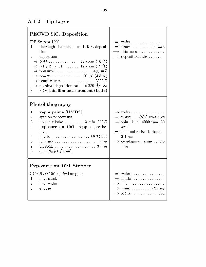
98

A.1.2 Tip Layer

PECVD SiO2 Deposition

IPE System 10001. thorough chamber clean before deposi-

tion2. deposition! N2O : : : : : : : : : : : : : : : : : 42 sccm (70 %)! SiH4 (Silane) : : : : : : : : 12 sccm (17 %)! pressure : : : : : : : : : : : : : : : : : : : : : 450 mT! power : : : : : : : : : : : : : : : : : 50 W (4.5 %)! temperature : : : : : : : : : : : : : : : : : : 300�C! nominal deposition rate � 380 �A/min

3. SiO2 thin �lm measurement (Leitz)

) wafer: : : : : : : : : : : : : : : : : :) time: : : : : : : : : : : : 90 min

=) thickness : : : : : : : : : : : : : : :=) deposition rate : : : : : : : :

Photolithography

1. vapor prime (HMDS)2. spin on photoresist3. hotplate bake : : : : : : : : : : 3 min, 90�C4. exposure on 10:1 stepper (see be-

low)5. develop : : : : : : : : : : : : : : : : : : : : OCG 9456. DI rinse : : : : : : : : : : : : : : : : : : : : : : : 1 min7. DI soak : : : : : : : : : : : : : : : : : : : : : : : 3 min8. dry (N2 jet / spin)

) wafer: : : : : : : : : : : : : : : : : :) resist: : : OCG 895i 50cs) spin, time 4000 rpm, 30

sec) nominal resist thickness

2.4 �m) development time : : 2.5

min

Exposure on 10:1 Stepper

GCA 6300 10:1 optical stepper1. load mask2. load wafer3. expose

) wafer: : : : : : : : : : : : : : : : : :) mask: : : : : : : : : : : : : : : : : :) �le: : : : : : : : : : : : : : : : : : : : :) time: : : : : : : : : : : 5.25 sec) focus: : : : : : : : : : : : : : 251

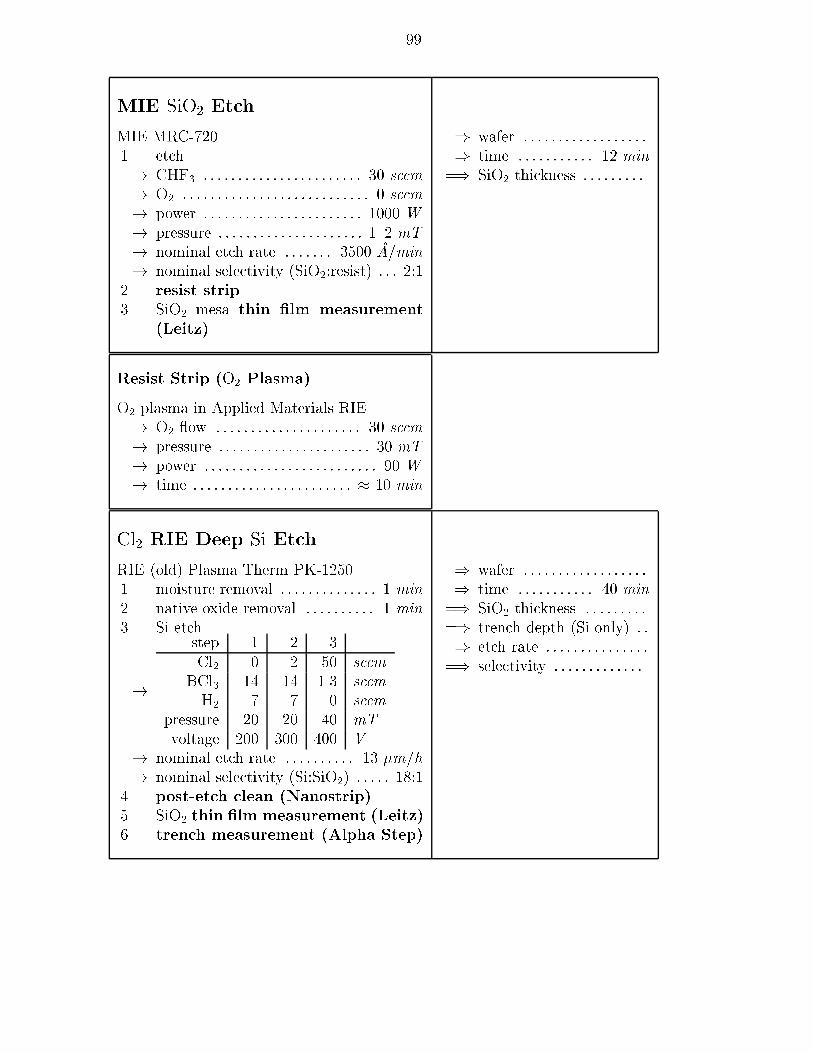
99

MIE SiO2 Etch

MIE MRC-7201. etch! CHF3 : : : : : : : : : : : : : : : : : : : : : : : 30 sccm! O2 : : : : : : : : : : : : : : : : : : : : : : : : : : : 0 sccm! power : : : : : : : : : : : : : : : : : : : : : : : 1000 W! pressure : : : : : : : : : : : : : : : : : : : : : 1{2 mT! nominal etch rate : : : : : : : 3500 �A/min! nominal selectivity (SiO2:resist) : : : 2:1

2. resist strip3. SiO2 mesa thin �lm measurement

(Leitz)

) wafer : : : : : : : : : : : : : : : : : :) time : : : : : : : : : : : 12 min

=) SiO2 thickness : : : : : : : : :

Resist Strip (O2 Plasma)

O2 plasma in Applied Materials RIE! O2 ow : : : : : : : : : : : : : : : : : : : : : 30 sccm! pressure : : : : : : : : : : : : : : : : : : : : : : 30 mT! power : : : : : : : : : : : : : : : : : : : : : : : : : 90 W! time : : : : : : : : : : : : : : : : : : : : : : : � 10 min

Cl2 RIE Deep Si Etch

RIE (old) Plasma Therm PK-12501. moisture removal : : : : : : : : : : : : : : 1 min2. native oxide removal : : : : : : : : : : 1 min3. Si etch

!

step 1 2 3Cl2 0 2 50 sccm

BCl3 14 14 1.3 sccmH2 7 7 0 sccm

pressure 20 20 40 mTvoltage 200 300 400 V

! nominal etch rate : : : : : : : : : : 13 �m=h! nominal selectivity (Si:SiO2) : : : : : 18:1

4. post-etch clean (Nanostrip)5. SiO2 thin �lm measurement (Leitz)6. trench measurement (Alpha Step)

) wafer : : : : : : : : : : : : : : : : : :) time : : : : : : : : : : : 40 min

=) SiO2 thickness : : : : : : : : :=) trench depth (Si only) : :=) etch rate : : : : : : : : : : : : : : :=) selectivity : : : : : : : : : : : : :

100

A.1.3 Actuator Grid Layer

PECVD SiO2 Deposition

IPE System 10001. thorough chamber clean before deposi-

tion2. deposition! N2O : : : : : : : : : : : : : : : : : 42 sccm (70 %)! SiH4 (Silane) : : : : : : : : 12 sccm (17 %)! pressure : : : : : : : : : : : : : : : : : : : : : 450 mT! power : : : : : : : : : : : : : : : : : 50 W (4.5 %)! temperature : : : : : : : : : : : : : : : : : : 300�C! nominal deposition rate � 380 �A/min

3. SiO2 thin �lm measurement (Leitz)

) wafer: : : : : : : : : : : : : : : : : :) time: : : : : : : : : : : : 40 min

=) thickness : : : : : : : : : : : : : : :=) deposition rate : : : : : : : :

Photolithography

1. vapor prime (HMDS)2. spin on photoresist3. hotplate bake : : : : : : : : : : 3 min, 90�C4. exposure on 10:1 stepper (see be-

low)5. develop : : : : : : : : : : : : : : : : : : : : OCG 9456. DI rinse : : : : : : : : : : : : : : : : : : : : : : : 1 min7. DI soak : : : : : : : : : : : : : : : : : : : : : : : 3 min8. dry (N2 jet / spin)

) wafer: : : : : : : : : : : : : : : : : :) resist: OCG 895i 16.5cs) spin, time 3000 rpm, 30

sec) nominal resist thickness

1.5 �m) development time : : 2.5

min

Exposure on 10:1 Stepper

GCA 6300 10:1 optical stepper1. load mask2. load wafer3. expose

) wafer: : : : : : : : : : : : : : : : : :) mask: : : : : : : : : : : : : : : : : :) �le: : : : : : : : : : : : : : : : : : : : :) time: : : : : 7.25 sec (non-

planar) / 4.75 sec (pla-nar)

) focus: : 284 (transparentmode)

101

MIE SiO2 Etch

MIE MRC-7201. etch! CHF3 : : : : : : : : : : : : : : : : : : : : : : : 30 sccm! O2 : : : : : : : : : : : : : : : : : : : : : : : : : : : 0 sccm! power : : : : : : : : : : : : : : : : : : : : : : : 1000 W! pressure : : : : : : : : : : : : : : : : : : : : : 1{2 mT! nominal etch rate : : : : : : : 3500 �A/min! nominal selectivity (SiO2:resist) : : : 2:1

2. resist strip3. SiO2 mesa thin �lm measurement

(Leitz)

) wafer : : : : : : : : : : : : : : : : : :) time : : : : : : : : : : : : : 5 min

=) SiO2 thickness : : : : : : : : :

Resist Strip (O2 Plasma)

O2 plasma in Applied Materials RIE! O2 ow : : : : : : : : : : : : : : : : : : : : : 30 sccm! pressure : : : : : : : : : : : : : : : : : : : : : : 30 mT! power : : : : : : : : : : : : : : : : : : : : : : : : : 90 W! time : : : : : : : : : : : : : : : : : : : : : : : � 10 min

Cl2 RIE Deep Si Etch

RIE (old) Plasma Therm PK-12501. moisture removal : : : : : : : : : : : : : : 1 min2. native oxide removal : : : : : : : : : : 1 min3. Si etch

!

step 1 2 3Cl2 0 2 50 sccm

BCl3 14 14 1.3 sccmH2 7 7 0 sccm

pressure 20 20 40 mTvoltage 200 300 400 V

! nominal etch rate : : : : : : : : : : 13 �m=h! nominal selectivity (Si:SiO2) : : : : : 18:1

4. post-etch clean (Nanostrip)5. SiO2 thin �lm measurement (Leitz)6. trench measurement (Alpha Step)

) wafer : : : : : : : : : : : : : : : : : :) time : : : : : : : : : : 37.5 min

=) SiO2 thickness : : : : : : : : :=) trench depth (Si only) : :=) etch rate : : : : : : : : : : : : : : :=) selectivity : : : : : : : : : : : : :

102

PECVD SiO2 Deposition

IPE System 10001. thorough chamber clean before deposi-

tion2. deposition! N2O : : : : : : : : : : : : : : : : : 42 sccm (70 %)! SiH4 (Silane) : : : : : : : : 12 sccm (17 %)! pressure : : : : : : : : : : : : : : : : : : : : : 450 mT! power : : : : : : : : : : : : : : : : : 50 W (4.5 %)! temperature : : : : : : : : : : : : : : : : : : 300�C! nominal deposition rate � 380 �A/min

3. SiO2 thin �lm measurement (Leitz)

) wafer: : : : : : : : : : : : : : : : : :) time: : : : : : : : : : : : 15 min

=) thickness : : : : : : : : : : : : : : :=) deposition rate : : : : : : : :

CHF3 RIE Trench Bottom Etch

(New) Plasma Therm System 721. CHF3 RIE : : : : : : : : : : : : : : : : : process 2! CHF3 : : : : : : : : : : : : : : : : : : : : : : : : : 100 %! O2 : : : : : : : : : : : : : : : : : : : : : : : : : : : : : : 2 %! pressure : : : : : : : : : : : : : : : : : : : : : : 40 mT! power (step 4) : : : : : : : : : : : : : : : : : 30 %! nominal etch rate : : : : : : : : 255 �A/min

2. SiO2 (mesa) thin �lm measurement(Leitz)

) wafer : : : : : : : : : : : : : : : : : :) time : : : : : : : : : : : 18 min

=) SiO2 thickness (mesa) : :=) etch rate : : : : : : : : : : : : : :

Cl2 RIE Deep Si Etch

RIE (old) Plasma Therm PK-12501. moisture removal : : : : : : : : : : : : : : 1 min2. native oxide removal : : : : : : : : : : 1 min3. Si etch

!

step 1 2 3Cl2 0 2 50 sccm

BCl3 14 14 1.3 sccmH2 7 7 0 sccm

pressure 20 20 40 mTvoltage 200 300 400 V

! nominal etch rate : : : : : : : : : : 13 �m=h! nominal selectivity (Si:SiO2) : : : : : 18:1

4. post-etch clean (Nanostrip)5. SiO2 thin �lm measurement (Leitz)6. trench measurement (Alpha Step)

) wafer : : : : : : : : : : : : : : : : : :) time : : : : : : : : : : : 10 min

=) SiO2 thickness : : : : : : : : :=) trench depth (Si only) : :=) etch rate : : : : : : : : : : : : : : :=) selectivity : : : : : : : : : : : : :

103

Release Etch

(New) Plasma Therm System 721. SF6 release etch : : : : : : : : : : : : process 5! SF6 : : : : : : : : : : : : : : : : : 140 sccm (70 %)! O2 : : : : : : : : : : : : : : : : : : : : : : : : : : : : : : 0 %! pressure : : : : : : : : : : : : : : : : : : : : : : 90 mT! power (step 4) : : : : : : : : : : : : : : : : : 30 %! nominal etch rate (isotropic) : : : : 1300

�A/min! nominal selectivity (Si:SiO2) 300:1

2. check release in SEM

) wafer : : : : : : : : : : : : : : : : : :) time : : : : : : : : : : : : : 6 min

=) etch rate : : : : : : : : : : : : : :

Oxide Strip (BHF)

1. BHF 6:1 soak : : : : : : : : : : : 15 { 30 min2. thorough rinse

A.1.4 Electrode Layer

PECVD SiO2 Deposition

IPE System 10001. thorough chamber clean before deposi-

tion2. deposition! N2O : : : : : : : : : : : : : : : : : 42 sccm (70 %)! SiH4 (Silane) : : : : : : : : 12 sccm (17 %)! pressure : : : : : : : : : : : : : : : : : : : : : 450 mT! power : : : : : : : : : : : : : : : : : 50 W (4.5 %)! temperature : : : : : : : : : : : : : : : : : : 300�C! nominal deposition rate � 380 �A/min

3. SiO2 thin �lm measurement (Leitz)

) wafer: : : : : : : : : : : : : : : : : :) time: : : : : : : : : : : 8.5 min

=) thickness : : : : : : : : : : : : : : :=) deposition rate : : : : : : : :

Sputter Deposition

CVC AST-601 Sputtering System! current : : : : : : : : : : : : : : : : : : : : : : DC 5 A! pressure : : : : : : : : : : : : : : : : : : : : : : 25 mT! Ar ow : : : : : : : : : : : : : : : : : : : : : 40 sccm! nominal deposition rate : : : : 90 �A/min

) wafer : : : : : : : : : : : : : : : : : :) ramp + presputter : 2 +

10 min) sputter time : : : : 28 min

=) thickness : : : : : : : : : : : : : :

104

Photolithography on Al

1. vapor prime (HMDS)2. spin on photoresist3. bake : : : : : : : : : : : : : : : : : : : 3 min, 90�C4. exposure on 10:1 stepper5. develop : : : : : : : : : : : : : MDC diluted 1:36. DI rinse : : : : : : : : : : : : : : : : : : : : : : : 1 min7. DI soak : : : : : : : : : : : : : : : : : : : : : : : 3 min8. dry (N2 jet / spin)

) wafer: : : : : : : : : : : : : : : : : :) resist: : : OCG 895i 50cs) spin, time 3000 rpm, 60

sec) nominal resist thickness

2.8 �m) development time 3 min

Exposure on 10:1 Stepper

GCA 6300 10:1 optical stepper1. load mask2. load wafer3. expose

) wafer: : : : : : : : : : : : : : : : : :) mask: : : : : : : : : : : : : : : : : :) �le: : : : : : : : : : : : : : : : : : : : :) time: : : : : 15.5 sec (non-

planar) / 12.5 sec (pla-nar)

) focus: : 284 (transparentmode)

Cl2 RIE Al Etch

RIE (old) Plasma Therm PK-1250

!

Cl2 20 sccmBCl3 40 sccmCH4 1.3 sccm

pressure 20 mTvoltage 400 V

! nominal etch rate : : : : : : : 2000 �A/min! nominal selectivity (Al:resist) : : : : : 2:1

) wafer : : : : : : : : : : : : : : : : : :) time : : : : : : : : : : 1:30 min

Resist Strip (O2 Plasma)

O2 plasma in Applied Materials RIE! O2 ow : : : : : : : : : : : : : : : : : : : : : 30 sccm! pressure : : : : : : : : : : : : : : : : : : : : : : 30 mT! power : : : : : : : : : : : : : : : : : : : : : : : : : 90 W! time : : : : : : : : : : : : : : : : : : : : : : : � 10 min

105

A.2 Processing Notes

Notes on CAD

� The pattern is fractured into rectangles. Therefore acute angles are not possible.However they are approximated to pattern generator resolution by a large numberof small (fractal-like) rectangles. Thus acute angles should be avoided.

� Fracturing is an NP-hard problem. Several heuristics are used which sometimes givenon-optimal or even surprising results.

� The order of the rectangles is optimized for pattern generator speed. Ordering prece-dence seems to be angle, size, location. pgcheck draws the rectangles in the order ofexposure.

� It is advantageous to have the origin of the mask exactly at the center. symbpg putsthe center at the exact geometric midpoint. Therefore the pattern should always bemade symmetric w.r.t. the origin.

� Standard alignment marks for the 10:1 stepper are generated with EXECUTE

cadmacros:gca key. Only necessary on the �rst mask. Make alignment marks astrenches, otherwise they may get released and disappear.

� ped library | CAD polygon editor.� symbpg (symbpg rev) | fracturing (with tone reversal). symbpg starts a batch job.The batch queue can be checked with show queue /batch.

� pgflash | print ashcounts and other information after fracturing.� pgcheck /d=gpx �le or jebcad | draw generated rectangles.� pg dump [/out=�le] | write rectangle �le in ASCII format.� pgmerge �le1,�le2,: : :,�leN out�le | merge rectangles of multiple �les.� (pgtape | write fractured pattern on tape for pattern generator.)� pgnet | transfer pattern to Pattern Generator

Notes on Pattern Generation

� Maximum �eld size is 10mm square with cut-o� corners. Largest full inscribedsquare is 9:4mm square.

� For chrome masks (shutter mode) approximately 7,000 to 8,000 ashes per hour.� Closure test produces pattern that is partially made before and after exposure. Thisway alignment shifts can be detected. Center rectangle is supposed to be exactlycentered. X:40 / Y:55 puts pattern in upper right corner. Avoid 55/55 because ofnon-uniform resist in corner, avoid 55/0 or 0/55 because of �ducials.

� Chrome masks (used here) have positive resist. Tone reversal is necessary to exposeeverything except pattern. Emulsion masks have negative resist.

� Mask needs �ducial marks (\C" for Cr masks) for alignment with the optical columnof the stepper.

� Only �rst mask needs CAD alignment marks.

Notes on Chrome Mask Making

� Chrome etch over light until chrome in exposed areas is gone, i.e. mask is clear.

106

Notes on PECVD SiO2 Deposition

� To avoid build-up of akes as much as possible, the chamber has to be very clean.Clean Process is often not su�cient. Remove all depositions inside the chamber.Remove shower head and scrub it in sink. Blow and vacuum chamber.

� Flakes tend to fall during and after chamber venting. Remove wafers as quickly aspossible and let them cool down outside chamber. Flakes falling down after processingcan mostly be removed with the N2 jet.

� Some users recommend short conditioning of chamber before deposition (a) to removeCF4 and (b) to bond loose particles left after clean (debatable).

� Some users suggest letting the system sit for a while after pumpdown at high tem-perature to get rid of moisture.

Notes on Photolithography

� HMDS vapor prime is preferred. Alternatively, bake wafer on 115�C hot plate for10 min to remove moisture. Cover whole wafer with HMDS 20 % and let sit for afew seconds. Then spin for 30 sec at 3000 rpm.

� Put a quarter-sized blob of resist on center of wafer before spinning, avoid bubblesas they may cause areas with no resist.

� Resist may be spread more evenly, and without the risk of leaving streaks of uncoatedwafer, if the spin speed is ramped up.

� Use chuck slightly smaller than wafer so that excess resist can get o� freely, avoidingedge beads.

� Resist (especially OCG 895i) does not stick well to Al (or rather Al2O3). ShipleySystem 8 sticks better. Very careful cleaning is necessary. It may be better to depositabout 1000 �A of SiO2 on Al for better adhesion. However, Al does not take PECVDtoo well, it tends to form bumps and bubbles.

� Re ectivity of Al causes focusing problem. Stepper can be switched to \transparent"mode.

� Most developers (especially OCG 945) attack Al. For lithography on Al use Microp-osit Developer Concentrate (MDC) diluted (1:3) with DI.

� Nominal resist thicknesses for OCG 895i (�m):rpm 3000 40005cs .8 .610cs 1.1 .9

16.5cs 1.5 1.322cs 1.7 1.534cs 2.1 1.950cs 2.8 2.4

� Some users recommend contrast enhancing material (CEM). CEM is opaque butbecomes transparent after a short exposure. It acts like an in-situ contact mask,improving resolution and sidewall slopes.

� Then, some users do not use BC5 but applies CEM365 directly to photoresist. Po-tential problem: CEM365 does not bond well to photoresist.

� AZ4903 thickness:

107

rpm �m750 30.01000 23.52000 14.63000 13.14000 10.75000 9.16000 8.07000 7.2

� Thick resist AZ4903 needs hold time (30 min) to absorb moisture before exposure.� Strip AZ4903 with AZ Thinner, AZ EBR, acetone, or O2 plasma.� 10x stepper delivers 58.08 mW =cm2.

Notes on Exposure on 10:1 Stepper

� Don't forget to get lamp into position after aligning mask.� Check shutters, opaque/transparent switch.� Exposure wavelength 365 nm.� For optimal alignment after loading or switching wafers and masks, wait at least 5min for temperature to settle inside the Stepper.

� Standard alignment marks are 63.5 mm apart.� Positions and spacing can be controlled with 5 digits accuracy.� To get standard alignment marks, spacing should be a divisor of 63.5 mm.� If an exposure has multiple passes, masks can be switched after each pass withoutlosing alignment.

� If parts of the exposure need di�erent masks, use multiple passes and useARRAY-DROPOUT to remove single dies from the exposure, or PLUG-PLUG IN to putsingle dies into the exposure. PLUG IN also allows an arbitrary o�set, so the die canbasically go anywhere.

� Syntax: EXEC <file>, PASS1, PASS2. After each pass the system waits and asksCHANGE RETICLES? Then replace masks.

� Masks have 4 �ducial marks, so they can be used in 4 orientations.� Exposure of dies is done as shown by ASCII-graphics on screen, but each individualdie is rotated by 180� due to the projection.

Notes on MIE SiO2 etch

� Etch is uniform up to about 1/2 inch to edge of wafer, where it is slower and verynonuniform. Therefore patterns close to the edge should be avoided. They willproduce a lot of grass.

� Watch the He pressure. If it drops, liquid He is leaking. This means the wafer willnot be cooled properly, and the He may mess up the etch.

� After chamber has been opened, always run chamber clean (O2 or CHF3) until pres-sure reaches � 5 mT .

Notes on Cl2 RIE Deep Si Etch

� If previous user did not etch Si (especially Al) make sure chamber is clean.

108

� Steps 1 and 2 may not be absolutely necessary.� Low Cl2 ow in Step 2 is hard to achieve. Start at higher ow and lower it gradually.Still, 2 sccm may not be stable.

Notes on CHF3 RIE Trench Bottom Etch

� Slow SiO2 etch for very thin �lms.� Make sure gas selector switch is on correct setting.� Watch DC bias voltage. Change in bias indicates build-up of polymers.

Notes on Release Etch

� Make sure gas selector switch is on correct setting.� Etch is rather non-uniform.� Some users recommend a short pre-release etch to get rid of oxide and other deposits:process 8, pressure 10 mT , power 15 %, CF4 50 %, O2 2 %.

� Some users use O2 chamber clean before release. Don't! Plasma Therm sta� recom-mends anything except O2 (in particular SF6) for chamber conditioning before releaseetch.

Notes on Sputter Deposition

� System takes long time to pump down.� Use monitor wafer to measure thickness, e.g. with partial resist for acetone lift-o�and alpha-step (usually provided by sta�).

� To close shutter, black nob must be in target sector.� Al with low percentage of Si supposedly has better properties for wire bonding, butis not very popular in the CNF.

� Breakdown voltage for PECVD SiO2 is about 300 V =�m. However voltage may leakthrough defects in oxide. Devices with leaks may still function as the leaks are rathersmall.

� Leaks and breakdown decrease with thicker �lms, but �lm stress increases, which inturn can cause leakage and breakdown.

Appendix B

Microscopic Model For Actuator

Contact

In this section we develop a model for the mechanics of microactuators. We make use oflimit surfaces [GR88] that describe anisotropic frictional contact. We extend the modelto active contacts and describe fast algorithms to compute the combined e�ect of manyactuators.Limit Surfaces. Assume we have a part P that moves on top of the actuator array. Thelimit surface L in load space (forces Fx and Fy, momentM) fully describes the relationshipbetween generalized velocity v, e�ective applied load Fe� , and frictional load Fr of the mov-ing part. It is based on the Maximum Work Inequality which is an engineering assumptioncommonly used when modeling friction or plasticity [GR88,PS88]. The Maximum WorkInequality generalizes Coulomb's friction law to anisotropic rate-independent friction. Thefollowing properties of limit surfaces are useful [GR88]:

1. L is a closed convex surface in load space.2. L contains all possible frictional loads Fr on P .3. If v 6= 0, Fr 2 L and �v is normal to L at Fr.4. Fr is the vector inside or on L such that the length of Fr � Fe� is minimal.5. In the special case when the moment component M of Fr is 0, L is a limit curve in

(Fx � Fy) load space.

FrFr

{v

{v

(a) (b)

Fy

Fx

Fy

Fx

Figure B.1: Limit curves: (a) �v is always normal to L at Fr. (b) Fr can be nonunique fora speci�c given v.

109

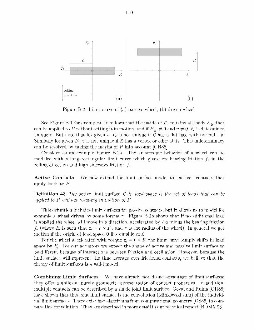
110

(a) (b)

rolling

direction

Fy

Fx

Fy

Fx

Fafs

fb

Figure B.2: Limit curve of (a) passive wheel, (b) driven wheel.

See Figure B.1 for examples. It follows that the inside of L contains all loads Fe� thatcan be applied to P without setting it in motion, and if Fe� 6= 0 and v 6= 0, Fr is determineduniquely. But note that for given v, Fr is not unique if L has a at face with normal �v.Similarly for given Fr, v is not unique if L has a vertex or edge at Fr. This indeterminacycan be resolved by taking the inertia of P into account [GR88].

Consider as an example Figure B.2a. The anisotropic behavior of a wheel can bemodeled with a long rectangular limit curve which gives low bearing friction fb in therolling direction and high sideways friction fs.

Active Contacts. We now extend the limit surface model to \active" contacts thatapply loads to P .

De�nition 43 The active limit surface L in load space is the set of loads that can beapplied to P without resulting in motion of P .

This de�nition includes limit surfaces for passive contacts, but it allows us to model forexample a wheel driven by some torque �a. Figure B.2b shows that if no additional loadis applied the wheel will move in y direction, accelerated by Fa minus the bearing frictionfb (where Fa is such that �a = r � Fa, and r is the radius of the wheel). In general we getmotion if the origin of load space 0 lies outside of L.

For the wheel accelerated with torque �a = r � Fa the limit curve simply shifts in loadspace by Fa. For our actuators we expect the shape of active and passive limit surface tobe di�erent because of interactions between friction and oscillation. However, because thelimit surface will represent the time average over frictional contacts, we believe that thetheory of limit surfaces is a valid model.

Combining Limit Surfaces. We have already noted one advantage of limit surfaces:they o�er a uniform, purely geometric representation of contact properties. In addition,multiple contacts can be described by a single joint limit surface. Goyal and Ruina [GR88]have shown that this joint limit surface is the convolution (Minkowski sum) of the individ-ual limit surfaces. There exist fast algorithms from computational geometry [GS88] to com-pute this convolution. They are described in more detail in our technical report [BDMM93].

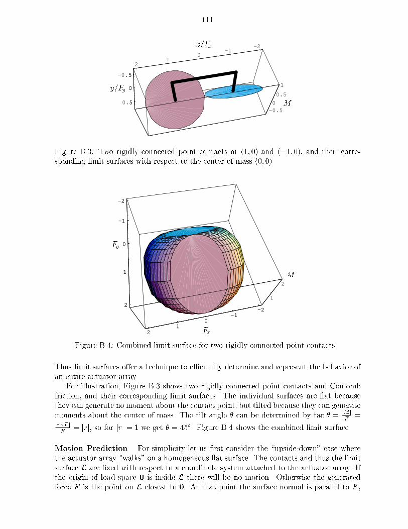
111

-2-1

01

2

-0.5

0

0.5

-0.50

0.5

1

5

0

5 M

x=Fx

y=Fy

Figure B.3: Two rigidly connected point contacts at (1; 0) and (�1; 0), and their corre-sponding limit surfaces with respect to the center of mass (0; 0).

-2-1

01

2

-2

-1

0

1

21

2

-2-1

01

2

2

1

0

1

2

M

Fx

Fy

Figure B.4: Combined limit surface for two rigidly connected point contacts.

Thus limit surfaces o�er a technique to e�ciently determine and represent the behavior ofan entire actuator array.

For illustration, Figure B.3 shows two rigidly connected point contacts and Coulombfriction, and their corresponding limit surfaces. The individual surfaces are at becausethey can generate no moment about the contact point, but tilted because they can generatemoments about the center of mass. The tilt angle � can be determined by tan � = jM j

jF j=

jr�F jjF j

= jrj, so for jrj = 1 we get � = 45�. Figure B.4 shows the combined limit surface.

Motion Prediction. For simplicity let us �rst consider the \upside-down" case wherethe actuator array \walks" on a homogeneous at surface. The contacts and thus the limitsurface L are �xed with respect to a coordinate system attached to the actuator array. Ifthe origin of load space 0 is inside L there will be no motion. Otherwise the generatedforce F is the point on L closest to 0. At that point the surface normal is parallel to F ,

112

so velocity and accelerating force are parallel. The walker will move on a straight line ora circle. This is not unexpected for a �xed actuator strategy on a homogeneous surface.

Now consider the case where the object is on top of the actuator array. There aretwo major di�erences to the previous case: When the object moves (1) some actuatorslose contact, others make contact, (2) the induced moment changes. (1) requires periodicupdates of the limit surface. (2) results in stretching of the limit surface along the momentaxis. Our technical report [BDMM93] gives details on how to handle these cases e�ciently.There, we outline a simple yet e�cient motion prediction algorithm: Numerically integratethe velocities computed as described above, and update the limit surface L accordingly.Each integration step can be done in constant time. Each update of L is linear in thecomplexity of L.

Motion Planning. The shape of the limit surface is determined by the activation pat-tern of the actuator array, which depends on each individual actuator. The limit surfacegives us a geometric representation of the forces and velocities generated with a speci�cactuator activation pattern. Though theoretically possible, there are practical limitationson using limit surfaces to plan microscopic manipulation strategies due to the combina-torial complexity and mechanical uncertainty. However, the microscopic model will proveimportant to analyze and verify strategies before fabrication. It forms the link between \ac-tuator macros" (Section 2.3) that predict the global behavior of manipulation strategies,and individual microfabricated mechanisms (Sections 6.1 and 6.2).

Appendix C

Particle Bouncing on a Vibrating

String

To understand the e�ective forces on particles on a vibrating surface, we look at themore tractable case of the planar motion of a particle bouncing on a string in transversevibrations (Figure C.1).

The string vibrates in the �rst mode, and is not a�ected by its interaction with theparticle. The shape of the string, at time t, for a given x location is:

ys = A sinx sin 2��t

where � is the frequency of oscillation. The position of the particle is given by (xp; yp).The interaction between the particle and the string is through a sequence of impacts.

We use a model for particle impact with a �nite friction coe�cient �, and a coe�cient ofrestitution e. � is the slope of the string at the point and instant of impact, and is smallfor small amplitudes of string vibration.

tan � = A cos x sin 2��t

The motion of the particle can be simulated as a series of impacts with the string, withthe particle in free ight in-between. The change in the momentum of the particle duringimpact is calculated using a simple planar impact model. Figure C.2 shows the results ofa numerical simulation of the model at two di�erent values of e.

y

�

ys = A sinx sin 2��t

n

t

A

(xp; yp)

x

�

Figure C.1: Particle bouncing on a vibrating string.

113

114

0 200 400 600 8000.1

0.2

0.3

0.4

0.5

0.6

0.7

0.8

timex

coor

dina

te

Low coeff of restitution, e = 0.1

0 100 200 300

0

0.2

0.4

0.6

0.8

1

1.2

1.4

1.6

time

x co

ordi

nate

High coeff of restitution, e = 0.9

Figure C.2: Simulation results showing the position of a particle moving on a vibratingstring.

For a particle starting at rest, at t = 0, we �nd that _yp � _xp. Using the assumptionthat the amplitude of oscillations is small, sin � � tan � ; cos � � 1. If ( _x�p ; _y

�p ) represent

the velocity just before impact, the velocity just after impact ( _x+p ; _y+p ), is:

_x+p = e ( _y�p � _y�s ) sin � + � v�relt (C.1)

_y+p = _y�s (1 + e)� e _y�p (C.2)

where v�relt = ( _y�p � _y�s ) sin � + _x�p is the relative velocity along the tangential directionbefore impact, and � 2 [0; 1] is the dissipation factor that depends on �.

After the impact, _x+p is a sum of the relative tangential velocity before impact, at-tenuated by friction; and a component from the impulse in the normal direction, whichdepends on e and the slope of the string at the point of impact. The portion of x impulseadded purely due to the e�ect of the string can be approximated as �e _ys sin �, by setting_y�p = 0.

If this component of the impulse were spread uniformly over time, the e�ective force,Fe� , that the particle would experience is:

Fe� / ��eA2 sinx cos 2��t cos x sin 2��t (C.3)

115

We now use the argument that it is more probable for the particle to impact the stringat times when the string is above the mean rest position, to show that over a large numberof impacts, the time dependent terms in equation (C.3) average out to a positive quantity.Therefore, the time averaged e�ective force, Favg , experienced by the particle is:

Favg / ��eA2 sin 2x

This con�rms the intuition and the observed behavior that the particle moves faster athigher amplitudes of string oscillation, coe�cient of restitution, and oscillation frequency.The sine dependency of the force with x ensures that it points towards the correspondingnodes on either side of the anti-node at x = �

2.

Bibliography

[AE96] Tamara Lynn Abell and Mike Erdmann. A universal parts feeder, 1996.Personal communication / in preparation.

[AHLM95] Srinivas Akella, Wesley H. Huang, Kevin M. Lynch, and Matthew T. Mason.Planar manipulation on a conveyor by a one joint robot with and withoutsensing. In International Symposium of Robotics Research (ISRR), 1995.

[Ana91] Analog Devices, Inc., Norwood, MA 02062. Introducing the ADXL50 Micro-machined Accelerometer Sensor, 1991.

[AOF93] Manabu Ataka, Akito Omodaka, and Hiroyuki Fujita. A biomimetic micromotion system. In Transducers | Digest Int. Conf. on Solid-State Sensorsand Actuators, pages 38{41, Paci�co, Yokohama, Japan, June 1993.

[BBD+95] Karl-Friedrich B�ohringer, Russell G. Brown, Bruce R. Donald, James S. Jen-nings, and Daniela Rus. Distributed robotic manipulation: Experiments inminimalism. In Fourth International Symposium on Experimental Robotics(ISER), Stanford, California, June 1995. http://www.cs.cornell.edu

/home/brd.

[BBG95] Karl-Friedrich B�ohringer, Vivek Bhatt, and Kenneth Y. Goldberg. Sensorlessmanipulation using transverse vibrations of a plate. In Proc. IEEE Int. Conf.on Robotics and Automation (ICRA), pages 1989 { 1996, Nagoya, Japan, May1995. http://www.cs.cornell.edu/home/karl/VibratoryAlign.

[BDH97] Karl-Friedrich B�ohringer, Bruce R. Donald, and Dan Halperin. The areabisectors of a polygon and force equilibria in programmable vector �elds. In13th ACM Symposium on Computational Geometry, Nice, France, June 1997.

[BDM96a] Karl-Friedrich B�ohringer, Bruce R. Donald, and Noel C. MacDonald. Single-crystal silicon actuator arrays for micro manipulation tasks. In Proc.IEEE Workshop on Micro Electro Mechanical Systems (MEMS), pages 7{12, San Diego, CA, February 1996. http://www.cs.cornell.edu/home

/karl/MicroActuators.

[BDM96b] Karl-Friedrich B�ohringer, Bruce R. Donald, and Noel C. MacDonald. Upperand lower bounds for programmable vector �elds with applications to MEMSand vibratory plate parts feeders. In International Workshop on Algorith-mic Foundations of Robotics (WAFR), Toulouse, France, July 1996. http:

//www.cs.cornell.edu/home/karl/MicroManipulation.

116

117

[BDMM93] Karl-Friedrich B�ohringer, Bruce R. Donald, Robert Mihailovich, and Noel C.MacDonald. A geometric theory of manipulation and control for micro-fabricated actuator arrays. Technical Report 93{87, Cornell University,Mathematical Sciences Institute, Ithaca, NY 14853, November 1993. http://www.cs.cornell.edu/home/karl/MicroActuators.

[BDMM94a] Karl-Friedrich B�ohringer, Bruce R. Donald, Robert Mihailovich, and Noel C.MacDonald. Sensorless manipulation using massively parallel microfabri-cated actuator arrays. In Proc. IEEE Int. Conf. on Robotics and Automa-tion (ICRA), pages 826{833, San Diego, CA, May 1994. http://www.cs

.cornell.edu/home/karl/MicroManipulation.

[BDMM94b] Karl-Friedrich B�ohringer, Bruce R. Donald, Robert Mihailovich, and Noel C.MacDonald. A theory of manipulation and control for microfabricated ac-tuator arrays. In Proc. IEEE Workshop on Micro Electro Mechanical Sys-tems (MEMS), pages 102{107, Oiso, Japan, January 1994. http://www.cs

.cornell.edu/home/karl/MicroActuators.

[BPM82] Geo�rey Boothroyd, Corrado Poli, and Laurence E. Murch. Automatic As-sembly. Marcel Dekker, Inc., 1982.

[Bri92] Amy J. Briggs. An e�cient algorithm for one-step planar compliant motionplanning with uncertainty. Algorithmica, 8(3), 1992.

[Bro86] Rod Brooks. A layered intelligent control system for a mobile robot. IEEEJournal of Robotics and Automation, RA(2), 1986.

[Bro88] Randy C. Brost. Automatic grasp planning in the presence of uncertainty.Int. Journal of Robotics Research, 7(1):3{17, 1988.

[CG94] John Canny and Ken Goldberg. \RISC" for industrial robotics: Recentresults and open problems. In Proc. IEEE Int. Conf. on Robotics and Au-tomation (ICRA). IEEE, May 1994.

[Chl87] Ernst Florens Chladni. Entdeckungen �uber die Theorie des Klanges. Weid-manns Erben und Reich, Leipzig, 1787.

[DJR95] Bruce Randall Donald, James Jennings, and Daniela Rus. Information in-variants for distributed manipulation. In K. Goldberg, D. Halperin, J.-C.Latombe, and R. Wilson, editors, International Workshop on AlgorithmicFoundations of Robotics (WAFR), pages 431{459, Wellesley, MA, 1995. A.K. Peters.

[DO90] M. D��az and J. O'Rourke. Ham-sandwich sectioning of polygons. In Proc.2nd Canadian Conference on Computational Geometry, pages 98{101, Ot-tawa, 1990.

[Don89] Bruce R. Donald. Error Detection and Recovery in Robotics, volume 336 ofLecture Notes in Computer Science. Springer Verlag, Berlin, 1989.

[Don90] Bruce R. Donald. The complexity of planar compliant motion planning withuncertainty. Algorithmica, 5(3):353{382, 1990.

118

[DX95] Bruce Randall Donald and Pat Xavier. Provably good approximation algo-rithms for optimal kinodynamic planning for cartesian robots and open chainmanipulators. Algorithmica, 14(6):480{530, November 1995.

[EM88] Michael A. Erdmann and Matthew T. Mason. An exploration of sensorlessmanipulation. IEEE Journal of Robotics and Automation, 4(4), August 1988.

[EM96] Michael A. Erdmann and Matthew T. Mason. Nonprehensile manipulation.In International Workshop on Algorithmic Foundations of Robotics (WAFR),Toulouse, France, July 1996.

[EMV93] Michael A. Erdmann, Matthew T. Mason, and G. Vane�cek, Jr. Mechanicalparts orienting: The case of a polyhedron on a table. Algorithmica, 10, 1993.

[Erd94] M. A. Erdmann. On a representation of friction in con�guration space. Int.Journal of Robotics Research, 13(3):240{271, 1994.

[Erd96] Michael A. Erdmann. An exploration of nonprehensile two-palm manipula-tion: Planning and execution. Technical report, Carnegie Mellon University,Pittsburgh, PA, 1996.

[FD86] Gregory T. Farnum and Bill Davis. Delivering the part. ManufacturingEngineering, March 1986.

[FHF91] T. Furuhata, T. Hirano, and H. Fujita. Array-driven ultrasonic microac-tuators. In Transducers | Digest Int. Conf. on Solid-State Sensors andActuators, pages 1056{1059, Montreux, France, June 1991.

[Fuj93] Hiroyuki Fujita. Group work of microactuators. In International AdvancedRobot Program Workshop on Micromachine Technologies and Systems, pages24{31, Tokyo, Japan, October 1993.

[FVDFH96] J. D. Foley, A. Van Dam, Feiner, and Hughes. Computer Graphics: Princi-ples and Practice. Addison Wesley, 2 edition, 1996.

[Gab95] Kaigham J. Gabriel. Engineering microscopic machines. Scienti�c American,273(3), September 1995.

[Gil56] Thomas C. Gillmer. Fundamentals of Construction and Stability of NavalShips. The United States Naval Institute, Annapolis, MD, 1956.

[Gol93] K. Y. Goldberg. Orienting polygonal parts without sensing. Algorithmica,10(2/3/4):201{225, August/September/October 1993.

[GR88] Suresh Goyal and Andy Ruina. Relation between load and motion for a rigidbody sliding on a planar surface with dry friction: Limit surfaces, incipientand asymptotic motion. Wear, 1988.

[GRP91] Suresh Goyal, Andy Ruina, and Jim Papadopoulos. Planar sliding with dryfriction. part 1: Limit surface and moment function. part 2: Dynamics ofmotion. Wear, 143:307{352, 1991.

119

[GS88] Leonidas J. Guibas and Raimund Seidel. Computing convolutions by re-ciprocal search. In Proceedings of the ACM Symposium on ComputationalGeometry, Urbana, IL, 1988.

[Hit88] Hajime Hitakawa. Advanced parts orientation system has wide application.Assembly Automation, 8(3), 1988.

[HS93] Ralph Hollis and S. E. Salcudean. Lorentz levitation technology: A new ap-proach to �ne motion robotics, teleoperation, haptic interfaces, and vibrationisolation. In International Symposium of Robotics Research (ISRR), HiddenValley, PA., October 1993.

[Int89] Integrated Engineering Software Inc. Coulomb, 1989. Users and TechnicalManual, Version 2.1.

[JGJB+95] J. D. Jacobson, S. H. Goodwin-Johansson, S. M. Bobbio, C. A. Bartlet, andN. Yadon. Integrated force arrays: Theory and modeling of static operation.Journal of Microelectromechanical Systems, 4(3):139{150, September 1995.

[JM83] Robert C. Juvinall and Kurt M. Marshek. Fundamentals of Machine Com-ponent Design. Wiley, New York, 1983.

[Kav95] Lydia E. Kavraki. On the number of equilibrium placements of mass distri-butions in elliptic potential �elds. Technical Report STAN-CS-TR-95-1559,Department of Computer Science, Stanford University, Stanford, CA 94305,1995.

[Kav97] Lydia Kavraki. Part orientation with programmable vector �elds: Two sta-ble equilibria for most parts. In Proc. IEEE Int. Conf. on Robotics andAutomation (ICRA), Albuquerque, New Mexico, April 1997.

[KF93a] Satoshi Konishi and Hiroyuki Fujita. A conveyance system using air owbased on the concept of distributed micro motion systems. In Transducers |Digest Int. Conf. on Solid-State Sensors and Actuators, pages 28{31, Paci�co,Yokohama, Japan, June 1993.

[KF93b] Satoshi Konishi and Hiroyuki Fujita. A proposal for a conveyance sys-tem with autonomous decentralized micro modules. In IEEE InternationalSymposium on Autonomous Decentralized Systems, Kawasaki, Japan, March1993.

[Kha86] Oussama Khatib. Real time obstacle avoidance for manipulators and mobilerobots. Int. Journal of Robotics Research, 5(1):90{99, Spring 1986.

[KR88] Daniel E. Koditschek and Elon Rimon. Robot navigation functions on man-ifolds with boundary. Advances in Applied Mathematics, 1988.

[LM97] Jonathan E. Luntz and William Messner. A distributed control system for exible materials handling. IEEE Control Systems, 17(1), February 1997.

120

[LMC97] Jonathan E. Luntz, William Messner, and Howie Choset. Parcel manipula-tion and dynamics with a distributed actuator array: The virtual vehicle. InProc. IEEE Int. Conf. on Robotics and Automation (ICRA), pages 1541 {1546, Albuquerque, New Mexico, April 1997.

[LP83] Tom�as Lozano-P�erez. Spacial planning: A con�guration space approach.IEEE Transactions on Computers, C-32(2):108{120, February 1983.

[LPMT84] Tom�as Lozano-P�erez, Matt Mason, and Russell Taylor. Automatic synthesisof �ne-motion strategies for robots. Int. Journal of Robotics Research, 3(1),1984.

[LTW+95] C. Liu, T. Tsao, P. Will, Y.C. Tai, and W.H. Liu. A micro-machined mag-netic actuator array for micro-robotics assembly systems. In Transducers |Digest Int. Conf. on Solid-State Sensors and Actuators, Stockholm, Sweden,1995.

[LW95] Wenheng Liu and Peter Will. Parts manipulation on an intelligent motionsurface. In Int. Conf. on Intell. Robots & Systems (IROS), Pittsburgh, PA,1995.

[MAA+95] N. C. MacDonald, S. G. Adams, A. A. Ayon, K.-F. B�ohringer, L.-Y. Chen,J. H. Das, D. Haronian, W. Hofmann, X. T. Huang, A. Jazairy, R. E.Mihailovich, S. A. Miller, I. Ogo, R. Prasad, B. W. Reed, M. T. A. Saif,K. A. Shaw, R. Y. Webb, and Y. Xu. Micromachined microdevices and mi-croinstruments. In Micro- And Nano-Engineering (MNE), Aix-en-Provence,France, September 1995.

[Mac96a] Noel C. MacDonald. Nanotechnology, chapter Nanostructures in Motion:Micro-Instruments for Moving nm-Scale Objects. A&P Press, editor G.Timp, 1996. Forthcoming.

[Mac96b] Noel C. MacDonald. SCREAM microelectromechanical systems. Journal ofMicroelectronic Engineering, February/March 1996. Special Issue on Nan-otechnology, invited paper.

[MC95] Brian Mirtich and John Canny. Impulse-based simulation of rigid bodies. InSymposium on Interactive 3D Graphics, Monterrey, CA, 1995.

[McG90] T. McGeer. Passive dynamic walking. Int. Journal of Robotics Research,1990.

[MJ95] Noel C. MacDonald and Ali Jaizairy. Microelectromechanical Fabry-Perotinterferometer. In SPIE, 1995.

[MJU91] Paul Moncevicz, Mark Jakiela, and Karl Ulrich. Orientation and insertionof randomly presented parts using vibratory agitation. In ASME 3rd Con-ference on Flexible Assembly Systems, September 1991.

[MM96] R. E. Mihailovich and N. C. MacDonald. Dissipation measurements ofvacuum-operated single-crystal silicon resonators. Sensors and Actuators,1996.

121

[MZSM93] R. E. Mihailovich, Z. L. Zhang, K. A. Shaw, and N. C. MacDonald. Single-crystal silicon torsional resonators. In Proc. IEEE Workshop on MicroElectro Mechanical Systems (MEMS), pages 155{160, Fort Lauderdale, FL,February 1993.

[New77] John Nicholas Newman. Marine Hydrodynamics. MIT Press, Cambridge,MA, 1977.

[NW78] James L. Nevins and Daniel E. Whitney. Computer-controlled assembly.Scienti�c American, 1978.

[PBM95] Rama Prasad, Karl-Friedrich B�ohringer, and Noel C. MacDonald. Design,fabrication, and characterization of SCS latching snap fasteners for microassembly. In Proceedings of the ASME International Mechanical Engineer-ing Congress and Exposition (IMECE), San Francisco, California, November1995. http://www.cs.cornell.edu/home/karl/Snap.

[PFH90] K. S. J. Pister, R. Fearing, and R. Howe. A planar air levitated electrostaticactuator system. In Proc. IEEE Workshop on Micro Electro MechanicalSystems (MEMS), pages 67{71, Napa Valley, California, February 1990.

[PMT95] Rama Prasad, Noel C. MacDonald, and Dean Taylor. Micro-instrumentationfor tribological measurements. In Transducers | Digest Int. Conf. on Solid-State Sensors and Actuators, Stockholm, Sweden, June 1995.

[PS88] Michael A. Peshkin and Arthur C. Sanderson. Minimization of energy in qua-sistatic manipulation. In Proc. IEEE Int. Conf. on Robotics and Automation(ICRA), pages 421{426, Philadelphia, PA, 1988.

[Ray45] John William Strutt Rayleigh. The Theory of Sound. Dover, New York, 2ndedition, 1945.

[RBC97] Dan Reznik, Stan Brown, and John F. Canny. Dynamic simulation as adesign tool for a microactuator array. In Proc. IEEE Int. Conf. on Roboticsand Automation (ICRA), Albuquerque, NM, April 1997. http://www.cs.

berkeley.edu/�dreznik/mems.html.[RCG97] Dan Reznik, John F. Canny, and Ken Y. Goldberg. Analysis of part motion

on a longitudinally vibrating plate. In Int. Conf. on Intell. Robots & Systems(IROS), Grenoble, France, September 1997.

[RHPR93] M. H. Raibert, J. K. Hodgins, R. R. Playter, and R. P. Ringrose. Animationof legged maneuvers: jumps, somersaults, and gait transitions. Journal ofthe Robotics Society of Japan, 11(3):333{341, 1993.

[Ril83] Frank J. Riley. Assembly Automation, A Management Handbook. IndustrialPress, New York, 1983.

[RK92] Elon Rimon and Dan Koditschek. Exact robot navigation using arti�cialpotential functions. IEEE Transactions on Robotics and Automation, 8(5),October 1992.

122

[RL86] A. H. Redford and E. Lo. Robots in Assembly. Halsted Press, New York,1986.

[RW95] John Reif and H. Wang. Social potential �elds: A distributed behavioralcontrol for autonoomous robots. In K. Goldberg, D. Halperin, J.-C. Latombe,and R. Wilson, editors, International Workshop on Algorithmic Foundationsof Robotics (WAFR), pages 431{459. A. K. Peters, Wellesley, MA, 1995.

[Sam93] J. B. Sampsell. The digital micromirror device and its application to pro-jection displays. In Transducers | Digest Int. Conf. on Solid-State Sensorsand Actuators, pages 24{27, Paci�co, Yokohama, Japan, June 1993.

[San91] Ben-Zion Sandler. Robotics: Designing the Mechanisms for Automated Ma-chinery. Prentice Hall, 1991.

[SBW+94] C. W. Storment, D. A. Borkholder, V. Westerlind, J. W. Suh, N. I. Maluf, andG. T. A. Kovacs. Flexible, dry-released process for aluminum electrostaticactuators. Journal of Microelectromechanical Systems, 3(3):90{96, Septem-ber 94.

[Sch87] Berhard J. Schroer. Electronic parts presentation using vibratory bowl feed-ers. Robotics, 3, 1987.

[SGD+96] John W. Suh, Steven F. Glander, Robert B. Darling, Christopher W. Stor-ment, and Gregory T. A. Kovacs. Combined organic thermal and electro-static omnidirectional ciliary microactuator array for object positioning andinspection. In Proc. Solid State Sensor and Actuator Workshop, Hilton Head,NC, June 1996.

[SM95] M. Taher A. Saif and Noel C. MacDonald. A milli newton micro loadingdevice. In Transducers | Digest Int. Conf. on Solid-State Sensors and Ac-tuators, Stockholm, Sweden, June 1995.

[SM96] Kevin A. Shaw and Noel C. MacDonald. Integrating SCREAM microme-chanical devices with integrated circuits. In Proc. IEEE Workshop on MicroElectro Mechanical Systems (MEMS), San Diego, CA, February 1996.

[SS87] N. C. Singer and W. P. Seering. Utilizing dynamic stability to orient parts.Journal of Applied Mechanics, 54:961{966, December 1987.

[SWH95] S. E. Salcudean, N. M. Wong, and R. L. Hollis. Design and control of a force-re ecting teleoperation system with magnetically levitated master and wrist.IEEE Transactions on Robotics and Automation, 11(6), December 1995.

[SZM93] Kevin A. Shaw, Z. Lisa Zhang, and Noel C. MacDonald. SCREAM I: A sin-gle mask, single-crystal silicon process for microelectromechanical structures.In Transducers | Digest Int. Conf. on Solid-State Sensors and Actuators,Paci�co, Yokohama, Japan, June 1993.

[TF90] N. Takeshima and H. Fujita. Design and control of systems with microac-tuator arrays. In Proc. IEEE Workshop in Advanced Motion Control, pages219{232, Yokohama, Japan, March 1990.

123

[Tim40] Stephen Timoshenko. Theory of Plates and Shells. McGraw-Hill, New York,1940.

[XMM95] Yang Xu, Scott A. Miller, and Noel C. MacDonald. Microelectromechanicalscanning tunneling microscope. Bulletin of the American Physical Society,40(1):63, 1995.

[ZE96] N. B. Zumel and M. A. Erdmann. Nonprehensile two palm manipulationwith non-equilibrium transitions between stable states. In Proc. IEEE Int.Conf. on Robotics and Automation (ICRA), Minneapolis, MN, April 1996.

[ZM92] Z. Lisa Zhang and Noel C. MacDonald. An RIE process for submicron,silicon electromechanical structures. Journal of Micromechanics and Micro-engineering, 2(1):31{38, March 1992.