programming, numerics and...
TRANSCRIPT

1/62
Outline Basics Existence & uniqueness Direct methods Iterative methods HW7
Programming, numerics and optimizationLecture B-3:
Linear systems I: Direct and iterative methods
Łukasz [email protected]
Smart-Tech CentreInstitute of Fundamental Technological Research
Room 4.32, Phone +22.8261281 ext. 428
April 10, 20181
1Current version is available at http://info.ippt.pan.pl/˜ljank.
2/62
Outline Basics Existence & uniqueness Direct methods Iterative methods HW7
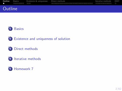
Outline
1 Basics
2 Existence and uniqueness of solution
3 Direct methods
4 Iterative methods
5 Homework 7
3/62
Outline Basics Existence & uniqueness Direct methods Iterative methods HW7
Outline
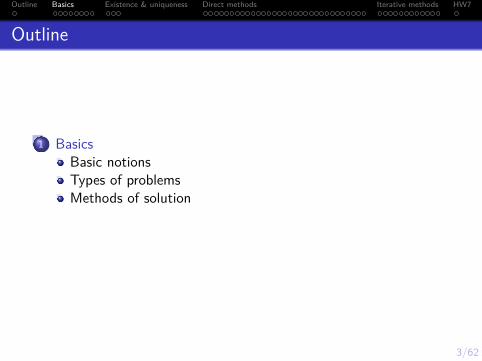
1 BasicsBasic notionsTypes of problemsMethods of solution
4/62
Outline Basics Existence & uniqueness Direct methods Iterative methods HW7
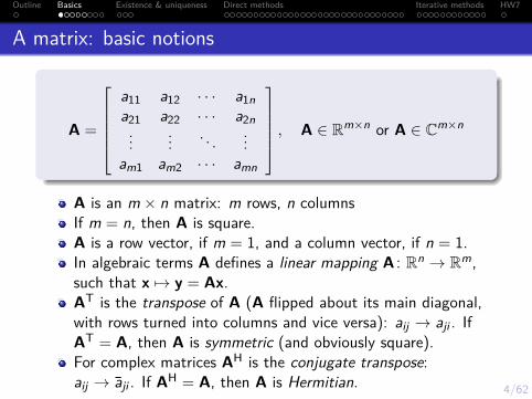
A matrix: basic notions
A =
a11 a12 · · · a1na21 a22 · · · a2n...
... . . . ...am1 am2 · · · amn
, A ∈ Rm×n or A ∈ Cm×n
A is an m × n matrix: m rows, n columnsIf m = n, then A is square.A is a row vector, if m = 1, and a column vector, if n = 1.In algebraic terms A defines a linear mapping A : Rn → Rm,such that x 7→ y = Ax.AT is the transpose of A (A flipped about its main diagonal,with rows turned into columns and vice versa): aij → aji . IfAT = A, then A is symmetric (and obviously square).For complex matrices AH is the conjugate transpose:aij → aji . If AH = A, then A is Hermitian.
5/62
Outline Basics Existence & uniqueness Direct methods Iterative methods HW7
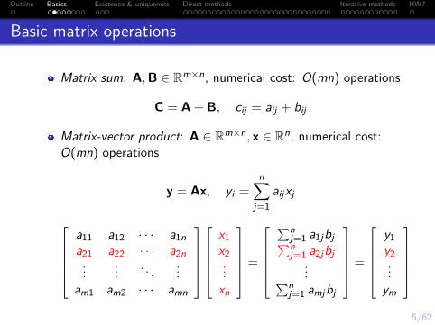
Basic matrix operations
Matrix sum: A,B ∈ Rm×n, numerical cost: O(mn) operations
C = A + B, cij = aij + bij
Matrix-vector product: A ∈ Rm×n, x ∈ Rn, numerical cost:O(mn) operations
y = Ax, yi =n∑
j=1aijxj
a11 a12 · · · a1na21 a22 · · · a2n...
... . . . ...am1 am2 · · · amn
x1x2...xn
=
∑n
j=1 a1jbj∑nj=1 a2jbj
...∑nj=1 amjbj
=
y1y2...
ym

6/62
Outline Basics Existence & uniqueness Direct methods Iterative methods HW7
Basic matrix operations
Matrix-matrix product: A ∈ Rm×n,B ∈ Rn×p, numerical cost:O(mnp) operations
C = AB, cij =n∑
k=1aikbkj
a11 a12 · · · a1na21 a22 · · · a2n...
... . . . ...am1 am2 · · · amn
b11 b12 · · · b1pb21 b22 · · · b2p...
... . . . ...bn1 bn2 · · · bnp
=
c11 c12 · · · c1nc21 c22 · · · a2n...
... . . . ...cm1 cm2 · · · cmp

7/62
Outline Basics Existence & uniqueness Direct methods Iterative methods HW7
Basic matrix operations
Matrix sumcommutative: A + B = B + Aassociative: A + (B + C) = (A + B) + C
Matrix productin general, not commutative:
if either A or B is non-square, both multiplications may not bepossible (incompatible dimensions)even if both matrices are square of the same dimensions,usually AB 6= BA
distributive: A(B + C) = AB + ACassociative: A(BC) = (AB)C(but the numerical cost can be very different)

8/62
Outline Basics Existence & uniqueness Direct methods Iterative methods HW7
Basic matrix operationsMatrix product is associative, but the numerical cost can be muchdifferent. Consider a matrix-matrix-vector product2:
A,B ∈ RN×N (matrices), C ∈ RN (a vector)A(BC) = (AB)C
Numerical cost of A(BC)
cost BC = O(N2)cost A(BC) = O(N2) + O(N2) = O(N2)
Numerical cost of (AB)C
cost AB = O(N3)cost (AB)C = O(N3) + O(N2) = O(N3)
2In C/C++, operator ∗ is left-associative, that is A ∗ B ∗ C = (A ∗ B) ∗ C.
9/62
Outline Basics Existence & uniqueness Direct methods Iterative methods HW7
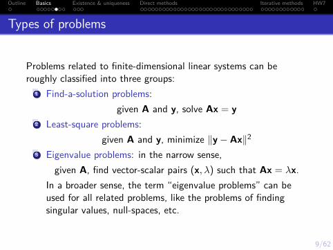
Types of problems
Problems related to finite-dimensional linear systems can beroughly classified into three groups:
1 Find-a-solution problems:given A and y, solve Ax = y
2 Least-square problems:given A and y, minimize ‖y− Ax‖2
3 Eigenvalue problems: in the narrow sense,given A, find vector-scalar pairs (x, λ) such that Ax = λx.
In a broader sense, the term “eigenvalue problems” can beused for all related problems, like the problems of findingsingular values, null-spaces, etc.
10/62
Outline Basics Existence & uniqueness Direct methods Iterative methods HW7
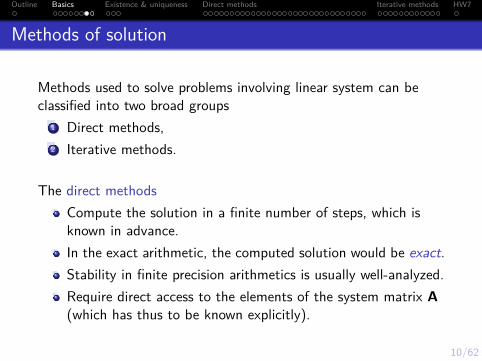
Methods of solution
Methods used to solve problems involving linear system can beclassified into two broad groups
1 Direct methods,2 Iterative methods.
The direct methodsCompute the solution in a finite number of steps, which isknown in advance.In the exact arithmetic, the computed solution would be exact.Stability in finite precision arithmetics is usually well-analyzed.Require direct access to the elements of the system matrix A(which has thus to be known explicitly).
11/62
Outline Basics Existence & uniqueness Direct methods Iterative methods HW7
Methods of solution
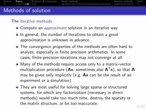
The iterative methodsCompute an approximate solution in an iterative way.In general, the number of iterations to obtain a goodapproximation is unknown in advance.The convergence properties of the methods are often hard toanalyze, especially in finite precision arithmetics. In somecases, finite-precision iterations may not converge at all.Many of the methods require access only to a matrix–vectormultiplication procedure (Ax, sometimes also ATx), so that Amay be given only implicitly (e.g. Ax can be the result of anexperiment or a simulation).They are most useful for solving large sparse or structuredsystems, for which any factorization (necessary in directmethods) would take too much time, destroy the sparsity orthe matrix structure, or be too inaccurate.

12/62
Outline Basics Existence & uniqueness Direct methods Iterative methods HW7
Outline
2 Existence and uniqueness of solution
13/62
Outline Basics Existence & uniqueness Direct methods Iterative methods HW7
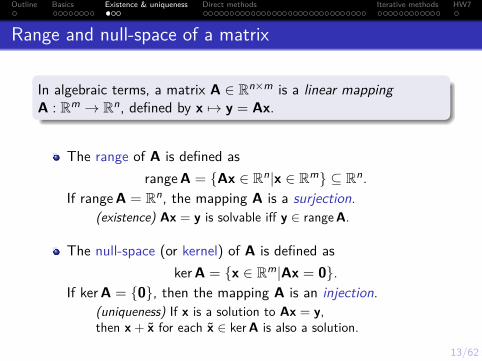
Range and null-space of a matrix
In algebraic terms, a matrix A ∈ Rn×m is a linear mappingA : Rm → Rn, defined by x 7→ y = Ax.
The range of A is defined asrange A = {Ax ∈ Rn|x ∈ Rm} ⊆ Rn.
If range A = Rn, the mapping A is a surjection.(existence) Ax = y is solvable iff y ∈ range A.
The null-space (or kernel) of A is defined asker A = {x ∈ Rm|Ax = 0}.
If ker A = {0}, then the mapping A is an injection.(uniqueness) If x is a solution to Ax = y,then x + x for each x ∈ ker A is also a solution.
14/62
Outline Basics Existence & uniqueness Direct methods Iterative methods HW7
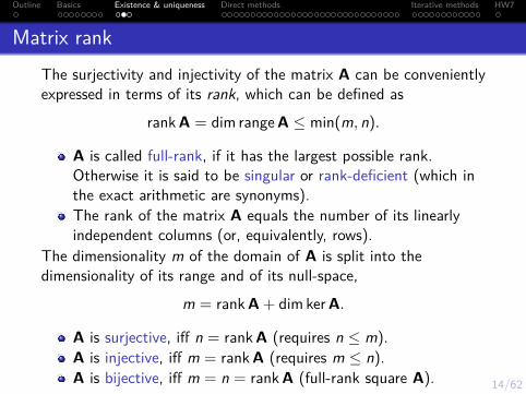
Matrix rankThe surjectivity and injectivity of the matrix A can be convenientlyexpressed in terms of its rank, which can be defined as
rank A = dim range A ≤ min(m, n).
A is called full-rank, if it has the largest possible rank.Otherwise it is said to be singular or rank-deficient (which inthe exact arithmetic are synonyms).The rank of the matrix A equals the number of its linearlyindependent columns (or, equivalently, rows).
The dimensionality m of the domain of A is split into thedimensionality of its range and of its null-space,
m = rank A + dim ker A.
A is surjective, iff n = rank A (requires n ≤ m).A is injective, iff m = rank A (requires m ≤ n).A is bijective, iff m = n = rank A (full-rank square A).
15/62
Outline Basics Existence & uniqueness Direct methods Iterative methods HW7
Existence and uniqueness of solution
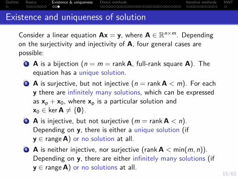
Consider a linear equation Ax = y, where A ∈ Rn×m. Dependingon the surjectivity and injectivity of A, four general cases arepossible:
1 A is a bijection (n = m = rank A, full-rank square A). Theequation has a unique solution.
2 A is surjective, but not injective (n = rank A < m). For eachy there are infinitely many solutions, which can be expressedas xp + x0, where xp is a particular solution andx0 ∈ ker A 6= {0}.
3 A is injective, but not surjective (m = rank A < n).Depending on y, there is either a unique solution (ify ∈ range A) or no solution at all.
4 A is neither injective, nor surjective (rank A < min(m, n)).Depending on y, there are either infinitely many solutions (ify ∈ range A) or no solutions at all.
16/62
Outline Basics Existence & uniqueness Direct methods Iterative methods HW7
Outline
3 Direct methodsSpecial matricesFactorizations and decompositionsGaussian elimination
17/62
Outline Basics Existence & uniqueness Direct methods Iterative methods HW7
Direct methods
Direct methodsCompute the solution in a finite and known in advance time(number of steps).In the exact arithmetic, the computed solution would be exact.Stability in finite precision arithmetics are usuallywell-analyzed.Require direct access to the elements of the system matrix A(which has thus to be explicitly given).
18/62
Outline Basics Existence & uniqueness Direct methods Iterative methods HW7
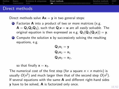
Direct methods
Direct methods solve Ax = y in two general steps:1 Factorize A into a product of two or more matrices (e.g.
A = Q1Q2Q3), such that Qiv = u are all easily solvable. Theoriginal equation is then expressed as e.g. Q1(Q2(Q3x)) = y.
2 Compute the solution x by successively solving the resultingequations, e.g.
Q1x1 = yQ2x2 = x1
Q3x3 = x2,
so that finally x = x3.The numerical cost of the first step (for a square n × n matrix) isusually O(n3) and much larger then that of the second step O(n2).If several equations with the same A and different right-hand sidesy have to be solved, A is factorized only once.

19/62
Outline Basics Existence & uniqueness Direct methods Iterative methods HW7
Special matrices
In the first step, a direct method of solving Ax = y factorizes Ainto a product of two or more special matrices Q1,Q2, . . . ,QN .
The matrices are called special, since Qiv = u have all to be easilysolvable. They are usually:
diagonal,unitary or orthonormal,permutation matrices,lower or upper triangular.

20/62
Outline Basics Existence & uniqueness Direct methods Iterative methods HW7
Square diagonal matrices
D = diag(d1, d2, . . . , dn) =
d1 0
d2. . .
0 dn
Elements of a diagonal matrix are all zero except the diagonal.If di 6= 0 for all i , then D is full-rank and bijective. Thesystem Dx = y is then uniquely solvable for all y.If di = 0 for some i , then D is singular and neither surjectivenor bijective. Depending on y, the system Dx = y has eitherinfinitely many solutions or no solutions at all.
21/62
Outline Basics Existence & uniqueness Direct methods Iterative methods HW7
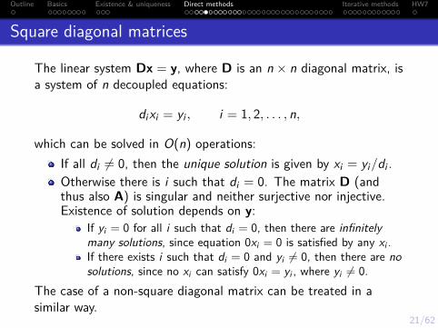
Square diagonal matrices
The linear system Dx = y, where D is an n × n diagonal matrix, isa system of n decoupled equations:
dixi = yi , i = 1, 2, . . . , n,
which can be solved in O(n) operations:If all di 6= 0, then the unique solution is given by xi = yi/di .Otherwise there is i such that di = 0. The matrix D (andthus also A) is singular and neither surjective nor injective.Existence of solution depends on y:
If yi = 0 for all i such that di = 0, then there are infinitelymany solutions, since equation 0xi = 0 is satisfied by any xi .If there exists i such that di = 0 and yi 6= 0, then there are nosolutions, since no xi can satisfy 0xi = yi , where yi 6= 0.
The case of a non-square diagonal matrix can be treated in asimilar way.

22/62
Outline Basics Existence & uniqueness Direct methods Iterative methods HW7
Diagonal matrices — examples
Square diagonal matrix1 0 0 00 2 0 00 0 0 00 0 0 4
x1x2x3x4
=
11y1
If y == 0, then the equation has infinitely many solutions:
x1x2x3x4
=
1
1/20
1/4
+
00c0
, c ∈ R,
where [1 1/2 0 1/3]T is a particular solution and [0 0 c 0]T belongsto the null space of the system matrix. Otherwise (if y 6= 0), theequation nas no solutions.
22/62
Outline Basics Existence & uniqueness Direct methods Iterative methods HW7
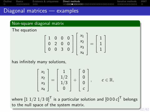
Diagonal matrices — examples
Non-square diagonal matrixThe equation 1 0 0 0
0 2 0 00 0 3 0
x1x2x3x4
=
111
has infinitely many solutions,
x1x2x3x4
=
1
1/21/30
+
000c
, c ∈ R,
where [1 1/2 1/3 0]T is a particular solution and [0 0 0 c]T belongsto the null space of the system matrix.
22/62
Outline Basics Existence & uniqueness Direct methods Iterative methods HW7
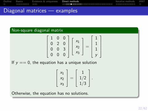
Diagonal matrices — examples
Non-square diagonal matrix1 0 00 2 00 0 30 0 0
x1
x2x3
=
111y
If y == 0, the equation has a unique solution x1
x2x3
=
11/21/3
.Otherwise, the equation has no solutions.
23/62
Outline Basics Existence & uniqueness Direct methods Iterative methods HW7
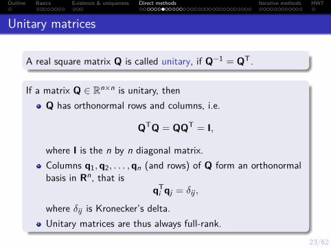
Unitary matrices
A real square matrix Q is called unitary, if Q−1 = QT.
If a matrix Q ∈ Rn×n is unitary, thenQ has orthonormal rows and columns, i.e.
QTQ = QQT = I,
where I is the n by n diagonal matrix.Columns q1,q2, . . . ,qn (and rows) of Q form an orthonormalbasis in Rn, that is
qTi qj = δij ,
where δij is Kronecker’s delta.Unitary matrices are thus always full-rank.

24/62
Outline Basics Existence & uniqueness Direct methods Iterative methods HW7
Unitary and orthonormal matrices
Since unitary matrices are always full-rank and easily invertible(Q−1 = QT), a linear system Qx = y with a unitary matrixQ ∈ Rn×n has a unique solution for all y and can be solved inO(n2) operations,
x = Q−1y = QTy.
A unitary matrix with a part of rows (or columns) removed iscalled an orthonormal matrix. The removed (or, more often, notcomputed at all) vectors usually form a basis of the null-space ofthe considered system matrix. They can be thus disregarded, ifonly a particular solution is sought for instead of the full solutionspace. The particular solution obtained this way is usually theminimum-norm solution.

25/62
Outline Basics Existence & uniqueness Direct methods Iterative methods HW7
Permutation matrices
A square n× n matrix Π is said to be a permutation matrix, if it isobtained from an n × n identity matrix by permuting its rows.
Every row and every column of a permutation matrix hasexactly single 1 and everywhere else 0s.There are n! different permutations of an n-element sequence.So, there are exactly n! permutation matrices of thedimensions n × n.A permutation matrix Π satisfies ΠTΠ = I, therefore it is aspecial case of a unitary matrix.When applied to an n × n matrix A:
ΠA is the matrix A with permuted rows.AΠ is the matrix A with permuted columns.

26/62
Outline Basics Existence & uniqueness Direct methods Iterative methods HW7
Lower and upper triangular matrices
A square matrix L is called a lower triangular matrix, if all itselements above the main diagonal are zero: lij = 0 for i < j .
A square matrix U is called an upper triangular matrix, if all itselements below the main diagonal are zero: uij = 0 for i > j .
L =
l11 0l21 l22...
... . . .ln1 ln2 · · · lnn
U =
u11 u12 · · · u1n
u22 · · · u2n. . . ...
0 unn

27/62
Outline Basics Existence & uniqueness Direct methods Iterative methods HW7
Lower triangular systems — forward-substitution
An n × n lower triangular system Lx = y,l11 0l21 l22...
... . . .ln1 ln2 · · · lnn
x1x2...xn
=
y1y2...yn
,
can be solved with O(n2) operations by forward-substitution.
Forward substitution
x1 = y1l11, xi =
yi −∑i−1
j=1 lijxj
lii.
28/62
Outline Basics Existence & uniqueness Direct methods Iterative methods HW7
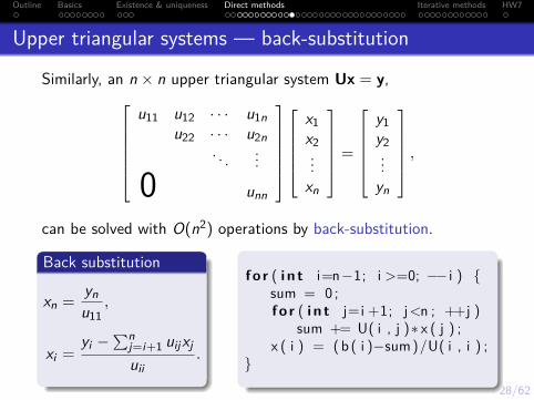
Upper triangular systems — back-substitution
Similarly, an n × n upper triangular system Ux = y,u11 u12 · · · u1n
u22 · · · u2n. . . ...
0 unn
x1x2...xn
=
y1y2...yn
,
can be solved with O(n2) operations by back-substitution.
Back substitution
xn = ynu11
,
xi =yi −
∑nj=i+1 uijxj
uii.
f o r ( i n t i=n−1; i >=0; −− i ) {sum = 0 ;f o r ( i n t j=i +1; j<n ; ++j )
sum += U( i , j )∗ x ( j ) ;x ( i ) = (b ( i )−sum)/U( i , i ) ;
}
29/62
Outline Basics Existence & uniqueness Direct methods Iterative methods HW7
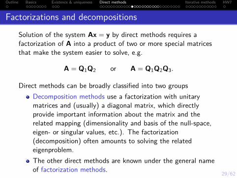
Factorizations and decompositions
Solution of the system Ax = y by direct methods requires afactorization of A into a product of two or more special matricesthat make the system easier to solve, e.g.
A = Q1Q2 or A = Q1Q2Q3.
Direct methods can be broadly classified into two groupsDecomposition methods use a factorization with unitarymatrices and (usually) a diagonal matrix, which directlyprovide important information about the matrix and therelated mapping (dimensionality and basis of the null-space,eigen- or singular values, etc.). The factorization(decomposition) often amounts to solving the relatedeigenproblem.The other direct methods are known under the general nameof factorization methods.
30/62
Outline Basics Existence & uniqueness Direct methods Iterative methods HW7
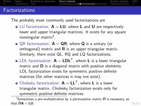
FactorizationsThe probably most commonly used factorizations are
LU factorization: A = LU, where L and U are respectivelylower and upper triangular matrices. It exists for any squarenonsingular matrix3.QR factorization: A = QR, where Q is a unitary (ororthogonal) matrix and R is an upper triangular matrix.Similarly, there exist QL, RQ and LQ factorizations.LDL factorization: A = LDLT, where L is a lower triangularmatrix and D is a diagonal matrix with positive elements.LDL factorization exists for symmetric positive definitematrices (for other matrices it may not exist).Cholesky factorization: A = LLT, where L is a lowertriangular matrix. Cholesky factorization exists only forsymmetric positive definite matrices.
3Sometimes a pre-multiplication by a permutation matrix Π is necessary, sothat ΠA = LU.

31/62
Outline Basics Existence & uniqueness Direct methods Iterative methods HW7
Decompositions — eigen decompositionEigenvalues and eigenvectors
A fundamental notion in linear algebra is that of an eigenvalue andthe corresponding eigenvectors of a square matrix.
Let A be a square n × n matrix. A number λ is called aneigenvalue of A and a vector v is called a correspondingeigenvector if and only if Av = λv.
As the above condition yields (A− λI) v = 0, the eigenvalues of Aare the roots of its characteristic polynomial,
fA(λ) = det (A− λI) ,
which always has n complex roots. Thus, every square n × nmatrix has always n complex eigenvalues (some or all of which canbe real). Every eigenvalue has a multiplicity, which is defined asthe multiplicity of the corresponding root of fA(λ).
32/62
Outline Basics Existence & uniqueness Direct methods Iterative methods HW7
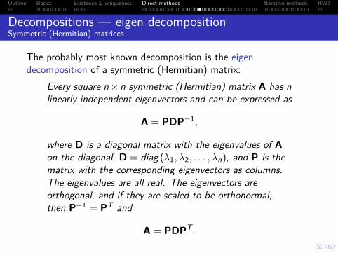
Decompositions — eigen decompositionSymmetric (Hermitian) matrices
The probably most known decomposition is the eigendecomposition of a symmetric (Hermitian) matrix:
Every square n× n symmetric (Hermitian) matrix A has nlinearly independent eigenvectors and can be expressed as
A = PDP−1,
where D is a diagonal matrix with the eigenvalues of Aon the diagonal, D = diag (λ1, λ2, . . . , λn), and P is thematrix with the corresponding eigenvectors as columns.The eigenvalues are all real. The eigenvectors areorthogonal, and if they are scaled to be orthonormal,then P−1 = PT and
A = PDPT.

33/62
Outline Basics Existence & uniqueness Direct methods Iterative methods HW7
Decompositions — eigen decomposition
If A is non-symmetric (non-Hermitian), the existence of the eigendecomposition depends on the number of the eigenvectors:
If a square n × n matrix A has n linearly independenteigenvectors, than it can be expressed as
A = PDP−1,
where P collects all the eigenvectors as columns, and Dis a diagonal matrix with the corresponding eigenvalueson the diagonal, D = diag (λ1, λ2, . . . , λn).
If A has an eigen decomposition, it is called diagonalizable4. Anon-symmetric (non-Hermitian) matrix may have complexeigenvalues.
4It is diagonal in the coordinates defined by the columns of P.
34/62
Outline Basics Existence & uniqueness Direct methods Iterative methods HW7
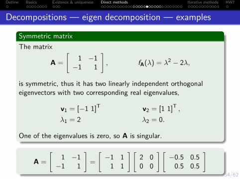
Decompositions — eigen decomposition — examples
Symmetric matrixThe matrix
A =[
1 −1−1 1
], fA(λ) = λ2 − 2λ,
is symmetric, thus it has two linearly independent orthogonaleigenvectors with two corresponding real eigenvalues,
v1 = [−1 1]T v2 = [1 1]T ,λ1 = 2 λ2 = 0.
One of the eigenvalues is zero, so A is singular.
A =[
1 −1−1 1
]=[−1 1
1 1
] [2 00 0
] [−0.5 0.5
0.5 0.5
]

34/62
Outline Basics Existence & uniqueness Direct methods Iterative methods HW7
Decompositions — eigen decomposition — examples
Non-symmetric diagonalizable matrixThe non-symmetric matrix
A =[
1 1−1 1
], fA(λ) = λ2 − 2λ+ 2,
is diagonalizable, since it has two linearly independent eigenvectors,
v1 = [−i 1]T v2 = [i 1]T .
The two corresponding eigenvalues are complex:
λ1 = 1 + i λ2 = 1− i.
A =[
1 1−1 1
]=[−i i1 1
] [1 + i 0
0 1− i
] [0.5i 0.5−0.5i 0.5
]
34/62
Outline Basics Existence & uniqueness Direct methods Iterative methods HW7
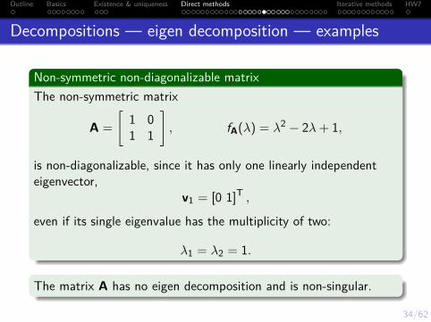
Decompositions — eigen decomposition — examples
Non-symmetric non-diagonalizable matrixThe non-symmetric matrix
A =[
1 01 1
], fA(λ) = λ2 − 2λ+ 1,
is non-diagonalizable, since it has only one linearly independenteigenvector,
v1 = [0 1]T ,
even if its single eigenvalue has the multiplicity of two:
λ1 = λ2 = 1.
The matrix A has no eigen decomposition and is non-singular.
35/62
Outline Basics Existence & uniqueness Direct methods Iterative methods HW7
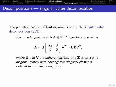
Decompositions — singular value decomposition
The probably most important decomposition is the singular valuedecomposition (SVD):
Every rectangular matrix A ∈ Rn×m can be expressed as
A = U[
Σ0 00 0
]VT = UΣVT,
where U and V are unitary matrices, and Σ is an n ×mdiagonal matrix with nonnegative diagonal elementsordered in a nonincreasing way.

36/62
Outline Basics Existence & uniqueness Direct methods Iterative methods HW7
Decompositions — singular value decomposition
Every rectangular matrix A ∈ Rn×m can be expressed as
A = U[
Σ0 00 0
]VT = UΣVT,
where U and V are unitary, and Σ is a diagonal matrix.
full-rank A ∈ Rn×m (rank A = n < m)
A = UΣVT =

37/62
Outline Basics Existence & uniqueness Direct methods Iterative methods HW7
Decompositions — singular value decompositionEvery rectangular matrix A ∈ Rn×m can be expressed as
A = U[
Σ0 00 0
]VT = UΣVT,
where U and V are unitary, and Σ is a diagonal matrix.Diagonal elements σi of Σ are called the singular values of A.The number r of positive singular values equals to rank A.The matrix Σ0 is thus rank A× rank A.The SVD is unique up to the ordering of the singular vectors(columns of U and V) corresponding to equal singular values.The columns of V, which correspond to the vanishing singularvalues, form a basis for the null-space of A.ATA = VΣTUTUΣVT = VΣTΣVT is the eigendecomposition of ATA. Therefore, σ2
i (A) = λi (ATA).The singular values provide full information aboutconditioning of A (see Lecture B-4).
38/62
Outline Basics Existence & uniqueness Direct methods Iterative methods HW7
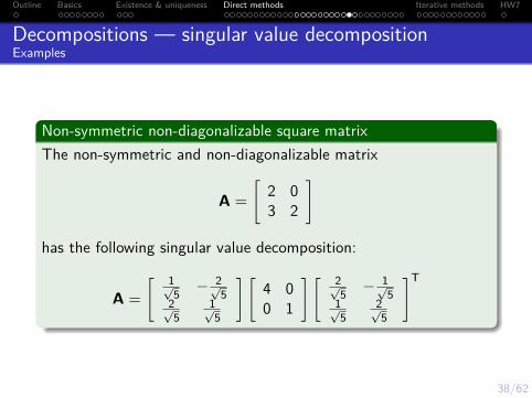
Decompositions — singular value decompositionExamples
Non-symmetric non-diagonalizable square matrixThe non-symmetric and non-diagonalizable matrix
A =[
2 03 2
]
has the following singular value decomposition:
A =[ 1√
5 − 2√5
2√5
1√5
] [4 00 1
] [ 2√5 − 1√
51√5
2√5
]T
38/62
Outline Basics Existence & uniqueness Direct methods Iterative methods HW7
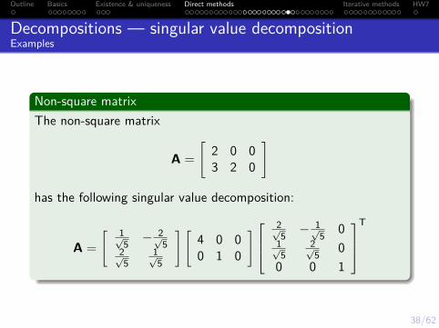
Decompositions — singular value decompositionExamples
Non-square matrixThe non-square matrix
A =[
2 0 03 2 0
]
has the following singular value decomposition:
A =[ 1√
5 − 2√5
2√5
1√5
] [4 0 00 1 0
]2√5 − 1√
5 01√5
2√5 0
0 0 1
T
39/62
Outline Basics Existence & uniqueness Direct methods Iterative methods HW7
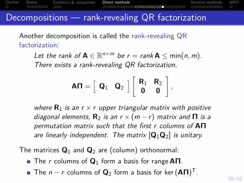
Decompositions — rank-revealing QR factorization
Another decomposition is called the rank-revealing QRfactorization:
Let the rank of A ∈ Rn×m be r = rank A ≤ min(n,m).There exists a rank-revealing QR factorization,
AΠ =[
Q1 Q2] [ R1 R2
0 0
],
where R1 is an r × r upper triangular matrix with positivediagonal elements, R2 is an r × (m− r) matrix and Π is apermutation matrix such that the first r columns of AΠare linearly independent. The matrix [Q1Q2] is unitary.
The matrices Q1 and Q2 are (column) orthonormal:The r columns of Q1 form a basis for range AΠ.The n − r columns of Q2 form a basis for ker (AΠ)T.

40/62
Outline Basics Existence & uniqueness Direct methods Iterative methods HW7
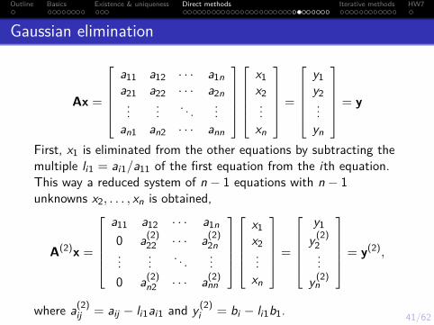
Gaussian elimination
Gaussian elimination is a method ofsolving a full-rank Ax = y byperforming the LU factorization of A.
Gaussian elimination uses two elementary operations1 adding a multiple of the ith row to the jth row and2 interchanging two rows/equations (or columns/unknowns),
called pivotingto eliminate the unknowns xi in order to obtain an equivalentupper triangular system Ux = y, which can be solved byback-substitution.
41/62
Outline Basics Existence & uniqueness Direct methods Iterative methods HW7
Gaussian elimination
Ax =
a11 a12 · · · a1na21 a22 · · · a2n...
... . . . ...an1 an2 · · · ann
x1x2...xn
=
y1y2...yn
= y
First, x1 is eliminated from the other equations by subtracting themultiple li1 = ai1/a11 of the first equation from the ith equation.This way a reduced system of n − 1 equations with n − 1unknowns x2, . . . , xn is obtained,
A(2)x =
a11 a12 · · · a1n
0 a(2)22 · · · a(2)
2n...
... . . . ...0 a(2)
n2 · · · a(2)nn
x1x2...xn
=
y1
y (2)2...
y (2)n
= y(2),
where a(2)ij = aij − li1ai1 and y (2)
i = bi − li1b1.

42/62
Outline Basics Existence & uniqueness Direct methods Iterative methods HW7
Gaussian elimination
The procedure is repeated n − 1 times: xk , k = 2, . . . , n − 1 iseliminated from the rest i = k + 1, . . . , n equations using themultiplier lik = a(k)
ik /a(k)kk . This yields an upper triangular system,
which can be solved by back-substitution:
A(n)x =
a11 a12 · · · a1n
a(2)22 · · · a(2)
2n. . . ...
0 a(n)nn
x1x2...xn
=
y1
y (2)2...
y (n)n
= y(n),
where a(k+1)ij = a(k)
ij − lika(k)ik and y (k+1)
i = b(k)i − likb(k)
k .
43/62
Outline Basics Existence & uniqueness Direct methods Iterative methods HW7
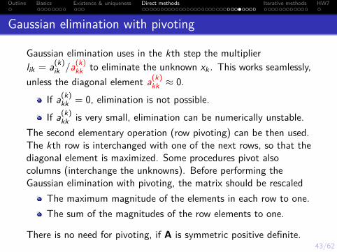
Gaussian elimination with pivoting
Gaussian elimination uses in the kth step the multiplierlik = a(k)
ik /a(k)kk to eliminate the unknown xk . This works seamlessly,
unless the diagonal element a(k)kk ≈ 0.
If a(k)kk = 0, elimination is not possible.
If a(k)kk is very small, elimination can be numerically unstable.
The second elementary operation (row pivoting) can be then used.The kth row is interchanged with one of the next rows, so that thediagonal element is maximized. Some procedures pivot alsocolumns (interchange the unknowns). Before performing theGaussian elimination with pivoting, the matrix should be rescaled
The maximum magnitude of the elements in each row to one.The sum of the magnitudes of the row elements to one.
There is no need for pivoting, if A is symmetric positive definite.
44/62
Outline Basics Existence & uniqueness Direct methods Iterative methods HW7
Gaussian elimination with pivoting — example
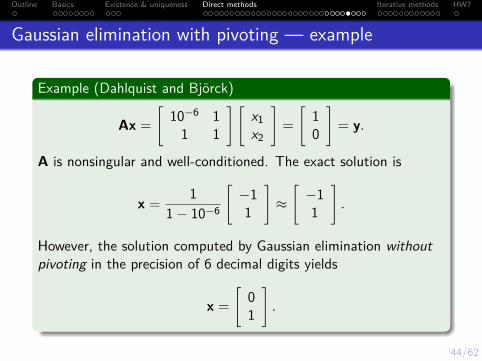
Example (Dahlquist and Björck)
Ax =[
10−6 11 1
] [x1x2
]=[
10
]= y.
A is nonsingular and well-conditioned. The exact solution is
x = 11− 10−6
[−11
]≈[−11
].
However, the solution computed by Gaussian elimination withoutpivoting in the precision of 6 decimal digits yields
x =[
01
].

45/62
Outline Basics Existence & uniqueness Direct methods Iterative methods HW7
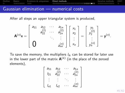
Gaussian elimination — numerical costs
After all steps an upper triangular system is produced,
A(n)x =
a11 a12 · · · a1n
a(2)22 · · · a(2)
2n. . . ...
0 a(n)nn
x1x2...xn
=
y1
y (2)2...
y (n)n
= y(n).
The number of operations in Gaussian elimination is ∼ n3/3. Thisis substantially more than ∼ n2/2 necessary to solve the resultingupper triangular system.If the multipliers lik are stored (together with the informationabout row interchange and scaling, if necessary), then y(n) fordifferent right-hand side vectors y can be computed at later timesat the cost of ∼ n2/2 only. Hence the total cost of eachsubsequent computation would be ∼ n2 only.
45/62
Outline Basics Existence & uniqueness Direct methods Iterative methods HW7
Gaussian elimination — numerical costs
After all steps an upper triangular system is produced,
A(n)x =
a11 a12 · · · a1n
a(2)22 · · · a(2)
2n. . . ...
0 a(n)nn
x1x2...xn
=
y1
y (2)2...
y (n)n
= y(n).
To save the memory, the multipliers lik can be stored for later usein the lower part of the matrix A(k) (in the place of the zeroedelements),
a11 a12 · · · a1n
l21 a(2)22 · · · a(2)
2n...
... . . . ...ln1 ln2 · · · a(n)
nn

46/62
Outline Basics Existence & uniqueness Direct methods Iterative methods HW7
Gaussian elimination — LU factorizationGaussian elimination is an algorithm for LU factorization of thesystem matrix, A = LU, where:
L = [lik ], where lkk = 1 and lik = 0 for i < k.U = [ukj ], where ukj = a(k)
kj for j ≥ k and ukj = 0 otherwise.
A(n) →
a11 a12 · · · a1n
l21 a(2)22 · · · a(2)
2n...
... . . . ...ln1 ln2 · · · a(n)
nn
→
1 0l21 1...
... . . .ln1 ln2 · · · 1
a11 a12 · · · a1n
a(2)22 · · · a(2)
2n. . . ...
0 a(n)nn
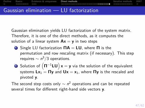
47/62
Outline Basics Existence & uniqueness Direct methods Iterative methods HW7
Gaussian elimination — LU factorization
Gaussian elimination yields LU factorization of the system matrix.Therefore, it is one of the direct methods, as it computes thesolution of a linear system Ax = y in two steps
1 Single LU factorization ΠA = LU, where Π is thepermutation and row rescaling matrix (if necessary). This steprequires ∼ n3/3 operations.
2 Solution of(Π−1LU
)x = y via the solution of the equivalent
systems Lx1 = Πy and Ux = x1, where Πy is the rescaled andpivoted y.
The second step costs only ∼ n2 operations and can be repeatedseveral times for different right-hand side vectors y.
48/62
Outline Basics Existence & uniqueness Direct methods Iterative methods HW7
Outline
4 Iterative methodsStationary methodsKrylov subspace methods
49/62
Outline Basics Existence & uniqueness Direct methods Iterative methods HW7
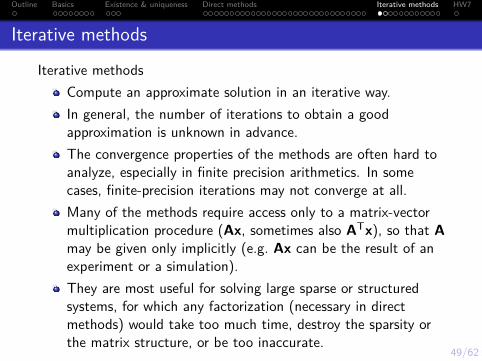
Iterative methods
Iterative methodsCompute an approximate solution in an iterative way.In general, the number of iterations to obtain a goodapproximation is unknown in advance.The convergence properties of the methods are often hard toanalyze, especially in finite precision arithmetics. In somecases, finite-precision iterations may not converge at all.Many of the methods require access only to a matrix-vectormultiplication procedure (Ax, sometimes also ATx), so that Amay be given only implicitly (e.g. Ax can be the result of anexperiment or a simulation).They are most useful for solving large sparse or structuredsystems, for which any factorization (necessary in directmethods) would take too much time, destroy the sparsity orthe matrix structure, or be too inaccurate.

50/62
Outline Basics Existence & uniqueness Direct methods Iterative methods HW7
Iterative methods
There are two important groups of iterative methodsStationary methods: Jacobi, Gauss-Seidel, successiveover-relaxation (SOR), etc.Krylov subspace methods, out of which the conjugate gradientmethod seems to be the most important.
51/62
Outline Basics Existence & uniqueness Direct methods Iterative methods HW7
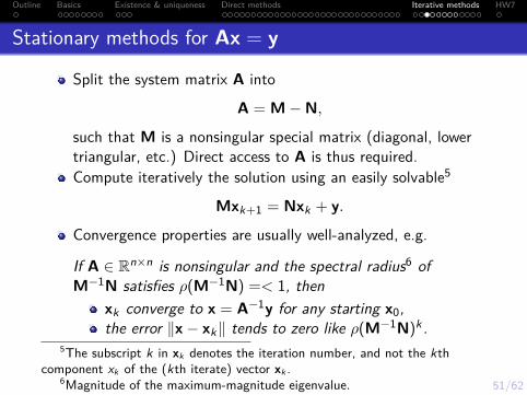
Stationary methods for Ax = y
Split the system matrix A into
A = M−N,
such that M is a nonsingular special matrix (diagonal, lowertriangular, etc.) Direct access to A is thus required.Compute iteratively the solution using an easily solvable5
Mxk+1 = Nxk + y.
Convergence properties are usually well-analyzed, e.g.
If A ∈ Rn×n is nonsingular and the spectral radius6 ofM−1N satisfies ρ(M−1N) =< 1, then
xk converge to x = A−1y for any starting x0,the error ‖x− xk‖ tends to zero like ρ(M−1N)k .
5The subscript k in xk denotes the iteration number, and not the kthcomponent xk of the (kth iterate) vector xk .
6Magnitude of the maximum-magnitude eigenvalue.

52/62
Outline Basics Existence & uniqueness Direct methods Iterative methods HW7
Stationary methods — Jacobi and Gauss-SeidelStationary methods for Ax = y are defined by
Mxk+1 = Nxk + y, where A = M−N.
Split the system matrix A into its strictly lower triangular L,diagonal D and strictly upper triangular U parts,
A = L + D + U.
The Jacobi method is defined by
M = D,N = −L−U.
The Gauss-Seidel method is defined by
M = D + L,N = −U.
Both method are convergent if A is symmetric positive-definite.
53/62
Outline Basics Existence & uniqueness Direct methods Iterative methods HW7
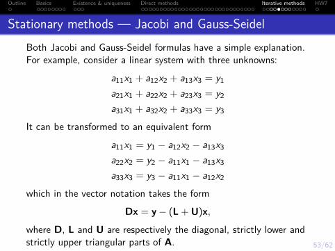
Stationary methods — Jacobi and Gauss-SeidelBoth Jacobi and Gauss-Seidel formulas have a simple explanation.For example, consider a linear system with three unknowns:
a11x1 + a12x2 + a13x3 = y1
a21x1 + a22x2 + a23x3 = y2
a31x1 + a32x2 + a33x3 = y3
It can be transformed to an equivalent form
a11x1 = y1 − a12x2 − a13x3
a22x2 = y2 − a11x1 − a13x3
a33x3 = y3 − a11x1 − a12x2
which in the vector notation takes the form
Dx = y− (L + U)x,
where D, L and U are respectively the diagonal, strictly lower andstrictly upper triangular parts of A.

54/62
Outline Basics Existence & uniqueness Direct methods Iterative methods HW7
Stationary methods — Jacobi and Gauss-SeidelTherefore, every linear system Ax = y can be transformed to theequivalent form
Dx = y− (L + U)x.
The Jacobi method takes this formula directly and obtains
Dxk+1 = y− (L + U)xk ,
where all components of xk+1 are computed using theprevious-step iterate xk . However, when the ith component of thevector xk+1 is being computed, then all the components precedingit (no. 1, 2, . . . , i − 1) are already known and can be used insteadof these of the previous-step iterate xk . This yields theGauss-Seidel method,
Dxk+1 = y− Lxk+1 −Uxk , that is(D + U)xk+1 = y−Uxk .
55/62
Outline Basics Existence & uniqueness Direct methods Iterative methods HW7
Stationary methods — successive over-relaxation (SOR)
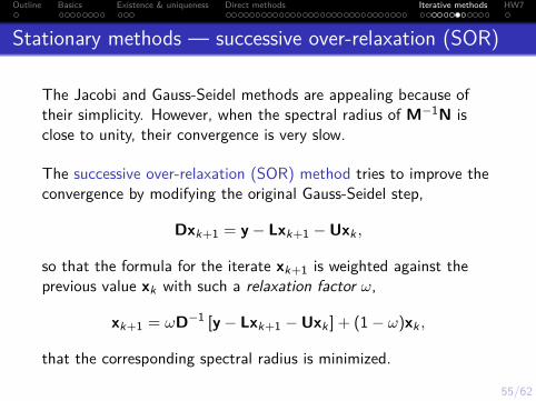
The Jacobi and Gauss-Seidel methods are appealing because oftheir simplicity. However, when the spectral radius of M−1N isclose to unity, their convergence is very slow.
The successive over-relaxation (SOR) method tries to improve theconvergence by modifying the original Gauss-Seidel step,
Dxk+1 = y− Lxk+1 −Uxk ,
so that the formula for the iterate xk+1 is weighted against theprevious value xk with such a relaxation factor ω,
xk+1 = ωD−1 [y− Lxk+1 −Uxk ] + (1− ω)xk ,
that the corresponding spectral radius is minimized.

56/62
Outline Basics Existence & uniqueness Direct methods Iterative methods HW7
Stationary methods — successive over-relaxation (SOR)
The SOR method can be compactly represented in the generalform of the stationary methods,
Mωxk+1 = Nωxk + ωy,
where
Mω = D + ωL,Nω = (1− ω)D− ωU.
The relaxation factor ω should minimize the spectral radius ofM−1
ω Nω. The choice of its optimum value is not easy. In generalSOR can be convergent only for ω ∈ (0, 2).If A is symmetric positive-definite, then SOR converges for allω ∈ (0, 2).
57/62
Outline Basics Existence & uniqueness Direct methods Iterative methods HW7
Krylov subspace methods
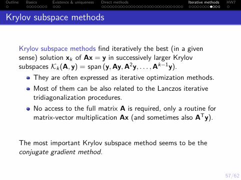
Krylov subspace methods find iteratively the best (in a givensense) solution xk of Ax = y in successively larger Krylovsubspaces Kk(A, y) = span (y,Ay,A2y, . . . ,Ak−1y).
They are often expressed as iterative optimization methods.Most of them can be also related to the Lanczos iterativetridiagonalization procedures.No access to the full matrix A is required, only a routine formatrix-vector multiplication Ax (and sometimes also ATy).
The most important Krylov subspace method seems to be theconjugate gradient method.
58/62
Outline Basics Existence & uniqueness Direct methods Iterative methods HW7
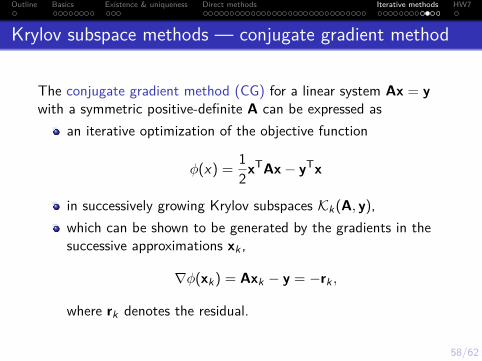
Krylov subspace methods — conjugate gradient method
The conjugate gradient method (CG) for a linear system Ax = ywith a symmetric positive-definite A can be expressed as
an iterative optimization of the objective function
φ(x) = 12xTAx− yTx
in successively growing Krylov subspaces Kk(A, y),which can be shown to be generated by the gradients in thesuccessive approximations xk ,
∇φ(xk) = Axk − y = −rk ,
where rk denotes the residual.
59/62
Outline Basics Existence & uniqueness Direct methods Iterative methods HW7
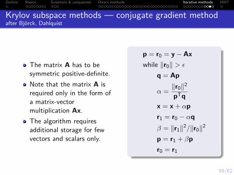
Krylov subspace methods — conjugate gradient methodafter Björck, Dahlquist
The matrix A has to besymmetric positive-definite.Note that the matrix A isrequired only in the form ofa matrix-vectormultiplication Ax.The algorithm requiresadditional storage for fewvectors and scalars only.
p = r0 = y− Axwhile ‖r0‖ > ε
q = Ap
α = ‖r0‖2
pTqx = x + αpr1 = r0 − αqβ = ‖r1‖2/‖r0‖2
p = r1 + βpr0 = r1

60/62
Outline Basics Existence & uniqueness Direct methods Iterative methods HW7
Krylov subspace methods — CGLS methodafter Björck, Dahlquist
If A is not symmetricpositive-definite, then the CGmethod can be applied to thenormal equations,
ATAx = ATy,
which amounts to minimizing
φ(x) = 12‖Ax− y‖2.
This is the conjugate gradientleast-squares (CGLS) method.A is required only in the form ofthe multiplications Ax and ATy.
r = y− Axp = s0 = ATrwhile ‖r‖ > ε
q = Apα = ‖s0‖2/‖q‖2
x = x + αpr = r − αqs1 = ATrβ = ‖s1‖2/‖s0‖2
p = s1 + βps0 = s1

61/62
Outline Basics Existence & uniqueness Direct methods Iterative methods HW7
Outline
5 Homework 7

62/62
Outline Basics Existence & uniqueness Direct methods Iterative methods HW7
Homework 7 (25 points)LU decomposition
Available soon at http://info.ippt.pan.pl/˜ljank.
E-mail the answer and the source codes to [email protected].