proj mani
TRANSCRIPT
Analysis Top kerf Width
Response 1 top KW ANOVA for Response Surface Reduced Cubic ModelAnalysis of variance table [Partial sum of squares - Type III]
Sum of Mean F p-valueSource Squares df Square Value Prob > FModel 0.22 12 0.018 3.32 0.1285 not
significantA-power 0.089 1 0.089 16.27 0.0157B-cutting speed 9.801E-003 1 9.801E-003 1.78 0.2527C-gas pressure 9.216E-003 1 9.216E-003 1.68 0.2650
AB 3.422E-004 1 3.422E-004 0.062 0.8152AC 0.015 1 0.015 2.80 0.1697BC 0.019 1 0.019 3.47 0.1362A2 0.019 1 0.019 3.53 0.1335B2 4.753E-004 1 4.753E-004 0.086 0.7833C2 0.041 1 0.041 7.53 0.0517
A2B 0.010 1 0.010 1.87 0.2429A2C 4.705E-003 1 4.705E-003 0.86 0.4072AB2 0.020 1 0.020 3.66 0.1284
Pure Error 0.022 4 5.495E-003Cor Total 0.24 16
The "Model F-value" of 3.32 implies the model is not significant relative to the noise. There is a12.85 % chance that a "Model F-value" this large could occur due to noise.
Values of "Prob > F" less than 0.0500 indicate model terms are significant. In this case A are significant model terms. Values greater than 0.1000 indicate the model terms are not significant. If there are many insignificant model terms (not counting those required to support hierarchy), model reduction may improve your model.
Std. Dev. 0.074 R-Squared 0.9087Mean 0.47 Adj R-Squared 0.6348C.V. % 15.82 Pred R-Squared N/APRESS N/A Adeq Precision 6.525 Case(s) with leverage of 1.0000: Pred R-Squared and PRESS statistic not defined
"Adeq Precision" measures the signal to noise ratio. A ratio greater than 4 is desirable. Your ratio of 6.525 indicates an adequate signal. This model can be used to navigate the design space.
Coefficient Standard 95% CI 95% CIFactor Estimate df Error Low High VIF Intercept 0.39 1 0.033 0.30 0.49
A-power -0.15 1 0.037 -0.25 -0.047 2.00 B-cutting speed 0.050 1 0.037 -0.053 0.15 2.00 C-gas pressure 0.048 1 0.037 -0.055 0.15 2.00 AB9.250E-003 1 0.037 -0.094 0.11 1.00 AC-0.062 1 0.037 -0.16 0.041 1.00 BC0.069 1 0.037 -0.034 0.17 1.00 A20.068 1 0.036 -0.032 0.17 1.01 B2-0.011 1 0.036 -0.11 0.090 1.01 C20.099 1 0.036 -1.180E-003 0.20 1.01 A2 B-0.072 1 0.052 -0.22 0.074 2.00 A2 C-0.048 1 0.052 -0.19 0.097 2.00 AB20.10 1 0.052 -0.045 0.25 2.00
Final Equation in Terms of Actual Factors:
TOP KW = 8.40503-2.33756E-003 * power+1.62637E-003 * cutting speed-20.99000 * gas pressure-4.62500E-007 * power * cutting speed +2.29000E-003 * power * gas pressure+6.90000E-004
* cutting speed * gas pressure+7.78750E-007* power2-3.11375E-007 * cutting speed2+9.91250 * gas pressure2
-7.17500E-011 * power2 * cutting speed-4.85000E-007 * power2 * gas pressure+1.00250E-010 * power * cutting speed2
The Diagnostics Case Statistics Report has been moved to the Diagnostics Node. In the Diagnostics Node, Select Case Statistics from the View Menu.
Proceed to Diagnostic Plots (the next icon in progression). Be sure to look at the: 1) Normal probability plot of the studentized residuals to check for normality of residuals. 2) Studentized residuals versus predicted values to check for constant error. 3) Externally Studentized Residuals to look for outliers, i.e., influential values. 4) Box-Cox plot for power transformations.
If all the model statistics and diagnostic plots are OK, finish up with the Model Graphs icon.
Design-Expert® Software
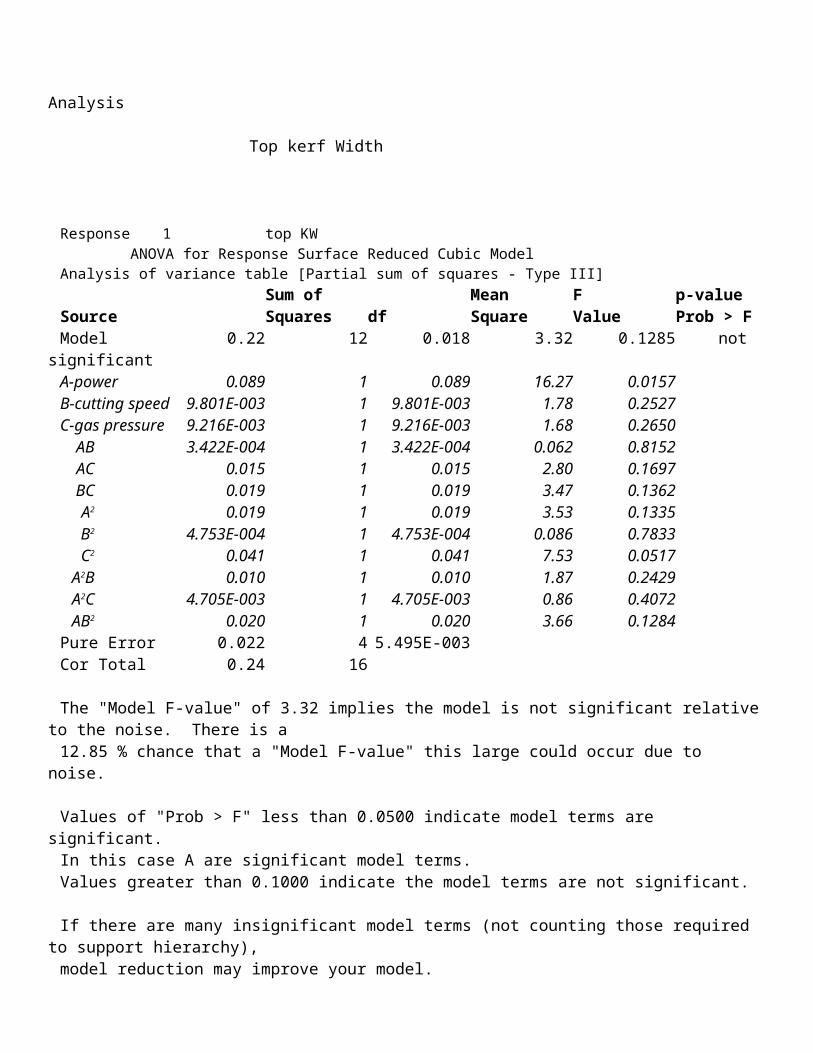
top KW0.773
0.3
X1 = A: powerX2 = B: cutting speed
Actual FactorC: gas pressure = 0.80
2000.00 2500.00
3000.00 3500.00
4000.00
3500.00
4000.00
4500.00
5000.00
5500.00
0.3
0.38
0.46
0.54
0.62
to
p K
W
A: pow er
B: cutting speed
Design-Expert® Software
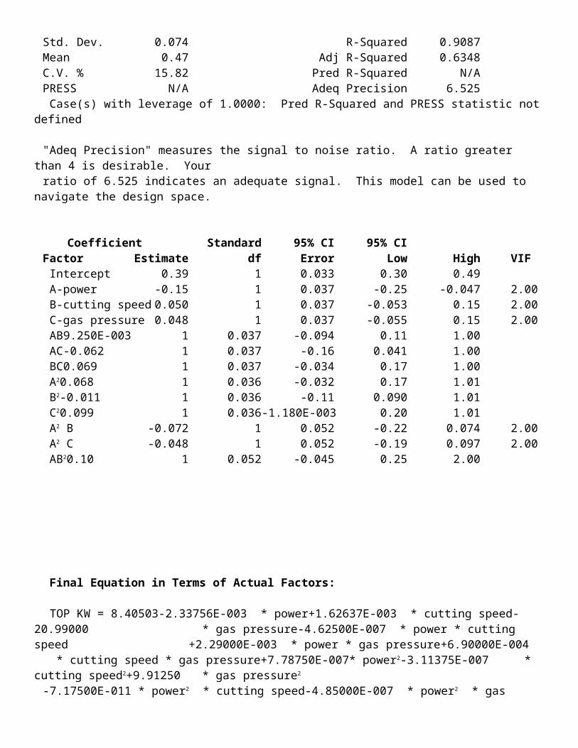
top KW0.773
0.3
X1 = A: powerX2 = C: gas pressure
Actual FactorB: cutting speed = 4500.00
2000.00 2500.00
3000.00 3500.00
4000.00
0.70
0.75
0.80
0.85
0.90
0.3
0.42
0.54
0.66
0.78
to
p K
W
A: pow er
C: gas pressure
Design-Expert® Software
top KW0.773
0.3
X1 = B: cutting speedX2 = C: gas pressure
Actual FactorA: power = 3000.00
3500.00 4000.00
4500.00 5000.00
5500.00
0.70
0.75
0.80
0.85
0.90
0.3
0.3875
0.475
0.5625
0.65
to
p K
W
B: cutting speed
C: gas pressure
Bottom Kerf Width
Response 2 bottom KW ANOVA for Response Surface Reduced Cubic ModelAnalysis of variance table [Partial sum of squares - Type III]
Sum of Mean F p-valueSource Squares df Square Value Prob > F
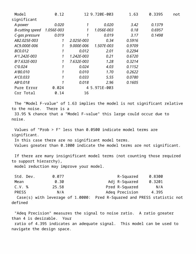
Model 0.12 12 9.720E-003 1.63 0.3395 not significant
A-power 0.020 1 0.020 3.42 0.1379B-cutting speed 1.056E-003 1 1.056E-003 0.18 0.6957C-gas pressure 0.019 1 0.019 3.17 0.1498AB2.025E-003 1 2.025E-003 0.34 0.5916AC9.000E-006 1 9.000E-006 1.507E-003 0.9709BC0.012 1 0.012 2.01 0.2294A21.242E-003 1 1.242E-003 0.21 0.6720B27.632E-003 1 7.632E-003 1.28 0.3214C20.024 1 0.024 4.03 0.1152A2B0.010 1 0.010 1.70 0.2622A2C0.033 1 0.033 5.55 0.0780AB20.018 1 0.018 2.96 0.1605Pure Error 0.024 4 5.971E-003Cor Total 0.14 16
The "Model F-value" of 1.63 implies the model is not significant relative to the noise. There is a33.95 % chance that a "Model F-value" this large could occur due to noise.
Values of "Prob > F" less than 0.0500 indicate model terms are significant. In this case there are no significant model terms. Values greater than 0.1000 indicate the model terms are not significant. If there are many insignificant model terms (not counting those required to support hierarchy), model reduction may improve your model.
Std. Dev. 0.077 R-Squared 0.8300Mean 0.30 Adj R-Squared 0.3201C.V. % 25.58 Pred R-Squared N/APRESS N/A Adeq Precision 4.395 Case(s) with leverage of 1.0000: Pred R-Squared and PRESS statistic not defined
"Adeq Precision" measures the signal to noise ratio. A ratio greater than 4 is desirable. Your ratio of 4.395 indicates an adequate signal. This model can be used to navigate the design space.
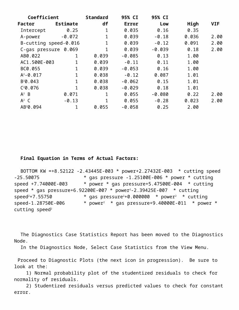
Coefficient Standard 95% CI 95% CIFactor Estimate df Error Low High VIF Intercept 0.25 1 0.035 0.16 0.35
A-power -0.072 1 0.039 -0.18 0.036 2.00 B-cutting speed -0.016 1 0.039 -0.12 0.091 2.00 C-gas pressure 0.069 1 0.039 -0.039 0.18 2.00 AB0.022 1 0.039 -0.085 0.13 1.00 AC1.500E-003 1 0.039 -0.11 0.11 1.00 BC0.055 1 0.039 -0.053 0.16 1.00 A2-0.017 1 0.038 -0.12 0.087 1.01 B20.043 1 0.038 -0.062 0.15 1.01 C20.076 1 0.038 -0.029 0.18 1.01 A2 B0.071 1 0.055 -0.080 0.22 2.00 A2 C-0.13 1 0.055 -0.28 0.023 2.00 AB20.094 1 0.055 -0.058 0.25 2.00
Final Equation in Terms of Actual Factors:
BOTTOM KW =+8.52122 -2.43445E-003 * power+2.27432E-003 * cutting speed -25.50075 * gas pressure -1.25100E-006 * power * cutting speed +7.74000E-003 * power * gas pressure+5.47500E-004 * cutting speed * gas pressure+6.92200E-007 * power2-2.39425E-007 * cutting speed2+7.55750 * gas pressure2+0.000000
* power2 * cutting speed-1.28750E-006 * power2 * gas pressure+9.40000E-011 * power * cutting speed2
The Diagnostics Case Statistics Report has been moved to the Diagnostics Node. In the Diagnostics Node, Select Case Statistics from the View Menu.
Proceed to Diagnostic Plots (the next icon in progression). Be sure to look at the: 1) Normal probability plot of the studentized residuals to check for normality of residuals. 2) Studentized residuals versus predicted values to check for constant error. 3) Externally Studentized Residuals to look for outliers, i.e., influential values. 4) Box-Cox plot for power transformations.
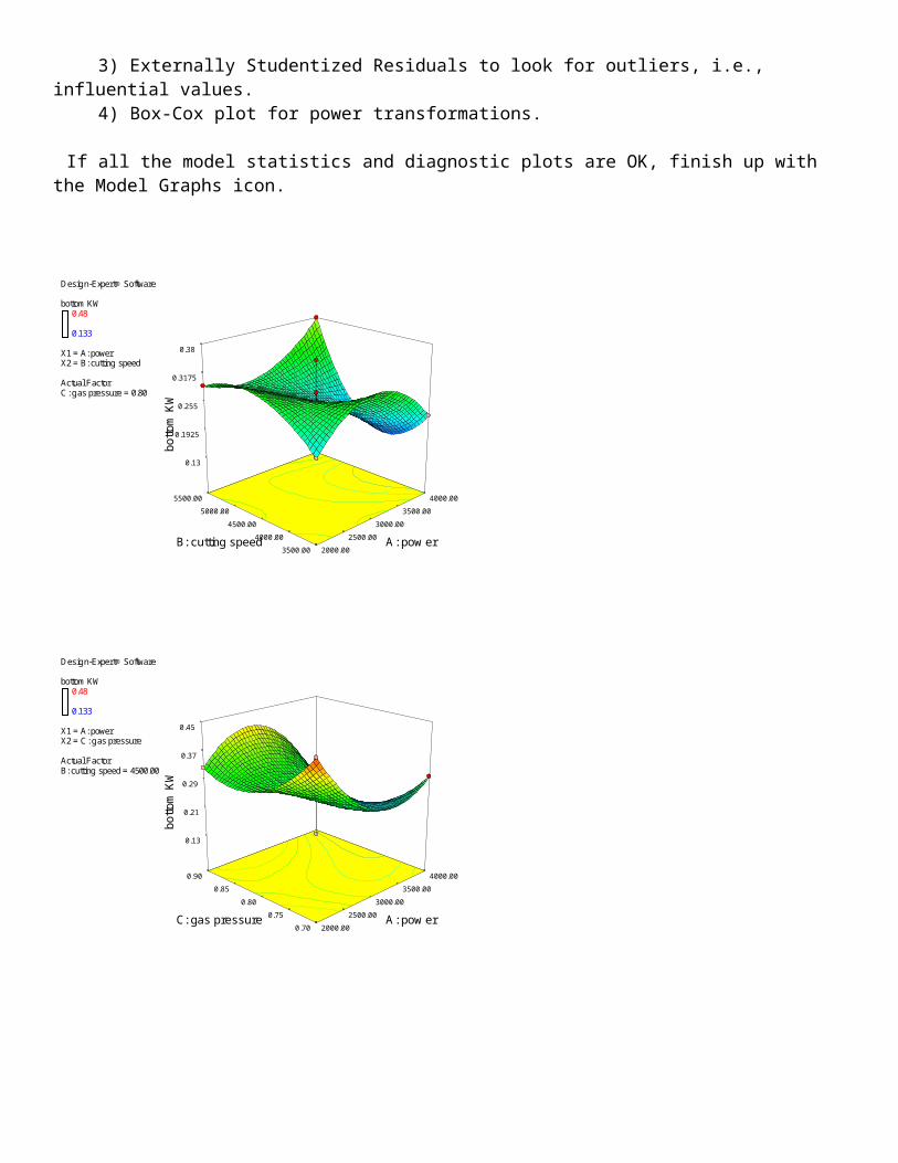
If all the model statistics and diagnostic plots are OK, finish up with the Model Graphs icon.
Design-Expert® Software
bottom KW0.48
0.133
X1 = A: powerX2 = B: cutting speed
Actual FactorC: gas pressure = 0.80
2000.00
2500.00
3000.00
3500.00
4000.00
3500.00
4000.00
4500.00
5000.00
5500.00
0.13
0.1925
0.255
0.3175
0.38
b
ott
om
KW
A: pow er B: cutting speed
Design-Expert® Software
bottom KW0.48
0.133
X1 = A: powerX2 = C: gas pressure
Actual FactorB: cutting speed = 4500.00
2000.00
2500.00
3000.00
3500.00
4000.00
0.70
0.75
0.80
0.85
0.90
0.13
0.21
0.29
0.37
0.45
b
ott
om
KW
A: pow er C: gas pressure
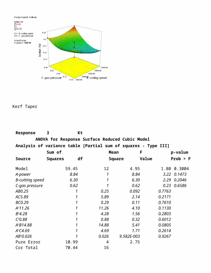
Design-Expert® Software
bottom KW0.48
0.133
X1 = B: cutting speedX2 = C: gas pressure
Actual FactorA: power = 3000.00
3500.00
4000.00
4500.00
5000.00
5500.00
0.70
0.75
0.80
0.85
0.90
0.13
0.22
0.31
0.4
0.49
b
ott
om
KW
B: cutting speed C: gas pressure
Kerf Taper
Response 3 Kt ANOVA for Response Surface Reduced Cubic ModelAnalysis of variance table [Partial sum of squares - Type III]
Sum of Mean F p-valueSource Squares df Square Value Prob > F
Model 59.45 12 4.95 1.80 0.3004A-power 8.84 1 8.84 3.22 0.1473B-cutting speed 6.30 1 6.30 2.29 0.2046C-gas pressure 0.62 1 0.62 0.23 0.6586AB0.25 1 0.25 0.092 0.7763AC5.89 1 5.89 2.14 0.2171BC0.29 1 0.29 0.11 0.7610A211.26 1 11.26 4.10 0.1130B24.28 1 4.28 1.56 0.2803C20.88 1 0.88 0.32 0.6012A2B14.88 1 14.88 5.41 0.0805A2C4.69 1 4.69 1.71 0.2614AB20.026 1 0.026 9.582E-003 0.9267Pure Error 10.99 4 2.75Cor Total 70.44 16
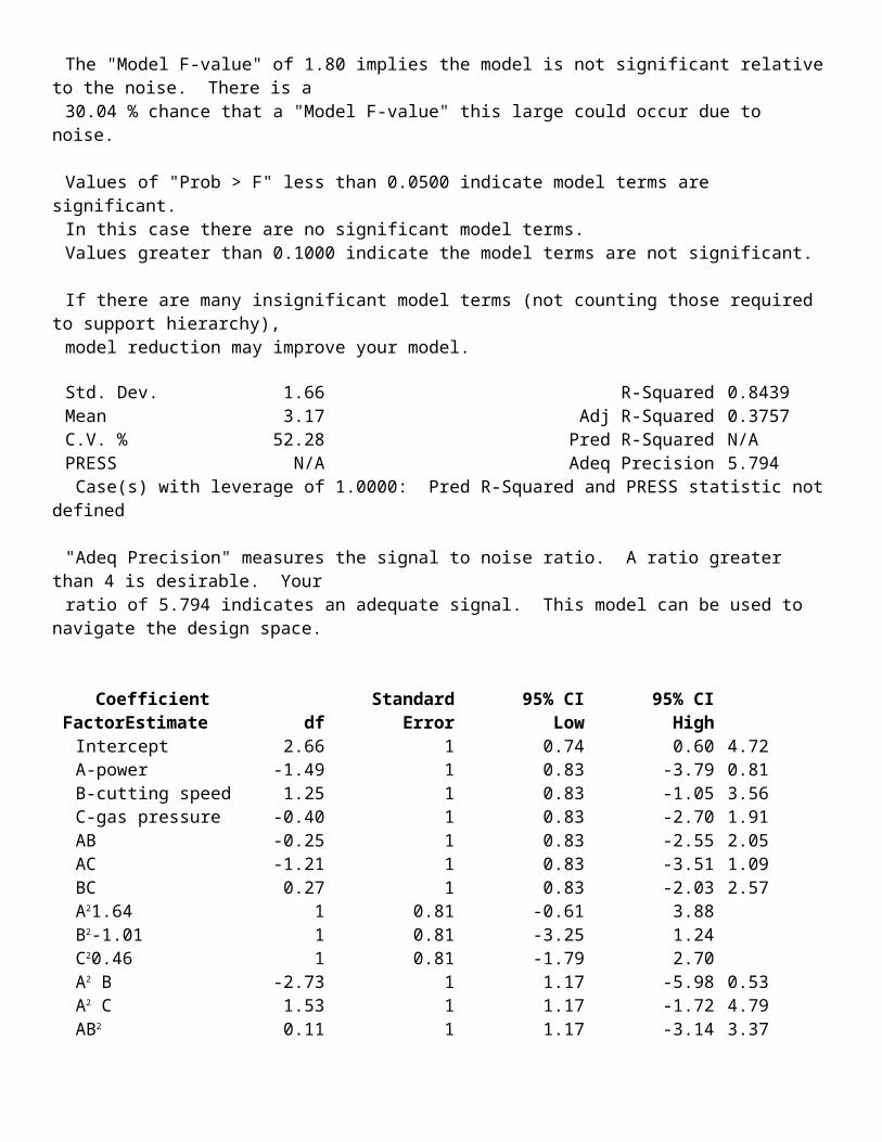
The "Model F-value" of 1.80 implies the model is not significant relative to the noise. There is a30.04 % chance that a "Model F-value" this large could occur due to noise.
Values of "Prob > F" less than 0.0500 indicate model terms are significant. In this case there are no significant model terms. Values greater than 0.1000 indicate the model terms are not significant.
If there are many insignificant model terms (not counting those required to support hierarchy), model reduction may improve your model.
Std. Dev. 1.66 R-Squared 0.8439Mean 3.17 Adj R-Squared 0.3757C.V. % 52.28 Pred R-Squared N/APRESS N/A Adeq Precision 5.794 Case(s) with leverage of 1.0000: Pred R-Squared and PRESS statistic not defined
"Adeq Precision" measures the signal to noise ratio. A ratio greater than 4 is desirable. Your ratio of 5.794 indicates an adequate signal. This model can be used to navigate the design space.
Coefficient Standard 95% CI 95% CI Factor Estimate df Error Low High
Intercept 2.66 1 0.74 0.60 4.72 A-power -1.49 1 0.83 -3.79 0.81 B-cutting speed 1.25 1 0.83 -1.05 3.56 C-gas pressure -0.40 1 0.83 -2.70 1.91 AB-0.25 1 0.83 -2.55 2.05 AC-1.21 1 0.83 -3.51 1.09 BC0.27 1 0.83 -2.03 2.57 A21.64 1 0.81 -0.61 3.88 B2-1.01 1 0.81 -3.25 1.24 C20.46 1 0.81 -1.79 2.70 A2 B -2.73 1 1.17 -5.98 0.53 A2 C 1.53 1 1.17 -1.72 4.79 AB2 0.11 1 1.17 -3.14 3.37
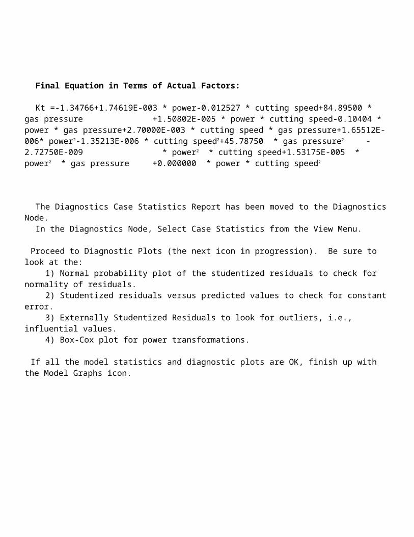
Final Equation in Terms of Actual Factors:
Kt =-1.34766+1.74619E-003 * power-0.012527 * cutting speed+84.89500 * gas pressure+1.50802E-005 * power * cutting speed-0.10404 * power * gas pressure+2.70000E-003 * cutting speed * gas pressure+1.65512E-006* power2-1.35213E-006 * cutting speed2+45.78750 * gas pressure2-2.72750E-009
* power2 * cutting speed+1.53175E-005 * power2 * gas pressure+0.000000 * power * cutting speed2
The Diagnostics Case Statistics Report has been moved to the Diagnostics Node. In the Diagnostics Node, Select Case Statistics from the View Menu.
Proceed to Diagnostic Plots (the next icon in progression). Be sure to look at the: 1) Normal probability plot of the studentized residuals to check for normality of residuals. 2) Studentized residuals versus predicted values to check for constant error. 3) Externally Studentized Residuals to look for outliers, i.e., influential values. 4) Box-Cox plot for power transformations.
If all the model statistics and diagnostic plots are OK, finish up with the Model Graphs icon.
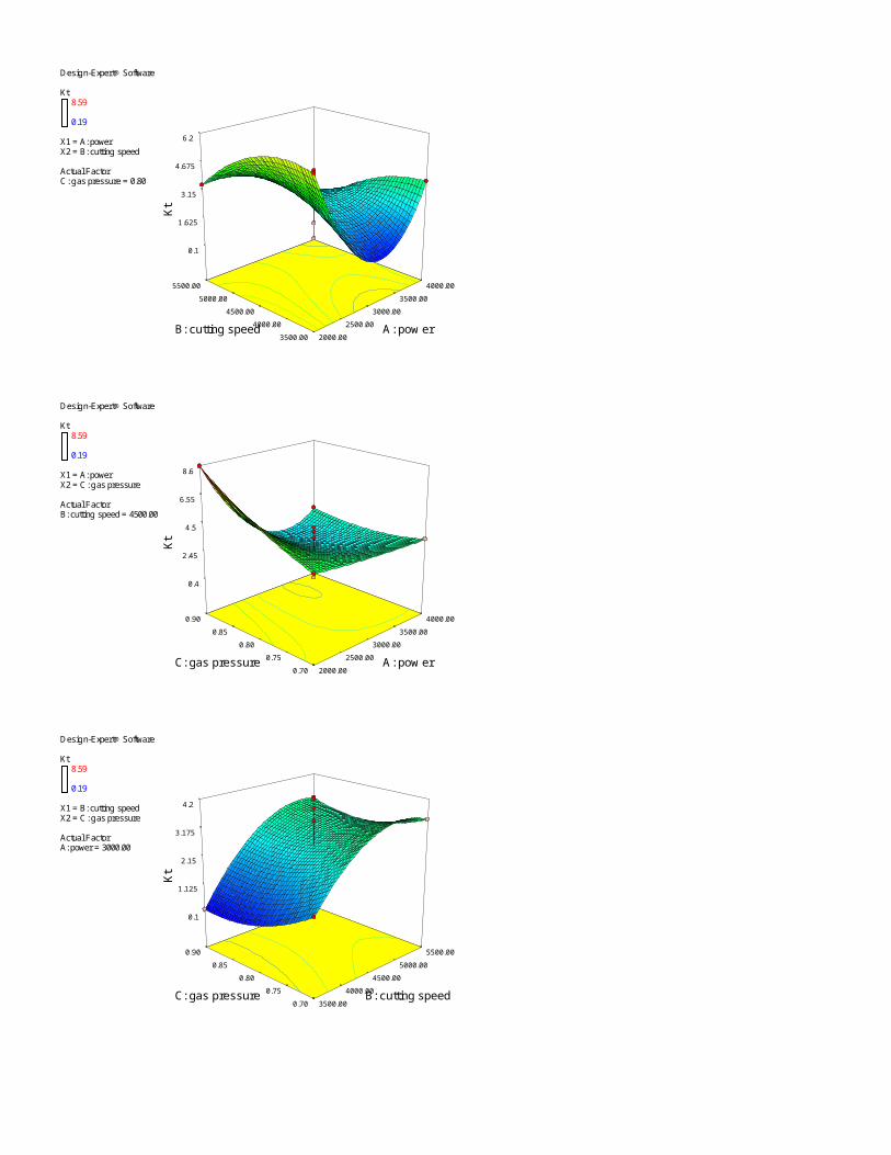
Design-Expert® Software
Kt8.59
0.19
X1 = A: powerX2 = B: cutting speed
Actual FactorC: gas pressure = 0.80
2000.00
2500.00
3000.00
3500.00
4000.00
3500.00
4000.00
4500.00
5000.00
5500.00
0.1
1.625
3.15
4.675
6.2
K
t
A: pow er B: cutting speed
Design-Expert® Software
Kt8.59
0.19
X1 = A: powerX2 = C: gas pressure
Actual FactorB: cutting speed = 4500.00
2000.00
2500.00
3000.00
3500.00
4000.00
0.70
0.75
0.80
0.85
0.90
0.4
2.45
4.5
6.55
8.6
K
t
A: pow er C: gas pressure
Design-Expert® Software
Kt8.59
0.19
X1 = B: cutting speedX2 = C: gas pressure
Actual FactorA: power = 3000.00
3500.00
4000.00
4500.00
5000.00
5500.00
0.70
0.75
0.80
0.85
0.90
0.1
1.125
2.15
3.175
4.2
K
t
B: cutting speed C: gas pressure
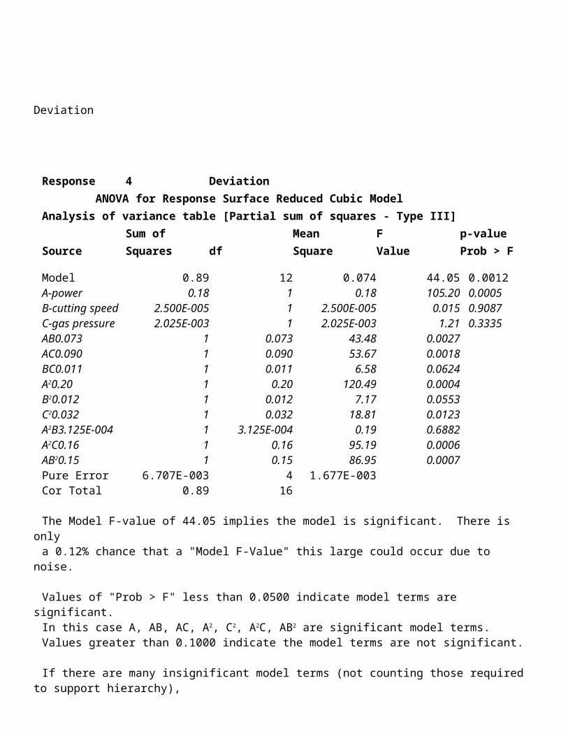
Deviation
Response 4 Deviation ANOVA for Response Surface Reduced Cubic ModelAnalysis of variance table [Partial sum of squares - Type III]
Sum of Mean F p-valueSource Squares df Square Value Prob > F
Model 0.89 12 0.074 44.05 0.0012A-power 0.18 1 0.18 105.20 0.0005B-cutting speed 2.500E-005 1 2.500E-005 0.015 0.9087C-gas pressure 2.025E-003 1 2.025E-003 1.21 0.3335AB0.073 1 0.073 43.48 0.0027AC0.090 1 0.090 53.67 0.0018BC0.011 1 0.011 6.58 0.0624A20.20 1 0.20 120.49 0.0004B20.012 1 0.012 7.17 0.0553C20.032 1 0.032 18.81 0.0123A2B3.125E-004 1 3.125E-004 0.19 0.6882A2C0.16 1 0.16 95.19 0.0006AB20.15 1 0.15 86.95 0.0007Pure Error 6.707E-003 4 1.677E-003Cor Total 0.89 16
The Model F-value of 44.05 implies the model is significant. There is only
a 0.12% chance that a "Model F-Value" this large could occur due to noise.
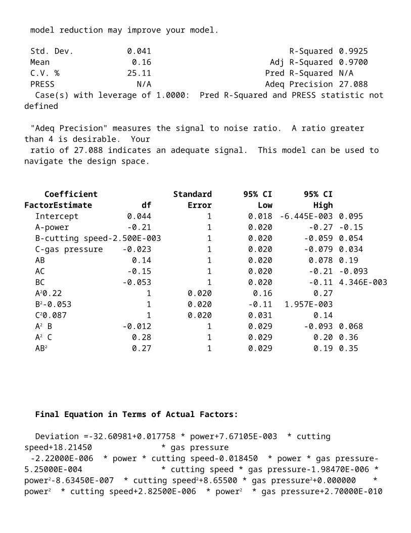
Values of "Prob > F" less than 0.0500 indicate model terms are significant. In this case A, AB, AC, A2, C2, A2C, AB2 are significant model terms. Values greater than 0.1000 indicate the model terms are not significant. If there are many insignificant model terms (not counting those required to support hierarchy), model reduction may improve your model.
Std. Dev. 0.041 R-Squared 0.9925Mean 0.16 Adj R-Squared 0.9700C.V. % 25.11 Pred R-Squared N/APRESS N/A Adeq Precision 27.088 Case(s) with leverage of 1.0000: Pred R-Squared and PRESS statistic not defined
"Adeq Precision" measures the signal to noise ratio. A ratio greater than 4 is desirable. Your ratio of 27.088 indicates an adequate signal. This model can be used to navigate the design space.
Coefficient Standard 95% CI 95% CIFactor Estimate df Error Low High
Intercept 0.044 1 0.018 -6.445E-003 0.095 A-power -0.21 1 0.020 -0.27 -0.15 B-cutting speed -2.500E-003 1 0.020 -0.059 0.054 C-gas pressure -0.023 1 0.020 -0.079 0.034 AB0.14 1 0.020 0.078 0.19 AC-0.15 1 0.020 -0.21 -0.093 BC-0.053 1 0.020 -0.11 4.346E-003 A20.22 1 0.020 0.16 0.27 B2-0.053 1 0.020 -0.11 1.957E-003 C20.087 1 0.020 0.031 0.14 A2 B -0.012 1 0.029 -0.093 0.068 A2 C 0.28 1 0.029 0.20 0.36 AB2 0.27 1 0.029 0.19 0.35
Final Equation in Terms of Actual Factors:
Deviation =-32.60981+0.017758 * power+7.67105E-003 * cutting speed+18.21450 * gas pressure-2.22000E-006 * power * cutting speed-0.018450 * power * gas pressure-5.25000E-004 * cutting speed *
gas pressure-1.98470E-006 * power2-8.63450E-007 * cutting speed2+8.65500 * gas pressure2+0.000000 * power2 * cutting speed+2.82500E-006 * power2 * gas pressure+2.70000E-010 * power * cutting speed2
The Diagnostics Case Statistics Report has been moved to the Diagnostics Node. In the Diagnostics Node, Select Case Statistics from the View Menu.
Proceed to Diagnostic Plots (the next icon in progression). Be sure to look at the: 1) Normal probability plot of the studentized residuals to check for normality of residuals.
2) Studentized residuals versus predicted values to check for constant error. 3) Externally Studentized Residuals to look for outliers, i.e., influential values. 4) Box-Cox plot for power transformations.
If all the model statistics and diagnostic plots are OK, finish up with the Model Graphs icon.
Design-Expert® Software
Deviation0.97
0
X1 = A: powerX2 = B: cutting speed
Actual FactorC: gas pressure = 0.80
2000.00
2500.00
3000.00
3500.00
4000.00
3500.00
4000.00
4500.00
5000.00
5500.00
-0.06
0.08
0.22
0.36
0.5
D
evi
atio
n
A: pow er B: cutting speed
Design-Expert® Software
Deviation0.97
0
X1 = A: powerX2 = C: gas pressure
Actual FactorB: cutting speed = 4500.00
2000.00 2500.00
3000.00 3500.00
4000.00
0.70
0.75
0.80
0.85
0.90
-0.01
0.2375
0.485
0.7325
0.98
D
evi
atio
n
A: pow er
C: gas pressure
Design-Expert® Software
Deviation0.97
0
X1 = B: cutting speedX2 = C: gas pressure
Actual FactorA: power = 3000.00
3500.00
4000.00
4500.00
5000.00
5500.00
0.70
0.75
0.80
0.85
0.90
-0.03
0.02
0.07
0.12
0.17
D
evi
atio
n
B: cutting speed C: gas pressure