project 3.5 aggregated load shedding task 3.5.5 analysis...
TRANSCRIPT

Project 3.5
Aggregated Load Shedding
Task 3.5.5
Analysis and Field Test of Semi-Automated Load Shedding
in LA County Test Buildings
Deliverable 3.5.5(a)
Report of Field Testing
Submitted to Architectural Energy Corporation
Under the
California Energy Commission’s
Public Interest Energy Research (PIER) Program
Energy-Efficient and Affordable
Small Commercial and Residential Buildings
California Energy Commission Contract 400-99-011
P.R. Armstrong and L.K. Norford
Massachusetts Institute of Technology May 29, 2003 Revised , 2003

nilm\reports\MITReport355a5.doc ii/57 2006-01-28 11:12
ii
Table of Contents Introduction 1 Technical Approach 3
Curtailment strategies 3 Peak-shifting strategies 4 Instrumentation 6 Envelope thermal response 8 Model identification 11 Peak-shifting potential 12 Curtailment tests 12 Peak-shifting tests 13
Outcomes 14 ECC Curtailment 14 ISD curtailment 15 Zone conditions 16 ECC peak-shifting 17 ISD peak shifting 19 Model identification 22 Peak-shifting potential 25
Conclusions and Recommendations 28 References 30 Appendix A. ISD Building Description 31 Appendix B. ECC Building Description 37 Appendix C. Model Identification Algorithm and Tests 42 Appendix D. Design Conditions and TMY Weather 44 Appendix E. Simulation 45 Appendix F. Electric Rate Structure 51 Appendix G. Optimization Algorithms 53
nilm\reports\MITReport355a5.doc 1/57 2006-01-28 11:12
1
Report on Measurement and Experimental Plans for Load Shedding in LA County Buildings THIS REPORT WAS PREPARED AS A RESULT OF WORK SPONSORED BY THE CALIFORNIA ENERGY COMMISSION (COMMISSION). IT DOES NOT NECESSARILY REPRESENT THE VIEWS OF THE COMMISSION, ITS EMPLOYEES, OR THE STATE OF CALIFORNIA. THE COMMISSION, THE STATE OF CALIFORNIA, ITS EMPLOYEES, CONTRACTORS, AND SUBCONTRACTORS MAKE NO WARRANTY, EXPRESS OR IMPLIED, AND ASSUME NO LEGAL LIABILITY FOR THE INFORMATION IN THIS REPORT; NOR DOES ANY PARTY REPRESENT THAT THE USE OF THIS INFORMATION WILL NOT INFRINGE UPON PRIVATELY OWNED RIGHTS. THIS REPORT HAS NOT BEEN APPROVED OR DISAPPROVED BY THE COMMISSION NOR HAS THE COMMISSION PASSED UPON THE ACCURACY OR ADEQUACY OF THE INFORMATION IN THIS REPORT.
Introduction This report documents the load shedding control strategy development and the field test activities of CEC/AEC Task 3.5.5. The body of the report describes load curtailment strategies, instrumentation, and the results of simulations and field tests. The objectives of the load control task are threefold:
1) characterize transient building cooling load models empirically, 2) identify load shedding potential and promising control strategies, 3) demonstrate the resulting load shedding controls in our test buildings, 4) assess the broader potential for peak shifting in LA.
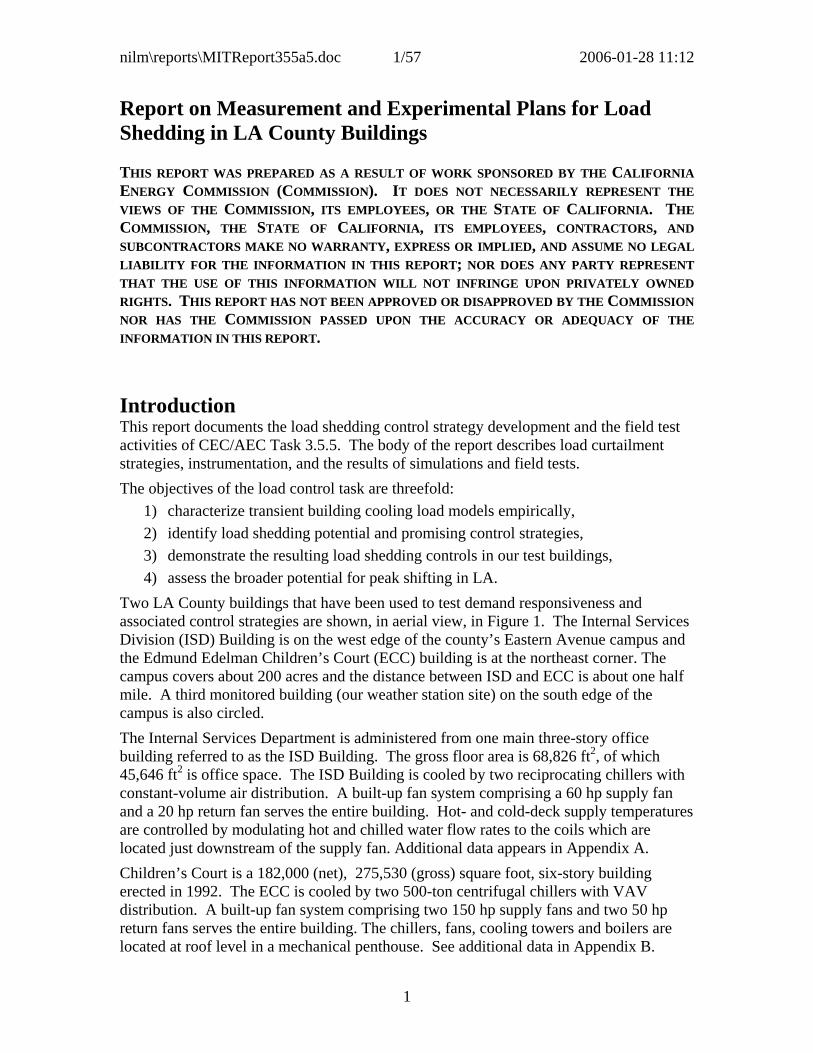
Two LA County buildings that have been used to test demand responsiveness and associated control strategies are shown, in aerial view, in Figure 1. The Internal Services Division (ISD) Building is on the west edge of the county’s Eastern Avenue campus and the Edmund Edelman Children’s Court (ECC) building is at the northeast corner. The campus covers about 200 acres and the distance between ISD and ECC is about one half mile. A third monitored building (our weather station site) on the south edge of the campus is also circled. The Internal Services Department is administered from one main three-story office building referred to as the ISD Building. The gross floor area is 68,826 ft2, of which 45,646 ft2 is office space. The ISD Building is cooled by two reciprocating chillers with constant-volume air distribution. A built-up fan system comprising a 60 hp supply fan and a 20 hp return fan serves the entire building. Hot- and cold-deck supply temperatures are controlled by modulating hot and chilled water flow rates to the coils which are located just downstream of the supply fan. Additional data appears in Appendix A. Children’s Court is a 182,000 (net), 275,530 (gross) square foot, six-story building erected in 1992. The ECC is cooled by two 500-ton centrifugal chillers with VAV distribution. A built-up fan system comprising two 150 hp supply fans and two 50 hp return fans serves the entire building. The chillers, fans, cooling towers and boilers are located at roof level in a mechanical penthouse. See additional data in Appendix B.

nilm\reports\MITReport355a5.doc 2/57 2006-01-28 11:12
2
Figure 1. Monitored buildings on the LA County Eastern Avenue Campus
Because they are located on the same campus, coordination of load shedding among the buildings should be possible. Coordination is important for achieving the best outcomes with respect to County utility costs and electric supply reliability at a regional level. The County recently installed a Cutler-Hammer monitoring system that allows operators to track over 200 service entrance and (in some cases) significant end-use loads in most of the large county buildings on and off the Eastern Avenue campus. Fifteen-minute load data are collected and disseminated by a Silicon Energy data management system so that the data can be readily accessed by staff for a variety of analyses including, potentially, the coordination of operator responses to a utility curtailment.
The body of the report has two main sections: Technical Approach and Outcomes. Each of these main sections is subdivided by subtask: Control strategy development, Instrumentation, Thermal response model, Model identification, Benefits assessment, and Field testing. Appendix A and B document the characteristics of the two test buildings. Appendix C documents the model identification code. Appendices D-G pertain to benefits assessment: Appendix D summarizes climate data, Appendix E describes the main elements of the simulation program, Appendix F describes the electric rate structure and evaluation of annual electric utility costs for a given building, and Appendix G describes the night precooling optimal control algorithms.

nilm\reports\MITReport355a5.doc 3/57 2006-01-28 11:12
3
Technical Approach Load shedding and peak shifting strategies are constrained by building and HVAC plant characteristics as well as climate, utility rate structure and building occupancy requirements. The analytical framework for dealing with different climates, rate structures and occupancies is well established. One-day ahead weather forecasts are now quite reliable and internal gains, predominantly light and plug loads, can, once disaggregated by a NILM from the building total, be similarly predicted [Seem and Braun 1991]. However, thermal response to weather, internal loads and HVAC inputs is generally considered unique to each building and difficult to characterize empirically [Braun and Chaturvedi 2002]. The development of a general model and model identification procedure sufficiently robust to be automated is therefore a central and challenging prerequisite to the implementation of useful control strategies. The need to test the model and identification procedure, as well as the control strategies, in at least two very different buildings follows from recognition that different buildings are unique with respect to thermal response. Careful instrumentation and monitoring of the test buildings is essential to the experimental side of this task. Broader assessment of control strategies, on the other hand, can only be accomplished by simulation. A simulation model that can handle empirically derived building thermal response functions as well as engineering models is therefore another key part of the technical approach. Curtailment Strategies. A building’s peak electrical demand may be reduced by
1) reducing non-HVAC loads (lighting and plug loads), and/or 2) reducing HVAC cooling capacity (fans, chillers, pumps and cooling tower).
Reduction of base load is the first measure that should be considered because energy savings accrue for all hours of operation, are not subject to occupant, operator, or controller behaviors, and generally result in additional cooling plant and distribution system load reductions. Lighting is a significant base-load component in ISD, ECC, and most other county buildings. Office equipment is a significant base load in the ISD and ECC and other types of equipment may be significant in other county buildings. Improvements in heating and cooling plant and air distribution efficiency are also classified as baseload reduction measures1. Short-term reductions in plug and lighting loads are generally the second most desirable curtailment measure because they produce additional cooling capacity reductions without occupant discomfort. The bonus, of course, is that curtailment of lighting and plug loads effects an immediate reduction in cooling load which the control system will sense and automatically respond to by effecting just the capacity reduction needed to maintain room conditions near setpoint. Dispatchable loads may include such equipment as copiers and printers, two-level lighting, general lighting (if task lighting or centrally controlled dimmable ballasts are available) or even task lighting (if sufficient daylighting is available), and may even be extended to workstations of users who are able to indulge in
1 The ISD has significant potential in the form of CV to VAV conversion and chiller stage sequencing. ECC improvements include static pressure reset, variable speed pumps, and replacement of the currently broken chiller#2 by a smaller chiller with good part load efficiency at low lift temperatures.

nilm\reports\MITReport355a5.doc 4/57 2006-01-28 11:12
4
non-computer-related work without undue disruption of their productivity. Many of these additional reductions would be controlled manually. Occupants could be notified by email, phone broadcast, or over a public address system. Some advance training and periodic "fire drills" will be necessary in most situations to implement this sort of curtailment strategy effectively. The ability to measure the response during such occupant-implemented load curtailment may be key to its effectiveness. A third curtailment measure that can be implemented involves further reduction in cooling capacity, either by direct control or by raising room temperature (and humidity, if implemented) set points. The setpoint changes can be abrupt or gradual, depending on the curtailment response desired. The occupants will experience loss of comfort in either case, and the amount of additional capacity reduction, and its duration, will be limited by occupants’ tolerances for elevated temperature and humidity levels. The fourth, and most difficult, curtailment measure requires control functions that anticipate curtailment by anywhere from one to sixteen hours, and increase cooling capacity modestly during this pre-curtailment period so that zone conditions are as cold and dry as can be tolerated immediately before the curtailment period and the thermal masses of building structure and contents are at or even below this minimum tolerable temperature. With such a favorable initial state, the reduction in cooling capacity and its duration can be made significantly larger—i.e., the amount of cooling capacity that can be shed during the curtailment event is significantly increased. There are at least three distinct schemes for implementing the fourth (precooling) measure as a retrofit:
1) Night cooling (outside air with or without chiller operation) 2) Extended period of reduced setpoint (starting the day with a lower setpoint or
ramping it down gradually during the pre-curtailment period) 3) Short period of reduced setpoint before the anticipated load shedding time2.
Peak Shifting Strategies. Curtailment is a short-term mechanism to prevent aggregate load from exceeding generation capacity. Curtailment programs usually provide no direct incentive for efficient operation. Utilities have used (extensively in the last two decades) demand- and time-of-use- (TOU) based rate structures, on the other hand, to provide longer-term limits on peak loads3. Peak-shifting is a customer response that typically benefits both the utility and the customer under a time-of-use- or simple demand-based rate structure4. The incentive to improve energy efficiency, although often ignored by cream skimming measures, does exist under TOU rates. Night cooling is a peak shifting strategy that is well suited to office buildings and similar air-conditioned buildings in climates where cool nights and significant daytime cooling loads coincide through much of the year. Night cooling can save energy by using
2 For lunch-hour precooling to be most effective, occupants should be trained to turn off lights and other unnecessary equipment before going out—at least on days when curtailment can be anticipated. If base-load is not so reduced, a new building peak load may result. Moreover, if many buildings were to adopt lunch-hour precooling, the utility peak might actually be shifted from mid-afternoon to the lunch hour. 3 for which a utility typically incurs higher costs of generation, T&D, and risk of service interruption. 4 “Real-time” pricing with 24 hour advance rate notification is another effective rate structure that has been tested, and appears to have an assured future, in electric utility markets.

nilm\reports\MITReport355a5.doc 5/57 2006-01-28 11:12
5
ambient conditions (cool night air) to remove heat from the building structure and contents or by using forms of mechanical cooling that are particularly efficient under night cooling (low lift, small load) conditions. The maximum usable cooling capacity stored on a given day is proportional to the normal zone cooling setpoint minus the thermal capacitance weighted average of contents and structure temperatures at the start of occupancy. The actual capacity is roughly (but not exactly, because the envelope temperature field is affected by outdoor, as well as indoor, conditions) proportional to the change in the thermal-capacitance-weighted average of contents and structure temperatures between start and end of occupancy. Stored capacity is limited in four ways: total thermal capacitance, rate of charge/discharge, night temperature, and comfort constraints. Within the framework of these basic limitations, however, there are a number of control strategies that can be used to implement night cooling. Constant Volume(CV) Precooling. The simplest strategy is to cool the building at night whenever outdoor temperature is below return air temperature and to modulate the cooling rate to just maintain the minimum comfortable temperature (MCT) until occupancy. On warm nights there may be no cooling, on mild nights the minimum comfortable temperature may not be reached. This strategy is suboptimal for two reasons: no part of the mass can ever be cooled below the MCT and the cost of fan energy has not been considered. CV Delayed Start. The simple strategy can be improved by running the fan fewer hours at night. The objective in this strategy is to reach the MCT not too long before occupancy and, on days with little cooling load, to not reach MCT. Implementation is relatively simple because there is only one variable, start time, to be determined each night. CV Subcooling/Tempering. Delayed start is still not optimal because the potential to cool part of the mass below MCT is not exploited. A third CV strategy, therefore, add another variable, the tempering time. With this strategy the optimal night cooling start and stop times are determined each day. Constant Volume Objective Function. The foregoing strategies have been described in terms of mass state at start of occupancy. However this state is not observable and, in any case, is only indirectly related to the objectives of minimizing plant demand and energy costs. An objective function that represents daily electricity cost will therefore be used. For the most elaborate CV strategy, daily cost can be minimized by enumerating all possible start and tempering times and comparing total daily cost for each5. Variable Volume Precooling. The fan energy required on any given day can be further reduced by modulating fan speed during the night cooling phase. This is a much more difficult optimization problem because any sense in which daily cost is monotonic with fan speed in a given hour is lost. Two approaches will be used to make the problem tractable: discretization of fan speed and application of a fan modulating function in
5 In practice, a one hour time step is convenient and reasonable in terms of control resolution. Also, complete enumeration is found to be unnecessary. One starts with the earliest start time and shortest (zero) tempering time. Tempering time is increased until daily cost stops decreasing. The process is repeated with progressively later start times until the daily cost stops decreasing with lateness of start time.

nilm\reports\MITReport355a5.doc 6/57 2006-01-28 11:12
6
which gain is determined daily by optimizations analogous to the CV-delayed-start and CV-tempering strategies. The thermal response of the envelope and contents is embedded in the objective function. It is important that the thermal response function represent the building being controlled. A key result of this task is a robust method of obtaining the appropriate model based on actual thermal response as measured by, e.g., the HVAC control system and NILMs installed at the service entrance and HVAC subpanel. The technical approaches for characterizing envelope thermal response and for assessing the potential for curtailment and night precooling are developed after a brief digression on instrumentation of the test buildings. Instrumentation. Two NILM installations were made in each building, one to track HVAC (chillers, fans, pumps), the other to track whole building (lighting, plugs, other non-HVAC) loads. Each NILM, except at the ECC service entrance, is shadowed by a K20-6 (traditional end-use metering) logger with one-minute integration intervals. The K20-6 loggers serve to monitor the non-power variables needed to properly control load shedding activity and analyze the effectiveness and comfort impacts of such actions6 as well as to verify NILM end-use disaggregation. One K20-6 logger can monitor 16 end-use circuits, 16 status or pulse channels, and 15 analog channels. The electrical end-use channels are documented in Appenices A and B. Return air temperature and humidity are measured in each building to provide an estimate of average zone conditions. The return temperature is typically a biased estimate7 of average zone temperature when zone air returns through ceiling plenums because most of the heat from lights is added to the air as or after it enters the ceiling plenum. Room temperatures in selected zones (Tables 1 and 2) are monitored by unobtrusive battery-powered microloggers. The loggers sample temperature at 2 Hz and the sample averages are recorded at 5-minute intervals. Data storage capacity is 24 days; data are retrieved as needed to characterize envelope response and assess test results. Coil air-side temperature rise is measured in the ISD hot and cold decks and net air-handler temperature rise is measured in ECC. (Installation at the ECC chilled water coil was impractical because of the very large size (~12’ x 36’) of the coil face). Air-side temperature differences, measured by a thermopile with multiple upstream and downstream junctions distributed over the projected coil face area, determine sensible cooling capacity . The thermopile puts out a very low level signal (about 50 uV per Kelvin per pair of junctions) that is amplified by an auto-zeroing op-amp configured for the appropriate gain (200 to 2000 depending on the number of junction pairs in the
6 The variables needed for control, including end-use loads output by a NILM, would normally be monitored by the control system. Prototype NILMs may be interfaced to control systems in one or more of the project sites after the effectiveness of load shedding has been demonstrated. However, for the initial tests control and monitoring of load shedding actions and responses will be implemented independently. 7 The ideal sensor measures what the occupant perceives, Tocc, which is a weighted average from head to toe at whatever location the occupant chooses to occupy at a given time. A single fixed sensor can only provide an estimate, Tsense, of occupant-percieved temperature. In the most general linear model Tocc = Cox + Dou and Tsense = Csx + Dsu. These relations show that there is at least the possibility of obtaining a better estimate of Tocc from Tsense via a state observer.

nilm\reports\MITReport355a5.doc 7/57 2006-01-28 11:12
7
thermopile and the maximum temperature difference expected). The op-amp output is connected to a K20-6 analog input channel. (K20-6 input range is fixed at 0 to 5V). Table 1. ISD zone temperature micro-logger locations: Floor Wing Side Dept. Room Serial No Comment 0 S Core 522639 Mid open office; lost after 2003.01.241 N Core 332632 Mid open office 1 S Core 495219 Mid open office, Ron’s cubicle 2 N E 332635 Private office 2 N Core 495190 On T-stat outside west private office 2 S W 495213 Private office, Susan Lopez 2 S Core 522646 Mid open office 3 S Core 522644
500862 Mid open office, replaced 2002.06.26
Table 2. ECC zone temperature micro-logger locations: Floor Wing Side Dept. Room Serial No Comment G N core 0101 332630 sheriff (reception and open office) L N core 495205 large open office 2 N W 2700 495199 large open office near phone closet
T2N4 2 E N 332268 large private office (Jo Schiff) 3 E core 406 332633 court room converted to arts & crafts 3 N core 3511 522461 4 E S 400C 522645 four-person office (Angela Smith) 4 N core 417 522637 courtroom 5 E core 421 522640 courtroom (Judge John L.Henning) 5 C S Hall 522638 on T-stat near copy machine &
stairwell 5 N core 424 332631 courtroom 6 N 522643 three-person office and reception
(Lisa Romero/Ann Fragraso)
Boiler run times at each firing stage are monitored by installing relays in parallel with the boiler gas valves. The relays provide contact closure inputs to the K20-6 loggers that monitor thermal loads in each building. Note that boiler run time is the primary measure of heat supply in buildings with reheat coils (ECC) and is a redundant measure in buildings with central heating coils (ISD). The temperature and relative humidity (RH) of return, mixed and supply air are monitored by RTDs and HyCal RH sensors in the ECC. Weather is monitored at the Communications building. Outdoor temperature is measured by an RTD mounted in a radiation shield and solar radiation is measured by a LiCor pyranometer mounted on the wind cross-arm. Wind is measured by a 3-cup anemometer and an active (op-amp-based) rectifier to convert the AM signal to dc. Barometric pressure is measured by a Setra 207. Direct and diffuse components of solar radiation are determined by a shadowband pyranometer employing a LiCor model PY-200 detector and controlled by a CR10 logger.

nilm\reports\MITReport355a5.doc 8/57 2006-01-28 11:12
8
Characterize Envelope Thermal Response. Heat transfer and storage in the building structure and contents is governed by the diffusion equation
pckwhere
DxT
tT
DTtT
ρα
α
α
=
−∂∂
=∂∂
−∇=∂∂
)1(
)3(
2
2
2
(1)
In steady-state, one-dimensional diffusion, the second space derivative must be zero because the first time derivative is zero. But the first space derivative is a constant given by Fourier’s law:
)1(
)3(
DdxdTkq
DTkq
x −−=
−∇−=v
(2)
Applied to a wall (or any “thin” envelope) in steady state: 0)( =−+ zxz TTuQ (3) where Tx may be either8 exterior surface or sol-air temperature, Tz, is zone9 temperature [Seem 1987], and Qz is net heat input.
With multiple walls:
0)( =−+∑W
wzwwz TTuQ (4)
Note that sum of T-coefficients equals zero explicitly in this, the steady state, case.
Now consider the discrete-time, linear, time-invariant system:
0),(),(),( 000 =−+ zzn
wwn
zzn TBTBQB θθφ (5)
where
∑=
−=n
kk
n ktyxyxB0
0 )(),(
Note that one coefficient can be assigned an arbitrary value; it is convenient to let φz = -1.
To satisfy the steady state response we must have:
wn
kz
n
kz
n
kz
n
kw
u==
∑
∑
∑
∑
=
=
=
=
0
0
0
0
φ
θ
φ
θ (6)
In the steady-state formulations (3, 4) the sum of temperature coefficients equals zero by definition but in the discrete time (DT) dynamic model formulation (5) the constraint Σθw = Σθz must be somehow enforced. The DT model (5) can be evaluated recursively for Qz or Tz as follows: 8 if sol-air temperature is used the exterior film resistance must be included in the multi-layer wall 9 Seem’s linearized star model approximates the weighted mean of air and mean-radiant temperaures

nilm\reports\MITReport355a5.doc 9/57 2006-01-28 11:12
9
for Tz: ),(),(),( 1000, zzn
wwn
zzn
zz TBTBQBT θθφθ −+= (7) (that is, Tz = RHS expression divided by θz,0);
for Qz: ),(),(),( 0010, zzn
wwn
zzn
zz TBTBQBQ θθφφ −+=− (8)
With φz = -1 eqn (8) becomes: ),(),(),( 001 zz
nww
nzz
nz TBTBQBQ θθφ −+= (9)
An expression for Qz like (9) is known (Seem 1987) as a comprehensive room transfer function (CRTF). We will call the expression for Tz (7) an Inverted CRTF.
There are additional conditions (constraints) the coefficients must satisfy for these models to be physically (thermodynamically) plausible. To see this we start with the fact that, for zone-side responses, the system can be represented by four transfer functions. In the time (z-transform) domain we have:
)13()()(
)12()()(
)11()()(
)10()()(
0
0
0
0
0
0
0
0
zn
wn
w
z
zn
wn
w
z
zn
zn
z
z
zn
zn
z
z
BB
TT
BB
Tq
BB
qT
BB
Tq
θθ
φθ
θφ
φθ
==
==
Relations (10,12) represent the CRTF, illustrated in Figure 2a; (11,13) represent the inverted CRTF, illustrated in Figure 2b.
The roots of the denominators correspond to the eigenvalues, λk, and time constants, τk, of the system as follows:
tr
n kk
Δ=⎟⎟⎠
⎞⎜⎜⎝
⎛λ1
l (14a)
( )k
ktrn
τΔ
=l (14b)
∑∏==
=−n
k
kk
n
n
kk Bx
xBr
01
1)( (15)
For diffusion processes, the characteristic frequencies, or eigenvalues, λk, must be real and negative, corresponding to time constants, τk = –1/λk, that are real and positive. Note that the roots of x (θz or φz) are monotonic in both τ and λ. It has also been shown [Hittle and Bishop 1983] that the zone flux and zone temperature response function pole locations (characteristic frequencies) must alternate along the real axis. That is, if the roots of θz, [λθk], and the roots of φz, [λφk], are each presented as ordered sets, then together they must satisfy:
λθ1 < λφ1 < λθ2 < λφ2 <…⋅< λθn < λφn (16) Unless we constrain the coefficients of the transfer function denominators in some way, the standard linear least squares parameter estimation process is very likely to return one or more infeasible eigenvalues.

nilm\reports\MITReport355a5.doc 10/57 2006-01-28 11:12
10
Figure 2a. Comprehensive room transfer function (CRTF) model Figure 2b. Inverted CRTF model
Building Thermal Response
TZone
Weather QL&P
QHVAC
Building Thermal Response
QHVAC
Weather QL&P
TZone

nilm\reports\MITReport355a5.doc 11/57 2006-01-28 11:12
11
Model Identification. The foregoing discrete-time, linear, time-invariant simulation model (5) can, in principle, be obtained from observations of thermal response under a range of (zone heat rate and sol-air temperature) excitations by applying linear least squares. However, unconstrained least squares minimizes the model-observation deviations without regard for the thermodynamic constraints previously noted. We therefore normalize temperatures by subtracting current zone temperature (or one of the sol-air temperatures) from all the other current and lagged temperatures. This eliminates the current zone (or sol-air) temperature term, reduces the order of the least squares problem by one, and results in a solution that satisfies the constraint in question. The constraints represented by eqns (14-16) cannot be implemented in such a simple manner. However, a formulation that fits a standard bounded search model is possible. From eqns 14 and 16 we can write the constraint as
rθ1 > rφ1 > rθ2 > rφ2 >…> rθn > rφn (17) Then we can define a new search vector, x, each element of which has simple bounds, 0 < x < 1 from which the roots can be evaluated recursively:
rθ1 = xθ1 0 < xθ1 < 1
rφ1 = xφ1 rθ1 0 < xφ2 < 1
rθ2 = xθ2 rφ1 0 < xθ2 < 1 (18)
rφ2 = xφ2 rθ2 0 < xφ2 < 1 • • • • • • rθn = xθn rφn-1 0 < xθn < 1
rφn = xφn rθn 0 < xφn < 1
There are two useful properties, besides reducing the multi-variable constraints (16) to a set of simple bounds on individual variables (18), that arise from this formulation. First, we note that xθ1 corresponds to the largest time constant and a reasonable upper limit can usually be estimated. Second, minimum spacing of time constants can be imposed by using a lower bound that is greater than zero and an upper bound that is less than one.
Implementation of the foregoing model identification formulation, coded as a Matlab script and a function called by Matlab’s built-in bounded, nonlinear least squares routine, lsqnonlin, are presented in Appendix C. Application to a test case is also documented.

nilm\reports\MITReport355a5.doc 12/57 2006-01-28 11:12
12
Assess Peak Shifting and Load Shedding Potentials. Load shedding potential is a function of many variables. However these may be reduced to three building/occupancy characteristics and one control parameter:
1) aggregate magnitude of operating loads (primarily lighting and plug loads) that can be shut off at the time that load curtailment is called for;
2) cooling plant efficiency (that is, what is the reduction in HVAC plant power that can be realized per kW reduction in lighting and plug loads); and
3) potential for thermal storage within the conditioned space (determines what additional reduction in cooling capacity can be achieved).
In the foregoing list, it is the third building characteristic that determines the relation between cooling capacity reduction, duration of curtailment, and comfort impact. The maximum sacrifice in comfort that can be tolerated will be decided in advance by managers or facility operators at a given site. The remaining control variables for a curtailment event are the amount (reduction in kW) and duration. The impacts of all gains will have been established by the model identified in the Envelope Thermal Response task. Thermal responses to the shedding of controllable loads is estimated by using the model in a transient simulation. Various simulations may be run to assess aggregate impacts on total load at the service entrance and the relation between comfort sacrificed and level of load reduction achieved. The sensitivity of load shedding potential to weather and occupancy are established by modeling building thermal response with various levels of cooling capacity reduction. The relation between capacity reduction and duration are established by tracking the simulated zone conditions over time until the comfort threshold is violated. The load reduction impacts may be determined for a range of typical weather conditions and occupancies. For peak shifting, the annual impact is estimated by using the thermal response model in a transient simulation driven by 8760 hours (365 days) of TMY2 weather data. The L.A. weather parameters, both historical and TMY2, are documented in Appendix D. Internal gains and part load efficiency curves are derived from ISD and ECC data in Appendix E. The annual bill is obtained during simulation by the billing algorithm documented in Appendix F.
Test Curtailment Control Strategy. A summer load shedding protocol proposed by Haves and Smothers [Haves 2002] provides a number of load shedding scenarios. All scenarios require heat to be completely shut off to eliminate the inadvertent heat gains (poorly insulated pipes, stuck valves, etc.) that inevitably exist in real world distribution systems. The ideal method of cooling plant modulation is to raise all zone setpoints gradually by the same amount. The practical approximation given by Haves is to raise all setpoints abruptly by the same amount. This will cause chillers to shut down for 30-60 minutes in most buildings. Since the L.A. test building control systems do not provide a way to raise zone setpoints simultaneously, we simply shut down the chillers. This has the same effect up until the time when one or more zones reaches its new setpoint. An alternative approach for ISD is to shut down one or more compressors or, for ECC, to

nilm\reports\MITReport355a5.doc 13/57 2006-01-28 11:12
13
reduce chiller capacity by modulating the inlet vanes. Such capacity modulation actions let us trade off load reduction against duration. The most extreme action given by the Haves protocol is by no means the most extreme electric load shedding scenario possible nor does it represent the most extreme thermal excitation possible. Rather, the protocol aims to provide significant load reduction with modest comfort impact over short (1- to 4-hour) time frames. In the case of ECC, the test was implemented by disabling HVAC equipment in the sequence indicated below:
1) supply fan speed frozen at current setting (32Hz) 2) return fan speed frozen at current setting (25Hz) 3) hot water pumps to OFF 4) chilled water pumps to OFF 5) chiller and tower pumps and fans turn off automatically after step 4.
ISD cooling load was shed, as at ECC, by turning off hot and chilled water pumps. The chillers and cooling towers go down automatically upon loss of chilled water flow. A log of load shedding activities is correlated with NILM measurements to quantitatively assess the impacts in terms of both load reduction and loss of comfort for occupants. The NILMs monitor electric load changes effected by occupants and plant operators during curtailment events and the K20-6s and microloggers monitor weather and zone comfort conditions as well as coil loads. Data obtained during load shedding are analyzed to determine the following:
Reductions, from baseload, achieved by curtailment of lighting and plug loads; Reduction, from model predicted HVAC load, achieved by the combination of
lighting and plug load curtailment, and further reduction in cooling capacity;
Disaggregation of HVAC load reduction by the two above-mentioned actions; Test Night Precooling Strategy. The constant volume precooling strategies can be tested in ISD and the variable volume strategies can be tested in ECC. Since model-based optimal control can not be implemented on the existing control systems the tests will be performed manually by an MIT research assistant and site contact as operators. For ISD, the CV Subcooling/Tempering strategy will be implemented in the conventional way, with both supply and return fans operating, and in a low fan energy mode with windows opened and only the return fan operating. For ECC the Variable Volume cooling strategy is not practical as a manually implemented strategy. A suboptimal variant will be tested instead in which the fans are operated at a reduced but fixed static pressure and the terminal boxes are allowed to modulate air flow to each zone. In both tests, the economizer dampers will be held open manually until outside air exceeds return air on the constant comfort line and the chillers will be held off until average or least comfortable zone conditions reach a corresponding predetermined comfort limit.
nilm\reports\MITReport355a5.doc 14/57 2006-01-28 11:12
14
Outcomes Useful results obtained from the subtasks described above in the technical approach section are presented here. This section describes the training data and resulting thermal response models, the assessment by simulation using these thermal response models and the results of curtailment and precooling field tests. Incidental encounters with plant faults are also reported. Field tests included summer afternoon load shedding sequences and summer and winter pre-cooling sequences in both buildings.
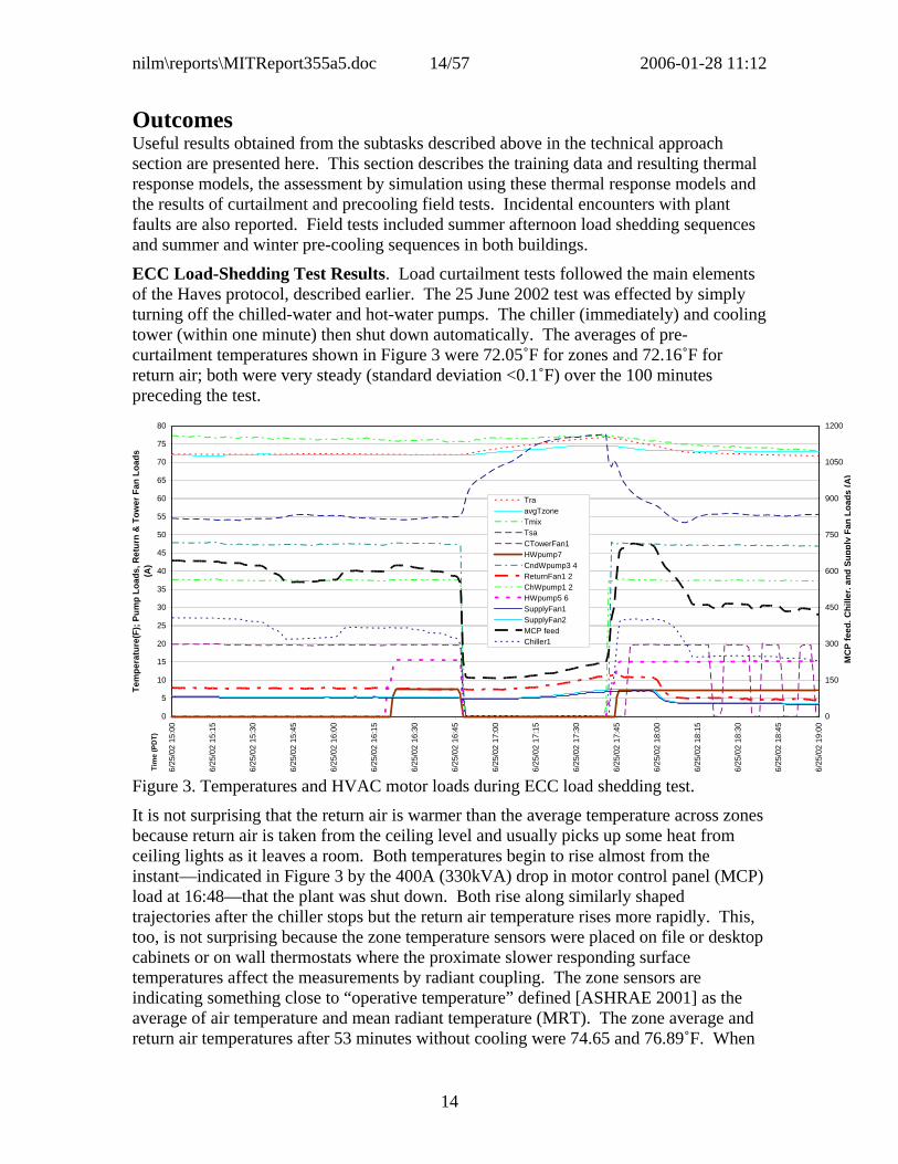
ECC Load-Shedding Test Results. Load curtailment tests followed the main elements of the Haves protocol, described earlier. The 25 June 2002 test was effected by simply turning off the chilled-water and hot-water pumps. The chiller (immediately) and cooling tower (within one minute) then shut down automatically. The averages of pre-curtailment temperatures shown in Figure 3 were 72.05˚F for zones and 72.16˚F for return air; both were very steady (standard deviation <0.1˚F) over the 100 minutes preceding the test.
0
5
10
15
20
25
30
35
40
45
50
55
60
65
70
75
80
6/25
/02
15:0
0
6/25
/02
15:1
5
6/25
/02
15:3
0
6/25
/02
15:4
5
6/25
/02
16:0
0
6/25
/02
16:1
5
6/25
/02
16:3
0
6/25
/02
16:4
5
6/25
/02
17:0
0
6/25
/02
17:1
5
6/25
/02
17:3
0
6/25
/02
17:4
5
6/25
/02
18:0
0
6/25
/02
18:1
5
6/25
/02
18:3
0
6/25
/02
18:4
5
6/25
/02
19:0
0
Tim
e (P
DT)
Tem
pera
ture
(F);
Pum
p Lo
ads,
Ret
urn
& T
ower
Fan
Loa
ds
(A)
0
150
300
450
600
750
900
1050
1200
MC
P fe
ed, C
hille
r, an
d Su
pply
Fan
Loa
ds (A
)
TraavgTzoneTmixTsaCTowerFan1 HWpump7 CndWpump3 4 ReturnFan1 2 ChWpump1 2 HWpump5 6 SupplyFan1 SupplyFan2 MCP feed Chiller1
Figure 3. Temperatures and HVAC motor loads during ECC load shedding test.
It is not surprising that the return air is warmer than the average temperature across zones because return air is taken from the ceiling level and usually picks up some heat from ceiling lights as it leaves a room. Both temperatures begin to rise almost from the instant—indicated in Figure 3 by the 400A (330kVA) drop in motor control panel (MCP) load at 16:48—that the plant was shut down. Both rise along similarly shaped trajectories after the chiller stops but the return air temperature rises more rapidly. This, too, is not surprising because the zone temperature sensors were placed on file or desktop cabinets or on wall thermostats where the proximate slower responding surface temperatures affect the measurements by radiant coupling. The zone sensors are indicating something close to “operative temperature” defined [ASHRAE 2001] as the average of air temperature and mean radiant temperature (MRT). The zone average and return air temperatures after 53 minutes without cooling were 74.65 and 76.89˚F. When
nilm\reports\MITReport355a5.doc 15/57 2006-01-28 11:12
15
the chiller is turned back on, the return air temperature again responds more quickly than the zone sensors and we see that it approaches within 0.1˚F of the pre-test temperature 50 minutes later. At this point the return temperature is 0.8˚F below the sluggishly responding average zone temperature. The return air temperature drops below the pre-test value (overshoots in the direction of initial response) after the chiller is restarted--a direct result of slow zone thermostat response. Fan power rises gradually during curtailment as air flow increases to satisfy terminal units demand for more cooling and static pressure is maintained. The pressure setpoint could be reduced to prevent this.
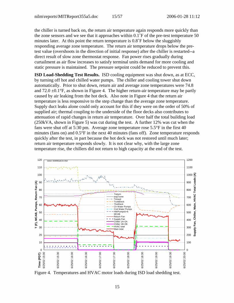
ISD Load-Shedding Test Results. ISD cooling equipment was shut down, as at ECC, by turning off hot and chilled water pumps. The chiller and cooling tower shut down automatically. Prior to shut down, return air and average zone temperatures were 74.8 and 72.0 ±0.1°F, as shown in Figure 4. The higher return-air temperature may be partly caused by air leaking from the hot deck. Also note in Figure 4 that the return air temperature is less responsive to the step change than the average zone temperature. Supply duct leaks alone could only account for this if they were on the order of 50% of supplied air; thermal coupling to the underside of the floor decks also contributes to attenuation of rapid changes in return air temperature. Over half the total building load (250kVA, shown in Figure 5) was cut during the test. A further 12% was cut when the fans were shut off at 5:30 pm. Average zone temperature rose 5.5°F in the first 40 minutes (fans on) and 0.5°F in the next 40 minutes (fans off). Zone temperature responds quickly after the test, in part because the hot deck was not restored until much later; return air temperature responds slowly. It is not clear why, with the large zone temperature rise, the chillers did not return to high capacity at the end of the test.
networ~1\t10035cat3.xls shed
0
10
20
30
40
50
60
70
80
90
100
110
120
6/25
/02
15:0
0
6/25
/02
15:3
0
6/25
/02
16:0
0
6/25
/02
16:3
0
6/25
/02
17:0
0
6/25
/02
17:3
0
6/25
/02
18:0
0
6/25
/02
18:3
0
6/25
/02
19:0
0
6/25
/02
19:3
0
6/25
/02
20:0
0
Tim
e (P
DT)
T (F
), M
CA
B, P
umps
, Ret
urn
Fan
(A)
0
100
200
300
400
500
600
700
800
900
1000
1100
1200
Supp
ly F
an, C
hille
r, M
ain,
HVA
C T
otal
Loa
ds (A
) Treturn avgTzoneTmixed TcoldDeck ThotDeck Ch Water Pumps Cnd Water Pumps HWPumps5+6 MCAB Return Fan Supply Fan Chiller 1A+2A Chiller 1B+2B HVAC total Main total
Figure 4. Temperatures and HVAC motor loads during ISD load shedding test.

nilm\reports\MITReport355a5.doc 16/57 2006-01-28 11:12
16
Zone Conditions for ECC. Zone temperatures (transient behavior and dispersion among zones) observed during the June 2002 site visit were analyzed to assess the consistency of zone thermal conditions. The zone temperatures, their average, and the standard deviation across zones, are plotted in Figures 5 and 6. Note that loggers resided together in a bag prior to deployment (2002.06.21 15:00-16:30 PDT), thus the data taken prior to deployment is only useful for showing that the loggers track each other quite well.
Figure 5. Children’s Court micro-logger data from launch time (2002.06.19 13:00 PDT) through first download/relaunch (2002.06.26 16:00-16:45 PDT).
Figure 6. Children’s Court zones before, during, after the chiller OFF step test of 25 June
Childen's Court/LA County: hobo-cct.xls
58
60
62
64
66
68
70
72
74
76
78
80
82
84
86
6/19
/02
12:0
0
6/20
/02
0:00
6/20
/02
12:0
0
6/21
/02
0:00
6/21
/02
12:0
0
6/22
/02
0:00
6/22
/02
12:0
0
6/23
/02
0:00
6/23
/02
12:0
0
6/24
/02
0:00
6/24
/02
12:0
0
6/25
/02
0:00
6/25
/02
12:0
0
6/26
/02
0:00
6/26
/02
12:0
0
Time (PDT)
T (F
)
0
2
4
6
8
10
12
14
16
18
20
22
24
26
28
Stan
dard
Dev
iatio
n A
cros
s Lo
gger
s (F
)
.
332630 332631332633 495199495205 522637522638 522640522641 522643522645 522646avg stDev
20020625 Childen's Court/LA County: hobo-cct.xls
64
66
68
70
72
74
76
78
80
12:0
0
12:3
0
13:0
0
13:3
0
14:0
0
14:3
0
15:0
0
15:3
0
16:0
0
16:3
0
17:0
0
17:3
0
18:0
0
18:3
0
19:0
0
19:3
0
20:0
0
20:3
0
21:0
0
21:3
0
22:0
0
22:3
0
23:0
0
23:3
0
0:00
0:30
1:00
1:30
2:00
2:30
3:00
Time (hh:mm PDT)
T (F
)
0
2
4
6
8
10
12
14
16
Stan
dard
Dev
iatio
n A
cros
s Lo
gger
s (F
)
.
332630 332631332633 495199495205 522637522638 522640522641 522643522645 522646avg stDev

nilm\reports\MITReport355a5.doc 17/57 2006-01-28 11:12
17
Children’s Court Precooling. A second ECC precooling test was completed 23 January 2003 in a week of mixed weather and building occupancy. Monday, 20 January, was sunny, Tuesday hazy, Wednesday and Thursday moderately overcast. Temperatures were typical for January except Wednesday morning was about 5°F below normal. The building was closed to the public on Monday for Martin Luther King Day. The chiller was turned off 17:00 PST on Wednesday afternoon and the supply fan static pressure (SP) setpoint was reduced from 2.2 to 0.5 inches (water gauge) at 01:00 early Thursday morning. The setpoint was restored to 2.2 inches at 07:00 and the chiller was restored at 10:15. The HVAC and building electrical loads are shown in Figure 7 and the temperature trajectories are plotted in Figure 8. The reason for large supply fan loads from 10:00 to noon Monday and Wednesday is unknown; some possibilities are a change in zone setpoints, a SP sensor fault, or some unexplained meddling with SP setpoint schedule. Note that the mean supply air temperature doesn’t change significantly even though its fluctuations are greatly diminished. Chiller power increases to maintain supply air temperature with the increased supply air flow rate. Chiller pump loads (not shown) are steady. Zone temperatures drop as would be expected in response to a step change in cooling capacity. Also note that the supply air temperature control loop is poorly tuned for part-load operation. The result is oscillation of the coil control valve, reflected in chiller power, at about 2.2 cycles per hour. The amplitude of these oscillations decreases during times of high cooling load (high supply air flow rate). The daily mean conditions, loads, and room temperatures averaged across 12 zones are summarized in Table 3. Because the chiller operates inefficiently at part load, there is little variation in average chiller power except on the day of the precooling test, when it was completely shut off
ml\work\10034\10034janx.xls main,chlr
0
200
400
600
800
1000
1200
0:00 6:00 12:00 18:00 0:00 6:00 12:00 18:00 0:00 6:00 12:00 18:00 0:00 6:00 12:00 18:00
Time (from 2003.01.20 00:00 PST)
P(kW
)
MainMCPsumChiller1SupplyFan2SupplyFan1
Figure 7. ECC electrical loads for 20-23 January 2003.

nilm\reports\MITReport355a5.doc 18/57 2006-01-28 11:12
18
ml\work\10034\10034janx.xls T
0
10
20
30
40
50
60
70
80
0:00 6:00 12:00 18:00 0:00 6:00 12:00 18:00 0:00 6:00 12:00 18:00 0:00 6:00 12:00 18:00 0:00
Time (from 2003.01.20 00:00 PST)
T (F
)
0
2
4
6
8
1
12
14
16
Tra Tmixed
Tsa OAT
Tz boilers
dPsaFan dPraFan
Figures 8. ECC temperatures; fan inlet velocity pressure and boiler duty cycle signals. Table 3. 24-Hour average conditions at Children’s Court for 20-23 January 2003 Monday Tuesday Wednesday Thursday CtowerFan (CT1) kW 1.8 1.3 1.3 1.5 CndWpump (P3) kW 28.2 28.3 25.6 10.3 ReturnFan (R1,R2) kW 0.3 0.3 0.3 5.3 SupplyFans (S1,S2) kW 100.4 90.6 81.5 74.9 HWpumps (P5,P6) kW 3.8 3.8 3.5 1.9 ChWpump (P1) kW 23.6 23.7 22.0 9.1 Chiller1 kW 236.7 222.1 203.5 99.6 MCP feed kW 394.8 370.0 337.6 202.7 C-H main kW 415.2 465.7 462.4 306.5 Tra °F 67.5 67.3 68.6 69.2 Tmixed °F 65.2 63.8 64.6 63.9 Tsa °F 55.8 55.8 56.6 59.7 Rhra % 49.9 52.8 51.6 50.3 Rhmixed % 44.8 51.4 45.0 40.8 Rhsa % 70.8 74.3 73.2 65.2 Tz (Hobos) °F 71.0 71.4 71.5 71.7 Tamb (outside) °F 60.1 58.5 57.2 61.9 S (plain LiCor) W/m2 154.1 114.2 75.9 77.1 Total (unshaded) W/m2 154.1 114.4 75.9 77.7 Diffuse1 (shaded) W/m2 27.7 55.9 55.3 62.3 Prt'l (partly shaded) W/m2 136.1 101.8 69.8 73.1
for 16 hours. The chiller average power Thursday was thus reduced from over 200 kW to 100 kW. The associated average cooling tower and chilled water pump loads were also reduced substantially from 49 to 21 kW. Supply fan power is about 16kW (4 kW daily

nilm\reports\MITReport355a5.doc 19/57 2006-01-28 11:12
19
average) during the precooling phase and about 112 kW during the day. Baseline chiller and pump power are very high Monday through Wednesday because no unoccupied periods were scheduled on the control system. The baseline daily average would have been about 150 kW for the chiller and 30 kW for pumps under a normal night lockout schedule. Estimated savings from this reduced baseline are, nonetheless, a considerable 45% which represents about $50k/year. The extra fan energy (compared to a fan-off-at-night baseline) is only about 10% of chiller and pump savings thanks to the reduced static pressure during precooling.
ISD Building Precooling. The test was completed Wednesday, 22 January. In contrast to Children’s Court, the ISD Building was partly occupied on the preceding Monday, 20 January 2003. Temperature trajectories are plotted in Figure 9 and HVAC and building electrical loads are plotted in Figure 10.
For this precooling test the chiller was turned off 18:00 PST on Tuesday afternoon and restored at 13:50 the following day. The windows were opened at 21:30 Tuesday and the return fan was started. Return temperature dropped from 73.2 to 69.0°F and average room temperature dropped from 73.5 to 64.3 F during the precooling period, which ended at 05:30 Wednesday morning with closing of the windows. The supply fan started at 05:40 per its normal schedule. The exhaust damper was closed and the return damper opened from 07:00 to 8:45 allowing the occupied space temperature to rise from 67.9 to 71.7°F. The space was thus effectively in a tempering mode from 05:30 to 08:45. This amount of tempering is more than was necessary; tempering would have ended at 07:20 when the zone reached 70°F, had the controls been properly automated.
Average zone temperature reached 74°F at 11:45am. The chiller remained locked out until13:50, by which time the zone temperature had reached 75.1°F. The return fan remained on through 24 January but the windows were not opened that night. This resulted in limited precooling Thursday morning by outside air being drawn through the hot and cold deck systems even though the supply fan was off. Note that return
ml\work\10035\10035dec.xls ncJa22f
0
20
40
60
80
100
120
0:00 8:00 16:00 0:00 8:00 16:00 0:00 8:00 16:00 0:00 8:00 16:00 0:00 8:00 16:00 0:00 8:00
Time (from 2003.01.19 0:00 PST)
T(F)
; Fan
s an
d C
hille
rs (k
W)
0
40
80
120
160
200
240
mai
n(kW
)
Tra OATThot TcoldavgTz SfanCh1B2B Ch1A2ARfan main
Figure 9. ISD temperatures and electric loads during week of the precooling test.

nilm\reports\MITReport355a5.doc 20/57 2006-01-28 11:12
20
temperature approaches room temperature progressively more closely from Monday (after the previous week and weekend in which there was no precooling) to Thursday. Several days of precooling are needed to cool the building’s floor deck structures from their under (ceiling plenum) sides. It is fair to conclude that 1) a one-day test is not sufficient to demonstrate the full potential and 2) precooling on Saturday, as well as Sunday, night may be cost effective. Chiller cycling is apparent in Figure 9. Details of this cyclic behavior are shown to better advantage on the expanded time scale of Figure 10. One may conclude that the cycling could be largely eliminated by modifying the compressor sequencing logic so that compressors come on one by one, rather than in pairs. The response to precooling is presented on an expanded time scale in Figure 11 where the cycling tendency, even under the heavy zone temperature pull-down load that existed when the chillers were finally started at ~14:00, can be clearly seen. The daily mean conditions, loads, and room temperatures averaged across six zones are summarized in Table 4. The ISD chillers, in contrast to the Children’s Court chiller, operate more efficiently at part load (in spite of the cycling). The average chiller input is therefore significantly lower on cooler and partial occupancy days. Average chiller power on the day of the precooling test is, nevertheless, less than half of the average power used on the other three days. Fan power, on the other hand, changes little from day to day except that average return fan power is higher Tuesday through Thursday because it was run during certain unoccupied hours on all three of those days. On the day of precooling, average chiller power was reduced from ~22 to 8.3 kW. Associated average cooling tower and chilled water pump loads also dropped substantially from ~8 to 3.7 kW. Average return fan power increases from ~7 to almost 13 kW. Net average savings are therefore about 12 kW from a baseline of 58 kW representing about $15,000/year. Precooling by supply fan would reduce savings by roughly half these amounts.
networ~1\20030121\t10035-01222003-011356.xls
0
10
20
30
40
50
60
70
9:10 9:20 9:30 9:40 9:50 10:00 10:10 10:20 10:30 10:40 10:50 11:00 11:10 11:20 11:30 11:40 11:50 12:00 12:10 12:20 12:30 12:40 12:50 13:00 13:10
Time (2003.01.21 PST)
(kW
/ph)
0
20
40
60
80
100
120
140
mai
n
(kW
/ph)
Sfan Ch1B2BChWP CndWPCh1A2A RfanHWP CThvac main
Figure 10. Short segment of Figure 9 showing compressor cycles (1m-average loads)

nilm\reports\MITReport355a5.doc 21/57 2006-01-28 11:12
21
nl\work\10035\10035dec.xls ncjA22X2
0
20
40
60
80
100
120
18:00 21:00 0:00 3:00 6:00 9:00 12:00 15:00 18:00Time (from 2003.01.21 18:00 PST)
T(F)
; Fan
s an
d C
hille
rs (k
W)
0
40
80
120
160
200
240
mai
n(kW
)
Tra OATThot TcoldavgTz SfanCh1B2B Ch1A2ARfan main
Figure 11. One-day segment of Figure 9 showing precooling test details. Table 4. Daily Summary ISD Building Data for 20-23 January 2003
Monday Tuesday Wednesday Thursday Chiller1 kW 12.45 13.88 5.58 9.87 Chiller2 kW 8.97 10.18 2.74 6.32 ChWpumps kW 2.57 2.98 1.16 2.37 CtowerFans kW 4.45 5.16 1.99 4.10 CndWpumps kW 1.15 1.14 0.54 0.81 ReturnFan kW 6.94 8.56 12.80 9.96 SupplyFans kW 18.19 18.27 18.19 17.93 Hwpump kW 0.89 0.89 0.87 0.88 HVAC feed kW 58.14 63.94 46.02 54.75 ISD main kW 111.61 173.73 157.20 163.46 Tra F 67.3 69.6 72.0 69.8 Rhra % 54.7 52.2 49.1 49.7 Thot °F 84.0 84.5 79.1 76.3 Tcold °F 60.2 59.6 61.8 59.9 Rhcold % 60.5 63.7 61.5 60.3 Rhmix % 37.5 41.4 53.8 53.3 B1lo s/min 21.1 19.6 13.8 0.0 B2lo s/min 35.3 34.9 33.7 35.3 B2hi s/min 5.5 4.6 18.6 27.4 Tz (Hobos) °F 71.6 72.0 70.8 72.2 Tamb (outside) °F 59.4 58.5 57.2 61.9 S (plain LiCor) W/m2 154.1 114.3 76.0 77.1 Total (unshaded) W/m2 154.1 114.4 75.9 77.7 Diffuse1 (shaded) W/m2 27.7 55.9 55.3 62.3 Prt'l (partly shaded) W/m2 136.1 101.8 69.8 73.1 Barometer PSIA 14.59 14.61 14.64 14.59

nilm\reports\MITReport355a5.doc 22/57 2006-01-28 11:12
22
Model Identification. The discrete-time, linear (CRTF) model developed in the technical approach section will be used to simulate the dynamic thermal responses of the two test buildings. The parameters for each model must therefore be determined by least-squares fit to the monitored conditions and thermal responses of each building. Sol-air temperature and time-shifted zone temperature are converted to temperature differences by subtracting current zone temperature from the other (current and lagged) temperatures. This eliminates the current zone temperature term and reduces the order of the least squares problem by one, and results in a solution that satisfies the constraint on sums of temperature coefficients. The model identified for ISD is in the form of (8) with one thermal capacitance and hour time steps: )8(),(),(),( 0010, zz
nww
nzz
nzz TBTBQBQ θθφφ −+=−
With φz,0 equal minus one, the least squares solution is Qz,k = Qz,k–1 + 194.4Tz,k – 198.1Tz,k–1 + 0.2249Tx,k + 3.456Tx,k–1 where T is in °F and Q is in kW. The building load coefficient (UA) corresponding to these estimated model coefficients is 16367 Btuh/°F. The normalized width of each coefficient’s confidence interval (CI) is given in Table 5. Table 5. ISD model confidence intervals
Term Coefficient CI/|coef| Q,k–1 0.7751 212.5 Tx,k–0 -0.2249 0.745 Tx,k–1 -3.456 11.3 Tz,k–0 194.4 109.3 Tz,k–1 -198.1 109.3
The response produced by the model for ISD is compared to the measured response in Figure 12.

nilm\reports\MITReport355a5.doc 23/57 2006-01-28 11:12
23
Figure 12. Measured and simulated trajectories of ISD net zone heat gain from HVAC air streams, solar radiation and electrical loads.
The model identified for the ECC is in the form of (7) with two thermal capacitances and hour time steps: ),(),(),( 1000, zz
nww
nzz
nzz TBTBQBT θθφθ −+=
With θz,0 equal one, the least squares solution is Tz,k = .8873Tz,k–1 + .0991Tz,k–2 + .2580Tx,k – .0323Tx,k–1 + .0201Tx,k–2 + .00160Q where T is in °F and Q is in kW. The building load coefficient (UA) corresponding to these estimated model coefficients is 29004 Btuh/°F. This is about twice the UA of ISD, which is reasonable for a much larger, albeit better insulated, building. The normalized width of each coefficient’s confidence interval (CI) is given in Table 6. Table 6. ECC model confidence intervals Term Coefficient CI/|coef| Tz,k–1 0.8873 10.8 Tz,k–2 0.0991 1.2 Tx,k–1 -0.0323 1.0 Tx,k–2 0.0201 1.0 Q 0.0160 3.4
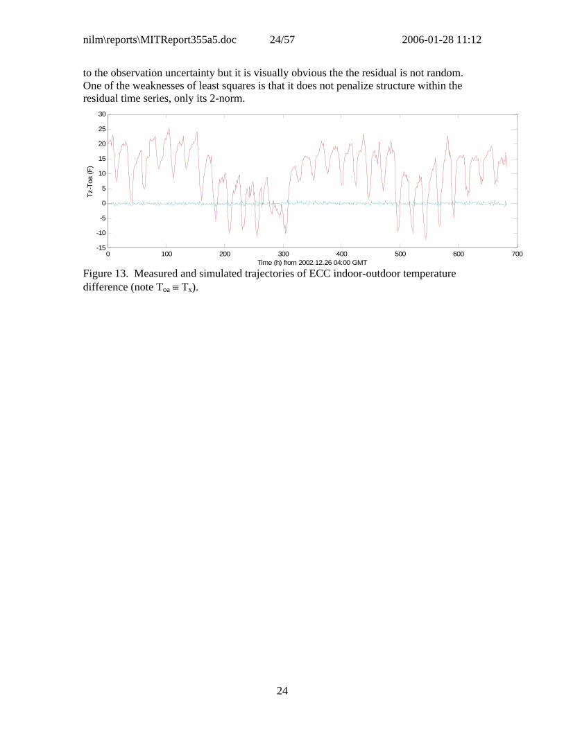
The response produced by the model for ECC is compared to the measured response in Figure 13. The magnitude of the root-mean-square of the residual, 0.33°F, is comparable
0 48 96 144 192 240 288 336 384 432 480-800
-600
-400
-200
0
200
400
600
800
1000
Time (hr from 20020907 07:00 GMT)
Net Direct Aggregate Zone Heat Gain (kBtuh)Blue - MeasuredRed - Simulated
nilm\reports\MITReport355a5.doc 24/57 2006-01-28 11:12
24
to the observation uncertainty but it is visually obvious the the residual is not random. One of the weaknesses of least squares is that it does not penalize structure within the residual time series, only its 2-norm.
0 100 200 300 400 500 600 700-15
-10
-5
0
5
10
15
20
25
30
Tz-T
oa (F
)
Time (h) from 2002.12.26 04:00 GMT Figure 13. Measured and simulated trajectories of ECC indoor-outdoor temperature difference (note Toa ≡ Tx).

nilm\reports\MITReport355a5.doc 25/57 2006-01-28 11:12
25
Peak-Shifting Case Study Results. The night precooling control strategies have been evaluated by using TMY2 Los Angeles weather data to drive the ISD thermal response model. The cooling capacities provided by the chiller plant and by outside air are separately integrated over the year for each case simulated. These numbers and the annual electricity (energy and demand) costs together provide a complete picture of the alternative control strategies described in the Technical Approach section. The base case, no night cooling with the economizer setpoint equal to the mechanical cooling setpoint (74.5°F), is shown in Figure 14. Mechanical cooling represents almost 60% of the total annual load. As the economizer setpoint is reduced, the total cooling load is increased but the annual mechanical cooling share is reduced to about 50% of the total with the most extreme economizer setpoint of 68°F. The cooling shares are not very sensitive to economizer setpoint because there is little daytime economizer cooling potential on days when there would be significant chiller load without economizer cooling. With economizer cooling enabled at night (fan runs whenever zone temperature is above the economizer setpoint and outdoor temperature is below zone temperature) mechanical cooling is immediately reduced by 30% for case 6 (economizer setpoint = mechanical cooling setpoint = 74.5°F) simply by eliminating morning pull down loads. Total annual cooling is immediately increased by 20% in response to lower zone temperatures on many nights. Note, furthermore, that the mechanical share drops significantly (an additional 30%) and total load increases significantly (another 17%) as the economizer setpoint is lowered. These results are shown in Figure 15. Figure 14. No night cooling, cases 1-5.
work\tmy10035d.xls Donly
0
500
1000
1500
2000
2500
3000
3500
4000
74.5 74 72 70 68
Economizer Setpoint (F)
Ann
ual C
oolin
g (M
Btu
)
economizer mechanical

nilm\reports\MITReport355a5.doc 26/57 2006-01-28 11:12
26
Figure 15. All night cooling, cases 6-10. Figure 16. Delayed-start night cooling, cases 11-15.
work\tmy10035d.xls D&N
0
500
1000
1500
2000
2500
3000
3500
4000
74.5 74 72 70 68Economizer Setpoint (F)
Ann
ual C
oolin
g (M
Btu
)economizer mechanical
work\tmy10035d.xls D&N
0
500
1000
1500
2000
2500
3000
3500
4000
74.5 74 72 70 68Economizer Setpoint (F)
Ann
ual C
oolin
g (M
Btu
)
economizer mechanical

nilm\reports\MITReport355a5.doc 27/57 2006-01-28 11:12
27
With optimal nightly delayed-start times, the annual fan energy (hours of fan operation) is greatly reduced, the amount of economizer cooling is moderately reduced, and the amount of mechanical cooling is increased slightly as shown in Figure 16. Total annual cooling numbers are 10-15% lower. However, as shown in Figure 17, there is very little cost savings because off-peak energy rates are relatively low.
0
20000
40000
60000
80000
100000
120000
140000
160000
180000
200000
1 2 3 4 5 6 7 8 9 10 11 12 13 14 15
Case#
Ann
ual E
lect
ricity
Cos
t ($)
RatchetOn-Peak kWMid-Peak kWOff-Peak kWOn-Peak kWhMid-Peak kWhOff-Peak kWh
Figure 17. Annual electricity costs (building total) by time of use, energy, and demand.

nilm\reports\MITReport355a5.doc 28/57 2006-01-28 11:12
28
Conclusions and Recommendations Thermal and Electric Load Response Models. Real-time estimation of the near-term curtailment resource and control of night precooling both require models of transient envelope thermal response and static plant part-load efficiency [Gordon and Ng, 2000]. The envelope model and identification procedure developed for this project requires several weeks of hourly data for weather (sunshine, temperature, wind), internal gains (lights and plugs), and HVAC (sensible heating and cooling; return air temperature).
By forcing the identified model to satisfy applicable thermodynamic constraints, the need for a priori information about the thermal envelope and capacitance of contents and structure is eliminated. This is an important step towards completely autonomous model identification that must be achieved for such model-based control to be successfully commercialized. Second order linear models were sufficient to predict sensible loads and conditioned-space temperatures within the confidence interval of the training data.
Curtailment. Using an aggressive interpretation of the Haves protocol, the afternoon load shedding tests reduced whole building load by up to 60% (1.2 W/ft2 for ECC and 3.6 W/ft2 for ISD) and HVAC loads by essentially 100%. Leaving chillers off for one hour resulted in zone temperatures increasing by 2.6 ˚F for ECC and 5.5˚F for ISD and return air temperatures increasing by 4.7 ˚F for ECC and 2.7˚F for ISD.
Chiller part-load efficiency is a significant factor in curtailment strategy. With good part-load efficiency a partial reduction of cooling capacity results in significant load reduction but sufficient remaining cooling capacity to extend the duration of a typical curtailment from less than one hour to at least two, and perhaps four hours as required for a single building to qualify for curtailment incentives. If part-load efficiency is such that the chiller must be completely shut down to obtain program-imposed load reduction, the duration will most likely not be sufficient to qualify for incentives. It is this common situation, in part, that has sparked interest of control of buildings in aggregates. Some of the questions this research cannot answer include 1) who can best (in a cost/benefit sense) coordinate building-level load curtailment, and 2) what incentives suffice to engage building owners in load curtailment actions? LA County was initially interested in the program [http://www.pge.com/002_biz_svc/loadmgmt_programs.shtml] that called for curtailment in 100kW, 4-hour blocks. However, after some experience with the costs and benefits, the county has decided not to participate.
The model and identification method developed in this project allow a building operator to forecast the load shedding potential (load delta and duration) at a given time. The utility knows its capacity limits, can forecast system wide loads and can thus estimate quite well on any given morning the curtailment trajectory required that afternoon. The curtailment coordinator ideally has both sets of information, as well as the ability to control (directly or via a commitments from building owners) a set of buildings that, in aggregate, represent a sufficient demand responsive resource. Moreover, uncertainties in the forecasts and effectiveness of control require safety margins. The foregoing arrange-ments represent significant transaction costs for communication and contractual infrastructure.

nilm\reports\MITReport355a5.doc 29/57 2006-01-28 11:12
29
There is also significant cost and uncertainty in measurement and verification. Simple models for allocating incentives are attractive because they appear to involve smaller transaction costs. However, simple models are not adequate for control. Since control is key to the entire program the utility or aggregator might as well use the model that is required for control to more accurately allocate incentives as well. At least the transaction cost of maintaining more than one model is eliminated.
Night Precooling. Night precooling was shown to reduce annual mechanical cooling energy input by up to 50%. Control of night precooling involves the same building-specific thermal response model that is used for curtailment.
Because it is primarily a controls measure, the implementation cost for night cooling is potentially quite low. However, there are some situations where significant modification to air distribution and control systems will be needed. To prevent the initially coolest zones from getting too cold, it is important that terminal boxes be capable of closing fully. This has not traditionally been a design criterion because, in occupied period operation, there is a minimum air setting based on ventilation needs. The ability of the control system to execute the optimization algorithm (Appendix G) is a key issue. Finally, it is necessary that the control system support global zone setpoint changes, either by storing multiple arrays of set points, e.g. “daytime,” “night precooling,” and “night no cooling,” with a schedule determining which array is in effect at a given time, or by allowing a single command to shift all setpoints up or down by a specified amount.
There are significant implementation barriers involving energy and associated cost of fan operation and limitations imposed by existing control systems. For buildings with constant volume fan systems, the potential savings for night cooling are an added incentive to convert to VAV. However, fan energy costs are significant even in VAV systems. A scheme to reduce pressure drop and provide additional control over which parts (underside or top of floor deck) of the structure are cooled is presented in Appendix H.
Fault Detection. A number of faults were identified from the data by inspection. The Children’s Court has large temperature variations across zones. The cooling tower fan cycles excessively. One return fan is down and control of building pressure, minimum outside air and economizer cooling suffer as a result. The coordination of building fans, cooling tower fans and the chiller appears to be significantly sub-optimal. Except for the interzonal temperature variations, all of this can be inferred by inspection (potentially automatable) of NILM data.
The ISD has serious control faults involving the modulation of chiller and cooling tower capacity. At one point the chiller capacity increased from stage 1 to stage 4 abruptly (<100s). The cooling tower staging setpoints are also incorrect resulting in considerable tower fan cycling. These faults are detectable from NILM data alone.
Other ISD faults require analysis of thermal time-series data that are, in general, already monitored in most CV dual deck systems by their existing HVAC controls. Coordination of hot deck temperature and damper position is poor, with the result that simultaneous heating and cooling increases with cooling load. Both dampers (or at least the hot deck damper) should be shut when the fans are off. One of the two boilers should be shut down completely in summer. Control of hot deck temperature is difficult in part because

nilm\reports\MITReport355a5.doc 30/57 2006-01-28 11:12
30
the boiler setpoint temperature is fixed. Some means should be found to prevent the boiler-coil convection loop that develops when pumps and fans are off. Hot- (and possibly cold-) deck duct leakage appear to be excessive.
The discovery of HVAC and controls faults is not surprising in light of our experiences in other buildings. Faults that do not result in persistent occupant complaints often go undetected or, if detected, un-repaired. To have found such a large number of faults within the first few days’ of monitored data is, however, quite remarkable.
Additional faults have been identified by visual observation. Both ECC and ISD buildings have been operated with supply air duct access doors and pressure relief doors open or exhibiting large leaks. The ISD condensate pan leaks so badly that most of the condensate puddles on the mixed air plenum floor rather than being channeled directly to the building waste-water line. Economizer controls in both buildings suffer from excessively conservative set points and unnecessarily low outdoor air lockout temperatures. References ASHRAE. 2001. Handbook of Fundamentals, Atlanta Armstrong, P.R. and P.D. Heerman. 1985. "uP-based hot-wire anemometry," First National Conference on Microcomputer Applications for Conservation and Renewable Energy, Tucson, AZ. Braun, J.E. and Nitin Chaturvedi, 2002. “An inverse grey-box model for transient building load prediction,” Int’l J. HVAC&R Research, 8(1) pp.73-99. Gordon, J.M, and K.C. Ng, 2000. Cool Thermodynamics, Cambridge International Science Publishing ISBN 1898326 908. Haves, P., and F. Smothers, 2002. Guidelines For Emergency Energy Reduction In Commercial Office Buildings (LBNL Report) Hittle, D.C. and R. Bishop, 1983. “An improved root-finding procedure for use in calculating transient heat flow through multilayered slabs,” Int’l J Heat Mass Transfer, 26(11) 1685-1693. Luo, Dong. 2001. Detection and Diagnosis of Faults and Energy Monitoring of HVAC Systems with Least-Intrusive Power Analysis. MIT PhD Thesis. Seem, J.E., 1987. Heat Transfer in Buildings, PhD Thesis, UW, Madison. Seem, J E. and J.E. Braun, 1991. Adaptive methods for real-time forecasting of building electrical demand, ASHRAE Trans. 1991, vol.97, Part 1, paper# NY-910-10-3, 710-721. http://www.pge.com/002_biz_svc/loadmgmt_programs.shtml (PG&E) http://www.caiso.com/SystemStatus.html (ISO capacity, load forecast, stage notice)

nilm\reports\MITReport355a5.doc 31/57 2006-01-28 11:12
31
Appendix A. ISD Building Description
The ISD Building is a 70,000 ft2 structure built in 1973 with a constant volume dual duct HVAC system. The plant consists of two boilers and two four-stage reciprocating chillers. Two NILMs have been installed, one at the service entrance and one at the central fan/chiller motor control panel. Thermal instrumentation includes temperature and humidity of return-, mixed-, hot-deck and cold-deck air. Fan inlet pressure taps measure flow rates at the supply and return fans while thermal anemometers measure “mass velocity” (labeled “rhoV” in the plots) to determine the damper-controlled division of supply air between hot- and cold-decks. Table A-1. ISD Building HVAC Electrical Loads.
Circuit & Motor Ratings Name Function Ckt Amps HP rpm P1 Chilled water pump 1 30 7.5 P2 Chilled water pump 2 30 7.5 P3 Condenser water pump 1 30 10 P4 Condenser water pump 2 30 10 P5 Hot water pump 1 15 1.5 P6 Hot water pump 2 15 1.5 CP1 Circulation pump 1 0.5 SF Supply fan 200 60 RF Return fan 60 20 C1.1 Chiller stage 1 compressors C1.2 Chiller stage 2 compressors C1.3 Chiller stage 3 compressors C1.4 Chiller stage 4 compressors 300 TF1A Toilet fan 1A TF1B Toilet fan 1B TF2 Toilet fan 2 EF1 Exhaust fan 1 0.5 EF2 Exhaust fan 2 0.5 EF3 Exhaust fan 3 EF4 Exhaust fan 4 0.33 EF5 Exhaust fan 5 0.25 EF6 Exhaust fan 6 0.75 CAC1 Control air compressor 1 1 CAC2 Control air compressor 2 1 Strip heater, 13kW Internal Services Department (ISD) Building BIS#7022; LACO#5863 Completion date: 1 May 1973 1100 N Eastern Avenue Lighting retrofit: 29 November 1996 Los Angeles, CA 90063 Floor area net/gross (ft2): 58,826/45,646 Function: Offices Operating hours: 11 (Monday-Thursday) Heat: two 1.1 Mbtuh (input) gas-fired hot water boilers Cooling: two 2-stage reciprocating chillers Distribution: Dual-duct constant volume system; built-up AHU Electric Utility: SCE, I-6 (interruptible) rate

nilm\reports\MITReport355a5.doc 32/57 2006-01-28 11:12
32
Contact: Ron Mohr Table A-2. ISD Building K20 Channel Assignments (all are A-phase currents).
Circuit & Motor Ratings K20 Channel Name Function Ckt Amps HP
CT FS amps
2 P1 Chilled water pump 1 30 7.5 25 2 P2 Chilled water pump 2 30 7.5 3 P3 Condenser water pump 1 30 10 50 3 P4 Condenser water pump 2 30 10 7 P5 Hot water pump 1 15 1.5 10 7 P6 Hot water pump 2 15 1.5 6 CP1 Circulation pump 1 0.5
0 SF Supply fan 200 60 150 5 RF Return fan 60 20 50
1 C1B+2B Chiller stages 3&4 (both chillers) 300 4 C1A+2A Chiller stages 1&2 (both chillers) 6 TF1A Toilet fan 1A 10 6 TF1B Toilet fan 1B 6 TF2 Toilet fan 2 6 EF1 Exhaust fan 1 0.5 6 EF2 Exhaust fan 2 0.5 6 EF3 Exhaust fan 3 6 EF4 Exhaust fan 4 0.33 6 EF5 Exhaust fan 5 0.25 6 EF6 Exhaust fan 6 0.75 6 CAC1 Control air compressor 1 1 6 CAC2 Control air compressor 2 1 6 Strip heater, 13kW 8 LAC G,1,2 floor lighting (w/retrofit) 150 9 DSA General plug loads 300 10 MCAB Penthouse HVAC loads (CT) 100 11 Lift1+2 Hydraulic elevators 150 12 DEA Emergency loads 150 13 LAG 3rd floor lighting (no retrofit) 50 14 Main Service entrance (5A piggy back CT) 1500 15 MCA Main HVAC loads 600

nilm\reports\MITReport355a5.doc 33/57 2006-01-28 11:12
33
NILM Load Data. HVAC loads were cycled on and off, one load at a time, while recording at 120Hz the power, P, and reactive power, Q, fed to the MCC. Second and higher harmonic spectral envelopes were not recorded during these training tests. When interpreting the recorded signals it is important to keep in mind that the spectral envelope is not an instantaneous signal but rather a one-cycle moving average of the selected harmonic (in this case the 60Hz fundamental) of the power signal. Each pump was turned on, allowed to run for about 10 seconds, turned off, and left off for about 10 seconds. This standard on/off sequence was repeated five times for each pump. The supply and return fans were operated longer because they have longer start transients. The chillers also produced long on cycles because they have a programmed multi-stage sequence control that requires operation at a given stage for a minimum time before switching to the next higher stage. V-sections were fit to all start and stop transients by the interactive Matlab program vtrain. The program locates events and allows the user to define the section boundaries and averaging weights used to aggregate points taken from all (or a subset) of the observed transients. The mean values of P and Q and their standard deviations, computed for data points recorded after each load had reached steady state, are presented in Table A-3. The steady state means and standard deviations serve two purposes. The real (P) and reactive (Q) components are used to identify off transitions and the real component is used to estimate energy used by a given load during each of its operating periods. Standard deviations are generally 1% of average load. However, the standard deviations for the two small pumps (P5 and P6) are about 3% of average load. These numbers suggest a simple "base-value-plus-percent-of-signal" noise model. Note that two sets of lead-lag pumps have significantly different steady state loads: P1,P2 (chilled water) and P5,P6 (heating water). Table A-3. Loads recorded during ISD NILM training (multiply P and Q values by 20).
Circuit & Motor Ratings P (W) Q (VAR) Change Name Function Ckt Amps HP Rpm Average s.d. Average s.d. PF P(W) Q(VAR) PF P1 ChW 30 7.5 287.7 2.9 -344.9 2.5 0.64 P2 ChW 30 7.5 268.1 2.7 -202.5 2.3 0.80 P3 CndW 30 10 488.7 4.3 -336.7 2.6 0.82 P4 CndW 30 10 465.3 5.0 -332.8 2.8 0.81
P5 HW 15 1.5 69.7 2.3 -87.3 2.2 0.62 P6 HW 15 1.5 77.8 2.1 -98.8 2.2 0.62
S+R Fans 1869 42 -1456 13 0.79 SF fan 200 60 1460 35 -1092 7 0.80 409 -364 0.75RF Fan 60 20 476 28 -391 10 0.77
Fans 2002 40 -1420 26 0.82
C1.1 Chiller 2775 45 -2115 26 0.80 773 -695 0.74C1.2 Chiller 4162 47 -3470 23 0.77 1387 -1354 0.72C1.3 Chiller 5581 55 -5023 22 0.74 1419 -1553 0.67C1.4 Chiller 300 6762 48 -6475 17 0.72 1181 -1453 0.63

nilm\reports\MITReport355a5.doc 34/57 2006-01-28 11:12
34
ISD Floor, Wall and Window Areas The ISD is built on a 24’x24’ structural grid 10 bays wide (the long side running almost east to west; the “south” wall normal actually points ~30 degrees east of south) and 4 bays deep (the short side). The main footprint is thus a bit over 240’x 96’= 23,000 ft2 . The basement is only 3 bays deep (floors 1 and 2 extend 1 bay further north) giving it a ~240’x 72’= 17,300 ft2 footprint. The basement is essentially windowless. Windows on the main floors (1 and 2) are placed every 4 feet to fit the 24-foot grid and the floor-to-floor height is 14 feet. The windows are operable (!) but usually remain closed. The third floor (penthouse) has no windows except on the 50-foot east wall, looking on to a rooftop terrace, which is essentially all glass with a 20” (clear) transom strip of fixed glazings above an 80” (clear) main span of sliding doors and fixed glazings.
There are roof doors at the tops of both stairwells, one at the north-east corner (north-most point) and one near the center of the west end of the building (just west of and adjacent to the elevators).
Window types are described in Table A-3 and their aggregate surface areas are summarized by location in Tables A-4 and A-5.
Table A-4. ISD Window Types
Dimensions (H x W, in.) Clear Mullion
Type Finished Clear Area (ft2) Area (ft2)
A (single casement) 66.0 x 36.5 61.5 x 31.25 13.35 3.38
B (narrow fixed) 108.0 x 17.0 64.7 x 13.5
36.0 x 13.5
9.44 3.31
C (wide fixed) 108.0 x 99.0 64.7 x 95.5
36.0 x 95.5
66.78 7.47
D (door) 83.5 x 36.0 66.7 x 24.8 11.35 9.53
E (narrow transom) 24.0 x 72.0 20.0 x 70.5 9.79 2.21
G (double casement) 66.0 x 22.5 61.5x18.3 7.82 2.50
I (sliding door) 83 x 36 80 x 33 18.33 2.42
J (door-height, fixed) 83 x 40 80 x 37 20.56 2.50
K (transom) 23 x 40 20 x 37 5.14 1.25
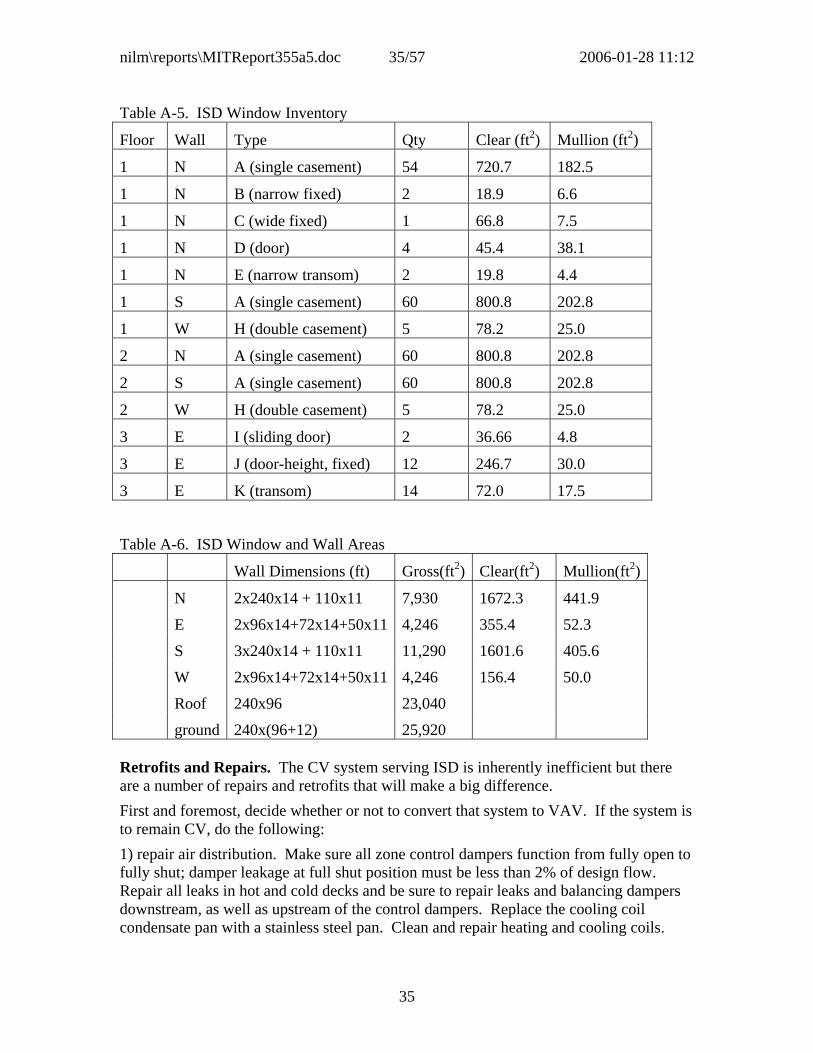
nilm\reports\MITReport355a5.doc 35/57 2006-01-28 11:12
35
Table A-5. ISD Window Inventory
Floor Wall Type Qty Clear (ft2) Mullion (ft2)
1 N A (single casement) 54 720.7 182.5
1 N B (narrow fixed) 2 18.9 6.6
1 N C (wide fixed) 1 66.8 7.5
1 N D (door) 4 45.4 38.1
1 N E (narrow transom) 2 19.8 4.4
1 S A (single casement) 60 800.8 202.8
1 W H (double casement) 5 78.2 25.0
2 N A (single casement) 60 800.8 202.8
2 S A (single casement) 60 800.8 202.8
2 W H (double casement) 5 78.2 25.0
3 E I (sliding door) 2 36.66 4.8
3 E J (door-height, fixed) 12 246.7 30.0
3 E K (transom) 14 72.0 17.5
Table A-6. ISD Window and Wall Areas
Wall Dimensions (ft) Gross(ft2) Clear(ft2) Mullion(ft2)
N 2x240x14 + 110x11 7,930 1672.3 441.9
E 2x96x14+72x14+50x11 4,246 355.4 52.3
S 3x240x14 + 110x11 11,290 1601.6 405.6
W 2x96x14+72x14+50x11 4,246 156.4 50.0
Roof 240x96 23,040
ground 240x(96+12) 25,920 Retrofits and Repairs. The CV system serving ISD is inherently inefficient but there are a number of repairs and retrofits that will make a big difference. First and foremost, decide whether or not to convert that system to VAV. If the system is to remain CV, do the following: 1) repair air distribution. Make sure all zone control dampers function from fully open to fully shut; damper leakage at full shut position must be less than 2% of design flow. Repair all leaks in hot and cold decks and be sure to repair leaks and balancing dampers downstream, as well as upstream of the control dampers. Replace the cooling coil condensate pan with a stainless steel pan. Clean and repair heating and cooling coils.

nilm\reports\MITReport355a5.doc 36/57 2006-01-28 11:12
36
2) Upgrade zone controls to DDC with e/p interface to existing damper actuators. All zone temperatures must be available to, and all actuator positions must be commandable by, the supervisor. All temperature sensor locations must provide reasonable estimate of average zone temperature (±°F) with fans on or off and not be adversely influenced by direct solar gains, zone supply air temperature, or heat generated by electric lights, computers, and other equipment. In particular, supervisor must be able to reset hot and cold deck temperatures such that simultaneous heating and cooling are minimized or, alternatively, total cost of central plant operation is minimized. 3) Upgrade central plant equipment. Install 2-speed chilled water pumps or replace with VSD pumps. Install 2-speed condenser water pumps or replace with VSD pumps. Install 2-speed cooling tower fans or replace with VSD fans. 4) Upgrade central plant controls. Replace zone temperature control loops so that setpoints can be centrally controlled and local loop temperature and damper positioning commands are available to the supervisory control system. Replace pneumatic hot and cold control loops with DDC. Replace boiler temperature controls with DDC so that boiler temperature can be reset. Replace chilled water temperature control loop with DDC so that it can be reset by the supervisor. Reprogram (or replace with appropriately programmable) compressor sequence controls so that supervisor can select local loop control on chilled water or cold deck temperature or over-ride for modes such as optimal start or curtailment; compressors should come on one at a time alternating between the north and south chiller units and commissioning should check that when one chiller is off line for service, the appropriate number of compressors come on in the other chiller. Install DDC local loop controls to make chilled water, condenser water, and tower air flow rates approximately proportional to chiller load when in fail-safe mode but program supervisor to control operation for maximum whole plant efficiency in normal operating mode. Cooling tower air and water-side discharge temperatures and cooling coil air- and water-side inlet and outlet temperatures must be available to the supervisor. 5) Adjust and upgrade economizer controls. Clean, repair and adjust dampers and existing pneumatic actuators. Replace existing pneumatic control loop with DDC including an accurate, properly shielded outdoor air temperature sensor (ok to be from another building on the N. Eastern Ave. campus) an accurate and properly situated mixed air sensor, and an accurate and properly situated return air temperature sensor. All signals and damper commands available to supervisor. 6) Rebalance air system to provide uniform supply air flow over conditioned floor area, correct building pressure, and correct ventilation air to each zone. If a VAV retrofit is pursued, replace recommendations (1), (2) and (6) with actions appropriate to the VAV system. In particular, the supervisor must still be able to reset hot and cold deck temperatures such that simultaneous heating and cooling are minimized or, alternatively, total cost of central plant operation is minimized. In addition, supply air static pressure reset control and demand ventilation control should be provided so that fan power can be controlled by the supervisor in conjunction with optimal operation of other central plant equipment as outlined in recommendation (4).

nilm\reports\MITReport355a5.doc 37/57 2006-01-28 11:12
37
Appendix B. ECC Building Description The Children’s Court is a 275,000 ft2 structure built in 1992 with perimeter baseboard heating and a single variable air volume system to provide fresh air and cooling. The plant comprises three boilers, two water heaters, and two centrifugal chillers. Two non-intrusive load monitors (NILMs) have been installed, one at the service entrance and one at the VAV/chiller motor control panel (MCP). Thermal instrumentation includes temperature and humidity of return-, mixed- and supply-air. Fan inlet pressure taps have been installed to measure flow rate but the pressure transducers are not yet on line. The NILMs log continuously at 12Hz; thermal parameters are averaged over 1-minute intervals. Table B-1. ECC Building HVAC Electrical Loads.
Circuit & Motor Ratings Name Function Ckt Amps HP Rpm P1 Chilled water pump 1 50 34 30 1760 P2 Chilled water pump 2 50 34 30 1760 P3 Condenser water pump 1 75 61 50 1765 P4 Condenser water pump 2 75 61 50 1765 CT1 Cooling tower fan 1 30 24.3/9.2 20/5 1750/800 CT2 Cooling tower fan 2 30 24.3/9.2 20/5 1750/800
P5 Hot water pump 1 30 13.6 10 1755 P6 Hot water pump 2 30 13.6 10 1755 P7 Hot water pump 3 30 13.6 10 1755 SF1 Supply fan 1 200 169 150 Variable SF2 Supply fan 2 200 169 150 Variable RF1 Return fan 1 75 62.5 50 Variable RF2 Return fan 2 75 62.5 50 Variable
CH1 Chiller 1 500 381 CH2 Chiller 2 500 381 EF1 Exhaust fan 1 5 EF2 Exhaust fan 1 2 EF3 Exhaust fan 1 2 EF4 Exhaust fan 1 5 EF5 Exhaust fan 1 1 F1 Fan 1 2 F2 Fan 2 2 AC1 Roof-top Unit AC2 MW Room; split system AC3 Data Comm Room

nilm\reports\MITReport355a5.doc 38/57 2006-01-28 11:12
38
Table B-2. ECC HVAC K20 Channel Assignments (all are A-phase currents). Circuit & Motor Ratings K20
Channel Name Function Ckt Amps HP
CT FS Amps
10 P1 Chilled water pump 1 50 34 30 75 10 P2 Chilled water pump 2 50 34 30 6 P3 Condenser water pump 1 75 61 50 150 6 P4 Condenser water pump 2 75 61 50 4 CT1 Cooling tower fan 1 30 24.3/9.2 20/5 50 1 CT2 Cooling tower fan 2 30 24.3/9.2 20/5 50
9 P5 Hot water pump 1 30 13.6 10 25 9 P6 Hot water pump 2 30 13.6 10 2 P7 Hot water pump 3 30 13.6 10 25 0 SF1 Supply fan 1 200 169 150 250 8 SF2 Supply fan 2 200 169 150 250 7 RF1 Return fan 1 75 62.5 50 150 7 RF2 Return fan 2 75 62.5 50
12 CH1 Chiller 1 500 381 500 13 CH2 Chiller 2 500 381 500 5 EF1 Exhaust fan 1 5 25 5 EF2 Exhaust fan 1 2 5 EF3 Exhaust fan 1 2 EF4 Exhaust fan 1 5 3 EF5 Exhaust fan 1 1 25 3 F1 Fan 1 2 3 F2 Fan 2 2 Connected load 762 11 MCC HVAC MCC feed 2000 Edmund Edelman Children’s Court BIS#5341; LACO#X201 Completion date: 1 May 1992 201 Centre Plaza Drive, Lighting retrofit: 19 January 1999 Monterey Park, CA 91754 Floor area net/gross (ft2): 181,958/275,530 Function: Courtrooms and Offices Operating hours: 9 Heat: two gas-fired hot water boilers Cooling: two 500-Ton, 3-stage, inlet vane-modulated centrifugal chillers Distribution: Variable-air-volume system; built-up AHU, dual supply & dual return fans Electric Utility: SCE, I-6 (interruptible) rate Contact: Larry Mahrenholtz

nilm\reports\MITReport355a5.doc 39/57 2006-01-28 11:12
39
Children’s Court Floor, Wall and Window Areas The ECC is an 8-story (G, L, 2...6, P) steel frame structure built in an ell with the north and east wings meeting at the southwest corner. The ground floor extends to the north below a lobby-level terrace and therefore has a larger footprint than the floors above it. The penthouse covers part (a central north-south strip) of the north wing. It comprises chiller, boiler, AHU, electrical, and elevator machine rooms.
Six public elevators serve G through 6; two service elevators serve G through P. The service elevator machine room rises above the main penthouse level. There is a central stairwell near the main elevators and additional stairwells at the north and east gable ends of the building. Gable ends are windowless above the ground floor.
Court rooms form the core zones of the 3rd - 5th floors with public areas along the north and east walls and judges’ chambers and support offices along the south and west walls.
The ground floor houses offices (including sheriffs’), a cafeteria, the main electrical and phone rooms, and other service areas. The lobby level has public areas and administrative offices. The second floor has public areas, social services and administrative offices. The sixth floor houses leased office space for lawyers.
Window types are described in Table B-3 and their aggregate surface areas are summarized by location in Tables B-4 and B-5.
Table B-3. ECC Window Types
Dimensions (H x W, in.) Clear Mullion
Type Finished Clear Area (ft2) Area (ft2)
A (office square fixed)
B (3-bay office) X
x
x
C (4-light fixed) X
x
x
x
D (square fixed)
E (diamond fixed)
G (cafeteria fixed/door) X
I (terrace fixed/door) X
J (3-bay hall)
K (hall square fixed)
L (tall multi-bay)
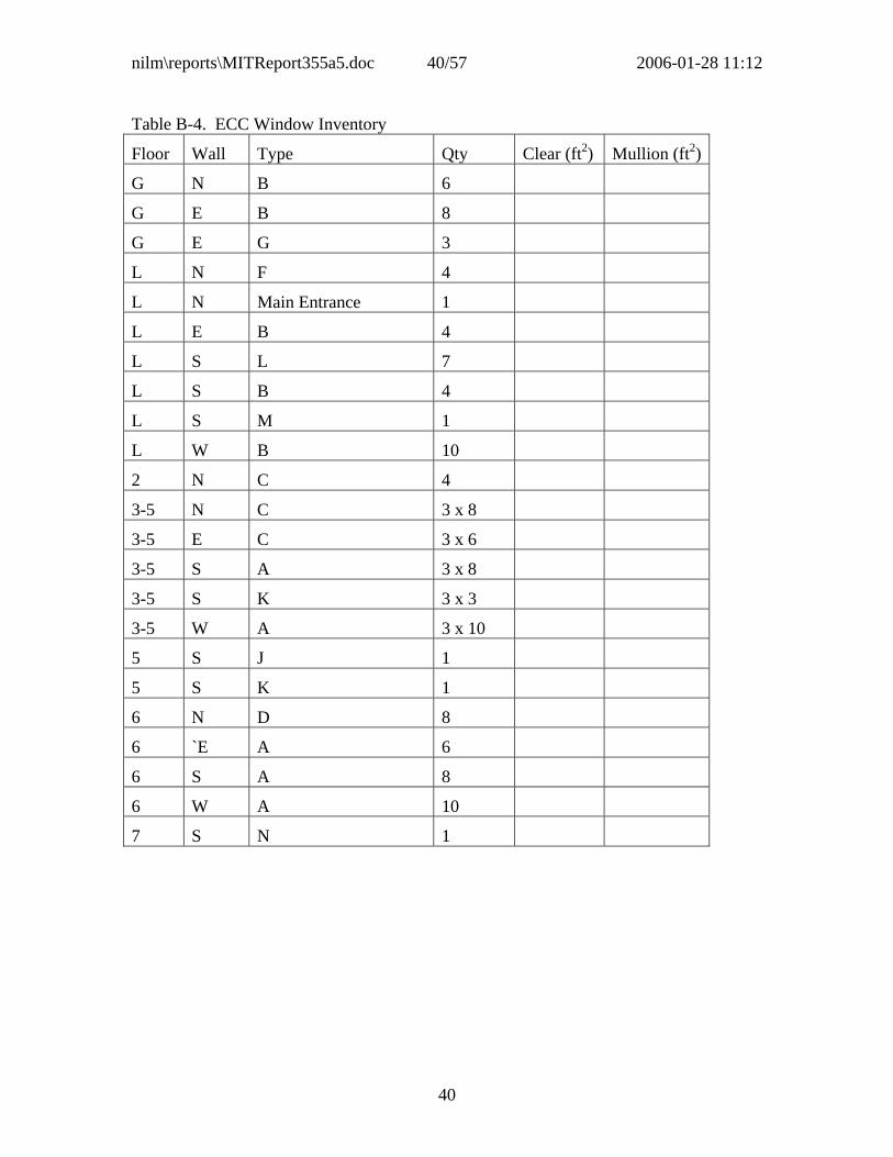
nilm\reports\MITReport355a5.doc 40/57 2006-01-28 11:12
40
Table B-4. ECC Window Inventory
Floor Wall Type Qty Clear (ft2) Mullion (ft2)
G N B 6
G E B 8
G E G 3
L N F 4
L N Main Entrance 1
L E B 4
L S L 7
L S B 4
L S M 1
L W B 10
2 N C 4
3-5 N C 3 x 8
3-5 E C 3 x 6
3-5 S A 3 x 8
3-5 S K 3 x 3
3-5 W A 3 x 10
5 S J 1
5 S K 1
6 N D 8
6 `E A 6
6 S A 8
6 W A 10
7 S N 1

nilm\reports\MITReport355a5.doc 41/57 2006-01-28 11:12
41
Table B-5. ECC Window and Wall Areas
Wall Dimensions (ft) Gross(ft2) Clear(ft2) Mullion(ft2)
N(E10)
E(N11)
N(N12)
E(E8)
S
W
Roof
ground 240x(96+12) 25,920
10 the north-facing wall of the east wing, N(E), is partly shaded at times by the north wing 11 the east-facing wall of the north wing, E(N), is partly shaded at times by the east wing 12 the end walls of the north and east wings, N(N) and E(E), are never shaded by other parts of the building
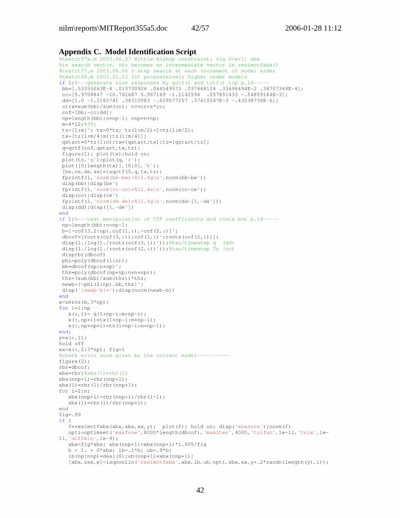
nilm\reports\MITReport355a5.doc 42/57 2006-01-28 11:12
42
Appendix C. Model Identification Script %testctf7x.m 2003.06.07 Hittle-Bishop constraint: via 0<x<1; xbx %is search vector, rbr becomes an intermediate vector in resimctfxbx() %testctf7.m 2003.06.06 2-step search at each increment of model order %testctf6.m 2003.01.12 fit progressively higher order models if 1;%---generate sine responses by qctf() and tctf() top p.14----- bb=[.53355063E-4 .013730926 .064549573 .037668124 .33696494E-2 .38707349E-4]; cc=[5.9708847 -10.761687 5.967169 -1.1142596 .057851433 -.54859184E-3]; dd=[1.0 -1.2165741 .38310083 -.029577257 .37410267E-3 -.43038736E-6]; crrx=sum(bb)/sum(cc); cc=crrx*cc; cof=[bb;-cc;dd]; np=length(bb);n=np-1; nnp=n+np; m=4*12;%30; tz=[1:m]'; tz=0*tz; tz(1:m/2)=1+tz(1:m/2); tx=[tz(1+m/4:m);tz(1:m/4)]; qstart=0*tz(1:n);tx=[qstart;tx];tz=[qstart;tz]; q=qctf(cof,qstart,tx,tz); figure(1); plot(tx);hold on; plot(tz,'g');plot(q,'r'); plot([0;length(tx)],[0;0],'k'); [be,ce,de,se]=lsqctf(5,q,tx,tz); fprintf(1,'norm(bb-be)=%11.4g\n',norm(bb-be')) disp(bb);disp(be') fprintf(1,'norm(cc-ce)=%11.4e\n',norm(cc-ce')) disp(cc);disp(ce') fprintf(1,'norm(dd-de)=%11.4g\n',norm(dd-[1,-de'])) disp(dd);disp([1,-de']) end if 1;%---test manipulation of CTF coefficients and roots bot p.14----- np=length(bb);n=np-1; b=[-cof(3,2:np),cof(1,:),-cof(2,:)]'; dbcof=[roots(cof(3,:));cof(1,:)';roots(cof(2,:))]; disp(1./log(1./roots(cof(3,:))'));%tau/timestep q (dd) disp(1./log(1./roots(cof(2,:))'));%tau/timestep Tz (cc) disprbr(dbcof) phi=poly(dbcof(1:n)); bb=dbcof(np:n+np)'; thz=poly(dbcof(np+np:n+n+np)); thz=(sum(bb)/sum(thz))*thz; newb=[-phi(2:np),bb,thz]'; disp('|newb-b|=');disp(norm(newb-b)) end x=zeros(m,3*np); for i=1:np x(:,i)= q(1+np-i:m+np-i); x(:,np+i)=tx(1+np-i:m+np-i); x(:,np+np+i)=tz(1+np-i:m+np-i); end; y=x(:,1); hold off xx=x(:,2:3*np); fig=1 %check error norm given by the correct model---------- figure(2); rbr=dbcof; xbx=rbr;%xbx(1)=rbr(1) xbx(nnp+1)=rbr(nnp+1); xbx(1)=rbr(1)/rbr(nnp+1); for i=2:n; xbx(nnp+i)=rbr(nnp+i)/rbr(i-1); xbx(i)=rbr(i)/rbr(nnp+i); end fig=.99 if 1 f=resimctfxbx(xbx,xbx,xx,y); plot(f); hold on; disp('xbxnorm');norm(f) opti=optimset('maxfune',8000*length(dbcof),'maxiter',4000,'tolfun',1e-11,'tolx',1e-11,'diffmin',1e-9); xbx=fig*xbx; xbx(nnp+1)=xbx(nnp+1)*1.005/fig b = 1. + 0*xbx; lb=.1*b; ub=.9*b; lb(np:nnp)=deal(0);ub(nnp+1)=xbx(nnp+1); [xbx,sse,e]=lsqnonlin('resimctfxbx',xbx,lb,ub,opti,xbx,xx,y+.2*randn(length(y),1));

nilm\reports\MITReport355a5.doc 43/57 2006-01-28 11:12
43
figure(3);plot(e) disp([norm(rbr-dbcof),sse,e'*e,sqrt(sse/length(e))]) rbk=xbx;%rbk(1)=xbx(1) DELETE THIS STUFF rbk(1)=xbx(1)*rbk(nnp+1); for i=2:n;rbk(nnp+i)=xbx(nnp+i)*rbk(i-1);rbk(i)=xbx(i)*rbk(nnp+i);end disprbr(rbk) e=resimctfxbx(xbx,xbx,xx,y); disp('rbr-dbcof|,sse,sse,rms=') disp([norm(rbr-dbcof),sse,e'*e,sqrt(sse/length(e))]) alle=e;figure(4);plot(e) end return function f=resimctfxbx(xbxr,xbx,x,y) %this uses past predicted y=ye; also try with past values of y data % f=resCTFrbr(rbr,x,y) returns m residuals given parm estimate, % b=[roots(phi);thx;roots(thz)], and data x(mxlen(b)),y(mx1). % Columns of x correspond to [phi',thx',thz'] elements. See testctf3 np=(length(x(1,:))+1)/3; n=np-1; nnp=n+np; if length(xbx)==length(xbxr);%for 2-step t-consts search when incrementing model order xbx=xbxr; else xbx(n-1:n)=xbxr(1:2); xbx(np:n+np)=xbxr(3:2+np); nr=length(xbxr); xbx(n+np+n-1:n+np+n)=xbxr(nr-1:nr); end rbr=xbx;%rbr(1)=xbx(1) rbr(1)=xbx(1)*rbr(nnp+1); for i=2:n; rbr(nnp+i)=xbx(nnp+i)*rbr(i-1); rbr(i)=xbx(i)*rbr(nnp+i); end dbc=[rbr;0]; p=poly(rbr(1:n)); dbc(1:n)=-p(2:np)'; p=poly(rbr(1+np+n:n+np+n)); dbc(1+np+n:np+np+n)=p'*sum(rbr(np:np+n))/sum(p); ye=0*y; ye(1)=x(1,:)*dbc; for k=2:length(y); x(k,2:n)=x(k-1,1:n-1); x(k,1)=ye(k-1); %x(k,1)=y(k-1); ye(k)=x(k,:)*dbc; end f=y-ye;

nilm\reports\MITReport355a5.doc 44/57 2006-01-28 11:12
44
Appendix D. Design Conditions and TMY Weather ASHRAE Fundamentals 1997, Chapter 26 Climatic Design Information Latitude: 33.93 Longitude: 118.4 Elevation (m): 32 Heating 99.6% (C): 6.2 Heating 99.0% (C): 7.4 Windspeed 1% (m/s): 9.2 Windspeed 2.5% (m/s): 7.9 Windspeed 5% (m/s): 7.1 Daily Max (C): 35.9 Daily Min (C): 3.5 Humid ratio 0.4% (g/kg): 14 Humid ratio 1% (g/kg): 14 Humid ratio 2% (g/kg): 13 TMY2: WBAN=23174 » tmystats Heating 99.5% (C) 7.2 Heating 99.0% (C) 7.8 Cooling 99.0% (C) 26.1 Cooling 99.5% (C) 27.2 Windspeed 1% (m/s) 11.0 Windspeed 2.5%(m/s) 7.7 Windspeed 5% (m/s) 6.7 Daily Min(C) 4.4 Daily Max(C) 35.0

nilm\reports\MITReport355a5.doc 45/57 2006-01-28 11:12
45
Appendix E. Simulation To compare cooling control strategies we must estimate annual energy use and cost for each strategy while all other aspects of building operation are held constant. These “constants” include fan and chiller performance curves; fan, chiller, and auxiliary equipment control sequences; weekly and holiday schedules that describe internal gains, minimum outside air and fan static pressure; zone temperature setpoint schedule and related control parameters; and weather.
Chiller Performance. ISD coil loads were monitored for two weeks, 29 August – 9 September, 2002, a period which included very hot weather. The total coil load is computed from its sensible, Fcp(Tcold – Tmix) and latent, Fhfg(wmix – wcold), air-side components. The measured 5-minute average sensible and total coil load are plotted in Figure E-1 against chiller power. Note that latent fraction increases moderately with load, as expected for an essentially constant air-side flow rate. Chiller specific power, expressed as chiller power per unit coil load (kW/Ton) decreases with load. This is also expected. The condenser and evaporator areas are fixed so the approach temperatures increase with load resulting in the lift temperature increasing even faster than the condenser-chilled water temperature difference. Only one chiller was operated during this period. There are four compressors per chiller and the resulting performace in each of four operational stages, clearly evident in the plot, is summarized in Table 1. Table E-1. ISD chiller performance summary for 29 August – 9 September 2002
Qtot Qtot Qlat/Qtot Pch/Qtot(kBtuh) (RefTon) (-) (kW/RT 770 64 0.28 0.52 1270 106 0.31 0.65 1500 125 0.30 0.81 1700 142 0.31 0.93
Figure E-1. Observations of ISD chiller performance (one-minute average data).
ISD 29 Aug - 9 Sep 2002
0
200
400
600
800
1000
1200
1400
1600
1800
0 10 20 30 40 50 60
Pch (kW/3)
Coi
l Loa
d (k
Btu
h)
QsenQtot
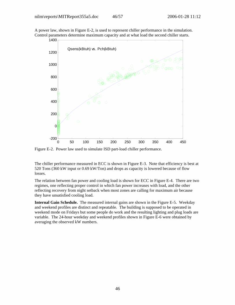
nilm\reports\MITReport355a5.doc 46/57 2006-01-28 11:12
46
A power law, shown in Figure E-2, is used to represent chiller performance in the simulation. Control parameters determine maximum capacity and at what load the second chiller starts.
Figure E-2. Power law used to simulate ISD part-load chiller performance. The chiller performance measured in ECC is shown in Figure E-3. Note that efficiency is best at 520 Tons (360 kW input or 0.69 kW/Ton) and drops as capacity is lowered because of flow losses.
The relation between fan power and cooling load is shown for ECC in Figure E-4. There are two regimes, one reflecting proper control in which fan power increases with load, and the other reflecting recovery from night setback when most zones are calling for maximum air because they have unsatisfied cooling load.
Internal Gain Schedule. The measured internal gains are shown in the Figure E-5. Weekday and weekend profiles are distinct and repeatable. The building is supposed to be operated in weekend mode on Fridays but some people do work and the resulting lighting and plug loads are variable. The 24-hour weekday and weekend profiles shown in Figure E-6 were obtained by averaging the observed kW numbers.
0 50 100 150 200 250 300 350 400 450-200
0
200
400
600
800
1000
1200
1400
Qsens(kBtuh) vs. Pch(kBtuh)

nilm\reports\MITReport355a5.doc 47/57 2006-01-28 11:12
47
Figure E-3. ECC chiller performance based on air-side sensible plus latent loads Figure E-4. Relation between fan power and coil load based on ECC data
CCt Sep 2002 (w/T&P density correction)
-100
0
100
200
300
400
500
600
700
800
0 100 200 300 400 500 600 700Input (kW)
(Cp(
Tmix
-Tsa
)+hf
g(w
mix
-wsa
))*m
dot (
~RT)
CCt Sep 2002
0
10
20
30
40
50
60
0 200 400 600 800 1000 1200 1400 1600
(Tmix-Tsa)*Psfan
Psfa
n

nilm\reports\MITReport355a5.doc 48/57 2006-01-28 11:12
48
Figure E-5. Measured hourly loads (main – HVAC) for the ISD building (kW). Figure E-6. Occupied and unoccupied internal gain schedules used for ISD simulations (kW).
0 5 10 15 20 25150
200
250
300
350
400
450
500
550
figure(3);plot(1+mod([1:477],24),x(:,8),'bo'); (Pmain-Phvac-Pmcab)
0 5 10 15 20 25200
250
300
350
400
450
500
550
figure(3);plot(1+mod([1:477],24),x(:,8),'bo'); (Pmain-Phvac-Pmcab)

nilm\reports\MITReport355a5.doc 49/57 2006-01-28 11:12
49
Control of Fan and Outside Air. The following truth table summarizes the control structures used in the simulation in a form that can be readily ported to an EMCS for a demonstration. The logical input columns (1-6) have entries of 1=true, 0=false and *=either. The zone temperature setpoint relation Tz|Te refers to the economizer set point, Te, which may be different in occupied and unoccupied periods. For example Tz<Te generally turns the fan off in unoccupied periods and reduces outside airflow to the minimum required for ventilation in occupied periods. The output columns (7-8) refer to fan and damper operation. Fnom is the nominal (maximum) supply fan mass flow rate and %F/Fnom is the fraction of Fnom expressed as a percent.
1 2 3 4 5 6 7 8 9 10 11 Occupied Night
fan Fan gain
Tz>Toa Tz|Te (1)
No econ
%F/Fnom %OA H/C SP
TQ (2)
Notes
1 * * * * 1 100 15 1 (3) 1 * * 0 * 0 100 15 1 1 * * 1 < 0 100 15 1 1 * * 1 ≥ 0 100 100 1 (4) 0 * * * * 1 0 0 2 T (3) 0 0 0 * * 0 0 0 2 T 0 1 0 0 * 0 0 0 2 T 0 1 0 1 < 0 0 0 2 T 0 1 0 1 ≥ 0 100 100 2 (4) 0 1 >0 * * 0 Illegal 2 0 0 >0 0 * 0 0 0 2 T 0 0 >0 1 < 0 0 0 2 T (5) 0 0 >0 1 ≥ 0 (6) (6) 2 T (4,6)
(1) Tz, the economizer cooling setpoint, may take different values in occupied and unoccupied periods (2) evaluate Tz when H/C setpoints are satisfied: TH < Tz < TC; else evaluate Qz unless noted otherwise in this column (3) when “NoEcon” is set we always zero “NightFan” and “FanGain” (4) when result is Tz < Te, set Tz = Te, evaluate CRTF, and reduce fan power so that airflow, F, corresponds to Qz (5) usually set Te = -99C (6) F=g*(Tz -Toa) where g is daily fan gain, the optimization variable. . CRTF for Simulation. Recall from the Envelope Response Model subsection that the discrete-time model (5) can be evaluated recursively for Qz or Tz: for Tz: ),(),(),( 1000, zz
nww
nzz
nzz TBTBQBT θθφθ −+= (7a)
that is, Tz = RHS expression divided by θz,0, and for Qz: ),(),(),( 0010, zz
nww
nzz
nzz TBTBQBQ θθφφ −+=− (8)
With φz = -1 eqn (8) becomes: ),(),(),( 001 zz
nww
nzz
nz TBTBQBQ θθφ −+= (9)
When the zone heat balance involves exchange of outside air, i.e.,
Qz = Fcp(Tz – Toa) - Qstar, where Qstar = Qh/c + Qsolrad + Qig, the expression for Tz becomes:
pz
zzn
wwn
zzn
otherpz Fc
TBTBQBQFcT
+
−+++=
0,
101 ),(),(),(θ
θθφ (7b)
and it is easy to see that with F = 0, (7b) reduces to (7a).

nilm\reports\MITReport355a5.doc 1/57 2006-01-28 11:12
1
Setpoint Control. Zone temperature control can be implemented in a number of ways such as single- or multi-stage on-off control, continuous (heating and cooling) throttling range, and throttling ranges separated by deadbands. The latter, with capacity limits placed on each throttling band, is the most general because it can emulate multi-stage on-off control if the throttling ranges are made very stiff while also able to emulate continuous throttling if both heating and cooling capacity are modulated inversely over the same throttling range. Throttling bands are commonly defined in advance by means of software or hardware settings. The band settings may be arranged to change on a predetermined schedule, e.g. one set of throttling ranges in occupied mode and another set in unoccupied mode. Such predifined zone temperature bands can be augmented by special breakpoints, for example the point at which zone temperature (enthalpy) crosses outside temperature (enthalpy) is a key parameter for economizer control. Thus a typical zone control might have four zone temperature breakpoints, TH < TE < TO < TC, and four corresponding plant capacities, QH > 0 > QE > QC; capacity is controlled as follows: TZ < TH Q = QH TZ = TH 0 < Q < QH TH < TZ < TE Q = 0 TZ = TE QE(TE) < Q < 0 TE < TZ < TO Q = QE(TZ) TZ = TO Q = 0 TE < TZ < TC Q = QE(TZ) TZ = TC QE(TC) + QC < Q < QE(TC) TC < TZ Q = QE(TZ) + QC TE < TZ < TC Q = QE(TZ) TZ = TC QE(TC) + QC < Q < QE(TC) TC < TZ Q = QE(TZ) + QC (Note that QC1 = -F(TC1 - TOA)+, i.e., economizer cooling capacity at 100%OA with TZ = TC1, or zero, whichever is less, and QC2 = -F(TC2 - TOA)+ plus the capacity of the highest stage of mechanical cooling.) The new CRTF heat rate and temperature (Qz, Tz) are evaluated at each timestep by applying the plant capacities progressively starting with QC2:

nilm\reports\MITReport355a5.doc 2/57 2006-01-28 11:12
2
Setpoint Control. There are four zone setpoints, TH2 < TH1 < TC1 < TC2, and four corresponding maximum plant capacities, QH2 > QH1 > 0 > QC1 > QC2. (Note that QC1 = -F(TC1 - TOA)+, i.e., economizer cooling capacity at 100%OA with TZ = TC1, or zero, whichever is less, and QC2 = -F(TC2 - TOA)+ plus the capacity of the highest stage of mechanical cooling.) The new CRTF heat rate and temperature (Qz, Tz) are evaluated at each timestep by applying the plant capacities progressively starting with QC2: Tz = CRTF(QC2, Fmax); if Tz < TC2 QC = CRTF(TC2); Tz = TC2 if QC > QC12 Tz = CRTF(QC1, Fmax) if Tz < TC1 QC = CRTF(TC1); F=Fmax)*QC/QC, if QC > QC2 Tz = CRTF(QC1, Fmax) if Tz < TC1 QC = CRTF(TC1); F=Fmax)*QC/QC, … As soon as the bracketing setpoints have been found, the progression can be terminated and the heat balance solved for Tz.: QCRTF + QH + QC + QE + QIG + QSR = 0 where QCRTF = θxoTx - θzoTz + QP, and QE = GE(Tx - Tz). Zone temperature is thus evaluated by: Tz = ((GE + θxo)Tx + QP + QH + QC + QIG + QSR)/(GE + θzo) TQ: The interval in which Tz = Tx is a special case in which the heat balance is quadratic, rather than linear: sting…

nilm\reports\MITReport355a5.doc 3/57 2006-01-28 11:12
3
Control Parameters. Eight control logic sequences are defined in order to explore the extent to which simple control tactics can approach the optimal13. We consider the following free cooling control cases: 0) none, 1) actual, 2) standard, 3) Lower day setpoint, 4) Night precooling, 5) Lower night setpoint, 6) cases 3 and 5 combined, 7) case 6 augmented by chiller on hot nights. Fans run continuously during occupied hours and as needed (cases 4-7) to satisfy night setpoint. The effects of pressure drop and fan efficiency are assessed in the post processor by taking the product of annual air volume and specific fan power. The main simulation needs to integrate air flow separately for day and night operation so that we can consider the case of opening windows and using the return fan only (e.g. tasking janitors to open all windows “x inches” at night; e-mailing occupants in day to act as online forecast/simulation results dictate...with some flexibility for personal comfort). Probably useful to track day and night H/C loads separately as well. Cases with reduced free cooling setpoint (3-7) can benefit from online forecast/response prediction/optimal control. Daily prediction of heating/cooling needs (internal and solar gains; outside air and CRTF loads) is basic to this control improvement. For discrete-state/schedule-based control we assign control parameters for the eight cases as follows. The cooling setpoints are Tm for mechanical cooling and Te for economizer cooling. Subscript “o” is for occupied hours; subscript “n” is for unoccupied hours. case
Night fan enable
fOA econ
Tecon enable
Tz2o
Tz2n
Tz1o
Tz1n
0 none 0 0 -99 74 74 74 199 1 actual 0 .7 65 74 74 74 199 2 ideal 0 1.0 199 74 74 74 199 3 lower day sp 0 1.0 199 68 74 74 199 4 night=day sp 1 1.0 199 74 74 74 199 5 lower night sp 1 1.0 199 74 68 74 199 6 (3 + 5) 1 1.0 199 68 68 74 199 7 (6+night chlr) 1 1.0 199 68 68 74 74
13 Free cooling potential is a function of climate (diurnal and seasonal temperature and solar radiation) and plant (slow, medium, and fast mass, solar aperture/orientation, internal gain cycles, fan and chiller power), as well as control strategy.

nilm\reports\MITReport355a5.doc 4/57 2006-01-28 11:12
4
Appendix F. Electric Rate Structure The incremental cost of a change in HVAC control cannot be determined independent of other building loads because of the utility rate structure. A cost algorithm therefore has to be built into the simulation (as well as any practical real world implementation) that models optimal control. The code and test results (Figures F-1 and F-2) are documented below. Function elecbill accepts a vector of 8760 hourly at-the-meter loads, the start and end times of the billing period of interest, and the rate parameters. Two values are returned: annual energy cost and an array of the hourly demand charges that determine annual cost of peak demands by rate bin. The first array index is the month and the second is the time-of-use index keyed to the time-of-use periods defined by the 168-hour rate schedule array: 1=off-peak, 2=mid-peak and 3=on-peak. Note that the various control objective functions generally ignore the annual ratchet charge and only penalize daily demand cost when it exceeds the monthly baseline. Each day we minimize (cost of energy) + xd(off) + xd(mid) + xd(peak) + xd(rat) where x∈[off,mid,peak,rat] and xd(x) is rate(x)*(demand(x) in excess of monthly baseline demand(x)). {This attempts to handle the possibility that the baseline peaks may occur on different days; if not, it simplifies to: minimize (cost of energy) + (excess demand cost) where (excess demand cost) = sumx(rate(x)*demand(x)) – baseline(sumx(rate(x)*demand(x)))}. We use the fan-enabled baseline under the assumption that it will have the lower peak-period demand and thus the lower sumx. An alternative is to let xd(x) be lesser of the two baseline demand components. %testElecBill.m 20021222pra rate=struct('kwh',[.08944,.12141,.12141;.08828,.10917,.19564],'kw',[0,0,0;0,2.7,17.95]); rate.kwh rate.kw rat.chg=6.60; rat.f=.5; sced(1:24*7) = 1; sced(9:23) = 2; sced(13:18) = 3; sced(73:96) = sced(1:24); sced(97:120) = sced(1:24); sced(121:144)= sced(1:24); sced(145:168)= sced(1:24); dlsavings=0;%WINTER for i=1:168 p(1:8760)=0; p(i)=1; [ann(i),kwm]=elecbill(p,[1 168],rate,sced,rat); kwc1(i)=kwm(1,sced(i)); end; subplot(3,1,1);plot(ann);ylabel('Use+Dmd') title('Cost per kWh on given hour of the week in Winter') for i=1:168 p(1:8760)=0; p(i)=1; [ann(i),kwp,kwr(i)]=elecbillkwh(p,[1,168],rate,sced,rat); kwc2(i)=kwp(sced(i)); end; subplot(3,1,2);plot(ann);ylabel('Use Only') subplot(3,1,3);plot(kwc1,'b');hold on plot(kwc2,'rx');hold off; ylabel('Dmd Only') figure dlsavings=1;%SUMMER for i=1:168 p(1:8760)=0; if mean(p)~=0; disp(max(p)); end; p(4800+i)=1; ann(i)=0; [ann(i),kwm]=elecbill(p,[4801 4968],rate,sced,rat); %note 181*24 < 4800+i <= 212*24 therefore m=7 kwc1(i)=kwm(7,sced(1+mod(4799+i+dlsavings,24*7))); end; subplot(4,1,1);plot(ann);ylabel('Use+Dmd') title('Cost per kWh on given hour of the week in Summer') for i=1:168 p(1:8760)=0; p(4800+i)=1;
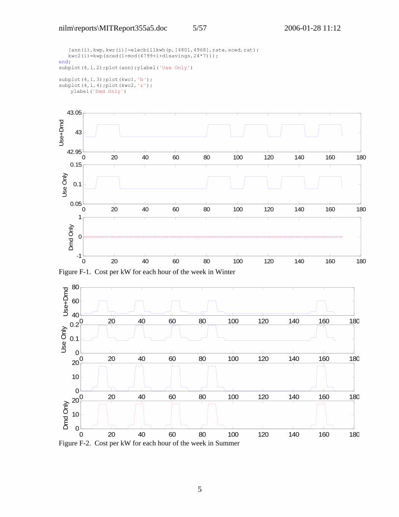
nilm\reports\MITReport355a5.doc 5/57 2006-01-28 11:12
5
[ann(i),kwp,kwr(i)]=elecbillkwh(p,[4801,4968],rate,sced,rat); kwc2(i)=kwp(sced(1+mod(4799+i+dlsavings,24*7))); end; subplot(4,1,2);plot(ann);ylabel('Use Only') subplot(4,1,3);plot(kwc1,'b'); subplot(4,1,4);plot(kwc2,'r'); ylabel('Dmd Only')
0 20 40 60 80 100 120 140 160 18042.95
43
43.05
Use
+Dm
d
0 20 40 60 80 100 120 140 160 1800.05
0.1
0.15
Use
Onl
y
0 20 40 60 80 100 120 140 160 180-1
0
1
Dm
d O
nly
Figure F-1. Cost per kW for each hour of the week in Winter
0 20 40 60 80 100 120 140 160 18040
60
80
Use
+Dm
d
0 20 40 60 80 100 120 140 160 1800
0.1
0.2
Use
Onl
y
0 20 40 60 80 100 120 140 160 1800
10
20
0 20 40 60 80 100 120 140 160 1800
10
20
Dm
d O
nly
Figure F-2. Cost per kW for each hour of the week in Summer

nilm\reports\MITReport355a5.doc 6/57 2006-01-28 11:12
6
Appendix G. Optimization Algorithms Cases 11-15 of the economizer and precooling controls study use a variable duration of night ventilation to reduce night fan energy consumption, relative to cases 6-10, in which the fan runs at night whenever the indoor-outdoor temperature difference is positive. The algorithm for determining start time each night is suboptimal in the sense that it minimizes electric cost each day without considering the effect, assumed to be small, on subsequent days.
The assertion that this effect is small is based on the following reasoning. On warm days, precooling will delay the chiller start time but the thermal state at the end of occupancy will be nearly the same regardless of the amount of precooling. On cool days the chiller will not come on and the zone temperature will usually not rise above the economizer set point so, again, the thermal state at the end of occupancy will be little influenced by the amount of precooling. On mild days (when zone temperature rises above the economizer setpoint but does not reach the mechanical cooling set point until late in the day, if at all) the average temperature of thermal mass may depend appreciably on the amount of precooling; however mild days are usually followed by cool nights in which the amount of fan energy for a given amount of precooling is small.
Because thermal response is modeled in discrete time with one hour time steps, the optimal start time must be one of the (usually 12 to 14) unoccupied hours or the first occupied hour if the optimal duration is zero. It is no great computational burden to solve this such an optimization problem by complete enumeration, i.e. by testing all possible start times, i=1:n+1, where n is the number of unoccupied hours as follows.
1) simulate from the last occupied hour to the ith unoccupied hour with the fan off;
2) simulate hours i+1:n with the fan on;
3) simulate occupied hours in the usual way with fan on and chiller only as needed.
After recording the daily cost for all i=1:n+1, the least-cost value of i is selected and the three steps are repeated to obtain the final daily state. The foregoing process is repeated for each day of the year in sequence, d=1:365.
The computations can be reduced if it is assumed, as is reasonable, that daily cost will drop monotonically up to the least cost value of i and then increase monotonically. Under this assumption the search can stop at the first value of i that has a higher cost than the previous value and the process repeated for the previous value before moving on to the next day.
With tempering, two monotonic searches are nested for each day. At each value of i, the number of tempering hours, j, is incremented j=0, 1, … until cost stops decreasing and the minimum-cost thus found is associated with the ith fan start time. The least cost value of i is then found just as outlined previously.