project clarity 2015 annual monitoring report … project clarity 2015 annual monitoring report...

1

PROJECT CLARITY 2015 Annual Monitoring Report

(Dec. 2014 – Nov. 2015)

JANUARY 2016

Michael Hassett Maggie Oudsema

Alan Steinman, Ph.D.

Annis Water Resources Institute Grand Valley State University

Muskegon, MI 49441

2

1. Overview

Project Clarity is a large-scale, multidisciplinary, collaborative watershed remediation project aimed at improving water quality in Lake Macatawa. A holistic approach that includes wetland restoration, in-stream remediation, Best Management Practices (BMPs), and community education is being implemented by a diverse and dedicated team in a public-private partnership. Once watershed remediation is complete, the project is expected to have many economic, social, and ecological benefits – while achieving the ultimate goal of improved water quality in Lake Macatawa.

Lake Macatawa is the terminus of a highly degraded watershed and has exhibited the symptoms of a hypereutrophic lake for more than 40 years (MWP 2012, Holden 2014). Extremely high nutrient and chlorophyll concentrations, excessive turbidity, low dissolved oxygen, and a high rate of sediment deposition make it one of the most hypereutrophic lakes in Michigan (MWP 2012, Holden 2014). Nonpoint source pollution from the watershed, particularly agricultural areas, is recognized as the primary source of the excess nutrients and sediment that fuel hypereutrophic conditions in Lake Macatawa (MWP 2012).

Because of this nutrient enrichment, Lake Macatawa and all of its tributaries are included on Michigan’s 303(d) list of impaired water bodies, prompting the issuance of a phosphorus Total Maximum Daily Load (TMDL) for Lake Macatawa in 2000. The TMDL set an interim target total phosphorus (TP) concentration of 50 μg/L in Lake Macatawa (Walterhouse 1999). In recent years, monthly average TP concentrations were greater than 125 μg/L, and at times exceeded 200 μg/L (Holden 2014). Thus, meeting the TMDL target represents a major challenge for the Macatawa watershed. The TMDL estimated that it would require a 72% reduction in phosphorus loads from the watershed (Walterhouse 1999). Through remediation projects and BMPs focused on key areas in the watershed, Project Clarity is focused on reducing P loads and working to meet the TMDL target for Lake Macatawa.

The Annis Water Resources Institute (AWRI) at Grand Valley State University, in cooperation with the Outdoor Discovery Center Macatawa Greenway (hereafter, ODC), is working on a long-term monitoring initiative in the Lake Macatawa watershed. The study will provide critical information on the performance of restoration projects that are part of Project Clarity, as well as the water quality status of Lake Macatawa. The goal of the monitoring effort is to measure pre- and post-restoration conditions in the watershed, including Lake Macatawa. This report documents AWRI’s monitoring activities in 2015, which represent pre-restoration conditions in combination with data reported previously from 2013-2014. Although it will take a number of years before the benefits of restoration actions in the watershed are expressed in the lake, these initial results will establish the baseline conditions against which we can assess future changes, similar to what is being done in Muskegon Lake (cf. Steinman et al. 2008; Bhagat and Ruetz 2011).

3

2. Methods

2.1 Overall site description

The Macatawa watershed (464 km2/114,000 acres) is located in Ottawa and Allegan Counties and includes Lake Macatawa, the Macatawa River, and many tributaries. It is dominated by agricultural (46%) and urban (33%) land uses, which have accounted for the loss of 86% of the watershed’s natural wetlands (MWP 2012). The watershed includes the Cities of Holland and Zeeland and parts of 13 townships (MWP 2012). Lake Macatawa is a 7.2 km2/1,780 acre drowned river mouth lake. It is relatively shallow, with an average depth of 3.6 m/12 ft and a maximum depth of 12 m/40 ft in the western basin. The Macatawa River, the main tributary to the lake, flows into the lake’s shallow eastern basin. A navigation channel in the western end of the lake connects Lake Macatawa with Lake Michigan.

AWRI’s monitoring initiative is focused on 1) two key wetland restoration areas in the Macatawa watershed (Figures 1, 2) and 2) Lake Macatawa (Figure 3). Details on these two efforts are provided below.

2.2 Wetland Restoration: Middle Macatawa & Haworth Properties

2.2.1 Monitoring & Data Collection

Two wetland properties were acquired as part of Project Clarity and were designated as the Middle Macatawa and Haworth properties. Restored wetlands on the properties were designed to slow the flow of water in the Macatawa River and its tributaries, particularly during high flow events, thus trapping and retaining suspended sediments and nutrients. Restoration construction at Middle Macatawa and Haworth was completed in late September and early October 2015, respectively.

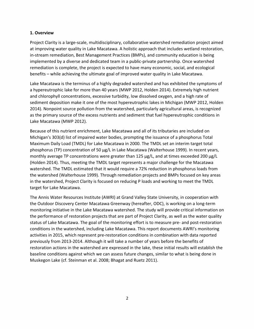
Both properties have sampling sites located upstream and downstream of the restoration area. The Middle Macatawa study area (Figure 1) has two upstream sites (Macatawa River and Peter’s Creek, which flow into the Macatawa River) and two downstream sites (Macatawa River at the USGS gauging station [Macatawa Down USGS] and at Adams Street Landing [Macatawa Down Adams]). Sampling at Adams Street Landing was discontinued in March 2015 due to concerns that the Adams sampling site was too far downstream from the restoration area (~1.5 river miles) to accurately reflect the effect of restoration, so it was not included in statistical analysis in 2015. The Haworth study area (Figure 2) consists of sampling locations upstream and downstream of the restoration area, on the North Branch of the Macatawa River.

Water quality and hydrologic monitoring are ongoing and this report includes data from December 2014 through November 2015. Sampling occurred monthly during base flow conditions and during 1 storm event (~≥ 0.5 inches of rain proceeded by 72 hours of dry weather; Table 1). During each monitoring event, general water quality parameters (dissolved oxygen [DO], temperature, pH, specific conductivity, total dissolved solids [TDS], redox potential [ORP], and turbidity) were measured using a YSI 6600 sonde. Grab samples were collected for analysis of phosphorus (soluble reactive phosphorus [SRP], total phosphorus [TP]) and nitrogen (ammonia [NH3], nitrate [NO3], and total Kjeldahl nitrogen [TKN]) species. All water quality measurements and sample collection took place in the thalweg of the channel at permanently-established transects. Duplicate water quality

4

samples and sonde measurements were taken every other month during base flow conditions and the storm event. All samples were placed in a cooler on ice until received by the AWRI lab, usually within 4 hours, where they were stored and processed appropriately.

Water for SRP and NO3 analysis was syringe-filtered through 0.45-μm membrane filters into scintillation vials and frozen until analysis. NH3 and TKN were acidified with sulfuric acid and kept at 20°C until analysis. SRP, TP, NH3, NO3, and TKN were analyzed on a SEAL AQ2 discrete automated analyzer (U.S. EPA 1993). Any values below detection were calculated as ½ the detection limit.

Stream hydrographs were installed at each monitoring location. Water level loggers and staff gauges were installed at permanently-established transects at each of the 6 monitoring locations. Manual water velocity (using a Marsh McBirney Flow-mate 2000) and stage measurements were taken at each transect during each baseflow sampling event and over a range of high flow conditions to develop stage-pressure, stage-discharge, and pressure-discharge relationships. We anticipate having sufficient high flow measurements by summer of 2016 to develop the discharge models. Once calibrated, these models will be applied to the high-frequency pressure data recorded by the water level loggers to develop a stream hydrograph at each location (Chu and Steinman 2009).

Figure 1. The Middle Macatawa wetland restoration study area. Sampling locations (n=4), located on Peter’s Creek and the Macatawa River, are indicated with red dots. Sampling at Adams Street Landing was discontinued in March 2015 (see text for details).

Suspended sediment load associated with high flow events was quantified using PVC sediment collection tubes, which were designed and used by Hope College in previous studies in the Macatawa watershed. Sediment collection tubes were installed near each of the monitoring locations. Sediment samples were collected from the tubes after each high flow event, defined when the USGS gauge station on the Macatawa River reaches 300 cfs, and processed by ODC

5

and/or Hope College staff. The suspended sediment load results will be reported separately by the ODC.

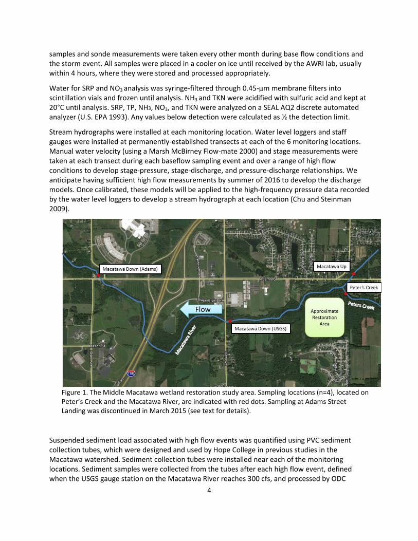
Turbidity sensors (YSI 600OMS V2) were deployed at the upstream and downstream locations on the main branch of the Macatawa River before snowmelt in April 2015. The sensors log turbidity measurements every 30 minutes. These sensors will complement the sediment load data obtained from the passive PVC sediment sampler tubes, capturing smaller storm events and base flow events. The turbidity sensors were removed in December 2015 to avoid possible ice damage and will be returned to their former locations before the snowmelt in the spring of 2016.

Figure 2. The Haworth wetland restoration study area. Sampling locations (n=2), located on the North Branch of the Macatawa River, are indicated with red dots.

2.2.2 Data Analysis Because wetland restoration was completed only in September and October 2015, we cannot rigorously compare pre vs. post-restoration differences. Rather, our analysis focuses on characterizing water quality at the two properties, and identifying 1) upstream-downstream differences and 2) baseflow-storm flow differences in nutrients and turbidity. Identification of any patterns prior to restoration will aid in distinguishing restoration effects from inherent variability in the future.

Upstream-downstream differences between site pairs (e.g., Macatawa Up vs. Macatawa Down [USGS]) were statistically tested using either a two-tailed paired t-test (normally-distributed data) or Wilcoxon signed rank test (non-normally distributed data). Baseflow vs. storm flow conditions was not statistically tested in 2015 due to the insufficient number of storm sampling events (n = 1). Normality was tested using the Shapiro-Wilk test and equal variance was tested using the Brown-

6

Forsythe test. Statistical significance was indicated by p-values < 0.05. All statistical tests were performed using SigmaPlot 13.0.

2.3 Lake Macatawa: Long-Term Monitoring

Water quality monitoring was conducted at 5 sites during spring, summer, and fall 2015 (Figure 3). The sampling sites correspond with Michigan Department of Environmental Quality (MDEQ) monitoring locations to facilitate comparisons with recent and historical data. At each sampling location, general water quality measurements (DO, temperature, pH, specific conductivity, TDS, ORP, turbidity, chlorophyll a, and phycocyanin [cyanobacterial pigment]) were taken using a YSI 6600 sonde at the surface, middle, and near bottom of the water column. Water transparency was measured as Secchi disk depth. Water samples were collected from the surface and near-bottom of the water column using a Van Dorn Bottle and analyzed for SRP, TP, and chlorophyll a. Samples also were taken for phytoplankton community composition and archived for possible future analysis.

Water for SRP analysis was syringe-filtered through 0.45-μm membrane filters into scintillation vials and frozen until analysis. SRP and TP were analyzed as previously described. Chlorophyll a samples were filtered through GFF filters and frozen until analysis on a Shimadzu UV-1601 spectrophotometer (APHA 1992).

The fish community was sampled in fall 2015. A full report on this effort is included in Appendix A.

Our pre-restoration analysis of lake monitoring data is focused on characterizing the water quality status of the lake, including comparisons to established water quality targets, and identification of seasonal trends. Understanding and documenting these baseline characteristics will facilitate the detection of future changes due to restoration.

Figure 3. Map of Lake Macatawa showing the 5 sampling locations (green dots) for long-term water quality monitoring.

7

3. Results

3.1 Wetland Restoration: Middle Macatawa Property

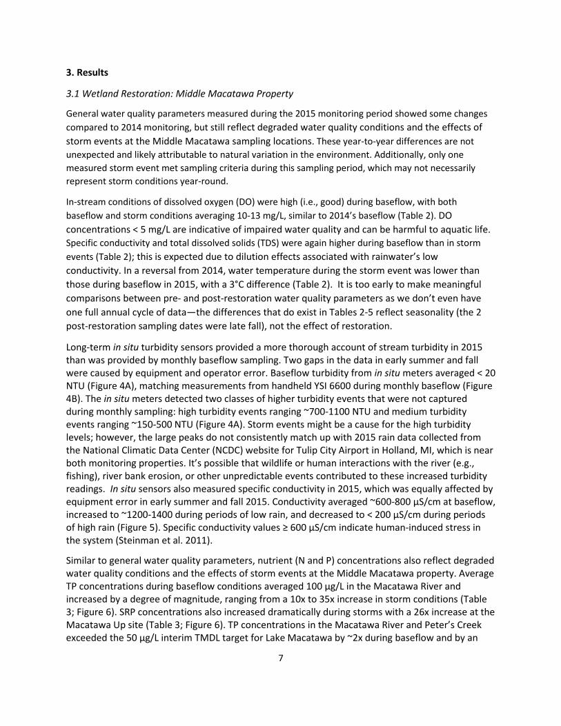
General water quality parameters measured during the 2015 monitoring period showed some changes compared to 2014 monitoring, but still reflect degraded water quality conditions and the effects of storm events at the Middle Macatawa sampling locations. These year-to-year differences are not unexpected and likely attributable to natural variation in the environment. Additionally, only one measured storm event met sampling criteria during this sampling period, which may not necessarily represent storm conditions year-round.

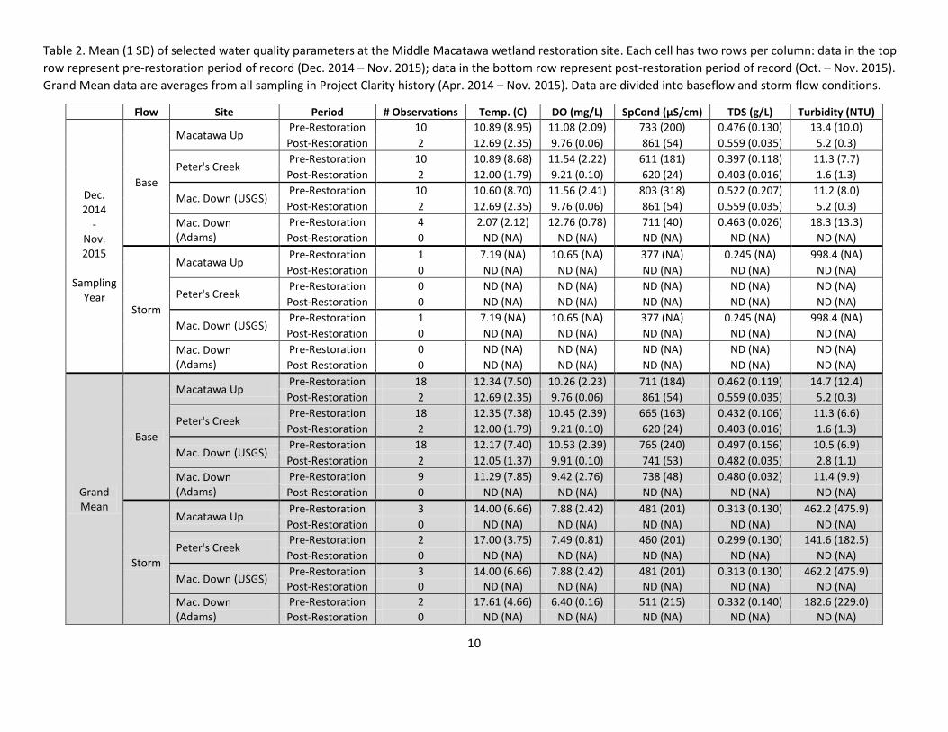
In-stream conditions of dissolved oxygen (DO) were high (i.e., good) during baseflow, with both baseflow and storm conditions averaging 10-13 mg/L, similar to 2014’s baseflow (Table 2). DO concentrations < 5 mg/L are indicative of impaired water quality and can be harmful to aquatic life. Specific conductivity and total dissolved solids (TDS) were again higher during baseflow than in storm events (Table 2); this is expected due to dilution effects associated with rainwater’s low conductivity. In a reversal from 2014, water temperature during the storm event was lower than those during baseflow in 2015, with a 3°C difference (Table 2). It is too early to make meaningful comparisons between pre- and post-restoration water quality parameters as we don’t even have one full annual cycle of data—the differences that do exist in Tables 2-5 reflect seasonality (the 2 post-restoration sampling dates were late fall), not the effect of restoration.

Long-term in situ turbidity sensors provided a more thorough account of stream turbidity in 2015 than was provided by monthly baseflow sampling. Two gaps in the data in early summer and fall were caused by equipment and operator error. Baseflow turbidity from in situ meters averaged < 20 NTU (Figure 4A), matching measurements from handheld YSI 6600 during monthly baseflow (Figure 4B). The in situ meters detected two classes of higher turbidity events that were not captured during monthly sampling: high turbidity events ranging ~700-1100 NTU and medium turbidity events ranging ~150-500 NTU (Figure 4A). Storm events might be a cause for the high turbidity levels; however, the large peaks do not consistently match up with 2015 rain data collected from the National Climatic Data Center (NCDC) website for Tulip City Airport in Holland, MI, which is near both monitoring properties. It’s possible that wildlife or human interactions with the river (e.g., fishing), river bank erosion, or other unpredictable events contributed to these increased turbidity readings. In situ sensors also measured specific conductivity in 2015, which was equally affected by equipment error in early summer and fall 2015. Conductivity averaged ~600-800 µS/cm at baseflow, increased to ~1200-1400 during periods of low rain, and decreased to < 200 µS/cm during periods of high rain (Figure 5). Specific conductivity values ≥ 600 μS/cm indicate human-induced stress in the system (Steinman et al. 2011).

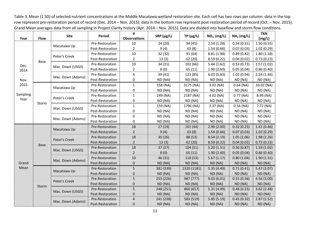
Similar to general water quality parameters, nutrient (N and P) concentrations also reflect degraded water quality conditions and the effects of storm events at the Middle Macatawa property. Average TP concentrations during baseflow conditions averaged 100 μg/L in the Macatawa River and increased by a degree of magnitude, ranging from a 10x to 35x increase in storm conditions (Table 3; Figure 6). SRP concentrations also increased dramatically during storms with a 26x increase at the Macatawa Up site (Table 3; Figure 6). TP concentrations in the Macatawa River and Peter’s Creek exceeded the 50 μg/L interim TMDL target for Lake Macatawa by ~2x during baseflow and by an

8

alarming 63x (3175 µg/L) during the April 2015 storm at the Macatawa Up site (Table 3, Figure 6). No clear upstream-downstream differences in P concentrations emerged during the 2015 monitoring period (Table 3; Figure 6), as expected given the limited post-restoration sampling.

Nitrogen concentrations also were high at the Middle Macatawa property during the 2015 monitoring period (Table 3; Figure 7). The natural level of nitrate in surface water is typically low (less than 1 mg/L); excess nitrates can result in hypoxia (low levels of dissolved oxygen) and can become toxic to warm-blooded animals at higher concentrations (10 mg/L) under certain conditions. Average nitrate concentrations exceeded 3 mg/L in Peter’s Creek and the Macatawa River during both baseflow and storm conditions (Table 3). Peter’s Creek had significantly greater nitrate than the Macatawa River sites during baseflow (p < 0.05), with concentrations averaging 8-10 mg/L during all but December and January baseflow events and the 9 April 2015 storm (Figures 7A, 7B). Consistent with the 2014 data, average nitrate concentrations continued to be greater at the Macatawa River downstream sites than at the Macatawa Up site (Table 3, Figures 7A, 7B), suggesting an impact from Peter’s Creek. In 2015, nitrate concentrations at Peter’s Creek were significantly greater than both Macatawa Up and Macatawa Down (USGS) (p < 0.001 and p = 0.017, respectively), while Macatawa Up and Down (USGS) sites were marginally different from each other (p = 0.070).

Ammonia levels of 0.1 mg/L usually indicate polluted surface waters, whereas concentrations > 0.2 mg/L can be toxic for some aquatic animals (Cech 2003). All ammonia concentrations measured at the Middle Macatawa sites were ≥ 0.1 mg/L and most were ≥ 0.2 mg/L (Figure 7C), although this could be due to sudden increase in NH3 concentration observed in November 2014 (> 8 mg NH3/L in fall 2014, Figure 7D); this increase was not observed in 2015. There were no statistically significant upstream-downstream differences in ammonia or TKN concentrations at the Middle Macatawa sites. Nitrogen concentrations were influenced by high flow conditions, but not to the degree that was observed with P (Table 3). Ammonia and TKN were higher during the 9 April 2015 storm event than baseflow at Macatawa sites, with a 7x increase from baseflow at Macatawa Up to reach ~10 mg TKN/L (Table 3, Figures 7D, 7F).

3.2 Wetland Restoration: Haworth Property

General water quality parameters measured in the North Branch at the Haworth property showed impacts similar to those observed at the Middle Macatawa property. DO concentrations again were indicative of healthy conditions, although the 9 April 2015 storm event did result in a slight decline to DO (Table 4). Specific conductance averaged 845 μS/cm during baseflow, but decreased during storms due to dilution from rainwater (Table 4). Average turbidity was low (< 6 NTU) at both Haworth sites during baseflow, but increased greatly during storms at both sites, with turbidity greater than 300 NTU, and a maximum storm turbidity increase of 77x baseflow at the North Up site (Table 4). There were no statistically significant upstream-downstream differences in turbidity at the Haworth site.

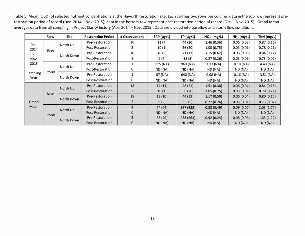
Phosphorus concentrations in the North Branch at the Haworth property were indicative of a moderately nutrient-enriched system, with average baseflow TP concentrations of ~45 μg/L (Table 5, Figure 7C). TP concentrations greatly increased at the upstream and downstream sites during the 9 April 2015 storm event with a 14x to 21x increase from baseflow and maximum concentration of

9

969 μg/L at the North Up site (Table 5, Figure 5D). SRP concentrations averaged 10 μg/L at the Haworth sites throughout the monitoring period and increased 8x-10x during stormflow, with concentrations ranging 87-115 μg/L (Figure 5B). There were no statistically significant differences in baseflow vs. storm flow P concentrations at either Haworth site.

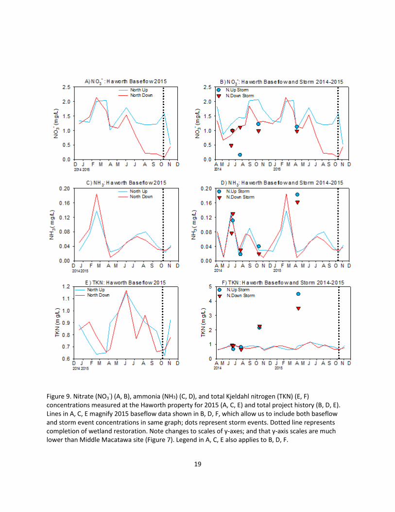
Nitrogen enrichment was less problematic at the Haworth property than at the Middle Macatawa property. Average nitrate concentrations were lower than we measured at Middle Macatawa during baseflow (Table 5). Sampling in 2014 found that nitrate at the Haworth sites was lower during storms than during baseflow, contrary to Middle Macatawa sites, but the 9 April 2015 storm only slightly decreased nitrate concentrations (Table 5, Figure 9B). Average ammonia concentrations were low (≤ 0.06 mg/L) (Table 5), but increased to 0.18 mg/L at the North Up site during the April 2015 storm (Figure 9D). TKN maintained its 2014 average into 2015; however, TKN concentrations increased greatly during storms and surpassed 2014 storm concentrations, reaching 3.5-4.5 mg/L (Figure 9D). As previously seen in 2014, the only statistically significant upstream-downstream difference in 2015 N concentrations was found for nitrate, which was greater at the upstream than at the downstream site (p = 0.0278) (Table 5).

Table 1. Precipitation summary for the storm event measured in 2015.

4/9/15

Rainfall (in) 2.03 Duration (h) 16:19 Intensity (in/h) 0.01

10

Table 2. Mean (1 SD) of selected water quality parameters at the Middle Macatawa wetland restoration site. Each cell has two rows per column: data in the top row represent pre-restoration period of record (Dec. 2014 – Nov. 2015); data in the bottom row represent post-restoration period of record (Oct. – Nov. 2015). Grand Mean data are averages from all sampling in Project Clarity history (Apr. 2014 – Nov. 2015). Data are divided into baseflow and storm flow conditions.

Flow Site Period # Observations Temp. (C) DO (mg/L) SpCond (µS/cm) TDS (g/L) Turbidity (NTU)

Dec. 2014

- Nov. 2015

Sampling

Year

Base

Macatawa Up Pre-Restoration 10 10.89 (8.95) 11.08 (2.09) 733 (200) 0.476 (0.130) 13.4 (10.0) Post-Restoration 2 12.69 (2.35) 9.76 (0.06) 861 (54) 0.559 (0.035) 5.2 (0.3)

Peter's Creek Pre-Restoration 10 10.89 (8.68) 11.54 (2.22) 611 (181) 0.397 (0.118) 11.3 (7.7) Post-Restoration 2 12.00 (1.79) 9.21 (0.10) 620 (24) 0.403 (0.016) 1.6 (1.3)

Mac. Down (USGS) Pre-Restoration 10 10.60 (8.70) 11.56 (2.41) 803 (318) 0.522 (0.207) 11.2 (8.0) Post-Restoration 2 12.69 (2.35) 9.76 (0.06) 861 (54) 0.559 (0.035) 5.2 (0.3)

Mac. Down (Adams)

Pre-Restoration 4 2.07 (2.12) 12.76 (0.78) 711 (40) 0.463 (0.026) 18.3 (13.3) Post-Restoration 0 ND (NA) ND (NA) ND (NA) ND (NA) ND (NA)

Storm

Macatawa Up Pre-Restoration 1 7.19 (NA) 10.65 (NA) 377 (NA) 0.245 (NA) 998.4 (NA) Post-Restoration 0 ND (NA) ND (NA) ND (NA) ND (NA) ND (NA)

Peter's Creek Pre-Restoration 0 ND (NA) ND (NA) ND (NA) ND (NA) ND (NA) Post-Restoration 0 ND (NA) ND (NA) ND (NA) ND (NA) ND (NA)

Mac. Down (USGS) Pre-Restoration 1 7.19 (NA) 10.65 (NA) 377 (NA) 0.245 (NA) 998.4 (NA) Post-Restoration 0 ND (NA) ND (NA) ND (NA) ND (NA) ND (NA)

Mac. Down (Adams)

Pre-Restoration 0 ND (NA) ND (NA) ND (NA) ND (NA) ND (NA) Post-Restoration 0 ND (NA) ND (NA) ND (NA) ND (NA) ND (NA)

Grand Mean

Base

Macatawa Up Pre-Restoration 18 12.34 (7.50) 10.26 (2.23) 711 (184) 0.462 (0.119) 14.7 (12.4) Post-Restoration 2 12.69 (2.35) 9.76 (0.06) 861 (54) 0.559 (0.035) 5.2 (0.3)

Peter's Creek Pre-Restoration 18 12.35 (7.38) 10.45 (2.39) 665 (163) 0.432 (0.106) 11.3 (6.6) Post-Restoration 2 12.00 (1.79) 9.21 (0.10) 620 (24) 0.403 (0.016) 1.6 (1.3)

Mac. Down (USGS) Pre-Restoration 18 12.17 (7.40) 10.53 (2.39) 765 (240) 0.497 (0.156) 10.5 (6.9) Post-Restoration 2 12.05 (1.37) 9.91 (0.10) 741 (53) 0.482 (0.035) 2.8 (1.1)

Mac. Down (Adams)


Storm

Macatawa Up Pre-Restoration 3 14.00 (6.66) 7.88 (2.42) 481 (201) 0.313 (0.130) 462.2 (475.9) Post-Restoration 0 ND (NA) ND (NA) ND (NA) ND (NA) ND (NA)

Peter's Creek Pre-Restoration 2 17.00 (3.75) 7.49 (0.81) 460 (201) 0.299 (0.130) 141.6 (182.5) Post-Restoration 0 ND (NA) ND (NA) ND (NA) ND (NA) ND (NA)

Mac. Down (USGS) Pre-Restoration 3 14.00 (6.66) 7.88 (2.42) 481 (201) 0.313 (0.130) 462.2 (475.9) Post-Restoration 0 ND (NA) ND (NA) ND (NA) ND (NA) ND (NA)

Mac. Down (Adams)


11

Table 3. Mean (1 SD) of selected nutrient concentrations at the Middle Macatawa wetland restoration site. Each cell has two rows per column: data in the top row represent pre-restoration period of record (Dec. 2014 – Nov. 2015); data in the bottom row represent post-restoration period of record (Oct. – Nov. 2015). Grand Mean averages data from all sampling in Project Clarity history (Apr. 2014 – Nov. 2015). Data are divided into baseflow and storm flow conditions.

Year Flow Site Period # Observations SRP (μg/L) TP (μg/L) NO3

- (mg/L) NH3 (mg/L) TKN (mg/L)

Dec. 2014

- Nov. 2015

Sampling

Year

Base

Macatawa Up Pre-Restoration 10 24 (20) 94 (45) 2.54 (1.28) 0.34 (0.31) 1.50 (0.55) Post-Restoration 2 9 (4) 63 (8) 1.54 (0.66) 0.07 (0.03) 1.02 (0.29)

Peter's Creek Pre-Restoration 10 32 (32) 91 (64) 8.81 (1.98) 0.89 (0.82) 1.80 (1.18) Post-Restoration 2 13 (3) 62 (20) 8.59 (0.22) 0.04 (0.02) 0.73 (0.23)

Mac. Down (USGS) Pre-Restoration 10 34 (31) 102 (66) 5.44 (1.62) 0.53 (0.73) 1.57 (1.02) Post-Restoration 2 8 (0) 65 (11) 1.90 (2.60) 0.05 (0.04) 0.86 (0.40)

Mac. Down (Adams) Pre-Restoration 4 39 (41) 123 (85) 6.03 (0.83) 1.02 (0.94) 2.24 (1.46) Post-Restoration 0 ND (NA) ND (NA) ND (NA) ND (NA) ND (NA)

Storm

Macatawa Up Pre-Restoration 1 558 (NA) 3175 (NA) 3.02 (NA) 0.64 (NA) 10.02 (NA) Post-Restoration 0 ND (NA) ND (NA) ND (NA) ND (NA) ND (NA)

Peter's Creek Pre-Restoration 1 249 (NA) 2187 (NA) 4.02 (NA) 0.77 (NA) 8.99 (NA) Post-Restoration 0 ND (NA) ND (NA) ND (NA) ND (NA) ND (NA)

Mac. Down (USGS) Pre-Restoration 1 159 (NA) 1796 (NA) 3.37 (NA) 0.54 (NA) 7.72 (NA) Post-Restoration 0 ND (NA) ND (NA) ND (NA) ND (NA) ND (NA)

Mac. Down (Adams) Pre-Restoration 0 ND (NA) ND (NA) ND (NA) ND (NA) ND (NA) Post-Restoration 0 ND (NA) ND (NA) ND (NA) ND (NA) ND (NA)

Grand Mean

Base

Macatawa Up Pre-Restoration 18 27 (19) 101 (44) 2.90 (2.00) 0.32 (0.25) 1.41 (0.46) Post-Restoration 2 9 (4) 63 (8) 1.54 (0.66) 0.07 (0.03) 1.02 (0.29)

Peter's Creek Pre-Restoration 18 30 (26) 88 (53) 8.54 (2.19) 1.05 (2.06) 1.98 (2.26) Post-Restoration 2 13 (3) 62 (20) 8.59 (0.22) 0.04 (0.02) 0.73 (0.23)

Mac. Down (USGS) Pre-Restoration 18 37 (27) 104 (51) 5.20 (1.51) 0.56 (0.87) 1.59 (1.02) Post-Restoration 2 8 (0) 65 (11) 1.90 (2.60) 0.05 (0.04) 0.86 (0.40)


Storm

Macatawa Up Pre-Restoration 5 381 (339) 1320 (1181) 5.35 (4.49) 0.71 (0.41) 5.47 (3.07) Post-Restoration 0 ND (NA) ND (NA) ND (NA) ND (NA) ND (NA)

Peter's Creek Pre-Restoration 5 253 (226) 987 (777) 9.03 (6.01) 0.55 (0.36) 4.56 (3.00) Post-Restoration 0 ND (NA) ND (NA) ND (NA) ND (NA) ND (NA)

Mac. Down (USGS) Pre-Restoration 5 248 (251) 860 (657) 5.31 (4.99) 0.48 (0.25) 3.62 (2.48) Post-Restoration 0 ND (NA) ND (NA) ND (NA) ND (NA) ND (NA)


12

Figure 4. Total rain per hour and turbidity (NTU) during 2015 sampling season at the Middle Macatawa Upstream and Downstream sites. Rain data taken from National Climatic Data Center website. Turbidity data series (A) were collected every half hour by sensors deployed in situ long term. Points (B) represent baseflow and storm turbidity measurements

13

with YSI 6600 meters during monthly baseflow sampling. In situ turbidity meter data gaps in early summer and fall are due to equipment error. Note scales change between y-axes and that turbidity scale in (B) is logarithmic while others are linear. Dotted vertical lines represent completion of wetland restoration.

Figure 5. Total rain per hour and specific conductivity every half hour during 2015 sampling season at the Middle Macatawa Upstream and Downstream sites. Rain data taken from National Climatic Data Center website. Specific conductivity data series were collected every half hour by sensors deployed in situ long term. In situ specific conductivity meter data gaps in early summer and fall are due to equipment error. Note scales change between y-axes. Dotted vertical line represents completion of wetland restoration.

14

Table 4. Mean (1 SD) of selected water quality parameters at the Haworth wetland restoration site. Each cell has two rows per column: data in the top row represent pre-restoration period of record (Dec. 2014 – Nov. 2015); data in the bottom row represent post-restoration period of record (Oct. – Nov. 2015). Grand Mean are averages from all sampling in Project Clarity history (Apr. 2014 – Nov. 2015). Data are divided into baseflow and storm flow conditions.

Flow Site Period # Observations Temp. (C) DO (mg/L) SpCond (µS/cm) TDS (g/L) Turbidity (NTU)

Dec. 2014

- Nov. 2015

Sampling

Year

Base North Up

Pre-Restoration 10 10.75 (7.73) 10.88 (3.97) 851 (136) 0.553 (0.089) 5.8 (4.0) Post-Restoration 2 11.48 (1.28) 7.11 (1.29) 941 (114) 0.612 (0.074) 3.0 (0.1)

North Down Pre-Restoration 10 9.91 (7.67) 10.88 (3.35) 810 (196) 0.526 (0.127) 4.7 (2.9) Post-Restoration 2 11.49 (1.59) 7.72 (2.99) 964 (171) 0.627 (0.111) 4.0 (0.4)

Storm North Up

Pre-Restoration 1 7.60 (NA) 10.34 (NA) 270 (NA) 0.176 (NA) 448.3 (NA) Post-Restoration 0 ND (NA) ND (NA) ND (NA) ND (NA) ND (NA)

North Down Pre-Restoration 1 7.43 (NA) 10.41 (NA) 362 (NA) 0.235 (NA) 300.9 (NA) Post-Restoration 0 ND (NA) ND (NA) ND (NA) ND (NA) ND (NA)

Grand Mean

Base North Up

Pre-Restoration 18 12.38 (7.11) 11.02 (3.89) 843 (144) 0.548 (0.093) 6.4 (3.6) Post-Restoration 2 11.48 (1.28) 7.11 (1.29) 941 (114) 0.612 (0.074) 3.0 (0.1)

North Down Pre-Restoration 18 11.93 (6.96) 10.32 (3.36) 844 (194) 0.549 (0.126) 5.6 (3.0) Post-Restoration 2 11.49 (1.59) 7.72 (2.99) 964 (171) 0.627 (0.111) 4.0 (0.4)

Storm North Up


North Down Pre-Restoration 5 13.80 (6.06) 7.84 (2.32) 478 (150) 0.310 (0.098) 143.6 (146.0) Post-Restoration 0 ND (NA) ND (NA) ND (NA) ND (NA) ND (NA)

15

Table 5. Mean (1 SD) of selected nutrient concentrations at the Haworth restoration site. Each cell has two rows per column: data in the top row represent pre-restoration period of record (Dec. 2014 – Nov. 2015); data in the bottom row represent post-restoration period of record (Oct. – Nov. 2015). Grand Mean averages data from all sampling in Project Clarity history (Apr. 2014 – Nov. 2015). Data are divided into baseflow and storm flow conditions.

Flow Site Restoration Period # Observations SRP (μg/L) TP (μg/L) NO3- (mg/L) NH3 (mg/L) TKN (mg/L)

Dec. 2014

- Nov. 2015

Sampling

Year

Base North Up

Pre-Restoration 10 11 (7) 44 (20) 1.46 (0.36) 0.06 (0.03) 0.87 (0.16) Post-Restoration 2 10 (1) 56 (20) 1.05 (0.75) 0.03 (0.01) 0.78 (0.21)

North Down Pre-Restoration 10 10 (6) 41 (17) 1.15 (0.62) 0.06 (0.05) 0.84 (0.17) Post-Restoration 2 9 (2) 55 (5) 0.27 (0.26) 0.03 (0.01) 0.73 (0.07)

Storm North Up

Pre-Restoration 1 115 (NA) 969 (NA) 1.13 (NA) 0.18 (NA) 4.49 (NA) Post-Restoration 0 ND (NA) ND (NA) ND (NA) ND (NA) ND (NA)

North Down Pre-Restoration 1 87 (NA) 640 (NA) 0.98 (NA) 0.16 (NA) 3.51 (NA) Post-Restoration 0 ND (NA) ND (NA) ND (NA) ND (NA) ND (NA)

Grand Mean

Base North Up

Pre-Restoration 18 14 (11) 48 (21) 1.51 (0.38) 0.06 (0.04) 0.84 (0.15) Post-Restoration 2 10 (1) 56 (20) 1.05 (0.75) 0.03 (0.01) 0.78 (0.21)

North Down Pre-Restoration 18 13 (10) 44 (19) 1.17 (0.50) 0.06 (0.04) 0.80 (0.15) Post-Restoration 2 9 (2) 55 (5) 0.27 (0.26) 0.03 (0.01) 0.73 (0.07)

Storm North Up

Pre-Restoration 4 74 (64) 387 (435) 0.88 (0.49) 0.09 (0.07) 2.03 (1.77) Post-Restoration 0 ND (NA) ND (NA) ND (NA) ND (NA) ND (NA)

North Down Pre-Restoration 5 53 (49) 233 (263) 0.92 (0.24) 0.08 (0.06) 1.65 (1.22) Post-Restoration 0 ND (NA) ND (NA) ND (NA) ND (NA) ND (NA)

16

Figure 6. Soluble reactive phosphorus (SRP) (A, B) and total phosphorus (TP) (C, D) concentrations measured at Middle Macatawa property for 2015 (A, C) and total project history (B, D). Adams sampling ended March 2015. Lines in A and C magnify 2015 baseflow data shown in B and D, which allow us to include both baseflow and storm event concentrations in same graph; dots represent storm events. Dotted line represents completion of wetland restoration. Note changes to scales of y-axes. Legend in A, C also applies to B, D.

17

Figure 7. Nitrate (NO3-) (A, B), ammonia (NH3) (C, D), and total Kjeldahl nitrogen (TKN) (E, F)

concentrations measured at the Middle Macatawa property for 2015 (A, C, E) and total project history (B, D, E). Adams sampling ended March 2015. Lines in A and C magnify 2015 baseflow data shown in B and D, which allow us to include both baseflow and storm event concentrations in same graph; dots represent storm events. Dotted line represents completion of wetland restoration. Note changes to scales of y-axes. Legend in A, C, E also applies to B, D, F.

18

Figure 8. Soluble reactive phosphorus (SRP) (A, B) and total phosphorus (TP) (C, D) concentrations measured at Haworth property for 2015 (A, C) and total project history (B, D). Lines in A and C magnify 2015 baseflow data shown in B and D, which allow us to include both baseflow and storm event concentrations in same graph; dots represent storm events. Dotted line represents completion of wetland restoration. Note changes to scales of y-axes. Legend in A, C also applies to B, D.

19

Figure 9. Nitrate (NO3-) (A, B), ammonia (NH3) (C, D), and total Kjeldahl nitrogen (TKN) (E, F)

concentrations measured at the Haworth property for 2015 (A, C, E) and total project history (B, D, E). Lines in A, C, E magnify 2015 baseflow data shown in B, D, F, which allow us to include both baseflow and storm event concentrations in same graph; dots represent storm events. Dotted line represents completion of wetland restoration. Note changes to scales of y-axes; and that y-axis scales are much lower than Middle Macatawa site (Figure 7). Legend in A, C, E also applies to B, D, F.

20

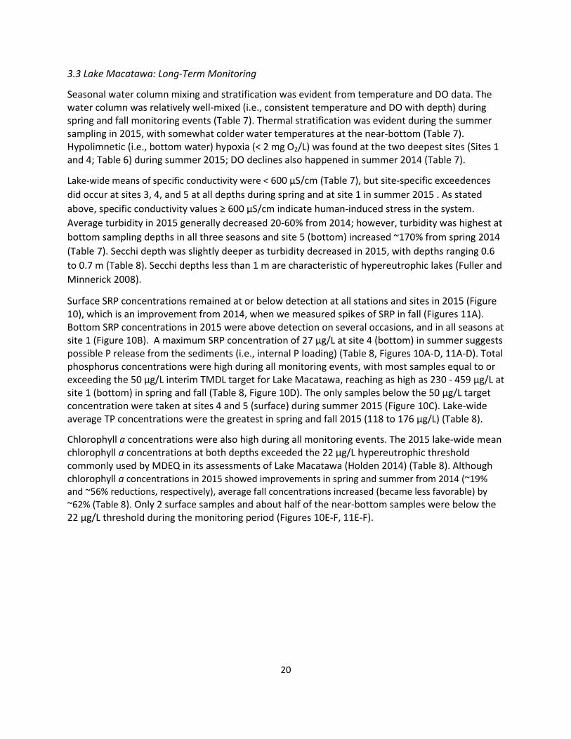
3.3 Lake Macatawa: Long-Term Monitoring

Seasonal water column mixing and stratification was evident from temperature and DO data. The water column was relatively well-mixed (i.e., consistent temperature and DO with depth) during spring and fall monitoring events (Table 7). Thermal stratification was evident during the summer sampling in 2015, with somewhat colder water temperatures at the near-bottom (Table 7). Hypolimnetic (i.e., bottom water) hypoxia (< 2 mg O2/L) was found at the two deepest sites (Sites 1 and 4; Table 6) during summer 2015; DO declines also happened in summer 2014 (Table 7).

Lake-wide means of specific conductivity were < 600 μS/cm (Table 7), but site-specific exceedences did occur at sites 3, 4, and 5 at all depths during spring and at site 1 in summer 2015 . As stated above, specific conductivity values ≥ 600 μS/cm indicate human-induced stress in the system. Average turbidity in 2015 generally decreased 20-60% from 2014; however, turbidity was highest at bottom sampling depths in all three seasons and site 5 (bottom) increased ~170% from spring 2014 (Table 7). Secchi depth was slightly deeper as turbidity decreased in 2015, with depths ranging 0.6 to 0.7 m (Table 8). Secchi depths less than 1 m are characteristic of hypereutrophic lakes (Fuller and Minnerick 2008).

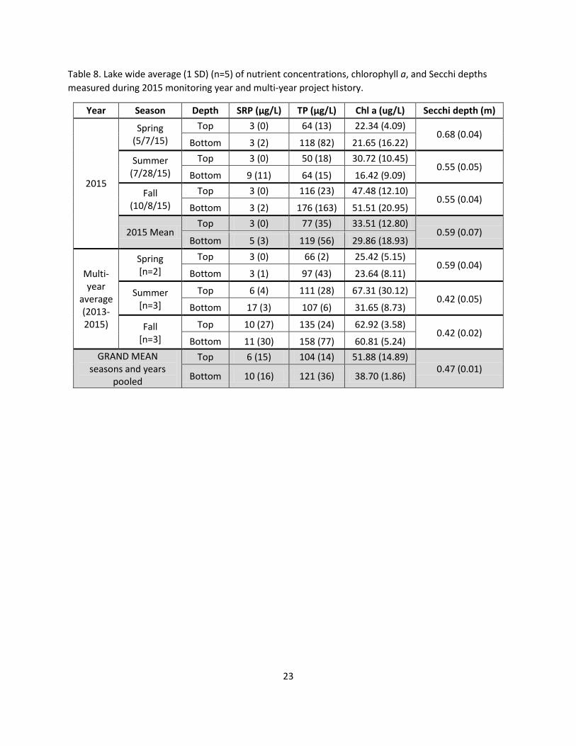
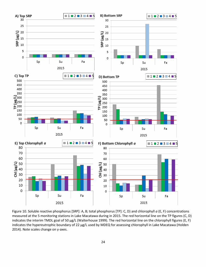
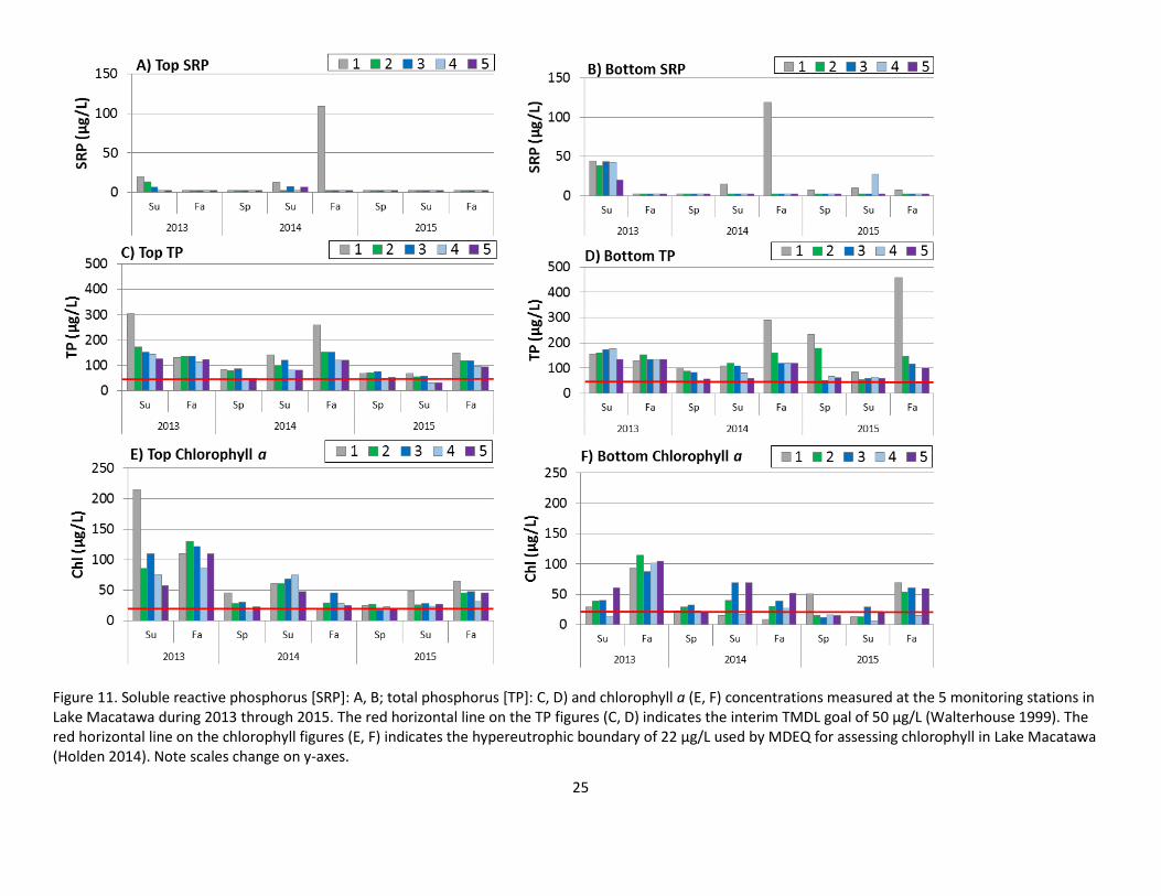
Surface SRP concentrations remained at or below detection at all stations and sites in 2015 (Figure 10), which is an improvement from 2014, when we measured spikes of SRP in fall (Figures 11A). Bottom SRP concentrations in 2015 were above detection on several occasions, and in all seasons at site 1 (Figure 10B). A maximum SRP concentration of 27 μg/L at site 4 (bottom) in summer suggests possible P release from the sediments (i.e., internal P loading) (Table 8, Figures 10A-D, 11A-D). Total phosphorus concentrations were high during all monitoring events, with most samples equal to or exceeding the 50 μg/L interim TMDL target for Lake Macatawa, reaching as high as 230 - 459 μg/L at site 1 (bottom) in spring and fall (Table 8, Figure 10D). The only samples below the 50 μg/L target concentration were taken at sites 4 and 5 (surface) during summer 2015 (Figure 10C). Lake-wide average TP concentrations were the greatest in spring and fall 2015 (118 to 176 μg/L) (Table 8).

Chlorophyll a concentrations were also high during all monitoring events. The 2015 lake-wide mean chlorophyll a concentrations at both depths exceeded the 22 μg/L hypereutrophic threshold commonly used by MDEQ in its assessments of Lake Macatawa (Holden 2014) (Table 8). Although chlorophyll a concentrations in 2015 showed improvements in spring and summer from 2014 (~19% and ~56% reductions, respectively), average fall concentrations increased (became less favorable) by ~62% (Table 8). Only 2 surface samples and about half of the near-bottom samples were below the 22 μg/L threshold during the monitoring period (Figures 10E-F, 11E-F).

21

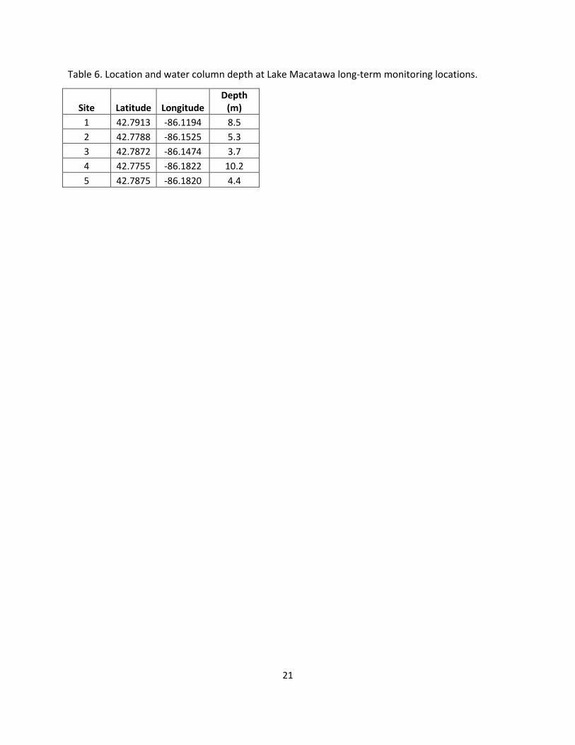
Table 6. Location and water column depth at Lake Macatawa long-term monitoring locations.

Site Latitude Longitude Depth

(m) 1 42.7913 -86.1194 8.5 2 42.7788 -86.1525 5.3 3 42.7872 -86.1474 3.7 4 42.7755 -86.1822 10.2 5 42.7875 -86.1820 4.4

22

Table 7. Lake-wide average (1 SD) (n=5) of select general water quality parameters recorded during 2015 monitoring year and multi-year project history.

Year Season Depth Temp. (C) DO (mg/L) SpCond (µS/cm) TDS (g/L) Turbidity (NTU)

2015

Spring (5/7/15)

Top 16.30 (1.45) 13.99 (0.77) 584 (77) 0.38 (0.05) 4.6 (1.0)

Mid 14.71 (1.35) 12.49 (1.80) 578 (75) 0.38 (0.05) 8.4 (3.1)

Bottom 13.99 (1.82) 12.09 (2.26) 541 (76) 0.35 (0.05) 14.1 (11.5)

Summer (7/28/15)

Top 26.43 (0.50) 12.18 (1.27) 524 (59) 0.34 (0.04) 9.0 (1.7)

Mid 24.49 (1.64) 7.79 (3.38) 486 (56) 0.32 (0.04) 9.2 (2.9)

Bottom 21.69 (2.81) 1.92 (1.47) 471 (44) 0.31 (0.03) 13.3 (4.4)

Fall (10/28/15)

Top 14.43 (0.63) 10.98 (0.71) 486 (46) 0.32 (0.03) 21.3 (2.7)

Mid 14.05 (0.92) 9.99 (0.40) 482 (50) 0.31 (0.03) 21.0 (3.2)

Bottom 13.39 (2.01) 8.25 (1.65) 482 (89) 0.31 (0.06) 27.7 (9.6)

2015 Mean

Top 19.05 (6.46) 12.38 (1.52) 531 (49) 0.35 (0.03) 11.6 (8.6)

Mid 17.75 (5.85) 10.09 (2.35) 515 (54) 0.33 (0.04) 12.9 (7.1)

Bottom 16.35 (4.63) 7.42 (5.14) 498 (38) 0.32 (0.02) 18.4 (8.1)

Multi-year

average ('13-'15)

Spring [n=2]

Top 14.42 (2.66) 12.83 (1.64) 594 (15) 0.39 (0.01) 9.0 (6.2)

Mid 13.48 (1.74) 12.00 (0.68) 594 (23) 0.39 (0.01) 11.4 (4.2)

Bottom 13.03 (1.35) 11.60 (0.70) 577 (51) 0.38 (0.03) 16.9 (3.9)

Summer [n=3]

Top 23.11 (2.88) 11.02 (1.05) 520 (44) 0.34 (0.03) 16.2 (6.6)

Mid 21.76 (2.39) 7.27 (1.41) 498 (45) 0.32 (0.03) 15.3 (5.4)

Bottom 19.17 (2.18) 2.51 (1.89) 447 (42) 0.29 (0.03) 22.1 (10.7)

Fall [n=3]

Top 14.66 (1.44) 10.03 (0.86) 502 (24) 0.33 (0.02) 25.5 (3.9)

Mid 14.50 (1.48) 9.42 (0.50) 502 (24) 0.33 (0.02) 26.2 (4.5)

Bottom 14.15 (1.62) 8.62 (0.34) 506 (28) 0.33 (0.02) 30.7 (2.8)

GRAND MEAN all sites, seasons, & years pooled

Top 17.40 (4.95) 11.29 (1.42) 539 (49) 0.35 (0.03) 16.9 (8.2) Mid 16.58 (4.52) 9.56 (2.37) 531 (54) 0.35 (0.04) 17.6 (7.7)

Bottom 15.45 (3.27) 7.57 (4.63) 510 (65) 0.33 (0.04) 23.2 (7.0)

23

Table 8. Lake wide average (1 SD) (n=5) of nutrient concentrations, chlorophyll a, and Secchi depths measured during 2015 monitoring year and multi-year project history.

Year Season Depth SRP (μg/L) TP (μg/L) Chl a (ug/L) Secchi depth (m)

2015

Spring (5/7/15)

Top 3 (0) 64 (13) 22.34 (4.09) 0.68 (0.04)

Bottom 3 (2) 118 (82) 21.65 (16.22)

Summer (7/28/15)

Top 3 (0) 50 (18) 30.72 (10.45) 0.55 (0.05)

Bottom 9 (11) 64 (15) 16.42 (9.09)

Fall (10/8/15)

Top 3 (0) 116 (23) 47.48 (12.10) 0.55 (0.04)

Bottom 3 (2) 176 (163) 51.51 (20.95)

2015 Mean Top 3 (0) 77 (35) 33.51 (12.80)

0.59 (0.07) Bottom 5 (3) 119 (56) 29.86 (18.93)

Multi-year

average (2013-2015)

Spring [n=2]

Top 3 (0) 66 (2) 25.42 (5.15) 0.59 (0.04)

Bottom 3 (1) 97 (43) 23.64 (8.11)

Summer [n=3]

Top 6 (4) 111 (28) 67.31 (30.12) 0.42 (0.05)

Bottom 17 (3) 107 (6) 31.65 (8.73)

Fall [n=3]

Top 10 (27) 135 (24) 62.92 (3.58) 0.42 (0.02)

Bottom 11 (30) 158 (77) 60.81 (5.24) GRAND MEAN

seasons and years pooled

Top 6 (15) 104 (14) 51.88 (14.89) 0.47 (0.01)

Bottom 10 (16) 121 (36) 38.70 (1.86)

24

Figure 10. Soluble reactive phosphorus [SRP]: A, B; total phosphorus [TP]: C, D) and chlorophyll a (E, F) concentrations measured at the 5 monitoring stations in Lake Macatawa during in 2015. The red horizontal line on the TP figures (C, D) indicates the interim TMDL goal of 50 μg/L (Walterhouse 1999). The red horizontal line on the chlorophyll figures (E, F) indicates the hypereutrophic boundary of 22 μg/L used by MDEQ for assessing chlorophyll in Lake Macatawa (Holden 2014). Note scales change on y-axes.

25

Figure 11. Soluble reactive phosphorus [SRP]: A, B; total phosphorus [TP]: C, D) and chlorophyll a (E, F) concentrations measured at the 5 monitoring stations in Lake Macatawa during 2013 through 2015. The red horizontal line on the TP figures (C, D) indicates the interim TMDL goal of 50 μg/L (Walterhouse 1999). The red horizontal line on the chlorophyll figures (E, F) indicates the hypereutrophic boundary of 22 μg/L used by MDEQ for assessing chlorophyll in Lake Macatawa (Holden 2014). Note scales change on y-axes.

26

4. Additional Studies

AWRI also is engaged in a number of research projects to help inform management decisions for Project Clarity. Below is a brief summary of those projects.

4.1 Tile Drains as a Source of Phosphorus:

This study is being conducted by Delilah Clement as part of her Masters of Science degree at AWRI. The work is focused on phosphorus (P) coming from tile drains, which in addition to surface runoff, can be an important P source, especially in agriculturally-dominated areas such as the Macatawa watershed. Delilah has been sampling tile drain effluent monthly 1) to measure total phosphorus (TP) and soluble reactive phosphorus (SRP; bioavailable form of P) concentrations and 2) conduct seasonal bioassays to determine the effect of tile drain P on algal growth and community structure. During March - December 2015, tile drain TP concentrations ranged from 10-560 µg/L and soluble reactive phosphorus (SRP) ranged from 5-447 µg/L. Four of six bioassays resulted in a positive relationship between SRP and algal growth, but results from only one bioassay were statistically significant. There was a clear change in the algal community structure when incubated in tile drain water, but dominance was by diatoms, not cyanobacteria as expected. Tile drain sampling will end in February 2016, with Delilah planning to defend in April 2016.

4.2 Two-Stage Ditches as Phosphorus Retention Devices

This study is being conducted by Emily Kindervater as part of her Masters of Science degree at AWRI. Emily is examining the mechanisms by which two-stage ditches retain P in their system. Emily is just beginning this research, but it will involve a survey of P fractions in the stream and bench sediment at two 2-stage ditches to assess where and how the P is being retained. This work will be completed in 2017.

4.3 Using High-Resolution Terrestrial LIDAR to Measure Bank Erosion in Lake Macatawa Watershed

AWRI researchers recently completed the second of three scheduled terrestrial LIDAR (Laser Imaging, Detection And Ranging) scans in December (Spring 2015; Late Fall 2015; Spring 2016) within three sub-catchments of the Lake Macatawa watershed. Researchers will use these LIDAR scans to accurately determine and quantify bank erosion rates occurring over the course of time at these specific sites. The high-resolution LIDAR scans capture the current physical condition of these targeted eroding stream banks (both an upstream and downstream location at each site) by transmitting and then recording high intensity laser light that is reflected back from the surface of the bank slope. These recorded scans are digital three dimensional representations of the stream bank down to the one millimeter scale, which can then be physically compared to future scans of these same sites to mathematically derive the amount of sediment lost or gained along the bank’s surface. The final LIDAR scans of the project are expected to be taken sometime in April, 2016.

5. Summary

The results of the 2015 monitoring effort were consistent with prior findings for Lake Macatawa and its watershed, confirming that water quality is severely impaired in this system (Holden 2014; Ogdahl et al. 2015). MDEQ has reported a strong positive relationship between flow and TP

27

concentrations in Macatawa watershed tributaries, with even minimal increases in flow resulting in substantial increases in TP concentration (Holden 2014). Tributary monitoring at the wetland restoration sites demonstrated the relationship between flow and degraded water quality, with storm events resulting in reduced dissolved oxygen, increased water temperature and nutrient concentrations, and very high turbidity. With TP concentrations climbing over 1,000 μg/L in the Macatawa River during storms, it is clear that the watershed can have a profound influence on Lake Macatawa during these episodic events. Indeed, modeled relationships by MDEQ revealed that flows > 100 cfs can cause TP concentrations to exceed 300 μg/L in Lake Macatawa (Holden 2014). High SRP concentrations in the Macatawa River during storms mean that a considerable fraction of the P entering Lake Macatawa is bioavailable and can be rapidly taken up by algae, potentially resulting in algal blooms. In addition to these immediate run-off impacts, it is likely that the excess P is being retained in the watershed, serving as legacy phosphorus, which can continue to serve as a P source for years and decades to come (Sharpley et al. 2013). Hence, it will take years of dedicated effort to manage and control this problem.

Degraded baseflow conditions reflect the chronic human-induced stress that the system is experiencing. Nutrient concentrations and specific conductance were both consistently high during baseflow, with TP averaging more than 100 μg/L in the Macatawa River. Nitrogen was perhaps an even greater concern during baseflow, with extremely high concentrations originating in the Peter’s Creek sub-basin, and leading to high concentrations in the Macatawa River downstream of the confluence. Although nutrient reduction efforts are focused on phosphorus, there is evidence for co-limitation of algal growth by both nitrogen and phosphorus in Lake Macatawa during summer and fall (Holden 2014; Abdimalik unpubl. data). Co-limitation of algae by nitrogen and phosphorus is gaining greater recognition in water bodies throughout the world (Conley et al. 2009). Thus, the high nitrogen concentrations in Peter’s Creek warrant future monitoring and consideration. There were no other site-specific trends observed in the tributary data that may influence future restoration evaluation.

MDEQ has been monitoring Lake Macatawa regularly (every 1-2 years) since 1996 to assess progress toward achieving the phosphorus TMDL target. They have consistently documented hypereutrophic conditions, including excessively high TP and chlorophyll concentrations, low DO, high turbidity, and shallow Secchi depths (Holden 2014). AWRI’s long-term monitoring results from 2013 to 2015 support MDEQ’s findings. As noted also by MDEQ, the eastern basin (i.e., site 1) is more highly degraded than the rest of the lake, reflecting the localized negative impact of the Macatawa River (Holden 2014). The periodic increased P concentrations in near-bottom samples suggest intermittent internal P loading from the sediments. However, given the excessive P loads entering the lake from Lake Macatawa, the external loads of P need to be controlled prior to a more detailed investigation of internal loading in Lake Macatawa and possible in-lake P mitigation.

These pre-restoration baseline conditions underscore the dire need for remediation in the Macatawa watershed. The magnitude of nutrient reduction that is necessary to satisfy the phosphorus TMDL and result in a healthy Lake Macatawa will require long-term and sustainable dedication, coordination, and cooperation among stakeholders and professionals. The successful execution of Project Clarity is a major step toward realizing the goals for Lake Macatawa. Continued monitoring as part of the project will document progress along the way.

28

5. Acknowledgements

Funding was provided through Project Clarity funds; our thanks to Travis Williams and Dan Callam of ODC for all of their help and knowledge of the area. We gratefully acknowledge the field and lab support provided by Mary Ogdahl, James Smit, Delilah Clement, Emily Kindervater, Travis Williams, Dan Callam, and Ben Heerspink. Brian Scull preformed P and N analysis in the laboratory.

6. References

APHA. 1992. Standard Methods for Examination of Water and Wastewater. 18th Edition. American Public Health Association.

Bhagat, Y. and C.R. Ruetz III. 2011. Temporal and fine-scale spatial variation in fish assemblage structure in a drowned river mouth system of Lake Michigan. Transactions of the American Fisheries Society 140: 1429-1440.

Cech, T.V. 2003. Principles of water resources. Wiley, New York, NY.

Chu, X. and A.D. Steinman. 2009. Combined event and continuous hydrologic modeling with HEC-HMS. ASCE Journal of Irrigation and Drainage Engineering 135: 119-124.

Conley, D.J., H.W. Paerl, R.W. Howarth, D.F. Boesch, S.P. Seitzinger, K.E. Havens, C. Lancelot, and G.E. Likens. 2009. Controlling eutrophication: nitrogen and phosphorus. Science 323: 1014-1015.Fuller, L.M. and R.J. Minnerick. 2008. State and Regional Water-Quality Characteristics and Trophic Conditions of Michigan’s Inland Lakes, 2001-2005: U.S. Geological Survey Scientific Investigations Report 2008-5188, 58p.

Holden, S. 2014. Monthly water quality assessment of Lake Macatawa and its tributaries, April-September 2012. Michigan Department of Environmental Quality, Water Resources Division. MI/DEQ/WRD-14/005

MWP (Macatawa Watershed Project). 2012. Macatawa Watershed Management Plan. Macatawa Area Coordinating Council, Holland, Michigan.

Ogdahl, M, M. Weinert, and A.D. Steinman. 2015. Project Clarity: 2014 Annual Monitoring Report. Available at: http://www.gvsu.edu/cms4/asset/DFC9A03B-95B4-19D5-F96AB46C60F3F345/2014_project_clarity_yearly_report_final.pdf

Sharpley, A., H.P. Jarvie, A. Buda, L. May, B. Spears, & P. Kleinman. 2013. Phosphorus legacy: Overcoming the effects of past management practices to mitigate future water quality impairment. Journal of Environmental Quality 42: 1308-1326.

Steinman, A.D., M. Ogdahl, R. Rediske, C.R. Ruetz III, B.A. Biddanda, and L. Nemeth. 2008. Current status and trends in Muskegon Lake, Michigan. Journal of Great Lakes Research 34: 169-188.

Steinman, A.D., M.E. Ogdahl, and C.R. Ruetz III. 2011. An environmental assessment of a small, shallow lake threatened by urbanization. Environmental Monitoring and Assessment 173: 193-209

U.S. EPA. 1993. Methods for Chemical Analysis of Inorganic Substances in Environmental Samples. EPA-600/4-79R-93-020/100.

http://www.gvsu.edu/cms4/asset/DFC9A03B-95B4-19D5-F96AB46C60F3F345/2014_project_clarity_yearly_report_final.pdf

http://www.gvsu.edu/cms4/asset/DFC9A03B-95B4-19D5-F96AB46C60F3F345/2014_project_clarity_yearly_report_final.pdf

29

Walterhouse, M. 1999. Total Maximum Daily Load for Phosphorus in Lake Macatawa, January 20, 1999. MDEQ Submittal to U.S. Environmental Protection Agency.

1

Long-Term Fish Monitoring of Lake Macatawa: Results from Year 2

Carl R. Ruetz III1 and Andrya Whitten Annis Water Resources Institute Grand Valley State University

740 W. Shoreline Drive, Muskegon, Michigan 49441

12 January 2016

An Annual Report to the

Outdoor Discovery Center Holland, Michigan 49423

1 Corresponding author; Office: 616-331-3946; E-mail: [email protected]

2

Introduction

This study was initiated to provide critical information on littoral fish populations that

will be used to evaluate the performance of watershed restoration activities that are part of

Project Clarity. Although we do not expect the benefits of the restoration activities in the

watershed to be expressed in Lake Macatawa immediately, establishing baseline conditions in

Lake Macatawa will be critical for evaluating ecological change over time. In autumn 2014, we

initiated a long-term monitoring effort of the littoral fish assemblage of Lake Macatawa. Our

fish sampling plan for Lake Macatawa is similar to our ongoing, long-term (since 2003)

monitoring effort in Muskegon Lake (Bhagat and Ruetz 2011). By using the same monitoring

protocols in each water body, Muskegon Lake can serve as a “control” to evaluate temporal

changes in Lake Macatawa in an effort to assess how the lake is responding to watershed

restoration activities. Our primary objective in the second year of sampling was to continue to

characterize the pre-restoration (baseline) littoral fish assemblage. We made preliminary

comparisons with our ongoing work in Muskegon Lake (see Ruetz et al. 2007; Bhagat and Ruetz

2011) as well as with six Lake Michigan drowned river mouths for which we have data (see

Janetski and Ruetz 2015). However, the true value of this fish monitoring effort will come in

future years as we examine how the littoral fish assemblage responds to restoration activities in

the watershed.

Methods

Study sites.—Lake Macatawa is a drowned river mouth lake in Holland, Michigan that is

located on the eastern shore of Lake Michigan in Ottawa County. Lake Macatawa has an area of

7.20 km2, mean depth of 3.66 m, and maximum depth of 12.19 m (MDNR 2011). The shoreline

has high residential and commercial development, and the watershed consists mainly of

3

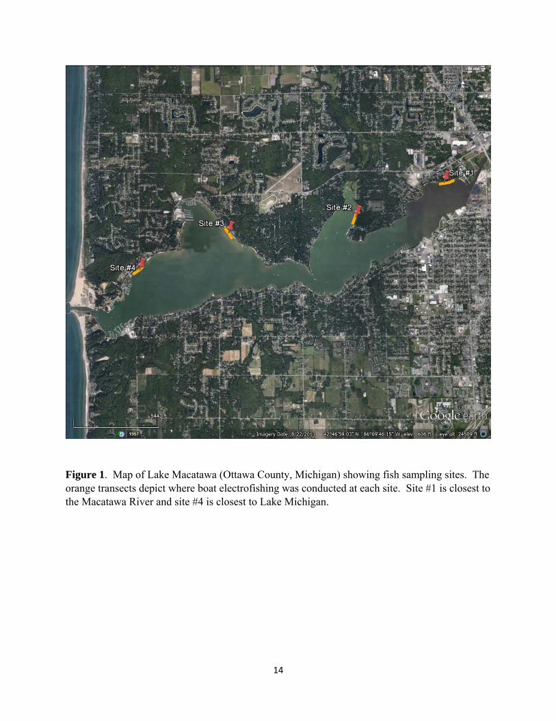
agricultural land (MDNR 2011). Fish sampling was conducted at four littoral sites in Lake

Macatawa that represented a gradient from the mouth of the Macatawa River to the connecting

channel with Lake Michigan (Figure 1; Table 1).

Fish sampling.—At each study site, we sampled fish via fyke netting and boat

electrofishing. Fyke nets were set on 8 September 2015 during daylight hours (i.e., between

1030 and 1430) and fished for about 24.8 h (range = 24.5-24.9 h). Three fyke nets (4-mm mesh)

were fished at each site; two fyke nets were set facing each other and parallel to the shoreline,

whereas a third fyke net was set perpendicular to the shoreline following the protocol used by

Bhagat and Ruetz (2011). A description of the design of the fyke nets is reported in Breen and

Ruetz (2006). We conducted nighttime boat electrofishing at each site on 10 September 2015. A

10-min (pedal time) electrofishing transect was conducted parallel to the shoreline at each site

with two people at the front of the boat to net fish. The electrofishing boat was equipped with a

Smith-Root 5.0 generator-powered pulsator control box (pulsed DC, 220 volts, ~7 amp). For

both sampling methods, all fish captured were identified to species, measured (total length), and

released in the field; however, some specimens were preserved to confirm identifications in the

laboratory. We also measured water quality variables (i.e., temperature, dissolved oxygen,

specific conductivity, total dissolved solids, turbidity, pH, oxidation-reduction potential, and

chlorophyll a) in the middle of the water column using a YSI 6600 multi-parameter data sonde.

We made one measurement at each fyke net (n = 12) and one measurement at the beginning of

each electrofishing transect (n = 4). We measured the water depth at the mouth of each fyke net

and visually estimated the percent macrophyte cover for the length of the lead between the wings

of each fyke net (see Bhagat and Ruetz 2011). We also visually estimated the percent

macrophyte cover for the length of each electrofishing transect during fish sampling.

4

Results and Discussion

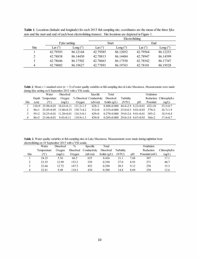
We characterized water quality variables at each site during fish sampling (Tables 2 & 3).

The mean water depth at fyke nets was 96 cm (Table 2). Water temperature was slightly (~1.5

°C) warmer when we conducted fyke netting compared with boat electrofishing (Tables 2 & 3).

We visually observed few aquatic macrophytes during fish sampling. During fyke netting, mean

% cover of macrophytes was zero at site #1 and <10% at the remaining sites (site #2: 5%; site

#3: 6%; site #4: 3%). During electrofishing transects, we visually estimated macrophyte cover to

be ≤25% at all sites (site #1: 0%; site #2: 10%; site #3: 10%; site #4: 25%), which was greater

than our estimates during fyke netting (note that visual estimates of % macrophyte cover for

electrofishing is over a greater area at each site than fyke netting). The low densities of

macrophytes in Lake Macatawa is presumably because of insufficient light penetrating the water

column to allow the submersed plants to grow; both turbidity from inflowing sediment and

abundant phytoplankton growth in the lake water column can reduce light penetration. Given the

importance of aquatic macrophytes as habitat for fish (e.g., Radomski and Goeman 2001), their

return is an important goal for the restoration of natural fish communities in Lake Macatawa.

Compared to six Lake Michigan drowned river mouths, water quality in Lake Macatawa

was most similar to Kalamazoo Lake, especially with respect to high turbidity and specific

conductivity (Janetski and Ruetz 2015). Turbidity and specific conductivity were higher in Lake

Macatawa than Muskegon Lake, the drowned river mouth lake that we have the longest time

series of water quality observations (Bhagat and Ruetz 2011). High levels of turbidity and

specific conductivity often are associated with relatively high anthropogenic disturbance in Great

Lakes coastal wetlands (Uzarski et al. 2005). Thus, the water quality we measured in Lake

Macatawa appears on the degraded side of the spectrum among Lake Michigan drowned river

mouths (see Uzarski et al. 2005, Janetski and Ruetz 2015).

5

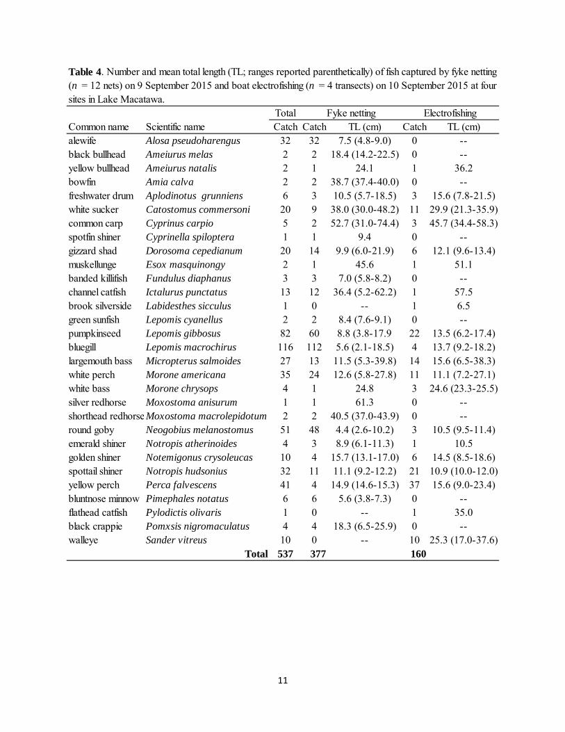
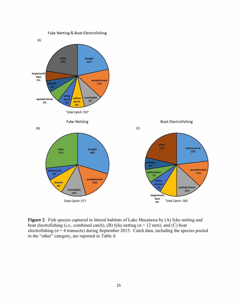
We captured 537 fish comprising 30 species in Lake Macatawa (Table 4). The most

abundant fishes in the combined catch of both gears (fyke netting and boat electrofishing) were

bluegill (22%), pumpkinseed (15%), round goby (9%), yellow perch (8%), white perch (7%),

alewife (6%), spottail shiner (6%), and largemouth bass (5%), which composed 77% of the total

catch (Figure 2A). Three of the 30 species captured were non-native to the Great Lakes basin

(Bailey et al. 2004)—alewife (6%), white perch (7%), and round goby (9%)—which composed

22% of the total catch (Table 4). Although not an abundant species in our catch, we captured

muskellunge—a native predator (Becker 1983)—for the first time (during this study) in Lake

Macatawa (Table 4). The Michigan Department of Natural Resources has stocked muskellunge

in Lake Macatawa annually since 2012 (MDNR 2016).

We captured more than twice as many fish in fyke netting than boat electrofishing (Table

4). Similarly, more fish species were captured in fyke netting (27 species) than boat

electrofishing (20 species). Ten fish species were collected only by fyke netting, and three

species were collected only by boat electrofishing. Thus, using both sampling gears provided a

better characterization of the littoral fish assemblage of Lake Macatawa than either gear by itself.

This finding was consistent with research in Muskegon Lake that found a similar pattern where

small-bodied fishes were better represented in fyke netting and large-bodied fishes were better

represented in nighttime boat electrofishing (Ruetz et al. 2007).

In fyke netting, bluegill (30%), pumpkinseed (16%), round goby (13%), alewife (8%),

and white perch (6%) were the most abundant fishes captured, which composed 73% of the total

fish captured (Figure 2B). Although bluegill was the most abundant species in the catch at sites

#1 and #2, alewife was most common at site #3 and pumpkinseed was most common at site #4

(Table 5). The next most abundant species in the catch at sites #1 and #4 was the round goby

(Table 5), whereas there was not one species that was clearly next most abundant in the catch at

6

sites #2 and #3. Largemouth bass and gizzard shad were nearly equally represented in the catch

as the next most abundant species at site #2, and pumpkinseed, bluegill, white perch, and spottail

shiner were equally represented in the catch as the next most abundant species at site #3 (Table

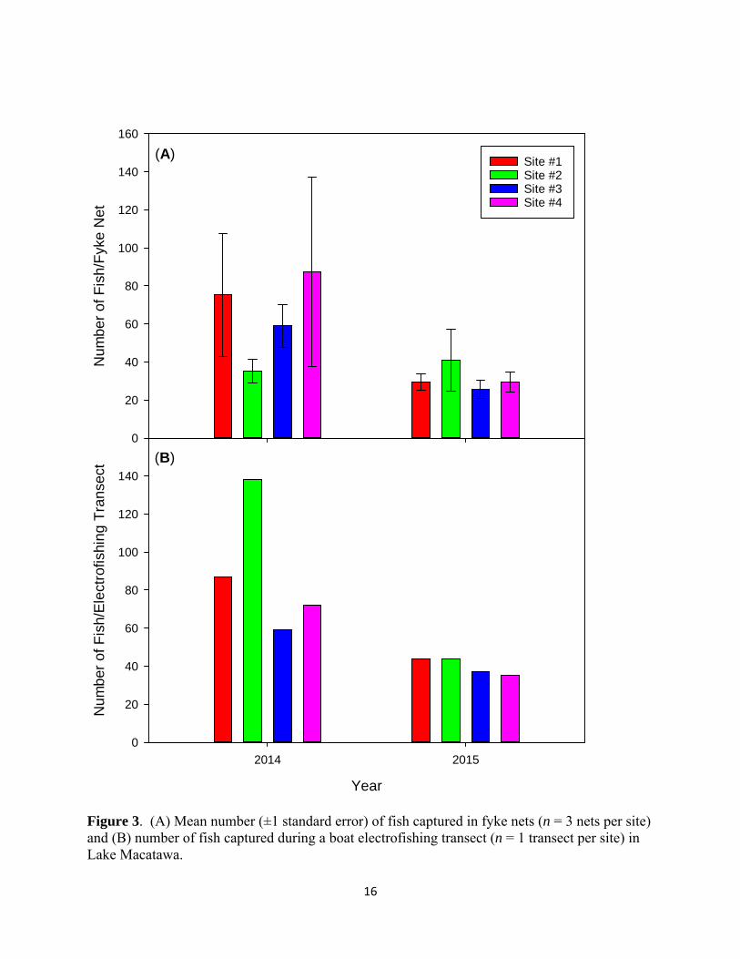
5). There also was variation in total catch among the sites, with site #2 having the highest catch

and site #3 having the lowest catch, although the variation in total catch among sites #1, #3, and

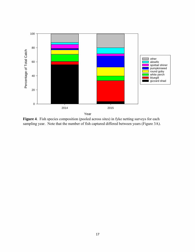
#4 was small (Table 5; Figure 3A). Compared with 2014 fyke netting surveys, the most

abundant species in the catch varied between years (Figure 4) as did the patterns in total catch

among sites (Figure 3A). However, as we continue our monitoring of Lake Macatawa, we will

be better able to assess whether these spatial patterns among sites are stable or dynamic over

time.

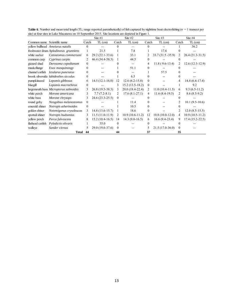
In boat electrofishing, the most abundant fishes captured were yellow perch (23%),

pumpkinseed (14%), spottail shiner (13%), largemouth bass (9%), white sucker (7%), white

perch (7%), and walleye (6%), which composed 79% of the total catch (Figure 2C). The fish

assemblage was not dominated by a single fish species at every site in the electrofishing catch,

which contrasted with what was observed in fyke netting. Yellow perch was among the most

abundant species in the catch at sites #1, #2, and #4, whereas spottail shiner was most abundant

at site #3 (Table 6). Unlike fyke netting, total catch was similar among sites in 2015 (Figure

3B). Thus, there was not a strong, positive association in total catch across sites between the two

sampling gears (Tables 5 & 6). Compared with 2014 boat electrofishing surveys, the most

abundant species in the catch varied between years (Figure 5), although the pattern was weaker

than what was observed for fyke netting (Figure 4), and total catch was lower in 2015 (Figure

3B).

In conclusion, the observations reported here provide the second year of a 5 year effort to

characterize the littoral fish assemblage of Lake Macatawa. This monitoring effort will provide

7

a baseline to assess how the fish assemblage responds to restoration activities in the Lake

Macatawa watershed. Although we only have completed two years of fish monitoring, we

observed differences in total catch (Figure 3) and fish species composition of the catch between

2014 and 2015 (Figures 4 & 5) even though we observed similar water quality (i.e., high specific

conductivity and turbidity; Figure 6) and habitat (i.e., low densities of submersed macrophytes)

during both years. With respect to the catch, we captured fewer fish in both sampling gears at

almost every site in 2015 compared with 2014 (Figure 3). Although gizzard shad and white bass

dominated fyke netting catch in 2014, bluegill and pumpkinseed were dominant in 2015 (Figure

4). There was less variability in the fish species composition of boat electrofishing surveys

compared with fyke netting surveys (Figures 4 & 5). Nevertheless, not too much weight should

be attributed to differences between only two sampling years. Once we accumulate several years

of observations, we will be able to make more robust inferences about the littoral fish

assemblage of Lake Macatawa (both in terms of assessing the baseline and change over time) as

well as how the assemblage compares with other drowned river mouth lakes in the region.

Acknowledgements

We thank Dr. Alan Steinman for facilitating our role in fish monitoring as part of Project

Clarity as well as comments on this report. Brandon Harris provided assistance with fish

sampling. Maggie Weinert was instrumental in coordinating logistics, site selection, and field

work.

8

References

Bailey, R.M., W.C. Latta, and G.R. Smith. 2004. An atlas of Michigan fishes with keys and

illustrations for their identification. Miscellaneous Publications, Museum of Zoology,

University of Michigan, No. 192.

Becker, G.C. 1983. Fishes of Wisconsin. University of Wisconsin Press, Madison.

Bhagat, Y., and C.R. Ruetz III. 2011. Temporal and fine-scale spatial variation in fish

assemblage structure in a drowned river mouth system of Lake Michigan. Transactions

of the American Fisheries Society 140:1429-1440.

Breen, M.J., and C.R. Ruetz III. 2006. Gear bias in fyke netting: evaluating soak time, fish

density, and predators. North American Journal of Fisheries Management 26:32-41.

Janetski, D.J., and C.R. Ruetz III. 2015. Spatiotemporal patterns of fish community

composition in Great Lakes drowned river mouths. Ecology of Freshwater Fish 24:493-

504.

Michigan Department of Natural Resources (MDNR). 2011. Lake Macatawa Ottawa County.

Fish Collection System (printed 6/11/2011). Accessed at http://www.the-macc.org/wp-

content/uploads/History-of-Lake-Mactawa-and-Fish.pdf (on 12/1/2014).

Michigan Department of Natural Resources (MDNR). 2016. Fish Stocking Database

(http://www.michigandnr.com/fishstock/). Accessed on 8 January 2016.

Radomski, P., and T.J. Goeman. 2001. Consequences of human lakeshore development on

emergent and floating-leaf vegetation abundance. North American Journal of Fisheries

Management 21:46-61.

Ruetz, C.R., III, D.G. Uzarski, D.M. Krueger, and E.S. Rutherford. 2007. Sampling a littoral

fish assemblage: comparing small-mesh fyke netting and boat electrofishing. North

American Journal of Fisheries Management 27:825-831.

9

Uzarski, D.G., T.M. Burton, M.J. Cooper, J.W. Ingram, and S.T.A. Timmermans. 2005. Fish

habitat use within and across wetland classes in coastal wetlands of the five Great Lakes:

development of a fish-based index of biotic integrity. Journal of Great Lakes Research

31(Suppl. 1):171-187.

10

Site Lat (°) Long (°) Lat (°) Long (°) Lat (°) Long (°)1 42.79593 86.12144 42.79585 86.12052 42.79564 86.122532 42.78838 86.14430 42.78813 86.14484 42.78947 86.143993 42.78646 86.17502 42.78663 86.17550 42.78542 86.173474 42.78002 86.19627 42.77891 86.19763 42.78101 86.19528

Table 1. Locations (latitude and longitude) for each 2015 fish sampling site; coordinates are the mean of the three fyke nets and the start and end of each boat electrofishing transect. Site locations are depicted in Figure 1.

Electrofishing Fyke netting Start End

DepthSite (cm) pH

1 110±9 25.98±0.03 10.63±0.11 131.2±1.5 628±1 0.408±0.000 44.4±2.9 8.23±0.01 432±10 53.5±0.72 96±1 25.45±0.05 13.00±0.33 158.7±4.2 512±0 0.333±0.000 25.8±0.3 9.01±0.03 379±2 36.7±1.93 95±2 24.25±0.01 11.20±0.01 134.3±0.1 429±0 0.279±0.000 39.0±2.6 9.01±0.01 385±2 18.5±0.44 86±5 23.44±0.01 9.43±0.11 110.9±1.3 439±0 0.285±0.000 29.8±3.0 8.67±0.03 366±2 17.4±0.7

Turbidity (NTU)

Oxidation Reduction Potential

Chlorophyll a (ug/L)

Table 2. Mean ± 1 standard error (n = 3) of water quality variables at fish sampling sites in Lake Macatawa. Measurements were made during fyke netting on 8 September 2015 with a YSI sonde.

Water Temperature

(°C)

Dissolved Oxygen (mg/L)

% Dissolved Oxygen

Specific Conductivity

(uS/cm)

Total Dissolved

Solids (g/L)

Site pH1 24.25 5.56 66.5 655 0.426 21.1 7.68 307 17.12 23.55 12.99 153.2 539 0.350 27.0 8.93 271 40.73 22.66 12.72 147.5 452 0.294 20.5 9.12 258 15.34 22.81 9.48 110.3 430 0.280 14.8 8.69 258 12.6

Turbidity (NTU)

Oxidation Reduction

Potential (mV)Chlorophyll a

(ug/L)

Table 3. Water quality variables at fish sampling sites in Lake Macatawa. Measurements were made during nighttime boat electrofishing on 10 September 2015 with a YSI sonde.

Water Temperature

(°C)

% Dissolved Oxygen

Dissolved Oxygen (mg/L)

Specific Conductivity

(uS/cm)

Total Dissolved

Solids (g/L)

11

TotalCommon name Scientific name Catch Catch TL (cm) Catch TL (cm)alewife Alosa pseudoharengus 32 32 7.5 (4.8-9.0) 0 --black bullhead Ameiurus melas 2 2 18.4 (14.2-22.5) 0 --yellow bullhead Ameiurus natalis 2 1 24.1 1 36.2bowfin Amia calva 2 2 38.7 (37.4-40.0) 0 --freshwater drum Aplodinotus grunniens 6 3 10.5 (5.7-18.5) 3 15.6 (7.8-21.5)white sucker Catostomus commersoni 20 9 38.0 (30.0-48.2) 11 29.9 (21.3-35.9)common carp Cyprinus carpio 5 2 52.7 (31.0-74.4) 3 45.7 (34.4-58.3)spotfin shiner Cyprinella spiloptera 1 1 9.4 0 --gizzard shad Dorosoma cepedianum 20 14 9.9 (6.0-21.9) 6 12.1 (9.6-13.4)muskellunge Esox masquinongy 2 1 45.6 1 51.1banded killifish Fundulus diaphanus 3 3 7.0 (5.8-8.2) 0 --channel catfish Ictalurus punctatus 13 12 36.4 (5.2-62.2) 1 57.5brook silverside Labidesthes sicculus 1 0 -- 1 6.5green sunfish Lepomis cyanellus 2 2 8.4 (7.6-9.1) 0 --pumpkinseed Lepomis gibbosus 82 60 8.8 (3.8-17.9 22 13.5 (6.2-17.4)bluegill Lepomis macrochirus 116 112 5.6 (2.1-18.5) 4 13.7 (9.2-18.2)largemouth bass Micropterus salmoides 27 13 11.5 (5.3-39.8) 14 15.6 (6.5-38.3)white perch Morone americana 35 24 12.6 (5.8-27.8) 11 11.1 (7.2-27.1)white bass Morone chrysops 4 1 24.8 3 24.6 (23.3-25.5)silver redhorse Moxostoma anisurum 1 1 61.3 0 --shorthead redhorseMoxostoma macrolepidotum 2 2 40.5 (37.0-43.9) 0 --round goby Neogobius melanostomus 51 48 4.4 (2.6-10.2) 3 10.5 (9.5-11.4)emerald shiner Notropis atherinoides 4 3 8.9 (6.1-11.3) 1 10.5golden shiner Notemigonus crysoleucas 10 4 15.7 (13.1-17.0) 6 14.5 (8.5-18.6)spottail shiner Notropis hudsonius 32 11 11.1 (9.2-12.2) 21 10.9 (10.0-12.0)yellow perch Perca falvescens 41 4 14.9 (14.6-15.3) 37 15.6 (9.0-23.4)bluntnose minnow Pimephales notatus 6 6 5.6 (3.8-7.3) 0 --flathead catfish Pylodictis olivaris 1 0 -- 1 35.0black crappie Pomxsis nigromaculatus 4 4 18.3 (6.5-25.9) 0 --walleye Sander vitreus 10 0 -- 10 25.3 (17.0-37.6)

Total 537 377 160

Fyke netting Electrofishing

Table 4. Number and mean total length (TL; ranges reported parenthetically) of fish captured by fyke netting (n = 12 nets) on 9 September 2015 and boat electrofishing (n = 4 transects) on 10 September 2015 at four sites in Lake Macatawa.

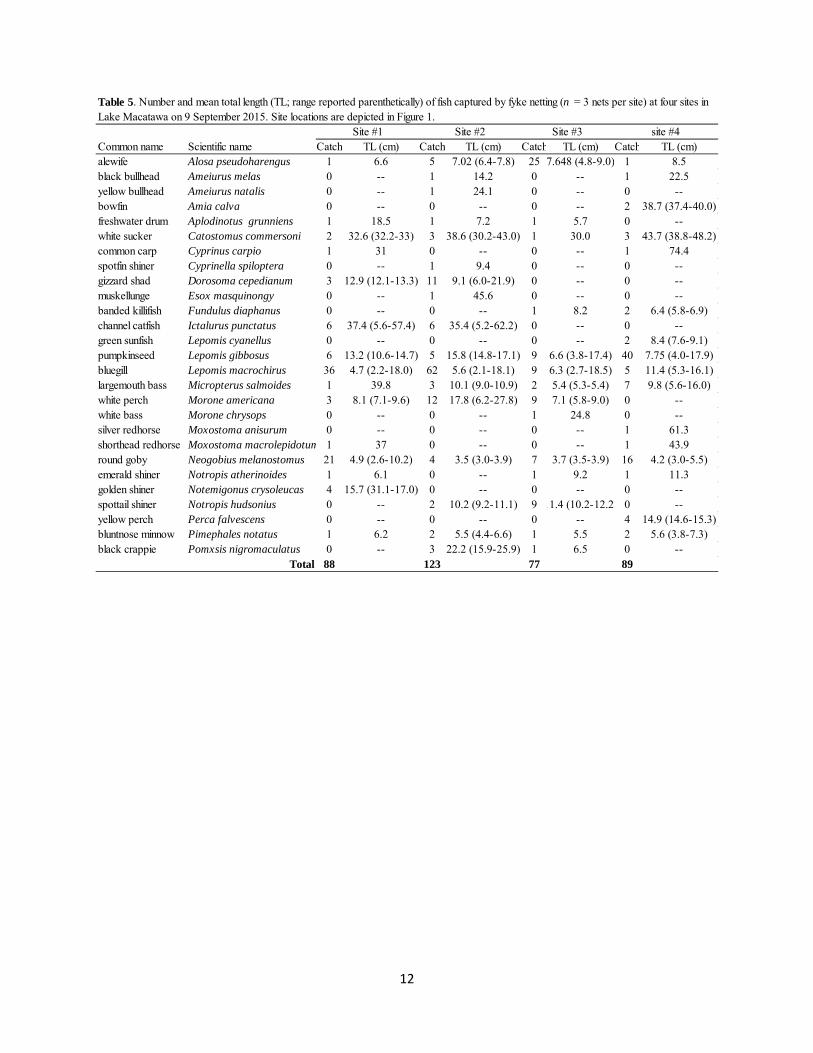
12

Common name Scientific name Catch TL (cm) Catch TL (cm) Catch TL (cm) Catch TL (cm)alewife Alosa pseudoharengus 1 6.6 5 7.02 (6.4-7.8) 25 7.648 (4.8-9.0) 1 8.5black bullhead Ameiurus melas 0 -- 1 14.2 0 -- 1 22.5yellow bullhead Ameiurus natalis 0 -- 1 24.1 0 -- 0 --bowfin Amia calva 0 -- 0 -- 0 -- 2 38.7 (37.4-40.0)freshwater drum Aplodinotus grunniens 1 18.5 1 7.2 1 5.7 0 --white sucker Catostomus commersoni 2 32.6 (32.2-33) 3 38.6 (30.2-43.0) 1 30.0 3 43.7 (38.8-48.2)common carp Cyprinus carpio 1 31 0 -- 0 -- 1 74.4spotfin shiner Cyprinella spiloptera 0 -- 1 9.4 0 -- 0 --gizzard shad Dorosoma cepedianum 3 12.9 (12.1-13.3) 11 9.1 (6.0-21.9) 0 -- 0 --muskellunge Esox masquinongy 0 -- 1 45.6 0 -- 0 --banded killifish Fundulus diaphanus 0 -- 0 -- 1 8.2 2 6.4 (5.8-6.9)channel catfish Ictalurus punctatus 6 37.4 (5.6-57.4) 6 35.4 (5.2-62.2) 0 -- 0 --green sunfish Lepomis cyanellus 0 -- 0 -- 0 -- 2 8.4 (7.6-9.1)pumpkinseed Lepomis gibbosus 6 13.2 (10.6-14.7) 5 15.8 (14.8-17.1) 9 6.6 (3.8-17.4) 40 7.75 (4.0-17.9)bluegill Lepomis macrochirus 36 4.7 (2.2-18.0) 62 5.6 (2.1-18.1) 9 6.3 (2.7-18.5) 5 11.4 (5.3-16.1)largemouth bass Micropterus salmoides 1 39.8 3 10.1 (9.0-10.9) 2 5.4 (5.3-5.4) 7 9.8 (5.6-16.0)white perch Morone americana 3 8.1 (7.1-9.6) 12 17.8 (6.2-27.8) 9 7.1 (5.8-9.0) 0 --white bass Morone chrysops 0 -- 0 -- 1 24.8 0 --silver redhorse Moxostoma anisurum 0 -- 0 -- 0 -- 1 61.3shorthead redhorse Moxostoma macrolepidotum 1 37 0 -- 0 -- 1 43.9round goby Neogobius melanostomus 21 4.9 (2.6-10.2) 4 3.5 (3.0-3.9) 7 3.7 (3.5-3.9) 16 4.2 (3.0-5.5)emerald shiner Notropis atherinoides 1 6.1 0 -- 1 9.2 1 11.3golden shiner Notemigonus crysoleucas 4 15.7 (31.1-17.0) 0 -- 0 -- 0 --spottail shiner Notropis hudsonius 0 -- 2 10.2 (9.2-11.1) 9 11.4 (10.2-12.2 0 --yellow perch Perca falvescens 0 -- 0 -- 0 -- 4 14.9 (14.6-15.3)bluntnose minnow Pimephales notatus 1 6.2 2 5.5 (4.4-6.6) 1 5.5 2 5.6 (3.8-7.3)black crappie Pomxsis nigromaculatus 0 -- 3 22.2 (15.9-25.9) 1 6.5 0 --

Total 88 123 77 89

Site #1 Site #2 Site #3 site #4

Table 5. Number and mean total length (TL; range reported parenthetically) of fish captured by fyke netting (n = 3 nets per site) at four sites in Lake Macatawa on 9 September 2015. Site locations are depicted in Figure 1.

13

Common name Scientific name Catch TL (cm) Catch TL (cm) Catch TL (cm) Catch TL (cm)yellow bullhead Ameiurus natalis 0 -- 0 -- 0 -- 1 36.2freshwater drum Aplodinotus grunniens 1 21.5 1 7.8 1 17.6 0 --white sucker Catostomus commersoni 6 29.2 (22.1-33.6) 1 33.1 2 33.7 (31.5 -35.9) 2 26.4 (21.3-31.5)common carp Cyprinus carpio 2 46.4 (34.4-58.3) 1 44.5 0 -- 0 --gizzard shad Dorosoma cepedianum 0 -- 0 -- 4 11.8 ( 9.6-13.4) 2 12.6 (12.3-12.9)muskellunge Esox masquinongy 0 -- 1 51.1 0 -- 0 --channel catfish Ictalurus punctatus 0 -- 0 -- 1 57.5 0 --brook silverside labidesthes sicculus 0 -- 1 6.5 0 -- 0 --pumpkinseed Lepomis gibbosus 6 14.5 (12.1-16.0) 12 12.6 (6.2-15.8) 0 -- 4 14.4 (6.4-17.4)bluegill Lepomis macrochirus 0 -- 3 15.2 (13.5-18.2) 0 -- 1 9.2largemouth bass Micropterus salmoides 3 26.8 (19.5-38.3) 3 20.0 (18.4-22.4) 2 11.0 (10.4-11.5) 6 9.3 (6.5-11.2)white perch Morone americana 3 7.7 (7.2-8.1) 2 17.6 (8.1-27.1) 4 11.6 (8.4-19.5) 2 8.6 (8.5-9.2)white bass Morone chrysops 3 24.6 (23.3-25.5) 0 -- 0 -- 0 --round goby Neogobius melanostomus 0 -- 1 11.4 0 -- 2 10.1 (9.5-10.6)emerald shiner Notropis atherinoides 0 -- 1 10.5 0 -- 0 --golden shiner Notemigonus crysoleucas 3 14.8 (13.6-15.7) 1 18.6 0 -- 2 12.0 (8.5-15.5)spottail shiner Notropis hudsonius 3 11.5 (11.0-11.9) 2 10.9 (10.6-11.2) 12 10.8 (10.0-12.0) 4 10.9 (10.5-11.2)yellow perch Perca falvescens 8 15.2 (10.4-16.5) 14 14.3 (9.0-16.5) 6 16.6 (9.4-23.4) 9 17.4 (15.2-22.5)flathead catfish Pylodictis olivaris 1 35.0 0 -- 0 -- 0 --walleye Sander vitreus 5 29.0 (19.6-37.6) 0 -- 5 21.5 (17.0-36.0) 0 --

Total 44 44 37 35

Site #1 Site #2 Site #3 Site #4

Table 6. Number and mean total length (TL; range reported parenthetically) of fish captured by nighttime boat electrofishing (n = 1 transect per site) at four sites in Lake Macatawa on 10 September 2015. Site locations are depicted in Figure 1.

14

Figure 1. Map of Lake Macatawa (Ottawa County, Michigan) showing fish sampling sites. The orange transects depict where boat electrofishing was conducted at each site. Site #1 is closest to the Macatawa River and site #4 is closest to Lake Michigan.

15

Figure 2. Fish species captured in littoral habitats of Lake Macatawa by (A) fyke netting and boat electrofishing (i.e., combined catch), (B) fyke netting (n = 12 nets), and (C) boat electrofishing (n = 4 transects) during September 2015. Catch data, including the species pooled in the “other” category, are reported in Table 4.

16

Figure 3. (A) Mean number (±1 standard error) of fish captured in fyke nets (n = 3 nets per site) and (B) number of fish captured during a boat electrofishing transect (n = 1 transect per site) in Lake Macatawa.

Num

ber o

f Fis

h/Fy

ke N

et

0

20

40

60

80

100

120

140

160


(A)

Year

2014 2015

Num

ber o

f Fis

h/El

ectro

fishi

ng T

rans

ect

0

20

40

60

80

100

120

140(B)

17

Figure 4. Fish species composition (pooled across sites) in fyke netting surveys for each sampling year. Note that the number of fish captured differed between years (Figure 3A).

Year

2014 2015

Perc

enta

ge o

f Tot

al C

atch

0

20

40

60

80

100

gizzard shad bluegill white perch round goby pumpkinseed spottail shiner alewife other

18

Figure 5. Fish species composition (pooled across sites) in boat electrofishing surveys for each sampling year. Note that the number of fish captured differed between years (Figure 3B).

Year

2014 2015

Perc

enta

ge o

f Tot

al C

atch

0

20

40

60

80

100

yellow perch white perch pumpkinseed spottail shiner largemouth bass walleye white sucker other

19

Figure 6. Mean (A) specific conductivity and (B) turbidity measured during fyke netting in Lake Macatawa. Error bars represent ±1 standard error (n = 3 nets per site), although they may to small to be visible for some means.

Spec

ific

Con

duct

ivity

(uS/

cm)

0

200

400

600

800


(A)

Year

2014 2015

Turb

idity

(NTU

)

0

10

20

30

40

50

(B)

project clarity 2015 annual monitoring report … project clarity 2015 annual monitoring report...

Documents