project portfolio evaluation and selection using
TRANSCRIPT
Purdue UniversityPurdue e-Pubs
Open Access Dissertations Theses and Dissertations
Fall 2014
Project portfolio evaluation and selection usingmathematical programming and optimizationmethodsHugo CaballeroPurdue University
Follow this and additional works at: https://docs.lib.purdue.edu/open_access_dissertations
Part of the Business Administration, Management, and Operations Commons
This document has been made available through Purdue e-Pubs, a service of the Purdue University Libraries. Please contact [email protected] foradditional information.
Recommended CitationCaballero, Hugo, "Project portfolio evaluation and selection using mathematical programming and optimization methods" (2014).Open Access Dissertations. 237.https://docs.lib.purdue.edu/open_access_dissertations/237

PURDUE UNIVERSITY GRADUATE SCHOOL
Thesis/Dissertation Acceptance
To the best of my knowledge and as understood by the student in the Thesis/Dissertation Agreement, Publication Delay, and Certification/Disclaimer (Graduate School Form 32), this thesis/dissertation adheres to the provisions of Purdue University’s “Policy on Integrity in Research” and the use of copyrighted material.
Hugo Caballero
PROJECT PORTFOLIO EVALUATION AND SELECTION USING MATHEMATICALPROGRAMMING AND OPTIMIZATION METHODS
Doctor of Philosophy
Dr. Edie. K. Schmidt
Dr. Mary Johnson
Dr. Chad Laux
Dr. Edie. K. Schmidt
Dr. Jonathan Davis
Dr. James Mohler 12/11/2014

i
PROJECT PORTFOLIO EVALUATION AND SELECTION USING MATHEMATICAL
PROGRAMMING AND OPTIMIZATION METHODS
A Dissertation
Submitted to the Faculty
of
Purdue University
by
Hugo Caballero
In Partial Fulfillment of the
Requirements for the Degree
of
Doctor of Philosophy
December 2014
Purdue University
West Lafayette, Indiana

ii
To God for be good with me. To my wife Ita – for her love and support during this
learning journey. To my little daughter Alejandra for being part of this growth process –
to my family in Colombia, my mom Blanca, my dad Guido, my sister Idania, for their love
and help during all this time. To my grandma Miti, my grandpa Allen and my mother in
law Judith, whom are in heaven, thanks for their support and be part of our lives.

iii
ACKNOWLEDGEMENTS
I would like to thank my committee for their guidance and support throughout
this research process. Dr. Schmidt for her confidence and the chance to develop this
research with freedom and creativity. Dr. Johnson for her sharp insights and sharing her
great knowledge with me during the classes I took with her and during the revision of
this research. Dr. Laux provided good review and perspective focus on the target
audience of this research and the way this knowledge can be transferred. Finally, Dr.
Davis, with his experience in developing tools for project management, provided me
good comments during the presentation and revision process.
I would also like to thank my fellow graduate students for their friendship and
making this learning experience more enjoyable. Diana, Shweta, Kim, Lin, Jeremy,
Ricardo, Raymond, Tandreia, Sophia and Zhen will be always my friends.
Finally, my wife, Ita, has made this journey a growing process for both and has
listened to my ideas and given me advice during this process.
iv
TABLE OF CONTENTS
Page
LIST OF TABLES .................................................................................................................... ix
LIST OF FIGURES .................................................................................................................. xi
ABSTRACT .......................................................................................................................... xiv
CHAPTER 1. INTRODUCTION ......................................................................................... 1
1.1 Introduction and Motivation ..................................................................... 1
1.2 Statement of the Problem ......................................................................... 2
1.3 Scope ......................................................................................................... 3
1.4 Significance ................................................................................................ 4
1.5 Assumptions .............................................................................................. 5
1.6 Limitations ................................................................................................. 6
1.7 Delimitations ............................................................................................. 7
1.8 Definitions ................................................................................................. 8
1.9 Summary ................................................................................................... 9
CHAPTER 2. REVIEW OF LITERATURE .......................................................................... 10
2.1 Projects, Programs and Portfolio ............................................................ 10
2.2 Project Portfolio Management ............................................................... 12
2.3 Project Portfolio and Organizational Strategy ........................................ 13
2.4 Project Success and Portfolio Management ........................................... 15
2.4.1 Project Success and Project and Portfolio Management ................ 16
2.4.2 Project Success and Project and Product Lifecycle .......................... 18
2.5 Project Portfolio Selection Methods ....................................................... 21
2.5.1 Nonnumeric Selection Methods ...................................................... 22
v
Page
2.5.1.1 Sacred Cow .......................................................................................... 22
2.5.1.2 Operating/Competitive Necessity. ...................................................... 22
2.5.1.3 Comparative Models ........................................................................... 22
2.5.1.3.1 Q-Sort .............................................................................................. 23
2.5.1.3.2 The Analytic Hierarchy Process (AHP) ............................................. 24
2.5.2 Numeric Selection Methods............................................................. 25
2.5.2.1 Financial Assessment Models .............................................................. 26
2.5.2.1.1 Discounted Cash-Flow Methods (DCF) ........................................... 26
2.5.2.1.2 Non-Discounted Cash-Flow Methods ............................................. 27
2.5.2.2 Scoring Methods .................................................................................. 28
2.5.2.2.1 The Unweighted 0-1 Factor Model (or Checklist Approach) .......... 28
2.5.2.2.2 The Weighted Factor Scoring Model .............................................. 29
2.5.2.3 Optimization Models ........................................................................... 31
2.6 Mathematical Programming Models for Project Selection .................... 32
2.6.1 Integer Linear Programming Models (ILP) ....................................... 32
2.6.1.1 0-1 ILP Project Selection without Scheduling (Single Period) ............. 33
2.6.1.2 0-1 ILP Project Selection With Scheduling (Multiple Periods)............. 35
2.6.2 Goal Programming Model (GP) ........................................................ 39
2.6.2.1 Weighted Goal Programming Without Scheduling (Single Period) ..... 40
2.6.2.2 Weighted Goal Programming With Scheduling (Multiple Periods) ..... 42
2.6.2.3 Lexicographic Goal Programming ........................................................ 44
2.6.3 Solution of Mathematical Programming Models............................. 45
2.6.3.1 Algorithm for Solving Mathematical Programming Problems ............ 46
2.6.3.2 Solution of Mathematical Programming Problems with Software ..... 46
2.7 Project Portfolio Selection with Commercial Software .......................... 48
2.8 Case Study: Project Portfolio Selection in Cementos Argos ................... 51
2.8.1 Portland Cement .............................................................................. 51
2.8.2 Portland Cement Production Process .............................................. 52
vi
Page
2.8.3 About Cementos Argos .................................................................... 55
2.8.3.1 Cementos Argos Operations ................................................................ 55
2.8.3.2 Cementos Argos Financial Performance ............................................. 57
2.8.3.3 Cementos Argos Strategic Priorities .................................................... 58
2.9 Summary ................................................................................................. 61
CHAPTER 3. METHODOLOGY ...................................................................................... 62
3.1 Portfolio Selection and Optimization Framework .................................. 62
3.2 Project Portfolio Selection Model ........................................................... 66
3.3 Decision Support System ......................................................................... 72
3.4 Modeling Language Selection ................................................................. 74
3.5 DSS Development .................................................................................... 80
3.6 DSS Verification and Validation ............................................................... 83
3.6.1 DSS Verification ................................................................................ 83
3.6.2 DSS Validation .................................................................................. 84
3.6.2.1 DSS Validation Experimental Design ................................................... 86
3.6.2.1.1 DSS Validation with one objective .................................................. 87
3.6.2.1.2 DSS Validation with multiple goals ................................................. 88
3.6.2.2 Model Verification and Validation Analysis ........................................ 89
3.7 Case Study: Project Portfolio Selection in Cementos Argos -
Metodology ................................................................................................................. 90
3.8 Discussion ................................................................................................ 91
3.9 Summary ................................................................................................. 92
CHAPTER 4. DEVELOPING OF A DECISION SUPPORT SYSTEM FOR PROJECT
PORTFOLIO SELECCTION-ARGOS CASE STUDY ......................................................... 93
4.1 Decision Support System for Project Portfolio Selection (DSS) .............. 93
4.1.1 DSS Design Features ......................................................................... 94
4.1.2 DSS Architecture .............................................................................. 96
4.1.2.1 Configuration Module ......................................................................... 96
vii
Page
4.1.2.2 Data Input Module .............................................................................. 97
4.1.2.3 Mathematical Program Generator ...................................................... 98
4.1.2.4 Presolver/Solver ................................................................................ 100
4.1.2.5 Data Output Module ......................................................................... 100
4.1.2.6 Reports Module ................................................................................. 101
4.1.2.7 Export to Excel Module ..................................................................... 101
4.1.3 DSS Functionality ............................................................................ 101
4.2 DSS Verification and Validation Results ................................................ 103
4.2.1 DSS Verification Results ................................................................. 103
4.2.2 DSS Validation ................................................................................ 105
4.2.2.1 DSS Validation Test example ............................................................. 105
4.2.2.2 DSS Validation of Project Portfolio Selection with One Objective .... 111
4.2.2.3 DSS Validation of Project Portfolio Selection with Multiple Goals ... 111
4.2.2.4 DSS Validation Analysis of Results ..................................................... 112
4.3 Case Study: Project Portfolio Selection in Cementos Argos –
Results and Analysis .................................................................................................... 115
4.3.1 Project Portfolio Selection Model in Cementos Argos .................. 115
4.3.2 Project Portfolio Selection in Cementos Argos in 2006 ................. 116
4.3.2.1 Project Portfolio Selection in Cementos Argos in 2006 with Scoring
Weighted Model ................................................................................................. 116
4.3.2.2 Project Portfolio Selection in Cementos Argos in 2006 with the DSS
Based on Optimization ........................................................................................ 119
4.3.2.3 Analysis of Results Project Portfolio Selection in Cementos Argos
in 2006 ........................................................................................................... 122
4.3.3 Project Portfolio Selection in Cementos Argos in 2014 ................. 125
4.3.3.1 Project Portfolio Selection in Cementos Argos in 2014-Global
Optimization ....................................................................................................... 130
viii
Page
4.3.3.2 Project Portfolio Selection in Cementos Argos in 2014-Local
Optimization ....................................................................................................... 135
4.3.3.3 Analysis of Results of Project Portfolio Selection in Cementos Argos
in 2014 ........................................................................................................... 139
CHAPTER 5. DISCUSSION, CONCLUSIONS AND RECOMMENDATIONS ..................... 143
5.1 Discussion .............................................................................................. 143
5.2 Conclusions ............................................................................................ 144
5.3 Assumptions and Limitations ................................................................ 147
5.4 Recommendations ................................................................................ 149
5.5 Further Research ................................................................................... 150
5.5.1 Implementation of an Algorithm to Find Multiple Solutions......... 151
5.5.2 Implementation of Sensitivity Analysis .......................................... 151
5.5.3 Implementation of More Types of Linear Constraints ................... 152
5.5.4 Implementation of Nonlinear Constraints ..................................... 152
5.5.5 Implementation of Optimization with Stochastic Parameters ...... 153
REFERENCES .................................................................................................................... 154
APPENDIX ...................................................................................................................... 1548
VITA ................................................................................................................................ 172
ix
LIST OF TABLES
Table .............................................................................................................................. Page
2.1 Cementos Argos’s Production Capacity by Regional Division .................................... 57
2.2 Cementos Argos Financial Performance 2013 ............................................................ 58
3.1 Formulation Project Selection Applying 0-1 ILP Single Period ................................... 68
3.2 Formulation Project Selection Applying 0-1 ILP Multiple Periods .............................. 69
3.3 Formulation Project Selection Applying Weighted GP Single Period ......................... 70
3.4 Formulation Project Selection Applying Weighted GP Multiple Periods ................... 71
3.5 Modeling Languages Comparative Chart .................................................................... 77
3.6 DSS Validation Tests: One Objective Problem ............................................................ 88
3.7 DSS Validation Tests: Multiple Goals Problems .......................................................... 89
4.1 Functionality of the DSS for Project Portfolio Selection ........................................... 102
4.2 DSS Validation Tests Results: One Objective Problems ............................................ 113
4.3 DSS Validation Tests Results: Multiple Goals Problems ........................................... 114
4.4 Candidate Projects Considered by Cementos Argos in 2006 ................................... 117
4.5 Score of the Candidate Projects Considered by Cementos Argos in 2006 ............... 117
4.6 Project Selection Results Using a Scoring Model in Cementos Argos in 2006 ......... 118
4.7 Optimal Portfolios for Budget Constraint Ranging from 10 to 65 MUSD ................. 123
4.8 Candidate Projects Considered by Cementos Argos in 2014 ................................... 126
4.9 Total Cost of Candidate Projects and Budget Constraints in 2014 ........................... 128
4.10 Optimal Portfolio in Cementos Argos According to Global Optimization in 2014 133
4.11 Optimal Portfolio in Cementos Argos According to Local Optimization for the
Caribbean Regional Division in 2014 ..................................................................... 138

x
Table .............................................................................................................................. Page
4.12 Optimal Portfolio in Argos According to Local Optimization for the USA Regional
Division in 2014 ...................................................................................................... 138
4.13 Optimal Portfolio in Cementos Argos According to Local Optimization for Colombia
Regional Division in 2014 ....................................................................................... 139
4.14 Comparative Chart of the Portfolio Using Local vs Global Optimization ............... 140
Appendix Table
A.1 Criteria and Candidate Projects…………………………………………………………………………….170
xi
LIST OF FIGURES
Figure Page
2.1 Aligment and Selection Process in Portfolio Management.. ..................................... 13
2.2 Relationship between Strategic Planning and Project Portfolio................................ 14
2.3 Project Management Successful Factors ................................................................... 17
2.4 Project Successful Dimensions ................................................................................... 19
2.5 Project Success Criteria. ............................................................................................. 20
2.6 The Q-sort Method .................................................................................................... 23
2.7 Cement Production in Dry Process ............................................................................ 53
2.8 Argos Facilities Location in the American Continent ................................................. 56
3.1 Framework for Project Portfolio Selection ................................................................ 64
3.2 Components of a Decision Support System for Project Selection ............................. 72
3.3 Screenshot of the Solver Configuration Page in AIMMS ........................................... 80
4.1 Architecture of the DSS for Project Portfolio Selection ............................................. 99
4.2 AIMMS Profiler Results Overview Screenshot after the Validation Test 28 ............ 104
4.3 AIMMS Progress Window Screenshot after of the Validation Test 28 .................... 104
4.4 Screenshot of the Configuration Page for Test 1 ..................................................... 106
4.5 Screenshot of the Projects Input Page for Test 1 .................................................... 107
4.6 Screenshot of Excel Spreadsheet with Data for Test 1 ............................................ 107
4.7 Screenshot of the Objective Input Page for Test 1 .................................................. 108
4.8 Screenshot of the Constraint Input Page for Test 1 ................................................ 108
4.9 Screenshot of the Solution Page for Test 1 .............................................................. 109
4.10 Screenshot of the Excel Spreadsheet with the Solution for Test 1 ....................... 110
xii
Figure Page
4.11 Screenshot of the Solver Parameters in Excel for Test 1 ....................................... 110
4.12 Screenshot of the Projects Input Page for Cementos Argos in 2006 ..................... 120
4.13 Screenshot of the Solution Page of the Optimal Portfolio for Cementos ..................
Argos in 2006 ......................................................................................................... 121
4.14 Screenshot of the Objective Page of the Optimal Portfolio for Cementos ................
Argos in 2006 ......................................................................................................... 121
4.15 Screenshot of the Constraints Page of the Optimal Portfolio for Cementos .............
Argos in 2006 ......................................................................................................... 122
4.16 Optimal Portfolios for Cementos Argos in 2006 for Budget Constraint Ranging ........
from 10 to 65 MUSD .............................................................................................. 124
4.17 Screenshot of the Projects Input Page for Cementos Argos in 2014 ..................... 130
4.18 Screenshot of the Solution Page of the Optimal Portfolio for Cementos
Argos in 2014 ......................................................................................................... 131
4.19 Screenshot of the Reports Page Menu .................................................................. 132
4.20 Screenshot of the Excel Spreadsheet with the Optimal Portfolio for Cementos
Argos in 2014 ......................................................................................................... 132
4.21 AIMMS Profiler Results Overview Screenshot for the Optimization of the
Portfolio of Cementos Argos in 2014 ..................................................................... 134
4.22 AIMMS Progress Window Screenshot for the Optimization of the Portfolio of
Cementos Argos in 2014 ........................................................................................ 135
4.23 Screenshot of the Solution Page of the Optimal Portfolio for Cementos
Argos in 2014 for the Caribbean Region (Local Optimization) .............................. 136
4.24 Screenshot of the Solution Page of the Optimal Portfolio for Cementos
Argos in 2014 for the USA (Local Optimization) .................................................... 137
4.25 Screenshot of the Solution Page for the Optimal Portfolio for Cementos
Argos in 2014 for Colombia (Local Optimization) .................................................. 137

xiii
Figure Page
4.26 Portfolio Composition for Cementos Argos Using Local vs Global Optimization . 140
4.27 NPV and Investment Using Local vs Global Optimization for the Portfolio of
Cementos Argos in 2014 ........................................................................................ 140
4.28 Cost/Budget Constraint Ratio and NPV/Investment Ratio Using Local vs Global
Optimization for the Portfolio of Cementos Argos in 2014 ................................... 141
Appendix Figure
A.1 Screenshot of the Main Page of the DSS………….………….……………………………………… 160
A.2 Screenshot of the Configuration Page for Test 1………….……………………………………… 161
A.3 Screenshot of the Projects Input Page for Test 1………………………………………………… 162
A.4 Screenshot of the Excel Spreadsheet with Data for Test 1…………………………………… 163
A.5 Screenshot of the Objective Input Page for Test 1……………………………………………… 164
A.6 Screenshot of the Constraint Input Page for Test 1…………………………………………… 165
A.7 Screenshot of the Solution Page for Test 1………………………….……………………………… 166
A.8 Screenshot of the Solution-Objective Page for Test 1………………………………………… 168
A.9 Screenshot of the Solution-Constraint Page for Test 1……………………………..………… 169
A.10 Screenshot of the Reports Page for Test 1…………………….………………………………… 170
A.11 Screenshot of the Report for Test 1………………………………………….……………………… 171
A.12 Screenshot of the Excel File for Test 1……………………………………………………………… 171

xiv
ABSTRACT
Caballero, Hugo. Ph.D., Purdue University, December 2014. Project Portfolio Evaluation and Selection Using Mathematical Programming and Optimization Methods. Major Professor: Edie K. Schmidt.
Project portfolio selection is an essential process for portfolio management and
plays an important role in accomplishing organizational goals. This research explores the
feasibility of developing a project portfolio selection tool by using mathematical
programming and optimization models, specifically 0-1 integer programming (one
objective portfolio) and goal programming (multiple objectives portfolio). These
methods select the set of projects which deliver the maximum benefit (e.g., net present
value, profit, etc.) represented for objective functions subjected to a series of
constraints (e.g., technical requirements and/or resources availability) considering the
scheduling of selected projects in a planning horizon, interdependence relationship
among projects (e.g., complementary projects and mutually exclusive projects) and
especial cases like mandatory and ongoing projects.
Based on the proposed model, a Decision Support System (DSS) will be
developed and tested for accuracy, flexibility and ease of use. This computational tool
will be designed for decision makers and users that are not familiar with mathematical
programming models.

1
CHAPTER 1. INTRODUCTION
1.1 Introduction and Motivation
Portfolio categorization, evaluation and prioritization are essential processes for
portfolio management and play important roles in its efforts to accomplish
organizational strategic goals. Selection processes based on qualitative and quantitative
criteria have been used for decision making to justify capital investment and resources
allocation. In many cases, financial criteria are the only criteria considered in project
selection decisions. In others, the decision making process is still based on the
experience and feeling of top management. Usually the decision that results from these
methodologies can be very debatable. Despite the importance of portfolio selection
processes for the organizations, there is little research about standard procedures.
The role of projects in the organization is closely related to the growth and
sustainability of the operations. The success of a project in a project lifecycle depends
not only on the proper execution but also on an accurate selection process.
Consequently, a successful project implies doing the best projects in the most efficient
way possible. This dissertation explored models for project portfolio selection that
maximizes the benefits of an organization considering its strategic goals, requirements
(e.g., production performance) and constraints (e.g., financial resources, manpower).
2
Project portfolio selection aims to allocate the resources among the best
candidate projects in order to ensure the development of the strategy of the
organization. For this reason, project selection is essentially an optimization problem.
The use of optimization models to address the project selection seems to be a very
suitable approach, however the use of these models in the industry is not generalized.
Some reasons are the complexity of this approach compared with others methods and
the lack of knowledge or training in optimization techniques within the portfolio
managers and top managers responsible for the decision making process.
1.2 Statement of the Problem
The development of this research considered the following two research
questions:
1. How to define a model to select the project portfolio that optimizes the resource
allocation and maximizes the benefits of an organization?
2. How to develop an accurate, flexible, and ease of use computational tool for
project portfolio selection?
This research developed a model and a computational tool (Decision Support
System, DSS) for project portfolio selection that can help organizations to maximize the
benefits considering strategic goals, requirements and constraints (financial resources,
manpower, equipment, etc.). This DSS was developed to be used by users with no
experience or knowledge of optimization models but that need insights to make better
decisions of great value to the organization. The research methodology included
3
reviewing the best practices for portfolio selection available, studying alternative
process and techniques and developing a multi-criteria model and a computational tool
to select and schedule the set of projects that provide most value for the organization,
that is, the set that maximizes the benefits.
1.3 Scope
This research adopted a model for project portfolio selection based on two
mathematical programming approaches, Integer Linear Programming (ILP) and Goal
Programming (GP). These models can consider one or multiple optimization goals,
different constraints including technical requirements, resources constraints or
interdependency among projects. Based on this model, a computational tool to assist
decision makers was developed. This tool meet three main goals: first, accuracy in
finding the optimal set of project under different conditions, second, flexibility in order
to deal with one or multiple optimization criteria and different kind of constraints that
model the requirements of the organization, and finally, ease of use for people that are
not familiar with the formulation and solution of mathematical programming problems.
The computational tool was integrated as a Decision Support System for portfolio
management with a broad possibilities of expansion and integration with databases.
The project selection cases analyzed in this research are focused mainly on
projects in profit organizations due to their prevalence. These organizations usually
undertake projects in order to increase profit through an increase in production, new
product development or reduce costs through implementation of new and more
4
efficient technologies. Specifically, the model and the DSS were tested with a portfolio
selection process in a cement company in Colombia. However, the DSS, can be
configured to be used in many kinds of organizations with different strategic goals.
1.4 Significance
Projects that meet the scope, cost and planned schedule are generally
recognized as successful; however, in addition to this criteria, in order to be successful a
project must add the maximum possible value to the organization and its customers.
The process of developing a successful project starts with a comprehensive
business case, followed by project evaluation, accurate selection and alignment with
company strategy, and finally, execution of the project. The organization should not
only focus on successful project management but also on a methodical and well defined
project selection process. Project alignment with strategic objectives is even more
critical when the organization is simultaneously undertaking a set of projects that
demands the use of its resources (Bible & Bivins, 2011).
An incorrect project selection may have a negative impact in the future
performance of the organization or even threaten its sustainability. According to the
Project Management Institute [PMI] “without a successful evaluation and selection
process, unnecessary or poorly planned projects can come into the portfolio and
increase the workload of the organization, thus hampering the benefits realized from
truly important and strategic projects” (PMI, 2008b, p. 39). The consequences of an
unsuccessful project selection would be low effectiveness in the achievement of

5
strategic objectives, low efficiency in the use of resources (financial resources, people
and production systems), low performance in the financial results (bottom line) and
even low morale among the employees.
The significance of this research is that the computational tool (DSS) developed
can be used for decision makers, without any knowledge or experience in optimization
models, to optimize the use of resources in any organization that undertakes a project
portfolio. The optimal selection process is a complex problem that must consider
multiple criteria besides financial aspects, such as technical or environmental
requirements and optimal use of scarce resources (financial, manpower, etc.) of the
organization. Flexibility is one of the strong points of the developed DSS because the
user can consider multiple criteria and multiple kind of constraints. The portfolio
selection process, besides the evaluation of benefits, may also consider the risks
associated with each alternative through the analysis of potential scenarios.
1.5 Assumptions
This research relied on the following assumptions:
The organization has clearly established its strategic goals as a result of the
strategic planning process. Strategic goals should contribute to achieve the
mission and vision of the organization.
6
The organization has a list of candidate projects that supports the strategy. Any
candidate project must address at least one strategic goal in order to guarantee
that this project adds value to the organization.
The main attributes of candidate projects are known or can be estimated. These
attributes include financial benefits (Net Present Value, Return of Investment,
etc.), capital expenditure, resource requirements and associated risks.
The organization has defined some interdependence relationships among
candidate projects such as dependent projects, mutually exclusive projects and
mandatory projects.
The organization has defined a planning horizon and available resources
(financial resources, manpower, equipment, etc.) to be used in the execution of
the project portfolio.
The qualitative criteria defined by the organization, if any, can be rated in a
quantitative score using judgment of experts. This assumption makes it possible
to consider qualitative criteria that can be important to the decision maker.
1.6 Limitations
The limitations relative to this research included the following:
There might be some uncertainty associated to some critical data for the
portfolio selection problem such as capital expenditures, Net Present Value, etc.
The risks associated with uncertainty in some critical data can be managed using

7
some kind of sensitivity and scenario analysis. The implementation of stochastic
programming in order to deal with stochastic parameters and variables is
discussed in chapter 5 in the section of further research.
Some selection criteria depend on organizational policies and procedures.
Although this framework and tool have some flexibility to suit project selection
requirements in most companies, the formulation and coding of some especial
constraints may be necessary in order to adjust the model to specific policies or
requirements in some organizations. The implementation of additional kind of
constraints is discussed in chapter 5 in the section of further research.
1.7 Delimitations
This research had the following delimitations:
The model and computational tool were tested with a small project portfolio
selection case (8 candidate projects) in order to run many problem
configurations and check the validity of the model with different constraint
conditions (28 tests). In spite of this, the tool can find the optimal solution for
large project selection cases within a reasonable processing time.
The computational tool was also tested using real data of project portfolio in a
cement company with large portfolio (more than 100 candidate projects in
2014), these tests helped to demonstrate the usefulness of the tool, limitations

8
and potential improvements. These results can be extended to different kinds of
project portfolios in other industries.
1.8 Definitions
Analytical Hierarchy Process (AHP). Comprehensive and rational method for group
decision making considering goals, criteria and alternatives organized in a
hierarchy and assuming these elements are independent (Saaty, 2008).
Analytical Network Process (ANP). A more general form of AHP with the elements
organized as a network and these elements could be dependent (Saaty, 2008).
Decision Support System (DSS). Interactive computational system that assists decision-
makers to solve an unstructured (or semi structured) problem based on a
mathematical model (Sprague & Carlson, 1982).
Goal Programming Problem (GP). A multicriteria optimization problem which looks for
satisfying the desired targets for several goals minimizing the deviation of
satisfying these goals (Eiselt & Sandblom, 2012).
Integer Linear Programming Problem (ILP). Linear programing problem with the
requirement that the variables should be integer (Eiselt & Sandblom, 2012).
Internal Rate of Return (IRR). An estimate of rate of return of the investment that
produces NPV zero (Blocher, Stout, & Cokins, 2010)
Linear Programming Problem (LP). Type of mathematical programming problem which
looks for the values of a set of continuous variables that maximize (or minimize)
9
an objective function while satisfying some linear constraints (Chen, Batson &
Dang, 2010)
Mathematical Programming (MP). Field of Operations Research that studies models
which aim to find the best available values of some objective function given a
defined set of constraints.
Mixed Integer Linear programming (MILP). Type of integer programing problem that
requires some but not all of the variables to be integer (Eiselt & Sandblom, 2012).
Net Present Value (NPV) - It is the difference between the present value of cash inflow
and outflow for an investment (Mantel, Meredith, Shafer, & Sutton, 2011).
Payback Period (PBP). Time required for the cumulative cash inflow (after-tax) to
recover the initial investment (Mantel et al., 2011).
Profitability Index (PI). Net present value per amount invested (Blocher et al., 2010)
1.9 Summary
This chapter provided an overview of the research project, including statement
of purpose, scope, significance, assumptions, limitations and delimitations. The next
chapter outlines a literature review of the different methods currently used for project
evaluation and selection with main emphasis on mathematical programming models
10
CHAPTER 2. REVIEW OF LITERATURE
This chapter presents a summary of the body of knowledge used as theoretical
background for this research. The main subjects are project portfolio management
concepts, portfolio management process, projects and organizational strategy and
project selection grossly models used in industry, making emphasis in mathematical
programming models. The last part of this chapter is an introduction to Cementos Argos,
the company, whose project portfolio data were used to test the computational tool.
The sources used in this literature review included papers and books in the fields of
project and portfolio management, optimization modeling, operations research, integer
and goal programming, and optimization software.
2.1 Projects, Programs and Portfolio
In the context of well managed organizations (profit, nonprofit and
governmental) there is a close relationship between projects and organizational
strategy. Projects are basic building blocks that contribute to the achievement of the
vision of the organization through alignment with its strategic goals and objectives.
Consequently, in order to optimize the use of the resources, organizations should select
and undertake the projects that maximize the benefits aligned with its strategy. For a
11
better understanding of this relationship it is necessary to start from reviewing the
concepts of project, portfolio and portfolio management and the relationship of
portfolio management process with strategic planning process.
A project can be defined as a planned sequence of managerial and technical
activities which employ resources to produce a particular desired outcome. The PMI
defines a project as “a temporary endeavor undertaken to create a unique product,
service, or result” (PMI, 2008a, p. 5). This definition shows two main features of
projects: their temporary nature and unique outcome.
Project Management includes the application of process and best practices in
order to ensure quality of the project outcome, this is referred to as “the application of
knowledge, skills, and techniques to project activities to meet the project requirements”
(PMI, 2008a, p. 6). A project that meets the requirements produces the expected results
within a defined scope, budget, and schedule and produces deliverables that meet
specifications and satisfy the customer (Mantel et al., 2011).
Projects can be grouped into programs and portfolios. A program is defined as “a
group of related projects managed in a coordinated way to obtain benefits and control
not available from managing them individually” (PMI, 2008a, p.7). Programs allow
companies to enhance the performance of related projects sharing resources and
synchronizing efforts. In a broader context, a portfolio is a “collection of projects or
programs and other work that are grouped together to facilitate effective management
of that work to meet strategic business objectives” (PMI, 2008a, p.8). In the case of
12
portfolios, the projects and programs associated are not necessarily interdependent but
should contribute to reach strategic goals of the organization.
2.2 Project Portfolio Management
Project portfolio management (PPM), refers to the activities to manage the
components of a portfolio (projects and programs) in a coordinated manner to reach
organizational objectives (PMI, 2008b). Project portfolio management can be
considered as a group of processes that break down the strategic planning to a project
level.
Bible and Bivins (2011) defined Project Portfolio Management as a process that
“can be thought of as the actionable management process necessary to achieve the
organization’s strategic objectives through project portfolio selection, implementation,
monitoring and control, and evaluation” (Pg. 3). This process is essentially iterative
because strategic planning is a dynamic process and its components such as goals and
objectives can change according to external and internal factors off the organization.
Bible and Bivins (2011) claimed that “the essence of PPM is reasoned decision making”
(Pg. 3). PPM involves a methodical process of decision making focused on optimizing
the use of resources to achieve the desired objectives through a set of projects that add
more value to the organization.
According to the Standard for Portfolio Management (PMI, 2008b), portfolio
management processes can be grouped into two groups: portfolio alignment and
portfolio monitoring and control. Portfolio alignment includes portfolio planning
13
activities that make possible to identify, categorize, evaluate, select, prioritize, balance,
and authorize projects that would be undertaken by the organization. Portfolio
monitoring and control process includes the evaluation of portfolio performance during
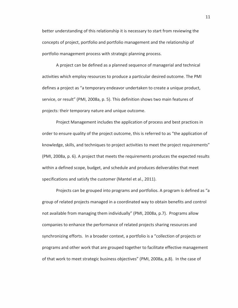
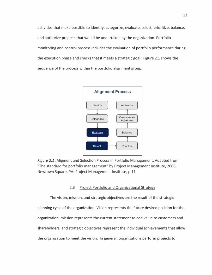
the execution phase and checks that it meets a strategic goal. Figure 2.1 shows the
sequence of the process within the portfolio alignment group.
Figure 2.1 . Aligment and Selection Process in Portfolio Management. Adapted from “The standard for portfolio management” by Project Management Institute, 2008, Newtown Square, PA: Project Management Institute, p.11.
2.3 Project Portfolio and Organizational Strategy
The vision, mission, and strategic objectives are the result of the strategic
planning cycle of the organization. Vision represents the future desired position for the
organization, mission represents the current statement to add value to customers and
shareholders, and strategic objectives represent the individual achievements that allow
the organization to meet the vision. In general, organizations perform projects to
Identify
Categorize
Select Prioritize
Balance
CommunicateAdjustment
Authorize
Alignment Process
EvaluateEvaluateEvaluate
SelectSelect
14
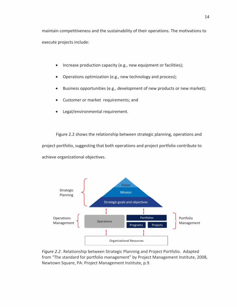
maintain competitiveness and the sustainability of their operations. The motivations to
execute projects include:
Increase production capacity (e.g., new equipment or facilities);
Operations optimization (e.g., new technology and process);
Business opportunities (e.g., development of new products or new market);
Customer or market requirements; and
Legal/environmental requirement.
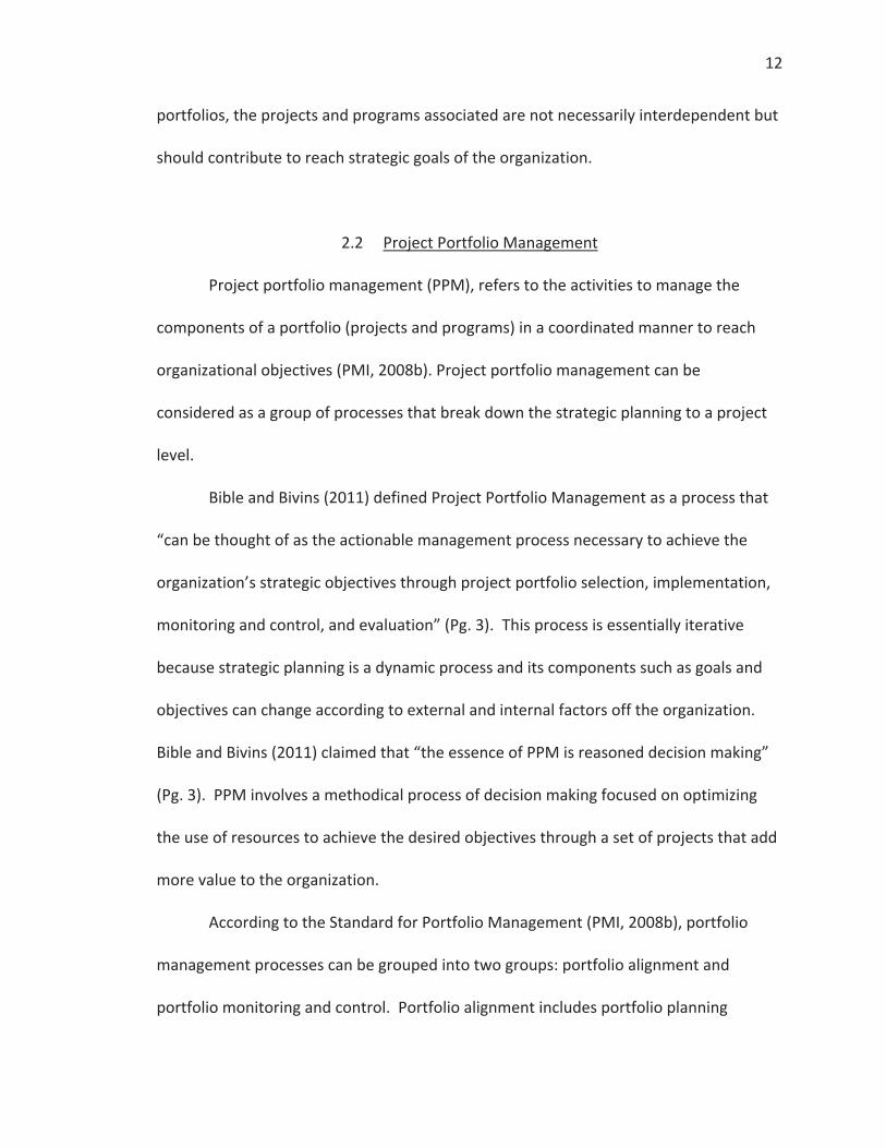
Figure 2.2 shows the relationship between strategic planning, operations and
project portfolio, suggesting that both operations and project portfolio contribute to
achieve organizational objectives.
Figure 2.2 . Relationship between Strategic Planning and Project Portfolio. Adapted from “The standard for portfolio management” by Project Management Institute, 2008, Newtown Square, PA: Project Management Institute, p.9.
Vision
Mission
Strategic goals and objectives
Portfolios
Programs ProjectsOperations
Organizational Resources
Operations Management
l
Strategic Planning
Portfolio Management
15
Archer and Ghasemzadeh (2004) claimed “to ensure a maximum return on
selected projects, the selection process must be linked to the business strategy of the
organization” (pg. 237). Project selection process is a critical phase of portfolio
management and constitutes one of the subjects of research of this proposal.
2.4 Project Success and Portfolio Management
Project success is an important concept in the theory and practice of project
management in organizations. Performance of project managers, project management
teams, and their organizations is usually measured according to success of the projects
in which they are stakeholders. People involved in program and portfolio management
also need to understand the concept of how project success is defined because program
and portfolio success can be considered an aggregate result of project success (Judvev &
Muller, 2005).
The notion of project success has evolved in the last decades and now is
considered a concept that includes some important interrelated dimensions: technical,
economic, behavioral, business and strategic dimensions (McLeod, Doolin & MacDonell,
2012). The evolution in the concept of project success is the result of the analysis of the
lesson learned from projects executed in many organizations and the satisfaction level
of the stakeholders. The following paragraphs discuss the concept of project success in
the context of project/portfolio management and in the context of project/product
lifecycle.
16
2.4.1 Project Success and Project and Portfolio Management
From the project management perspective, the performance of a project is
usually measured by the degree to which the project is completed according the
specified cost, time and scope (Mantel et al., 2011). The scope consists of the
deliverables of the project according to specifications required by the customer. These
specifications include features, performance and quality levels. The cost and time
(schedule) are defined during the project planning phase. Finally, the baselines of scope
cost and time are formally approved by the customer and sponsor before the execution
phase.
Even with a good project planning process, uncertainty during project execution
can make it difficult to deliver the project according to the initial budget, schedule and
scope specifications. Bible and Bivins (2011) claimed that “project management is the
business of meeting the triple constraints of schedule, cost and quality, while at the
same time, producing deliverables that meet specifications and satisfy the customer”
(Pg. 1). These factors are related in such a way that if any one changes, at least one
other factor is affected.
The project team is the one who “assesses the situation and balances the
demands in order to deliver a successful project” (PMI, 2008a, p.7). However, meeting
the triple constraint or, in other words, completing projects on time, within budget and
specified scope, has little value if the projects do not contribute to the achievement of
the organization’s strategic objectives (Bible & Bivins, 2011).

17
Project portfolio management has as a main purpose to link projects and
programs to the goals and strategy of the organization, and optimizing the use of
resources. Bible and Bivins (2011) claimed that “not only do organizations want to
complete the projects successfully by doing the work right, but they also want to
successfully complete the right projects“(Pg. 2). Efficiency is associated with doing the
things right and effectiveness with doing the right things (Judvev & Muller, 2005).
Figure 2.3 represents the integration of these factors in the definition of project success
and integration of project management and portfolio management.
Figure 2.3 . Project Management Successful Factors. Relationship among the Triple Constraint, Project Mangament and Portfolio Management.
In summary, project management is focused in doing things right while portfolio
management is focused on doing the right things (Bible & Bivins, 2011) and a truly
successful project should meet the triple constrain (scope, time and cost) and add value
to the organization, that is, contribute to the achievement of its strategic goals.
Scope
Costost Time
Contribution to organizational objectives
Project Management (Efficiency)
Portfolio Management (Effectiveness)
Customer Satisfaction
18
2.4.2 Project Success and Project and Product Lifecycle
PMI (2008a) defines the product life cycle as:
a collection of generally sequential and sometimes overlapping projects phases
whose name and number are determined by the management and control need
of the organization or organizations involved in the project, the nature of the
project itself, and its area of application. (p.7)
The project life cycle involves all the activities needed to produce the
deliverables of the project. The PMI describes project life cycle as an element of product
life cycle which includes conception, development, operation and finally
decommissioning or withdrawal of a product or process (PMI, 2008a, p.7). Project
portfolio management extends project success beyond the project lifecycle, so project
success can be viewed as an integrated and holistic result.
Shenhar et al (2002) proposed a comprehensive framework that defines four
dimension of project success. The first dimension, associated with the project life cycle,
includes meeting the triple constraint (i.e., scope, time, and budget). The second
dimension measures the benefit for the customer (i.e., fulfill customer needs, customer
satisfaction, use of the product/service). The third dimension measures the benefit for
the organization and it is related with competitiveness (achieve commercial success,
increase market share) and finally, a fourth dimension measures the impact on the
future of the organization (development of new products, technology and new market).
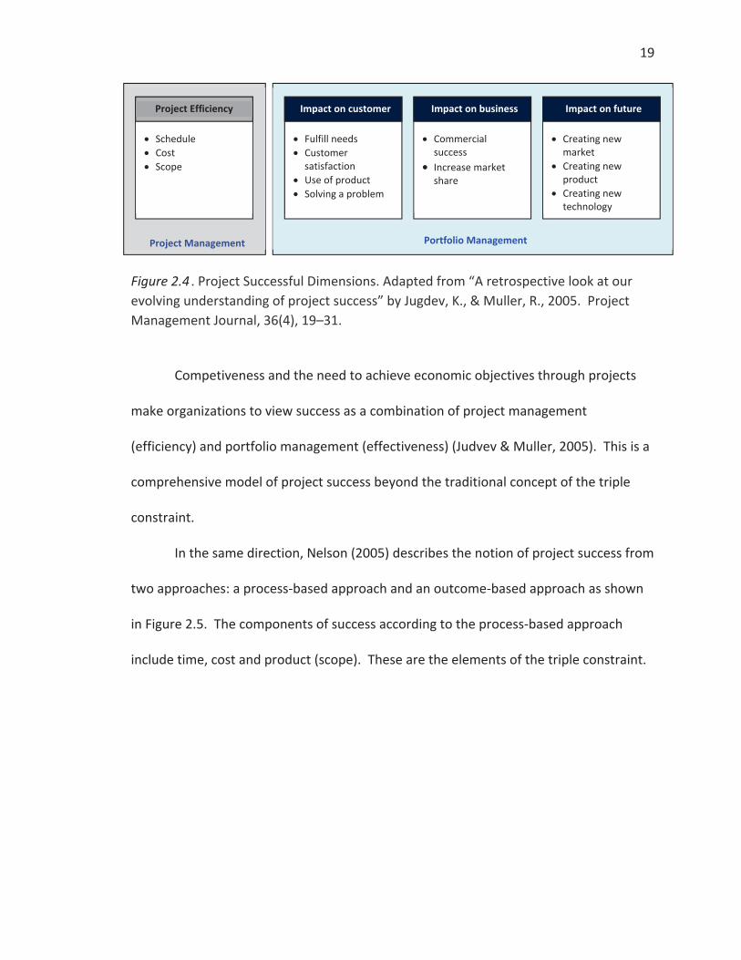
Figure 2.4 shows these dimensions, the critical successful factors associated and the
domain of project and portfolio management.
19
Figure 2.4 . Project Successful Dimensions. Adapted from “A retrospective look at our evolving understanding of project success” by Jugdev, K., & Muller, R., 2005. Project Management Journal, 36(4), 19–31.
Competiveness and the need to achieve economic objectives through projects
make organizations to view success as a combination of project management
(efficiency) and portfolio management (effectiveness) (Judvev & Muller, 2005). This is a
comprehensive model of project success beyond the traditional concept of the triple
constraint.
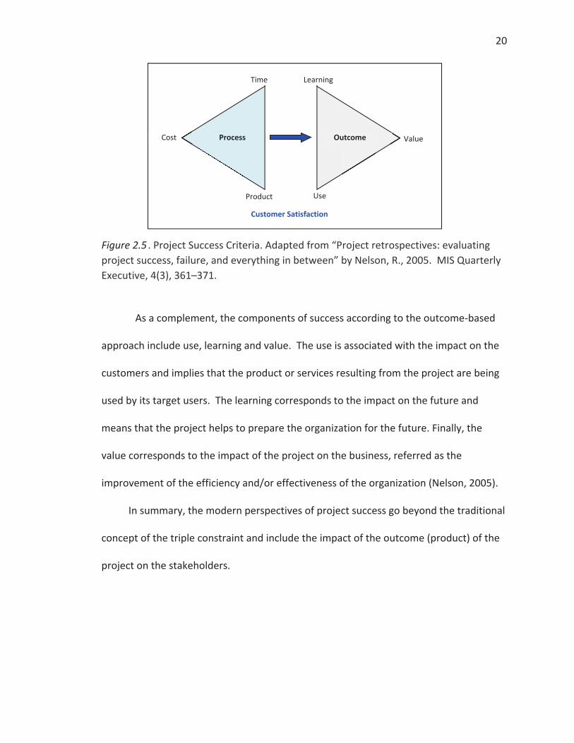
In the same direction, Nelson (2005) describes the notion of project success from
two approaches: a process-based approach and an outcome-based approach as shown
in Figure 2.5. The components of success according to the process-based approach
include time, cost and product (scope). These are the elements of the triple constraint.
Project Management
Portfolio Management
Schedule Cost Scope
Project Efficiency
Fulfill needs Customer satisfaction Use of product Solving a problem
Impact on customer
Commercial success Increase market share
Impact on business
Creating new market Creating new product Creating new technology
Impact on future
20
Figure 2.5 . Project Success Criteria. Adapted from “Project retrospectives: evaluating project success, failure, and everything in between” by Nelson, R., 2005. MIS Quarterly Executive, 4(3), 361–371.
As a complement, the components of success according to the outcome-based
approach include use, learning and value. The use is associated with the impact on the
customers and implies that the product or services resulting from the project are being
used by its target users. The learning corresponds to the impact on the future and
means that the project helps to prepare the organization for the future. Finally, the
value corresponds to the impact of the project on the business, referred as the
improvement of the efficiency and/or effectiveness of the organization (Nelson, 2005).
In summary, the modern perspectives of project success go beyond the traditional
concept of the triple constraint and include the impact of the outcome (product) of the
project on the stakeholders.
Time
Product
Learning
Use
Value
Customer Satisfaction
Process Outcome Cost
21
2.5 Project Portfolio Selection Methods
Project evaluation and selection are important processes in the portfolio
management activities of the organization. Portfolio selection is a process that involves
the assessment of a set of available project proposals in order to undertake a group of
them that makes it possible to achieve some strategic goals (Mantel et al., 2011).
Portfolio selection is a periodic process that must guarantee that the selected projects
are inside the resource constraints of the organization (Ghasemzadeh & Archer, 2000).
The objective of the project selection process is to derive a portfolio of projects
providing maximum benefit subjected to resources constrains and other limitations
imposed by the organizations (Bible and Bivins, 2011). Portfolio selection seeks the best
balance in terms of return, capital investment, risk, timing, sustainability, and other
factors according to the organization needs and policies.
Project selection methodologies play an important role in portfolio
management. However, there is a plethora of project selection methodologies, and
there is no agreement on which is the most effective (Archer & Ghasemzadeh, 2004).
Consequently, organizations choose the methodology that best reflects their project
management maturity level, organizational culture, and kind of projects developed.
Mantel et al. (2011) classifies the project selection methods in two categories:
nonnumeric and numeric. The following sections describe the main methodologies for
project selection.
22
2.5.1 Nonnumeric Selection Methods
Nonnumeric selection methods are used in the industry because these methods
are simple and take into consideration the experience and know-how of the decision
makers. Some of these methods are described in the following paragraphs.
2.5.1.1 Sacred Cow
In this approach, a high level executive based on her or his experience,
knowledge, and authority level decides that the organization must develop a specific
project (Mantel et al., 2011). This method is common in many kinds of businesses;
however, resulting decisions might be questionable due to subjective assessment of the
decision maker or poor technical and economic justifications.
2.5.1.2 Operating/Competitive Necessity.
This method selects the projects that are needed to keep the business running
(Mantel et al., 2011). Under certain circumstances, an organization must undertake
some projects to assure its sustainability in the long term.
2.5.1.3 Comparative Models
Comparative models relate one candidate project either to another project or to
some subset of candidate projects, in such a way that the obtained benefits have
meaning only in relation to the set of candidate projects evaluated. Therefore,
whenever a candidate project is added or deleted from the set under evaluation, the
23
entire process must be repeated (Heidenberger & Stummer, 1999). The main
comparative models used in project selection are Q-sort approach and Analytical
hierarchy process (AHP).
2.5.1.3.1 Q-Sort
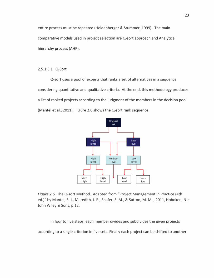
Q-sort uses a pool of experts that ranks a set of alternatives in a sequence
considering quantitative and qualitative criteria. At the end, this methodology produces
a list of ranked projects according to the judgment of the members in the decision pool
(Mantel et al., 2011). Figure 2.6 shows the Q-sort rank sequence.
Figure 2.6 . The Q-sort Method. Adapted from “Project Management in Practice (4th ed.)” by Mantel, S. J., Meredith, J. R., Shafer, S. M., & Sutton, M. M. , 2011, Hoboken, NJ: John Wiley & Sons, p.12.
In four to five steps, each member divides and subdivides the given projects
according to a single criterion in five sets. Finally each project can be shifted to another
Originalset
Highlevel
Lowlevel
Mediumlevel
Highlevel
Lowlevel
Very High
Highlevel
Lowlevel
Verylow
24
set if necessary. This procedure provides flexibility and interaction between the
members of the decision team (Heidenberger & Stummer, 1999).
2.5.1.3.2 The Analytic Hierarchy Process (AHP)
The analytic hierarchy process is a multicriteria decision making model that can
use both qualitative and quantitative factors and is based on pair-wise comparison by
which the judgment of experts produces a recommendation. As project selection is a
decision making process, AHP can be used as a project selection methodology (Saaty,
2008).
AHP allows a decision maker to structure a project evaluation in the form of a
hierarchy with the projects at the bottom and the various criteria (or objectives) at
respective higher levels. At any level, each alternative has the same order of magnitude
or importance and is evaluated in relation to its peers with respect to its importance for
the objectives immediately above. Pairwise cardinal comparisons lead to a matrix
whose eigenvector contains the weights or priorities. This process is repeated for all
levels in the hierarchy. Then, the matrices of eigenvectors that summarizes the
priorities between levels are multiplied to finally determine the compound priorities of
the project alternatives according to their influence on the overall goal of the hierarchy
(Heidenberger & Stummer, 1999).
There are many examples in the literature that show the application of AHP in
project selection problems. Dey (2006) applied AHP for a project selection case study of
a cross-country petroleum pipelines project in India. This case includes identification of
25
alternatives, identification of factors to be considered (technical, environmental, and
socio- economic criteria), creation of the AHP framework for deployment of the main
and secondary decision factors according to each criteria, comparison of pairwise
alternatives for each factor and, finally, aggregating the results.
An advantage of AHP models is that both quantitative and qualitative criteria can
be used. A major disadvantage is the large number of comparisons involved, making
them difficult to use in large portfolios. However, the use of computational tools such as
Expert Choice can support the management of large portfolios. Bible and Bivins (2011)
illustrated the use of Expert Choice in Project Portfolio Management activities including
project selection.
Vaidya and Kumar (2006) claimed that “the specialty of AHP is its flexibility to be
integrated with different techniques like Linear Programming, Quality Function
Deployment, Fuzzy Logic, etc” (p.2). This makes it possible to combine AHP with other
project selection models taking advantage of their strengths.
2.5.2 Numeric Selection Methods
Numeric selection methods rate the candidate projects according quantitative
and qualitative normalized criteria. These criteria usually include financial benefits,
productivity, reliability, environmental impact and risks associated with each project
alternative. Numeric methods are used in the industry because these methods can
provide a more accurate assessment of benefits for each candidate project to the
decision maker. Some of these methods are described in the following paragraphs.

26
2.5.2.1 Financial Assessment Models
Traditional economic models attempt to calculate the cost-benefit. These
methods typically require financial estimates of investment and income flows over the
time frame of the project. These models are generally used in construction projects,
where possible estimate costs and schedule are with some accuracy based on
experience in similar projects (Archer & Ghasemzadeh, 2004).
The results of the financial evaluation for different project alternatives can be
used in raking the potential benefits for decision making purpose. Blocher et al. (2010)
described the financial methods for capital investments evaluation according to two
categories: discounted cash flow (DCF) models and non-DCF models.
2.5.2.1.1 Discounted Cash-Flow Methods (DCF)
DFC methods consider the value of money in time and include performance
indicators such as net present value (NPV), internal rate of return (IRR), and profitability
index (PI). NPV is the difference between the present value of cash inflow and outflow
for an investment as calculated in Equation 1 (Mantel et al., 2011). A positive NPV
means the project earns more than the required rate of return and that the project may
be accepted.
(1)
Where: Io is the initial investment
Ft is the net cash flow in the period t

27
k is the required rate of return
n is the number of periods in life of the project
The internal rate of return (IRR) is an estimate of rate of return of the investment
that produces NPV zero. The project is accepted if the IRR exceeds the discount rate set
by the organization. The profitability index (PI) is the ratio between net present values
per invested amount. Equation 2 shows this relationship (Blocher et al., 2010)
(2)
2.5.2.1.2 Non-Discounted Cash-Flow Methods
Non-DFC methods do not consider the value of money in time; however they can
be used to prescreen some project alternatives. The most used non-DCF indicator is the
payback period (PBP), defined as the time required for the cumulative cash inflow
(after-tax) to recover the initial investment. PBP is considered a measure of risk of
investment, longer PBP means higher risk to the organization. Equation 3 shows how to
determine the PBP with uniform annual net cash inflow (Mantel et al., 2011).
(3)
Where: F is the estimated annual net cash inflow

28
Financial methods are broadly employed. Blocher et al. (2010) claimed that
three of four firms use both NPV and IRR for capital-budgeting purposes. All these
financial methodologies are powerful tools to evaluate the economic benefits of a
project; however, they ignore non-financial considerations, such as social or
environmental impact.
2.5.2.2 Scoring Methods
Scoring methods consider more than one criterion and can combine qualitative
and quantitative factors. Some advantages of these models are that they are probably
the easiest to use of all methods and, that projects can be added or deleted from the set
without recalculating the score of other projects (Archer & Ghasemzadeh, 2004).
Scoring methods include the unweighted and the weighted factor scoring method.
2.5.2.2.1 The Unweighted 0-1 Factor Model (or Checklist Approach)
This model lists some factors which are desirable for the projects under review
and a decision committee checks off which criteria are satisfied (Mantel et al., 2011).
The score is related to the number of criteria the alternative meets and can be
calculated according to Equation 4 (Heidenberger & Stummer, 1999):
(4)
(5)
29
Where: Si is the total score of the ith project
sij is the score of the ith project on the jth criterion
This method assumes that all criteria are equally important. In case this
assumption is not true, the ranking may be misleading.
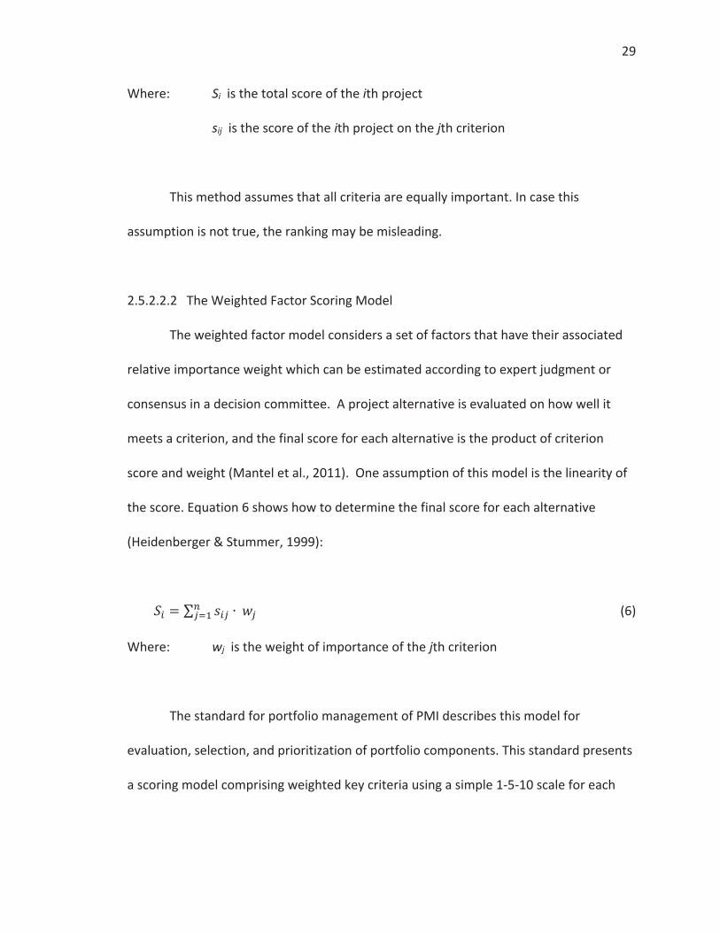
2.5.2.2.2 The Weighted Factor Scoring Model
The weighted factor model considers a set of factors that have their associated
relative importance weight which can be estimated according to expert judgment or
consensus in a decision committee. A project alternative is evaluated on how well it
meets a criterion, and the final score for each alternative is the product of criterion
score and weight (Mantel et al., 2011). One assumption of this model is the linearity of
the score. Equation 6 shows how to determine the final score for each alternative
(Heidenberger & Stummer, 1999):
(6)
Where: wj is the weight of importance of the jth criterion
The standard for portfolio management of PMI describes this model for
evaluation, selection, and prioritization of portfolio components. This standard presents
a scoring model comprising weighted key criteria using a simple 1-5-10 scale for each
30
criterion and then evaluating components according to groups of criteria. The sum of
the weights of the criteria should be 100% (PMI, 2008b).
The weighed factor scoring model is broadly used in the industry because this
model considers multiple criteria, is ease to implement and understand by the decision
makers. However, this model have the following drawbacks:
The problem of weights assignment is not considered in this model and could be
subject to the interests of the persons involved in the process. This problem
could be solved by integrating a group decision making technique such as AHP
for weights assignment.
Scoring models do not consider any type of relationship between candidate
projects and this could be important in some problems of project selection with
dependent or mutually exclusive projects.
Scoring models do not guarantee the optimal allocation of the resources of the
organization because these models do not include resource constraint.
The reliability of the values for each alternative is not considered. This might be
a source of risk in the decision making process.
There are numerous examples of the application of weighted factor scoring
methods in different kinds of projects and industry sectors. Sarkis, Presley, and Liles
(1997) illustrated a framework for strategic multi-attribute evaluation for business
process reengineering (BPR) projects. In this work, a link between the projects and the
strategic goals of the organization is established. Three types of strategic metrics

31
categories are used in the analysis: financial, quantitative, and qualitative criteria. The
scores for each criterion are normalized using linear utility functions. Finally, weights of
criteria are assigned for a decision team.
Strang (2011) showed an action research case study using a weighted multi-
criteria scoring model in a selection process of technical proposals for a project in a
nuclear facility. This model applies AHP to estimate the weights of criteria and the
transformation of original-scaled values into dimensionless values to get the total score
of each alternative. The case study considers some important elements in the decision
process such as estimation of the factor weights using AHP, which considers the opinion
of experts and reliability factors for the values of the main variables for each project.
2.5.2.3 Optimization Models
Optimization models are based on operation research tools and use some form
of mathematical programming to select a set of projects which deliver maximum benefit
(e.g., NPV, profit) represented for and objective function subjected to a series of
constraints (e.g., cost, people). There are some cases in the literature about using
optimization models combined with some of the other models mentioned before. For
example, Schniederjans and Wilson (1991) showed a model using goal programming and
AHP while Lee and Kim (2000) showed an application of goal programming and
Analytical Network Process (ANP). However, Archer and Ghasemzadeh (2004) claimed
that the use of mathematical programming models in the practical is not generalized
because they can be highly complex and require a significant amount of data.
32
The next section describes the use of mathematical programming models with
some detail and emphasizes the mathematical formulation of the model including the
definition of the decision variables, objective function and the most relevant
constraints: resource constraints, technical requirements and interdependence among
projects.
2.6 Mathematical Programming Models for Project Selection
The basic objective of mathematical programming problem is to maximize or
minimize an objective function and meet some constraints. The formulation of the
linear programming problem includes defining decision variables, objective function,
and constraints. There are many forms of mathematical programming for optimization
including linear and non-linear programming, integer programming, goal programming,
dynamic programming and stochastic programming (Heidenberger & Stummer, 1999).
Nonetheless, two approaches seem to be more suitable and easy to apply in project
selection problems: Integer linear programming model when the decision maker is
focused on optimizing one objective and goal programming model when the decision
maker considers satisfying multiple objectives.
2.6.1 Integer Linear Programming Models (ILP)
The integer programming model selects a set of projects which maximize a
benefit (objective). This section focuses on the formulation of project selection
problems using integer programming and considering two cases: in the first one, it is
33
assumed the projects are executed at the same time, so the resources are available to
be used by the selected projects in one period of time. In the second case, project
selection and scheduling during a time horizon is considered, so the projects can be
executed in different moments according to resources availability during each period
and relationship between candidate projects.
2.6.1.1 0-1 ILP Project Selection without Scheduling (Single Period)
This model is the most simplified approach and assumes all resources are
available to execute the selected candidate projects at the same time (a single period),
that is, the resources are available to be used for simultaneous project execution. This
problem known as Capital Budgeting Problem, is described in Chen, Batson and Dang
(2010) and the formulation is shown in Equations (7) to (9). This model considers n
candidate projects and each project i have an associated decision variable which is
defined as follows:
(7)
for i = 1, …, n, where n is the total number of projects being considered
The objective function Z is the total benefit of any project set. The solution seeks
to maximize Z as follows:
34
(8)
Where: Z is the criterion to be maximized and corresponds to the total benefit of the
portfolio. Usually Z is the overall NPV of the portfolio.
ci is the benefit provided by the project i
Constrains are functions that consider the availability of resources (money,
people, facilities, etc.) for project execution or describe some requirements (technical,
environmental, etc.) that projects must meet. In general, resources constraints can be
defined by Equation 9.
(9)
Where aij is the use of resource j by project i and bj is the availability of resource j to be
used for execution of the project portfolio. In the case of constraints related with
requirements, these constraints can be represented by an inequality (≥ or ≤) or a strictly
equal (=) constraint.
Integer programming models can consider interdependent projects within a
portfolio such as contingent projects, mutually exclusive projects, parallel and
mandatory projects (Heidenberger & Stummer, 1999). These conditions are described
by using constraints equations relating candidate projects. For example, consider the
case of dependent projects where if project j is selected, then project i must also be

35
selected, but the opposite is not a condition. This circumstance is described by Equation
10 (Winston & Venkataramanan, 2003).
(10)
The case of mutually exclusive projects (i.e., if project j is selected, then project i
cannot be selected) is described by Equation 11 (Winston & Venkataramanan, 2003):
(11)
Finally, if project i is mandatory and its execution affects the amount of
resources available for other candidate projects, it must be included in the project
selection model using Equation 12 (Winston & Venkataramanan, 2003):
(12)
2.6.1.2 0-1 ILP Project Selection With Scheduling (Multiple Periods)
More complex models can consider the starting time and duration of the
candidate projects in the decision variables (Heidenberger & Stummer, 1999). This is a
more real approach to portfolio management in corporate environments and can be
used for the optimal distribution of the resources over the planning horizon when a
project portfolio should be executed. Ghasemzadeh, Archer, and Iyogun (1999) present
a model for project selection and scheduling using zero-one linear programming. The
36
basic formulation is shown in Equations 13 and 14. This model considers n candidate
projects and t periods of time. The decision variables are defined as follows:
(13)
for i = 1, …, n, where n is the total number of projects being considered
j = 1, …, t, where t is the total number of periods in the planning horizon.
The objective function Z is the total benefit of any project set. The solution seeks
to maximize Z as follows.
(14)
Where: Z is the criterion to be maximized and corresponds to the total benefit of the
portfolio and is related to the organizational goals. Usually Z is the overall
NPV of the portfolio.
ci is the benefit provided by the project i
The inclusion of time for starting a project implies the use of some set of
constraints to control the flow of execution, the availability of resources in each period j
and the interdependence relationship of some candidate projects. The constraint
represented in Equation 15 ensures that each project, if selected, will be started only
once during the planning horizon (Ghasemzadeh, Archer, & Iyogun, 1999).

37
for i = 1, …, n (15)
Another important condition is that all selected projects should be finished
within the planning horizon. In this case, all projects selected should be finished by the
end of period t. This is described in Equation 16 (Ghasemzadeh, Archer, & Iyogun, 1999):
for i = 1, …, n (16)
Where di is the duration of project i (number of periods required to be completed)
The availability of resources (e.g., financial resources, machinery, workforce)
may vary during the planning horizon. For example, the organization may have
availability of financial resources according to cash flow (budget). This set of constraints
is shown in Equation 17 (Ghasemzadeh, Archer, & Iyogun,1999):
for k = 1, …, t (17)
Where bk is the cumulated amount of resource available in period k and ak+1-j is the
cumulated amount of resources required by project i in the period k.
In a project portfolio selection, it is possible to consider interdependence among
candidate projects, such as complementary, mutually exclusive and mandatory projects.
The modeling of this constraints are shown in Equations 18, 19 and 20 (Ghasemzadeh,
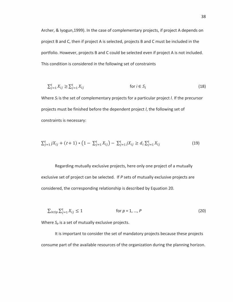
38
Archer, & Iyogun,1999). In the case of complementary projects, if project A depends on
project B and C, then if project A is selected, projects B and C must be included in the
portfolio. However, projects B and C could be selected even if project A is not included.
This condition is considered in the following set of constraints
for i (18)
Where Sl is the set of complementary projects for a particular project l. If the precursor
projects must be finished before the dependent project l, the following set of
constraints is necessary:
(19)
Regarding mutually exclusive projects, here only one project of a mutually
exclusive set of project can be selected. If P sets of mutually exclusive projects are
considered, the corresponding relationship is described by Equation 20.
for p = 1, …, P (20)
Where Sp is a set of mutually exclusive projects.
It is important to consider the set of mandatory projects because these projects
consume part of the available resources of the organization during the planning horizon.
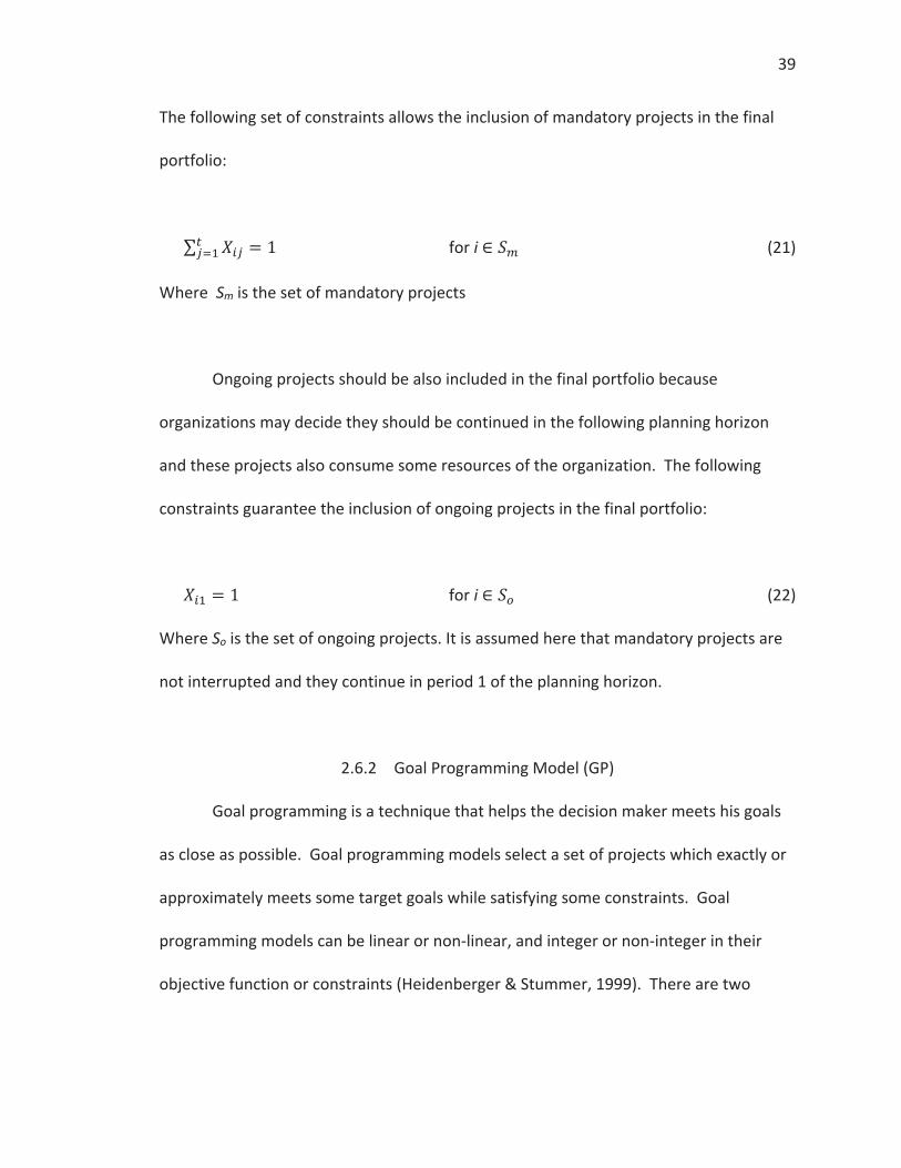
39
The following set of constraints allows the inclusion of mandatory projects in the final
portfolio:
for i (21)
Where Sm is the set of mandatory projects
Ongoing projects should be also included in the final portfolio because
organizations may decide they should be continued in the following planning horizon
and these projects also consume some resources of the organization. The following
constraints guarantee the inclusion of ongoing projects in the final portfolio:
for i (22)
Where So is the set of ongoing projects. It is assumed here that mandatory projects are
not interrupted and they continue in period 1 of the planning horizon.
2.6.2 Goal Programming Model (GP)
Goal programming is a technique that helps the decision maker meets his goals
as close as possible. Goal programming models select a set of projects which exactly or
approximately meets some target goals while satisfying some constraints. Goal
programming models can be linear or non-linear, and integer or non-integer in their
objective function or constraints (Heidenberger & Stummer, 1999). There are two

40
approaches of goal programming that can be applied to the project selection problem,
depending how the decision maker values the importance of the target goals and the
way the objective function is defined: weighted and lexicographic goal programming.
2.6.2.1 Weighted Goal Programming Without Scheduling (Single Period)
The general goal programming formulation is shown by Jones and Tamiz (2010).
A specific formulation for the project selection problem developed by the author of this
research is shown in Equations 23 through 25. This model considers n candidate
projects, m goals and some constraints. Each project i has an associated decision
variable which is defined by Equation 23.
(23)
For i = 1, 2, …, n, where n is the total number of projects being considered.
Each goal p has associated a target value gp and a goal weight Wp according its
relative importance. Any possible solution (set of projects) has two deviational variables
defined as follows:
Sep : amount by which the project set numerically exceeds the pth goal
Sup : amount by which the project set is numerically under the pth goal
The objective function Z is the total deviation of the any project set from the
goals. The solution seeks to minimize Z as follows:
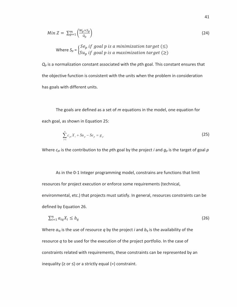
41
Qp (24)
Where Sp =
Qp is a normalization constant associated with the pth goal. This constant ensures that
the objective function is consistent with the units when the problem in consideration
has goals with different units.
The goals are defined as a set of m equations in the model, one equation for
each goal, as shown in Equation 25:
ppp
n
iipi gSeSuXc
1
(25)
Where cpi is the contribution to the pth goal by the project i and gp is the target of goal p
As in the 0-1 Integer programming model, constrains are functions that limit
resources for project execution or enforce some requirements (technical,
environmental, etc.) that projects must satisfy. In general, resources constraints can be
defined by Equation 26.
(26)
Where aiq is the use of resource q by the project i and bq is the availability of the
resource q to be used for the execution of the project portfolio. In the case of
constraints related with requirements, these constraints can be represented by an
inequality (≥ or ≤) or a strictly equal (=) constraint.
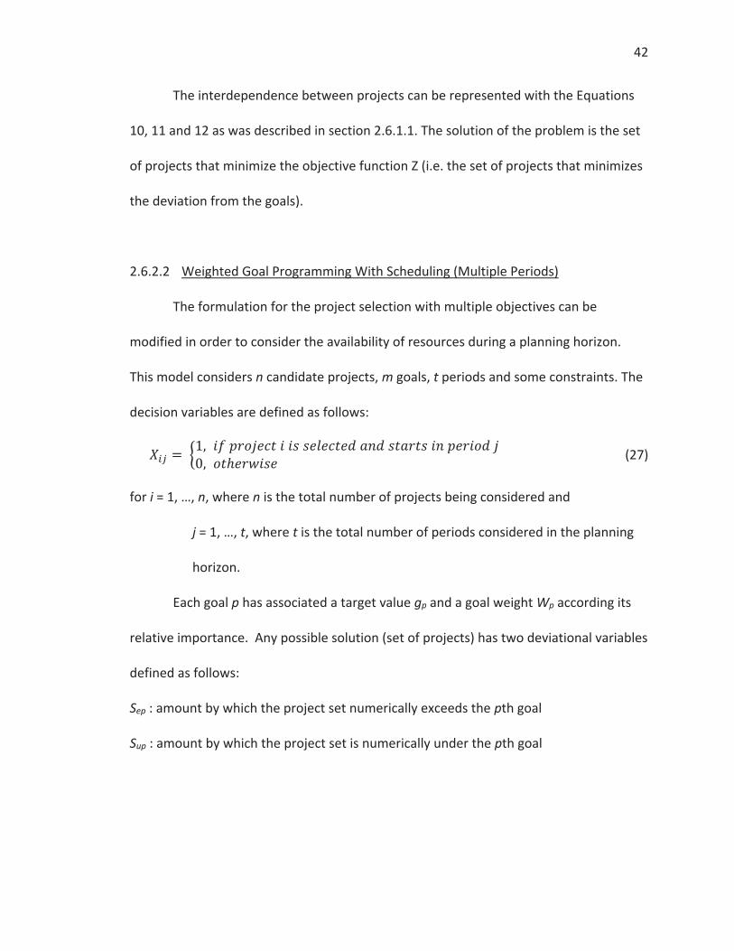
42
The interdependence between projects can be represented with the Equations
10, 11 and 12 as was described in section 2.6.1.1. The solution of the problem is the set
of projects that minimize the objective function Z (i.e. the set of projects that minimizes
the deviation from the goals).
2.6.2.2 Weighted Goal Programming With Scheduling (Multiple Periods)
The formulation for the project selection with multiple objectives can be
modified in order to consider the availability of resources during a planning horizon.
This model considers n candidate projects, m goals, t periods and some constraints. The
decision variables are defined as follows:
(27)
for i = 1, …, n, where n is the total number of projects being considered and
j = 1, …, t, where t is the total number of periods considered in the planning
horizon.
Each goal p has associated a target value gp and a goal weight Wp according its
relative importance. Any possible solution (set of projects) has two deviational variables
defined as follows:
Sep : amount by which the project set numerically exceeds the pth goal
Sup : amount by which the project set is numerically under the pth goal
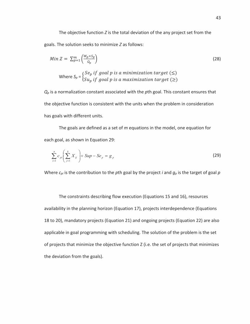
43
The objective function Z is the total deviation of the any project set from the
goals. The solution seeks to minimize Z as follows:
Qp (28)
Where Sp =
Qp is a normalization constant associated with the pth goal. This constant ensures that
the objective function is consistent with the units when the problem in consideration
has goals with different units.
The goals are defined as a set of m equations in the model, one equation for
each goal, as shown in Equation 29:
pp
k
jij
n
ipi gSeSupXc
11
(29)
Where cpi is the contribution to the pth goal by the project i and gp is the target of goal p
The constraints describing flow execution (Equations 15 and 16), resources
availability in the planning horizon (Equation 17), projects interdependence (Equations
18 to 20), mandatory projects (Equation 21) and ongoing projects (Equation 22) are also
applicable in goal programming with scheduling. The solution of the problem is the set
of projects that minimize the objective function Z (i.e. the set of projects that minimizes
the deviation from the goals).

44
2.6.2.3 Lexicographic Goal Programming
Lexicographic goal programming (or preemptive goal programming) does not use
weighted criteria but a number of priority levels, that is, the algorithm seeks to satisfy
first the goal with the highest priority, and then continues with the second more
important and so on. The decision maker assigns the level of importance P for each goal.
If k is the number of goals and each goal has a priority level, then the objective function
can be described as follows (Jones & Tamiz, 2010):
(30)
Qj (31)
Where Sj =
Pj is the priority factor associated with the jth goal
Qj is a normalization constant associated with the jth goal
The priority factors are defined in such a way that the satisfaction of the set of
goals of higher priority is much more important than the satisfaction of sets of goals of
lower priority (Heidenberger & Stummer, 1999). The decision maker must rank the goals
from the most important (goal 1) to the least important (goal k). The priority factor
associated with the jth goal is such that:
45
(32)
The definition of the priority factors ensure that the algorithm tries to satisfy the
most important goal (goal 1) first, then using the feasible points that satisfy goal 1, it
tries to come as close as possible to satisfying goal 2, and so forth (Winston &
Venkataramanan, 2003). The equations for the goals and constraints are the Equations
25 and 26 shown for the weighted goal programming formulation.
There are some examples of project selection models using goal programming.
Lee and Kim (2000) showed a methodology for project selection that uses a zero-one
goal programming model for information system (IS) projects, which objective is
minimizing the costs associated with several projects that have some interdependency.
In this application, Analytical Network Process (ANP) is used to determine the relative
importance of the criteria considered.
2.6.3 Solution of Mathematical Programming Models
The solution of mathematical programming problems is a topic of intense study
in the field of math and operations research. As the problems become more complex
with many variables and constraints, the efficiency and robustness of the algorithms to
solve the problems are a critical factor for its implementation in a computational tool.

46
2.6.3.1 Algorithm for Solving Mathematical Programming Problems
The solution of the set of equations is the set of projects that maximizes the
objective function Z. This corresponds to the set of projects that maximizes the benefit.
Linear programming problems are usually solved applying simplex or Karmakar’s
algorithm and integer linear programming problems are solved using branch-and-bound
or cutting plane algorithm (Winston & Venkataramanan, 2003).
2.6.3.2 Solution of Mathematical Programming Problems with Software
The increasing application of mathematical programming in many areas in
business (e.g., production scheduling, inventory, logistics) and the formulation of more
complex problems (e.g., large number of variables and constraints) have made
indispensable the use of specialized software. In the last decades, both the
development of more efficient algorithms and the increasing capacity of processors
have made possible the solution of large-scale mathematical programming in a
reasonable time.
In order to solve a problem of optimization, the first step is the formulation that
translates the real world problem in algebraic language defining the decision variables,
objective function and constraints. After a model is formulated, a computer package is
used to solve the problem. During this step, the programmer must translate the
formulation into a code that the software can recognize. According to Chen, Batson and

47
Dang (2010) the main components of a software for mathematical programming include
modeling language, presolver, solver and the data and application interface.
1. Modeling languages emerged in the mid-to late 1980s and introduced the use of
sets, symbolic parameters, indexed variables and constraints, operators and
control flow commands. The modeling languages makes possible to define a
symbolic algebraic model of the problem, by keeping separated the model and
the data. This feature allows running the model with different set of data
creating instances of the same problem and comparing results. The modeling
language works as two-way communication channel between user and solver,
that is, it communicates the data from the user to the solver and the results from
the solver to the user (Chen, Batson & Dang, 2010). Among the most popular
algebraic modeling languages are AMPL, GAMS, MPL, LINGO, and AIMMS.
2. The presolver applies preprocessing techniques in order to get a better
formulation that is easier to solve. The preprocessing techniques, which depend
on the kind of algorithm to be applied, adjust the variables and constraint in
order to increase the computational efficiency (Chen, Batson & Dang, 2010).
3. The solver receives the model from the algebraic modeling language and tries to
find an optimal solution for a particular set of data applying the more convenient
algorithm according to the kind of problem. For example linear programming
(LP) problems are solved using the simplex algorithm, while integer (IP) and
mixed integer (MIP) problems can be solved using branch and bound algorithm
48
(Winston & Venkataramanan, 2003). Among the most used solvers used for MIP
are CPLEX, GUROBI, MOSEK, BARON, CBC and XA.
4. Data and application interfaces are more critical when the model requires a
significant amount of data. The modeling language can read data from external
structured data sources such as databases, spreadsheets or simple text files to
generate a matrix that the solver can use to run the solution algorithm.
Application interfaces (APIs) developed in commercial programming languages
as Java or C++ allow to call modeling languages and solvers from customized
applications (Chen, Batson & Dang, 2010).
Some modeling languages incorporate a presolver, a data interface and solvers
from different solver providers in order to offer an integrated environment of
application software development. A list of the main commercial modeling languages
and solvers are published by INFORMS (Fourer, 2013, June).
2.7 Project Portfolio Selection with Commercial Software
The project portfolio selection problem is part of the planning cycle of many
organizations. There is some commercial software that assists the decision maker in this
task. Most of these commercial software offer comprehensive suite for Project Portfolio
Management (PPM) and the component for project selection is just a part of the
package, they require a considerable investment and specialized training for the users.
These commercial software are usually based on any of the methods described in
49
section 2.5. In the next paragraphs there is a description of some of the commercial
software that support the project selection process.
Expert Choice Comparion. The use of this software for portfolio selection is
illustrated in detail in Bible and Bivins, (2011). This application is a web-based
decision making tool based on Analytical Hierarchy Process (AHP). This tool
allows a decision making team to facilitate the collaboration and structure
decisions based on quantitative and qualitative data. In the case of project
portfolio selection, the decision makers should have identified a main goal of the
portfolio, a list of objectives associated to that goal and a group of alternatives
(candidate projects). In the first step, the participants have to make a series of
pairwise comparisons to provide judgments about the relative importance of the
objectives. After all objectives have been compared to each other, the objective
priorities for each participant are calculated. In the next step, the participant
should rate how well each alternative contributes to each of the objectives.
Expert Choice provides different ways to compare the goals and rate alternatives
including numerical, verbal and graphical methods. In the final step, after all the
participants have rated objectives and alternatives, Expert Choice combines and
synthesizes the results to produce an overall ranking. Expert Choice allows
making a sensitivity analysis by changing the relative priorities of the objectives
to see how the portfolio changes (Expert Choice, 2014).
50
GenSight. This application is a fully integrated web-based portfolio management
system. This software includes forms to enable the capture of the business case,
extensive workflow capabilities for the study, approval and execution of the
portfolio components, decision support tools to prioritize projects and support
approval gates. GenSight supports all common financial analysis including
profitability, NPV, ROI, etc. Project selection is based on weighted multi-criteria
methods. GenSight includes utility functions to normalize diverse quantitative
metrics, qualitative utility scales and pairwise comparison. The Portfolio Analyst
Workbench is a tool of GenSight that works offline and provides 2D and 3D
graphical visualization and ‘what if’ scenario planning. Finally the GenSight
Optimizer is a tool that incorporates proprietary genetic optimization algorithm
to find the best combination of portfolio elements to maximize the return from
constrained resources or assets. This tool is packaged as an optional add-on
module to the Portfolio Analyst Workbench (The GenSight group, 2011).
CANEA Projects. This software, developed in Sweden, integrates project,
portfolio and resource management with support for the whole organization.
CANEA Projects can be integrated with CANEA Improof, a workflow solution for
many types of administrative processes, and CANEA Docpoint, a document
management system for all the components associated with a Portfolio. CANEA
Projects enables the selection and prioritization of projects using scoring models
(CANEA Consulting Group, 2011).
51
2.8 Case Study: Project Portfolio Selection in Cementos Argos
This study included a case study of project portfolio selection in Cementos Argos,
the main Colombian Portland cement producer, with an extensive portfolio including
projects in industrial facilities for increasing production, operations optimization,
projects that allow compliance of environmental regulations, projects aims improving
the supply chain and logistics, etc.
This section contains a summary about Portland cement as product, the Portland
cement production process and a description of Cementos Argos as a company. The
purpose of this case study is to evaluate the improvement in the quality of the proposed
portfolio when using the DSS for project selection vs. using the Argos’s current selection
method. This corresponds to the first research question that aims develop a model
which finds the best portfolio for an organization. The data and results of this case study
are presented in detail in chapter 4.
2.8.1 Portland Cement
The American Society for Testing and Materials (ASTM, 2012) defines Portland
cement as:
hydraulic cement (cement that not only hardens by reacting with water but also
forms a water-resistant product) produced by pulverizing clinkers consisting
essentially of hydraulic calcium silicates, usually containing one or more of the
forms of calcium sulfate as an interground addition.

52
Portland cements is the most common type of cement and the basic constituent
of concrete, mortar, stucco and grout.
According the Portland Cement Association, Portland cement was originally
developed and patented in England by Joseph Aspdin of Leeds, early in the 19th century
by burning powdered limestone and clay presenting a texture similar to Portland stone
(PCA, 2014). The Portland cement is a fine powder produced in a chemical process
combining calcium, silicon, aluminum and iron. The materials used to manufacture
cement include limestone or marl (CaCO3) combined with clay (Al2O3), slate, blast
furnace slag or silica sand (SiO2), and iron ore (Fe2O3). The low cost and widespread
availability of these raw materials make Portland cement one of the lowest-cost
materials used in the world (PCA, 2014).
2.8.2 Portland Cement Production Process
Cement production involves physical and chemical processing of raw materials in
specialized equipment that require high investment. Cement production facilities,
located near raw materials sources, require large amount of energy as electrical power
feeding many processing and conveying equipment as well as fuels for drying and
burning raw materials and environmental pollution control equipment. Currently, most
cement is produced in a technology called Dry Process (PCA, 2014). Figure 2.7 and the
following paragraphs describe the production process applied in a modern cement plant
using dry process.
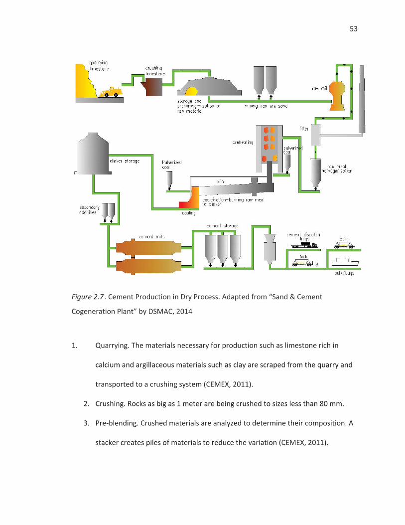
53
Figure 2.7 . Cement Production in Dry Process. Adapted from “Sand & Cement
Cogeneration Plant” by DSMAC, 2014
1. Quarrying. The materials necessary for production such as limestone rich in
calcium and argillaceous materials such as clay are scraped from the quarry and
transported to a crushing system (CEMEX, 2011).
2. Crushing. Rocks as big as 1 meter are being crushed to sizes less than 80 mm.
3. Pre-blending. Crushed materials are analyzed to determine their composition. A
stacker creates piles of materials to reduce the variation (CEMEX, 2011).

54
4. Raw meal grinding and blending. The pre-blended raw material are conveyed to
bins where a weighing feeder proportions it and then passes it through a raw
mill which grinds them. The powdered raw meal is then transported into a
blending storage silo (CEMEX, 2011).
5. Clinkerization. Raw mix is fed into a pre-heater and then into the rotary kiln. The
raw feed slowly pass through the kiln in counter current to the burner flame.
Pulverized coal or natural gas are used as heating fuel. The heat of the kiln
breaks the chemical components and turn the raw mix into a semi-molten state
(1,350-1,400 °C). The raw materials form compounds that produce the cement
properties and change into solid nodules known as clinker and discharge into the
clinker cooler. The clinker cooler cools the hot granular mass of clinker by
quenching air. Conveyors transport then the cooled clinker to a storage silo
(CEMEX, 2011).
6. Cement grinding. Clinker is transferred to the clinker bin. It passes through a
weighing feeder, which controls its flow in proportion with additive materials.
Gypsum is added to the clinker and then fed to the mills. The mixture is
pulverized in the cement mills. Cement is then transferred to cement silos
(CEMEX, 2011).
7. Packing and distribution. The cement is packed into bags or loaded as bulk and
finally distributed (CEMEX, 2011).
55
2.8.3 About Cementos Argos
According the Argos Integrated Report, Cementos Argos is a Colombian cement
company founded in 1.934 with operations in twelve countries distributed in three
geographical regions in the American continent with 8,500 employees. The company,
business model is focused on the customer and on sustainable development that is,
being economically viable, respectful towards people and responsible with the
environment (Cementos Argos, 2013).
2.8.3.1 Cementos Argos Operations
In the cement business, Argos has a total installed capacity of 19.26 million tons
of Portland cement per year and is the marker leader in Colombia, the fifth largest
producer in Latin America and the second largest in the South-East of the United States.
The company has thirteen integrated cement plants, nine in Colombia, three in the
United States, and one in Honduras. Argos has nine clinker grinding facilities located in
the Unites States, the Dominican Republic, Haiti, Panama, Honduras, Surinam and
French Guiana. For receipt, packaging and distribution of the product, Argos has twenty
three ports and terminals (Cementos Argos, 2013).
In the concrete business, the company has a total installed capacity of 18 million
cubic meters of concrete per year and is the market leader in Colombia and the second
biggest producer in the United States. Argos has 388 concrete plants located in
Colombia, United States, the Dominican Republic, Haiti, Panama and Surinam

56
(Cementos Argos, 2013). Figure 2.8 shows the operations of Argos and Table 2.1 shows
the production capacity per region.
Figure 2.8 . Argos Facilities Location in the American Continent. Adapted from Argos Integrated Report (p. 20), by Cementos Argos, 2013, Medellin, Colombia: Cementos Argos
French
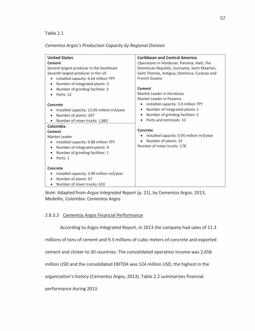
57
Table 2.1
Cementos Argos’s Production Capacity by Regional Division
United States Cement Second largest producer in the Southeast Seventh largest producer in the US
Installed capacity: 6.64 million TPY Number of integrated plants: 3 Number of grinding facilities: 3 Ports: 12
Concrete
Installed capacity: 13.09 million m3/year Number of plants: 307 Number of mixer trucks: 1,882
Caribbean and Central America Operations in Honduras, Panama, Haiti, the Dominican Republic, Suriname, Saint Maarten, Saint Thomas, Antigua, Dominica, Curacao and French Guiana Cement Market Leader in Honduras Market Leader in Panama
Installed capacity: 3.8 million TPY Number of integrated plants: 1 Number of grinding facilities: 5 Ports and terminals: 10
Concrete
Installed capacity: 0.95 million m3/year Number of plants: 14
Number of mixer trucks: 178
Colombia Cement Market Leader
Installed capacity: 9.88 million TPY Number of integrated plants: 9 Number of grinding facilities: 1 Ports: 1
Concrete
Installed capacity: 3.99 million m3/year Number of plants: 67 Number of mixer trucks: 610
Note: Adapted from Argos Integrated Report (p. 21), by Cementos Argos, 2013, Medellin, Colombia: Cementos Argos
2.8.3.2 Cementos Argos Financial Performance
According to Argos Integrated Report, in 2013 the company had sales of 11.3
millions of tons of cement and 9.3 millions of cubic meters of concrete and exported
cement and clinker to 30 countries. The consolidated operation income was 2,656
million USD and the consolidated EBITDA was 524 million USD, the highest in the
organization’s history (Cementos Argos, 2013). Table 2.2 summarizes financial
performance during 2013.
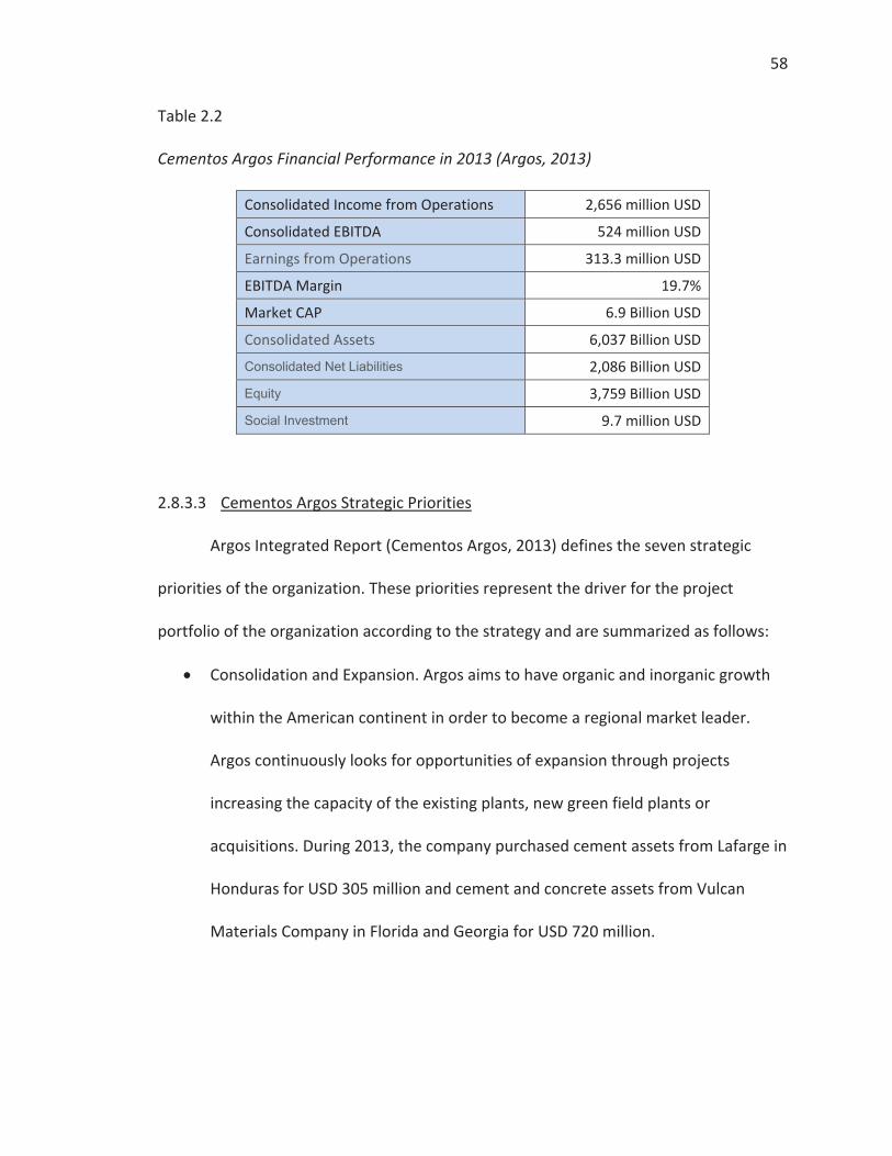
58
Table 2.2
Cementos Argos Financial Performance in 2013 (Argos, 2013)
Consolidated Income from Operations 2,656 million USD
Consolidated EBITDA 524 million USD
Earnings from Operations 313.3 million USD
EBITDA Margin 19.7%
Market CAP 6.9 Billion USD
Consolidated Assets 6,037 Billion USD Consolidated Net Liabilities 2,086 Billion USD Equity 3,759 Billion USD Social Investment 9.7 million USD
2.8.3.3 Cementos Argos Strategic Priorities
Argos Integrated Report (Cementos Argos, 2013) defines the seven strategic
priorities of the organization. These priorities represent the driver for the project
portfolio of the organization according to the strategy and are summarized as follows:
Consolidation and Expansion. Argos aims to have organic and inorganic growth
within the American continent in order to become a regional market leader.
Argos continuously looks for opportunities of expansion through projects
increasing the capacity of the existing plants, new green field plants or
acquisitions. During 2013, the company purchased cement assets from Lafarge in
Honduras for USD 305 million and cement and concrete assets from Vulcan
Materials Company in Florida and Georgia for USD 720 million.
59
Capital structure. With the purpose of levering its growth, Argos looks for the
availability of diverse sources of financial flexibility, keeping optimal levels of
long-term indebtedness. During 2013, the company raised USD 880 million
undertaking an issuance of shares with preferred dividend, both in domestic and
international markets. This represents a source of financial flexibility that can
support the growth of the organization.
Operational models. At the same time Argos is expanding the operations, the
company is working on the standardization and alignment of processes in order
to create synergies as a business group. During 2013, the Synergy Project allows
the company the standardization of the business core process and the
implementation of SAP platform in the Colombia and USA Regional Divisions
with an investment of USD 61.86 million.
Organizational excellence. Argos’s management model is based on excellence
which will make the organization more competitive and profitable. Argos is
promoting projects that increase operational efficiency and contribute to
decrease cost of production and distribution. This includes initiatives to lower
the clinker/cement factor, increase the run factor of the kilns, and reduce energy
consumption and the use of alternative fuels.
Innovation. Research and Development guarantee the continuous
transformation and reinvention of the company towards sustainable
competitiveness in the business world. Innovation in Argos is focused on four

60
lines: innovation management, new businesses, research and development and
the use of alternative resources. During 2013, income stemming from the sale of
innovating products reached a total of USD 252.9 million, which is 9.8% of the
total company income. Beside this, the company had USD 3.3 million saving
thanks to innovative ideas.
Strategic projects. Argos is undertaking important investments with emphasis on
improving the profitability and sustainability of the markets in which the
company operates. During 2013, the strategic projects in execution were the
expansion of capacity in three plants in Colombia in 900,000 tons of cement per
year with an investment of USD 120 million, a new distribution center in
Cartagena of 1 million tons of cement with an investment of USD 35 million and
the installation of a new cement mill at the Harleyville plant in the USA with a
capacity of 0.5 million tons of cement per year with an investment of USD 48
million.
Sustainability. Cementos Argos develops its operations managing impacts, risk,
and opportunities from the economic, social and environmental points of view.
As a result of this policy, the company was included in the Dow Jones
Sustainability Index (DJSI) in 2013, in the World category, as well as in that of
Emerging Markets. The DJSI is the first and most important index that measures
management in terms of sustainability. Argos is one of four cement companies
worldwide to be included in this index.

61
2.9 Summary
This chapter has provided an overview of methodologies for project selection,
including nonnumeric and numeric methods with more emphasis in optimization
methods using mathematical programming. An overview of commercial solutions for
portfolio project selection was also included and finally an introduction to Cementos
Argos and the case study of project selection that is discussed in detail in chapter 4.
62
CHAPTER 3. METHODOLOGY
The main goal of this research was to develop the formulation of a model and a
computational tool (Decision Support System) to assist decision makers in the process of
project portfolio selection. The model developed was based on a combination of
mathematical programming techniques. This research includes the mathematical
formulation of the model, the design and development of a computational tool for the
end user, the verification and validation of the DSS and, finally, the application of the
computational tool on a case study to evaluate its usefulness. This chapter presents the
framework for project selection, a description of the computational tool, the verification
and validation process, experimental design and analysis.
3.1 Portfolio Selection and Optimization Framework
Project selection tools should be used to support an integrated portfolio
selection process as a part of the portfolio management of the organization. A critical
successful factor in the implementation of a DSS for project selection is the adoption of
a basic framework. PMI (PMI, 2008b) presents a standard for portfolio management
described in Chapter 2. The main activities make it possible to identify, categorize,
evaluate, select, prioritize, and balance the portfolio.

63
Bible and Bivins (2011) developed a detailed Project Portfolio Management
(PPM) framework with a screening phase and a selection phase. In the screening phase
candidate projects are screened according to some criteria and the results of a business
case. The selection phase includes the evaluation of project benefits, followed by the
selection of initial portfolio and, finally, an optimization based on a ‘what if’ analysis.
Archer and Ghasemzadeh (1999) proposed a general framework for project
selection considering the entire project lifecycle from conception to closing phase. This
research adopts this framework with some modifications such as the inclusion of
reviewing for alignment with strategy in the pre-screening stage and reviewing for
feasibility according economical, technical and sustainability criteria in the screening
stage. Figure 3.1 shows this framework and the main stages are described as follows:
Candidate projects definitions. During this stage, a set of candidate projects are
proposed. These initiatives can come from customer requirements, market
opportunity, legal/environmental requirement, new technology available,
research and development of new products or process, etc.
Pre-Screening Stage. During this stage, candidate projects are reviewed if they
are linked to at least one strategic goal of the organization. Any project that
does not meet this criterion should be eliminated from the selection process in
this stage.

64
Figure 3.1 .Framework for Project Portfolio Selection. Adapted from “An integrated framework for project portfolio selection” by Archer, N., & Ghasemzadeh, F., 1999. International Journal of Project Management, 17(4), 207–216
Aligned with strategy?
Business Case Development for each
project
Economically feasible?
Economically feasible?
Pre-Screening Stage
Screening Stage
Yes
Yes
Exclude Candidate Project-
Update database
No
Project Study Stage
Feasibility Study
Candidate Projects
Potential projects definition
Sustainable?
Technically feasible?
Optimal Portfolio
Project Selection
Portfolio Adjustment
Project/Portfolio Execution
Project/Portfolio Performance Assessment
Yes
Selection Stage
Project Selection
Portfolio Adjustment
Execution Stage
Closing Stage
Update database
Yes
No No No
Define: Objectives, resources availability,
time horizon
Yes
65
Project Study. This stage has as a goal developing a business case of potential
projects with the purpose of defining some main attributes of the projects such
as NPV, costs, demand of technical and human resources, duration and risk level.
Screening Stage. This stage considers the assessment of different criteria that are
critical success factors for any project and includes economic and technical
feasibility and sustainability assessment. The economic evaluation ensures the
project is profitable for the organization. Technical feasibility ensures the
organization can obtain the technology and resources to undertake the project.
The sustainability assessment includes environmental and social impact
considerations.
Selection Stage. This stage has two parts: project selection and portfolio
adjustment. The main purpose of this research is designing and implementing a
Decision Support System (DSS), based on mathematical programming techniques
which find the optimal set of projects that maximize the benefits subjected to
customized constraints (technical requirements, resources constraints and
interdependence among projects). After an optimal solution is found, the
decision making team has the possibility to make adjustments in the final
portfolio through a sensitivity analysis (e.g., including or excluding some
candidate projects or modifying the constraints).
Execution Stage. This stage includes the activities required to develop all
deliverables of the project according to scope, time and cost approved.
66
Closing Stage. This stage should include the assessment of project performance
and verification that the goals of the project were met. This stage gives valuable
information and learned lessons to the organization for future projects.
3.2 Project Portfolio Selection Model
This research focuses on developing a DSS to assist the decision makers during
the selection stage of the project portfolio selection process illustrated in Figure 3.1.
The project selection approach is based on mathematical programming and applies two
approaches according to the conditions of the problem:
1. 0-1 Integer linear programming (ILP) when the decision maker wants to
optimize one goal. For default, in this approach the objective function seeks to
maximize NPV, even though is possible to define other criterion of
optimization such as throughput or revenue. The corresponding mathematical
model was described in Section 2.6.1 of this document.
2. Weighted goal programming (GP) when the decision maker wants to satisfy
multiple goals. In this case, the decision maker will define its goals and targets.
These objectives should be linked to the strategic goals of the organization.
The relative importance of the goals (weights) may be defined by direct
assignation in case of one decision maker, or using a technique such as
analytical hierarchy process (AHP) or analytical network process (ANP) in the
67
case of a decision making team. The corresponding mathematical model for
this approach was presented in Section 2.6.2 of this document.
The DSS gives the possibility of project selection and scheduling considering the
availability of resources in the planning horizon, which results in two possibilities:
1. Project selection assuming all projects are undertaken at the same time and
with a defined amount of resources available for project execution. In this case
it is considered only one period of time.
2. Project selection considering a planning horizon for project execution and
availability of resources according to each period. In this case, the DSS finds the
best set of projects and the sequence of execution.
The DSS can incorporate the following kinds of constraints:
1. Available resources of the company to develop the portfolio, including financial
resources, manpower, production and logistic resources.
2. Technical requirements such as productivity level, specifications, risks, or
environmental requirements.
3. Project interdependence within the portfolio such as contingent projects,
mutually exclusive projects, mandatory and ongoing projects.
The complete formulation of the mathematical programming for all these models
are summarized in the Table 3.1 to Table 3.4. All the equations were described in
sections 2.6.1 and 2.6.2.
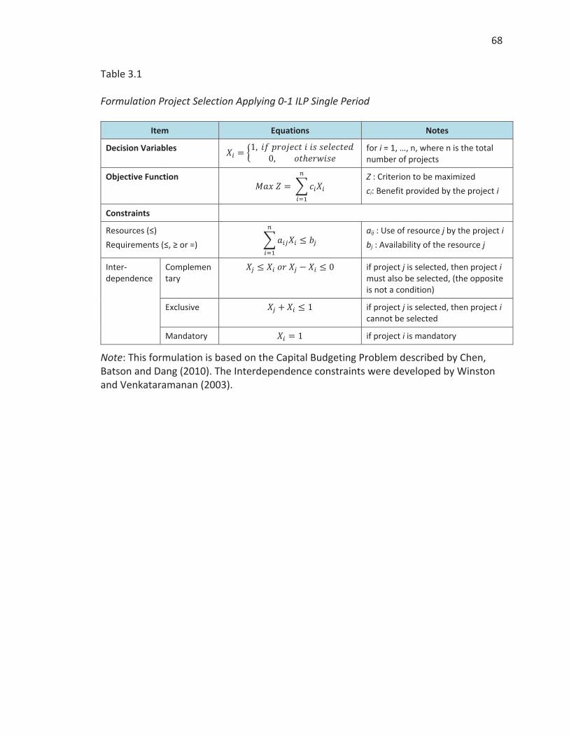
68
Table 3.1
Formulation Project Selection Applying 0-1 ILP Single Period
Item Equations Notes
Decision Variables for i = 1, …, n, where n is the total number of projects
Objective Function
Z : Criterion to be maximized ci: Benefit provided by the project i
Constraints
Resources (≤) Requirements (≤, ≥ or =)
aij : Use of resource j by the project i bj : Availability of the resource j
Inter-dependence
Complementary
if project j is selected, then project i must also be selected, (the opposite is not a condition)
Exclusive if project j is selected, then project i cannot be selected
Mandatory if project i is mandatory
Note: This formulation is based on the Capital Budgeting Problem described by Chen, Batson and Dang (2010). The Interdependence constraints were developed by Winston and Venkataramanan (2003).
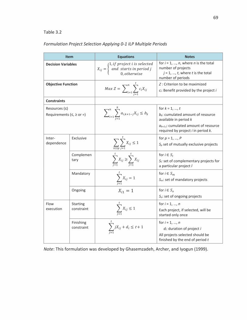
69
Table 3.2
Formulation Project Selection Applying 0-1 ILP Multiple Periods
Item Equations Notes
Decision Variables
for i = 1, …, n, where n is the total number of projects j = 1, …, t, where t is the total number of periods
Objective Function
Z : Criterion to be maximized ci: Benefit provided by the project i
Constraints
Resources (≤) Requirements (≤, ≥ or =)
for k = 1, …, t bk: cumulated amount of resource available in period k ak+1-j: cumulated amount of resource required by project i in period k.
Inter-dependence
Exclusive
for p = 1, …, P Sp set of mutually exclusive projects
Complementary
for i Sl: set of complementary projects for a particular project l
Mandatory
for i Sm: set of mandatory projects
Ongoing for i So: set of ongoing projects
Flow execution
Starting constraint
for i = 1, …, n Each project, if selected, will be started only once
Finishing constraint
for i = 1, …, n di: duration of project i All projects selected should be finished by the end of period t
Note: This formulation was developed by Ghasemzadeh, Archer, and Iyogun (1999).

70
Table 3.3
Formulation Project Selection Applying Weighted GP Single Period
Item Equations Notes
Decision Variables for i = 1, …, n, where n is the total number of projects
Objective Function
Qp
Z : total deviation of the any project set from the goals Qp :normalization const. of pth goal Sp :deviation of the pth goal
Constraints
Goal Constraints ppp
n
iipi gSeSuXc
1
Cpi : contribution to the pth goal by the project i gp : target of goal p
Resources (≤) Requirements (≤, ≥ or =)
aiq : Use of resource q by the project i bq : Availability of the resource q
Inter-dependence
Complementary
if project j is selected, then project i must also be selected, (the opposite is not a condition)
Exclusive if project j is selected, then project i cannot be selected
Mandatory if project i is mandatory
Note: This formulation was developed by the author. The Interdependence constraints were developed by Winston and Venkataramanan (2003).
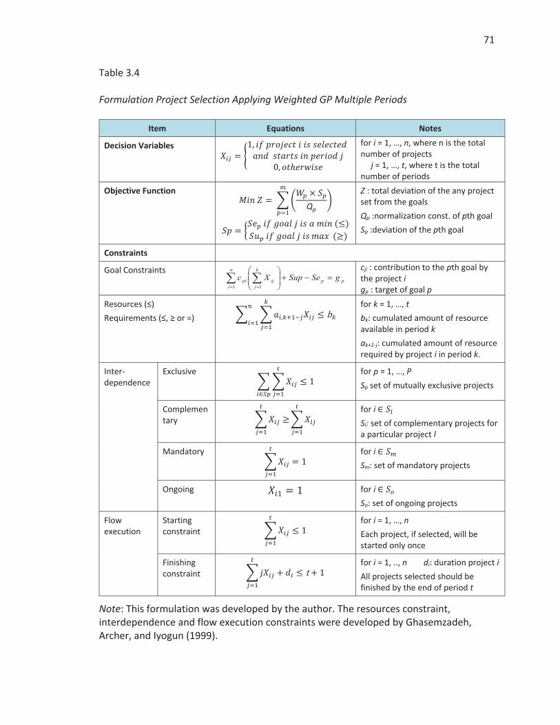
71
Table 3.4
Formulation Project Selection Applying Weighted GP Multiple Periods
Item Equations Notes
Decision Variables
for i = 1, …, n, where n is the total number of projects j = 1, …, t, where t is the total number of periods
Objective Function
Qp
Z : total deviation of the any project set from the goals Qp :normalization const. of pth goal Sp :deviation of the pth goal
Constraints
Goal Constraints pp
k
jij
n
ipi gSeSupXc
11
cji : contribution to the pth goal by the project i gp : target of goal p
Resources (≤) Requirements (≤, ≥ or =)
for k = 1, …, t bk: cumulated amount of resource available in period k ak+1-j: cumulated amount of resource required by project i in period k.
Inter-dependence
Exclusive
for p = 1, …, P Sp set of mutually exclusive projects
Complementary
for i Sl: set of complementary projects for a particular project l
Mandatory
for i Sm: set of mandatory projects
Ongoing for i So: set of ongoing projects
Flow execution
Starting constraint
for i = 1, …, n Each project, if selected, will be started only once
Finishing constraint
for i = 1, .., n di: duration project i All projects selected should be finished by the end of period t
Note: This formulation was developed by the author. The resources constraint, interdependence and flow execution constraints were developed by Ghasemzadeh, Archer, and Iyogun (1999).
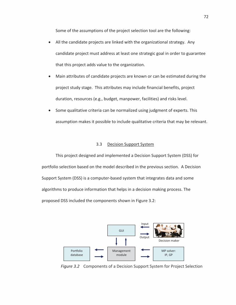
72
Some of the assumptions of the project selection tool are the following:
All the candidate projects are linked with the organizational strategy. Any
candidate project must address at least one strategic goal in order to guarantee
that this project adds value to the organization.
Main attributes of candidate projects are known or can be estimated during the
project study stage. This attributes may include financial benefits, project
duration, resources (e.g., budget, manpower, facilities) and risks level.
Some qualitative criteria can be normalized using judgment of experts. This
assumption makes it possible to include qualitative criteria that may be relevant.
3.3 Decision Support System
This project designed and implemented a Decision Support System (DSS) for
portfolio selection based on the model described in the previous section. A Decision
Support System (DSS) is a computer-based system that integrates data and some
algorithms to produce information that helps in a decision making process. The
proposed DSS included the components shown in Figure 3.2:
Figure 3.2 Components of a Decision Support System for Project Selection
Input
GUI
Portfolio database
MP solver: IP, GP
Management module
Decision maker Output

73
Mathematical programming (MP) solver which applies the algorithms to solve
the optimization problem.
Project portfolio database that keeps all the information of the candidate and
selected projects.
Graphical user interface (GUI) that allows the decision maker to interact with the
system.
Management module that addresses the flow of data and information between
the different components of the system
The proposed DSS provides the following information to the decision makers:
The set of projects that maximize the benefit (objective function) meeting all the
constraints (one objective problem).
The set of projects that satisfy the target goals meeting all the constraints
(multiple-objective problem).
Sequence of project execution (scheduling) in case of defining a planning
horizon.
The DSS can be customized according to the needs of the organization, policies
regarding resources allocation, and portfolio management. This tool does not replace
knowledge and experience of experts, but provides insights for the decision making
team.

74
3.4 Modeling Language Selection
As described in section 2.6.3, developing a decision support system requires the
use of a modeling language and solvers. The following commercial software tools were
considered in this research: AIMMS, AMPL, LINGO, MPL and Solver SDK Platform. All
these programming languages have incorporated solvers of last generation for LP, IP
and MIP and are very popular in the academia. The following paragraphs briefly
describe the programming languages considered in this research.
AIMMS, which stands for “Advanced Interactive Multidimensional Modeling
System" is an integrated optimization modeling language developed by Paragon
Decision Technology in 1993. It consists of an algebraic modeling language and
an integrated development environment for creating optimization models and
their corresponding graphical user interfaces. AIMMS support a wide range of
optimization models including linear, nonlinear, mixed Integer, stochastic
programming and robust optimization. AIMMS incorporates multiple solvers
including CPLEX, Gurobi, MOSEK and KNITRO. It also facilitates the use of
external data sources such as spreadsheets, databases, XML and text files
(Roelofs & Bisschop, 2013).
AMPL, which stands for “A Mathematical Programming Language" is a powerful
and one of the most popular modeling languages for linear and nonlinear
optimization problems, in discrete or continuous variables. AMPL was
developed by Bell Laboratories in 1985 and supports many solvers, both open

75
source and commercial, including CPLEX, Gurobi, and KNITRO. AMPL is available
for 32 and 64-bit platforms including Linux, Mac OS X and Windows (Fourer, Gay,
& Kernighan, 2003).
LINGO is a Fortran-based optimization software designed by LINDO Systems, Inc.
in 1988. LINGO incorporates a presolver for model reformulation and all the
solvers (linear, integer, nonlinear, etc) are linked to its modeling environment in
such a way that LINGO automatically sends the model to the most suitable
solver. LINGO solves the LP problems using any variation of simplex algorithm
and IP problems using branch and bound algorithm. LINGO supports Windows
and UNIX and allows interfacing with some of the most used programming
languages such as Visual Basic, C/C++, Fortran and Visual Java (Chen, Batson &
Dang, 2010).
MPL, which stands for “Mathematical Programming Language”, is produced by
Maximal Software, Inc. MPL can be used with many commercial and open
source solvers. MPL has a friendly graphical user interface in Windows and offers
an easy coding syntax similar to the algebraic language used in problem
formulation. Besides Windows, MPL supports UNIX and have a good interface
with spreadsheets and databases (Chen, Batson & Dang, 2010).
Solver SDK Platform is a comprehensive software development kit created by
Frontline Solvers, the developers of the Excel Solver add-in application, and
allows creating custom applications for optimization and Monte Carlo simulation

76
using languages such as Visual basic, C/C++, Java and Matlab. Solver SDK
supports Windows and Linux and allows integration with other Windows
applications such as Microsoft Excel.
Table 3.5 describes the most relevant criteria considered by the author for
selecting the programming language. The criteria considered are the following:
Software type: This criterion makes reference to whether the programming
language is integrated with solvers or not. It is more convenient have a
programming language that is integrated with solvers.
Platform: Operating system that supports the programming language. It is
desirable that the software can run under windows because this is a broadly
used operating system.
Academic License: This criterion refers to the cost of the license for academic
purposes.
Data compatibility: capacity of import and export data from different sources. It
is desirable that the software has at least the capacity of importing and
exporting data to Excel because many companies use spreadsheets to storage
and analyze data.
Variable types: This criterion refers to the nature of the variables that the
software can handle. The problems related to project selection correspond to
Integer Linear Programming (ILP) and Mixed Integer Linear Programming (MILP),
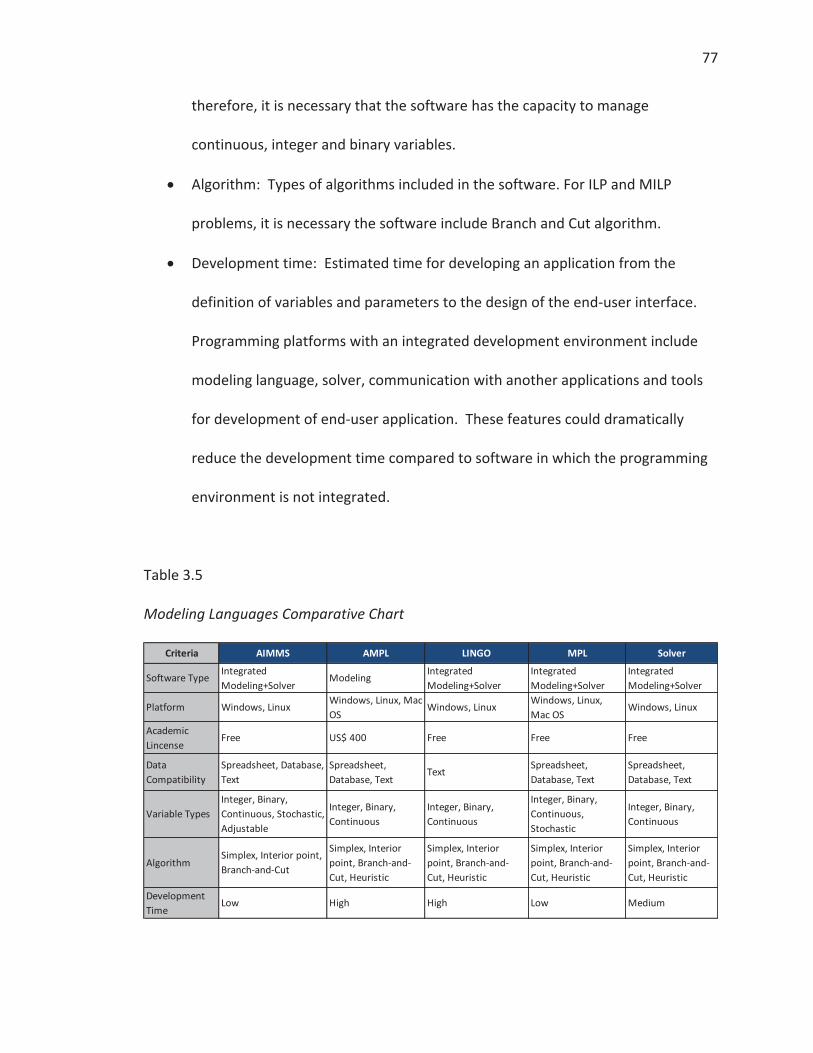
77
therefore, it is necessary that the software has the capacity to manage
continuous, integer and binary variables.
Algorithm: Types of algorithms included in the software. For ILP and MILP
problems, it is necessary the software include Branch and Cut algorithm.
Development time: Estimated time for developing an application from the
definition of variables and parameters to the design of the end-user interface.
Programming platforms with an integrated development environment include
modeling language, solver, communication with another applications and tools
for development of end-user application. These features could dramatically
reduce the development time compared to software in which the programming
environment is not integrated.
Table 3.5
Modeling Languages Comparative Chart
Criteria AIMMS AMPL LINGO MPL Solver
Software Type Integrated Modeling+Solver
Modeling Integrated Modeling+Solver
Integrated Modeling+Solver
Integrated Modeling+Solver
Platform Windows, Linux Windows, Linux, Mac OS
Windows, Linux Windows, Linux, Mac OS
Windows, Linux
Academic Lincense
Free US$ 400 Free Free Free
Data Compatibility
Spreadsheet, Database, Text
Spreadsheet, Database, Text
Text Spreadsheet, Database, Text
Spreadsheet, Database, Text
Variable TypesInteger, Binary, Continuous, Stochastic, Adjustable
Integer, Binary, Continuous
Integer, Binary, Continuous
Integer, Binary, Continuous, Stochastic
Integer, Binary, Continuous
AlgorithmSimplex, Interior point, Branch-and-Cut
Simplex, Interior point, Branch-and-Cut, Heuristic
Simplex, Interior point, Branch-and-Cut, Heuristic
Simplex, Interior point, Branch-and-Cut, Heuristic
Simplex, Interior point, Branch-and-Cut, Heuristic
Development Time
Low High High Low Medium
78
After review the features of all of this platforms, AIMMS was chosen for this
research due to the following reasons:
1. AIMMS is an optimization development environment which offers the state
of the art in algorithms, solvers and connectivity with external data and
applications. The last update of AIMMS is 3.13 released in 2013.
2. AIMMS modeling language includes a powerful combination of
multidimensional definitions and procedural execution and a rich set of
mathematical, statistical and financial functions.
3. AIMMS includes modeling language, preprocessor, world class solvers (e.g.,
CPLEX, Gurobi and CONOPT) and a tool for constructing a custom graphical
user interface (GUI) for a particular application.
4. AIMMS can deal with many kinds of optimization problems including linear
programming (LP), integer programming (IP), mixed integer programming
(MIP), quadratic programming (QP), nonlinear programming (NLP), stochastic
programming and robust optimization.
5. AIMMS academic version is free and totally functional.
6. Paragon technology has many information resources about AIMMS including
manuals, tutorials, examples and online workshops.
7. AIMMS offers connectivity with external data, spreadsheets and databases
using ODBC or OLE DB.

79
8. AIMMS support linkages to other applications using Application
Programming Interface (API) as well as Component Object Model (COM)
interface.
9. Finally, the development time in AIMMS could be less than the time required
in other platforms because AIMMS is an integrated development software
which includes a graphical programming environment with many toolbars
that facilitate the coding and debugging process, the communication with
other software (spreadsheet and database) and the development of the end-
user interface.
AIMMS include solvers for Linear Programming (LP), Mixed Integer Programming
(MIP), Nonlinear Programming (NLP), Quadratic Programming (QP), Quadratically
Constrained Programming (QCP), Mixed Integer Quadratic Programming (MIQP), Mixed
Integer Quadratically Constrained Programming (MIQCP), Mixed Complementary
Problems (MCP), Mathematical Programs with Complementarity Constraints (MPCC)
and Mixed Integer Nonlinear Programming (MINLP). The Figure 3.3 shows a screenshot
of the AIMMS solver configuration, which indicates the solvers included and the type of
associated problems.

80
Figure 3.3 . Screenshot of the Solver Configuration Page in AIMMS
The project portfolio selection problem corresponds to a Mixed Integer
Programming Problem, for these types of problems, AIMMS uses by default CPLEX as
solver. The other options are BARON, CBC, Gurobi, MOSEK and XA. The programmer can
select the solver to be used by AIMMS.
3.5 DSS Development
The development of the computational tool for project portfolio selection
required the following steps:
1. Definition of the problem. The needs and requirements of the decision makers
were studied by analyzing the type of criteria considered, objectives, constraints,
assumptions and the kind of information required as output to support the
decision making process.
2. Model construction (mathematical model). This step translates the real world
problem and creates (or select) a mathematical formulation that includes
81
functions, equations and inequalities that describe the objective function and
constraints. This step also verifies that all the assumptions for Mixed Integer
Programming (MIP) are satisfied. These assumptions are described in Chen,
Batson and Dang (2010) and summarized as follows:
Divisibility: All continuous variables are real numbers.
Integrality: All integer variables are integer or binary (0 or 1) numbers.
Certainty: All the parameters can be estimated and are constant
Proportionality: All objective functions and constraints are linear
Additivity: all objective functions and constraints can be expressed as a sum
of several functions, each of them containing a single variable.
Single-objective: All problems can be expressed as a single-objective
function, including the goal programming case with multiple goals.
Simultaneousness: Any feasible solution must satisfy simultaneously all the
constraints.
3. Model coding. This step translates the mathematical formulation in a
computational code using the programming language AIMMS. This step includes
the following:
Definition of the set of decision variables and parameters with its attributes.
Definition of the objective function and the objective variable according to
the formulations shown in Tables 3.1 to 3.4
82
Definition of all the constraints with inequalities corresponding to the
formulations shown in Tables 3.1 to 3.4
Assembly of each type of mathematical programing (MP) considered in the
DSS. Each MP definition includes the objective variable, direction of
optimization (minimization of maximization) the set of decision variables, the
set of constraints and the solver to be used.
4. Development of Graphical User Interface (GUI). The GUI makes possible the
interaction of the end user with the DSS. The GUI considered input pages, where
the user can specify the data for the problem configuration, candidate projects,
objectives and constraints. The output pages show the solution of the problem
including information of the optimal portfolio, the objectives and the
constraints.
5. Creation of Reports. This step comprises the design of printable page templates
that contain all the relevant information of the solution.
6. Integration with Excel. In this step, the interfaces required to import and export
data to Excel are developed.
After the development process, the verification and validation process was
undertaken in order to ensure the DSS is running free of errors and producing an
accurate solution for each problem. The verification and validation processes are shown
in the following section.
83
3.6 DSS Verification and Validation
The development of any DSS needs a verification and validation process that
guarantee the model and its implementation in a software platform are reliable. The
usefulness of a DSS is based on the confidence the tool offers to the modeler and the
potential user provided by a verification and validation process. This section describes
the verification and validation process employed by the author during the development
of the DSS for Project Portfolio Selection.
3.6.1 DSS Verification
Verification is the process that ensures the model behaves as intended (Kelton,
Sadowski & Swets, 2010). In the context of software development, verification is
normally called debugging. In a logical order, verification precedes the validation
process.
Verification deals with problems regarding model formulation, logical and
programing errors. These errors can cause infeasible solutions or unexpected results.
Inefficiently formulated statements can also cause excessively high execution times.
The verification process is usually carried out simultaneously with the coding process, so
after each piece of code is introduced in the main program, the proper operation is
verified in each running test. Some problems can be easy to find and another ones not-
so-obvious. AIMMS, the software platform chosen by the author, offers some tools for
the verification process as follows:

84
The AIMMS debugger helps in finding the location of the source of error in
declaration of variables, constraints or statement in procedures in the model.
The AIMMS profiler helps to solve computational time issues locating the most
time consuming process.
The author conducted a verification process while the elements of the
mathematical programming were integrated to the model using the AIMMS debugger. A
performance check was also done by monitoring the execution time during the
validation test using the AIMMS profiler.
3.6.2 DSS Validation
After the model is free of logical and programming errors and the execution time
is reasonable for a determined problem size (number of decision variables and
constraints), a validation is conducted. According Robinson (2008) a “valid model is
sufficiently accurate for the purpose at hand”. In this case, the DSS should accurately
find the best solution, which is the optimal portfolio, considering the variables,
parameters and constraints defined by the user.
In order to validate the DSS, the logical procedure is solving a problem whose
solution can be known for other method and compare the answers. The author uses a
basic problem with some variations, with the purpose of testing the functionality of the
DSS with one and multiples goals, different resources or requirements constraints and
projects interdependence relationship.

85
For the validation process, a basic problem proposed by Winston and
Venkataramanan (2003) was adapted as shown below:
A small aerospace company is considering eight projects for the portfolio. These
projects are described below.
Project 1: Develop an automated test facility
Project 2: Barcode all company inventory and machinery
Project 3: Introduce a CAD/CAM system
Project 4: Buy a new lathe and deburring system
Project 5: Institute FMS (flexible manufacturing system)
Project 6: Install a LAN (local area network)
Project 7: Develop AIS (artificial intelligence simulation)
Project 8: Set up a TQM (total quality management)
Each project has been rated on five attributes: ROI, cost, productivity
improvement, worker requirements, and degree of technological risk. These
ratings are given in the table below
Proj 1 Proj 2 Proj 3 Proj 4 Proj 5 Proj 6 Proj 7 Proj 82,070 456 670 350 495 380 1,500 480
900 240 335 700 410 190 500 1603 2 2 0 1 0 3 2
18 18 27 36 42 6 48 243 2 4 1 1 0 2 3
PeopleRisks
GoalsROI ($)Cost ($)Productivity
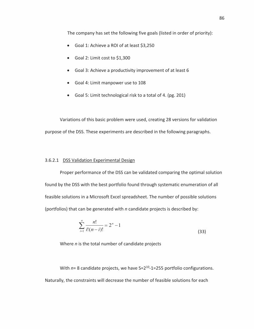
86
The company has set the following five goals (listed in order of priority):
Goal 1: Achieve a ROI of at least $3,250
Goal 2: Limit cost to $1,300
Goal 3: Achieve a productivity improvement of at least 6
Goal 4: Limit manpower use to 108
Goal 5: Limit technological risk to a total of 4. (pg. 201)
Variations of this basic problem were used, creating 28 versions for validation
purpose of the DSS. These experiments are described in the following paragraphs.
3.6.2.1 DSS Validation Experimental Design
Proper performance of the DSS can be validated comparing the optimal solution
found by the DSS with the best portfolio found through systematic enumeration of all
feasible solutions in a Microsoft Excel spreadsheet. The number of possible solutions
(portfolios) that can be generated with n candidate projects is described by:
12)!(!
!1
nn
i inin
(33)
Where n is the total number of candidate projects
With n= 8 candidate projects, we have S=210-1=255 portfolio configurations.
Naturally, the constraints will decrease the number of feasible solutions for each
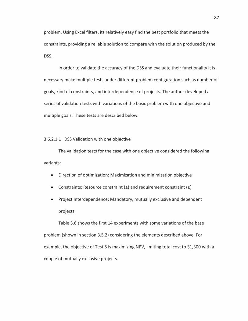
87
problem. Using Excel filters, its relatively easy find the best portfolio that meets the
constraints, providing a reliable solution to compare with the solution produced by the
DSS.
In order to validate the accuracy of the DSS and evaluate their functionality it is
necessary make multiple tests under different problem configuration such as number of
goals, kind of constraints, and interdependence of projects. The author developed a
series of validation tests with variations of the basic problem with one objective and
multiple goals. These tests are described below.
3.6.2.1.1 DSS Validation with one objective
The validation tests for the case with one objective considered the following
variants:
Direction of optimization: Maximization and minimization objective
Constraints: Resource constraint (≤) and requirement constraint (≥)
Project Interdependence: Mandatory, mutually exclusive and dependent
projects
Table 3.6 shows the first 14 experiments with some variations of the base
problem (shown in section 3.5.2) considering the elements described above. For
example, the objective of Test 5 is maximizing NPV, limiting total cost to $1,300 with a
couple of mutually exclusive projects.
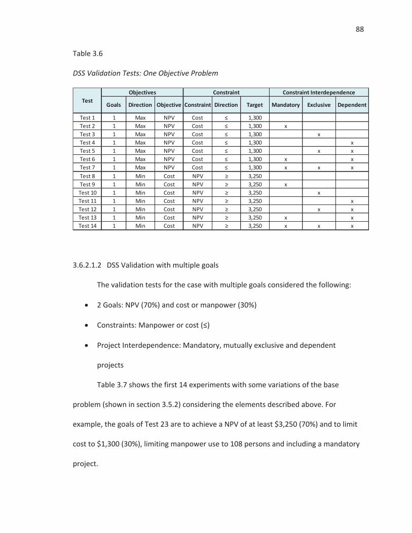
88
Table 3.6
DSS Validation Tests: One Objective Problem
3.6.2.1.2 DSS Validation with multiple goals
The validation tests for the case with multiple goals considered the following:
2 Goals: NPV (70%) and cost or manpower (30%)
Constraints: Manpower or cost (≤)
Project Interdependence: Mandatory, mutually exclusive and dependent
projects
Table 3.7 shows the first 14 experiments with some variations of the base
problem (shown in section 3.5.2) considering the elements described above. For
example, the goals of Test 23 are to achieve a NPV of at least $3,250 (70%) and to limit
cost to $1,300 (30%), limiting manpower use to 108 persons and including a mandatory
project.
Goals Direction Objective Constraint Direction Target Mandatory Exclusive Dependent
Test 1 1 Max NPV Cost ≤ 1,300Test 2 1 Max NPV Cost ≤ 1,300 xTest 3 1 Max NPV Cost ≤ 1,300 xTest 4 1 Max NPV Cost ≤ 1,300 xTest 5 1 Max NPV Cost ≤ 1,300 x xTest 6 1 Max NPV Cost ≤ 1,300 x xTest 7 1 Max NPV Cost ≤ 1,300 x x xTest 8 1 Min Cost NPV ≥ 3,250Test 9 1 Min Cost NPV ≥ 3,250 xTest 10 1 Min Cost NPV ≥ 3,250 xTest 11 1 Min Cost NPV ≥ 3,250 xTest 12 1 Min Cost NPV ≥ 3,250 x xTest 13 1 Min Cost NPV ≥ 3,250 x xTest 14 1 Min Cost NPV ≥ 3,250 x x x
Constraint Test
Objectives Constraint Interdependence
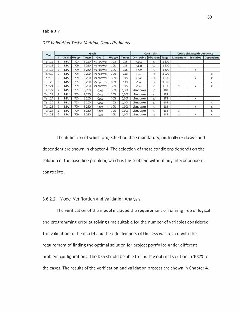
89
Table 3.7
DSS Validation Tests: Multiple Goals Problems
The definition of which projects should be mandatory, mutually exclusive and
dependent are shown in chapter 4. The selection of these conditions depends on the
solution of the base-line problem, which is the problem without any interdependent
constraints.
3.6.2.2 Model Verification and Validation Analysis
The verification of the model included the requirement of running free of logical
and programming error at solving time suitable for the number of variables considered.
The validation of the model and the effectiveness of the DSS was tested with the
requirement of finding the optimal solution for project portfolios under different
problem configurations. The DSS should be able to find the optimal solution in 100% of
the cases. The results of the verification and validation process are shown in Chapter 4.
# Goal 1 Weight Target Goal 2 Weight Target Constraint Direction Target Mandatory Exclusive DependentTest 15 2 NPV 70% 3,250 Manpower 30% 108 Cost ≤ 1,300Test 16 2 NPV 70% 3,250 Manpower 30% 108 Cost ≤ 1,300 xTest 17 2 NPV 70% 3,250 Manpower 30% 108 Cost ≤ 1,300 xTest 18 2 NPV 70% 3,250 Manpower 30% 108 Cost ≤ 1,300 xTest 19 2 NPV 70% 3,250 Manpower 30% 108 Cost ≤ 1,300 x xTest 20 2 NPV 70% 3,250 Manpower 30% 108 Cost ≤ 1,300 x xTest 21 2 NPV 70% 3,250 Manpower 30% 108 Cost ≤ 1,300 x x xTest 22 2 NPV 70% 3,250 Cost 30% 1,300 Manpower ≤ 108Test 23 2 NPV 70% 3,250 Cost 30% 1,300 Manpower ≤ 108 xTest 24 2 NPV 70% 3,250 Cost 30% 1,300 Manpower ≤ 108 xTest 25 2 NPV 70% 3,250 Cost 30% 1,300 Manpower ≤ 108 xTest 26 2 NPV 70% 3,250 Cost 30% 1,300 Manpower ≤ 108 x xTest 27 2 NPV 70% 3,250 Cost 30% 1,300 Manpower ≤ 108 x xTest 28 2 NPV 70% 3,250 Cost 30% 1,300 Manpower ≤ 108 x x x
Constraint Test Goals Constraint Interdependence

90
3.7 Case Study: Project Portfolio Selection in Cementos Argos - Metodology
This research includes the application of the DSS in a case of project selection in
Cementos Argos. The purpose of this case study is to evaluate the performance of the
DSS with real data, the information that the tool can provide for decision making and
explore the type of analysis that can be done. This case study have two parts as follows:
1. Project Portfolio Selection in Cementos Argos, 2006. In 2006, the company
evaluated 17 candidate projects for its portfolio using a weighted scoring model
based on financial criteria (NPV, IRR, PI and Payback). This case study is a
retrospective analysis which evaluated the potential improvement in the quality
of the proposed portfolio found using the DSS based on optimization vs. the
portfolio defined using the scoring model. A sensitivity analysis for the optimal
portfolios for different levels of budget constraint is included.
2. Project Portfolio Selection in Cementos Argos, 2014. In 2014, the company
considered 102 candidate projects for its portfolio. This case study is a
prospective analysis which found the best portfolio using the DSS considering
two approaches, the first is a global optimization considering all the projects
compete for the resources (budget constraint) vs a local optimization where the
projects compete for the resources in each regional division (the Caribbean, USA
and Colombia). The analysis shows the difference in terms of the distribution of
the portfolio per region, total benefit (NPN) and total cost of investment.
91
The development of the case study, results and analysis are shown in Chapter 4 of this
document.
3.8 Discussion
The project portfolio selection is basically a decision making process that should
be reasonable, accurate and unbiased. The selection problem may be complex when the
portfolio managers and top managers should considerer many candidate projects,
selection criteria, resources constraints and requirements. A DSS based on optimization
should have capacity and flexibility to find the best portfolio considering all this
elements.
The process of develop a DSS follows a general Operation Research modeling
process which comprises the following steps: review of the real world problem,
formulation of a mathematical model for the problem, coding of the model in a
programming language, verification or debugging process, validation of the
computational tool and, finally, the deployment of the DSS in the organization. An
important part of the process was the interaction with potential users (portfolio
managers and top managers) to define their information needs for making decisions
regarding the project selection process. The interaction with the potential users during
the deployment of the application was also important. Tests with real data and the
development of case studies as the case shown in this document allowed to make
adjustments to the tool and engage the potential users with the use of the tool.
92
3.9 Summary
This chapter has provided an overview of a framework for project selection, a
summary of the formulation of the model based on mathematical programming, a
description of the components of the DSS and the description of the verification and
validation process. The results of the verification and validation and a case study of
project portfolio selection in Cementos Argos are discussed in detail in chapter 4.

93
CHAPTER 4. DEVELOPING OF A DECISION SUPPORT SYSTEM FOR PROJECT PORTFOLIO SELECCTION-ARGOS CASE STUDY
This chapter presents a summary of architecture, execution flow and
functionality of the DSS for portfolio project selection included in the scope of this
research, the verification and validation process and results, and a case study of
Cementos Argos. This Case Study includes a portfolio selection process with historical
data of 2006 compared with the standard selection method employed by the company
and an application of project selection for 2015 projects.
4.1 Decision Support System for Project Portfolio Selection (DSS)
The main purpose of a Decision Support System is to provide insights that allow
decision makers to analyze the best alternatives and reduce the risk associated in a
decision making process. A DSS for project portfolio selection provides the portfolio that
adds more value to the organization.
This section describes the design features considered for the development of the
project portfolio selection tool, the architecture of the DSS and the functionality
indicating its capabilities.
94
4.1.1 DSS Design Features
The following design features were considered during the development of the
Project Portfolio Selection tool:
Simplicity. In most organizations the project portfolio selection process is
developed for a decision making team involving project managers and top
management, however these persons usually are not familiar with operations
research and optimization techniques. This DSS should guide the user during the
mathematical programming formulation, solution and analysis of results. The
process should be straightforward and error-free for the user.
User friendly. A simple and intuitive Graphical User Interface (GUI) in a windows
environment can makes easier the flow of information between user and DSS for
data input and data output. The representation of the results in graphical mode
using charts like bubble charts and Gantt charts, helps to draw conclusions about
the suggested project portfolios. AIMMS, the programming language selected,
allows the development of a GUI in the same programing environment avoiding
the necessity of using a different developing software for the GUI.
Flexibility. The developed DSS for project selection should be flexible enough to
be used in diverse organizations with different strategic objectives, categories of
projects, resources constraints, requirements and policies regarding the
assignment of resources for capital projects. This flexibility was achieved
separating the data from the application using multidimensional sets, symbolic
95
parameters, indexed variables and constraints and control flow commands. The
user can configure the selection problem: one or multiple objectives, single or
multiple periods, resource constraints, requirements, and project
interdependence.
Connectivity. When the amount of data in a project selection case is large,
besides the capability of input data through the GUI, the tool should be able to
import data from spreadsheets, text files or databases. In the same way, transfer
the solution to a spreadsheet or database for further analysis and data storage is
important. The developed tool should read data from and write the results to
Microsoft Excel Spreadsheets. Besides, for future development, it is possible to
read and write data with Open Database Connectivity (ODBC) and Object Linking
and Embedding for Databases (OLE DB) compliant databases such as Microsoft
Access, Microsoft SQL Server and Oracle.
Scalability. A DSS should be developed considering future expansions of
functionality. This scalability is achieved with a modular architecture of the code
that makes possible the integration with future components. For example, the
constraint equations are grouped in a set, and it is possible to add new
constraints to the set to consider in the problem formulation. The developed DSS
can incorporate new project categories, types of constraints, and even stochastic
parameters and variables.
96
4.1.2 DSS Architecture
The DSS developed in this thesis, is a software that integrates components in
order to solve four kind of mathematical problems (MP) regarding project portfolio
selection. The DSS has a modular architecture that integrates common elements (for
example, the project input module) with certain elements according to the kind of
problems to solve. The general architecture is shown in Figure 4.1 and its main
components are described in the following sections.
4.1.2.1 Configuration Module
This module allows the user to define the project selection problem to solve,
including the number of objectives (one or multiple), and the number of periods (single
or multiple). This options leads to one of the four kinds of problem formulation.
Project portfolio selection with one objective and single time period. The
mathematical programing model corresponds to 0-1 Integer Linear Programming
and the mathematical formulation was summarized in the Table 3.1. In this case
the decision variables, objective function, and constraints do not consider the
time horizon.
Project portfolio selection with one objective and multiple time periods. The
mathematical programing model corresponds to a 0-1 Integer Linear
Programming and the formulation was summarized in the Table 3.2. In this case
the decision variables, objective function and constraints consider the time
97
horizon in order to find execution sequence of the selected projects (portfolio
roadmap).
Project portfolio selection with multiple goals and a single time period. The
mathematical programing model corresponds to Weighted Goal Programming
and the mathematical formulation was summarized in the Table 3.3. In this case
the decision variables, objective function and constraints do not consider the
time horizon.
Project portfolio selection with multiple goals and multiple time periods. The
mathematical programing model corresponds to Weighted Goal Programming
and the mathematical formulation was summarized in the Table 3.4. In this case
the decision variables, objective function and constraints consider the time
horizon in order to find an execution sequence of the selected projects (portfolio
roadmap).
4.1.2.2 Data Input Module
This module includes all the screens that allow the reception of data from the
user as follows:
Candidate projects. Relevant information in this section includes the number of
candidate projects, NPV, cost, risk, duration, and two project categories that can
be customized. Additional criteria can be included. This module allows importing
98
data from an Excel spreadsheet, which is helpful when the number of candidate
projects is large.
Objectives/Goals. This section includes the definition of objectives and direction
of the optimization (maximization or minimization) for one objective. In the case
of multiple goals, the relevant information comprises the criteria, weights and
targets. The direction in this case is always minimizing the total deviation of the
goals.
Constraints. This section allows the user to define constraints. The relevant
information consists of the defined criteria as resource or requirement, the
directions (≥ or ≤) and the thresholds or limits for the constraints.
Project Interdependence. This section allows the user to set some relationship
between candidate projects. Some projects can be mandatory, so they should be
included in the recommended portfolio. Others can form groups of mutually
exclusive projects and finally some projects can be dependent on others.
4.1.2.3 Mathematical Program Generator
This module assembles the mathematical program (MP) including the main
elements in its formulation: decision variables set, objective function with its direction
and the constraints set. The MP generator translates the algebraic language of the
formulation in a computer language and integrates it with user data.

99
Figure 4.1 . Architecture of the DSS for Project Portfolio Selection
Data Input
Configuration One Objective Single Period
One Objective Multiple Periods
Multiple Goals Single Period
Multiple Goals Multiple Periods
Objective/Goals
One Objective Criterion Maximize or Minimize
Multiple Objective Criteria, weight, target Minimize Deviation
Presolver/SolverType of MP: Mixed Integer Programming (MIP), Binary Integer Programming (BIP) Algorithm: Brach and Bound, Cutting Edge Plane Solver: CPLEX, GUROBI, BARON, etc
Constraints Resource/Requirement
Criteria Direction: ≥ or ≤ Threshold
Time dependent Resource/Requirement
Criteria, direction: ≥, ≤ Threshold per period
Project Interdependence Mandatory Projects Exclusive Projects Dependent Projects
Mathematical Program Generator Variables Set Objective function, Direction (Max or Min) Constraint Set
Data Output Project Portfolio Selected
Single Period Portfolio selected Portfolio’s NPV, Cost Bubble Chart
Multiple Periods Portfolio selected Portfolio cash flow Gantt chart
Constraints Contribution Resource/Requirement
Constraint compliance Project contribution to constraint
Objective/Goals Achievement
One Objective Obj. Achievement Project contribution to objective
Multiple ObjectiveDeviation of Goals (%) Project contribution to goals
Reports View Report Print Report Save report as .ps file
Candidate Projects
NPV, cost, risk, duration Parameters Categories: kind of projects, region, etc Import
Export to Excel Portfolio Objective/Goals achievement Constraint compliance Export
User
100
4.1.2.4 Presolver/Solver
AIMMS, as a modern algebraic modeling language, includes a presolver which
applies techniques to the original formulation with the purpose of get a formulation
easier to solve. Once the formulation is processed, the solver receives the model and a
specific set of data (instance of the problem), applies an algorithm and returns the
optimal solution. In the case of the DSS for project selection, the problem corresponds
to a pure binary integer programming (BIP) for one objective problem and mixed integer
programming (MIP) for multiple goals problem. AIMMS automatically selects the solver
that can solve these kinds of problems by applying an appropriate algorithm (branch
and bound, cutting edge plane, etc). AIMMS by default uses CPLEX, developed by IBM,
for this type of problems.
4.1.2.5 Data Output Module
This module includes all the screens that allow to display the solution of the MP
including the following elements:
Portfolio. The relevant information in this section includes the number of
selected projects and the total NPV, portfolio cost. A bubble chart depicts the
selected projects. In the case of a problem with multiple periods, a page shows a
Gantt chart with the portfolio roadmap in the planning horizon and the portfolio
cash flow in case cost is a time dependent constraint.

101
Objective/Goals Achievement. This section includes the optimal value of the
objective and the contribution of each project to this objective. In the case of
multiple goals, the weighted deviation of the goals (%), the estimated
achievement of each goal vs the target and the contribution of each project in
the portfolio to each goal.
Constraints. This section includes the expected value of each constraint vs the
threshold and the contribution of each project to each constraint.
4.1.2.6 Reports Module
This module allows the user to view, print and save (as a .ps file) the report
showing the solution information. The report includes the same information shown in
the data Output Module.
4.1.2.7 Export to Excel Module
This module allows exporting the results to an Excel spreadsheet. This is a very
useful feature for further information processing and analysis.
4.1.3 DSS Functionality
In the design of the DSS, the author considered elements in the formulation that
make possible to find the best project portfolio in diversity cases and problem
configurations. The functionality of the Decision Support System for project selection is

102
determined by the formulation employed, the parameters, variables and constraints.
Table 4.1 shows the main functionality features of the DSS designed by the author. A
tutorial for the use of the computational tool is included in the Appendix.
Table 4.1
Functionality of the DSS for Project Portfolio Selection
Category Element Features INPUT Projects Candidate projects n candidate projects
2 customizable projects categories Objective/Goals One Objective Maximization/Minimization
Multiple Goals Minimization deviation to targets Constraints Resources Any resource (Constraint type ≤)
Requirements Any requirement (Constraint type ≤ or ≥) Mandatory Projects Set of k mandatory projects Mutually exclusive Projects
l Sets of mutually exclusive projects
Dependent Projects m tuple of dependent projects Time dependent resources
Any resource dependent on time (Constraint type ≤)
OUTPUT Portfolio Selected projects Portfolio NPV, Cost, Risk
Bubble chart Portfolio Roadmap Gantt chart, cash flow
Objective/Goals Objective optimization Objective achievement Project contribution to objective
Goal satisfying % deviation of the goals Goals achievement Project contribution to goal
Constraint Resource Resource consumption Project´s resource consumption
Requirements Requirements achievement Project contribution to requirement
REPORTS/CONNECTIVITY Reports Solution Reports View, Save and Print Report Connectivity to spreadsheet
Excel input Project data input Excel output Portfolio, objectives and constraint
information
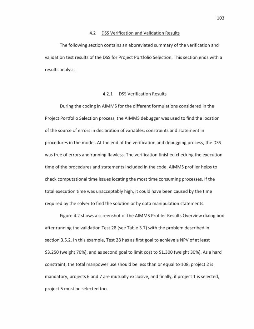
103
4.2 DSS Verification and Validation Results
The following section contains an abbreviated summary of the verification and
validation test results of the DSS for Project Portfolio Selection. This section ends with a
results analysis.
4.2.1 DSS Verification Results
During the coding in AIMMS for the different formulations considered in the
Project Portfolio Selection process, the AIMMS debugger was used to find the location
of the source of errors in declaration of variables, constraints and statement in
procedures in the model. At the end of the verification and debugging process, the DSS
was free of errors and running flawless. The verification finished checking the execution
time of the procedures and statements included in the code. AIMMS profiler helps to
check computational time issues locating the most time consuming processes. If the
total execution time was unacceptably high, it could have been caused by the time
required by the solver to find the solution or by data manipulation statements.
Figure 4.2 shows a screenshot of the AIMMS Profiler Results Overview dialog box
after running the validation Test 28 (see Table 3.7) with the problem described in
section 3.5.2. In this example, Test 28 has as first goal to achieve a NPV of at least
$3,250 (weight 70%), and as second goal to limit cost to $1,300 (weight 30%). As a hard
constraint, the total manpower use should be less than or equal to 108, project 2 is
mandatory, projects 6 and 7 are mutually exclusive, and finally, if project 1 is selected,
project 5 must be selected too.

104
Figure 4.2 . AIMMS Profiler Results Overview Screenshot after the Validation Test 28
Figure 4.3 . AIMMS Progress Window Screenshot after the Validation Test 28
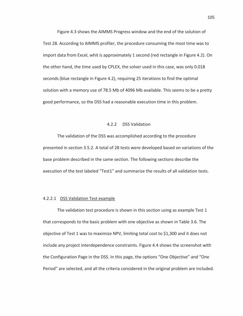
105
Figure 4.3 shows the AIMMS Progress window and the end of the solution of
Test 28. According to AIMMS profiler, the procedure consuming the most time was to
import data from Excel, whit is approximately 1 second (red rectangle in Figure 4.2). On
the other hand, the time used by CPLEX, the solver used in this case, was only 0.018
seconds (blue rectangle in Figure 4.2), requiring 25 iterations to find the optimal
solution with a memory use of 78.5 Mb of 4096 Mb available. This seems to be a pretty
good performance, so the DSS had a reasonable execution time in this problem.
4.2.2 DSS Validation
The validation of the DSS was accomplished according to the procedure
presented in section 3.5.2. A total of 28 tests were developed based on variations of the
base problem described in the same section. The following sections describe the
execution of the test labeled “Test1” and summarize the results of all validation tests.
4.2.2.1 DSS Validation Test example
The validation test procedure is shown in this section using as example Test 1
that corresponds to the basic problem with one objective as shown in Table 3.6. The
objective of Test 1 was to maximize NPV, limiting total cost to $1,300 and it does not
include any project interdependence constraints. Figure 4.4 shows the screenshot with
the Configuration Page in the DSS. In this page, the options “One Objective” and “One
Period” are selected, and all the criteria considered in the original problem are included.
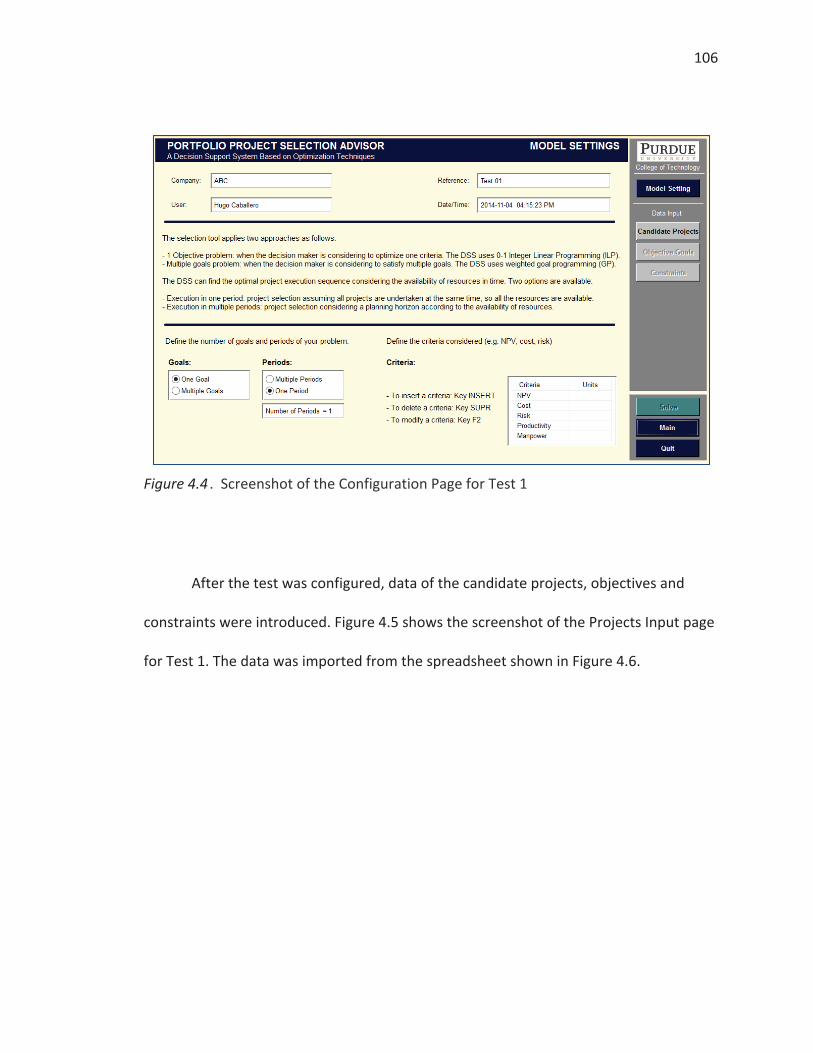
106
Figure 4.4 . Screenshot of the Configuration Page for Test 1
After the test was configured, data of the candidate projects, objectives and
constraints were introduced. Figure 4.5 shows the screenshot of the Projects Input page
for Test 1. The data was imported from the spreadsheet shown in Figure 4.6.

107
Figure 4.5 . Screenshot of the Projects Input Page for Test 1
Figure 4.6 . Screenshot of Excel Spreadsheet with Data for Test 1
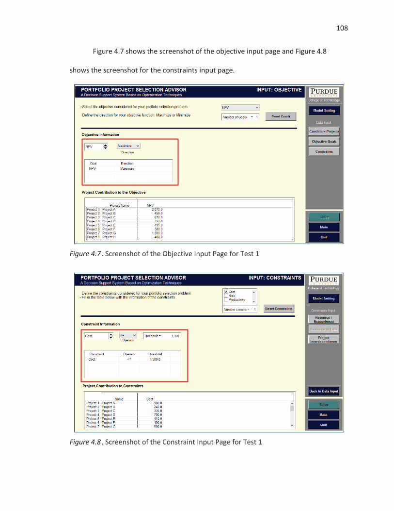
108
Figure 4.7 shows the screenshot of the objective input page and Figure 4.8
shows the screenshot for the constraints input page.
Figure 4.7 . Screenshot of the Objective Input Page for Test 1
Figure 4.8 . Screenshot of the Constraint Input Page for Test 1

109
After all the data are included, the optimal portfolio was found. Figure 4.9 shows
the screenshot of the Optimal Portfolio page. In the red rectangle are shown the
optimal portfolio which includes projects 2, 3, and 8. The maximal NPV achieved was
$3,106 and the total cost of the Portfolio was $1,235, which is lower than the budget
constraint of $1,300.
Figure 4.9 . Screenshot of the Solution Page for Test 1
In order to validate this result, the 255 project combinations (28-1 potential
portfolios) are listed on a spreadsheet. The optimal portfolio as shown in Figure 4.10, is
found by filtering the portfolios with a cost lower or equal to $1,300 and sorting the list
by decreasing NPV. It is also possible, to find the optimal solution using the Solver
function of Excel, indicating the objective cell, which contains NPV, the variables cells
(binary) and the constraint cells, which contains the cost, as shown in Figure 4.11.
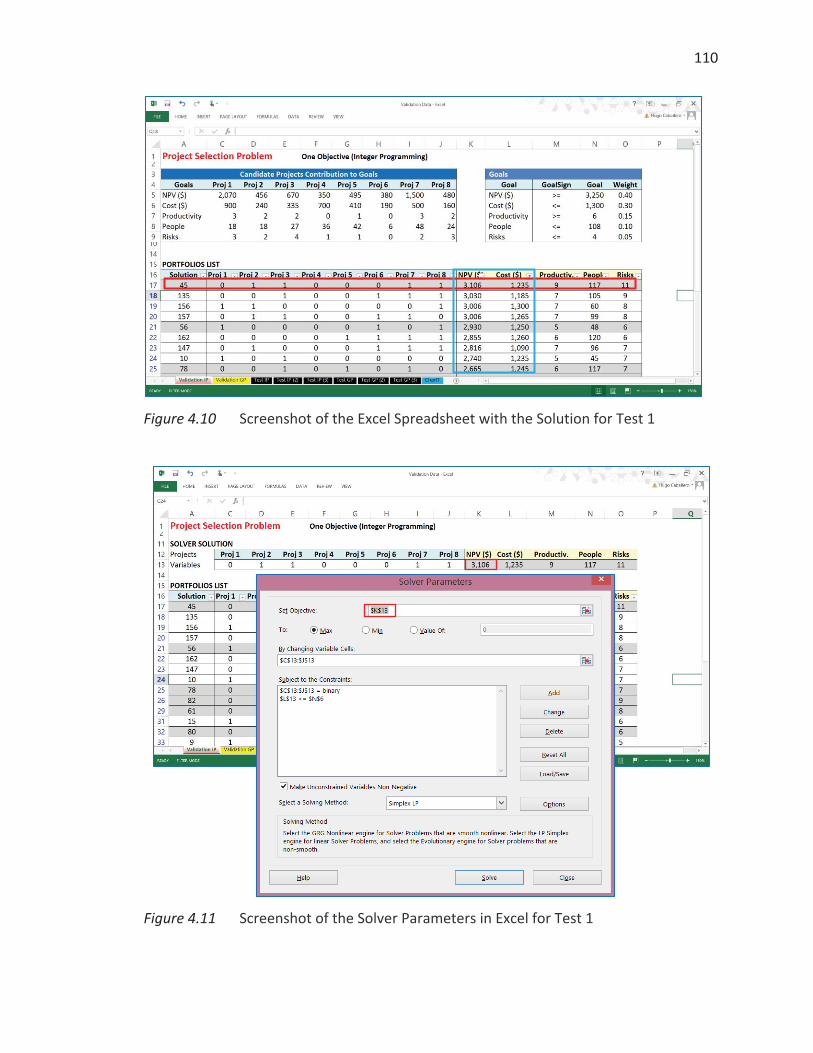
110
Figure 4.10 Screenshot of the Excel Spreadsheet with the Solution for Test 1
Figure 4.11 Screenshot of the Solver Parameters in Excel for Test 1
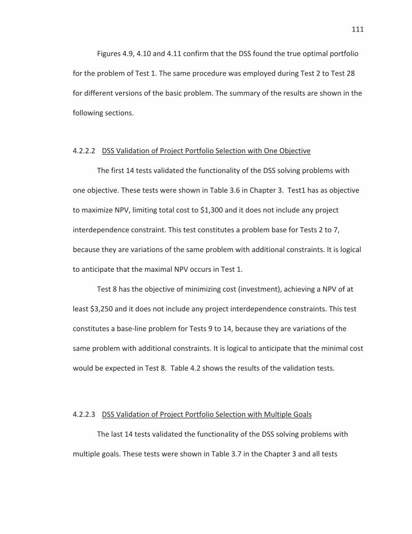
111
Figures 4.9, 4.10 and 4.11 confirm that the DSS found the true optimal portfolio
for the problem of Test 1. The same procedure was employed during Test 2 to Test 28
for different versions of the basic problem. The summary of the results are shown in the
following sections.
4.2.2.2 DSS Validation of Project Portfolio Selection with One Objective
The first 14 tests validated the functionality of the DSS solving problems with
one objective. These tests were shown in Table 3.6 in Chapter 3. Test1 has as objective
to maximize NPV, limiting total cost to $1,300 and it does not include any project
interdependence constraint. This test constitutes a problem base for Tests 2 to 7,
because they are variations of the same problem with additional constraints. It is logical
to anticipate that the maximal NPV occurs in Test 1.
Test 8 has the objective of minimizing cost (investment), achieving a NPV of at
least $3,250 and it does not include any project interdependence constraints. This test
constitutes a base-line problem for Tests 9 to 14, because they are variations of the
same problem with additional constraints. It is logical to anticipate that the minimal cost
would be expected in Test 8. Table 4.2 shows the results of the validation tests.
4.2.2.3 DSS Validation of Project Portfolio Selection with Multiple Goals
The last 14 tests validated the functionality of the DSS solving problems with
multiple goals. These tests were shown in Table 3.7 in the Chapter 3 and all tests
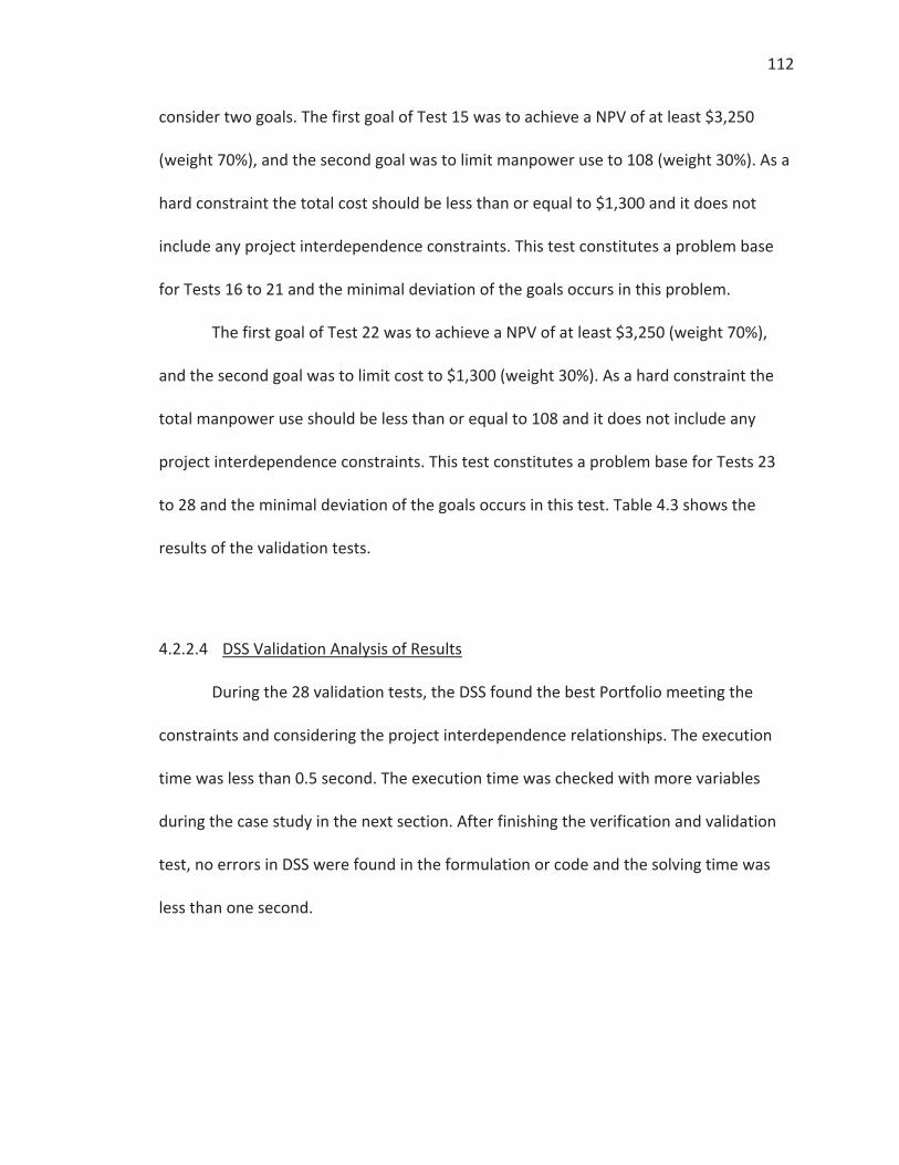
112
consider two goals. The first goal of Test 15 was to achieve a NPV of at least $3,250
(weight 70%), and the second goal was to limit manpower use to 108 (weight 30%). As a
hard constraint the total cost should be less than or equal to $1,300 and it does not
include any project interdependence constraints. This test constitutes a problem base
for Tests 16 to 21 and the minimal deviation of the goals occurs in this problem.
The first goal of Test 22 was to achieve a NPV of at least $3,250 (weight 70%),
and the second goal was to limit cost to $1,300 (weight 30%). As a hard constraint the
total manpower use should be less than or equal to 108 and it does not include any
project interdependence constraints. This test constitutes a problem base for Tests 23
to 28 and the minimal deviation of the goals occurs in this test. Table 4.3 shows the
results of the validation tests.
4.2.2.4 DSS Validation Analysis of Results
During the 28 validation tests, the DSS found the best Portfolio meeting the
constraints and considering the project interdependence relationships. The execution
time was less than 0.5 second. The execution time was checked with more variables
during the case study in the next section. After finishing the verification and validation
test, no errors in DSS were found in the formulation or code and the solving time was
less than one second.
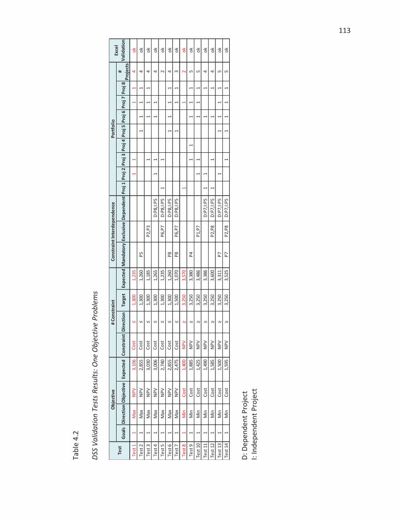
113
113
Tabl
e 4.
2
DSS
Valid
atio
n Te
sts R
esul
ts: O
ne O
bjec
tive
Prob
lem
s
D: D
epen
dent
Pro
ject
I:
Inde
pend
ent P
roje
ct
Goa
lsDi
rect
ion
Obj
ectiv
eEx
pect
edCo
nstr
aint
Dire
ctio
nTa
rget
Expe
cted
Man
dato
ryEx
clus
ive
Depe
nden
tPr
oj 1
Proj
2Pr
oj 3
Proj
4Pr
oj 5
Proj
6Pr
oj 7
Proj
8#
Proj
ects
Test
11
Max
NPV
3,10
6
Cost
≤1,
300
1,23
5
1
11
14
okTe
st 2
1M
axN
PV2,
855
Co
st≤
1,30
01,
260
P51
11
14
okTe
st 3
1M
axN
PV3,
030
Co
st≤
1,30
01,
185
P2,P
31
11
14
okTe
st 4
1M
axN
PV3,
006
Co
st≤
1,30
01,
265
D:P8
,I:P5
11
11
4ok
Test
51
Max
NPV
2,74
0
Cost
≤1,
300
1,23
5
P6
,P7
D:P8
,I:P5
11
2ok
Test
61
Max
NPV
2,85
5
Cost
≤1,
300
1,26
0
P8
D:P8
,I:P5
11
11
4ok
Test
71
Max
NPV
2,47
5
Cost
≤1,
500
1,07
0
P8
P6,P
7D:
P8,I:
P51
11
3ok
Test
81
Min
Cost
1,40
0
NPV
≥3,
250
3,57
0
1
12
okTe
st 9
1M
inCo
st1,
885
N
PV≥
3,25
03,
380
P41
11
11
5ok
Test
10
1M
inCo
st1,
425
N
PV≥
3,25
03,
486
P1,P
71
11
11
5ok
Test
11
1M
inCo
st1,
490
N
PV≥
3,25
03,
386
D:P7
,I:P5
11
11
4ok
Test
12
1M
inCo
st1,
585
N
PV≥
3,25
03,
600
P2,P
8D:
P7,I:
P51
11
14
okTe
st 1
31
Min
Cost
1,50
0
NPV
≥3,
250
3,31
1
P7
D:P7
,I:P5
11
11
15
okTe
st 1
41
Min
Cost
1,59
5
NPV
≥3,
250
3,52
5
P7
P2,P
8D:
P7,I:
P51
11
11
5ok
Cons
trai
nt In
terd
epen
denc
ePo
rtfo
lioO
bjec
tive
# Co
nstr
aint
Ex
cel
Valid
atio
nTe
st
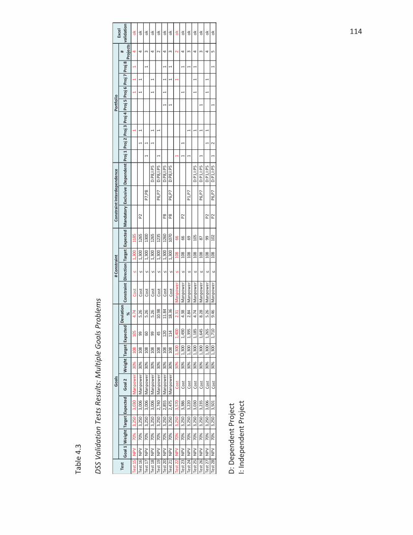
114
114
Tabl
e 4.
3
DSS
Valid
atio
n Te
sts R
esul
ts: M
ultip
le G
oals
Prob
lem
s
D: D
epen
dent
Pro
ject
I:
Inde
pend
ent P
roje
ct
Goa
l 1W
eigh
tTa
rget
Expe
cted
Goa
l 2W
eigh
tTa
rget
Expe
cted
Devi
atio
n%
Cons
trai
ntDi
rect
ion
Targ
etEx
pect
edM
anda
tory
Excl
usiv
eDe
pend
ent
Proj
1Pr
oj 2
Proj
3Pr
oj 4
Proj
5Pr
oj 6
Proj
7Pr
oj 8
# Pr
ojec
tsTe
st 1
5N
PV70
%3,
250
3,03
0M
anpo
wer
30%
108
105
4.74
Cost
≤1,
300
1185
11
11
4ok
Test
16
NPV
70%
3,25
03,
006
Man
pow
er30
%10
899
5.26
Cost
≤1,
300
1265
P21
11
14
okTe
st 1
7N
PV70
%3,
250
3,00
6M
anpo
wer
30%
108
605.
26Co
st≤
1,30
013
00P7
,P8
11
13
okTe
st 1
8N
PV70
%3,
250
3,00
6M
anpo
wer
30%
108
995.
26Co
st≤
1,30
012
65D:
P8,I:
P51
11
14
okTe
st 1
9N
PV70
%3,
250
2,74
0M
anpo
wer
30%
108
4510
.98
Cost
≤1,
300
1235
P6,P
7D:
P8,I:
P51
12
okTe
st 2
0N
PV70
%3,
250
2,85
5M
anpo
wer
30%
108
120
11.8
4Co
st≤
1,30
012
60P8
D:P8
,I:P5
11
11
4ok
Test
21
NPV
70%
3,25
02,
475
Man
pow
er30
%10
811
418
.36
Cost
≤1,
300
1070
P8P6
,P7
D:P8
,I:P5
11
13
okTe
st 2
2N
PV70
%3,
250
3,57
0Co
st30
%1,
300
1,40
02.
31M
anpo
wer
≤10
866
11
2ok
Test
23
NPV
70%
3,25
03,
386
Cost
30%
1,30
01,
490
4.38
Man
pow
er≤
108
66P2
11
11
4ok
Test
24
NPV
70%
3,25
03,
220
Cost
30%
1,30
01,
395
2.84
Man
pow
er≤
108
69P1
,P7
11
13
okTe
st 2
5N
PV70
%3,
250
3,03
0Co
st30
%1,
300
1,18
54.
74M
anpo
wer
≤10
810
5D:
P1,I:
P51
11
14
okTe
st 2
6N
PV70
%3,
250
3,23
5Co
st30
%1,
300
1,64
58.
28M
anpo
wer
≤10
887
P6,P
7D:
P1,I:
P51
11
3ok
Test
27
NPV
70%
3,25
03,
006
Cost
30%
1,30
01,
265
5.26
Man
pow
er≤
108
99P2
D:P1
,I:P5
11
11
4ok
Test
28
NPV
70%
3,25
03,
501
Cost
30%
1,30
01,
710
9.46
Man
pow
er≤
108
102
P2P6
,P7
D:P1
,I:P5
12
11
5ok
Cons
trai
nt In
terd
epen
denc
ePo
rtfo
lioG
oals
Exce
l va
lidat
ion
# Co
nstr
aint
Te
st
115
4.3 Case Study: Project Portfolio Selection in Cementos Argos – Results and Analysis
This section reviews the current portfolio selection process in Cementos Argos, a
retrospective analysis of the portfolio selection work in 2006 using the standard model
vs the information generated using the DSS and finally, a prospective of the portfolio
selection work for 2015 using the DSS.
4.3.1 Project Portfolio Selection Model in Cementos Argos
The selection of the projects for execution is an annual process in Cementos
Argos. The Financial planning department, which is part of the Financial Vice-presidency
(VP), is responsible for the evaluation and selection of the project portfolio of the
organization.
The process starts at the beginning of each year with the study of potential
projects in different Vice-presidencies and Regional Divisions (Colombia, Caribbean and
The USA). This business case study includes goals, scope, benefits, investment, financial
assessment and schedule. By the month of October, the Financial Planning Department
receives all the candidate projects from all VPs of the company. Currently, Financial
Planning Department considers only financial criteria and using a weighted scored
model for project portfolio selection. The criteria considered were Net Present Value
(NPV), Internal Rate of Return (IRR), Profitability Index (PI) and Payback period.
Candidate projects are scored in a scale from 0 to 5, where 5 is assigned to the
project with the best score for the criterion in consideration (e.g., 5 points to the project
116
with the highest NPV, 5 points to the project with the lowest Pay Back). The total score
for project i is found as was shown in Equation 6
(6)
Where wj is the weight of importance of the jth criterion
sij is the score of the project i for the jth criterion
4.3.2 Project Portfolio Selection in Cementos Argos in 2006
4.3.2.1 Project Portfolio Selection in Cementos Argos in 2006 with Scoring Weighted
Model
During 2006, the company considered 17 candidate projects for the cement,
concrete and logistics unit business to be executed during 2007. The projects comes
from Technical, Environmental, Concrete and Logistics VPs. The company provided a
business case for each of these projects and Table 4.4 summarizes their data. These
projects were then scored on a scale from 0 to 5, where 5 is assigned to the project with
the best score for the criteria considered. Table 4.5 shows the score for candidate
projects for each criterion. The projects in this table are sorted from best to worst
according to the score.

117
Table 4.4
Candidate Projects Considered by Cementos Argos in 2006
Table 4.5
Score of the Candidate Projects Considered by Cementos Argos in 2006
Project Name Category1 Category2 NPV Cost IRR PayBack PI[M USD] [M USD] [%] [Years] [%]
Project 1 Separator MC1 Tolu Technical Cement Colombia 5.4 1.2 83.0% 1.2 442%Project 2 Washing Plant Cartagena Concrete Concrete Colombia 3.3 0.3 84.0% 1.0 1188%Project 3 Power Plant Rioclaro Enviromental Cement Colombia 5.9 11.1 21.8% 6.0 53%Project 4 Pregrinding MC4 Cartagena Technical Cement Colombia 2.6 1.1 29.0% 2.5 239%Project 5 Dosifier Aditions Barranquilla Technical Cement Colombia 1.4 0.5 44.0% 2.0 286%Project 6 Kiln 5 Nare Technical Cement Colombia 3.7 12.0 16.2% 9.0 31%Project 7 Warehouse Rioclaro Logistics Cement Colombia 1.8 1.7 26.5% 4.0 108%Project 8 Power Plant Sogamoso Enviromental Cement Colombia 2.7 11.6 16.9% 7.0 23%Project 9 Port Cemas Logistics Cement Colombia 1.9 8.4 17.7% 6.0 23%Project 10 Crushing Plant El Carmen Concrete Concrete Colombia 1.0 0.4 24.9% 7.0 242%Project 11 Concrete Plant Bogota Concrete Concrete Colombia 0.5 0.9 20.5% 5.0 52%Project 12 Cement Silo Tolu Technical Cement Colombia 0.5 3.2 15.0% 5.0 15%Project 13 Coal Mine Trinidad Enviromental Cement Colombia 0.0 2.8 15.3% 7.0 0%Project 14 Crushing Plant Cairo Technical Cement Colombia -0.9 3.9 14.4% 10.0 0%Project 15 New Conveyors Logistics Logitrans -0.4 4.7 11.5% 50.0 0%Project 16 Warehouse Cairo Logistics Cement Colombia -0.4 1.0 6.6% 50.0 0%Project 17 Crushing Plant San Antonio Concrete Concrete Colombia -3.0 0.5 0.0% 50.0 0%TOTAL 65.2
Criterion 1: NPV NPV ScorePower Plant Rioclaro $5,921,702 5.0Separator MC1 Tolu $5,358,723 4.5Kiln 5 Nare $3,690,000 3.1Washing Plant Cartagena $3,267,867 2.8Power Plant Sogamoso $2,720,426 2.3Pregrinding MC4 Cartagena $2,637,872 2.2Port Cemas $1,914,630 1.6Warehouse Rioclaro $1,793,191 1.5Dosifier Aditions Barranquilla $1,447,826 1.2Crushing Plant El Carmen $1,049,565 0.9Cement Silo Tolu $488,936 0.4Concrete Plant Bogota $451,000 0.4Coal Mine Trinidad $11,299 0.0New Conveyors -$419,887 0.0Warehouse Cairo -$422,553 0.0Crushing Plant Cairo -$852,253 0.0Crushing Plant San Antonio -$2,992,609 0.0
Criterion 2: IRR IRR [%] ScoreWashing Plant Cartagena 84.0% 5.0Separator MC1 Tolu 83.0% 4.9Dosifier Aditions Barranquilla 44.0% 2.6Pregrinding MC4 Cartagena 29.0% 1.7Warehouse Rioclaro 26.5% 1.6Crushing Plant El Carmen 24.9% 1.5Power Plant Rioclaro 21.8% 1.3Concrete Plant Bogota 20.5% 1.2Port Cemas 17.7% 1.1Power Plant Sogamoso 16.9% 1.0Kiln 5 Nare 16.2% 1.0Coal Mine Trinidad 15.3% 0.9Cement Silo Tolu 15.0% 0.9Crushing Plant Cairo 14.4% 0.0New Conveyors 11.5% 0.0Warehouse Cairo 6.6% 0.0Crushing Plant San Antonio 0.0% 0.0
Criterion 3: Pay Back Pay Back ScoreWashing Plant Cartagena 1.00 5.0Separator MC1 Tolu 1.20 5.0Dosifier Aditions Barranquilla 2.00 5.0Pregrinding MC4 Cartagena 2.50 4.9Warehouse Rioclaro 4.00 4.9Concrete Plant Bogota 5.00 4.8Cement Silo Tolu 5.00 4.7Power Plant Rioclaro 6.00 4.6Port Cemas 6.00 4.5Crushing Plant El Carmen 7.00 4.3Power Plant Sogamoso 7.00 4.2Coal Mine Trinidad 7.00 4.1Kiln 5 Nare 9.00 3.9Crushing Plant Cairo 10.00 0.0New Conveyors 50.00 0.0Warehouse Cairo 50.00 0.0Crushing Plant San Antonio 50.00 0.0
Criterion 4: Profitability Index PI [%] ScoreWashing Plant Cartagena 1188% 5.0Separator MC1 Tolu 442% 1.9Dosifier Aditions Barranquilla 286% 1.2Crushing Plant El Carmen 242% 1.0Pregrinding MC4 Cartagena 239% 1.0Warehouse Rioclaro 108% 0.5Power Plant Rioclaro 53% 0.2Concrete Plant Bogota 52% 0.2Kiln 5 Nare 31% 0.1Power Plant Sogamoso 23% 0.1Port Cemas 23% 0.1Cement Silo Tolu 15% 0.1Coal Mine Trinidad 0% 0.0Crushing Plant Cairo 0% 0.0New Conveyors 0% 0.0Warehouse Cairo 0% 0.0Crushing Plant San Antonio 0% 0.0
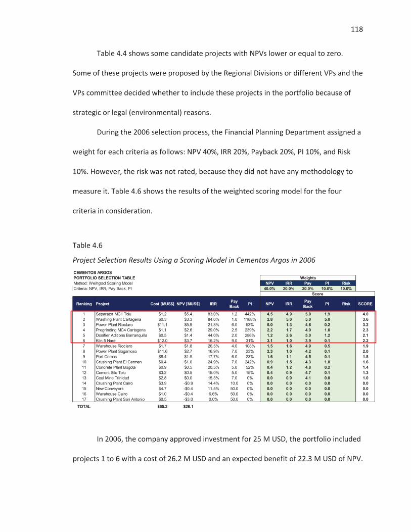
118
Table 4.4 shows some candidate projects with NPVs lower or equal to zero.
Some of these projects were proposed by the Regional Divisions or different VPs and the
VPs committee decided whether to include these projects in the portfolio because of
strategic or legal (environmental) reasons.
During the 2006 selection process, the Financial Planning Department assigned a
weight for each criteria as follows: NPV 40%, IRR 20%, Payback 20%, PI 10%, and Risk
10%. However, the risk was not rated, because they did not have any methodology to
measure it. Table 4.6 shows the results of the weighted scoring model for the four
criteria in consideration.
Table 4.6
Project Selection Results Using a Scoring Model in Cementos Argos in 2006
In 2006, the company approved investment for 25 M USD, the portfolio included
projects 1 to 6 with a cost of 26.2 M USD and an expected benefit of 22.3 M USD of NPV.
CEMENTOS ARGOSPORTFOLIO SELECTION TABLE WeightsMethod: Weihgted Scoring Model NPV IRR Pay PI RiskCriteria: NPV, IRR, Pay Back, PI 40.0% 20.0% 20.0% 10.0% 10.0%
Score
Ranking Project Cost [MUS$] NPV [MUS$] IRR Pay Back PI NPV IRR Pay
Back PI Risk SCORE
1 Separator MC1 Tolu $1.2 $5.4 83.0% 1.2 442% 4.5 4.9 5.0 1.9 4.02 Washing Plant Cartagena $0.3 $3.3 84.0% 1.0 1188% 2.8 5.0 5.0 5.0 3.63 Power Plant Rioclaro $11.1 $5.9 21.8% 6.0 53% 5.0 1.3 4.6 0.2 3.24 Pregrinding MC4 Cartagena $1.1 $2.6 29.0% 2.5 239% 2.2 1.7 4.9 1.0 2.35 Dosifier Aditions Barranquilla $0.5 $1.4 44.0% 2.0 286% 1.2 2.6 5.0 1.2 2.16 Kiln 5 Nare $12.0 $3.7 16.2% 9.0 31% 3.1 1.0 3.9 0.1 2.27 Warehouse Rioclaro $1.7 $1.8 26.5% 4.0 108% 1.5 1.6 4.9 0.5 1.98 Power Plant Sogamoso $11.6 $2.7 16.9% 7.0 23% 2.3 1.0 4.2 0.1 2.09 Port Cemas $8.4 $1.9 17.7% 6.0 23% 1.6 1.1 4.5 0.1 1.810 Crushing Plant El Carmen $0.4 $1.0 24.9% 7.0 242% 0.9 1.5 4.3 1.0 1.611 Concrete Plant Bogota $0.9 $0.5 20.5% 5.0 52% 0.4 1.2 4.8 0.2 1.412 Cement Silo Tolu $3.2 $0.5 15.0% 5.0 15% 0.4 0.9 4.7 0.1 1.313 Coal Mine Trinidad $2.8 $0.0 15.3% 7.0 0% 0.0 0.9 4.1 0.0 1.014 Crushing Plant Cairo $3.9 -$0.9 14.4% 10.0 0% 0.0 0.0 0.0 0.0 0.015 New Conveyors $4.7 -$0.4 11.5% 50.0 0% 0.0 0.0 0.0 0.0 0.016 Warehouse Cairo $1.0 -$0.4 6.6% 50.0 0% 0.0 0.0 0.0 0.0 0.017 Crushing Plant San Antonio $0.5 -$3.0 0.0% 50.0 0% 0.0 0.0 0.0 0.0 0.0
TOTAL $65.2 $26.1

119
4.3.2.2 Project Portfolio Selection in Cementos Argos in 2006 with the DSS Based on
Optimization
The DSS was used to find the optimal portfolio for Cementos Argos for the
planning year 2006 using the historical data shown in the Table 4.4 and considering the
following assumptions:
In order to simplify the analysis, the selection model considered one objective,
to maximize NPV, and a single period for the planning horizon.
The only resource constraint considered was the budget available of 25 M USD.
However, with the intention of demonstrating how to use the DSS, a sensitivity
analysis was run with the investment budget ranging from 10 to 65 M USD in
increments of 5 M USD.
Payback was considered in the model as a project risk measure, however, it was
not considered as a goal or constraint.
No projects were considered mandatory.
No dependency relation were considered among these candidate projects.
Once the test was configured in the DSS, data of the candidate projects,
objective and budget constraints were introduced. Figure 4.12 shows the screenshot of
the Projects Input page. These data were imported from an Excel spreadsheet.
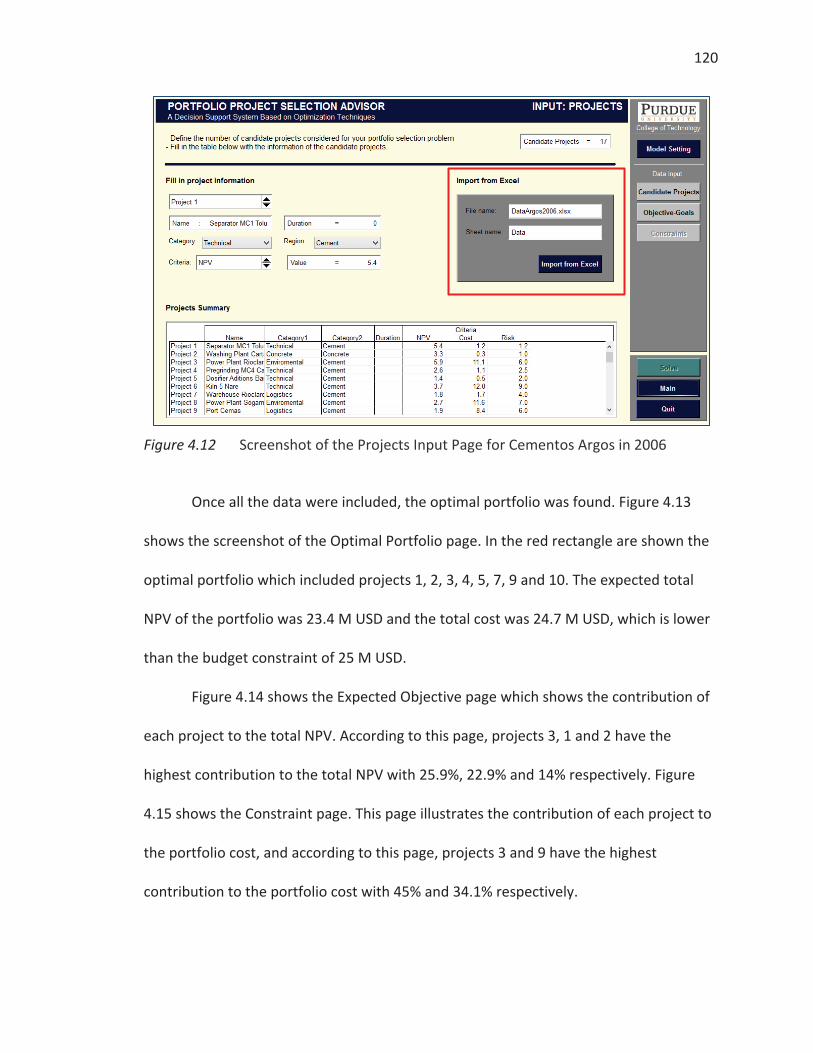
120
Figure 4.12 Screenshot of the Projects Input Page for Cementos Argos in 2006
Once all the data were included, the optimal portfolio was found. Figure 4.13
shows the screenshot of the Optimal Portfolio page. In the red rectangle are shown the
optimal portfolio which included projects 1, 2, 3, 4, 5, 7, 9 and 10. The expected total
NPV of the portfolio was 23.4 M USD and the total cost was 24.7 M USD, which is lower
than the budget constraint of 25 M USD.
Figure 4.14 shows the Expected Objective page which shows the contribution of
each project to the total NPV. According to this page, projects 3, 1 and 2 have the
highest contribution to the total NPV with 25.9%, 22.9% and 14% respectively. Figure
4.15 shows the Constraint page. This page illustrates the contribution of each project to
the portfolio cost, and according to this page, projects 3 and 9 have the highest
contribution to the portfolio cost with 45% and 34.1% respectively.
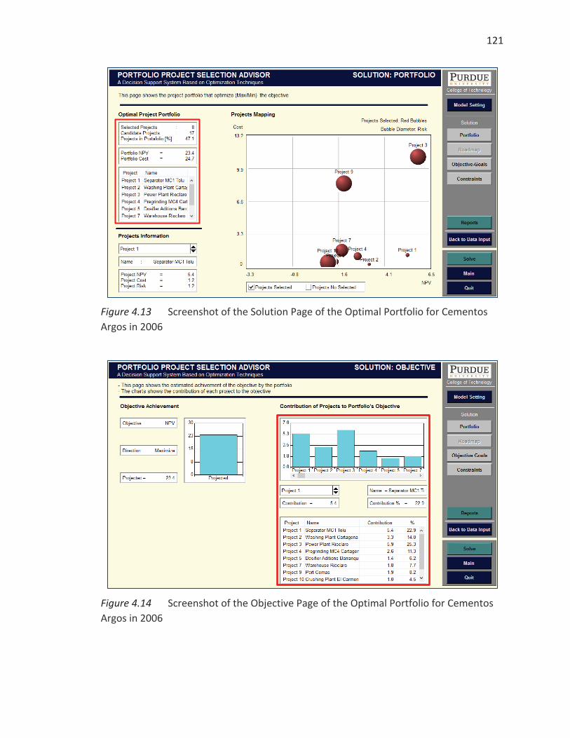
121
Figure 4.13 Screenshot of the Solution Page of the Optimal Portfolio for Cementos Argos in 2006
Figure 4.14 Screenshot of the Objective Page of the Optimal Portfolio for Cementos Argos in 2006
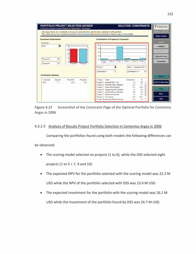
122
Figure 4.15 Screenshot of the Constraint Page of the Optimal Portfolio for Cementos Argos in 2006
4.3.2.3 Analysis of Results Project Portfolio Selection in Cementos Argos in 2006
Comparing the portfolios found using both models the following differences can
be observed:
The scoring model selected six projects (1 to 6), while the DSS selected eight
projects (1 to 5 + 7, 9 and 10).
The expected NPV for the portfolio selected with the scoring model was 22.3 M
USD while the NPV of the portfolio selected with DSS was 23.4 M USD
The expected investment for the portfolio with the scoring model was 26.2 M
USD while the investment of the portfolio found by DSS was 24.7 M USD.
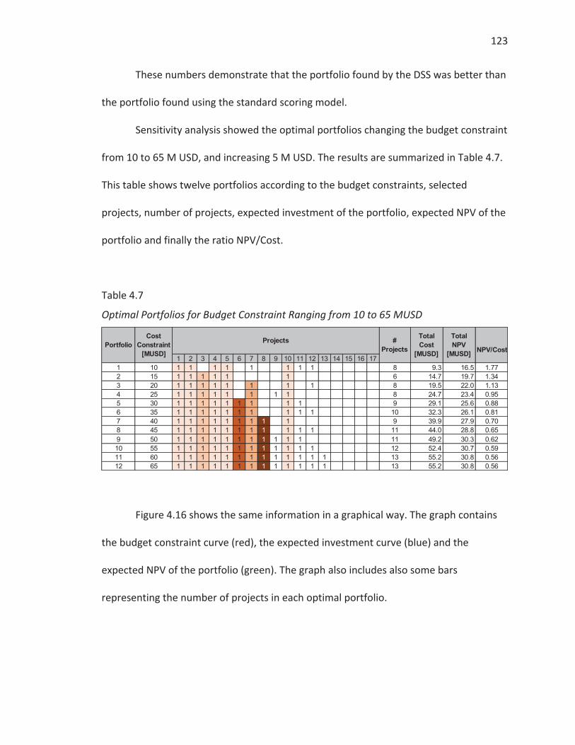
123
These numbers demonstrate that the portfolio found by the DSS was better than
the portfolio found using the standard scoring model.
Sensitivity analysis showed the optimal portfolios changing the budget constraint
from 10 to 65 M USD, and increasing 5 M USD. The results are summarized in Table 4.7.
This table shows twelve portfolios according to the budget constraints, selected
projects, number of projects, expected investment of the portfolio, expected NPV of the
portfolio and finally the ratio NPV/Cost.
Table 4.7
Optimal Portfolios for Budget Constraint Ranging from 10 to 65 MUSD
Figure 4.16 shows the same information in a graphical way. The graph contains
the budget constraint curve (red), the expected investment curve (blue) and the
expected NPV of the portfolio (green). The graph also includes also some bars
representing the number of projects in each optimal portfolio.
NPV/Cost1 2 3 4 5 6 7 8 9 10 11 12 13 14 15 16 17
1 10 1 1 1 1 1 1 1 1 8 9.3 16.5 1.772 15 1 1 1 1 1 1 6 14.7 19.7 1.343 20 1 1 1 1 1 1 1 1 8 19.5 22.0 1.134 25 1 1 1 1 1 1 1 1 8 24.7 23.4 0.955 30 1 1 1 1 1 1 1 1 1 9 29.1 25.6 0.886 35 1 1 1 1 1 1 1 1 1 1 10 32.3 26.1 0.817 40 1 1 1 1 1 1 1 1 1 9 39.9 27.9 0.708 45 1 1 1 1 1 1 1 1 1 1 1 11 44.0 28.8 0.659 50 1 1 1 1 1 1 1 1 1 1 1 11 49.2 30.3 0.6210 55 1 1 1 1 1 1 1 1 1 1 1 1 12 52.4 30.7 0.5911 60 1 1 1 1 1 1 1 1 1 1 1 1 1 13 55.2 30.8 0.5612 65 1 1 1 1 1 1 1 1 1 1 1 1 1 13 55.2 30.8 0.56
Portfolio Projects Total Cost
[MUSD]
Total NPV
[MUSD]
# Projects
Cost Constraint
[MUSD]
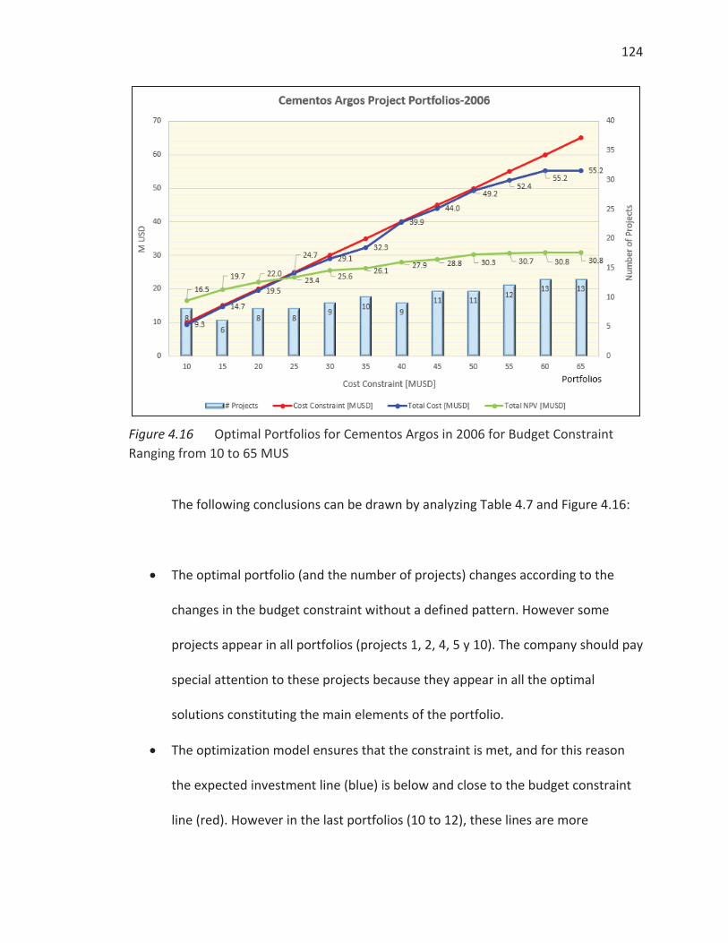
124
Figure 4.16 Optimal Portfolios for Cementos Argos in 2006 for Budget Constraint Ranging from 10 to 65 MUS
The following conclusions can be drawn by analyzing Table 4.7 and Figure 4.16:
The optimal portfolio (and the number of projects) changes according to the
changes in the budget constraint without a defined pattern. However some
projects appear in all portfolios (projects 1, 2, 4, 5 y 10). The company should pay
special attention to these projects because they appear in all the optimal
solutions constituting the main elements of the portfolio.
The optimization model ensures that the constraint is met, and for this reason
the expected investment line (blue) is below and close to the budget constraint
line (red). However in the last portfolios (10 to 12), these lines are more

125
separated because the DSS did not find better projects to include in the
portfolio.
The NPV line (green) at the beginning is above the expected investment line
(blue), however, in the following portfolios, the lines intercepts and then the
NPV line continues below the expected investment line. This can be explained in
the following way: the best projects are chosen in the first portfolios (with the
lower budget constraint), then the DSS chose goods projects and finally the DSS
selected the projects that add some value in the last portfolios (with higher
budget constraint). The profitability of the portfolio decreases as the slope of the
NPV curve approximates zero in the last portfolios. This seems to be a pattern in
this kind of problems.
The company could define the investment budget as a function of the candidate
projects and the expected profitability of the portfolio. This could change from
year to year, according to the potential of the candidate projects to add value to
the organization.
4.3.3 Project Portfolio Selection in Cementos Argos in 2014
In 2014, the company is considering 102 candidate projects for execution for
2015. The list of these projects includes cost, NPV and Payback. Table 4.8 shows the
candidate projects. The name of the projects is changed for confidential reasons and
Payback is considered here a risk measure.

126
Table 4.8
Candidate Projects Considered by Cementos Argos in 2014
(continued)
Project Name Category1 Category2 DurationNPV
[K USD]Cost
[K USD] Risk PayBackProject 1 Proyecto 1 Caribbean Concrete 60.0 400 3.42 3.42Project 2 Proyecto 3 Caribbean Concrete 25.2 140 5.75 5.75Project 3 Proyecto 4 Caribbean Concrete 9.0 45 4.50 4.50Project 4 Proyecto 5 Caribbean Concrete 20.0 80 2.42 2.42Project 5 Proyecto 6 Caribbean Concrete 13.5 30 6.67 6.67Project 6 Proyecto 7 Caribbean Concrete 192.0 400 6.83 6.83Project 7 Proyecto 8 Caribbean Concrete 4.8 80 4.25 4.25Project 8 Proyecto 9 Caribbean Concrete 893.0 1,900 3.08 3.08Project 9 Proyecto 10 Caribbean Cement 182.7 1,075 6.33 6.33Project 10 Proyecto 11 USA Cement 804.7 2,515 4.75 4.75Project 11 Proyecto 12 USA Cement 200.0 400 5.83 5.83Project 12 Proyecto 13 USA Cement 28.9 85 3.17 3.17Project 13 Proyecto 14 USA Cement 235.0 500 1.00 1.00Project 14 Proyecto 15 USA Cement 9.0 450 2.67 2.67Project 15 Proyecto 16 USA Cement 9.9 90 5.75 5.75Project 16 Proyecto 17 USA Cement 180.0 600 2.58 2.58Project 17 Proyecto 18 USA Cement 157.5 450 5.75 5.75Project 18 Proyecto 19 USA Cement 137.5 275 5.25 5.25Project 19 Proyecto 20 USA Cement 50.0 200 2.83 2.83Project 20 Proyecto 21 USA Cement 9.0 100 6.00 6.00Project 21 Proyecto 22 USA Cement 27.0 100 0.83 0.83Project 22 Proyecto 23 USA Cement 30.0 100 1.58 1.58Project 23 Proyecto 24 USA Cement 576.0 1,200 5.25 5.25Project 24 Proyecto 25 USA Cement 277.5 5,550 4.08 4.08Project 25 Proyecto 26 USA Cement 837.0 3,100 6.83 6.83Project 26 Proyecto 27 USA Concrete 2,760.0 6,000 4.17 4.17Project 27 Proyecto 28 USA Concrete 21.6 120 3.67 3.67Project 28 Proyecto 29 USA Concrete 26.5 115 4.33 4.33Project 29 Proyecto 30 USA Concrete 75.0 300 3.00 3.00Project 30 Proyecto 31 USA Concrete 470.0 1,000 0.75 0.75Project 31 Proyecto 32 USA Concrete 108.5 350 5.75 5.75Project 32 Proyecto 33 Colombia Cement 44.8 149 6.42 6.42Project 33 Proyecto 34 Colombia Cement 1,380.0 3,000 1.33 1.33Project 34 Proyecto 35 Colombia Cement 26.9 149 5.92 5.92Project 35 Proyecto 36 Colombia Cement 45.8 100 4.50 4.50Project 36 Proyecto 37 Colombia Cement 477.6 995 4.25 4.25Project 37 Proyecto 38 Colombia Cement 78.4 174 2.58 2.58Project 38 Proyecto 39 Colombia Cement 174.1 498 1.92 1.92Project 39 Proyecto 40 Colombia Cement 43.0 239 3.75 3.75Project 40 Proyecto 41 Colombia Cement 84.6 498 6.17 6.17Project 41 Proyecto 42 Colombia Cement 59.7 299 1.58 1.58Project 42 Proyecto 43 Colombia Cement 53.3 157 3.00 3.00Project 43 Proyecto 44 Colombia Cement 44.8 100 2.17 2.17Project 44 Proyecto 45 Colombia Cement 7.5 50 6.75 6.75Project 45 Proyecto 46 Colombia Cement 140.3 299 4.50 4.50Project 46 Proyecto 47 Colombia Cement 16.9 100 6.58 6.58Project 47 Proyecto 48 Colombia Cement 17.9 100 6.67 6.67Project 48 Proyecto 49 Colombia Cement 1,474.0 3,008 4.33 4.33Project 49 Proyecto 50 Colombia Cement 437.3 2,186 4.25 4.25Project 50 Proyecto 52 Colombia Cement 207.9 2,599 1.17 1.17Project 51 Proyecto 53 Colombia Cement 1,507.9 3,077 2.17 2.17
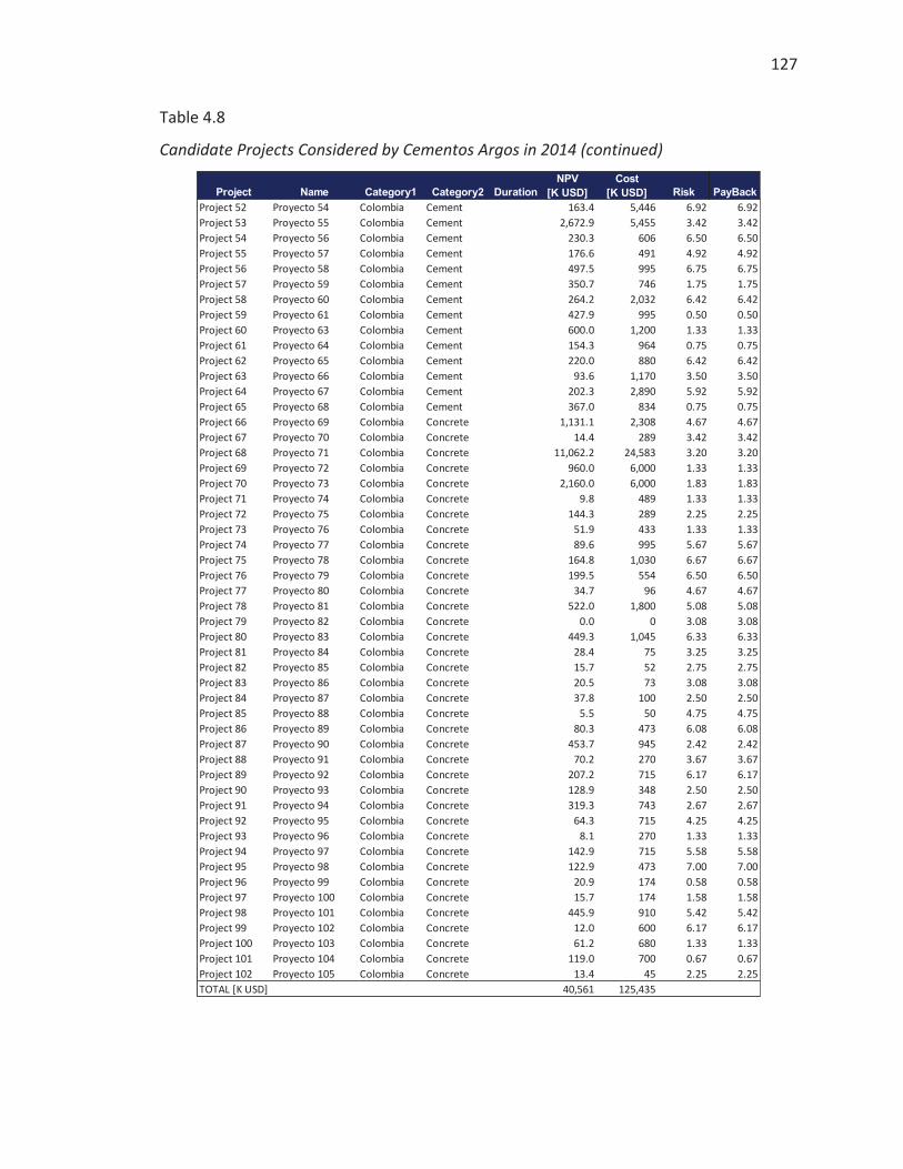
127
Table 4.8
Candidate Projects Considered by Cementos Argos in 2014 (continued)
Project Name Category1 Category2 DurationNPV
[K USD]Cost
[K USD] Risk PayBackProject 52 Proyecto 54 Colombia Cement 163.4 5,446 6.92 6.92Project 53 Proyecto 55 Colombia Cement 2,672.9 5,455 3.42 3.42Project 54 Proyecto 56 Colombia Cement 230.3 606 6.50 6.50Project 55 Proyecto 57 Colombia Cement 176.6 491 4.92 4.92Project 56 Proyecto 58 Colombia Cement 497.5 995 6.75 6.75Project 57 Proyecto 59 Colombia Cement 350.7 746 1.75 1.75Project 58 Proyecto 60 Colombia Cement 264.2 2,032 6.42 6.42Project 59 Proyecto 61 Colombia Cement 427.9 995 0.50 0.50Project 60 Proyecto 63 Colombia Cement 600.0 1,200 1.33 1.33Project 61 Proyecto 64 Colombia Cement 154.3 964 0.75 0.75Project 62 Proyecto 65 Colombia Cement 220.0 880 6.42 6.42Project 63 Proyecto 66 Colombia Cement 93.6 1,170 3.50 3.50Project 64 Proyecto 67 Colombia Cement 202.3 2,890 5.92 5.92Project 65 Proyecto 68 Colombia Cement 367.0 834 0.75 0.75Project 66 Proyecto 69 Colombia Concrete 1,131.1 2,308 4.67 4.67Project 67 Proyecto 70 Colombia Concrete 14.4 289 3.42 3.42Project 68 Proyecto 71 Colombia Concrete 11,062.2 24,583 3.20 3.20Project 69 Proyecto 72 Colombia Concrete 960.0 6,000 1.33 1.33Project 70 Proyecto 73 Colombia Concrete 2,160.0 6,000 1.83 1.83Project 71 Proyecto 74 Colombia Concrete 9.8 489 1.33 1.33Project 72 Proyecto 75 Colombia Concrete 144.3 289 2.25 2.25Project 73 Proyecto 76 Colombia Concrete 51.9 433 1.33 1.33Project 74 Proyecto 77 Colombia Concrete 89.6 995 5.67 5.67Project 75 Proyecto 78 Colombia Concrete 164.8 1,030 6.67 6.67Project 76 Proyecto 79 Colombia Concrete 199.5 554 6.50 6.50Project 77 Proyecto 80 Colombia Concrete 34.7 96 4.67 4.67Project 78 Proyecto 81 Colombia Concrete 522.0 1,800 5.08 5.08Project 79 Proyecto 82 Colombia Concrete 0.0 0 3.08 3.08Project 80 Proyecto 83 Colombia Concrete 449.3 1,045 6.33 6.33Project 81 Proyecto 84 Colombia Concrete 28.4 75 3.25 3.25Project 82 Proyecto 85 Colombia Concrete 15.7 52 2.75 2.75Project 83 Proyecto 86 Colombia Concrete 20.5 73 3.08 3.08Project 84 Proyecto 87 Colombia Concrete 37.8 100 2.50 2.50Project 85 Proyecto 88 Colombia Concrete 5.5 50 4.75 4.75Project 86 Proyecto 89 Colombia Concrete 80.3 473 6.08 6.08Project 87 Proyecto 90 Colombia Concrete 453.7 945 2.42 2.42Project 88 Proyecto 91 Colombia Concrete 70.2 270 3.67 3.67Project 89 Proyecto 92 Colombia Concrete 207.2 715 6.17 6.17Project 90 Proyecto 93 Colombia Concrete 128.9 348 2.50 2.50Project 91 Proyecto 94 Colombia Concrete 319.3 743 2.67 2.67Project 92 Proyecto 95 Colombia Concrete 64.3 715 4.25 4.25Project 93 Proyecto 96 Colombia Concrete 8.1 270 1.33 1.33Project 94 Proyecto 97 Colombia Concrete 142.9 715 5.58 5.58Project 95 Proyecto 98 Colombia Concrete 122.9 473 7.00 7.00Project 96 Proyecto 99 Colombia Concrete 20.9 174 0.58 0.58Project 97 Proyecto 100 Colombia Concrete 15.7 174 1.58 1.58Project 98 Proyecto 101 Colombia Concrete 445.9 910 5.42 5.42Project 99 Proyecto 102 Colombia Concrete 12.0 600 6.17 6.17Project 100 Proyecto 103 Colombia Concrete 61.2 680 1.33 1.33Project 101 Proyecto 104 Colombia Concrete 119.0 700 0.67 0.67Project 102 Proyecto 105 Colombia Concrete 13.4 45 2.25 2.25TOTAL [K USD] 40,561 125,435
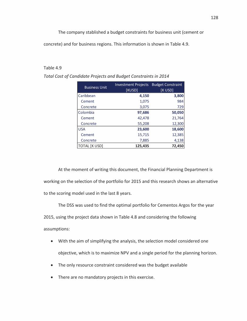
128
The company stablished a budget constraints for business unit (cement or
concrete) and for business regions. This information is shown in Table 4.9.
Table 4.9
Total Cost of Candidate Projects and Budget Constraints in 2014
At the moment of writing this document, the Financial Planning Department is
working on the selection of the portfolio for 2015 and this research shows an alternative
to the scoring model used in the last 8 years.
The DSS was used to find the optimal portfolio for Cementos Argos for the year
2015, using the project data shown in Table 4.8 and considering the following
assumptions:
With the aim of simplifying the analysis, the selection model considered one
objective, which is to maximize NPV and a single period for the planning horizon.
The only resource constraint considered was the budget available
There are no mandatory projects in this exercise.
Business UnitInvestment Projects
[KUSD]Budget Constraint
[K USD]Caribbean 4,150 3,800
Cement 1,075 984Concrete 3,075 729
Colombia 97,686 50,050Cement 42,478 21,764Concrete 55,208 12,300
USA 23,600 18,600Cement 15,715 12,385Concrete 7,885 4,138
TOTAL [K USD] 125,435 72,450
129
There is no relationship of dependency among candidate projects.
Two approaches are proposed to find the optimal portfolio according to the
resource constraints defined by the company and showed in Table 4.9 as follows:
1. Portfolio selection for the entire company, meaning, globally optimizing the
portfolio according to the total budget constraint of 72,450 K USD. This
means, finding the optimal portfolio for the company with all candidate
projects from all regions competing for the resources.
2. Portfolio selection per region, meaning, locally optimizing the portfolios
according to the budget constraints defined per region which are 3,800 K
USD for the Caribbean, 18,600 K USD for USA and 50,050 K USD for
Colombia. Then, this means finding the optimal portfolio per region with the
projects and the budget associated with each region.
Other alternative approaches can be studied, for example, optimizing the
portfolio by considering the budget constraint per business unit (cement or concrete
business), however, for the Financial Planning Department is more interested in the
analysis per regions. The purpose of studying these approaches is to compare and
analyze the solutions found in each case and make a recommendation.

130
4.3.3.1 Project Portfolio Selection in Cementos Argos in 2014-Global Optimization
In this selection process, 102 candidate projects were considered, all in
competition, and the budget constraint is 72,450 KUSD. The following paragraphs
illustrate some screenshots with the use of the DSS and the results.
Initially the test is configured on the DSS for one objective and a single period of
time; then data of the candidate projects, objective and budget constraint are
introduced. Figure 4.17 shows the screenshot of the projects input page.
Figure 4.17 Screenshot of the Projects Input Page for Cementos Argos in 2014.
Once all the data are included, the optimal portfolio is found. Figure 4.18 shows
the screenshot of the Optimal Portfolio page. Forty projects were selected, the expected
NPV of the portfolio was 32,771.6 K USD and the total cost was 72,439 K USD, which is
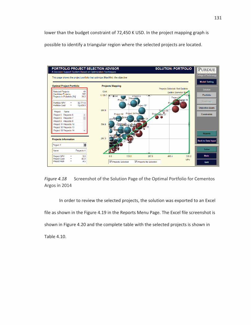
131
lower than the budget constraint of 72,450 K USD. In the project mapping graph is
possible to identify a triangular region where the selected projects are located.
Figure 4.18 Screenshot of the Solution Page of the Optimal Portfolio for Cementos Argos in 2014
In order to review the selected projects, the solution was exported to an Excel
file as shown in the Figure 4.19 in the Reports Menu Page. The Excel file screenshot is
shown in Figure 4.20 and the complete table with the selected projects is shown in
Table 4.10.
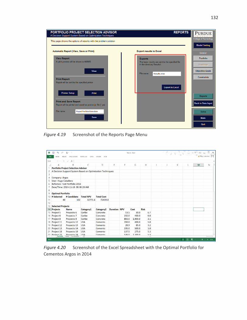
132
Figure 4.19 Screenshot of the Reports Page Menu
Figure 4.20 Screenshot of the Excel Spreadsheet with the Optimal Portfolio for Cementos Argos in 2014

133
Table 4.10
Optimal Portfolio in Cementos Argos According to Global Optimization in 2014
Projects Name Category1 Category2 NPV Cost RiskProject 5 Proyecto 6 Caribe Concreto 13.5 30.0 6.7Project 6 Proyecto 7 Caribe Concreto 192.0 400.0 6.8Project 8 Proyecto 9 Caribe Concreto 893.0 1,900.0 3.1Project 11 Proyecto 12 USA Cemento 200.0 400.0 5.8Project 12 Proyecto 13 USA Cemento 28.9 85.0 3.2Project 13 Proyecto 14 USA Cemento 235.0 500.0 1.0Project 18 Proyecto 19 USA Cemento 137.5 275.0 5.3Project 23 Proyecto 24 USA Cemento 576.0 1,200.0 5.3Project 26 Proyecto 27 USA Concreto 2,760.0 6,000.0 4.2Project 30 Proyecto 31 USA Concreto 470.0 1,000.0 0.8Project 33 Proyecto 34 Colombia Cemento 1,380.0 3,000.0 1.3Project 35 Proyecto 36 Colombia Cemento 45.8 99.5 4.5Project 36 Proyecto 37 Colombia Cemento 477.6 995.0 4.3Project 37 Proyecto 38 Colombia Cemento 78.4 174.1 2.6Project 38 Proyecto 39 Colombia Cemento 174.1 497.5 1.9Project 42 Proyecto 43 Colombia Cemento 53.3 156.7 3.0Project 43 Proyecto 44 Colombia Cemento 44.8 99.5 2.2Project 45 Proyecto 46 Colombia Cemento 140.3 298.5 4.5Project 48 Proyecto 49 Colombia Cemento 1,474.0 3,008.2 4.3Project 51 Proyecto 53 Colombia Cemento 1,507.9 3,077.4 2.2Project 53 Proyecto 55 Colombia Cemento 2,672.9 5,454.9 3.4Project 54 Proyecto 56 Colombia Cemento 230.3 606.0 6.5Project 55 Proyecto 57 Colombia Cemento 176.6 490.5 4.9Project 56 Proyecto 58 Colombia Cemento 497.5 995.0 6.8Project 57 Proyecto 59 Colombia Cemento 350.7 746.3 1.8Project 59 Proyecto 61 Colombia Cemento 427.9 995.0 0.5Project 60 Proyecto 63 Colombia Cemento 600.0 1,200.0 1.3Project 65 Proyecto 68 Colombia Cemento 367.0 834.0 0.8Project 66 Proyecto 69 Colombia Concreto 1,131.1 2,308.5 4.7Project 68 Proyecto 71 Colombia Concreto 11,062.2 24,582.7 3.2Project 70 Proyecto 73 Colombia Concreto 2,160.0 6,000.0 1.8Project 72 Proyecto 75 Colombia Concreto 144.3 288.6 2.3Project 76 Proyecto 79 Colombia Concreto 199.5 554.3 6.5Project 77 Proyecto 80 Colombia Concreto 34.7 96.4 4.7Project 80 Proyecto 83 Colombia Concreto 449.3 1,044.8 6.3Project 84 Proyecto 87 Colombia Concreto 37.8 99.5 2.5Project 87 Proyecto 90 Colombia Concreto 453.7 945.3 2.4Project 90 Proyecto 93 Colombia Concreto 128.9 348.3 2.5Project 91 Proyecto 94 Colombia Concreto 319.3 742.5 2.7Project 98 Proyecto 101 Colombia Concreto 445.9 910.0 5.4TOTAL 32,771.6 72,439.0
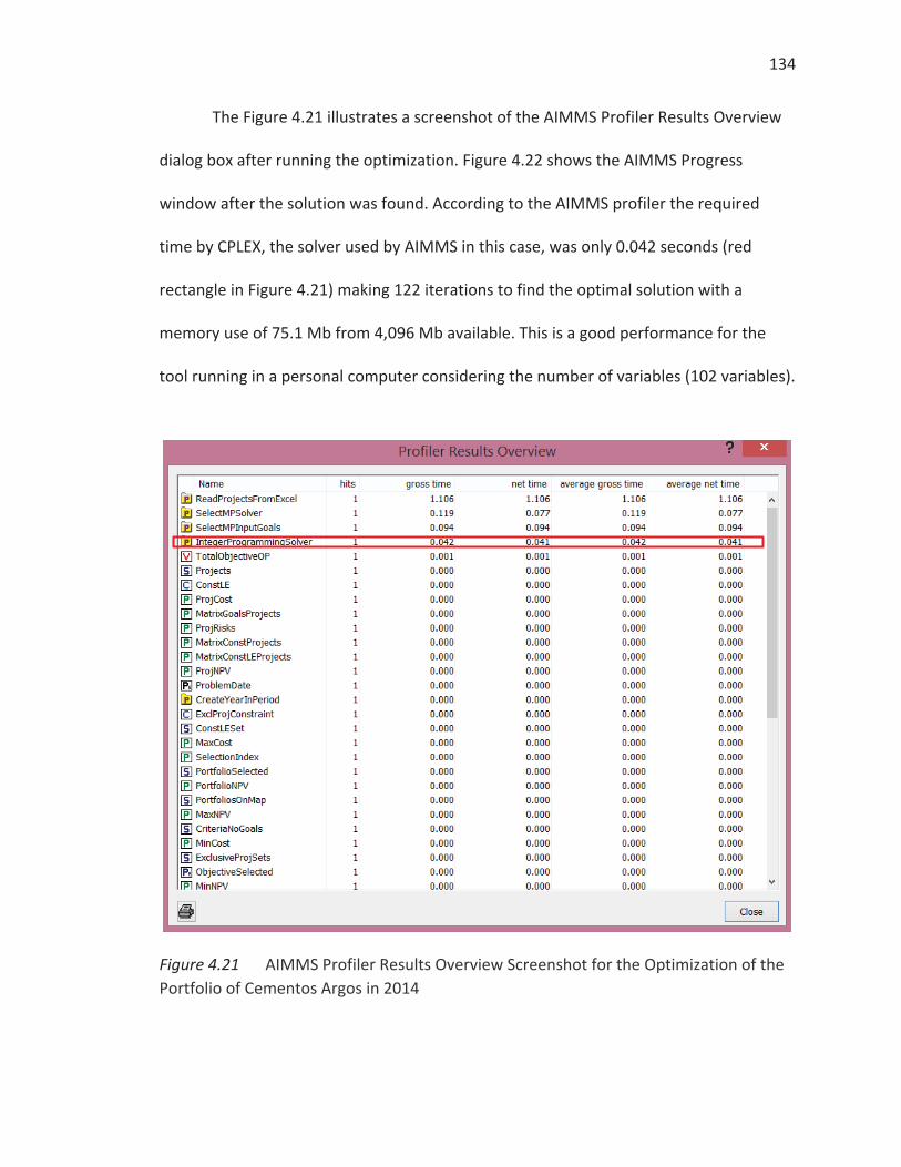
134
The Figure 4.21 illustrates a screenshot of the AIMMS Profiler Results Overview
dialog box after running the optimization. Figure 4.22 shows the AIMMS Progress
window after the solution was found. According to the AIMMS profiler the required
time by CPLEX, the solver used by AIMMS in this case, was only 0.042 seconds (red
rectangle in Figure 4.21) making 122 iterations to find the optimal solution with a
memory use of 75.1 Mb from 4,096 Mb available. This is a good performance for the
tool running in a personal computer considering the number of variables (102 variables).
Figure 4.21 AIMMS Profiler Results Overview Screenshot for the Optimization of the Portfolio of Cementos Argos in 2014
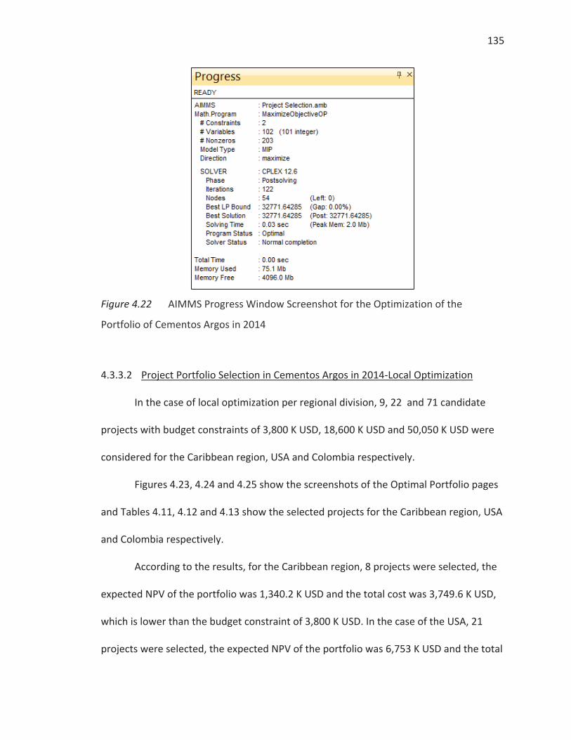
135
Figure 4.22 AIMMS Progress Window Screenshot for the Optimization of the
Portfolio of Cementos Argos in 2014
4.3.3.2 Project Portfolio Selection in Cementos Argos in 2014-Local Optimization
In the case of local optimization per regional division, 9, 22 and 71 candidate
projects with budget constraints of 3,800 K USD, 18,600 K USD and 50,050 K USD were
considered for the Caribbean region, USA and Colombia respectively.
Figures 4.23, 4.24 and 4.25 show the screenshots of the Optimal Portfolio pages
and Tables 4.11, 4.12 and 4.13 show the selected projects for the Caribbean region, USA
and Colombia respectively.
According to the results, for the Caribbean region, 8 projects were selected, the
expected NPV of the portfolio was 1,340.2 K USD and the total cost was 3,749.6 K USD,
which is lower than the budget constraint of 3,800 K USD. In the case of the USA, 21
projects were selected, the expected NPV of the portfolio was 6,753 K USD and the total
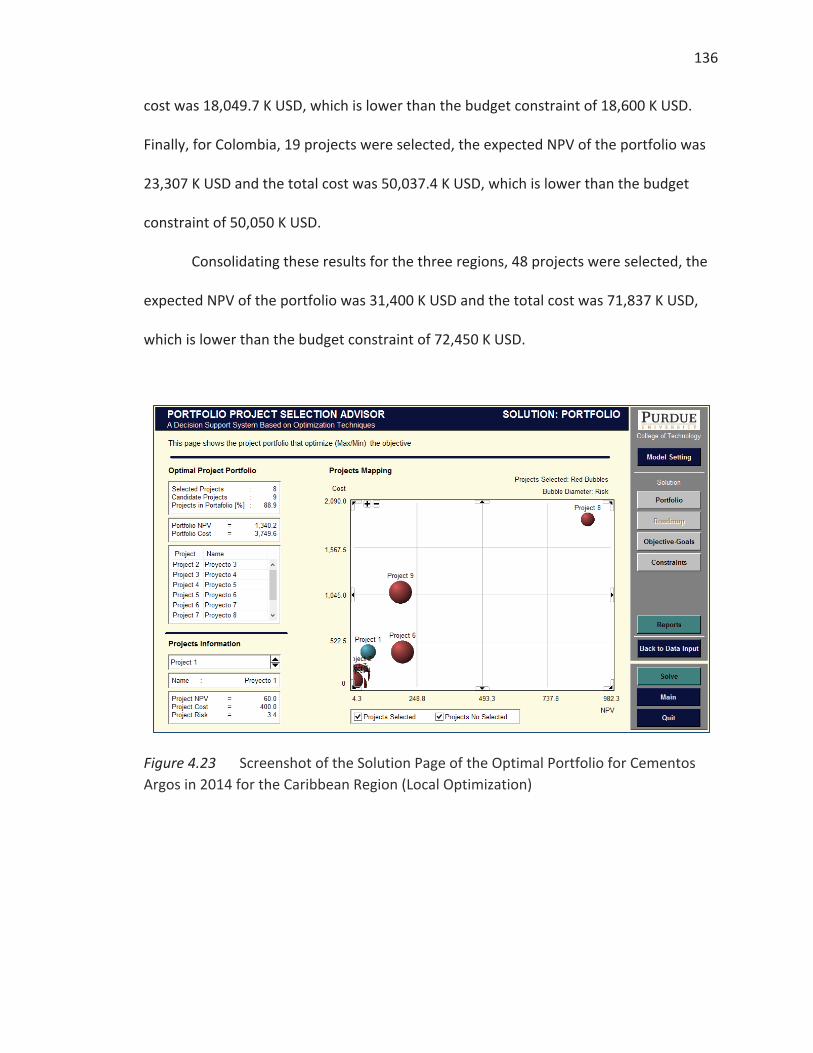
136
cost was 18,049.7 K USD, which is lower than the budget constraint of 18,600 K USD.
Finally, for Colombia, 19 projects were selected, the expected NPV of the portfolio was
23,307 K USD and the total cost was 50,037.4 K USD, which is lower than the budget
constraint of 50,050 K USD.
Consolidating these results for the three regions, 48 projects were selected, the
expected NPV of the portfolio was 31,400 K USD and the total cost was 71,837 K USD,
which is lower than the budget constraint of 72,450 K USD.
Figure 4.23 Screenshot of the Solution Page of the Optimal Portfolio for Cementos Argos in 2014 for the Caribbean Region (Local Optimization)
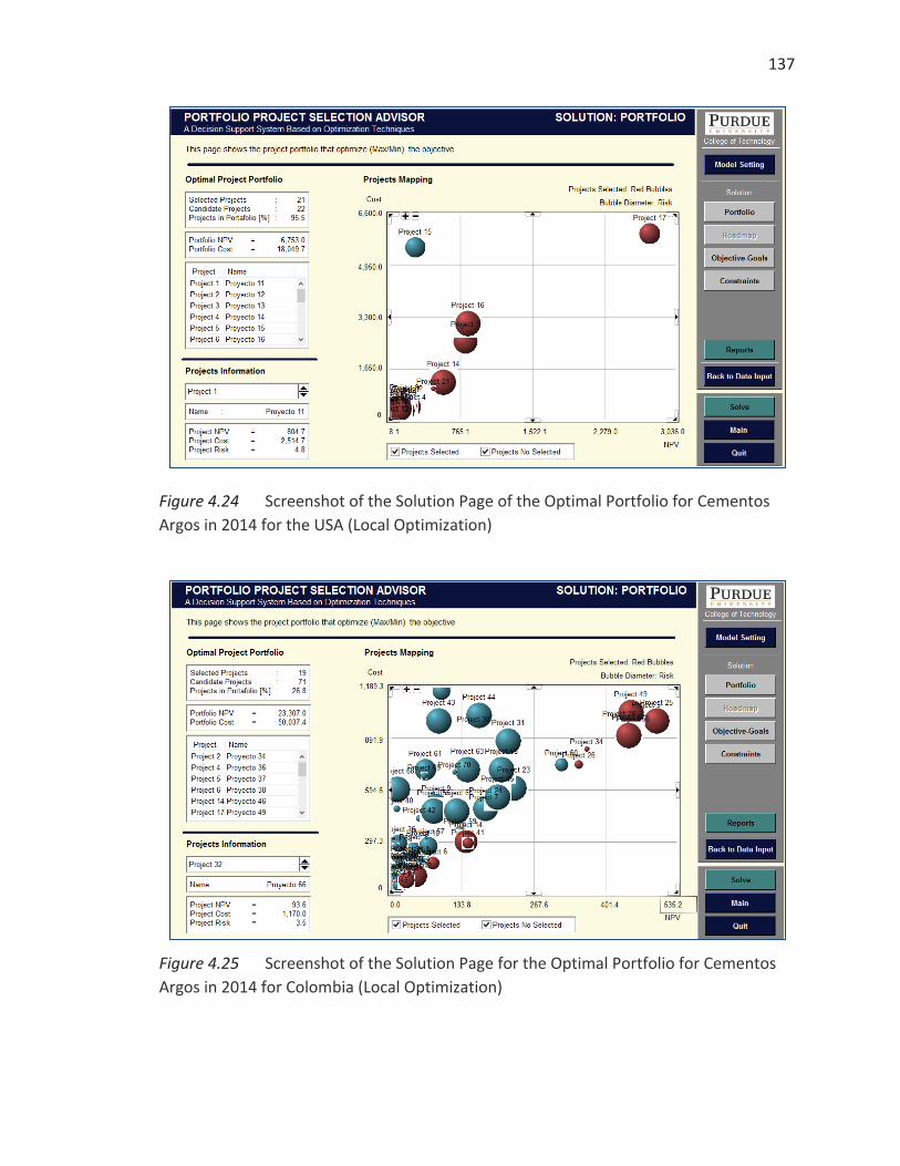
137
Figure 4.24 Screenshot of the Solution Page of the Optimal Portfolio for Cementos Argos in 2014 for the USA (Local Optimization)
Figure 4.25 Screenshot of the Solution Page for the Optimal Portfolio for Cementos Argos in 2014 for Colombia (Local Optimization)

138
Table 4.11
Optimal Portfolio in Cementos Argos According to Local Optimization for the Caribbean Regional Division in 2014
Table 4.12
Optimal Portfolio in Argos According to Local Optimization for the USA Regional Division in 2014
Projects Name Category1 Category2 NPV [K USD] Cost [K USD] RiskProject 2 Proyecto 3 Caribbean Concrete 25.2 140.0 5.8Project 3 Proyecto 4 Caribbean Concrete 9.0 45.0 4.5Project 4 Proyecto 5 Caribbean Concrete 20.0 80.0 2.4Project 5 Proyecto 6 Caribbean Concrete 13.5 30.0 6.7Project 6 Proyecto 7 Caribbean Concrete 192.0 400.0 6.8Project 7 Proyecto 8 Caribbean Concrete 4.8 80.0 4.3Project 8 Proyecto 9 Caribbean Concrete 893.0 1,900.0 3.1Project 9 Proyecto 10 Caribbean Cement 182.7 1,074.6 6.3TOTAL 1,340.2 3,749.6
Projects Name Category1 Category2 NPV [K USD] Cost [K USD] RiskProject 1 Proyecto 11 USA Cement 804.7 2514.7 4.8Project 2 Proyecto 12 USA Cement 200.0 400.0 5.8Project 3 Proyecto 13 USA Cement 28.9 85.0 3.2Project 4 Proyecto 14 USA Cement 235.0 500.0 1.0Project 5 Proyecto 15 USA Cement 9.0 450.0 2.7Project 6 Proyecto 16 USA Cement 9.9 90.0 5.8Project 7 Proyecto 17 USA Cement 180.0 600.0 2.6Project 8 Proyecto 18 USA Cement 157.5 450.0 5.8Project 9 Proyecto 19 USA Cement 137.5 275.0 5.3Project 10 Proyecto 20 USA Cement 50.0 200.0 2.8Project 11 Proyecto 21 USA Cement 9.0 100.0 6.0Project 12 Proyecto 22 USA Cement 27.0 100.0 0.8Project 13 Proyecto 23 USA Cement 30.0 100.0 1.6Project 14 Proyecto 24 USA Cement 576.0 1200.0 5.3Project 16 Proyecto 26 USA Cement 837.0 3100.0 6.8Project 17 Proyecto 27 USA Concrete 2760.0 6000.0 4.2Project 18 Proyecto 28 USA Concrete 21.6 120.0 3.7Project 19 Proyecto 29 USA Concrete 26.5 115.0 4.3Project 20 Proyecto 30 USA Concrete 75.0 300.0 3.0Project 21 Proyecto 31 USA Concrete 470.0 1000.0 0.8Project 22 Proyecto 32 USA Concrete 108.5 350.0 5.8TOTAL 6753.0 18049.7
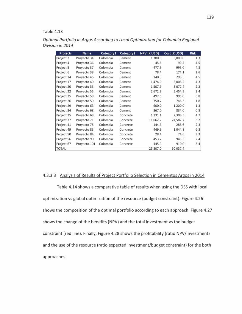
139
Table 4.13
Optimal Portfolio in Argos According to Local Optimization for Colombia Regional Division in 2014
4.3.3.3 Analysis of Results of Project Portfolio Selection in Cementos Argos in 2014
Table 4.14 shows a comparative table of results when using the DSS with local
optimization vs global optimization of the resource (budget constraint). Figure 4.26
shows the composition of the optimal portfolio according to each approach. Figure 4.27
shows the change of the benefits (NPV) and the total investment vs the budget
constraint (red line). Finally, Figure 4.28 shows the profitability (ratio NPV/Investment)
and the use of the resource (ratio expected investment/budget constraint) for the both
approaches.
Projects Name Category1 Category2 NPV [K USD] Cost [K USD] RiskProject 2 Proyecto 34 Colombia Cement 1,380.0 3,000.0 1.3Project 4 Proyecto 36 Colombia Cement 45.8 99.5 4.5Project 5 Proyecto 37 Colombia Cement 477.6 995.0 4.3Project 6 Proyecto 38 Colombia Cement 78.4 174.1 2.6Project 14 Proyecto 46 Colombia Cement 140.3 298.5 4.5Project 17 Proyecto 49 Colombia Cement 1,474.0 3,008.2 4.3Project 20 Proyecto 53 Colombia Cement 1,507.9 3,077.4 2.2Project 22 Proyecto 55 Colombia Cement 2,672.9 5,454.9 3.4Project 25 Proyecto 58 Colombia Cement 497.5 995.0 6.8Project 26 Proyecto 59 Colombia Cement 350.7 746.3 1.8Project 29 Proyecto 63 Colombia Cement 600.0 1,200.0 1.3Project 34 Proyecto 68 Colombia Cement 367.0 834.0 0.8Project 35 Proyecto 69 Colombia Concrete 1,131.1 2,308.5 4.7Project 37 Proyecto 71 Colombia Concrete 11,062.2 24,582.7 3.2Project 41 Proyecto 75 Colombia Concrete 144.3 288.6 2.3Project 49 Proyecto 83 Colombia Concrete 449.3 1,044.8 6.3Project 50 Proyecto 84 Colombia Concrete 28.4 74.6 3.3Project 56 Proyecto 90 Colombia Concrete 453.7 945.3 2.4Project 67 Proyecto 101 Colombia Concrete 445.9 910.0 5.4TOTAL 23,307.0 50,037.4
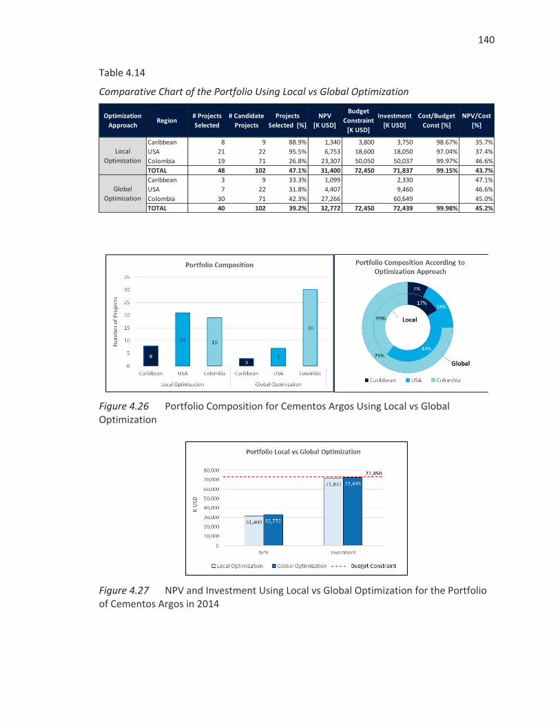
140
Table 4.14
Comparative Chart of the Portfolio Using Local vs Global Optimization
Figure 4.26 Portfolio Composition for Cementos Argos Using Local vs Global Optimization
Figure 4.27 NPV and Investment Using Local vs Global Optimization for the Portfolio of Cementos Argos in 2014
Optimization Approach
Region# Projects Selected
# Candidate Projects
Projects Selected [%]
NPV [K USD]
Budget Constraint
[K USD]
Investment [K USD]
Cost/Budget Const [%]
NPV/Cost [%]
Caribbean 8 9 88.9% 1,340 3,800 3,750 98.67% 35.7%USA 21 22 95.5% 6,753 18,600 18,050 97.04% 37.4%Colombia 19 71 26.8% 23,307 50,050 50,037 99.97% 46.6%TOTAL 48 102 47.1% 31,400 72,450 71,837 99.15% 43.7%Caribbean 3 9 33.3% 1,099 2,330 47.1%USA 7 22 31.8% 4,407 9,460 46.6%Colombia 30 71 42.3% 27,266 60,649 45.0%TOTAL 40 102 39.2% 32,772 72,450 72,439 99.98% 45.2%
Local Optimization
Global Optimization
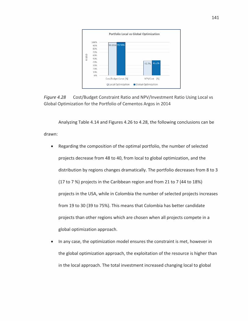
141
Figure 4.28 Cost/Budget Constraint Ratio and NPV/Investment Ratio Using Local vs Global Optimization for the Portfolio of Cementos Argos in 2014
Analyzing Table 4.14 and Figures 4.26 to 4.28, the following conclusions can be
drawn:
Regarding the composition of the optimal portfolio, the number of selected
projects decrease from 48 to 40, from local to global optimization, and the
distribution by regions changes dramatically. The portfolio decreases from 8 to 3
(17 to 7 %) projects in the Caribbean region and from 21 to 7 (44 to 18%)
projects in the USA, while in Colombia the number of selected projects increases
from 19 to 30 (39 to 75%). This means that Colombia has better candidate
projects than other regions which are chosen when all projects compete in a
global optimization approach.
In any case, the optimization model ensures the constraint is met, however in
the global optimization approach, the exploitation of the resource is higher than
in the local approach. The total investment increased changing local to global
142
optimization from 71,437 K USD to 72,439 KSUD with a budget constraint of
72,450 KUSD.
In any approach, the optimization model ensures the maximization of benefits
(NPV); however in the global optimization approach it gives the highest possible
benefit compared to any other approach. The expected NPV increased changing
local to global optimization from 31,400 K USD to 32,772 KSUD.
The profitability of the portfolio is better in a global optimization approach than
in a local optimization approach because the benefits are higher with a better
exploit of the resources. In this case, the ratio NPV/Investment increased
changing local to global optimization from 43.7 to 45.2%.
As a recommendation, the company should work using a global optimization
approach and include only some strategic projects by regions as mandatory
projects. In this way, most of the projects compete for the resources and only
the best projects are chosen independently of the region or business unit.
143
CHAPTER 5. DISCUSSION, CONCLUSIONS AND RECOMMENDATIONS
This chapter presents the conclusions, limitations y recommendations of this
research which developed a computational tool for portfolio selection focused on end
users. The application has potential improvements which are described in the section of
further research included at the end of this chapter.
5.1 Discussion
This research described the main process of project portfolio management, the
project selection framework, and the predominant models for project evaluation and
selection. Projects portfolios are essential in the development of the strategic plan of
the organization. The execution of the strategy demands many resources, so the
projects that add more value and fulfill the strategic objectives should be selected. With
this perspective in mind, the project portfolio selection is an optimization problem and
optimization models, applied in operations research provide powerful tools that can
assist the top management and decision makers in finding the best portfolio for the
organization

144
According to the literature and the experience of the author as project engineer,
the use of optimization models in project selection is not generalized due to the its
complexity compared to conventional models, the amount of data required in the
process and the lack of knowledge about optimization models among project and
portfolio managers. The goal of this research was to develop/integrate a model based
on mathematical programming and implement a computational tool to select the best
project portfolio of an organization with minimum effort. The target audience of this
application are the portfolio managers and decision makers that lack of knowledge of
operations research models or time available to spend in formulating and coding a
selection problem.
5.2 Conclusions
This research implemented two approaches of mathematical programming for
project selection: 0-1 integer linear programming for problems with one objective, and
weighted goal programming for problems with multiple goals. Single and multiple
periods in the time horizon were considered for both alternatives. The author used the
mathematical formulation for 0-1 integer linear programming (Ghasemzadeh, Archer &
Iyogun, 1999) and developed a specific model for project selection based on goal
programming. The most common kind of constraints such as resources, requirements,
and interdependence among projects were included in the model.
The computational tool for project selection was developed using the modeling
language AIMMS v3.14 as programming platform. The implementation of the tool
145
required coding a general structure that includes generic variables, parameters and
equations for objective functions and constraints. The tool includes a friendly graphical
user interface (GUI) and communication with Excel spreadsheets for input data and
output results.
The application was tested with different problem configurations with one and
multiple goals and different kind of constraints. The verification process showed the tool
was running flawless without programming errors and the execution time was 0.042
seconds with 102 variables (candidate projects) running in a personal computer with
common specifications (Intel i7, 8 MB RAM, 256 MB Hard drive, Windows 8). The
validation process demonstrated the effectiveness of the tool by finding the optimal
solution for all the different problem configurations considered.
This research included a business case of the company Cementos Argos with two
project selection problems from the years 2006 and 2014, respectively. This case study
allows to draw the following conclusions:
The project selection problem from 2006 evidenced that the optimization model
produces better (or at least equal) solution than those obtained with the
weighted scoring models.
This case study also helped to understand how the benefits (NPV) of the
portfolio change as the level of resources (budget) changes. The trend shows
that the profitability of the portfolio (ratio NPV/budget constraint) decreases as
the resources constraint increases. This inverse relation appears because the
146
optimization tool selects the best projects first, and then continue including
more projects as the resources increase until the point where there are no more
good projects to be included in the portfolio is reached. This means that the
organization can choose how many resources to invest in a portfolio depending
on the expected profitability, considering that in any case, it is selecting the best
possible portfolio with the candidate projects available.
The case study shows that some projects appear in many portfolios. This
indicates that these projects constitute the base for the optimal solutions and,
consequently, they are the projects the organization should pay special attention
to.
The project selection problem with data from 2014, showed that project
portfolio found using a global optimization approach is better than the portfolio
found using a local optimization approach. This result occurs because in the
global approach all projects from different business units and regions should
compete for the resources in order to find the best solution for the organization.
The DSS can help to define how to allocate the resources of the organization by
business units or regional divisions.
Another potential uses of the DSS in the organization are described as follows:
147
The DSS can find the optimal portfolio road map for the long term planning when
the organization has defined the availability of the resources in a planning
horizon,
The DSS can consider another criteria different to the financial.
The DSS could be used to define and optimize specific portfolios creating project
categories for example Industrial, Innovation (R&D) and sustainability projects
5.3 Assumptions and Limitations
The computational tool for project portfolio selection developed in this research
relies on some assumptions for its successful implementation as follows:
First, this approach requires reliable data of the candidate projects for each
criteria defined by the user. The reliability of the solution depends on the data
included in the problem. This implies that the organization should study each
candidate project in order to ensure that the project is aligned with some
strategic goal, and the availability of the information of the required resources
(money, personnel, etc.) and the expected benefits (financial and nonfinancial).
Second, this tool requires that all the constraints (either resource or requirement
constraints) are linear. For example resources such as money, people, materials,
equipment can be expressed as a linear combination of the decision variables
and the corresponding parameters. The current formulation included in the code
does not admit nonlinear constraints; however AIMMS offers the possibility of
148
implementing nonlinear integer programming (MINLP) problems which can be
solved by using the solvers AOA, BARON and KNITRO (see Figure 3.3).
The computational tool for project portfolio selection has some limitations as
follows:
Currently the optimization algorithm can find one optimal portfolio for a set of
candidate projects, given one or multiple goals and some constraints. However,
it is possible (although infrequent) to find situations in which one set of
candidate projects can produce more than one optimal. In this case only the first
optimal solution found by the solver is shown and the decision maker might be
interested in having the other optimal portfolios. To make this possible, it is
necessary to implement an additional algorithm. This is discussed as further
research in this chapter.
Finally, when the user is working with multiple goals, the model uses weighted
goal programming which requires the user to include the weights in the
problem. These weights can be defined as a policy by the company decision
makers or can be the result of a team decision making process using a pairwise
comparative technique such as Analytical Hierarchy Process (AHP) or some
similar technique. The definition of the weights depends heavily on the needs of
the user and is outside the boundaries of this research project. However it is

149
possible link the tool with a pairwise comparative model to assist the decision
maker in the definition of the weights.
5.4 Recommendations
The use of a computational tool for project selection based on optimization can
provide important insights to the top management and portfolio managers about how
to optimize the use of resources and get the maximum benefits for the organization.
Nonetheless, the successful implementation and deployment of this tool requires
careful consideration of the following recommendations:
The use of this tool is based on the concept of project portfolio and the
implementation of a framework of portfolio management as described in section
3.1. This is a key successful factor for the best use of the optimization model and
the tool. A strong Project Management Office (PMO) working with the Financial
Department could carry out this function in the organization and support Top
Management and Decision Makers.
The organization of the information in a project data base can facilitate the
collaborative work between the personal in charge of the technical, financial and
feasibility studies of the candidate projects. Further, it is possible to link this tool
with any database that has connectivity ODBC or OLE DB, making the flow of
data and information much easier.
150
The algorithm does not limit the number of candidate projects, goals or
constraints. However, in practice the amount of data that the application can
successfully handle might be limited by the computational power of the machine
where AIMMS is running. It is obvious that the processing time will increase as
the size of the problem increases, so it is very important to consider this at the
time of implementing the tool.
The deployment of an end-user application in AIMMS in a business environment
requires the acquisition of a license for end users like most of the modeling
languages used in optimization applications. However it is possible to install a
free application called AIMMS Viewer to check the configuration and results of
and optimization problem.
Finally, the familiarization of the user with the tool is very important. This
document includes a brief user manual in the appendix that shows the
application of the tool step-by-step.
5.5 Further Research
The development of this Decision Support System for project portfolio selection
has many improvement possibilities that are mentioned in the paragraphs below
starting in the order of priority according the criteria of the author.
151
5.5.1 Implementation of an Algorithm to Find Multiple Solutions
In optimization a practical difficulty may arise when the optimal solution of the
problem is not unique. The solver presents the first optimal solution found and the
process is stopped. It could be useful for the user to know all the possible optimal
portfolios in a decision making process. The AIMMS reference manual (Roelofs &
Bisschop, 2013) describes the implementation of an algorithm to deal with this problem
which uses a new and second objective function specifically designed to deal with
eliminating the multiplicity of solutions. The second objective function could be a
modification of the original objective function. The second objective function is
optimized only after the problem with the first objective function is solved and its
optimal value has been added as a constraint.
5.5.2 Implementation of Sensitivity Analysis
The concepts of duality and shadow prices applied in Linear Programming
(continuous variables) used to develop sensitivity analysis are not applicable in
problems of Integer Programming (discrete variables) (Bisschop, 2013) which are the
kind of problems studied in this research. Nevertheless, it is possible to implement a
type of sensitivity analysis as described in the business case in section 4.3.2, which
shows how the solution changes as the level of a constraint changes. This is relatively
easy to implement by defining a set of optimal portfolios depending on the level of a
particular target constraint.
152
5.5.3 Implementation of More Types of Linear Constraints
Currently, this application includes linear constraints for resources,
requirements, mandatory projects, mutually exclusive projects and depending projects.
However, it is relatively easy to add more types of linear constrains according to the
needs of the decision maker. One example of such constrains is the maximum (or
minimum) number of projects selected for each project category or the maximum (or
minimum) number of projects for the whole portfolio. This can be useful to balance the
portfolio and the resources in different business units.
5.5.4 Implementation of Nonlinear Constraints
The implementation of nonlinear constraints is an important improvement of
this tool because some criteria can be modeled as nonlinear functions, for example the
Payback Period of the portfolio is not the sum of the payback periods of the selected
projects. It makes more sense to define the average payback period of the portfolio as
the average of the paybacks of the selected projects. The average depends on the
number of projects in the portfolio and the number of projects is an unknown making
this constraint nonlinear. The implementation of this kind of constraints in the
formulation and code is relatively easy, but it is necessary to validate the effectiveness
of the solver used by AIMMS for Mixed Integer Nonlinear Programing (MINLP) to find
the optimal solution.

153
5.5.5 Implementation of Optimization with Stochastic Parameters
The possibility of working with stochastic parameters would make the tool more
robust and able to deal with the uncertainty of the data (risks). For example,
parameters such as investment or NPV of a project in real life are stochastic because
there is uncertainty about the actual cost of the project or the NPV achieved. There are
two approaches to deal with stochastic data, one is Stochastic Programming and the
other one is Robust Optimization.
Stochastic Programming. Finds a solution that is feasible for a set of possible
scenarios and maximizes the expected return (objective). Scenarios and probabilities are
known. Robust Optimization is suitable when the range of the uncertainty is known and
not necessarily the distribution. The robustness of your decisions is measured in terms
of the best performance against all possible realizations of the parameters values
(Roelofs & Bisschop, 2013).
AIMMS offers support for generating a stochastic (or robust optimization) model
from any given deterministic LP/MIP model, without the need to reformulate any of the
constraint definitions. By only supplying additional attributes for selected parameters,
variables and constraints, AIMMS can generate both a deterministic and a stochastic (or
robust optimization) model. A deterministic model, a stochastic model and a robust
optimization model can again co-exist within the same master model and their
respective solutions can be compared (Roelofs & Bisschop, 2013).

154
REFERENCES
154
REFERENCES
Archer, N., & Ghasemzadeh, F. (1999). An integrated framework for project portfolio selection. . International Journal of Project Management, 17 (4), 207–216.
Archer, N., & Ghasemzadeh, F. (2004). Project portfolio selection and management. In P. W. G. Morris & J. K. Pinto (Eds.), The Wiley guide to managing projects (pp. 237–255). Hoboken, NJ: John Wiley & Sons
ASTM. ASTM C150 / C150M-12, Standard Specification for Portland Cement, West Conshohocken, PA, 2012, ASTM International
Bisschop, J., (2013). AIMMS: Optimization modeling. Haarlem, The Netherlands: Paragon Decision Technology
Blocher, E., Stout, D., & Cokins, G. (2010). Cost management: A strategic emphasis. (5th ed.). New York, NY: McGraw-Hill Irwin
Bible, M. J., & Bivins, S. S. (2011). Mastering project portfolio management. Fort Lauderdale, FL: J. Ross Publishing, Inc.
CANEA Consulting Group (2011). CANEA projects - project management system. Retrieved from http://www.canea.com/it-solutions/canea-projects/canea-projects-2011
Cementos Argos (2013). Argos integrated report 2013, Medellin, Colombia: Cementos Argos
CEMEX (2011). How we produce cement. Retrieved from http://www.cemexbangladesh.com/ce/ce_cb_pf.html
155
Chen, D., Batson, R. G., & Dang, Y. (2010). Applied integer programming. Hoboken, NJ: John Wiley & Sons.
Dey, P. K. (2006). Integrated project evaluation and selection using multiple-attribute decision-making technique. International Journal of Production Economics, 103(1), 90–103
DSMAC. (2014). Sand and cement cogeneration plant. Retrieved from http://www.dscrusher.com/solutions/production-line/sand-cement-cogeneration-production-line.html
Eiselt, H. A., & Sandblom, C. (2012). Operations research: A model-based approach. (2nd ed.). New York, NY: Springer
Expert Choice. (2014). Comparion for project portfolio management. Retrieved from http://expertchoice.com/comparion/applications/project-portfolio-management
Fourer, R., Gay, D. & Kernihan, B. (2003). AMPL: A modeling language for mathematical programming. (2nd ed.). Pacific Grove, CA: Brooks/Cole-Thompson Learning.
Fourer, R. (2013, June). Linear programming software survey. OR/MS Today, 40(3). Retrieved from http://www.informs.org/ORMS-Today/
Ghasemzadeh, F. , Archer, N., & Iyogun, P. (1999). A Zero-one model for project portfolio selection and schedulling. The Journal of the Operation Research Society, 50 (7), 745–755.
Ghasemzadeh, F., & Archer, N. P. (2000). Project portfolio selection through decision support. Decision Support Systems, 29(1), 73–88.
Heidenberger K., Stummer C. (1999) Research and development project selection and resource allocation: A review of quantitative modeling approaches, International Journal of Management Reviews, 1 (2), 197-224
Jones, D., & Tamiz, M. (2010). Practical goal programming. New York, NY: Springer.
156
Jugdev, K., & Muller, R. (2005). A retrospective look at our evolving understanding of project success. Project Management Journal, 36(4), 19–31.
Kelton, D., Sadowski, R., & Swets, N. (2010). Simulation with Arena. (5th ed.). New York, NY: McGraw-Hill
Lee, J. W., & Kim, S. H. (2000).Using analytic network process and goal programming for interdependent information system project selection. Computer and Operation research, 27(4), 367–382.
McLeod, L., Doolin, B., & MacDonell, S. (2012). A perspective-based understanding of project success. Project Management Journal, 43(5), 68–86.
Mantel, S. J., Meredith, J. R., Shafer, S. M., & Sutton, M. M. (2011). Project management in practice (4th ed.). Hoboken, NJ: John Wiley & Sons.
Nelson, R. R. (2005). Project retrospectives: evaluating project success, failure, and everything in between. MIS Quarterly Executive, 4(3), 361–371.
PCA-The Portland Cement Association (2014). America’s Cement Manufacturer. Retrieved from http://www.cement.org/cement-concrete-basics/how-cement-is-made
Project Management Institute. (2008a). A guide to the project management body of knowledge (PMBOK® guide) (4th ed.). Newtown Square, PA: Project Management Institute.
Project Management Institute. (2008b). The standard for portfolio management (2nd ed.). Newtown Square, PA: Project Management Institute.
Robinson, S. (2008). Conceptual modeling for simulation part I: Definitions and requirements. Journal of Operations Research Society, 59 (3): 278-290
Roelofs, M., & Bisschop, J, (2013). AIMMS: The user guide. Haarlem, The Netherlands: Paragon Decision Technology.
157
Saaty, T. L. (2008). Decision making with the analytic hierarchy process. International Journal of Services Sciences, 1(1), 83–98.
Sarkis, J., Presley, A., & Liles, D. (1997). The strategic evaluation of candidate business process reengineering projects. International Journal of Production Economics, 50(2–3), 261–274.
Schniederjans, M. J., & Wilson, R. L. (1991). Using the analytic hierarchy process and goal programming for information system project selection. Information and Management, 20(1991), 333–342.
Shenhar, A. J., Levy, O., & Dvir, D. (1997). Mapping the dimensions of project success. Project Management Journal, 28(2), 5–13.
Sprague, R. H, & Carlson, E.D. (1982). Building effective decision support systems. Englewood Cliffs, NJ: Prentice Hall
Strang, K. D. (2011). Portfolio selection methodology for a nuclear project. Project Management Journal, 42(2), 81–93.
The GenSight group (2011). New product portfolio management. Retrieved from http://www.gensight.com/Project-Portfolio-Management/Process/New-Product-Portfolio-Management.htm
Vaidya, O. S., & Kumar, S. (2006). Analytic hierarchy process: An overview of applications. European Journal of Operation Research, 169(1), 1–29.
Winston, W. L., & Venkataramanan, M. (2003). Introduction to mathematical programming. Operations research: Volume one (4th ed.). Belmont, CA: Cengage.

APPENDIX
158
APPENDIX
DSS PROJECT PORTFOLIO SELECTION-TUTORIAL
This section contains a brief guide for the use the DSS for project section. This
guide shows the solution of a simple problem step-by-step.
STEPS IN THE SOLUTION OF A PROBLEM IN THE DSS
The solution of a project selection problem in the DSS has the following
sequence:
1. Problem configuration
2. Data Input: Projects, Objectives and Constraints
3. Solution: Portfolio, Objective Achievement and Constraints
4. Reports
PROBLEM STATEMENT
This problem is an adaptation of a problem proposed by Winston and
Venkataramanan (2003) as follows:
A small aerospace company is considering eight projects for the portfolio. Each
project has been rated on five attributes: NPV, cost, productivity improvement,
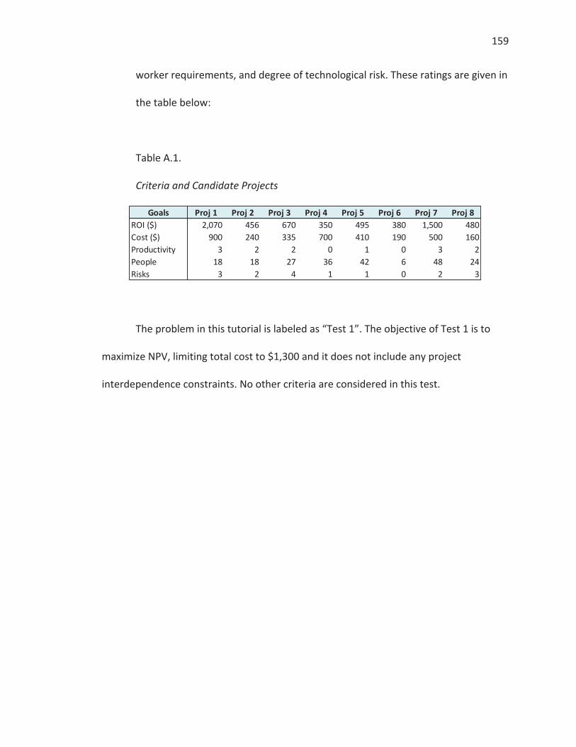
159
worker requirements, and degree of technological risk. These ratings are given in
the table below:
Table A.1.
Criteria and Candidate Projects
The problem in this tutorial is labeled as “Test 1”. The objective of Test 1 is to
maximize NPV, limiting total cost to $1,300 and it does not include any project
interdependence constraints. No other criteria are considered in this test.
Proj 1 Proj 2 Proj 3 Proj 4 Proj 5 Proj 6 Proj 7 Proj 82,070 456 670 350 495 380 1,500 480
900 240 335 700 410 190 500 1603 2 2 0 1 0 3 2
18 18 27 36 42 6 48 243 2 4 1 1 0 2 3
PeopleRisks
GoalsROI ($)Cost ($)Productivity

160
MAIN PAGE
Figure A.1 shows the screenshot with the initial page of the DSS (Main Page) which
contains a brief information of the DSS and se sequence to solve a problem.
Figure A.1 Screenshot of the Main Page of the DSS
On the right menu bar you have the following options:
Press “Model Setting” button to continue
Press “Quit” button if you want to Exit the DSS
Each time you select the “Main” button in the DSS you will be returned to this page
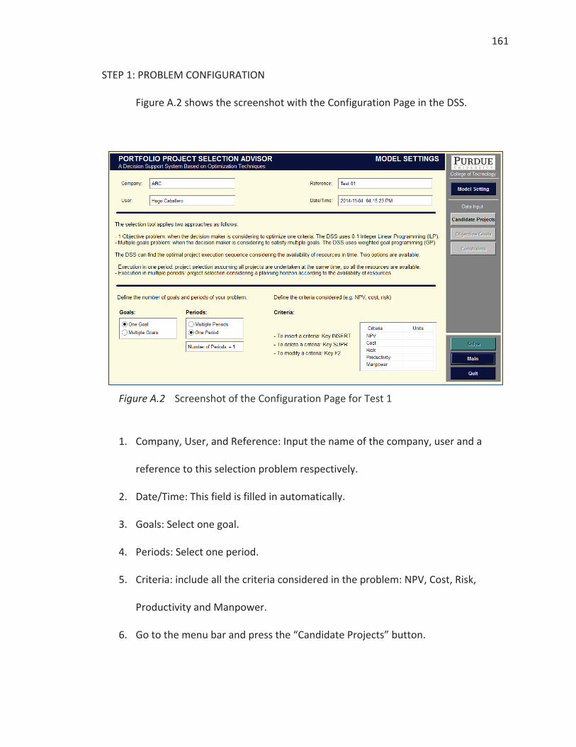
161
STEP 1: PROBLEM CONFIGURATION
Figure A.2 shows the screenshot with the Configuration Page in the DSS.
Figure A.2 Screenshot of the Configuration Page for Test 1
1. Company, User, and Reference: Input the name of the company, user and a
reference to this selection problem respectively.
2. Date/Time: This field is filled in automatically.
3. Goals: Select one goal.
4. Periods: Select one period.
5. Criteria: include all the criteria considered in the problem: NPV, Cost, Risk,
Productivity and Manpower.
6. Go to the menu bar and press the “Candidate Projects” button.
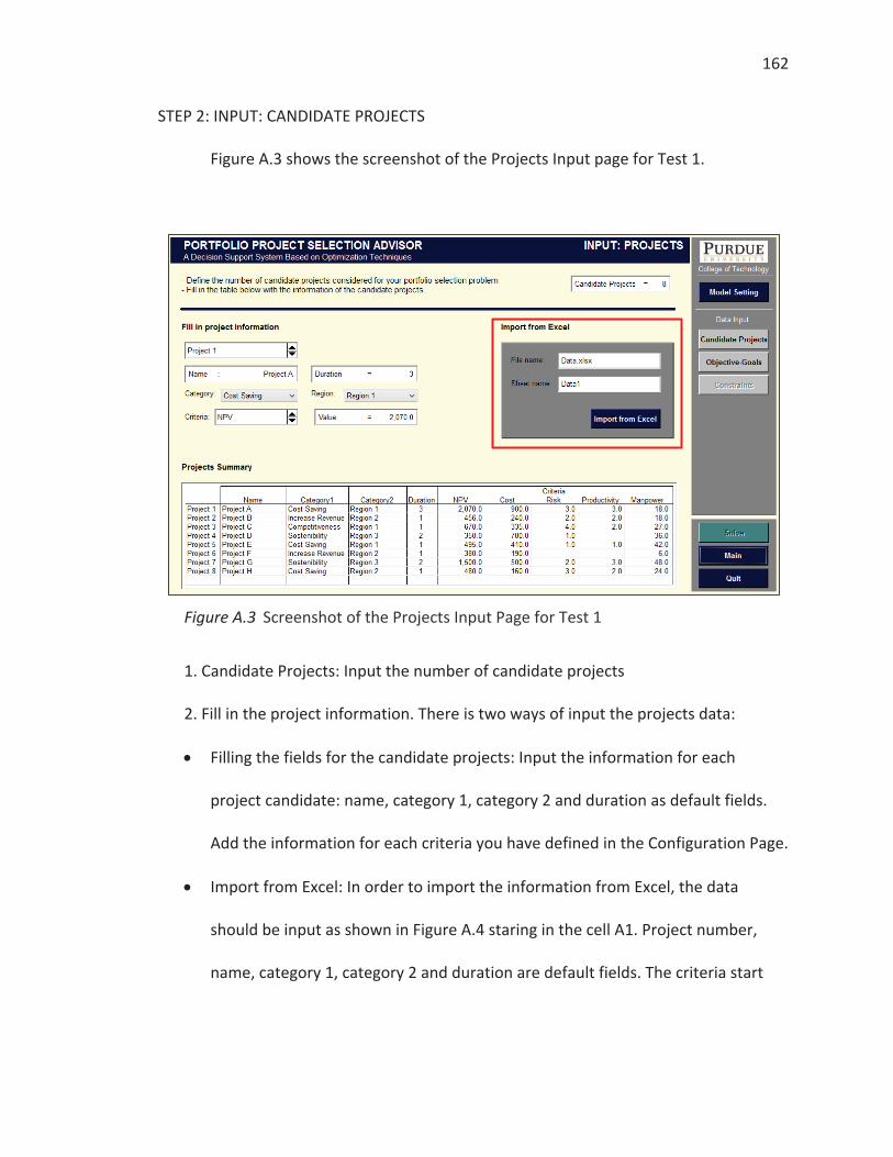
162
STEP 2: INPUT: CANDIDATE PROJECTS
Figure A.3 shows the screenshot of the Projects Input page for Test 1.
Figure A.3 Screenshot of the Projects Input Page for Test 1
1. Candidate Projects: Input the number of candidate projects
2. Fill in the project information. There is two ways of input the projects data:
Filling the fields for the candidate projects: Input the information for each
project candidate: name, category 1, category 2 and duration as default fields.
Add the information for each criteria you have defined in the Configuration Page.
Import from Excel: In order to import the information from Excel, the data
should be input as shown in Figure A.4 staring in the cell A1. Project number,
name, category 1, category 2 and duration are default fields. The criteria start
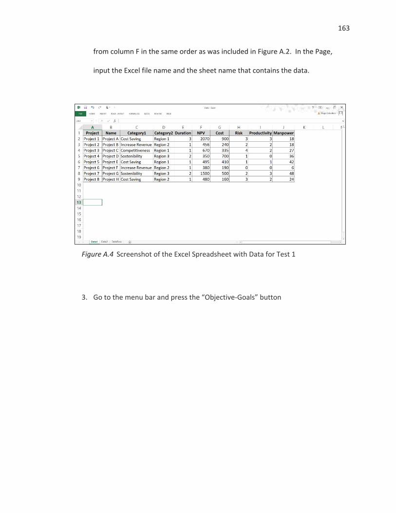
163
from column F in the same order as was included in Figure A.2. In the Page,
input the Excel file name and the sheet name that contains the data.
Figure A.4 Screenshot of the Excel Spreadsheet with Data for Test 1
3. Go to the menu bar and press the “Objective-Goals” button
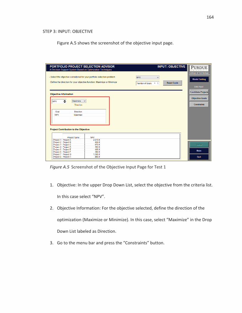
164
STEP 3: INPUT: OBJECTIVE
Figure A.5 shows the screenshot of the objective input page.
Figure A.5 Screenshot of the Objective Input Page for Test 1
1. Objective: In the upper Drop Down List, select the objective from the criteria list.
In this case select “NPV”.
2. Objective Information: For the objective selected, define the direction of the
optimization (Maximize or Minimize). In this case, select “Maximize” in the Drop
Down List labeled as Direction.
3. Go to the menu bar and press the “Constraints” button.
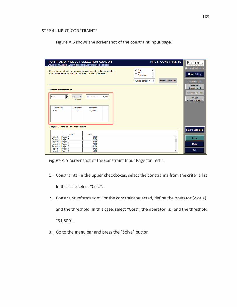
165
STEP 4: INPUT: CONSTRAINTS
Figure A.6 shows the screenshot of the constraint input page.
Figure A.6 Screenshot of the Constraint Input Page for Test 1
1. Constraints: In the upper checkboxes, select the constraints from the criteria list.
In this case select “Cost”.
2. Constraint Information: For the constraint selected, define the operator (≥ or ≤)
and the threshold. In this case, select “Cost”, the operator “≤” and the threshold
“$1,300”.
3. Go to the menu bar and press the “Solve” button

166
STEP 5: SOLUTION: PORTFOLIO
Figure A.7 shows the screenshot of the Solution-Portfolio page.
Figure A.7 Screenshot of the Solution Page for Test 1
In the Solution-Portfolio page can be found the following information:
Number of projects selected: 4
Number of candidate projects: 8
% of projects in the portfolio: 50%
The total NPV of the portfolio: $3,106
The total cost of the portfolio: $1,235
Project selected: projects 2, 3, 7 and 8
A bubble chart that shows in the x-axe the NPV and in the y-axe the cost. The
projects selected are the red bubbles and the projects not selected are blue

167
ones. The risk is by default the diameter of the bubble. It is possible display only
the set of projects selected or the set of projects no selected or using the check
box in the lower part of the bubble chart.
Projects information. You can select any project and the information of the
project NPV, cost and risk is shown.
Go to the menu bar and press the “Objective-Goals” button
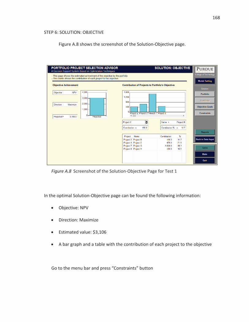
168
STEP 6: SOLUTION: OBJECTIVE
Figure A.8 shows the screenshot of the Solution-Objective page.
Figure A.8 Screenshot of the Solution-Objective Page for Test 1
In the optimal Solution-Objective page can be found the following information:
Objective: NPV
Direction: Maximize
Estimated value: $3,106
A bar graph and a table with the contribution of each project to the objective
Go to the menu bar and press “Constraints” button
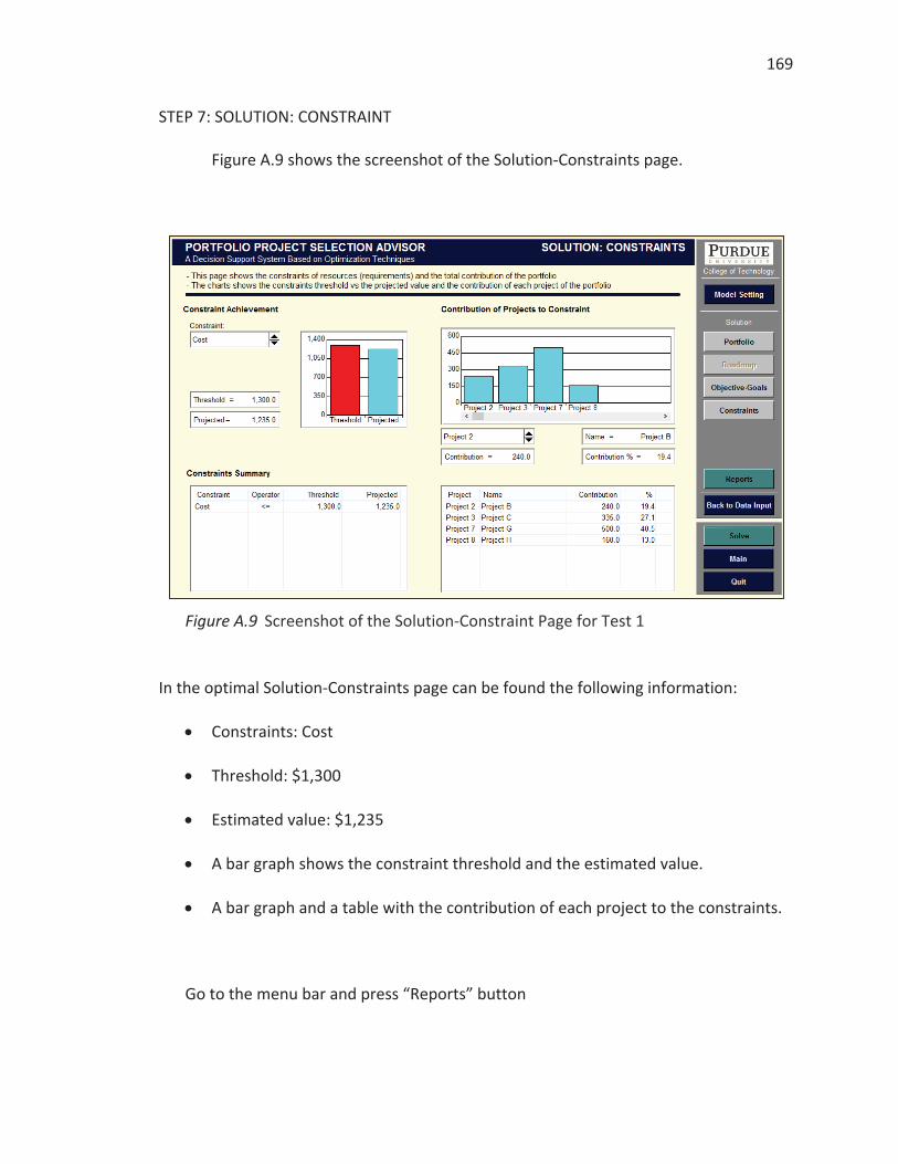
169
STEP 7: SOLUTION: CONSTRAINT
Figure A.9 shows the screenshot of the Solution-Constraints page.
Figure A.9 Screenshot of the Solution-Constraint Page for Test 1
In the optimal Solution-Constraints page can be found the following information:
Constraints: Cost
Threshold: $1,300
Estimated value: $1,235
A bar graph shows the constraint threshold and the estimated value.
A bar graph and a table with the contribution of each project to the constraints.
Go to the menu bar and press “Reports” button
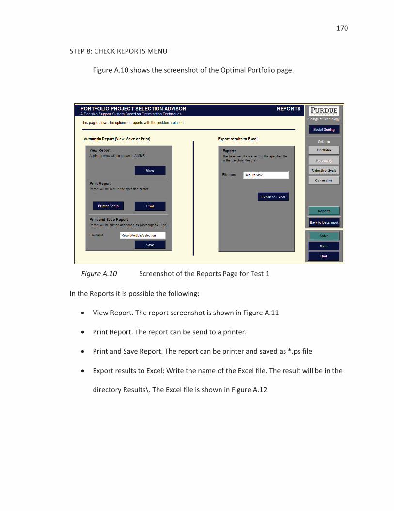
170
STEP 8: CHECK REPORTS MENU
Figure A.10 shows the screenshot of the Optimal Portfolio page.
Figure A.10 Screenshot of the Reports Page for Test 1
In the Reports it is possible the following:
View Report. The report screenshot is shown in Figure A.11
Print Report. The report can be send to a printer.
Print and Save Report. The report can be printer and saved as *.ps file
Export results to Excel: Write the name of the Excel file. The result will be in the
directory Results\. The Excel file is shown in Figure A.12

171
Figure A.11 Screenshot of the Report for Test 1
Figure A.12 Screenshot of the Excel File for Test 1

13
VITA
172
VITA
Hugo was born in 1974 in to Guido and Blanca de Caballero in Barranquilla,
Colombia, and has a younger sister, Idania Carolina.
Hugo received his Bachelor of Science degree in Mechanical Engineering from
Universidad del Norte in Barranquilla, Colombia. Upon graduation he joined the
Cummins distributor in Colombia as service engineer. After a couple years Hugo
received his MS in Mechanical Engineering from Universidad de los Andes in Bogota,
Colombia and then returned to the Cummins distributor as service manager. After three
years Hugo joined to Cementos Argos in Colombia as a project engineer. After six years
of experience leading projects in cement industry. This experience led to an interest in
the field of project and portfolio management and he applied to a Fulbright scholarship
for graduate studies at Purdue University. Hugo got a MS Industrial Engineering focus on
Operations Research in 2013 and a Ph.D. in Technology in 2014 working with Dr. Edie
Schmidt.
Hugo Caballero is married to Rita Jaramillo, a Ph.D. student in the Mechanical
Engineering department of Purdue University. Hugo and Rita are parents to an eight-
years-old daughter, Alejandra.