Project Report

Project #: TIC706.1-A Islanding Risk of Synchronous Generator Based

Distributed Generation Systems

Draft to be approved

Submitted

To

The CANMET Energy Technology Centre

Prepared

By

Wilsun Xu, Ph.D., P.Eng. Walmir Freitas, Ph.D. Dept. of Electrical and Computer Engineering

University of Alberta Edmonton, Alberta

Canada

Dept. of Electrical Energy Systems State University of Campinas

Campinas, Sao Paulo Brazil

March 31, 2008

2

DISCLAMER

This report is distributed for informational purposes and does not necessarily reflect the views of the Government of Canada nor constitute and endorsement of any commercial product or person. Neither Canada nor its ministers, officers, employees or agents makes any warranty in respect to this report or assumes any liability arising out of this report.

ACKNOWLEDGMENT Financial Support for this collaborative research project was provided in part by Natural Resources Canada through the Technology and Innovation Program as part of the Climate Action Plan for Canada. The authors wish to thank Mr. Sylvain Martel, the project manager, for his support and patience during the course of this project.

3

Table of Contents

Chapter 1: Introduction............................................................................................................................................7

Chapter 2: Anti-Islanding Protection for Distributed Generators............................................................................9

2.1 Electric Island Formed by Distributed Generators ........................................................................................9 2.2 Anti-islanding Protection Options for Synchronous DG .............................................................................11 2.3 Survey of Frequency-Based and Voltage-Based Relays..............................................................................12

Chapter 3: Operating Principles of Frequency and Voltage Based Relays............................................................14

3.1 Frequency and Voltage Relays ....................................................................................................................14 3.2 Rate of Change of Frequency Relay ............................................................................................................15 3.3 Vector Surge Relay......................................................................................................................................15

Chapter 4: Performance Characteristics of Frequency and Voltage Based Relays ...............................................17

4.1 The Concept of Anti-islanding Performance Curves ...................................................................................17 4.2 Performance Curves of the Frequency-Based Relays..................................................................................18

4.2.1 Performance Similarities of the Frequency and Vector Surge Relays .................................................19 4.2.2 Key Factors Affecting the Relay Performance ....................................................................................19 4.2.3 Equations to Predict Relay Performance .............................................................................................23 4.2.4 Limitations of Frequency (and Vector Surge) Relay ...........................................................................24 4.2.5 Limitation of the ROCOF Relay..........................................................................................................26

4.3 Performance Curves of the Voltage Relay...................................................................................................27 4.3.1 Key Factors Affecting the Relay Performance ....................................................................................28 4.3.2 Limitations of Voltage Relay...............................................................................................................30

Chapter 5: Non-Detection Zones of Combined Frequency and Voltage relays.....................................................32

5.1 The Concept of 2D Non-Detection Zone in PQ Plane.................................................................................32 5.2 Non-detection Zone of the Frequency Relay ...............................................................................................33 5.3 Non-detection Zone of the Voltage Relay ...................................................................................................34 5.4 Non-Detection Zone of Combined Frequency and Voltage Relays.............................................................35

Chapter 6: The Risk of Island Formation ..............................................................................................................38

6.1 The Concept of Islanding Risk ....................................................................................................................38 6.2 Survey of Islanding Risk Research ..............................................................................................................41 6.3 Strategy of the Proposed Work....................................................................................................................43

Chapter 7: Assessing the Risk of Islanding ...........................................................................................................46

7.1 The Basic Idea .............................................................................................................................................46 7.2 General Procedure for Risk Assessment......................................................................................................47 7.3 Modelling of the Non-Detection Zones .......................................................................................................53

Chapter 8: Characteristics of Islanding Risks........................................................................................................56

8.1 Description of the Study Case .....................................................................................................................56 8.2 Validation Study Results .............................................................................................................................58 8.3 Sensitivity Study Results .............................................................................................................................60

8.3.1 Types of Relays ...................................................................................................................................62 8.3.2 Relay Settings ......................................................................................................................................64 8.3.3 Generation Level .................................................................................................................................67

4

8.3.4 Generator Size .....................................................................................................................................70 8.3.5 Required Detection Time.....................................................................................................................73 8.3.6 Time Delay Relay Operation ...............................................................................................................76 8.3.7 Type of Loads ......................................................................................................................................79

8.4 The Worst Case Scenario.............................................................................................................................82 8.5 Summary and Recommended Procedures for Risk Assessment..................................................................84

Chapter 9: Conclusions..........................................................................................................................................86

Chapter 10: References............................................................................................................................................89

Appendix A: Methods FOR DeterminING Relay Performance Curves................................................................91

A.1 Simulation System.......................................................................................................................................91 A.2 Relay Models ...............................................................................................................................................91 A.3 Simulation and Analytical Studies...............................................................................................................93 A.4 Simulation Study of 2D Non-Detection Zone..............................................................................................94

Appendix B. Determination of Non-detection zones ............................................................................................96

Appendix C: Risk assessment Using Dynamic Simulations ...............................................................................100

Appendix D: Risk Assessment for systems with Constant Impedance Loads.....................................................102

Appendix E: Example of Time Domain Simulation Results .....................................................................................106

E.1. Simulation Results .........................................................................................................................................107

5

Executive Summary

This report presents the anti-islanding performance characteristics of both frequency-based and voltage-based relays when they are applied to synchronous distributed generators. It also provides methods for determining the risk levels of undetected islanding formation when these relays are used.

Anti-islanding protection has become an important requirement for distributed generation applications. A common industry practice to address the anti-islanding requirement is to determine if simple and low cost frequency-based and voltage-based relays are sufficient for a DG installation proposal. If it is not sufficient, more costly and advanced protection schemes are then considered. However, there have been no methods available for utility engineers to conduct the assessment on the applicability of the frequency/voltage based relays for synchronous distributed generators. This project is conducted to fill in this knowledge gap. The goal is to equip Canadian DG industry with techniques and tools for synchronous DG interconnection studies, thereby reducing the technical barrier for DG installation. The main results of this project are summarized here.

• The anti-islanding performance of individual relays can be characterized using detection-time versus power-mismatch (or power-imbalance) curves. Detection time is the time needed for a given relay to conclude that an island has formed. Power-mismatch is the power deficit or surplus of the island at the instant of island formation. Research results obtained by this project show that the frequency-based relays are sensitive to active power imbalance and the voltage-based relays are sensitive to reactive power imbalance. If the power imbalance is less than 10% to 20%, the relays may not be able to detect the island formation within typical required time.

• When both frequency-based relays and voltage-based relays are applied together, a non-detection zone can be established. A non-detection zone (NDZ) is the active and reactive power mismatch levels below which the combined relay schemes cannot detect island formation within an acceptable time delay. The NDZ is highly influenced by the load characteristics in the island. Study results show that the following equation can be used to estimate the typical size of the non-detection zone

%16'%36%8'%8

<Δ<−<Δ<−

QP

where QPP Δ−Δ=Δ 5.0866.0' and QPQ Δ+Δ=Δ 866.05.0' , ΔP and ΔQ are the power mismatch levels of the island.

• In this report, the risk of islanding formation is defined as the probability of a DG-containing distribution system entering the non-detection zones created by the frequency

6

and voltage based anti-islanding devices. Due to the wide variety of synchronous DG interconnection scenarios and distribution feeder configurations, it is not possible to provide typical risk values of island formation. This project therefore develops a practical risk assessment method for use by utility engineers. The method uses relay NDZ characteristics, feeder configuration, load profile and DG generation schedule as input and calculates the probability of the DG system entering the non-detection zones over a specified period such as one day or one week.

• Case studies using the proposed method revealed a few general characteristics of islanding risks associated with the frequency and voltage based relays. When increasing the required detection time from 500 ms to 1000 ms or 1500 ms, these relays can be quite effective in reducing the risk level of island formation. Time delay settings of the relays can increase the risk level if short detection time is required. The load characteristics can influence the risk of islanding significantly. The most conservative situations, which lead to higher risk levels, are related to both constant impedance and constant power loads. As the load characteristics of a distribution feeder is hardly known, worst cases that involve both types of load models should be used in the risk assessment.

7

CHAPTER 1: INTRODUCTION

Distributed generation (DG) has recently gained a lot of momentum due to market deregulation and environmental concerns. An important requirement to interconnect a DG to power distribution systems is the capability of the generator to detect island conditions. Islanding occurs when a portion of the distribution system becomes electrically isolated from the remainder of the power system, yet continues to be energized by distributed generators. Failure to trip islanded generators can lead to a number of problems to the generators and the connected loads. The current industry practice is to disconnect all distributed generators immediately after the occurrence of islands. Typically, a distributed generator should be disconnected within 100 to 2000 ms after loss of main supply [1,2,3].

To achieve such a goal, each distributed generator must be equipped with an islanding detection device, which is also called anti-islanding device. The most common devices used for this purpose are the under/over frequency relays, under/over voltage relays and their variations. These relays have very low cost and are widely available. They are the first choice for anti-islanding protection. The frequency-based relays operate on the principle that if the generation and load have a large mismatch in an island the frequency of the island will drift. One can therefore detect the islanding condition by checking the amount and rate of frequency change. The voltage relay is based on the understanding that the voltage in an island will also drift because of reactive power imbalance.

Unfortunately, these relays are not 100 percent reliable due to their inherent limitations. If the active/reactive power imbalance in an island is small, it will take some time for the islanded system to exhibit detectable frequency or voltage change. As a result, the relays will not be able to provide anti-islanding protection in a timely manner. The corresponding system operating conditions are called non-detection zones of the relays. In view of the significant cost advantages of the frequency and voltage relays, it has becomes imperative for utility companies and DG owners to understand the characteristics of the non-detection zones and the associated risks. The information will greatly facilitate the selection of DG protection schemes and has the potential to achieve significant cost-savings for the DG owners.

The objective of this report is to present our research results on the anti-islanding performance characteristics of both frequency-based and voltage-based relays when they are applied to synchronous distributed generators. Over the past 5 to 10 years, non-detection zone research has been concentrated on inverter-based DGs due to the popularity of photovoltaic power supplies. For example, the International Energy Agency (IEA) sponsored a systematic investigation on the subject [4,5,6]. The results have clarified a lot of concerns on the risks associated with inverter-based DGs back feeding an island. In comparison, no similar work has been done for the synchronous machine based DGs. In fact, due to its relatively large size and

8

lack of flexibility in output control, the synchronous DGs have become the most challenging type to establish adequate anti-islanding protection [7].

This project is conducted to address the non-detection zone issues associated with the synchronous DGs. The goal is to equip Canadian DG industry with sufficient information so that it can assess the applicability of the frequency/voltage relays and associated risks for various synchronous DG interconnection projects. This report is organized in three parts:

• The first part, consisting of Chapters 2 and 3, discusses the nature and requirements of anti-islanding protection. The frequency and voltage relays are introduced and their operating principles are explained.

• The second part, consisting of Chapters 4 and 5, presents the anti-islanding protection characteristics of various frequency-based and voltage-based relays. Chapter 4 focuses on the detection-time versus power mismatch curves of the relays. These curves show how long it will take for a relay to operate for a given power mismatch condition. Chapter 5 presents the non-detection zones of the relays.

• The third part, consisting of Chapters 6, 7 and 8, investigates the risks caused by the non-detection zones. The risk of islanding formulation is essentially the probability of a DG-containing distribution system entering the non-detection zones created by the anti-islanding devices. A practical risk assessment method is presented to determine if the frequency and voltage relays can be used with confidence.

9

CHAPTER 2: ANTI-ISLANDING PROTECTION FOR DISTRIBUTED GENERATORS

Anti-islanding capability is an important requirement for distributed generators. It refers to the capability of a distributed generator to detect if it operates in an islanded system and to disconnect itself from the system in a timely fashion. This chapter reviews the background information on the DG anti-islanding protection. Two most common anti-islanding options for synchronous machine based distributed generators, frequency-based and voltage-based relays, are discussed.

2.1 Electric Island Formed by Distributed Generators

A typical power distribution system in North America is shown in Figure 2.1. The substation steps down transmission voltage into distribution voltage and is the sending end of several distribution feeders. One of the feeders is shown in detail. There are many customer connection points in the feeder. Large distributed generators are typically connected to the primary feeders (DG1 and DG2). These are typically synchronous and induction generators at present. Small distributed generators such as inverter based PV systems are connected to the low voltage secondary feeders (DG3).

DG2

A

B

130kV

25kV

Substation 1

DG1

C

D

DG3120V

F

Island

Figure 2.1: Typical distribution system with distributed generators.

An island situation occurs, for example, when recloser C opens. DG1 will feed into the resultant island in this case. The most common cause for a recloser to open is a fault in the

10

downstream of the recloser. A recloser is designed to open and re-close two to three times within a few seconds. The intention is to re-connect the downstream system automatically if the fault clears by itself. In this way, temporary faults will not result in the loss of downstream customers. An island situation could also happen when the fuse at point F melts. In this case, the inverter based DG will feed the local loads, forming a small islanded power system.

The island is an unregulated power system. Its behaviour is unpredictable due to the power mismatch between the load and generation and the lack of voltage and frequency control. The main concerns associated with such islanded systems are:

• The voltage and frequency provided to the customers in the islanded system can vary significantly if the distributed generators do not provide regulation of voltage and frequency and do not have protective relaying to limit voltage and frequency excursions. Since the supply utility is no longer controlling the voltage and frequency, the islanding situation could result in damages to customer equipment. Although the supply utility has no control over the situation, it may still be found liable for the consequences.

• Islanding may create a hazard for utility line-workers or the public by causing a line to remain energized that may be assumed to be disconnected from all energy sources.

• The distributed generators in the island could be damaged when the island is reconnected to the supply system. This is because the generators are likely not in synchronism with the system at the instant of reconnection. Such out-of-phase reclosing can inject a large current to the generators. It may also result in re-tripping in the supply system.

• Islanding may interfere with the manual or automatic restoration of normal service for the neighboring customers.

The current industry practice is to disconnect all DGs immediately so that the entire feeder becomes de-energized [1,2,3]. It prevents equipment damage and eliminates safety hazards. This calls for a reliable and speedy detection of islanding conditions. The basic requirements for a successful detection are:

• The scheme should work for any possible formations of islands. Note that there could be multiple switchers, reclosers and fuses between a distributed generator and the supply substation. Opening of any one of the devices will form an island. Since each island formation can have different mixture of loads and distributed generators, the behaviour of each island can be quite different. A reliable anti-islanding scheme must work for all possible islanding scenarios.

• The scheme should detect islanding conditions within the required time frame. The main constraint here is to prevent out-of-phase reclosing of the distributed generators. A

11

recloser is typically programmed to reenergize its downstream system after about 0.5 to 1 second delay. Ideally, the anti-islanding scheme must trip its DG before the reclosing takes place.

The above goal is achieved by equipping each DG with an anti-islanding protection capability – each DG must be able to detect if it is islanded and to disconnect itself automatically from the system when islanding occurs. In response to the requirements, many anti-islanding techniques have been proposed and a number of them have been implemented in actual DG projects [4] or incorporated into some of the DG controller. Reference [7] provides a comprehensive review of various anti-islanding techniques. The work of reference [7] further revealed that anti-islanding protection for synchronous distributed generators is the primary concern for Canadian DG industry and supply utilities.

2.2 Anti-islanding Protection Options for Synchronous DG

Synchronous distributed generators use synchronous machine as the energy converter. The generators are typically connected to the primary feeder. Their sizes can go as high as 30MW. Synchronous generators are highly capable of sustaining an island. Due to its large power rating, options are limited to control the generators for the purpose of facilitating islanding detection. As a result, anti-islanding protection for synchronous generators has emerged as one of the most challenging tasks facing the DG industry.

Methods available for synchronous DG anti-islanding protection can be broadly classified into two types according to their working principles. The first type consists of communication-based schemes. It uses telecommunication means to alert and trip DGs when islands are formed. The transfer trip scheme well known to utility companies belongs to this type. The telecomm-based schemes can be quite expensive and could render a DG project economically unattractive.

The second type is to rely on the voltage and current signals available at the DG site. An islanding condition is detected if indices derived from the signals exceed certain thresholds. Frequency-based and voltage-based anti-islanding relays are representative examples of such schemes. The relays trip a DG if the frequency or voltage measured at the DG location drifts outside pre-established safe operation boundaries. Due to their low cost and simplicity, frequency-based and voltage-based relays are the first choice by the DG owners to provide anti-islanding protection for synchronous DGs.

The frequency-based schemes are the most widely used scheme for anti-islanding protection involving synchronous generators. It is known if the generation and load have a large mismatch in a power system, the frequency of the system will change. In view of the fact that the frequency is constant when the feeder is connected to the transmission system, it is possible to detect the islanding condition by checking the amount and rate of frequency change. Several

12

commercial products based on this idea have been developed and are available for use at present. They can be classified into the following three types [8]:

• Over/under frequency relay, which is called frequency relay in this report;

• Rate of change of frequency relay, which is called ROCOF relay in this report; and

• Vector surge (jump or shift) relay, which is called VSR relay in this report.

There is only one type of voltage-based relays commercially available for anti-islanding protection. It is the over/under voltage relay and is called voltage relay in this report. The relay operates on the principle of reactive power mismatch in an island. Excessive reactive power will drive up the system voltage and deficit reactive power will result in voltage decline. By determining the level of voltage at the DG terminal, it is possible to detect islanding conditions that cannot be detected by frequency-based relays. Note that a voltage relay is needed for other protection purposes in a DG installation. For example, it is used to prevent over-voltage stress to the DG unit. A voltage relay is, therefore, always available in a DG installation and can be utilised to support islanding detection at no extra cost.

As the frequency-based and voltage-based relays are the first choice for anti-islanding protection, it becomes important to understand their performance characteristics and limitations. Such information will help DG owners and supply utilities to determine if the relays can perform the required anti-islanding task reliably. Other anti-islanding options may be considered only after it is determined that the frequency and voltage-based relays are unable to meet the requirements. One of the main objectives of this project is to provide methods and data to help DG owners and utility engineers to assess the applicability of the common frequency-based and voltage-based relays for specific synchronous DG installations.

2.3 Survey of Frequency-Based and Voltage-Based Relays

The frequency and voltage relays are common relays found in various power system protection applications. As a result, many relay manufacturers have the products. Because of their commonality, this project only surveyed products that are specifically designed for DG anti-islanding protection. Table 2.1 summarises the findings. It is important to note that this is not an exhaustive survey, but rather a sample of what is typically available in the market.

It can be seen that anti-islanding products based on the principle of frequency or voltage variation detection are widely available. This is an indication that frequency- and voltage-based relays are the common choice for anti-islanding protection. The survey found that the relay prices vary from $1000 to $5000. The high priced relays include other DG protection functions. Although the products are widely available, it is not clear how reliable they are in providing anti-

13

islanding protection and what are the performance characteristics of the different relays. Chapter 4 will provide answers to these and other related questions.

Table 2.1: Sample manufacturers and products of frequency-based anti-islanding relays.

Manufacturer Product Name Principle SEL (USA) DG interconnection Relay: SEL-547 • Under/over frequency

• Under/over voltage Basler Electric (USA) BE1-IPS100 Intertie Protection System • Under/over frequency

• Under/over voltage • ROCOF

Cooper Power Systems (USA)

UM30SV Vector jump/islanding relay • VSR • Under/over frequency • Under/over voltage

Woodward (USA) MFR-11/G59 Multi Function Mains Protection

• ROCOF • VSR

Meidensha Corp. (Japan) Loss of Mains relay • ROCOF Sepam (UK) Sepam 1000+ • ROCOF Crompton Instruments (UK) 256-ROCL Vector Shift and ROCOF relay • VSR

• ROCOF Megacon (UK) KCG592 Loss of Mains Relay • ROCOF

• VSR ABB Oy (Finland) SPAF 140C Frequency Relay • Under/over frequency

• ROCOF DEIF A/S (Denmark) 1) G59 Protection relay package

2) LMR-122D Loss of Mains Relay

• VSR • ROCOF • Over/under frequency • Over/under voltage

14

CHAPTER 3: OPERATING PRINCIPLES OF FREQUENCY AND VOLTAGE BASED RELAYS

This chapter presents the principles of the frequency and voltage based relays. Differences and similarities among the three types of frequency-based relays are discussed. The operating principles form the basis to determine the performance characteristics of the relays for anti-islanding applications.

3.1 Frequency and Voltage Relays

Measuring frequency and voltage is one of the basic functions performed by modern microprocessor relays. To measure the frequency, a voltage signal supplied from a PT (potential transformer) is first filtered using a band-pass filter. This operation reduces the impact of waveform distortion on the measurement accuracy. The frequency is determined by measuring the time between the zero crossings of the filtered waveform [9]. Each cycle of the waveform yield one frequency value. Typically, the relay works on a moving average of the per-cycle frequencies. The number of cycles used for the moving average calculation varies from 3 to 30 cycles and is selectable by users. When the calculation is based on three cycles, the measurement response time will be short and, consequently, the trip time as well. On the other hand, when thirty cycles are used the response time will be long, but the effect of the noise possibly occurring in the signal will be small.

The RMS magnitude of the voltage signal is measured using the following equation [9]:

∑=

=N

iirms v

NV

1

21 (1)

where N is number of samples per cycle and vi is the sample value. As a result, each cycle yields one voltage magnitude value. A moving average is also used to produce a voltage value that is used to compare with a user-specified threshold and thereby activate the relay.

Both the frequency and voltage relays have at least one time delay setting in addition to magnitude threshold settings. A delayed activation is often needed to avoid false trips caused by system conditions outside the protective scope of the relays. As an example, typical frequency relay settings to protect a generator from over speeding are 61Hz with an 1.0 second delay and 63Hz with a 0.3 second delay. For the DG applications, the DG interconnection guide of Alberta specifies 59.5 Hz as the under frequency threshold and 60.5Hz as the over-frequency threshold. A DG shall be tripped within 0.5 seconds if either of the thresholds is exceeded.

15

3.2 Rate of Change of Frequency Relay

The ROCOF relay calculates the rate of change of frequency (df/dt) using two successive moving-average frequency values. The moving average is based on, for example, 3 cycles of voltage waveform. This window size is typically built into the relay and it cannot be easily changed by users. The relay activates when the rate of change of frequency is higher than a user-specified threshold and after a user-specified time delay. Typical ROCOF relay settings for 60 Hz systems are between 0.5 Hz/s and 2.50 Hz/s. Another important characteristic available in the ROCOF relay is a blocking function according to minimum generator terminal voltage. If the terminal voltage drops below an adjustable level Vmin, the trip signal from the ROCOF relay is blocked. This is to avoid, for example, the actuation of the ROCOF relay during generator start-up or short-circuit faults.

3.3 Vector Surge Relay

The principle of the VSR relay can be understood from Figure 3.1 where a synchronous generator equipped with the relay interconnects to a distribution network. There is a voltage drop ΔV between the terminal voltage VT and the generator internal voltage EI due to the generator current ISG passing through the generator reactance Xd. Consequently, a displacement angle δ exists between the terminal voltage and the generator internal voltage. The phasor diagram is shown in Figure 3.1(a). If the circuit breaker CB opens, due to a fault for example, the system composed by the generator and the load L becomes islanded. The synchronous machine begins to feed a larger (or smaller) load, which makes it to decelerate (or accelerate). Consequently, the angular difference between VT and EI is suddenly increased (or decreased) and the terminal voltage phasor changes its direction, as shown in Figure 3.1(b). Viewing such a phenomenon in the time domain, we can notice that the instantaneous value of the terminal voltage jumps to another value and the phase position changes, as depicted in Figure 3.1, where the point A indicates the islanding instant. Additionally, the frequency of the terminal voltage also changes. This behaviour of the terminal voltage is called vector surge or vector shift. The vector surge relay is based on such a phenomenon.

L

Xd

TVIE

SGI CB powergrid

SYSIVΔ VSR

δ Δδ

EI VT V’T

ΔV ΔV’

(a) (b)

EI

(a) Network diagram. (b) Voltage phasor (‘vector’) diagram.

Figure 3.1: The phenomenon of ‘vector surge’ or ‘vector shift’.

16

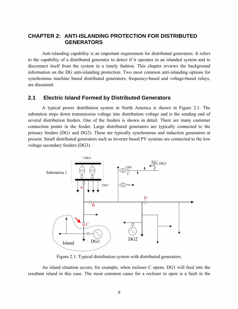
The vector surge relays available in the market measure the duration of an electrical cycle and start a new measurement at each positive-going zero crossing of the terminal voltage. The cycle whose duration is to be measured is compared with the previous cycle (called reference cycle). In an islanding situation, the cycle duration is either shorter or longer, depending on if there is excess or deficit of power in the islanded system. This variation of the cycle duration represents the variation of the terminal voltage angle Δδ. If the variation of the terminal voltage angle exceeds a pre-determined threshold α, a trip signal is immediately sent to the circuit breaker. Usually, vector surge relays allow this threshold to be adjusted in the range from 2 to 20 degrees. The vector surge relay also has a minimum terminal voltage triggered blocking function. If the terminal voltage drops below an adjustable level threshold Vmin, the trip signal from the vector surge relay is blocked.

Δt ∝ Δθ Δt ∝ Δθ

reference

measuredwaveform

A

V(t)

time new reference

Figure 3.2: Measurement of the vector surge or shift.

It can be shown that the shift, Δθ, is an indirect measurement of the waveform frequency. As a result, this type of relay is expected to have a performance characteristic similar to that of the frequency relay.

17

CHAPTER 4: PERFORMANCE CHARACTERISTICS OF FREQUENCY AND VOLTAGE BASED RELAYS

The previous chapters have shown that at least four types of simple relays are available for DG anti-islanding protection. It becomes necessary to understand the performance characteristics of these relays. This chapter introduces the concept of performance curves for the relays and discusses the key factors that can affect the relay performance. Furthermore, the concept of a two-dimensional non-detection zone is presented for applications where both frequency and voltage-based relays are used to form a composite anti-islanding protection scheme.

4.1 The Concept of Anti-islanding Performance Curves

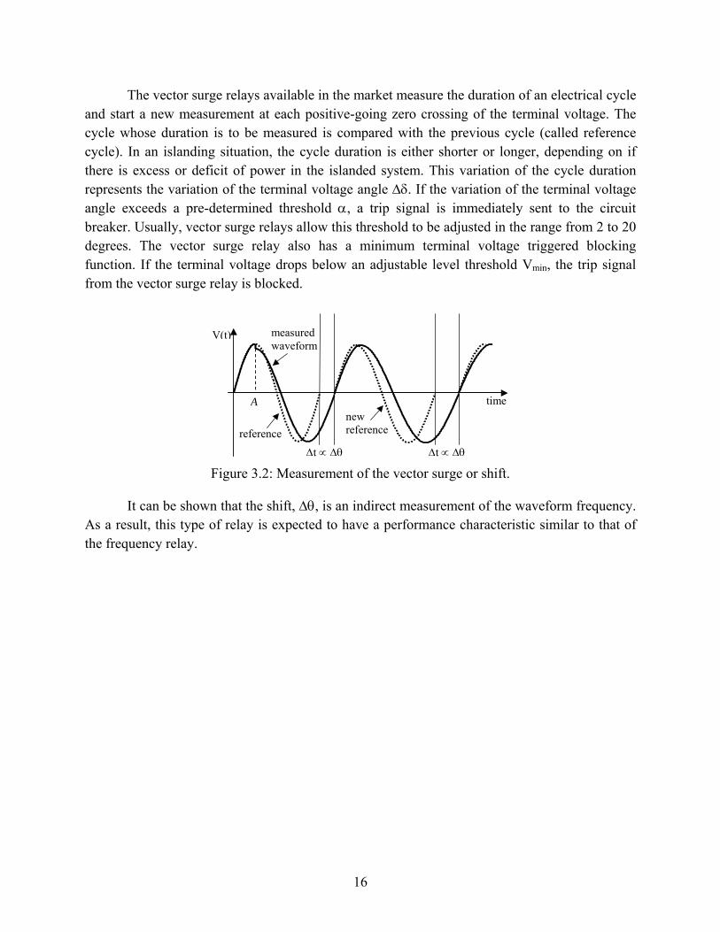
The frequency-based relays work on the principle of active power imbalance in an island. A large power imbalance will cause fast deviation of frequency in the island and it will take less time to detect the islanding condition. An approach to evaluate the performance of frequency-based anti-islanding relays is, therefore, to understand the relationship between the tripping (or detection) time and power imbalance (or mismatch). This relationship can be represented with a detection-time versus power-mismatch curve as shown in Figure 4.1.

0

100

200

300

400

500

0 0.1 0.2 0.3 0.4 0.5 0.6 0.7 0.8 0.9 1 Active power imbalance (pu)

Det

ectio

n tim

e (m

s)

5 degrees10 degrees 15 degrees

Non-detection zone

Figure 4.1: Typical detection-time versus power-imbalance characteristics of frequency-based relays.

The figure uses the vector surge relay as an example. There are three curves each representing a different setting of the VSR. The x-axis is the power mismatch level of the islanded system referred to the rated MVA of the DG. The y-axis is the time needed by the relay

18

to operate, since it takes time for the islanded system to exhibit detectable frequency variation. If it is required to trip the distributed generator within 300ms after islanding, one can draw a horizontal line of 300ms. The intersection of this line with the relay curve of 10 degrees gives 33% power mismatch level. If an islanded system has a power imbalance greater than 33%, it would take less than 300ms to detect the islanding condition. So the relay can be used with confidence. One the other hand, the relay will take longer than 300ms to operate if the power imbalance level is less than 33%. Consequently, the relay is not suitable for such cases. The 33% power mismatch level is called the critical power mismatch. The power-mismatch level below the critical power mismatch represents a (one-dimensional) non-detection zone of the relay.

Similar performance curves can be developed for the voltage relay. Since voltage is sensitive to reactive power, the performance curves for voltage relays are represented as detection-time versus reactive-power-mismatch curves. Details are shown in Section 4.3. Methods to determine the performance curves for the relays are presented in Appendix A.

4.2 Performance Curves of the Frequency-Based Relays

Sample detection-time versus power-mismatch curves for the frequency, ROCOF and vector surge relays are shown in Figure 4.2 for islands consisting of one synchronous generator. It can be seen that the VSR and frequency relays have similar performance. The ROCOF relay has the best performance since its non-detection zone is the smallest. The results also reveal that a non-detection zone of 10% to 30% power mismatch exists for all relay types. Reducing the trip threshold can reduce the non-detection zone. This approach, however, could make the relays too sensitive, resulting in more opportunities of nuisance trips. Because of this reason, the ROCOF relay is more prone to nuisance trips.

0 0.2 0.4 0.6 0.8 1 0 100 200 300 400 500 600 700 800 900

1000

Active power imbalance (pu)

Det

ectio

n tim

e (m

s)

Frequency relay: ± 1.0 HzFrequency relay: ± 1.5 HzFrequency relay: ± 2.0 HzVector surge relay: 6 degreesVector surge relay: 9 degreesVector surge relay: 12 degreesROCOF relay: 0.5 Hz/sROCOF relay: 1.5 Hz/sROCOF relay: 2.5 Hz/s

Figure 4.2: Characteristics of three types of frequency-based anti-islanding relays.

19

4.2.1 Performance Similarities of the Frequency and Vector Surge Relays

Figure 4.2 has revealed that the frequency relay and the vector surge relay have almost identical performance characteristics. Extensive research results show that this is not a coincidence. In this section, a comparison between the anti-islanding capability of the frequency and vector surge relays is carried out in detail.

In a 60 Hz system, 1 Hz corresponds to 6 electrical degrees. Therefore, a frequency relay setting of 0.5 Hz can be compared with a VSR relay setting of 3 degrees and so on. The critical power imbalances for typical relay settings and for a required detection time of 300, 500 or 700 ms are presented in Table 4.1. In this table, the power mismatches are presented in percentage of the generator MVA rating; the frequency relay is referred as FR and the vector surge relay as VSR. It can be noted that both relays give very similar critical power imbalances. This further confirms the conclusion drawn earlier. The significance of this finding is the following: The vector surge relay does not offer additional advantages over the frequency relay for anti-islanding protection. As a result, there is no need to install a dedicated VSR for anti-islanding application because a frequency relay, which is normally required for any DG installation, is as effective as the vector surge relay for anti-islanding application. The savings can be quite attractive for small distributed generators and the resultant protection system will be much simpler.

Because the vector surge relay has almost the same performance characteristic as that of the frequency relay, the VSR relay will not be signalled out for separate analysis and discussion in the subsequent chapters. As a result, we will only focus on two types of relays, the frequency relay and the ROCOF relay in the rest of this report.

Table 4.1: Comparison of the critical power mismatch of the frequency and VSR relays.

Detection time 300 ms 500 ms 700 ms Settings

FR / VSR FR VSR FR VSR FR VSR

0.5 Hz / 3o 20.6% 19.2% 15.1% 14.5% 21.0% 11.8% 1.0 Hz / 6o 31.5% 27.7% 20.9% 19.6% 16.2% 15.6% 1.5 Hz / 9o 42.2% 36.1% 26.6% 24.3% 20.2% 19.2% 2.0 Hz / 12o 53.0% 43.3% 32.3% 29.9% 24.4% 23.0% 2.5 Hz / 15o 63.9% 52.9% 37.9% 34.5% 28.3% 26.9%

4.2.2 Key Factors Affecting the Relay Performance

It is important to note that Figure 4.2 is an illustration of the typical characteristics of frequency-based relays. A number of factors can affect the curves. Research results show that the following factors have significant impact on the relay performance:

20

• Inertia constant of the distributed generator; • Voltage dependency of the feeder loads; and • The mode of generator excitation control (if the load is not constant power type)

The impact of DG inertia constant, H, can be seen from Figure 4.3(a). A larger H constant will lead to a larger critical power imbalance for the same relay setting. This is understandable since it takes longer time to cause a frequency deviation for DGs with a larger rotor inertia constant. In order to avoid the use of multiple relay curves for different H values, a normalised performance curve is proposed. For this curve, a normalised power mismatch value defined as:

HPPnormalized

Δ=Δ

(2)

is used as the x-axis value of the curve. As shown in Figure 4.3(b), the normalised curve is the same for different H constants. As a result, a single relay curve can be used to assess DG applications involving different DG sizes.

0 0.2 0.4 0.6 0.8 10 100 200 300 400 500 600 700 800 900

1000

Active power imbalance (pu)

Det

ectio

n tim

e (m

s)

H = 2.0 sH = 1.5 sH = 1.0 s

0 0.2 0.4 0.6 0.8 10

100

200

300

400

500

600

700

800

900

1000

Normalised active power imbalance (pu)

Det

ectio

n tim

e (m

s)

H = 2.0 sH = 1.5 sH = 1.0 s

(a) Performance curves for different H constant. (b) Normalised performance curves.

Figure 4.3: Impact of machine inertia constant on detection curves of a frequency relay.

The impact of voltage dependency of the feeder loads is illustrated in Figure 4.4. The constant power load model represents a load characteristic that is independent of voltage. The constant current model represents a load characteristic whose power consumption varies linearly with the supply voltage. The constant impedance model represents a load characteristic whose power consumption varies with the square of the supply voltage. Since the constant impedance load can create a larger power surplus or deficit in an islanded system if the system voltage changes a lot, its performance curves deviate from the constant power curve more significantly. As the load-voltage dependency characteristics of a distribution feeder is hardly known, we have

21

to rely on the constant power load curve as a reference to obtain a general understanding of the critical power mismatch of the relays.

0 0.2 0.4 0.6 0.8 10 100 200 300 400 500 600 700 800 900

1000

Active power imbalance (pu)

Det

ectio

n tim

e (m

s)

Constant power model Constant current model Constant impedance model

Deficit of active power Excess of active power

0 0.2 0.4 0.6 0.8 10

100

200

300

400

500

600

700

800

900

1000

Active power imbalance (pu)

Det

ectio

n tim

e (m

s)

Constant power model Constant current model Constant impedance model

Deficit of active power

Excess of active power

(a) Frequency relay (setting = ±1.5 Hz). (b) ROCOF Relay (Setting = 1.0 Hz/s).

(The reactive power is in deficit for both cases)

Figure 4.4: Impact of load to voltage dependency on the relay performance characteristics.

A distributed generator typically has two modes of controlling its excitation system. One is to maintain constant terminal voltage (voltage control mode) and the other is to maintain constant power factor (power factor control mode) [8]. The tripping time versus power imbalance curves for the two control modes are compared in Figure 4.5 for the frequency relay, assuming there is a shortage of electrical power after islanding and the load is constant impedance type. For the conditions of active and reactive power imbalances simulated in this section, it is found that the critical power imbalance is larger if the excitation system is controlled by power factor than by voltage. This is due to the different response of nodal voltages under different control mode. The voltage control mode will lead to less voltage change in the system. The power shortage in the island is therefore more than that associated with the power factor control mode, which leads to a larger power mismatch for the voltage control mode. So the voltage control mode can result in faster frequency drift and smaller critical power imbalance. For the same reason, the case in which there is excess of electrical power after islanding will result in a smaller critical power mismatch for the power factor control mode than for the voltage control mode. As a result, which mode has smaller non-detection zone is dependent on if the island has deficit or surplus of power. Further study shows that if the load is constant power type, there is no difference between the two control modes.

Research results showed that other factors such as feeder length and load power factors have little impact on the relay performance curves. If there are multiple DGs in an island, the frequency-based relays could interact with each other. This is because the tripping of one generator will change the power mismatch level in the island, which in turn affects the variation of system frequencies. The relay behaviours can be difficult to predict under such circumstance

22

[10]. Research results also show that the ROCOF relay can cause more nuisance trips than the vector surge relay. The main conclusions from such impact factor study can be summarised as follows:

0 0.2 0.4 0.6 0.8 1 0

100

200

300

400

500

600

700

800

900

1000

Active power imbalance (pu)

Det

ectio

n tim

e (m

s)

V control mode Q control mode

±1.0 Hz ±1.5 Hz ±2.0 Hz

Figure 4.5: Impact of DG excitation control modes.

• The voltage-dependency of the feeder loads has a significant impact on the relay performance curves. The load type also affects the performance indirectly through DG excitation modes. Since the load-to-voltage dependency is hard to quantify for a given distribution system and for different island formations, we recommend to use the relay curves obtained with the constant power load assumption as a reference. An approximate critical power mismatch level can be determined from the reference curve. A safe margin of 0.1 to 0.3 per-unit power mismatch may be added to critical power mismatch level to arrive at a conservative estimate of the non-detection zone.

• The DG inertia constant also has a significant impact on the performance curves. This factor can be taken into account by using H-constant normalised relay performance curves.

• The following factors do not have significant impact on the relay anti-islanding performance: feeder length, X/R ratio of the feeder impedance, load power factor, and reactive power imbalance of the island.

The reactive power mismatch in an island has some impact on the relay performance. This subject will be discussed in Chapter 5 where a two-dimensional non-detection zone will be introduced.

23

4.2.3 Equations to Predict Relay Performance

Equations to predict the performance of the frequency-based relays have been developed [10,11,12]. Mathematical models on which the equations are based are explained in Appendix A. For the frequency relay, the equation representing the relay performance under the constant power load condition has the following form:

τφφ+

Δ=

Δ=

)/(302

0 HPPfHtd

(3)

where td is the detection time; τ is the time used to compute the frequency value and run the relay algorithm.

From manufacturers catalogues this intrinsic delay is around 80 ms. H is the generator H constant; fo is the power system frequency (60 Hz in this report); φ is the relay setting, for example 0.5Hz; and ΔP is the power mismatch between load and generation in absolute per-unit value defined as ΔP=|(Pgen-Pload)/Pgen-rated |

For the ROCOF relay, the performance equation has the following form:

τβτβ +⎟⎟⎠

⎞⎜⎜⎝

⎛Δ

−−=+⎟⎟⎠

⎞⎜⎜⎝

⎛Δ

−−=)/(30

1ln21ln0 HP

TPf

HTt aad (4)

where β is the relay setting, for example, 1.2Hz/s; τ is the time used to compute the df/dt value and run the relay algorithm. From manufacturers catalogues this intrinsic delay is around 130 ms. Ta is the time constant of a low pass filter that models the averaging algorithm to estimate df/dt. Typical value of Ta is 100 ms (or 6 cycles);

For the vector surge relay, the performance equation is:

)2(2D))(2(

20

παπαω

−−−−

=KKtd

(5)

where )/30(22/ HPHPK o Δ=Δ= πω ; D = (2ω0K(α − π ))2 − 4K2(α − 2π)(ω0

2α + 2π2K); α is the relay setting in the unit of radian.

A set of general purpose curves to predict the relay performance is determined using the above equations and is shown in Figure 4.6. Note that the x-axis is the normalized power mismatch, defined as ΔPn=ΔP/H. Because of the normalization, the curves can be applied to generators of any size. References [10,11,12] further investigated empirical formulas for cases where the load is not a constant power type. Details can be found from the references.

24

0 0.2 0.4 0.6 0.8 10

100 200 300 400 500 600 700 800 900

1000

Normalised active power imbalance ( )

Det

ectio

n tim

e (m

s)

± 1.0 Hz± 1.5 Hz± 2.0 Hz

(a) Frequency relay.

0 0.1 0.2 0.3 0.4 0.50

100 200 300 400 500 600 700 800 900

1000

Normalised active power imbalance ( )

Det

ectio

n tim

e (m

s)

0.5 Hz/s± 1.5 Hz/s± 2.5 Hz/s

(b) ROCOF relay.

0 0.2 0.4 0.6 0.8 10

100 200 300 400 500 600 700 800 900

1000

Normalised active power imbalance ( )

Det

ectio

n tim

e (m

s)

6 degrees9 degrees12 degrees

(c) Vector surge relay.

Figure 4.6: Generalised characteristic curves of frequency based relays.

4.2.4 Limitations of Frequency (and Vector Surge) Relay

The frequency (and vector surge) relay relies on frequency deviation to detect islanding conditions. Ideally, the relay should respond as fast as possible to frequency deviation so that

25

critical power mismatch is minimized. However, not all frequency derivations are caused by islanding conditions. As a result, one cannot set a frequency relay too sensitive. In fact, technical guides for DG interconnection recommend that the generators should not be disconnected due to small frequency variation [2]. A properly designed DG protection scheme must satisfy both the anti-islanding and frequency-variation immunity requirements simultaneously. This section analyzes if a frequency or a vector surge relay can satisfy both requirements.

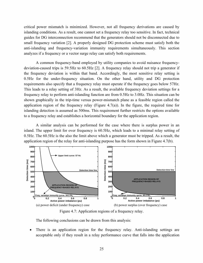
A common frequency-band employed by utility companies to avoid nuisance frequency-deviation-caused trips is 59.5Hz to 60.5Hz [2]. A frequency relay should not trip a generator if the frequency deviation is within that band. Accordingly, the most sensitive relay setting is 0.5Hz for the under-frequency situation. On the other hand, utility and DG protection requirements also specify that a frequency relay must operate if the frequency goes below 57Hz. This leads to a relay setting of 3Hz. As a result, the available frequency deviation settings for a frequency relay to perform anti-islanding function are from 0.5Hz to 3.0Hz. This situation can be shown graphically in the trip-time versus power-mismatch plane as a feasible region called the application region of the frequency relay (Figure 4.7(a)). In the figure, the required time for islanding detection is assumed as 500ms. This requirement further restricts the options available to a frequency relay and establishes a horizontal boundary for the application region.

A similar analysis can be performed for the case where there is surplus power in an island. The upper limit for over frequency is 60.5Hz, which leads to a minimal relay setting of 0.5Hz. The 60.5Hz is the also the limit above which a generator must be tripped. As a result, the application region of the relay for anti-islanding purpose has the form shown in Figure 4.7(b).

0 0.2 0.4 0.6 0.8 1 0 100 200 300 400 500 600 700 800 900

1000

Active power imbalance (pu)

Det

ectio

n tim

e (m

s)

APPLICATION REGION OF FREQUENCY - BASED RELAYS

D etection time line

Upper limit curve: 57 Hz

Freq. variation immunity curve: 59.5 Hz

0 0.2 0.4 0.6 0.8 1 0 100 200 300 400 500 600 700 800 900

1000

Active power imbalance (pu)

Det

ectio

n tim

e (m

s)

APPLICATION REGION OF FREQUENCY - BASED RELAYS

Detection time line

Freq. variation immunity curve: 60.5 Hz

(a) power deficit (under frequency) case (b) power surplus (over frequency) case

Figure 4.7: Application regions of a frequency relay.

The following conclusions can be drawn from this analysis:

• There is an application region for the frequency relay. Anti-islanding settings are acceptable only if they result in a relay performance curve that falls into the application

26

region. Operating close to the boundary of the region for the purpose of improving anti-islanding sensitivity is likely to increase the chances for nuisance generator trips.

• Because of the restriction of the application region, a non-detection zone in the range of at least 10% to 20% power mismatch always exists when a frequency relay is applied for anti-islanding protection. This region is more significant for power deficit (under frequency) case than for the power surplus (over frequency) case.

• In order to improve the anti-islanding performance, one may choice to use one setting for under-frequency case and another for the over-frequency case. Such a relay is expected to have a smaller overall non-detection zone for both power deficit and surplus case.

4.2.5 Limitation of the ROCOF Relay

The ROCOF relay is based on the rate of frequency change. The rate of frequency change is essentially in proportion to the power imbalance in the islanded system. As a result, if the power mismatch is smaller than certain value, the rate of frequency change may never exceed the ROCOF relay setting, even if the frequency has deviated from its nominal value significantly. It implies that the ROCOF relay has an inherent non-detection zone. The following analysis will clarify this subject further.

The swing equation of an islanded synchronous generator has the following form:

⎪⎪⎩

⎪⎪⎨

⎧

−=

Δ=−=−=

0

0

2

ωωδ

ωω

dtd

PPPPdtdH

SYSLM

(6)

where H is the generator inertia constant, ω0 = 2πf0 is the synchronous speed, f0 is the system nominal frequency and ΔP is the power mismatch in the island. The rate of change of frequency can be calculated as:

HPP

Hf

dtd

dtdf Δ

=Δ== 3022

1 0ωπ

(7)

The above equation shows that the rate of change of frequency is proportional to the power imbalance. If we omit the averaging process needed to determine df/dt and the associated time delays, the relay activation criterion becomes:

β>=Δ

dtdf

HP30 or 30/β>

ΔHP

(8)

27

where β is the relay setting. The above equation defines the theoretical (i.e. the minimal) non-detection zone of the ROCOF relay. For example, if β=1.5Hz/s, the minimal normalized power imbalance required to trigger the relay is 0.05 per-unit, which corresponds to the vertical line shown in Figure 4.6(b).

4.3 Performance Curves of the Voltage Relay

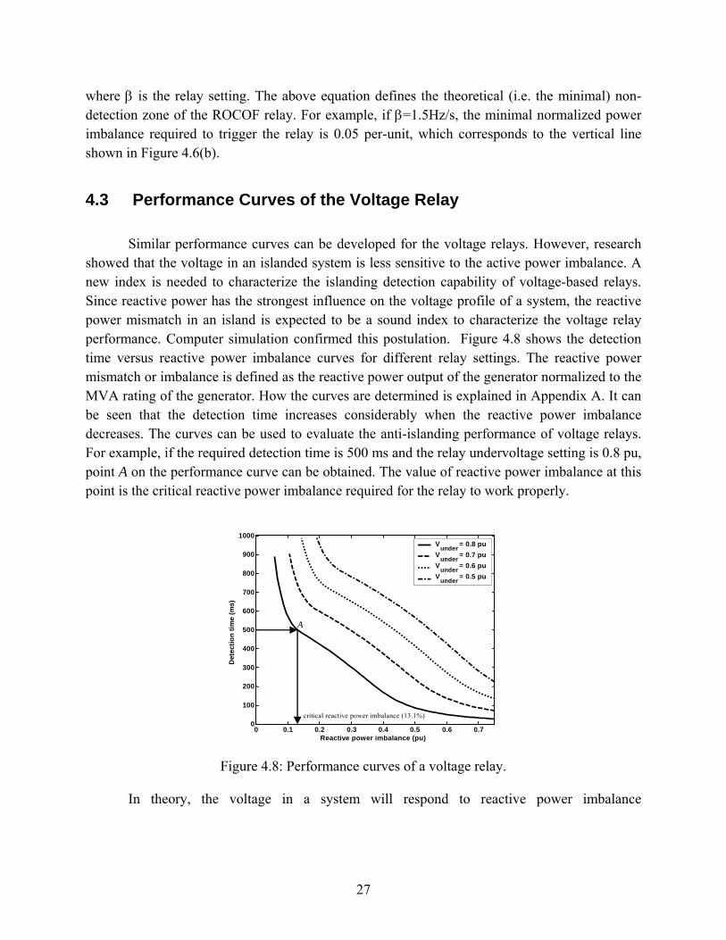
Similar performance curves can be developed for the voltage relays. However, research showed that the voltage in an islanded system is less sensitive to the active power imbalance. A new index is needed to characterize the islanding detection capability of voltage-based relays. Since reactive power has the strongest influence on the voltage profile of a system, the reactive power mismatch in an island is expected to be a sound index to characterize the voltage relay performance. Computer simulation confirmed this postulation. Figure 4.8 shows the detection time versus reactive power imbalance curves for different relay settings. The reactive power mismatch or imbalance is defined as the reactive power output of the generator normalized to the MVA rating of the generator. How the curves are determined is explained in Appendix A. It can be seen that the detection time increases considerably when the reactive power imbalance decreases. The curves can be used to evaluate the anti-islanding performance of voltage relays. For example, if the required detection time is 500 ms and the relay undervoltage setting is 0.8 pu, point A on the performance curve can be obtained. The value of reactive power imbalance at this point is the critical reactive power imbalance required for the relay to work properly.

0 0.1 0.2 0.3 0.4 0.5 0.6 0.70

100

200

300

400

500

600

700

800

900

1000

Det

ectio

n tim

e (m

s)

Reactive power imbalance (pu)

Vunder = 0.8 puVunder = 0.7 puVunder = 0.6 puVunder = 0.5 pu

critical reactive power imbalance (13.1%)

A

Figure 4.8: Performance curves of a voltage relay.

In theory, the voltage in a system will respond to reactive power imbalance

28

instantaneously. Due to the time constants of the generator electric circuit1, the voltage response does take time. So the time taken to exhibit detectable voltage change is related to the DG time constants.

4.3.1 Key Factors Affecting the Relay Performance

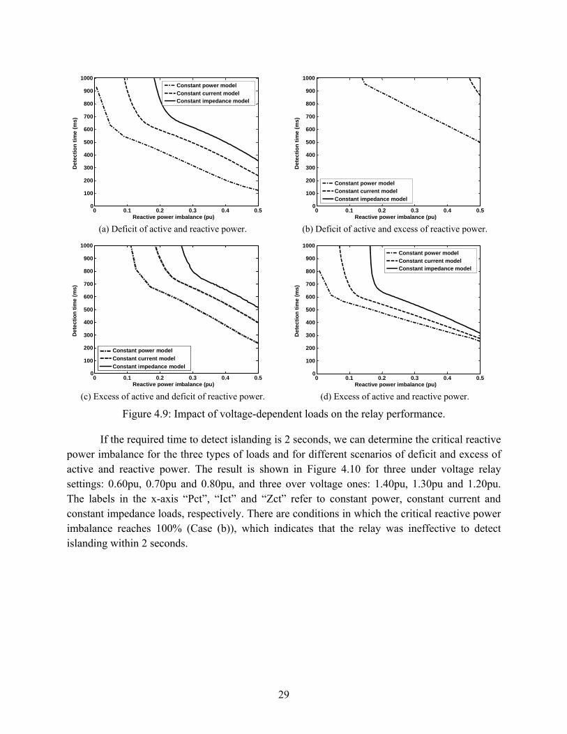
Although simple in concept, the voltage relay has complex responses to some of the system conditions. One of the key conditions is associated with load composition in the system. As expected, the presence of voltage-dependent loads in an island will affect the relay performance. It was found that the effect also depends on nature of active and reactive power mismatches. Figure 4.9 presents anti-islanding performance of a voltage relay under four different power mismatch scenarios for an under-voltage setting of 0.7pu and over-voltage setting of 1.3pu (case (a) to (d)). The figure reveals that the smallest critical reactive power im-balances are related to the constant power load cases, and the largest critical reactive power imbalances are related to the constant impedance load cases. This is understandable since the reactive power demand in an island can drop significantly if the load is constant impedance type and if the voltage drops. This will reduce the power mismatch of the island, leading to longer time to detect the voltage drop. When constant power loads are present, the nodal voltages decrease faster than that case of constant impedance loads so it is easier to detect a voltage change. For case (b), deficit of active and excess of reactive power, the constant impedance load causes so little voltage change and the voltage relay cannot detect the islanding situation. The conclusion is that if load composition is unknown, the relay performance and non-detection zone may have to be assessed using the conservative constant impedance load models.

1 The equivalent circuit of a generator can be modeled using Park's equation. A generator responds to disturbances through subtransient reactance and time constant initially, which is then followed by transient reactance and time constants. Islanding is a form of disturbance and it takes time for an islanded DG to reach a new voltage steady-state so it takes time to detect sufficient voltage deviation.

29

0 0.1 0.2 0.3 0.4 0.50

100 200 300 400 500 600 700 800 900

1000

Reactive power imbalance (pu)

Det

ectio

n tim

e (m

s)

Constant power modelConstant current modelConstant impedance model

(a) Deficit of active and reactive power.

0 0.1 0.2 0.3 0.4 0.50

100

200

300

400

500

600

700

800

900

1000

Reactive power imbalance (pu)

Det

ectio

n tim

e (m

s)

Constant power modelConstant current modelConstant impedance model

(b) Deficit of active and excess of reactive power.

0 0.1 0.2 0.3 0.4 0.50

100 200 300 400 500 600 700 800 900

1000

Reactive power imbalance (pu)

Det

ectio

n tim

e (m

s)

Constant power model Constant current model Constant impedance model

(c) Excess of active and deficit of reactive power.

0 0.1 0.2 0.3 0.4 0.50

100

200

300

400

500

600

700

800

900

1000

Reactive power imbalance (pu)

Det

ectio

n tim

e (m

s)

Constant power modelConstant current modelConstant impedance model

(d) Excess of active and reactive power.

Figure 4.9: Impact of voltage-dependent loads on the relay performance.

If the required time to detect islanding is 2 seconds, we can determine the critical reactive power imbalance for the three types of loads and for different scenarios of deficit and excess of active and reactive power. The result is shown in Figure 4.10 for three under voltage relay settings: 0.60pu, 0.70pu and 0.80pu, and three over voltage ones: 1.40pu, 1.30pu and 1.20pu. The labels in the x-axis “Pct”, “Ict” and “Zct” refer to constant power, constant current and constant impedance loads, respectively. There are conditions in which the critical reactive power imbalance reaches 100% (Case (b)), which indicates that the relay was ineffective to detect islanding within 2 seconds.

30

0,1

1

10

100

Pct Ict Zct Pct Ict Zct Pct Ict Zct 0.60/1.40 0.70/1.30 0.80/1.20

Voltage relay settings (pu)

Crit

ical

reac

tive

pow

er im

bala

nce

(%) Case (a)

Case (b) Case (c) Case (d)

Figure 4.10: Critical reactive power imbalances for different type of voltage-dependent loads.

Other factors that could potentially affect the relay performance have been investigated. The following summarizes the main conclusions:

• Generator excitation control mode: As discussed earlier, a DG has two excitation control modes, one is to maintain constant terminal voltage (voltage control mode) and the other is to maintain constant power factor (power factor or reactive power control mode). It was found that the voltage relay is ineffective to detect islanding conditions if a DG is in voltage control mode. This is easy to understand since the goal of the mode is to maintain a constant generator terminal voltage. The relay performance curves shown in this Section are all related to the power factor control mode.

• Load power factor: Impact of load power factor on relay performance depending on the amount of reactive power output of the DG before islanding occurs. Research results show that the critical power mismatch can increase by about 20% when the load power factor changes from 0.7 to 0.9. In reality, however, the load power factors are around 0.95 and they do not vary a lot. The impact of power factor is therefore not significant.

• The line length and line X/R ratio have no significant impact on the relay performance.

• The active power mismatch has an impact on relay performance. This subject will be discussed in the next Chapter from the perspective of 2D non-detection zones.

4.3.2 Limitations of Voltage Relay

Similar to the frequency relay, the voltage relay has limitations due to the conflicting requirements of anti-islanding protection and immunity to minor voltage deviations. As a result, one cannot set a voltage relay too sensitive for anti-islanding protection since it may result in

31

excessive nuisance relay operations. Table 4.2 shows current industry recommendations on DG voltage relay settings against abnormal voltage variation [2]. It can be seen from this table, a voltage relay is not expected to operate when the voltage resides between 0.88 to 1.10 per-unit.

Table 4.2: Protection requirements against abnormal voltage variations.

Voltage (pu) Clearing time (s)

< 0.50 0.16 0.50 – 0.88 2.00 1.10 – 1.20 1.00

≥ 1.20 0.16

Accordingly, the most sensitive relay setting is 0.88pu for the under-voltage situation and 1.10pu for the over-voltage situation. This situation can be shown graphically in the detection-time versus power-mismatch plane in the form an application region of the voltage relay (Figure 4.11). In the figure, the required time for islanding detection is assumed as 500 ms. This requirement further restricts the options available to a voltage relay and establishes a horizontal boundary for the application region. From the figures, we can conclude that the non-detection zone for a voltage relay is at least 10%.

0 0.1 0.2 0.3 0.4 0.50

100

200

300

400

500

600

700

800

900

1000

Reactive power imbalance (pu)

Det

ectio

n tim

e (m

s)

Application Region

0 0.1 0.2 0.3 0.4 0.5

0

100

200

300

400

500

600

700

800

900

1000

Reactive power imbalance (pu)

Det

ectio

n tim

e (m

s)

Application Region

(a) reactive power deficit (under voltage) case (b) reactive power surplus (over voltage) case

Figure 4.11: Application region of a voltage relay.

32

CHAPTER 5: NON-DETECTION ZONES OF COMBINED FREQUENCY AND VOLTAGE RELAYS

The relay operating characteristics presented in the last Chapter suggest that each type of relay has a non-detection zone. The non-detection zone of frequency-based relays is strongly associated with the active power imbalance in an island while that of the voltage relay can be affected by both active and reactive power imbalances. For a given detection time requirement, there is a critical power mismatch. If the power imbalance in an islanding is smaller than the critical mismatch, the relay is unlikely to detect the islanding situation within the specified time. For common DG installations, both frequency-based and voltage-based relays are used. It becomes possible that an islanding condition can still be detected even if one of the power imbalances is smaller than its corresponding critical power mismatch. In other words, a combined use of frequency and voltage relays will enhance the anti-islanding capability of a DG installation. The goal of this chapter is to investigate the anti-islanding characteristics for combined frequency and voltage relays. A two-dimensional non-detection zone (NDZ) is introduced to represent the characteristics.

5.1 The Concept of 2D Non-Detection Zone in PQ Plane

There are two aspects of power imbalance in an island. One is the active power imbalance and the other is the reactive power imbalance. Any particular power imbalance situation in an island can therefore be presented as a point in the ΔP and ΔQ plane as shown in Figure 5.1, where Δ denotes power imbalance (a positive value denotes surplus power). There is also a detection time associated with the operating point, which can be illustrated using a 3rd axis shown in Figure 5.1(a). If one specifies a required detection time, there will be cases whose ΔP and ΔQ values are not sufficient to result in a timely detection of the islanding situation. These cases or points in the PQ plane define a non-detection zone. Figure 5.1(b) is an illustrative plot of such a non-detection zone.

ΔP

ΔQ

Detection Time

ΔP

ΔQ

Non-detection zone for a requireddetection time

(a) Detection time for a given power imbalance case (b) Non-detection zone in PQ plane

Figure 5.1: Power imbalance situation in PQ plane and the associated non-detection zone.

33

In the following sections, the NDZs of frequency and voltage relays are determined individually first. They are then combined to show the NDZs when both relays are used for anti-islanding detection. Due to the complexity of the problem, computer simulation on a sample distribution system is the main tool to determine the non-detection zones.

5.2 Non-detection Zone of the Frequency Relay

Figure 5.2 shows the non-detection zones (NDZ) of a standard frequency relay for the case where the generator exciter is on voltage control mode, the load is constant power type and the detection time is 500ms. The active and reactive power imbalances were varied from –1 to 1 pu by changing load-generation scenario of the electrical system. The power basis used is the synchronous machine rated power. There are two zones each corresponding to a different relay setting. It can be seen that the left and right boundaries of the NDZ are almost vertical. This implies that the relay performance is indifferent to reactive power imbalance, which is supported by the results of Chapter 4. There are top and bottom boundaries for the NDZ as well. The boundaries are caused by the steady-state voltage limits at the DG terminal, which are 0.95pu and 1.05pu respectively. In other words, a feasible operating point does not exist for the regions above or below the horizontal boundaries. If the voltage limits were not considered, the NDZ would be a vertical bend.

-1.1 -0.9 -0.7 -0.5 -0.3 -0.1 0.1 0.3 0.5 0.7 0.9 1.1 -0.7

-0.5

-0.3

-0.1

0.1

0.3

Active power imbalance (pu)

Rea

ctiv

e po

wer

imba

lanc

e (p

u)

Setting 1: 57.5 Hz / 62.5 HzSetting 2: 58.5 Hz / 61.5 HzSteady-state Voltage LimitsSimulated ΔP Intervals

Figure 5.2: Non-detection zone of a frequency relay

If the load becomes voltage dependent, the NDZ will be affected by reactive power mismatch. Figure 5.3(a) compares the NDZs for the constant power, constant current and constant impedance loads. It can be seen that when a load becomes more voltage dependent, the NDZ becomes more skewed and the impact of reactive power mismatch becomes larger. Figure 5.3(b) shows the impact of DG excitation control modes. The NDZs correspond to constant

34

impedance load and a relay setting of 57.5/62.5Hz. It can be seen that the power factor (or Q) control mode gives slightly larger NDZ. This behavior is due to the voltage variation after the islanding occurrence: under the Q control mode, the voltage can increase or decrease monotonically. On the other hand, the voltage control mode tries to maintain the terminal voltage. The resulting voltage variation is not as significant as the case of Q control mode.

- 1.1 - 0.9 - 0.7 - 0.5 - 0.3 - 0.1 0.1 0.3 0.5 0.7 0.9 1.1 - 0.7

- 0.5

- 0.3

- 0.1

0.1

0.3

Active power imbalance (pu)

Rea

ctiv

e po

wer

imba

lanc

e (p

u)

Con stant Power Constant Current Constant Impedance Steady - state Voltage Limits Simulated Δ P Intervals

-1.1 -0.9 -0.7 -0.5 -0.3 -0.1 0.1 0.3 0.5 0.7 0.9 1.1 -0.7

-0.5

-0.3

-0.1

0.1

0.3

Active power imbalance ( )

R

eact

ive

pow

er im

bala

nce

V Control Q Control Steady-state Voltage Limits Simulated Δ P Intervals

(a) Impact of island load characteristics.

(voltage control mode) (b) Impact of DG excitation control mode.

(constant impedance load) Figure 5.3: Variation of frequency relay's non-detection zone.

5.3 Non-detection Zone of the Voltage Relay

Figure 5.4 shows the non-detection zone of a voltage relay for the case of constant power load, reactive power control mode and detection time of 500ms. It has been shown in Chapter 4 that a voltage relay is ineffective when the DG is in voltage control mode so Figure 5.4 shows the NDZ associated with the reactive power control mode. Two groups of settings are compared: 0.8 pu (under voltage) and 1.2 pu (over voltage) versus 0.7 pu/1.3 pu. It can be seen that the NDZ resembles a horizontal bend. This indicates that the relay performance is strongly affected by reactive power imbalance. The impact of active power imbalance can also been seen since the NDZ is skew downward at the right. The two vertical boundaries correspond to 100% active power mismatch, which is the boundary of our study concern. The steady-state voltage limits also play a (small) role in shaping the NDZ - the top left boundary is caused by the voltage limits. It can be seen that the non-detection zone of the voltage relay is much larger than that of the frequency relay. Even in case of large active power imbalances, the voltage relay does not operate if there is not a proper amount of reactive power imbalance.

35

-1.1 -0.9 -0.7 -0.5 -0.3 -0.1 0.1 0.3 0.5 0.7 0.9 1.1-0.7

-0.5

-0.3

-0.1

0.1

0.3

Active power imbalance (pu)

Rea

ctiv

e po

wer

imba

lanc

e (p

u)

Setting 1: 0.80 pu/1.20 puSetting 2: 0.70 pu/1.30 puSteady-state Voltage LimitsSimulated ΔP Intervals

Figure 5.4: Non-detection zone of a voltage relay.

The impact of voltage dependent load on the NDZ can be seen from Figure 5.5(a). The constant impedance load also leads to the largest NDZ for the voltage relay. Figure 5.5(b) shows the effect of excitation control. As expected, the voltage control mode leads to a larger NDZ.

- 1.1 - 0.9 - 0.7 - 0.5 - 0.3 - 0.1 0.1 0.3 0.5 0.7 0.9 1.1 - 0.7

- 0.5

- 0.3

- 0.1

0.1

0.3

Active power imbalance (pu)

Rea

ctiv

e po

wer

imba

lanc

e (p

u)

Con stant Power Constant Current Constant Impedance Steady - state Voltage Limits Simulated Δ P Intervals

-1.1 -0.9 -0.7 -0.5 -0.3 -0.1 0.1 0.3 0.5 0.7 0.9 1.1 -0.7

-0.5

-0.3

-0.1

0.1

0.3

Active power imbalance (pu)

Rea

ctiv

e po

wer

imba

lanc

e (p

u)

V Control Q Control Steady-state Voltage Limits Simulated ΔP Intervals

(a) Impact of island load characteristics. (reactive power control mode)

(b) Impact of DG excitation control mode. (constant impedance load)

Figure 5.5: Variation of voltage relay's non-detection zone.

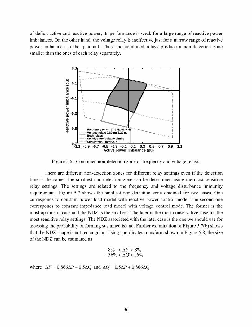
5.4 Non-Detection Zone of Combined Frequency and Voltage Relays

The non-detection zone of combined frequency and voltage relays is the union of the individual non-detection zones associated with each type of relays. A sample result of the combined NDZ for a frequency relay setting of 57.5/62.5 Hz and voltage relay setting of 0.8/1.2 pu is shown in Figure 5.6. The case corresponds to constant impedance load, reactive power control mode and 500ms detection time. It can be seen that for the most of the operating scenarios, the frequency relay has better performance than the voltage relay, but in the quadrant

36

of deficit active and reactive power, its performance is weak for a large range of reactive power imbalances. On the other hand, the voltage relay is ineffective just for a narrow range of reactive power imbalance in the quadrant. Thus, the combined relays produce a non-detection zone smaller than the ones of each relay separately.

- 1.1 - 0.9 - 0.7 -0.5 -0.3 -0.1 0.1 0.3 0.5 0.7 0.9 1.1 - 0.7

- 0.5

- 0.3

- 0.1

0.1

0.3

Active power imbalance (pu)

Rea

ctiv

e po

wer

imba

lanc

e (p

u)

Frequ ency relay: 57.5 Hz/62.5 HzVoltage relay: 0.80 pu/1.20 puBoth relaysSteady - state Voltage LimitsSimulated ΔP Intervals

Figure 5.6: Combined non-detection zone of frequency and voltage relays.

There are different non-detection zones for different relay settings even if the detection time is the same. The smallest non-detection zone can be determined using the most sensitive relay settings. The settings are related to the frequency and voltage disturbance immunity requirements. Figure 5.7 shows the smallest non-detection zone obtained for two cases. One corresponds to constant power load model with reactive power control mode. The second one corresponds to constant impedance load model with voltage control mode. The former is the most optimistic case and the NDZ is the smallest. The later is the most conservative case for the most sensitive relay settings. The NDZ associated with the later case is the one we should use for assessing the probability of forming sustained island. Further examination of Figure 5.7(b) shows that the NDZ shape is not rectangular. Using coordinates transform shown in Figure 5.8, the size of the NDZ can be estimated as

%16'%36%8'%8

<Δ<−<Δ<−

QP

where QPP Δ−Δ=Δ 5.0866.0' and QPQ Δ+Δ=Δ 866.05.0'

37

- 1.1 - 0.9 - 0.7 - 0.5 - 0.3 - 0.1 0.1 0.3 0.5 0.7 0.9 1.1 - 0.7

- 0.5

- 0.3

- 0.1

0.1

0.3

Active power imbalance (pu)

Rea

ctiv

e po

wer

imba

lanc

e (p

u)

Constant P - Q control Steady - state Voltage Limits Simulated Δ P Intervals

-1.1 -0.9 -0.7 -0.5 -0.3 -0.1 0.1 0.3 0.5 0.7 0.9 1.1 -0.7

-0.5

-0.3

-0.1

0.1

0.3

Active power imbalance (pu)

Rea

ctiv

e po

wer

imba

lanc

e (p

u)

Constant Z - V control Steady-state Voltage Limits Simulated Δ P Intervals

(a) Smallest non-detection zone (reactive power control mode, constant power load, detection time = 500 ms)

(b) Conservative non-detection zone for the most sensitive relay settings (constant voltage control mode,

constant impedance load, detection time = 500 ms)

Figure 5.7: NDZ associated with the most sensitive relay settings.

- 1.1 - 0.9 - 0.7 - 0.5 - 0.3 - 0.1 0.1 0.3 0.5 0.7 0.9 1.1 - 0.7

- 0.5

- 0.3

- 0.1

0.1

0.3

Active power imbalance (pu)

Rea

ctiv

e po

wer

imba

lanc

e (p

u)

Constant Z - V control Steady - state Voltage Limits Simulated Δ P Intervals

ΔP’

ΔQ’

Estimated NDZ

Figure 5.8: Recommended NDZ for the most sensitive relay settings.

38

CHAPTER 6: THE RISK OF ISLAND FORMATION

The risk of islanding formation is essentially the probability of a DG-containing distribution system entering the non-detection zones created by the anti-islanding devices. Starting from this Chapter, we will analyze the risks of islanding formation and present a practical method for risk assessment. The main objective of this research work is to assist Canadian utility companies to evaluate the anti-islanding protection needs of a synchronous DG installation proposal properly, which will, in turn, reduce the interconnection barrier of environmental friendly distributed generators.

6.1 The Concept of Islanding Risk

The frequency and voltage-based relays are the first choice for anti-islanding protection of distributed generators. Since all of these relays have non-detection zones, it is necessary to understand the actual probability that an island will occur and what risks this unintentional island will present to human safety and the electrical network. This allows the benefits of further risk reduction from more reliable anti-islanding schemes to be balanced against the costs imposed by these schemes. If a simple and low cost anti-islanding scheme such as that offered by combined frequency and voltage relays reduces the risk to a level below other electrical safety risks that are currently considered acceptable, it is debatable whether a scheme with better detection performance, but higher costs (in financial or performance terms), is necessary. This is particularly true when the DG reduces other hazards, such as air pollution.

The frequency relay is used here as an example to illustrate the risk of non-detection or unintentional formation of an island. As shown in the previous chapters, the frequency-based anti-islanding scheme cannot detect the formation of an island within required time if the active power mismatch in the island is small. According to Figure 5.2, the power mismatch threshold can be as high as ±30% depending on the relay setting and other factors. There are two factors that can significantly affect the actual power mismatch levels in an island. The first factor is the daily variation of feeder loads. Depending on their operating characteristics, feeder loads could have ±20% variation around its daily average. The second factor is that different islands could be formed with a DG. Each island will have different load levels (Figure 6.1). Both factors will work together to create more situations where small power mismatch levels could be encountered, leading to increased risk of non-detection. This situation is illustrated in Figure 6.2.

39

DG

SubstationRecloser 1 Recloser 2

Fault 2Fault 1

Island 1Island 2

Figure 6.1: Example scenarios of island formation.

hour

load

DG generation level

Island condition 1 Island formation 1

Notokay

Notokay

Notokay

Notokay

Notokay

Notokay

Load

Time of a day

Non-detectionzone

}Island formation 2

hour

load

DG generation level

Island condition 1 Island formation 1

Notokay

Notokay

Notokay

Notokay

Notokay

Notokay

Load

Time of a day

Non-detectionzone

}Island formation 2

Figure 6.2: The impact of non-detection zone for islanding detection.

The figure shows the variation of load level during a 24-hour period. Two load variation curves are shown. Each curve corresponds to a different island formation scenario. The power output of the DG is assumed as constant during the 24-hour period. So it is a horizontal line. The intersections of the DG curve and the load variation curves represent the cases where there is a zero mismatch between load and generation. The non-detection zone is shown as a shaded band.

40

Any load values that fall into the band will result in poor detection of islanding conditions (marked as 'not okay' in the figure). It can be seen that there is a number of operating periods during which poor or no detection of islanding conditions can occur. If more islanding scenarios are added (i.e. if there are more load variation curves), such periods will increase further. This analysis shows that the risk associated with non-detection zone is real and can be significant.

The above analysis just considers the factor that an operating condition enters into the relay’s non-detection zone. We can denote the probability of it happening as PND, where ND stands for non-detection. It must be noted that two more factors need to be considered if a DG does create a hazard due to islanding. The first factor is the probability of faults or operations that result in an islanded network configuration, which can be denoted as Pcause. The second factor is the probability of a sustained island manifesting into a safety consequence such as electric shock or into a power quality consequence involving equipment damage. This probability is labelled as Pconsequence. The probability of hazard resulting from unintentional islanding can thus be estimated as

econsequencNDcausehazard PPPP ××=

Characteristics of the above three factors are discussed below:

• Pcause: A utility has little control on this factor or, more precisely, it is not practical to expect a utility to reduce Pcause for the purpose of reducing Phazard. Furthermore, the majority of utility protection schemes are implemented independent of the probability of fault occurrence. So an anti-islanding protection is needed no matter how small Pcause is.

• PND: This is the main factor of concern to utility companies. It is the basis of specifying anti-islanding protection requirements for DG interconnection proposals. Utility companies have a good control over this factor to reduce the hazard of unintentional islanding.

• Pconsequence: Utility companies have some control over this factor, especially the factor involving human hazard. To make it work, the companies have to change their practice and the costs (such as training) could be significant. It is not realistic to expect a utility company to accommodate a particular DG installation in this way. However, a utility-wide practice change may be possible. From this perspective, Pconsequence is unlikely to affect the evaluation of a particular DG interconnection request. Another factor worthy consideration is that a utility company may not accept a sustained island at all no matter how small Pconsequence is.

The goal of this project is to help utility companies to evaluate the applicability of low-cost anti-islanding protection schemes. The main focus of this research is, therefore, the factor of PND. This is the only factor that is related to the anti-islanding schemes and is DG case specific. In the following sections, we will propose a method to calculate PND and analyze its characteristics.

41

There is a value to calculate Phazard, which has been done for the residential photovoltaic distributed generators (see the review in the next section) [5,6]. The main goal of such research is to show that unintentional islanding should not be a significant concern to utility companies and other stakeholders. This research deals with synchronous DGs connected to the medium voltage distribution systems. Unlike the residential photovoltaic systems, the risk of hazard for synchronous DG is case specific and it is not possible to draw general conclusions. As a result, quantifying the general risk of islanding-caused hazard for synchronous DGs may not be achievable. This subject will be discussed further in the next section.

6.2 Survey of Islanding Risk Research

Power industry has quite diverse viewpoints on the non-intentional islanding of distributed generators. While some treat the islanding as a rare event, others are strongly concerned with its occurrence and the associated effects to the distribution systems. These different opinions arise due to the types of distributed generation technology, the penetration level of DGs and the distribution system characteristics. This section presents a literature survey on the risk evaluation of DG-caused non-intentional islanding. It was found that essentially all of the work is related to the PV-type distributed generators. Risk assessment research for other types of DG technologies was not found in the literature.

One of the earliest studies on this subject was presented in [13]. In this paper, the authors proposed an optimum islanding prevention method for small-scale PV systems. The method was based on simulation analysis concerning the occurrence probability of non-intentional islanding, and its effectiveness was evaluated using the Rokko Islanding 200 kW PV facility in Japan. Only islanding prevention methods based on local active and passive measures were adopted. Among the passive methods, abnormal voltage and frequency, phase monitoring measure, harmonic monitoring measure and frequency change rate monitoring were considered. For active methods, frequency bias and output power variation were employed. The basic methodology developed by the authors involves the calculation of the number of islanding events per year for different PV penetration rates. Penetration ratio was defined in the paper as the ratio of overall PV capacity to supply system capacity. For each level of PV power output and load combination, an electromagnetic simulation was performed to verify if the islanding was detected. Main conclusions of the paper are: 1) for connection densities below 30%, islanding is virtually impossible if only voltage and frequency are monitored for islanding detection; 2) when the PV penetration ratio is higher than 40%, combination of two or more anti-islanding schemes are necessary to reduce the probability of islanding; 3) for the worst-case connection density of 80%, the probability of non-intentional islanding reached approximately 6.7% when voltage and frequency based islanding scheme are used. If additional islanding detection methods are implemented, the probability can be reduced considerably; 4) the PV penetration level affects the probability of islanding significantly. It can be seen that this investigation concentrates on the probability of generation-load mismatch, which is PND. The conclusions were obtained for a

42

specific test system, but the methodology can be easily applied to other distribution networks and DG schemes.

Through intensive analyses, the International Energy Agency (IEA) Task V Working Group published two reports on the probability of islanding [5] and the associated risk of human hazard [6] for low voltage distribution networks with a high penetration level of grid connected PV-systems. The conclusions, as will be presented later, are different from the ones presented in [13], although the three works deal with the same subject.

The first report [5] essentially investigates the probability of load-generation balance, which is roughly equal to PND. The study case is a representative residential area located in the city of Arnhem of the Netherlands. The loads and the PV-systems were monitored every second for two years and stored in a computer for off-line analysis. Such measurement is important since there is a correlation between load demand of the network and the power produced by the PV-systems. The main methodology of the work is to calculate the frequency and duration of the scenarios, based on the measured data, that satisfy the following condition, which is called the balanced condition by the report:

Δ<− || generationload PP

where Δ is the margin of tolerance. It is essentially the width of the non-detection zone. A non-detection zone of 2% to 20% was adopted for sensitivity analysis in the report. The reactive power balance is also considered. The ratio of the time when the system is in the balanced condition to the total time of the study period is defined as probability of islanding. The report reveals that balanced conditions occur very rarely for low, medium and high penetration levels of PV-systems. The report further concludes that the probability of power network disconnection occurring at the same time of load-generation balance, i.e. Pcause×PND, is virtually zero. As a result, islanding is therefore not a technical barrier for the large-scale deployment of PV system in residential areas.

Based on the above results, the second IEA report [6] applied formal risk analysis techniques to estimate the islanding-caused hazard associated with the residential PV systems. The aim was to perform a first pass calculation to determine the additional level of risk that islanding could present to the safety of customers and network maintenance staff. The study considered the risk to human as a combination of the probability of the loss of mains supply with the simultaneous probability of load/generation match and the failure of the protection to detect the island on demand. The probability of the loss of mains supply was determined through actual data related to the probability of power outage in typical UK distribution systems. Information regarding the probability of load/generation match was provided by [5]. Finally, the probability of failure of the protection system was estimated by considering the inverter designed safety integrity level (SIL) and the quality of the installation. Therefore, the hazardous risk to human

43

was then calculated by multiplying the probability of balanced conditions, the probability of loss of mains and the probability of detection failure. Furthermore, another multiplying term was applied regarding safe working practice. The study found that the risk of electric shock under worst-case PV penetration scenarios is typically less than 10-9 per year. In comparison, the “benchmark” or inherent risk that already exists for network operators and customers is of the order of 10-6 per year. Thus, the additional risk presented by islanding does not materially increase the risk that already exists as long as the risk is managed properly.

In [14], the authors analysed the risk issue of the PV systems considering the frequency and voltage based inverter anti-islanding protection schemes. This work concludes that the margin values, i.e. the non-detection zones, can be considerably larger than the 5% value for the active and 2% for the reactive power adopted by the IEA studies [5] and [6]. The authors further recommended that the IEA studies be reinterpreted by considering the actual non-detection zones of the protective devices and the quality factors of loads. One of the conclusions of the report is that for networks with a high density of PV generation the probability of island formation due to non-detection zones of standard protective relays may not be negligible. In order to keep the risk of non-intentional islanding for maintenance operators and customers satisfactorily low, additional islanding prevention methods are necessary.

Using a methodology similar to the one employed in [5] but taking into account the protection devices non-detection zones as in [14], reference [15] determined the probability of inverter-based generation islanding in an actual low voltage network (PND). The analyses considered different generation penetration scenarios, protection’s frequency and voltage window and load characteristics. The methodology employed by the authors was based on the simultaneous measurements and records of loads and distributed generators active and reactive powers at a time resolution of 1 second. By correlating the recorded load and generation profiles for active and reactive power, possible islanding situations could be identified under different boundary conditions, e.g. protection settings or penetration levels. The authors concluded that the probability of balanced conditions depends on the penetration level of the distributed generation, reactive power supply, protection settings and generator control mode. Moreover, the overall conclusion is that in certain network environments, the probability for balanced load/generation conditions and thus the non-intentional creation of an island shall not be regarded as virtually impossible.

6.3 Strategy of the Proposed Work

The survey results reveal that no work has been done on the risk assessment of synchronous DG caused islanding situations. The synchronous DGs are much larger in comparison with the PV systems and they are connected to medium voltage systems. The impact caused by non-intentional islanding is therefore much more serious. This is why utility companies are more concerned with the interconnection of synchronous DGs. In comparison

44

with the PV-systems, the synchronous DGs have the following unique characteristics:

• A synchronous DG can have different types of energy sources such as small hydro or gas turbine. The PV system’s energy source is just one type and its operating pattern can be generalised. As a result, it is very difficult to draw general considerations as to the risk levels associated with synchronous DG islanding.

• The supply system to which a synchronous DG is interconnected can also be quite diverse. Examples are different feeder configurations and load characteristics. On the other hand, the PV system is mainly connected to the residential networks that have a similar characteristic, which makes a general analysis of PV islanding risk possible2. This is another factor suggesting a different approach is needed for the islanding risk analysis of the synchronous DGs.

• The third factor is the different relay characteristics when synchronous DGs are involved and the use of reclosers in the medium voltage distribution systems. As shown in Figure 6.2, the reclosers can create a lot more load-generation balance scenarios, resulting in higher probability of forming sustained islands. Again, the degree of load-generation balance is system dependent.

• Since medium voltages systems are involved, utility companies are more interesting in mitigating the risks associated with PND on a case by case basis. As discussed in Section 6.1, information on the probabilities of network disconnection (Pcause) and hazardous consequences (Pconsequence) is useful to utility companies but it rarely changes the decision of anti-islanding protection requirements of the utility companies.

With the above considerations, this project believes it is more useful to develop a tool that can be used by utility engineers to estimate the probability index PND for a given DG interconnection scenario. This project, therefore, follows the strategy of [5] and [14], both of which calculate the probability of load-generation balance (PND). The main difference is that this work focuses on developing a method of risk assessment while case studies are used as examples. As discussed earlier, it is impossible to derive general conclusions that are applicable to different synchronous DG cases. A tool is of more much value than probability numbers derived from a specific case study.

The subject of computing Phazard for sample synchronous DG installations is of some value. This topic could be investigated through future research projects. It is important to note that the IEA reports used two terms, probability of islanding and risk hazard to human, to describe the various aspects of the islanding issue. In this report, the term “risk” refers to the 2 Photovoltaic farms and buildings can be major DG sources. No general conclusions can be drawn as to the islanding risks of such systems either. Note that the published research work deals with the residential PV systems only.

45

probability of failing to detect an islanded situation3, PND. It is called the risk of islanding in this report for simplicity.

3 In this study, the probability of relay malfunction is not considered.

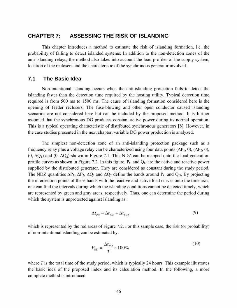
46

CHAPTER 7: ASSESSING THE RISK OF ISLANDING

This chapter introduces a method to estimate the risk of islanding formation, i.e. the probability of failing to detect islanded systems. In addition to the non-detection zones of the anti-islanding relays, the method also takes into account the load profiles of the supply system, location of the reclosers and the characteristic of the synchronous generator involved.

7.1 The Basic Idea

Non-intentional islanding occurs when the anti-islanding protection fails to detect the islanding faster than the detection time required by the hosting utility. Typical detection time required is from 500 ms to 1500 ms. The cause of islanding formation considered here is the opening of feeder reclosers. The fuse-blowing and other open conductor caused islanding scenarios are not considered here but can be included by the proposed method. It is further assumed that the synchronous DG produces constant active power during its normal operation. This is a typical operating characteristic of distributed synchronous generators [8]. However, in the case studies presented in the next chapter, variable DG power production is analyzed.

The simplest non-detection zone of an anti-islanding protection package such as a frequency relay plus a voltage relay can be characterized using four data points (ΔP1, 0), (ΔP2, 0), (0, ΔQ1) and (0, ΔQ2) shown in Figure 7.1. This NDZ can be mapped onto the load-generation profile curves as shown in Figure 7.2. In this figure, PG and QG are the active and reactive power supplied by the distributed generator. They are considered as constant during the study period. The NDZ quantities ΔP1, ΔP2, ΔQ1 and ΔQ2 define the bands around PG and QG. By projecting the intersection points of these bands with the reactive and active load curves onto the time axis, one can find the intervals during which the islanding conditions cannot be detected timely, which are represented by green and gray areas, respectively. Thus, one can determine the period during which the system is unprotected against islanding as:

21 PQPQPQ ttt Δ+Δ=Δ (9)

which is represented by the red areas of Figure 7.2. For this sample case, the risk (or probability) of non-intentional islanding can be estimated by:

%100×Δ

=Tt

P PQND

(10)

where T is the total time of the study period, which is typically 24 hours. This example illustrates the basic idea of the proposed index and its calculation method. In the following, a more complete method is introduced.

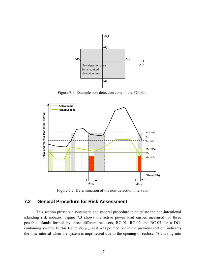
47

Δ P

Δ Q

Non-detection zone for a required detection time

ΔP1 ΔP2

ΔQ1

ΔQ2

Figure 7.1: Example non-detection zone in the PQ plan.

Act

ive

and

reac

tive

load

(MW

, MV

Ar)

Time (24h)

ΔtPQ1 ΔtPQ2

PG

PG + |ΔP2|

PG - ΔP1

QG

QG + |ΔQ2|

QG - ΔQ1

Active load Reactive load

Figure 7.2: Determination of the non-detection intervals.

7.2 General Procedure for Risk Assessment

This section presents a systematic and general procedure to calculate the non-intentional islanding risk indexes. Figure 7.3 shows the active power load curves measured for three possible islands formed by three different reclosers, RC-01, RC-02 and RC-03 for a DG-containing system. In this figure ΔtP-RCi, as it was pointed out in the previous section, indicates the time interval when the system is unprotected due to the opening of recloser “i”, taking into

48

consideration the active power balance only. Thus, generalizing, the total time when the system is unprotected due to active power balance is given by:

ΔtP =ΔtP-RC1 ∪ ΔtP-RC2 …∪ ΔtP-RCn (11)

where ∪ is the union operator and n is the number of reclosers. Using the same approach, the total time when the system is unprotected due to reactive power balance can be determined as (Figure 7.4):

ΔtQ =ΔtQ-RC1 ∪ ΔtQ-RC2 …∪ ΔtQ-RCn (12)

0 200 400 600 800 1000 1200 14000

Time duration (min)

Act

ive

load

(MW

)

Active power load curve – RC-01

PG

PG + |ΔP2|

PG - ΔP1

ΔtP-RC1

ΔtP-RC2ΔtP-G =ΔtP-RC1 ∪ ΔtP-RC2 ∪ ΔtP-RC3

ΔtP-RC3

Active power load curve – RC-02 Active power load curve – RC-03

Figure 7.3: Total unprotected time ΔtP due to the active power balance.

49

0 200 400 600 800 1000 1200 14000

Time duration (min)

Rea

ctiv

e lo

ad (M

VAr)

QG

QG + |ΔQ2|

QG - ΔQ1

ΔtQ-RC3ΔtQ-RC2ΔtQ-RC1

ΔtQ-G =ΔtQ-RC1 ∪ ΔtQ-RC2 ∪ ΔtQ-RC3

Reactive power load curve – RC-01 Reactive power load curve – RC-02 Reactive power load curve – RC-03

Figure 7.4: Total unprotected time ΔtQ due to the reactive power balance.

The failure to detect island formation is caused by the simultaneous load-generation balance of active and reactive power for all possible island formations. The global time interval ΔtG, illustrated by the blue areas in Figure 7.5, during which the system is unprotected can thus be determined by:

ΔtG =ΔtP-G ∩ ΔtQ-G (13) where ∩ denotes the intersection operator. Accordingly, the risk index representing the probability of forming non-intentional island can be calculated as follows:

%100×Δ

=TtP G

ND (14)

50

0 200 400 600 800 1000 1200 1400 0

Time duration (min)

Rea

ctiv

e lo

ad (M

VAr)

ΔtQ-G

0 200 400 600 800 1000 1200 1400 0

Time duration (min)

Act

ive

load

(MW

) ΔtP-G

ΔtG = ΔtP-G ∩ ΔtQ-G

Figure 7.5: Global unprotected time interval ΔtG.

Note that the active power load curves are normally known. On the other hand, the reactive power load curves may not be available. Since most distribution systems have reactive power compensation devices that correct the power factor to 0.94 or higher, one solution, which is adopted in this report, is to assume that the reactive power load curve is similar to the active power curve. For example, the reactive power load curve can be estimated by assuming a constant 0.94 inductive power factor. Therefore, in this case, the reactive power load curve is proportional to the active power load curve. Thus, the active and reactive load duration curves can be used to graphically understand the proposed approach as an alternative to the daily active and reactive power load curves. Figures 7.3, 7.4 and 7.5 can be modified to include the load duration curve representation as shown in Figures 7.6, 7.7 and 7.8. Equations 11 through 14 are equally employed to calculate ΔtP, ΔtQ and the global time interval ΔtG.

51

0 200 400 600 800 1000 1200 14000

Time duration (min)

Act

ive

load

(MW

) PG

PG + |ΔP2|

PG - ΔP1

ΔtP-RC3 ΔtP-RC2

ΔtP-RC1

ΔtP-G =ΔtP-RC1 ∪ ΔtP-RC2 ∪ ΔtP-RC3

Active power load duration curve – RC-01 Active power load duration curve – RC-02 Active power load duration curve – RC-03

Figure 7.6: Total unprotected time ΔtP due to the active power balance, considering load duration curves.

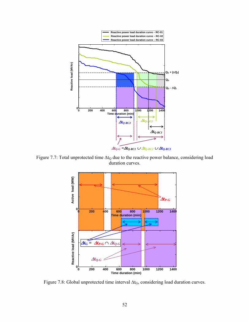
52

0 200 400 600 800 1000 1200 14000

Time duration (min)

Rea

ctiv

e lo

ad (M

VAr)

QG

QG + |ΔQ2|

QG - ΔQ1

ΔtQ-RC3ΔtQ-RC2

ΔtQ-RC1

ΔtQ-G =ΔtQ-RC1 ∪ ΔtQ-RC2 ∪ ΔtQ-RC3

Reactive power load duration curve – RC-01 Reactive power load duration curve – RC-02 Reactive power load duration curve – RC-03

Figure 7.7: Total unprotected time ΔtQ due to the reactive power balance, considering load duration curves.

0 200 400 600 800 1000 1200 1400 0

Time duration (min)

Rea

ctiv

e lo

ad (M

VAr)

ΔtQ-G

0 200 400 600 800 1000 1200 1400 0

Time duration (min)

Act

ive

load

(MW

)

ΔtP-G

ΔtG = ΔtP-G ∩ ΔtQ-G

Figure 7.8: Global unprotected time interval ΔtG, considering load duration curves.

53

Note that the above calculation can be performed for a representative day, week, month, season or year. A yearly calculation gives the most representative results. In this case, the seasonal load and generation changes should be included. The above procedure also reveals that it is impossible to estimate a generally applicable islanding risk number for synchronous DG applications. A simple change of the recloser location or feeder configuration can result in significantly different risk numbers.

7.3 Modelling of the Non-Detection Zones

The above procedure needs data on the non-detection zones of the anti-islanding relays. As shown in the previous chapters, the non-detection zones are further dependent on the voltage-dependent characteristics of the loads and the voltage control characteristics of the generator. Furthermore, the shape of the non-detection zones is not quite rectangular. All these factors can complicate the task of risk assessment considerably.

The approach proposed by this project is to use look-up tables representing conservative rectangular non-detection zones. A typical NDZ of the passive anti-islanding protection system is shown in Figure 7.1, which can be completely defined by ΔP1, ΔP2, ΔQ1 and ΔQ2. The proposed approach assumes that the active power limits (ΔP1 and ΔP2) depends only on the frequency-based relays. The reactive power limits (ΔQ1 and ΔQ2) depends only on the voltage relays. Thus, three look-up tables, one for each type of relays analyzed in this project (frequency, ROCOF and voltage relays), are generated. The non-detection zones of any protection package using these relays can be determined by combining their look-up tables. The look-up tables further include the typical detection times and relay settings encountered in the common DG interconnection practices. Such look-up tables are shown in Tables 7.1 to 7.34. Important features and assumptions of the tables are summarized below:

4 The method used to build the look-up tables is described in Appendix B.

54

Table 7.1: Look-up table for frequency relays. Frequency Relays

Active Power Imbalance Limit - ΔP1/2H (pu/s) Overfrequency setting

Detection time (ms)

+1.5 Hz +1.0 Hz +0.5 Hz 500 0.060 0.039 0.018

1000 0.026 0.016 0.009 1500 0.018 0.011 0.005

Active Power Imbalance Limit - ΔP2/2H (pu/s) Underfrequency setting Detection time (ms)

-2.5 Hz -1.5 Hz -0.5 Hz 500 - 0.110 - 0.058 - 0.018

1000 - 0.043 - 0.027 - 0.009 1500 - 0.028 - 0.016 - 0.006

Table 7.2: Look-up table for ROCOF relays. ROCOF Relays

Active Power Imbalance Limit - ΔP1/2H (pu/s) ROCOF setting

Detection time (ms)

+2.5 Hz/s +1.5 Hz/s +0.5 Hz/s 500 0.042 0.027 0.009

1000 0.042 0.024 0.008 1500 0.042 0.024 0.008

Active Power Imbalance Limit - ΔP2/2H (pu/s) ROCOF setting Detection time (ms)

-2.5 Hz/s -1.5 Hz/s -0.5 Hz/s 500 - 0.042 - 0.027 - 0.009

1000 - 0.042 - 0.024 - 0.008 1500 - 0.042 - 0.024 - 0.008

Table 7.3: Look-up table for voltage relays. Voltage Relays

Reactive Power Imbalance Limit - ΔQ1 (pu) Overvoltage setting (pu) Detection time (ms)

1.05 – 0 ms 1.10 – 0 ms 1.15 – 0 ms 1.20 – 0 ms 1.10 – 300 ms 1.20 – 300 ms 500 0.023 0.050 0.080 0.149 0.161 0.365

1000 0.011 0.026 0.036 0.051 0.036 0.076 1500 0.005 0.016 0.024 0.031 0.015 0.038

Reactive Power Imbalance Limit - ΔQ2 (pu) Undervoltage setting (pu) Detection time (ms)

0.50 – 0 ms 0.70 – 0 ms 0.80 – 0 ms 0.88 – 0 ms 0.70 – 300 ms 0.80 – 300 ms 500 - 0.320 - 0.240 - 0.130 - 0.058 - 0.349 - 0.311

1000 - 0.117 - 0.068 - 0.042 - 0.025 - 0.130 - 0.070 1500 - 0.058 - 0.040 - 0.026 - 0.015 - 0.053 - 0.035

55

• The NDZ limits (ΔP1, ΔP2, ΔQ1, ΔQ2,) are supplied in pu/s and pu, respectively. Furthermore, the active power limits are normalized with 2H, where H is the generator inertia constant. As a result, these limits can be readily applied to machines with different ratings.

• The active power limits (ΔP1, ΔP2) related to frequency-based relays were obtained without taking into consideration the block voltage function resident in these relays, which are used to block the relay operation when the voltage level is lower than a pre-determined threshold.

• The look-up tables were built by assuming constant power load models and the generator excitation system is controlled to keep constant reactive power injection. When the generator excitation system is controlled to keep terminal voltage constant, the voltage relays becomes ineffective in islanding detection (Chapter 5). For such cases, the NDZ is a vertical band.

The above approach simplifies the islanding risk assessment significantly. However, it is necessary to check the accuracy of the simplifications. As will be shown in the next chapter, case studies have shown that the proposed approximation is acceptable.

56

CHAPTER 8: CHARACTERISTICS OF ISLANDING RISKS

This chapter uses extensive case studies to verify the proposed method and to reveal the impact of various factors on the risk indices. The risk indexes calculated by intensive computer dynamic simulation are used to verify the proposed method. The sensitivity studies considered the factors such as types of relays, relay settings, required detection times, generation levels, DG sizes, and load types etc.

8.1 Description of the Study Case

A typical distribution system shown in Figure 8.1 was used for this project. The system consists of a 132 kV, 60 Hz, supply system with a short-circuit level of 1500 MVA, a 33kV distribution feeder supplied by a 132/33 kV, Δ/Yg transformer. The feeder X/R ratio is 4.3. In this network, there is one synchronous generator connected at bus 7. Islanding situations are created by opening one of reclosers RC-01, RC-02 or RC-03.

132 kV 1500 MVA

132/33 kV

33/6.90 kV

RC-01

Sub

1 2

3 4

Line 1 Line 2 Δ Yn

SG

RELAY

5 6 8

Δ

Yn

Line 3 Line 4 Line 5

7

RC-02 RC-03

PG , QG

CB

Figure 8.1: Typical distribution system.

There are six loads connected to the network based on residential, commercial and industrial daily load curves. Such curves were obtained by using the results presented in [16].

57

Table 8.1: Consumers Classes

Type of consumer Peak Load (MW) Load at bus 2 Industrial – 01 9.0 Load at bus 3 Commercial 6.5 Load at bus 4 Industrial – 02 5.2 Load at bus 5 Residential 4.5 Load at bus 6 Industrial – 03 3.5 Load at bus 8 Residential 3.6

The definition of the reactive power consumed was obtained by adopting an inductive power factor of 0.94 applied for each daily load curve. Figure 8.2 shows the active power consumed for each type of load. Such curves show how the active power of each consumer behaves during a period of 24 hours. The measurement interval is 15 minutes so that there are 96 points. The values are given in pu and for the simulations they are multiplied by the respective peak load. Based on the system configuration, the maximum and minimum levels of reactive and active power associated with each recloser formed island can be determined, which are shown in Table 8.2,

Table 8.2: Maximum and minimum active and reactive power by recloser.

Recloser # Maximum active power (MW)

Minimum active power (MW)

Maximum reactive power (MVAr)

Minimum reactive power (MVAr)

RC-01 27.7 14.7 10.1 5.3 RC-02 13.5 5.7 4.9 2.1 RC-03 5.8 1.4 2.1 0.5

58

0 1 2 3 4 5 6 7 8 9 10 11 12 13 14 15 16 17 18 19 20 21 22 23 24

0.2

0.4

0.6

0.8

1

Time (hours)

Act

ive

Pow

er C

onsu

med

(pu)

(a) Daily load curve obtained of a commercial area.

0 1 2 3 4 5 6 7 8 9 10 11 12 13 14 15 16 17 18 19 20 21 22 23 240

0.2

0.4

0.6

0.8

1

Time (hours)

Act

ive

Pow

er C

onsu

med

(pu)

(b) Daily load curve obtained of a residential area.

0 1 2 3 4 5 6 7 8 9 10 11 12 13 14 15 16 17 18 19 20 21 22 23 240.4

0.5

0.6

0.7

0.8

0.9

1

Time (hours)

Act

ive

Pow

er C

onsu

med

(pu)

(c) Daily load curve obtained of an industrial-01 consumer.

0 1 2 3 4 5 6 7 8 9 10 11 12 13 14 15 16 17 18 19 20 21 22 23 240.5

0.6

0.7

0.8

0.9

1

Time (hours)

Act

ive

Pow

er C

onsu

med

(pu)

(d) Daily load curve obtained of an industrial-02 consumer.

0 1 2 3 4 5 6 7 8 9 10 11 12 13 14 15 16 17 18 19 20 21 22 23 240

0.2

0.4

0.6

0.8

1

Time (hours)

Act

ive

Pow

er C

onsu

med

(pu)

(e) Daily load curve obtained of an industrial-03 consumer.

Figure 8.2: Daily load curves.

8.2 Validation Study Results

The first step of the case study is to verify if the proposed method can deliver adequate results. Such a study is conducted by comparing the results with those obtained from dynamic simulations. The method based on repeated dynamic simulations is described in Appendix C. It essentially simulates the operation of the system for a 24 hour period and verifies if the relays

59

can indeed detect the island conditions.

A sample of the comparative results is shown in Figure 8.3. The figure plots the islanding risk indices associated with each recloser and the combined index when all islanding scenarios created by different reclosers are considered. This index is called the global risk index. From this figure, one can see that the risk index calculated by the look-up table-based method matches very well the risk index calculated by intensive dynamic simulations. In addition, the risk indexes related to the opening of RC-01 and RC-02 are around 50% and 60%, respectively. On the other hand, there is no risk at all due to opening of recloser RC-03. The global risk index, which combines the possibility of opening of any recloser, is 100%.

0 10 20 30 40 50 60 70 80 90

100

RC - 01 RC - 02 RC - 03 Global

Pro

babi

lity

of is

land

ing

(%)

Proposed Method Dynamic Simulation

Figure 8.3: Comparison of risk indices associated with combined frequency and voltage relays. (DG active output power = 15 MW; frequency relay settings = 57.5/61.5 Hz; voltage relay

settings = 0.5/1.2 pu).

Figure 8.4 shows graphically the calculation of the risk indexes by using the look-up table-based method and by using dynamic simulations for each recloser. In the case of intensive dynamic simulations, the red circles represent operating points where the islanding was not detected. One can see that the proposed method gives very good results. The results confirm that the use of look-up tables to represent non-detection zones is acceptable for the estimation of risk indices.

60

0 200 400 600 800 1000 1200 1400 0

5

10

15

20

25

30

35

Time duration (min)

MW

/ M

VAr

protected period

QG

QG + |ΔQ2|

PG

PG - |ΔP1|

PG + |ΔP2|

PLOAD

QLOAD

(a) recloser RC-01 – look-up table

0 200 400 600 800 1000 1200 1400 0

5

10

15

20

25

30

35

Time duration (min)

MW

/MVA

r

protected period

PLOAD

QLOAD

(d) recloser RC-01 – dynamic simulation

0 200 400 600 800 1000 1200 1400 0

5

10

15

20

25

30

35

Time duration (min)

MW

/ M

VAr

protected period

QG

QG + |ΔQ2|

PG

PG - |ΔP1|

PG + |ΔP2|

PLOAD

QLOAD

(b) recloser RC-02 – look-up table

0 200 400 600 800 1000 1200 1400 0

5

10

15

20

25

30

35

Time duration (min)

MW

/ M

VAr

protected period

PLOAD

QLOAD

(e) recloser RC-02 – dynamic simulation

0 200 400 600 800 1000 1200 1400 0

5

10

15

20

25

30

35

Time duration (min)

MW

/ M

VAr

protected period

QG

QG + |ΔQ2|

PG

PG - |ΔP1|

PG + |ΔP2|

PLOAD

QLOAD

(c) recloser RC-03 – look-up table

0 200 400 600 800 1000 1200 1400 0

5

10

15

20

25

30

35

Time duration (min)

MW

/ M

VAr

protected period

PLOAD

QLOAD

(f) recloser RC-03 – dynamic simulation

Figure 8.4: Comparison of the non-detection periods. (DG active output power = 15 MW; frequency relay settings = 57.5/61.5 Hz; voltage relay settings = 0.5/1.2 pu).

8.3 Sensitivity Study Results

Extensive sensitivity results have been conducted for this project. Factors evaluated by

61

the studies are summarized below. The results are presented in the following subsections.

• Relay types:

• frequency relays; • ROCOF relays; • voltage relays; • Combination of frequency and voltage relays; • Combination of ROCOF and voltage relays;

• Relay settings5:

• Frequency relay6: 59.5/60.5 Hz (sensitive setting) 57.5/61.5 Hz (non-sensitive setting) 59.5/60.5 Hz with 300 ms time-delay

• ROCOF relay7: 0.5 Hz/s (sensitive setting) 2.5 Hz/s (non-sensitive setting) 0.5 Hz/s with 300 ms time-delay

• Voltage relay: 0.7/1.15 pu (sensitive setting) 0.5/1.2 pu (non-sensitive setting) 0.8/1.2 pu with 300 ms time-delay

• Generation level: The generation level was varied as follows: • 20 MW; • 15 MW; • 10 MW;

• Generator size: The generator size were varied as follows: • 30 MVA; • 20 MVA; • 10 MVA;

• Required detection time: • 500 ms; • 1000 ms; • 1500 ms;

5 In this work, by sensitive settings, we mean those settings with thresholds closer to the nominal value (60 Hz for frequency relays, 0 Hz/s for ROCOF relays and 1 pu for voltage relays). 6 An intrinsic frequency relay delay of 80 ms was adopted in the studies. 7 An intrinsic ROCOF relay delay of 130 ms was adopted in the studies.

62

• Type of loads: • Constant power load; • Constant impedance load;

The base case has the following characteristics:

• Required detection time = 500 ms; • Synchronous generator capability = 30 MVA; • Constant power loads; • Constant reactive power excitation control mode;

8.3.1 Types of Relays

The impact of different combinations of relays composing the anti-islanding protection systems is analyzed first. The risk index for each recloser and the global risk index calculated for system are shown in Figure 8.5(a), (b) and (c). In these figures, the risk index was determined for different values of generation level to facilitate a thorough analysis. The results reveal that the combined use of frequency-based and voltage relays will reduce the risk of islanding.

Figure 8.6 shows the effects of frequency relay and voltage relay in more detail. It deals with the non-detection periods associated with two different reclosers, but for the same generation level (20 MW) and relay combination (a frequency relay set in 57.5/61.5 Hz and a voltage relay set in 0.5/1.2 pu). From Figure 8.6(a), one can see that when recloser RC-01 opens, the protected period is defined by the voltage relay, because there is a portion of the reactive power load duration curve outside the non-detection band. In this situation one can observe that the frequency relay is completely ineffective, since the entire active power load duration curve is inside the non-detection band. On the other hand, when recloser RC-02 opens, the protected period is defined by the usage of the frequency relay. These figures confirm that the usage of combined frequency-based and voltage relays can reduce the risk of islanding.

Since the combination of frequency-based and voltage relays decreases the risk of islanding and such relays are usually installed in the interconnection protection system of synchronous distributed generators, the following analyses will be conducted assuming that the protection system includes both a frequency-based relay (either a frequency relay or a ROCOF relay) and a voltage relay.

Figure 8.5 (a), (b) and (c) also reveal that the results obtained by the proposed look-up table-based method match very close the results determined by dynamic simulations. Such comparison is shown in the subsequent results as well.

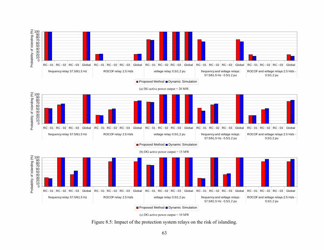
63

0102030405060708090

100

RC - 01 RC - 02 RC - 03 Global RC - 01 RC - 02 RC - 03 Global RC - 01 RC - 02 RC - 03 Global RC - 01 RC - 02 RC - 03 Global RC - 01 RC - 02 RC - 03 Global

frequency relay: 57.5/61.5 Hz ROCOF relay: 2.5 Hz/s voltage relay: 0.5/1.2 pu frequency and voltage relays:57.5/61.5 Hz - 0.5/1.2 pu

ROCOF and voltage relays:2.5 Hz/s -0.5/1.2 pu

Pro

babi

lity

of is

land

ing

(%)

Proposed Method Dynamic Simulation

(a) DG active power output = 20 MW.

0102030405060708090

100

RC - 01 RC - 02 RC - 03 Global RC - 01 RC - 02 RC - 03 Global RC - 01 RC - 02 RC - 03 Global RC - 01 RC - 02 RC - 03 Global RC - 01 RC - 02 RC - 03 Global

frequency relay: 57.5/61.5 Hz ROCOF relay: 2.5 Hz/s voltage relay: 0.5/1.2 pu frequency and voltage relays:57.5/61.5 Hz - 0.5/1.2 pu

ROCOF and voltage relays:2.5 Hz/s -0.5/1.2 pu

Pro

babi

lity

of is

land

ing

(%)

Proposed Method Dynamic Simulation

(b) DG active power output = 15 MW

0102030405060708090

100

RC - 01 RC - 02 RC - 03 Global RC - 01 RC - 02 RC - 03 Global RC - 01 RC - 02 RC - 03 Global RC - 01 RC - 02 RC - 03 Global RC - 01 RC - 02 RC - 03 Global

frequency relay: 57.5/61.5 Hz ROCOF relay: 2.5 Hz/s voltage relay: 0.5/1.2 pu frequency and voltage relays:57.5/61.5 Hz - 0.5/1.2 pu

ROCOF and voltage relays:2.5 Hz/s -0.5/1.2 pu

Pro

babi

lity

of is

land

ing

(%)

Proposed Method Dynamic Simulation

(c) DG active power output = 10 MW

Figure 8.5: Impact of the protection system relays on the risk of islanding.

64

0 200 400 600 800 1000 1200 1400 0

5

10

15

20

25

30

35

Time duration (min)

MW

/ M

VAr

period protected by the voltage relay

QG

QG + |ΔQ2|

PG

PG - |ΔP1|

PG + |ΔP2|

PLOAD

QLOAD

(a) load duration curve of RC-01.

0 200 400 600 800 1000 1200 1400 0

5

10

15

20

25

30

35

Time duration (min)

MW

/ M

VAr

period protected by the frequency relay

QG

QG + |ΔQ2|

PG

PG - |ΔP1|

PG + |ΔP2|

PLOAD

QLOAD

(b) load duration curve of RC-02.

Figure 8.6: Comparison of the non-detection periods associated with different relays (DG active power output = 20 MW; frequency relay 57.5/61.5 Hz; voltage relay 0.5/1.2 pu).

8.3.2 Relay Settings

In this section, the impact of the relay settings is analyzed. The idea is to compare the risk indexes derived from non-sensitive relay settings with those derived from sensitive settings. Note that sensitive settings give a smaller non-detection zone but has a higher chance to cause false alarm. The results are summarized in Figure 8.7 and Figure 8.8 for the cases of frequency and voltage relays, and ROCOF and voltage relays, respectively. The results show that relay settings have a significant impact on the risk index. A sensitive setting results in much smaller risk levels.

This finding can be understood using Figure 8.9, where one can see that the bands around the active and reactive power produced by the generator due to the NDZ decrease when the relay setting is adjusted more sensitive. When the load duration curve is flat around the DG generation level, a small change of the relay NDZ can result in significant change on the risk periods.

65

0102030405060708090

100

RC - 01 RC - 02 RC - 03 Global RC - 01 RC - 02 RC - 03 Global RC - 01 RC - 02 RC - 03 Global

20 MW 15 MW 10 MWDG power output

Pro

babi

lity

of is

land

ing

(%)

Proposed Method Dynamic Simulation

(a) frequency and voltage relay (57.5/61.5 Hz – 0.5/1.2 pu): non-sensitive settings.

0102030405060708090

100

RC - 01 RC - 02 RC - 03 Global RC - 01 RC - 02 RC - 03 Global RC - 01 RC - 02 RC - 03 Global

20 MW 15 MW 10 MWDG power output

Pro

babi

lity

of is

land

ing

(%)

Proposed Method Dynamic Simulation

(b) frequency and voltage relay (59.5/60.5 Hz – 0.7/1.15 pu): sensitive settings.

Figure 8.7: Impact of the relay setting on risk of islanding (frequency and voltage relay).

66

0102030405060708090

100

RC - 01 RC - 02 RC - 03 Global RC - 01 RC - 02 RC - 03 Global RC - 01 RC - 02 RC - 03 Global

20 MW 15 MW 10 MWDG power output

Pro

babi

lity

of is

land

ing

(%)

Proposed Method Dynamic Simulation

(a) ROCOF and voltage relay (2.5 Hz/s – 0.5/1.2 pu): non-sensitive settings.

0102030405060708090

100

RC - 01 RC - 02 RC - 03 Global RC - 01 RC - 02 RC - 03 Global RC - 01 RC - 02 RC - 03 Global

20 MW 15 MW 10 MWDG power output

Pro

babi

lity

of is

land

ing

(%)

Proposed Method Dynamic Simulation

(b) ROCOF and voltage relay (0.5 Hz/s – 0.7/1.15 pu): sensitive settings.

Figure 8.8: Impact of the relay setting on risk of islanding (ROCOF and voltage relay).

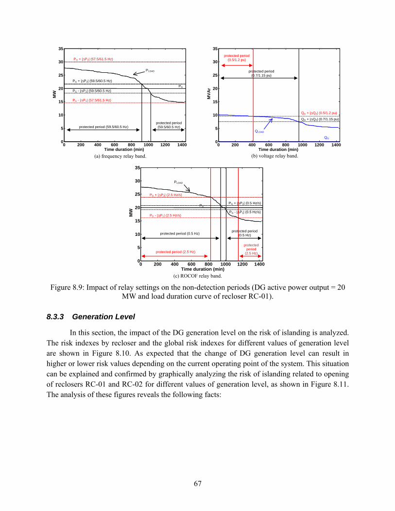
67

0 200 400 600 800 1000 1200 1400 0

5

10

15

20

25

30

35

Time duration (min)

MW

protected period (59.5/60.5 Hz)

PG

PG - |ΔP1| (59.5/60.5 Hz)

PG + |ΔP2| (59.5/60.5 Hz)

PLOAD

protected period (59.5/60.5 Hz)

PG - |ΔP1| (57.5/61.5 Hz)

PG + |ΔP2| (57.5/61.5 Hz)

(a) frequency relay band.

0 200 400 600 800 1000 1200 1400 0

5

10

15

20

25

30

35

Time duration (min)

MVA

r

protected period (0.5/1.2 pu)

QG

QG + |ΔQ2| (0.7/1.15 pu)

QLOAD

QG + |ΔQ2| (0.5/1.2 pu)

protected period (0.7/1.15 pu)

(b) voltage relay band.

0 200 400 600 800 1000 1200 1400 0

5

10

15

20

25

30

35

Time duration (min)

MW

protected period (2.5 Hz)

PG

PG - |ΔP1| (0.5 Hz/s)

PG + |ΔP2| (0.5 Hz/s)

PLOAD

PG - |ΔP1| (2.5 Hz/s)

PG + |ΔP2| (2.5 Hz/s)

protected period

(2.5 Hz)

protected period (0.5 Hz)protected period

(0.5 Hz)

(c) ROCOF relay band.

Figure 8.9: Impact of relay settings on the non-detection periods (DG active power output = 20 MW and load duration curve of recloser RC-01).

8.3.3 Generation Level

In this section, the impact of the DG generation level on the risk of islanding is analyzed. The risk indexes by recloser and the global risk indexes for different values of generation level are shown in Figure 8.10. As expected that the change of DG generation level can result in higher or lower risk values depending on the current operating point of the system. This situation can be explained and confirmed by graphically analyzing the risk of islanding related to opening of reclosers RC-01 and RC-02 for different values of generation level, as shown in Figure 8.11. The analysis of these figures reveals the following facts:

68

0102030405060708090

100

RC - 01 RC - 02 RC - 03 Global RC - 01 RC - 02 RC - 03 Global RC - 01 RC - 02 RC - 03 Global

20 MW 15 MW 10 MWDG power output

Pro

babi

lity o

f isl

andi

ng (%

)

Proposed Method Dynamic Simulation

(a) frequency and voltage relays: 57.5/61.5 Hz – 0.5/1.2 pu.

0102030405060708090

100

RC - 01 RC - 02 RC - 03 Global RC - 01 RC - 02 RC - 03 Global RC - 01 RC - 02 RC - 03 Global

20 MW 15 MW 10 MW

DG power output

Prob

abilit

y of

isla

ndin

g (%

)

Proposed Method Dynamic Simulation

(a) ROCOF and voltage relays: 2.5 Hz/s – 0.5/1.2 pu.

Figure 8.10: Impact of the generation level on the risk of islanding.

• Figure 8.11(a), (b), and (c) – recloser RC-01: When the generation level is 20 MW in this case (Figure 8.11(a)), the frequency relay is inefficient to detect the islanding situation since the active power generation level is situated between the maximum and minimum active power demand and the NDZ band contains the entire active load duration curve. In this situation, the protected period is due to the presence of the voltage relay, since the reactive power generation is much lower than the reactive power demand, lower enough to activate the relay. When the generation level decreases to 15 MW (Figure 8.11(b)), the frequency relay is able to detect the islanding situation during the period of high and medium demand, since the generation level is around the minimum demand value. With relation to the voltage relay, there is no difference when compared to the previous situation since the reactive power generation level is kept constant. When the active power generation level is reduced to 10 MW (Figure 8.11(c)), the frequency relay is able to detect the islanding situation for a wider time interval, since the generation level is lower than the minimum demand. Note that as the

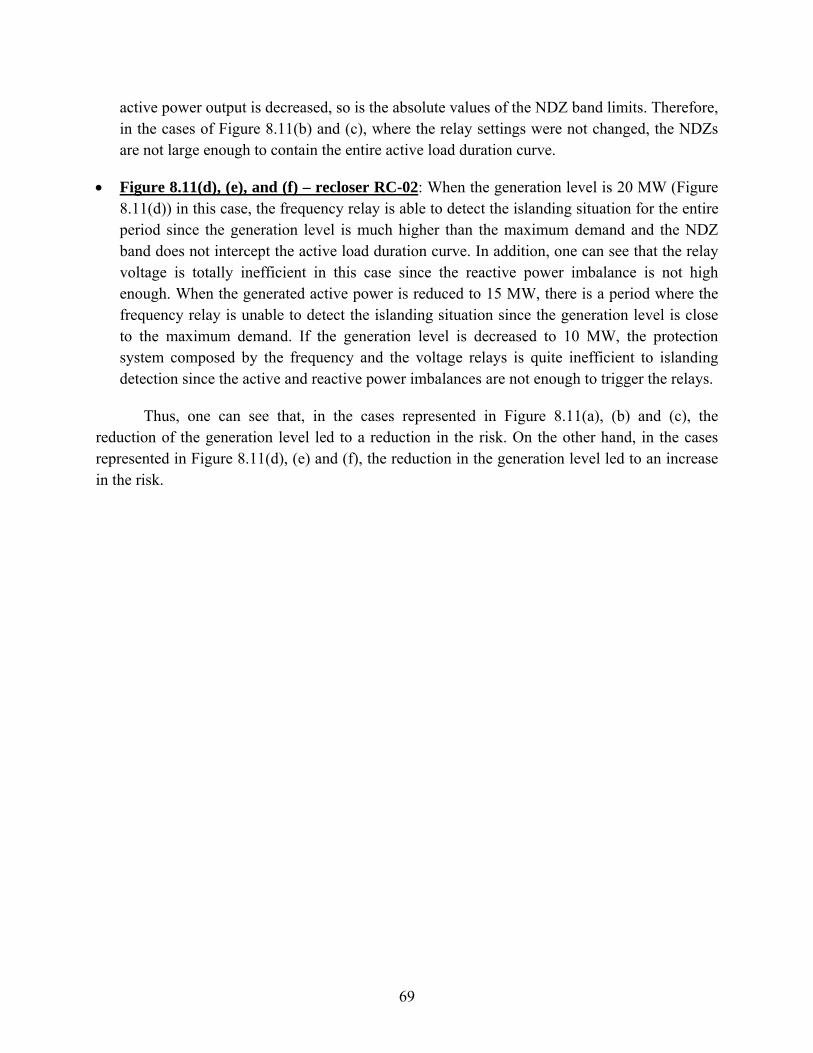
69

active power output is decreased, so is the absolute values of the NDZ band limits. Therefore, in the cases of Figure 8.11(b) and (c), where the relay settings were not changed, the NDZs are not large enough to contain the entire active load duration curve.

• Figure 8.11(d), (e), and (f) – recloser RC-02: When the generation level is 20 MW (Figure 8.11(d)) in this case, the frequency relay is able to detect the islanding situation for the entire period since the generation level is much higher than the maximum demand and the NDZ band does not intercept the active load duration curve. In addition, one can see that the relay voltage is totally inefficient in this case since the reactive power imbalance is not high enough. When the generated active power is reduced to 15 MW, there is a period where the frequency relay is unable to detect the islanding situation since the generation level is close to the maximum demand. If the generation level is decreased to 10 MW, the protection system composed by the frequency and the voltage relays is quite inefficient to islanding detection since the active and reactive power imbalances are not enough to trigger the relays.

Thus, one can see that, in the cases represented in Figure 8.11(a), (b) and (c), the reduction of the generation level led to a reduction in the risk. On the other hand, in the cases represented in Figure 8.11(d), (e) and (f), the reduction in the generation level led to an increase in the risk.

70

0 200 400 600 800 1000 1200 1400 0

5

10

15

20

25

30

35

Time duration (min)

MW

/ M

VAr

protected period

QG

QG + |ΔQ2|

PG

PG - |ΔP1|

PG + |ΔP2|

PLOAD

QLOAD

(a) DG power output = 20 MW and load duration curve of RC-01

0 200 400 600 800 1000 1200 1400 0

5

10

15

20

25

30

35

Time duration (min)

MW

/ MVA

r

protected period

QG

QG + |ΔQ2|

PG

PG - |ΔP1|

PG + |ΔP2|

PLOAD

QLOAD

(d) DG power output = 20 MW and load duration curve of RC-02

0 200 400 600 800 1000 1200 1400 0

5

10

15

20

25

30

35

Time duration (min)

MW

/ M

VAr protected period

QG

QG + |ΔQ2|

PG

PG - |ΔP1|

PG + |ΔP2|

PLOAD

QLOAD

protected period

(b) DG power output = 15 MW and load duration curve of RC-01

0 200 400 600 800 1000 1200 1400 0

5

10

15

20

25

30

35

Time duration (min)

MW

/ M

VAr

protected period

QG

QG + |ΔQ2|

PG

PG - |ΔP1|

PG + |ΔP2|

PLOAD

QLOAD

(e) DG power output = 15 MW and load duration curve of RC-02

0 200 400 600 800 1000 1200 1400 0

5

10

15

20

25

30

35

Time duration (min)

MW

/ M

VAr

protected period

QG

QG + |ΔQ2| PG

PG - |ΔP1|

PG + |ΔP2|

PLOAD

QLOAD

protected period

(c) DG power output = 10 MW and load duration curve of RC-01

0 200 400 600 800 1000 1200 1400 0

5

10

15

20

25

30

35

Time duration (min)

MW

/ M

VAr

QG + |ΔQ2| PG

PG - |ΔP1|

PG + |ΔP2|

PLOAD

QLOAD

(f) DG power output = 10 MW and load duration curve of RC-02

Figure 8.11: Graphical analysis of the impact of generation level on the risk of islanding (frequency relay 57.5/61.5 Hz; voltage relay 0.5/1.2 pu)).

8.3.4 Generator Size

In this section, the impact of the generator size (capacity) on the risk of islanding is analyzed. It is worth stressing that the look-up tables were built regardless of the generator size;

71

thus they can be promptly applied to any generator size. The generator size was selected as 30 MVA; 20 MVA and 10 MVA. Moreover, the analysis was conducted considering two levels of generation, which were selected as 20 MW and 10 MW. In the case of 20 MW generation level, only the generators with 30 MVA and 20 MVA were analyzed. The results are summarized in Figure 8.12 and Figure 8.13.

0102030405060708090

100

RC - 01 RC - 02 RC - 03 Global RC - 01 RC - 02 RC - 03 Global

30 MVA 20 MVADG size

Pro

babi

lity o

f isl

andi

ng (%

)

Proposed Method Dynamic Simulation

(a) DG power output = 20 MW

0102030405060708090

100

RC - 01 RC - 02 RC - 03 Global RC - 01 RC - 02 RC - 03 Global RC - 01 RC - 02 RC - 03 Global

30 MVA 20 MVA 10 MVADG size

Prob

abilit

y of

isla

ndin

g (%

)

Proposed Method Dynamic Simulation

(b) DG power output = 10 MW

Figure 8.12: Impact of the generator size on the risk of islanding (frequency and voltage relays: 57.5/61.5 Hz – 0.5/1.2 pu).

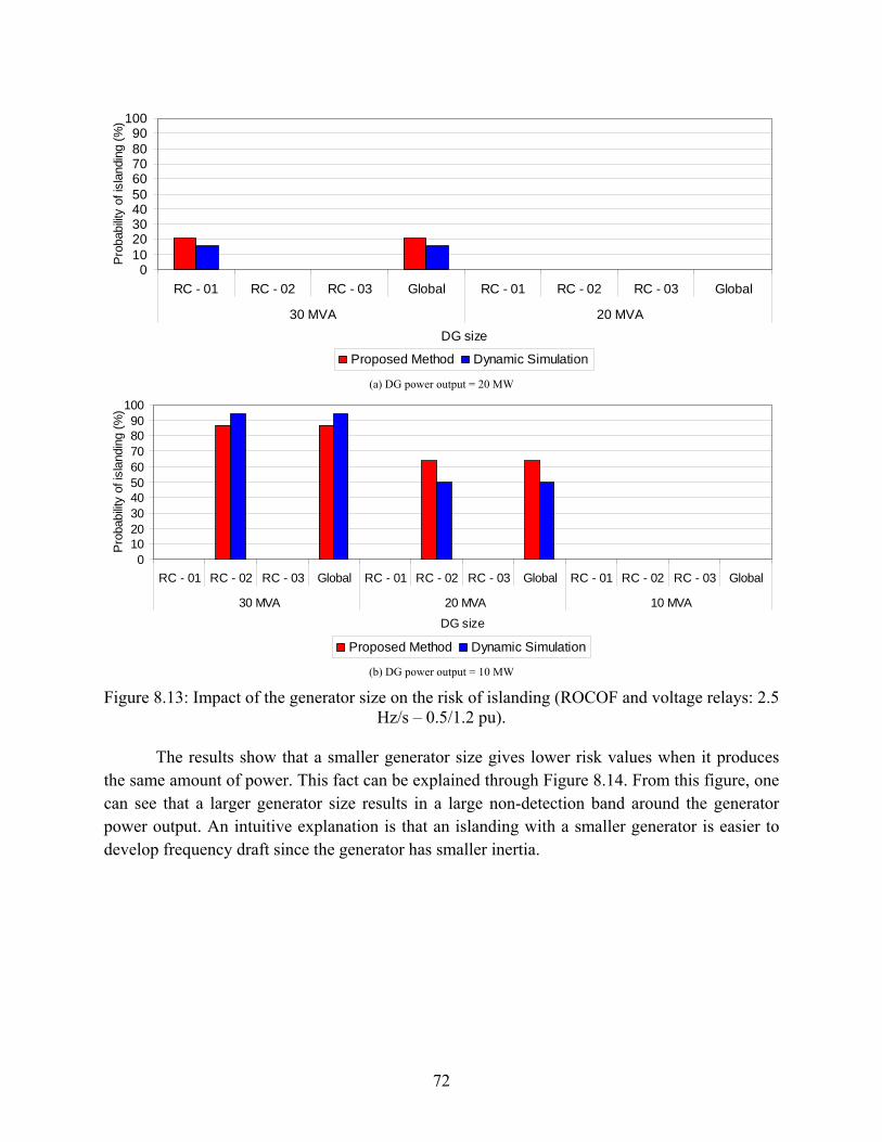
72

0102030405060708090

100

RC - 01 RC - 02 RC - 03 Global RC - 01 RC - 02 RC - 03 Global

30 MVA 20 MVADG size

Pro

babi

lity o

f isl

andi

ng (%

)

Proposed Method Dynamic Simulation

(a) DG power output = 20 MW

0102030405060708090

100

RC - 01 RC - 02 RC - 03 Global RC - 01 RC - 02 RC - 03 Global RC - 01 RC - 02 RC - 03 Global

30 MVA 20 MVA 10 MVADG size

Prob

abilit

y of

isla

ndin

g (%

)

Proposed Method Dynamic Simulation

(b) DG power output = 10 MW

Figure 8.13: Impact of the generator size on the risk of islanding (ROCOF and voltage relays: 2.5 Hz/s – 0.5/1.2 pu).

The results show that a smaller generator size gives lower risk values when it produces the same amount of power. This fact can be explained through Figure 8.14. From this figure, one can see that a larger generator size results in a large non-detection band around the generator power output. An intuitive explanation is that an islanding with a smaller generator is easier to develop frequency draft since the generator has smaller inertia.

73

0 200 400 600 800 1000 1200 1400 0

5

10

15

20

25

30

35

Time duration (min)

MW

PG

PG - |ΔP1| (10 MVA)

PG + |ΔP2|(10 MVA) PLOAD

PG + |ΔP2|(20 MVA)

PG - |ΔP1| (20 MVA) PG - |ΔP1| (30 MVA)

PG + |ΔP2|(30 MVA)

protectedperiod

(20 MVA)

protected period (10 MVA)

(a) frequency relay protection (57.5/61.5 Hz).

0 200 400 600 800 1000 1200 1400 0

5

10

15

20

25

30

35

Time duration (min)

MVA

R

QG + |ΔQ2|(10 MVA)

QG + |ΔQ2|(20 MVA)

QG + |ΔQ2|(30 MVA)

protected period (10 MVA)

QLOAD

QG

(b) voltage relay protection (0.5/1.2 pu).

0 200 400 600 800 1000 1200 1400 0

5

10

15

20

25

30

35

Time duration (min)

MW

PG PG - |ΔP1| (10 MVA)

PG + |ΔP2|(10 MVA)

PLOAD

PG + |ΔP2|(20 MVA)

PG - |ΔP1| (20 MVA) PG - |ΔP1| (30 MVA)

PG + |ΔP2|(30 MVA)

protected period(20 MVA)

protected period (10 MVA)

protected period

(20 MVA)

protected period (10 MVA)

protectedperiod

(30 MVA)

(c) ROCOF relay protection (2.5 Hz).

Figure 8.14: Graphical analysis of the impact of the generator size on the risk of islanding (DG active power output = 10 MW and load duration curve of recloser RC-02).

8.3.5 Required Detection Time

In this section, the impact of the required detection time is investigated. Required detection time of 500 ms, 1000 ms and 1500 ms were analyzed. The results are summarized in Figure 8.15 and Figure 8.16 for the combination of a frequency and a voltage relay, and a ROCOF and a voltage relay, respectively. In addition, different combinations of relays settings were considered. The results related to the required detection time of 1500 ms are not presented since the risk of islanding is zero for all cases analyzed.

74

0102030405060708090

100

RC - 01 RC - 02 RC - 03 Global RC - 01 RC - 02 RC - 03 Global RC - 01 RC - 02 RC - 03 Global

20 MW 15 MW 10 MWDG size

Prob

abilit

y of

isla

ndin

g (%

)

Proposed Method Dynamic Simulation

(a) required detection time = 500 ms.

0102030405060708090

100

RC - 01 RC - 02 RC - 03 Global RC - 01 RC - 02 RC - 03 Global RC - 01 RC - 02 RC - 03 Global

20 MW 15 MW 10 MWDG size

Prob

abilit

y of

isla

ndin

g (%

)

Proposed Method Dynamic Simulation

(b) required detection time = 1000 ms.

Figure 8.15: Impact of the required detection time on the risk of islanding (Frequency and voltage relays: 57.5/61.5 Hz - 0.5/1.2 pu).

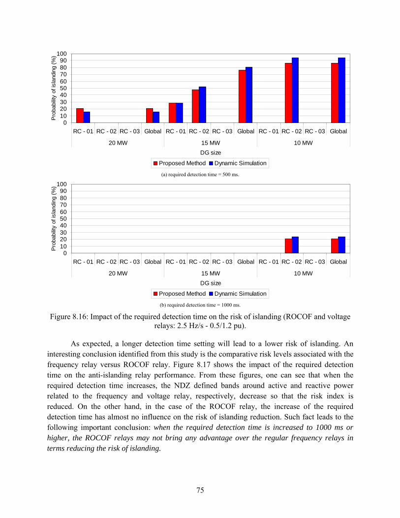
75

0102030405060708090

100

RC - 01 RC - 02 RC - 03 Global RC - 01 RC - 02 RC - 03 Global RC - 01 RC - 02 RC - 03 Global

20 MW 15 MW 10 MWDG size

Prob

abilit

y of

isla

ndin

g (%

)

Proposed Method Dynamic Simulation

(a) required detection time = 500 ms.

0102030405060708090

100

RC - 01 RC - 02 RC - 03 Global RC - 01 RC - 02 RC - 03 Global RC - 01 RC - 02 RC - 03 Global

20 MW 15 MW 10 MWDG size

Prob

abilit

y of

isla

ndin

g (%

)

Proposed Method Dynamic Simulation

(b) required detection time = 1000 ms.

Figure 8.16: Impact of the required detection time on the risk of islanding (ROCOF and voltage relays: 2.5 Hz/s - 0.5/1.2 pu).

As expected, a longer detection time setting will lead to a lower risk of islanding. An interesting conclusion identified from this study is the comparative risk levels associated with the frequency relay versus ROCOF relay. Figure 8.17 shows the impact of the required detection time on the anti-islanding relay performance. From these figures, one can see that when the required detection time increases, the NDZ defined bands around active and reactive power related to the frequency and voltage relay, respectively, decrease so that the risk index is reduced. On the other hand, in the case of the ROCOF relay, the increase of the required detection time has almost no influence on the risk of islanding reduction. Such fact leads to the following important conclusion: when the required detection time is increased to 1000 ms or higher, the ROCOF relays may not bring any advantage over the regular frequency relays in terms reducing the risk of islanding.

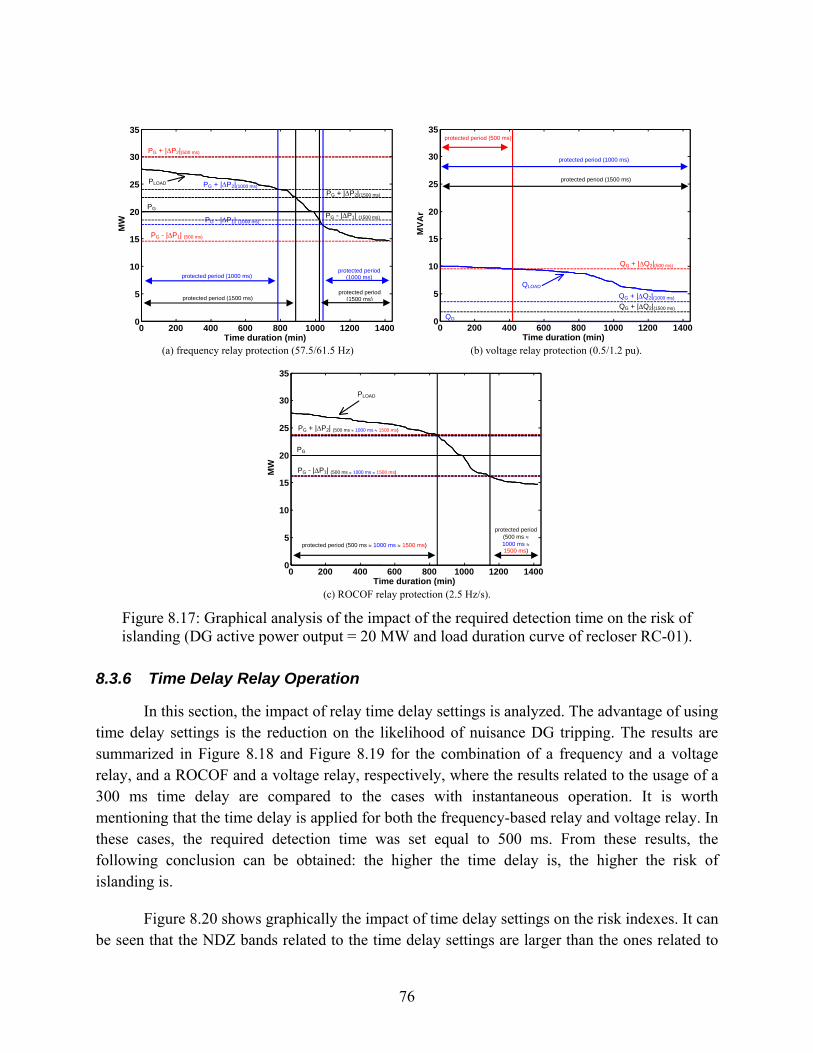
76

0 200 400 600 800 1000 1200 1400 0

5

10

15

20

25

30

35

Time duration (min)

MW

PG

PG - |ΔP1| (500 ms)

PG + |ΔP2|(500 ms)

PLOAD PG + |ΔP2|(1000 ms)

PG - |ΔP1| (1500 ms)

PG + |ΔP2|(1500 ms)

protected period (1500 ms)

protected period (1000 ms)

PG - |ΔP1| (1000 ms)

protected period (1000 ms)

protected period (1500 ms)

(a) frequency relay protection (57.5/61.5 Hz)

0 200 400 600 800 1000 1200 1400 0

5

10

15

20

25

30

35

Time duration (min)

MVA

r

QG + |ΔQ2|(500 ms)

QG + |ΔQ2|(1000 ms) QG + |ΔQ2|(1500 ms)

protected period (500 ms)

QLOAD

QG

protected period (1000 ms)

protected period (1500 ms)

(b) voltage relay protection (0.5/1.2 pu).

0 200 400 600 800 1000 1200 1400 0

5

10

15

20

25

30

35

Time duration (min)

MW

PG

PG - |ΔP1| (500 ms ≈ 1000 ms ≈ 1500 ms)

PLOAD

protected period (500 ms ≈ 1000 ms ≈ 1500 ms)

PG + |ΔP2| (500 ms ≈ 1000 ms ≈ 1500 ms)

protected period (500 ms ≈ 1000 ms ≈ 1500 ms)

(c) ROCOF relay protection (2.5 Hz/s).

Figure 8.17: Graphical analysis of the impact of the required detection time on the risk of islanding (DG active power output = 20 MW and load duration curve of recloser RC-01).

8.3.6 Time Delay Relay Operation

In this section, the impact of relay time delay settings is analyzed. The advantage of using time delay settings is the reduction on the likelihood of nuisance DG tripping. The results are summarized in Figure 8.18 and Figure 8.19 for the combination of a frequency and a voltage relay, and a ROCOF and a voltage relay, respectively, where the results related to the usage of a 300 ms time delay are compared to the cases with instantaneous operation. It is worth mentioning that the time delay is applied for both the frequency-based relay and voltage relay. In these cases, the required detection time was set equal to 500 ms. From these results, the following conclusion can be obtained: the higher the time delay is, the higher the risk of islanding is.

Figure 8.20 shows graphically the impact of time delay settings on the risk indexes. It can be seen that the NDZ bands related to the time delay settings are larger than the ones related to

77

the instantaneous settings. Thus, in spite of making the relays more stable against nuisance tripping, time delay settings may increase the islanding risks. However, in the case of ROCOF relay, such increase can be small.

0102030405060708090

100

RC - 01 RC - 02 RC - 03 Global RC - 01 RC - 02 RC - 03 Global RC - 01 RC - 02 RC - 03 Global

20 MW 15 MW 10 MWDG power output

Prob

abilit

y of

isla

ndin

g (%

)

Proposed Method Dynamic Simulation

(a) frequency and voltage relay (59.5/60.5 Hz and 0.8/1.2 pu – 300 ms)

0102030405060708090

100

RC - 01 RC - 02 RC - 03 Global RC - 01 RC - 02 RC - 03 Global RC - 01 RC - 02 RC - 03 Global

20 MW 15 MW 10 MWDG power output

Prob

abilit

y of

isla

ndin

g (%

)

Proposed Method Dynamic Simulation

(b) frequency and voltage relay (59.5/60.5 Hz and 0.8/1.2 pu – without time delay)

Figure 8.18: Impact of time delay relay operation on the risk of islanding (frequency and voltage relay and required detection time = 500 ms).

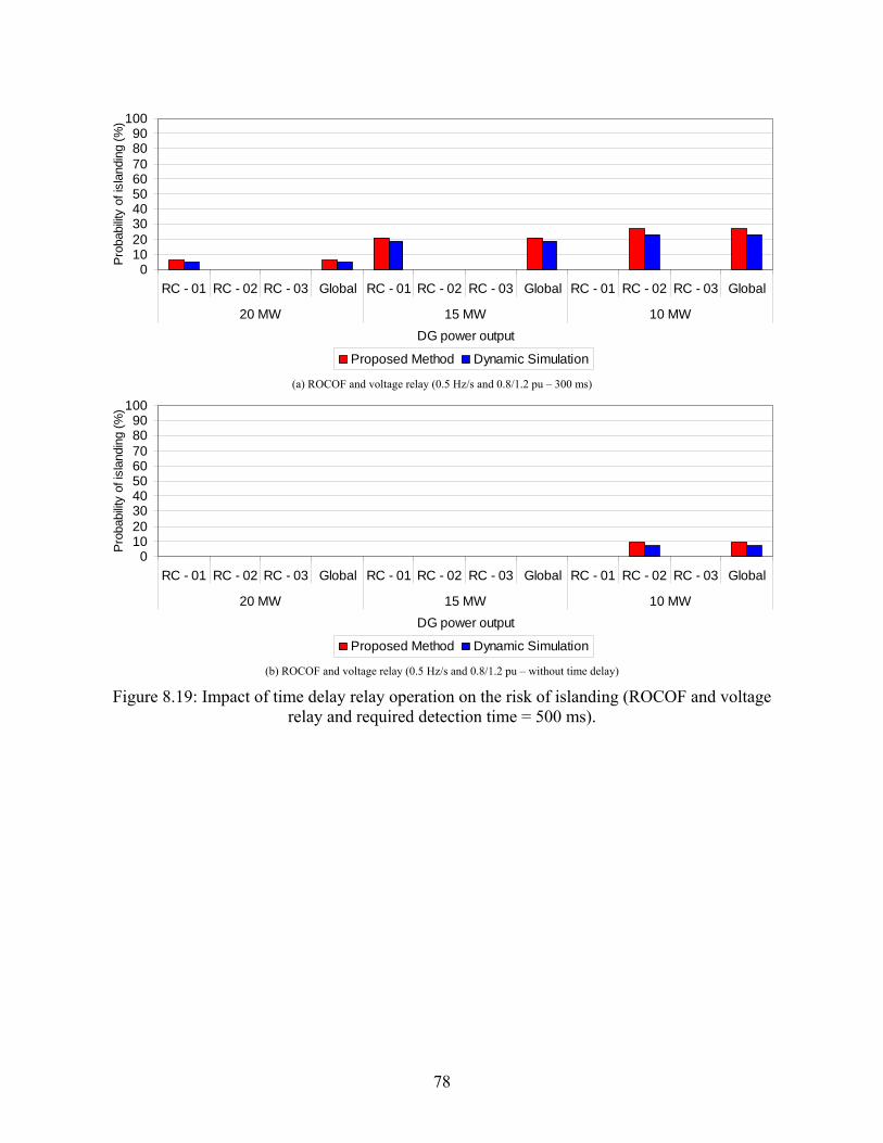
78

0102030405060708090

100

RC - 01 RC - 02 RC - 03 Global RC - 01 RC - 02 RC - 03 Global RC - 01 RC - 02 RC - 03 Global

20 MW 15 MW 10 MWDG power output

Prob

abilit

y of

isla

ndin

g (%

)

Proposed Method Dynamic Simulation

(a) ROCOF and voltage relay (0.5 Hz/s and 0.8/1.2 pu – 300 ms)

0102030405060708090

100

RC - 01 RC - 02 RC - 03 Global RC - 01 RC - 02 RC - 03 Global RC - 01 RC - 02 RC - 03 Global

20 MW 15 MW 10 MWDG power output

Prob

abilit

y of

isla

ndin

g (%

)

Proposed Method Dynamic Simulation

(b) ROCOF and voltage relay (0.5 Hz/s and 0.8/1.2 pu – without time delay)

Figure 8.19: Impact of time delay relay operation on the risk of islanding (ROCOF and voltage relay and required detection time = 500 ms).

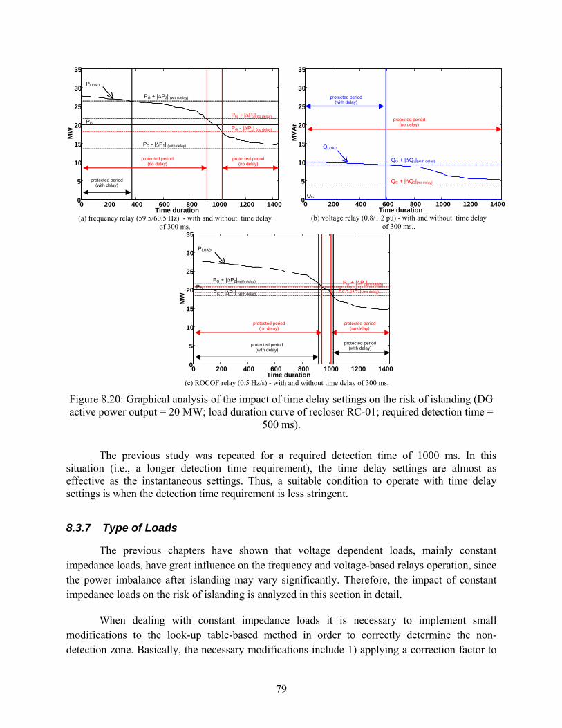
79

0 200 400 600 800 1000 1200 14000

5

10

15

20

25

30

35

Time duration

MW

PG - |ΔP1| (no delay)

PG + |ΔP2|(no delay)

PLOAD

PG - |ΔP1| (with delay)

PG + |ΔP2| (with delay)

protected period (no delay)

protected period (with delay)

protected period (no delay)

PG

(a) frequency relay (59.5/60.5 Hz) - with and without time delay of 300 ms.

0 200 400 600 800 1000 1200 14000

5

10

15

20

25

30

35

Time duration

MVA

r

QG + |ΔQ2|(no delay)

QLOAD

QG + |ΔQ2|(with delay)

protected period (with delay)

protected period (no delay)

QG

(b) voltage relay (0.8/1.2 pu) - with and without time delay of 300 ms..

0 200 400 600 800 1000 1200 14000

5

10

15

20

25

30

35

Time duration

MW

PG - |ΔP1| (no delay) PG + |ΔP2|(no delay)

PLOAD

PG - |ΔP1| (with delay)

PG + |ΔP2|(with delay)

protected period (no delay)

protected period (with delay)

protected period (no delay)

protected period (with delay)

PG

(c) ROCOF relay (0.5 Hz/s) - with and without time delay of 300 ms.

Figure 8.20: Graphical analysis of the impact of time delay settings on the risk of islanding (DG active power output = 20 MW; load duration curve of recloser RC-01; required detection time =

500 ms).

The previous study was repeated for a required detection time of 1000 ms. In this

situation (i.e., a longer detection time requirement), the time delay settings are almost as effective as the instantaneous settings. Thus, a suitable condition to operate with time delay settings is when the detection time requirement is less stringent.

8.3.7 Type of Loads

The previous chapters have shown that voltage dependent loads, mainly constant impedance loads, have great influence on the frequency and voltage-based relays operation, since the power imbalance after islanding may vary significantly. Therefore, the impact of constant impedance loads on the risk of islanding is analyzed in this section in detail.

When dealing with constant impedance loads it is necessary to implement small modifications to the look-up table-based method in order to correctly determine the non-detection zone. Basically, the necessary modifications include 1) applying a correction factor to

80

the limits ΔQ1 and ΔQ2 and 2) adopting axis rotation to the active and reactive power variables. Such modifications are explained in detail in Appendix D. Once the modified non-detection zone is obtained, the proposed method can be applied to systems with constant impedance loads.

8.3.7.1 Validation of risk results in the presence of constant impedance loads

The results obtained by the proposed method are compared with those obtained with intensive dynamic simulation first. The results shown in Figure 8.21 suggest that the risk indexes calculated by the proposed method match very well the one calculated by intensive dynamic simulations. It must be stressed that cases considering other relay settings, different detection time frames and generator sizes were also analyzed and similar accuracy has been obtained, but only two representative cases are presented.

0102030405060708090

100

RC - 01 RC - 02 RC - 03 Global RC - 01 RC - 02 RC - 03 Global RC - 01 RC - 02 RC - 03 Global

20 MW 15 MW 10 MWDG power output

Pro

babi

lity o

f isl

andi

ng (%

)

Proposed Method Dynamic Simulation

(a) frequency and voltage relay (57.5/61.5 Hz and 0.5/1.2 pu )

0102030405060708090

100

RC - 01 RC - 02 RC - 03 Global RC - 01 RC - 02 RC - 03 Global RC - 01 RC - 02 RC - 03 Global

20 MW 15 MW 10 MWDG power output

Pro

babi

lity o

f isl

andi

ng (%

)

Proposed Method Dynamic Simulation

(b) ROCOF and voltage relay (2.5 Hz/s and 0.5/1.2 pu)

Figure 8.21 – Analysis of constant impedance loads (required detection time = 500 ms).

81

8.3.7.2 Comparative analysis for constant power and constant impedance loads

This section presents a comparative analysis between the risks of unintentional islanding with constant power loads versus constant impedance loads. Two representative results are shown in Figure 8.22, one for a combination of frequency and voltage relays and another one for a combination of ROCOF and voltage relays. It can be seen that there are situations where the risk associated with the constant impedance loads is higher than those with the constant power loads. However, in other situations, the risk associated with the constant impedance loads is lower than the risk with the constant power loads.

0102030405060708090

100

RC - 01 RC - 02 RC - 03 Global RC - 01 RC - 02 RC - 03 Global RC - 01 RC - 02 RC - 03 Global

20 MW 15 MW 10 MWDG power output

Prob

abilit

y of

isla

ndin

g (%

)

Constant Impedance Constant Power

(a) frequency and voltage relay (57.5/61.5 Hz and 0.5/1.2 pu )

0102030405060708090

100

RC - 01 RC - 02 RC - 03 Global RC - 01 RC - 02 RC - 03 Global RC - 01 RC - 02 RC - 03 Global

20 MW 15 MW 10 MWDG power output

Prob

abilit

y of

isla

ndin

g (%

)

Constant Impedance Constant Power

(b) ROCOF and voltage relay (2.5 Hz/s and 0.5/1.2 pu)

Figure 8.22 – Risk of islanding comparative analysis: constant power and constant impedance loads (required detection time = 500 ms).

This behavior can be explained using the non-detection zones of different load types shown in Figure 8.23. It can be seen that depending on the combination of excess/deficit of

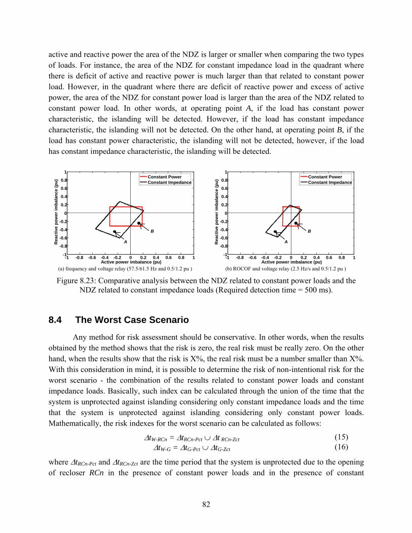
82

active and reactive power the area of the NDZ is larger or smaller when comparing the two types of loads. For instance, the area of the NDZ for constant impedance load in the quadrant where there is deficit of active and reactive power is much larger than that related to constant power load. However, in the quadrant where there are deficit of reactive power and excess of active power, the area of the NDZ for constant power load is larger than the area of the NDZ related to constant power load. In other words, at operating point A, if the load has constant power characteristic, the islanding will be detected. However, if the load has constant impedance characteristic, the islanding will not be detected. On the other hand, at operating point B, if the load has constant power characteristic, the islanding will not be detected, however, if the load has constant impedance characteristic, the islanding will be detected.

-1 -0.8 -0.6 -0.4 -0.2 0 0.2 0.4 0.6 0.8 1-1 -0.8 -0.6 -0.4 -0.2

0 0.2 0.4 0.6 0.8

1

Active power imbalance (pu)

Rea

ctiv

e po

wer

imba

lanc

e (p

u) Constant Power

Constant Impedance

A

B

(a) frequency and voltage relay (57.5/61.5 Hz and 0.5/1.2 pu )

-1 -0.8 -0.6 -0.4 -0.2 0 0.2 0.4 0.6 0.8 1-1

-0.8

-0.6

-0.4

-0.2

0

0.2

0.4

0.6

0.8

1

Active power imbalance (pu)

Rea

ctiv

e po

wer

imba

lanc

e (p

u) Constant Power

Constant Impedance

A

B

(b) ROCOF and voltage relay (2.5 Hz/s and 0.5/1.2 pu )

Figure 8.23: Comparative analysis between the NDZ related to constant power loads and the NDZ related to constant impedance loads (Required detection time = 500 ms).

8.4 The Worst Case Scenario

Any method for risk assessment should be conservative. In other words, when the results obtained by the method shows that the risk is zero, the real risk must be really zero. On the other hand, when the results show that the risk is X%, the real risk must be a number smaller than X%. With this consideration in mind, it is possible to determine the risk of non-intentional risk for the worst scenario - the combination of the results related to constant power loads and constant impedance loads. Basically, such index can be calculated through the union of the time that the system is unprotected against islanding considering only constant impedance loads and the time that the system is unprotected against islanding considering only constant power loads. Mathematically, the risk indexes for the worst scenario can be calculated as follows:

ΔtW-RCn = ΔtRCn-Pct ∪ Δt RCn-Zct (15) ΔtW-G = ΔtG-Pct ∪ ΔtG-Zct (16)

where ΔtRCn-Pct and ΔtRCn-Zct are the time period that the system is unprotected due to the opening of recloser RCn in the presence of constant power loads and in the presence of constant

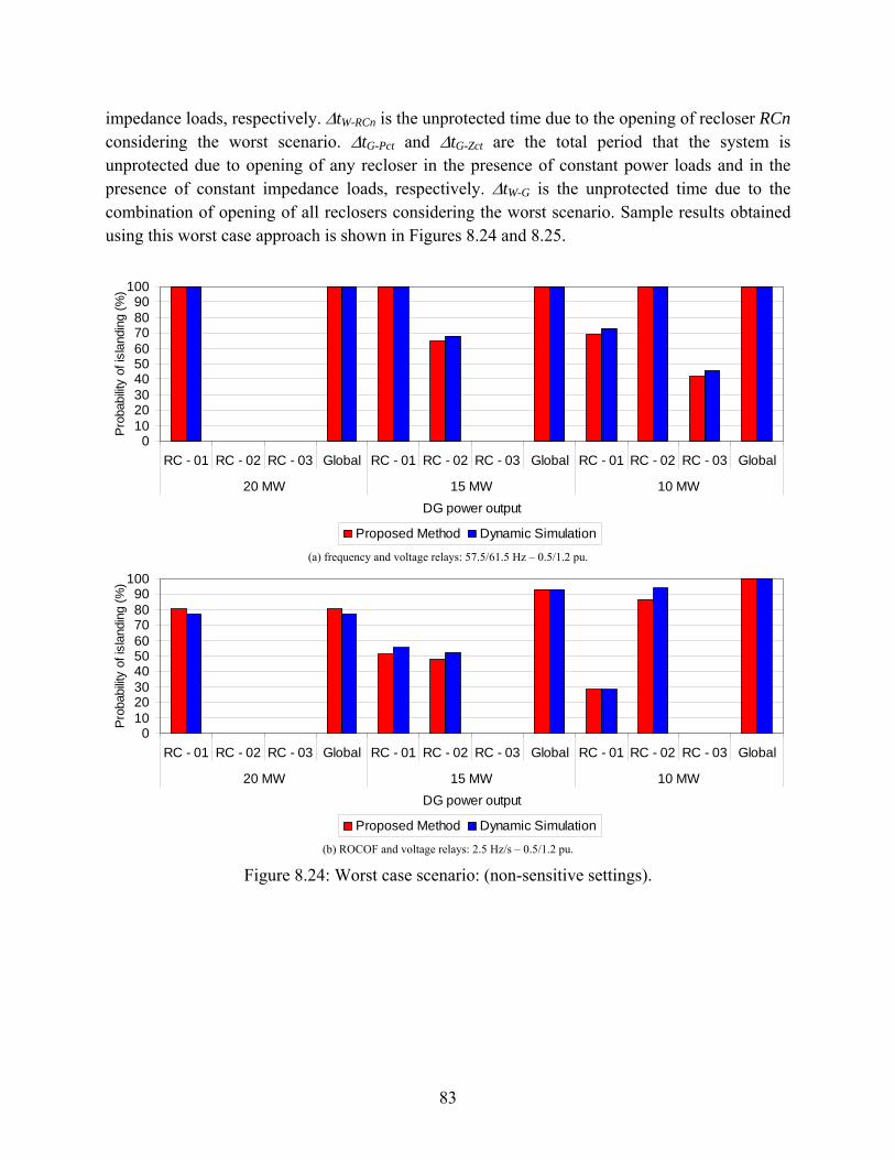
83

impedance loads, respectively. ΔtW-RCn is the unprotected time due to the opening of recloser RCn considering the worst scenario. ΔtG-Pct and ΔtG-Zct are the total period that the system is unprotected due to opening of any recloser in the presence of constant power loads and in the presence of constant impedance loads, respectively. ΔtW-G is the unprotected time due to the combination of opening of all reclosers considering the worst scenario. Sample results obtained using this worst case approach is shown in Figures 8.24 and 8.25.

0102030405060708090

100

RC - 01 RC - 02 RC - 03 Global RC - 01 RC - 02 RC - 03 Global RC - 01 RC - 02 RC - 03 Global

20 MW 15 MW 10 MWDG power output

Prob

abilit

y of

isla

ndin

g (%

)

Proposed Method Dynamic Simulation

(a) frequency and voltage relays: 57.5/61.5 Hz – 0.5/1.2 pu.

0102030405060708090

100

RC - 01 RC - 02 RC - 03 Global RC - 01 RC - 02 RC - 03 Global RC - 01 RC - 02 RC - 03 Global

20 MW 15 MW 10 MWDG power output

Prob

abilit

y of

isla

ndin

g (%

)

Proposed Method Dynamic Simulation

(b) ROCOF and voltage relays: 2.5 Hz/s – 0.5/1.2 pu.

Figure 8.24: Worst case scenario: (non-sensitive settings).

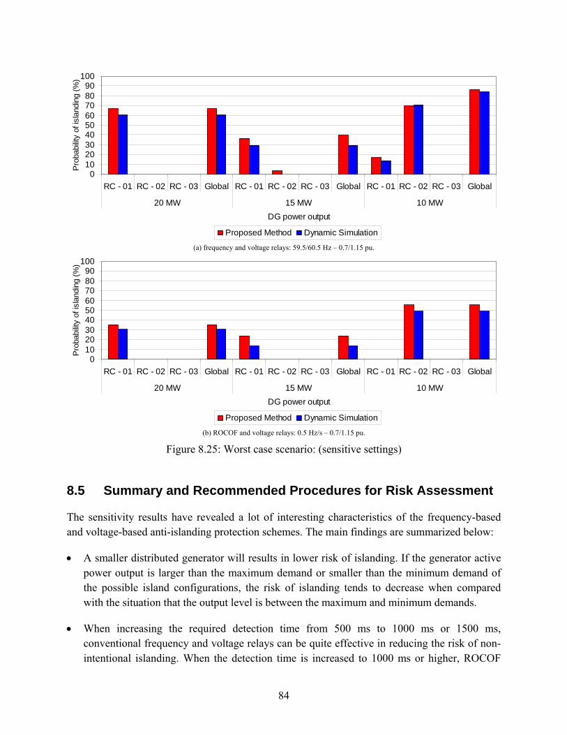
84

0102030405060708090

100

RC - 01 RC - 02 RC - 03 Global RC - 01 RC - 02 RC - 03 Global RC - 01 RC - 02 RC - 03 Global

20 MW 15 MW 10 MWDG power output

Prob

abilit

y of

isla

ndin

g (%

)

Proposed Method Dynamic Simulation

(a) frequency and voltage relays: 59.5/60.5 Hz – 0.7/1.15 pu.

0102030405060708090

100

RC - 01 RC - 02 RC - 03 Global RC - 01 RC - 02 RC - 03 Global RC - 01 RC - 02 RC - 03 Global

20 MW 15 MW 10 MWDG power output

Prob

abilit

y of

isla

ndin

g (%

)

Proposed Method Dynamic Simulation

(b) ROCOF and voltage relays: 0.5 Hz/s – 0.7/1.15 pu.

Figure 8.25: Worst case scenario: (sensitive settings)

8.5 Summary and Recommended Procedures for Risk Assessment

The sensitivity results have revealed a lot of interesting characteristics of the frequency-based and voltage-based anti-islanding protection schemes. The main findings are summarized below:

• A smaller distributed generator will results in lower risk of islanding. If the generator active power output is larger than the maximum demand or smaller than the minimum demand of the possible island configurations, the risk of islanding tends to decrease when compared with the situation that the output level is between the maximum and minimum demands.

• When increasing the required detection time from 500 ms to 1000 ms or 1500 ms, conventional frequency and voltage relays can be quite effective in reducing the risk of non-intentional islanding. When the detection time is increased to 1000 ms or higher, ROCOF

85

relays may not bring any advantage over the regular frequency relays with respective to the islanding risk level.

• Time delay settings of frequency-based and voltage relays can increase the risk of non-intentional islanding. Nevertheless, at high-required detection times (1000 ms or higher) their use can be quite attractive, since the risk of islanding is reduced to the levels associated with instantaneous settings, and relays false operation can be minimized.

• The load characteristics can influence the risk of islanding significantly. The most conservative situations, which lead to higher risk indexes, are related to both constant impedance and constant power loads. Thus, a worst-case scenario can be established by combining the influences of both types of loads in the proposed method, as explained in Section 8.4.

The results also reveal that it is not practical to draw general conclusions regarding the islanding risk levels of a synchronous DG scheme. A more sound approach is to develop an easy-to-use method for risk assessment. The proposed lookup table based method has shown to be effective in accomplishing this goal. The method is further summarized below by taking into account the most conservative cases:

• STEP 1: Build, from the daily load curves, the load duration curves of active and reactive power demands. If the generator exciter is voltage-controlled or there are only frequency-based relays in the anti-islanding protection system, the reactive load duration curves can be neglected.

• STEP 2: Determine the active and reactive NDZ bands by using the lookup tables presented in Section 7, the relays settings and the required detection time.

• STEP 3: Find the unprotected time periods for different reclosers and the total unprotected time period, by using the methodology explained in Section 7.

• STEP 4: Repeat Steps 2 and 3 to constant power loads and to constant impedance loads;

• STEP 5: Determined the unprotected time periods for reclosers and the total unprotected time period by combining the results related to constant power loads and constant impedance loads as explained in Section 8.4

It is worth pointing out that the above method can be easily programmed on Excel or other computing platforms.

86

CHAPTER 9: CONCLUSIONS

Non-intentional islanding of distributed generators occurs when the anti-islanding protection fails to detect the islanding faster than the detection time required by the host utility. The impact caused by non-intentional islanding of distributed synchronous generators is more serious than the impact caused by non-intentional islanding of photovoltaic (PV) systems. This is because the synchronous DGs typically have much larger size and are connected to the medium voltage networks equipped with automatic reclosers. By the same reasons, evaluating the risk of islanding of distributed synchronous generators is not a simple process. Due to the large variety of feeder loads that a synchronous generator can supply and the presence of reclosers in the distribution grids, many distinct conditions of load-generation balance may occur, which result in different performances of the anti-islanding devices. Moreover, our results have shown that the risk of islanding are dependent on the relay type and setting, generator size, generator output level, required detection time and system load type.

In view of the variety of islanding scenarios involving synchronous DGs, this project has developed a set of tools to facilitate the estimation of the risk of non-intentional islanding on a case by case basis by utility engineers, as it is not practical to produce typical probability risk values that can be applied to all DG interconnection cases. The method was developed and applied to frequency-based and voltage-based relays since, at present, they are first choice for anti-islanding protection adopted by the power industry. Typical values of detection time required from 500 ms to 1500 ms were used to develop the method. The cause of islanding formation considered here was the opening of feeder reclosers. The fuse-blowing and other open conductor caused islanding scenarios were not considered here but can be included by the proposed method.

The proposed method is based on the fact that the risk of islanding formation is essentially the probability of a DG-containing distribution system entering the non-detection zone (NDZ) created by the anti-islanding devices. The NDZ defines bands around the power produced by the DG on the active/reactive power versus time plan. Consequently, this analysis needs data on the non-detection zones of the anti-islanding relays. As shown in the report, the non-detection zones of typical anti-islanding relays are dependent on the voltage-dependent characteristics of the loads and the voltage control characteristics of the generator. Furthermore, the shape of the non-detection zones is not quite rectangular. All these factors can complicate the task of risk assessment considerably. The approach proposed by this project was to use look-up tables representing conservative rectangular non-detection zones to calculate the risk of non-intentional islanding. The method is simple and can be easily programmed on Excel or other computing platforms.

87

Based on extensive case studies and theoretical analysis conducted by this project, the main findings on the characteristics of non-intentional islanding of synchronous generators are summarized below:

• The combination of frequency-based and voltage relays can reduce the risk of islanding if the distributed synchronous generator exciter is configured to control reactive power output. Otherwise (i.e., when the excitation system is used to voltage control), the voltage relay will become ineffective to detect islanding and the risks of non-detection are related to the frequency-based relays only. Consequently, if the generator controls terminal voltage, it is necessary to consider only the active power duration curve in the proposed methodology.

• If the generator active power output is larger than the maximum active power demand or smaller than the minimum active power demand considering all possibilities of island formations, the risk of islanding tends to decrease in comparison to the case that the active power output level is between the maximum and minimum power demands.

• Small synchronous generators will result in smaller risks of islanding than large ones, since the corresponding non-detection zones are also smaller.

• The vector surge relay does not offer additional advantages over the frequency relay for anti-islanding protection. The relay exhibits the same islanding detection characteristics as that of the frequency relay. As a result, there is no need to install a dedicated VSR for anti-islanding application because a frequency relay, which is normally required for any DG installation, is as effective as the vector surge relay for anti-islanding application.

• In general, as the required detection time is increased, the risk of islanding decreases. However, an important behavior of ROCOF relays was observed: due to their operating characteristic, which present an abrupt increase of the detection time for low levels of active power imbalance, required detection times equal or larger than 1000 ms do not cause reduction of the risk of islanding, if compared to frequency relays.

• Time delay settings of frequency-based and voltage relays can increase the risk of islanding. However, if the required detection time is equal or larger than 1000 ms, the relays performances with time delay and instantaneous settings are similar. Therefore, with high-required detection times (1000 ms or higher), time delay settings can be quite attractive, since the risk of islanding is reduced to the levels associated with instantaneous settings and relays false operation can be minimized.

• The load type can affect significantly the risk of islanding, depending on the combinations of excess and deficit of active and reactive powers in the islanded system. Thus, the worst case scenario was defined as the one considering the combination of the

88

non-detection zones related constant power and constant impedance load types. Such scenario leads to conservative risk of islanding values.

89

CHAPTER 10: REFERENCES

[1] ANSI/IEEE, IEEE Guide for Interfacing Dispersed Storage and Generation Facilities with Electric Utility Systems, IEEE/ANSI Std., 1988.

[2] IEEE standard for interconnecting distributed resources with electric power systems, IEEE Standard P1547, 2003.

[3] Electricity Association, G75/1, Recommendations for the Connection of Embedded Generating Plant to Public Distribution Systems above 20 kV or with Outputs over 5 MW, Electricity Association Standard G75/1, 2003

[4] W. Bower and M. Ropp, Evaluation of Islanding Detection Methods for Photovoltaic Utility. International Energy Agency, Report IEA PVPS T5-09, 2002.

[5] Bas Verhoeven, Probability of Islanding in Utility Networks due to Grid Connected Photovoltaic Power Systems, International Energy Agency, Report IEA PVPS T5-07, 2002.

[6] N. Cullen, J. Thornycroft, A. Collinson, Risk Analysis of Islanding of Photovoltaic Power Systems within Low Voltage Distribution Networks, International Energy Agency, Report IEA PVPS T5-08, 2002.

[7] W. Xu, K. Mauch, and S. Martel, An Assessment of the Islanding Detection Methods and Distributed Generation Islanding Issues for Canada, A report for CANMET Energy Technology Centre - Varennes, Nature Resources Canada, 65 pages, August 2004. http://cetc-varennes.nrcan.gc.ca/fichier.php /39002/2004-074_e.pdf

[8] N. Jenkins, R. Allan, P. Crossley, D. Kirschen, and G. Strbac, Embedded generation, the Institute of Electrical Engineering; 2000.

[9] Walter A. Elmore (Editor), Protective Relaying: Theory and Applications, Published by Marcel Dekker, 2003.

[10] Walmir Freitas, Zhenyu Huang and Wilsun Xu, “A Practical Method for Assessing the Effectiveness of Vector Surge Relays for Distributed Generation Applications”, IEEE Trans. on Power Delivery, Vol. 20, Issue 1, Jan 2005, pp. 57 – 63.

[11] J. C. M Vieira, W. Freitas, Z. Huang, W. Xu, A. Morelato, “Formulas for predicting the dynamic performance of ROCOF relays for embedded generation applications,” IEE Proceedings - Generation, Transmission and Distribution, Vol. 153, Issue 4, July 2006, pp. 399-406.

90

[12] J. C. M Vieira, W. Freitas, W. Xu and A. Morelato, “Performance of Frequency Relays for Distributed Generation Protection”, IEEE Transactions on Power Delivery, Vol. 21, Issue 3, July 2006, pp 1120 - 1127.

[13] H. Kobayashi, K. Takigawa, “Statistical Evaluation of Optimum Islanding Preventing Method for Utility Interactive Small Scale Dispersed PV Systems” First WCPEC, Hawaii, 1994.

[14] A. Woyte, K. De Brabandere, D. Van Dommelen, “International Harmonization of Grid Connection Guidelines: Adequate Requirements for the Prevention of Unintentional Islanding. Progress in Photovoltaics: Research and Applications”, vol 11, n. 6, 2003, p. 407-424.

[15] R. Bründlinger, B. Bletterie, “Unintentional Islanding in Distribution Grids with a High Penetration of Inverter-based DG: Probability for Islanding and Protection Methods”, IEEE PowerTech, St. Petersburg, 2005.

[16] J. A. Jardini, C. M. V. Tahan, M. R. Gouvea, S. U. Ahn, F. M. Figueiredo. Daily Load Profiles for Residential, Commercial and Industrial Low Voltage Consumers. IEEE Trans. on Power Delivery, vol 15, n. 1, Jan. 2000, p. 375-380.

[17] P. Kundur, Power System Stability and Control, New York: McGraw-Hill Inc., 1994

91

APPENDIX A: METHODS FOR DETERMINING RELAY PERFORMANCE CURVES

The relay performance curves are determined using computer simulations and analysis

studies. In this Appendix, the models and systems used to determine the performance curves are summarized.

A.1 Simulation System

Figure A.1 shows the single-line diagram of the network used for simulation studies. It comprises a 132 kV, 60 Hz, sub-transmission system with short-circuit level of 1500 MVA, represented by a Thévenin equivalent (Sub), which feeds a 33 kV distribution system through a 132/33 kV, Δ/Yg, transformer. In this system, there is one 30 MW synchronous generator (SG) connected at bus 5. The generator is connected to the network through one 33/0.69 kV, Δ/Yg, transformer and is equipped with an automatic voltage regulator (AVR). All network components were represented by three-phase models. Distribution feeders were modeled as series RL impedances and transformers were modeled using the T circuit. Synchronous generators were represented by a sixth-order three-phase model in the dq rotor reference frame [17]. The automatic voltage regulator of the DG is the IEEE - Type 1 model. Since the simulation duration is short (1 second) and distributed generators do not participate in the frequency regulation, the mechanical power input to DG was considered constant. The loads were modeled as constant impedance, current or power type depending on study needs.

132 kV 1500 MVA

SG

132/33 kV Δ/Yg

33/0.69 kV Δ/Yg

20 MW 7 MVAr

CB Sub

1 2

3

4 5

30 MW +

AVR

10 MW 4 MVAr

RELAY

Figure A.1: Single-line diagram of the simulation system.

A.2 Relay Models

The frequency relay model implemented in this work is presented in Figure A.2. The system frequency f is determined from the generator electrical speed ωe. If this signal is larger (or smaller) than the over frequency (under frequency) setting of the relay and the magnitude of the terminal voltage is larger than the minimum voltage setting Vmin, then the frequency relay sends a trip signal to the generator circuit breaker. Frequency relays can be operated with a time delay; in this case, the tripping conditions (frequency variation) must persist during a pre-determined time

92

to trigger the relay.

f (Hz)

overfrequency setting (Hz)

terminal voltage magnitude(pu)

minimum voltage setting (pu)

Vmin

trip signalAND

>

β2 >

β1 >

OR

underfrequency setting (Hz)

ωe (pu) 60

Figure A.2: Frequency relay computational model.

Model for the ROCOF relay is presented in Figure A.3. The system frequency f is determined from the generator electrical speed ωe. This signal is processed by a derivative block and a first-order transfer function with a time constant Ta, which represents the time constant of the filters and the measurement window to obtain average frequency derivative. In this study, Ta was set equal to 6 cycles. If the resulting signal is higher than the relay setting, then the relay immediately sends a trip signal to the generator circuit breaker.

ωe (rad/s)

60 d

dt

f (Hz) 1

Ta s + 1

df/dt (Hz/s)

Measure Window and Filters

df/dt (Hz/s)

Figure A.3: ROCOF relay computational model.

The vector surge relays were simulated as follows. The generator terminal voltage angle

θ is determined in every integration step. Moreover, a comparative terminal voltage angle θ0 is computed and updated in the beginning of each cycle, i.e. it is updated cycle-by-cycle. The absolute variation between these two angles, Δθ = ||θ − θ0||, is calculated in every integration step and compared with the angle threshold α. Additionally, the rms value of the terminal voltage is also determined in every integration step. If the angle variation Δθ is larger than the angle threshold α and the magnitude of the terminal voltage is larger than adjusted minimum voltage Vmin, the vector surge relays immediately send a trip signal to the circuit breaker. The algorithm can be better understood through Figure A.4. In this figure, the calculation process of the angle

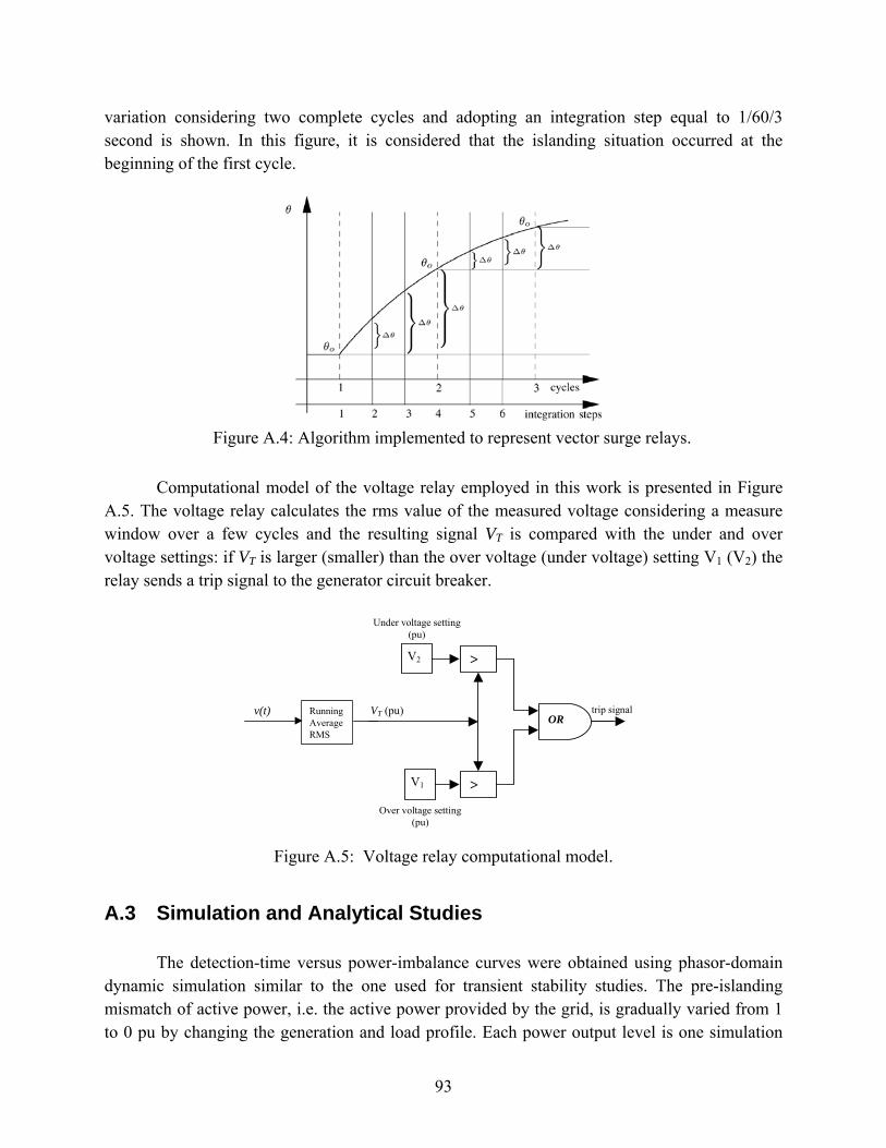
93

variation considering two complete cycles and adopting an integration step equal to 1/60/3 second is shown. In this figure, it is considered that the islanding situation occurred at the beginning of the first cycle.

Figure A.4: Algorithm implemented to represent vector surge relays.

Computational model of the voltage relay employed in this work is presented in Figure A.5. The voltage relay calculates the rms value of the measured voltage considering a measure window over a few cycles and the resulting signal VT is compared with the under and over voltage settings: if VT is larger (smaller) than the over voltage (under voltage) setting V1 (V2) the relay sends a trip signal to the generator circuit breaker.

Over voltage setting(pu)

trip signal

V2 >

V1 >

OR

Under voltage setting(pu)

VT (pu)RunningAverage RMS

v(t)

Figure A.5: Voltage relay computational model.

A.3 Simulation and Analytical Studies

The detection-time versus power-imbalance curves were obtained using phasor-domain dynamic simulation similar to the one used for transient stability studies. The pre-islanding mismatch of active power, i.e. the active power provided by the grid, is gradually varied from 1 to 0 pu by changing the generation and load profile. Each power output level is one simulation

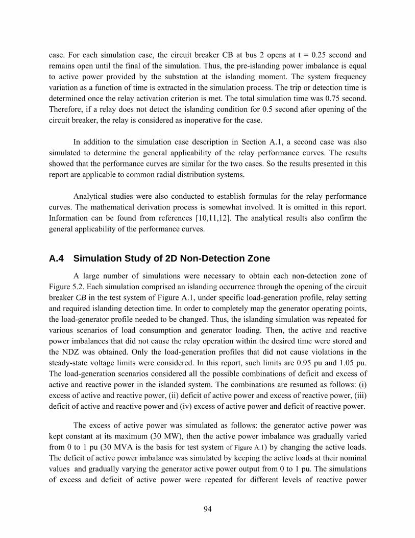
94

case. For each simulation case, the circuit breaker CB at bus 2 opens at t = 0.25 second and remains open until the final of the simulation. Thus, the pre-islanding power imbalance is equal to active power provided by the substation at the islanding moment. The system frequency variation as a function of time is extracted in the simulation process. The trip or detection time is determined once the relay activation criterion is met. The total simulation time was 0.75 second. Therefore, if a relay does not detect the islanding condition for 0.5 second after opening of the circuit breaker, the relay is considered as inoperative for the case. In addition to the simulation case description in Section A.1, a second case was also simulated to determine the general applicability of the relay performance curves. The results showed that the performance curves are similar for the two cases. So the results presented in this report are applicable to common radial distribution systems. Analytical studies were also conducted to establish formulas for the relay performance curves. The mathematical derivation process is somewhat involved. It is omitted in this report. Information can be found from references [10,11,12]. The analytical results also confirm the general applicability of the performance curves.

A.4 Simulation Study of 2D Non-Detection Zone

A large number of simulations were necessary to obtain each non-detection zone of Figure 5.2. Each simulation comprised an islanding occurrence through the opening of the circuit breaker CB in the test system of Figure A.1, under specific load-generation profile, relay setting and required islanding detection time. In order to completely map the generator operating points, the load-generator profile needed to be changed. Thus, the islanding simulation was repeated for various scenarios of load consumption and generator loading. Then, the active and reactive power imbalances that did not cause the relay operation within the desired time were stored and the NDZ was obtained. Only the load-generation profiles that did not cause violations in the steady-state voltage limits were considered. In this report, such limits are 0.95 pu and 1.05 pu. The load-generation scenarios considered all the possible combinations of deficit and excess of active and reactive power in the islanded system. The combinations are resumed as follows: (i) excess of active and reactive power, (ii) deficit of active power and excess of reactive power, (iii) deficit of active and reactive power and (iv) excess of active power and deficit of reactive power.

The excess of active power was simulated as follows: the generator active power was kept constant at its maximum (30 MW), then the active power imbalance was gradually varied from 0 to 1 pu (30 MVA is the basis for test system of Figure A.1) by changing the active loads. The deficit of active power imbalance was simulated by keeping the active loads at their nominal values and gradually varying the generator active power output from 0 to 1 pu. The simulations of excess and deficit of active power were repeated for different levels of reactive power

95

imbalances. The range of reactive power imbalance values comprised cases of deficit and excess of reactive power in the islanded system. In the case of AVR controlling terminal voltage, the AVR set point was varied from 0.95 pu to 1.05 pu. This guaranteed that there were cases of deficit and excess of reactive power. For each AVR set point, a simulation of deficit of active power and another of excess of active power were performed.

To obtain the NDZ considering Q control mode, the active power imbalance variation was performed as described previously. The reactive power imbalance variation was obtained as follows: the excess of reactive power was obtained by keeping the reactive loads constant at their nominal values and varying the generator reactive power output from a level equal to the loads consumption until the generator maximum capacity (18 MVAr for test system of Figure A.1). On the other side, the deficit of reactive power was simulated by keeping the reactive loads constant at their rated values and varying the generator reactive power output from 0 (zero) until the islanded loads rated reactive consumption (11 MVAr).

96

APPENDIX B. DETERMINATION OF NON-DETECTION ZONES

The non-detection zones of relays are represented as lookup tables for risk assessment. This Appendix discusses the methods to construct the lookup tables and the associated practical issues. As shown in Section 4.2.3, the characteristics of frequency-based relays can be modeled analytically. It is, therefore, possible to determine the NDZs of such relays using analytical equations. The characteristics of frequency relays can be described as:

)(2)(2

00 τφ

τφ

−=

−=Δ

dd tfHtfHP

(17)

where td is the detection time; τ is the time used to compute the frequency value and run the relay algorithm.

From manufacturers catalogs this intrinsic delay is around 80 ms, which is adopted here. H is the generator H constant; fo is the power system frequency; φ is the relay setting, for example 0.5Hz; and ΔP is the power mismatch between load and generation in absolute per-unit value defined as ΔP=|(Pgen-Pload)/Pgen-rated |

The characteristics of ROCOF relay are:

⎟⎟

⎠

⎞

⎜⎜

⎝

⎛−

=

⎟⎟

⎠

⎞

⎜⎜

⎝

⎛−

=Δ−−

a

d

a

d

Tt

oT

t

o efHef

HPττ

ββ

121

2

(18)

where β is the relay setting, for example, 1.2Hz/s; τ is the time used to compute the df/dt value and run the relay algorithm. If 3 From manufacturers catalogs this intrinsic delay is around 130 ms, which is adopted here. Ta is the time constant of a low pass filter that models the averaging algorithm to estimate df/dt. Typical value of Ta is 100 ms (or 6 cycles);

Although analytical formulas can be used to determine the performance of frequency-based relays, no analytical formulas are available to determine the performance of voltage relays. Therefore, solution through computer simulation is needed. In this case, a typical simple distribution system can be used to build the look-up table. In this project, we have used the test system shown in Figure B.1. In this figure, PL and QL are fictitious local active and reactive loads, PG and QG are the active and reactive power generated by the synchronous DG. VSUB is a voltage source representing a substation and ZLINE is an impedance representing a line. In

97

addition, in order to obtain the NDZ, the islanding situation is simulated by opening circuit breaker CB in Figure B.1. This fictitious system can be used to determine the NDZ of frequency-based and voltage relays as follows through a few simulations.

SG

RELAY

PL QL PG , QG

CB

ZLINE

VSUB

Figure B.1: Test system.

The determination of ΔP1, ΔP2, ΔQ1 and ΔQ2 can be done as follows: these points can be calculated through a few islanding simulations by using the system shown in Figure B.1 as follows:

• Set PG and QG

• ΔP1 calculation

(a) Do PL = PG and QL = QG (i.e. ΔP = ΔQ = 0) (b) Do PL = PL − ΔPL (i.e. decrease gradually the active load PL) (c) Simulate an islanding by opening the circuit breaker CB (d) If the islanding is detected by the protection system, go to (e). If not, go

to (b) (e) Do ΔP1 equal the last ΔP, which is calculated by PG − PL

• ΔP2 calculation

(a) Do PL = PG and QL = QG (i.e. ΔP = ΔQ = 0) (b) Do PL = PL + ΔPL (i.e. increase gradually the active load PL) (c) Simulate an islanding by opening the circuit breaker CB (d) If the islanding is detected by the protection system, go to (e). If not, go

to (b) (e) Do ΔP2 equal the last ΔP, which is calculated by PG − PL

• ΔQ1 calculation

(a) Do PL = PG and QL = QG (i.e. ΔP = ΔQ = 0)

98

(b) Do QL = QL − ΔQL (i.e. decrease gradually the reactive load QL8)

(c) Simulate an islanding by opening the circuit breaker CB (d) If the islanding is detected by the protection system, go to (e). If not, go

to (b) (e) Do ΔQ1 equal the last ΔQ, which is calculated by QG − QL

• ΔQ2 calculation

(a) Do PL = PG and QL = QG (i.e. ΔP = ΔQ = 0) (b) Do QL = QL + ΔQL (i.e. increase gradually the reactive load QL) (c) Simulate an islanding by opening the circuit breaker CB (d) If the islanding is detected by the protection system, go to (e). If not, go

to (b) (e) Do ΔQ2 equal the last ΔQ, which is calculated by QG − QL

Tables B.1. and B.2 show the lookup table values obtained by using repeated dynamic simulations and formulas (17) and (18), where one can see very good match among the formula and the simulation results. The table related to the voltage relay was presented in Chapter 7 (Table 7.3).

It is noted that the look-up table was determined using a specific test system. However, our extensive studies on other systems show that the errors of applying these tables to other typical distribution systems are acceptable. Indeed, the results related to the frequency-based relays are almost system independent, as can be confirmed by the usage of the analytical formulas since, in these formulas, no system parameters are necessary and the results are very accurate. On the other hand, the results related to the voltage relays change a little from system to system since the pre-islanding nodal voltage has some influence on the relay performance. For example, consider the following two distinct situations:

Case (a): the nodal voltage of the bus where the voltage relay is installed is 1.0 pu before the islanding and the islanding is detected by the under voltage settings;

Case (b): the nodal voltage of the bus where the voltage relay is installed is 0.95 pu before the islanding and the islanding is detected by the under voltage settings;

Obviously, the islanding situation will be detected a little bit faster in case (b) since the pre-islanding voltage is lower, consequently closer to the relay setting. However, the difference is small and as the nodal voltages of distribution system are typically regulated between 0.95 and 1.05 pu (or in a smaller range), the variation of the pre-islanding nodal voltage is small. Thus, the error resulting is also acceptable.

8 If QG is equal to zero, the load variation should be capacitive in order to have excess of reactive power.

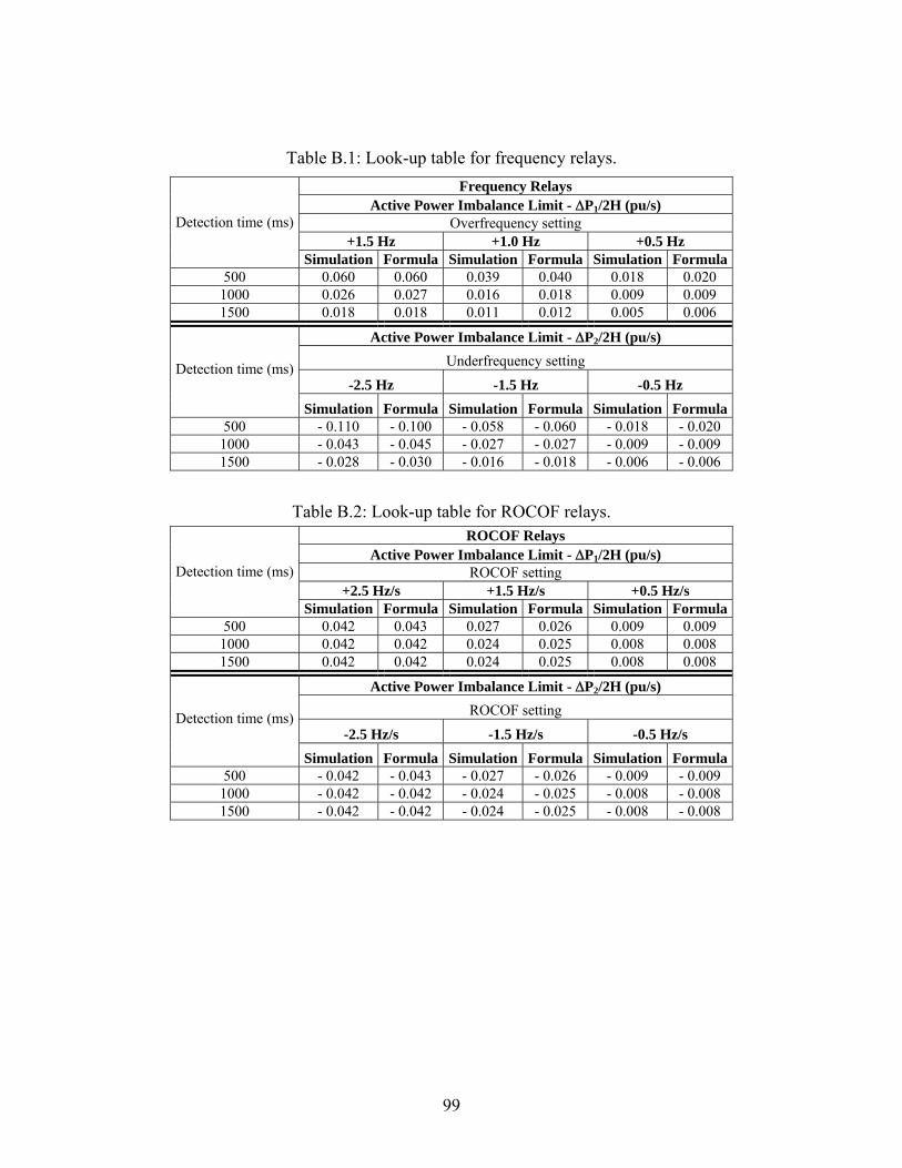
99

Table B.1: Look-up table for frequency relays. Frequency Relays

Active Power Imbalance Limit - ΔP1/2H (pu/s) Overfrequency setting

+1.5 Hz +1.0 Hz +0.5 Hz Detection time (ms)

Simulation Formula Simulation Formula Simulation Formula500 0.060 0.060 0.039 0.040 0.018 0.020

1000 0.026 0.027 0.016 0.018 0.009 0.009 1500 0.018 0.018 0.011 0.012 0.005 0.006

Active Power Imbalance Limit - ΔP2/2H (pu/s) Underfrequency setting

-2.5 Hz -1.5 Hz -0.5 Hz Detection time (ms)

Simulation Formula Simulation Formula Simulation Formula500 - 0.110 - 0.100 - 0.058 - 0.060 - 0.018 - 0.020

1000 - 0.043 - 0.045 - 0.027 - 0.027 - 0.009 - 0.009 1500 - 0.028 - 0.030 - 0.016 - 0.018 - 0.006 - 0.006

Table B.2: Look-up table for ROCOF relays. ROCOF Relays

Active Power Imbalance Limit - ΔP1/2H (pu/s) ROCOF setting

+2.5 Hz/s +1.5 Hz/s +0.5 Hz/s Detection time (ms)

Simulation Formula Simulation Formula Simulation Formula500 0.042 0.043 0.027 0.026 0.009 0.009

1000 0.042 0.042 0.024 0.025 0.008 0.008 1500 0.042 0.042 0.024 0.025 0.008 0.008

Active Power Imbalance Limit - ΔP2/2H (pu/s) ROCOF setting

-2.5 Hz/s -1.5 Hz/s -0.5 Hz/s Detection time (ms)

Simulation Formula Simulation Formula Simulation Formula500 - 0.042 - 0.043 - 0.027 - 0.026 - 0.009 - 0.009

1000 - 0.042 - 0.042 - 0.024 - 0.025 - 0.008 - 0.008 1500 - 0.042 - 0.042 - 0.024 - 0.025 - 0.008 - 0.008

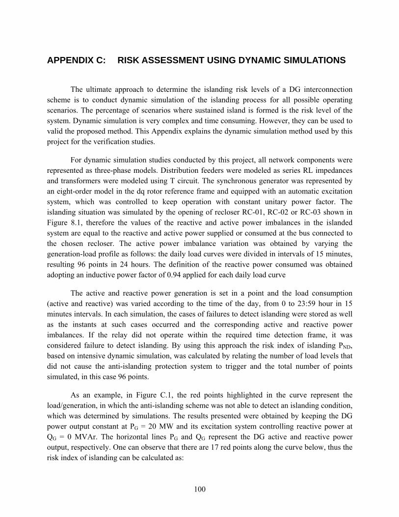
100

APPENDIX C: RISK ASSESSMENT USING DYNAMIC SIMULATIONS

The ultimate approach to determine the islanding risk levels of a DG interconnection scheme is to conduct dynamic simulation of the islanding process for all possible operating scenarios. The percentage of scenarios where sustained island is formed is the risk level of the system. Dynamic simulation is very complex and time consuming. However, they can be used to valid the proposed method. This Appendix explains the dynamic simulation method used by this project for the verification studies.

For dynamic simulation studies conducted by this project, all network components were represented as three-phase models. Distribution feeders were modeled as series RL impedances and transformers were modeled using T circuit. The synchronous generator was represented by an eight-order model in the dq rotor reference frame and equipped with an automatic excitation system, which was controlled to keep operation with constant unitary power factor. The islanding situation was simulated by the opening of recloser RC-01, RC-02 or RC-03 shown in Figure 8.1, therefore the values of the reactive and active power imbalances in the islanded system are equal to the reactive and active power supplied or consumed at the bus connected to the chosen recloser. The active power imbalance variation was obtained by varying the generation-load profile as follows: the daily load curves were divided in intervals of 15 minutes, resulting 96 points in 24 hours. The definition of the reactive power consumed was obtained adopting an inductive power factor of 0.94 applied for each daily load curve

The active and reactive power generation is set in a point and the load consumption (active and reactive) was varied according to the time of the day, from 0 to 23:59 hour in 15 minutes intervals. In each simulation, the cases of failures to detect islanding were stored as well as the instants at such cases occurred and the corresponding active and reactive power imbalances. If the relay did not operate within the required time detection frame, it was considered failure to detect islanding. By using this approach the risk index of islanding PND, based on intensive dynamic simulation, was calculated by relating the number of load levels that did not cause the anti-islanding protection system to trigger and the total number of points simulated, in this case 96 points.

As an example, in Figure C.1, the red points highlighted in the curve represent the load/generation, in which the anti-islanding scheme was not able to detect an islanding condition, which was determined by simulations. The results presented were obtained by keeping the DG power output constant at PG = 20 MW and its excitation system controlling reactive power at QG = 0 MVAr. The horizontal lines PG and QG represent the DG active and reactive power output, respectively. One can observe that there are 17 red points along the curve below, thus the risk index of islanding can be calculated as:

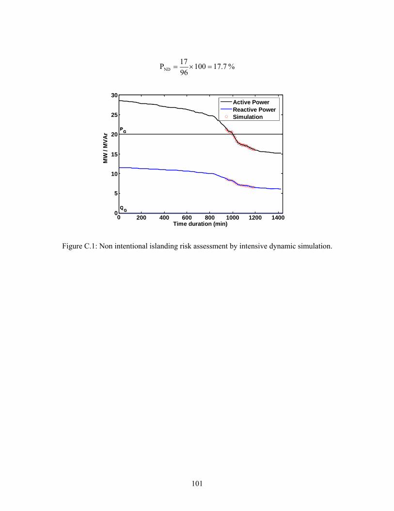
101

% 17.71009617PND =×=

0 200 400 600 800 1000 1200 14000

5

10

15

20

25

30

Time duration (min)

MW

/ M

VAr

P G

Q G

P G

Q G

Active PowerReactive PowerSimulation

Figure C.1: Non intentional islanding risk assessment by intensive dynamic simulation.

102

APPENDIX D: RISK ASSESSMENT FOR SYSTEMS WITH CONSTANT IMPEDANCE LOADS

From Figure D.1, one can see that the characteristic of the load has great influence on the NDZ shape and limits. Indeed, the NDZs in the presence of constant impedance loads, which are voltage-dependent loads, are usually larger and have an irregular shape. We use this Appendix to explain how to use the lookup tables to deal with the situation.

-1 -0.8 -0.6 -0.4 -0.2 0 0.2 0.4 0.6 0.8 1-1 -0.8 -0.6 -0.4 -0.2

0 0.2 0.4 0.6 0.8

1

Active power imbalance (pu)

Rea

ctiv

e po

wer

imba

lanc

e (p

u)

(a) constant power load.

-1 -0.8 -0.6 -0.4 -0.2 0 0.2 0.4 0.6 0.8 1-1

-0.8

-0.6

-0.4

-0.2

0

0.2

0.4

0.6

0.8

1

Active power imbalance (pu)

Rea

ctiv

e po

wer

imba

lanc

e (p

u)

(b) constant impedance load.

Figure D.1: Typical NDZ for different types of loads (relay settings: frequency relay: 57.5/61.5Hz; voltage relay: 0.5/1.2pu).

Based on results obtained from a large number of cases, it was verified that the NDZs in the presence of constant impedance loads is inclined with relation to the NDZ of constant power loads. The limits related to the active power imbalances (i.e., ΔP1 and ΔP2) do not change considerably. The limits related to the reactive power imbalances (i.e., ΔQ1 and ΔQ2) change considerably. With these observations, the following procedure is proposed to calculate the NDZ in the presence of constant impedance loads:

• The rectangular NDZ for constant power loads is determined first. Based on the result, new reactive imbalance limits ΔQ’1 and ΔQ’2 are calculated by increasing ΔQ1

by 20 % and ΔQ2 by 120 %, respectively. Therefore, we have a four straight lines NDZ but with new limits (0,ΔQ’1) and (0,ΔQ’2) as shown in Figure D.2(a).

• The newly modified NDZ is then rotated by a certain angle. The rotation angle of 30 degrees was determined empirically through observations of several simulations. This last step is shown graphically in Figure D.2(b).

103

Δ P

Δ Q

ΔP1 ΔP2

ΔQ1

ΔQ2

ΔQ’1

ΔQ’2

original NDZ

modified NDZ

(a)

Δ P

Δ Q

ΔP1 ΔP2

ΔQ’1

ΔQ’2

30 degrees NDZ in the presence of constant impedance loads

(b)

Figure D.2: NDZ for constant impedance load.

The above procedure to estimate the NDZ in the presence of constant impedance loads is validated in Figure D.3, where the non-detection zones calculated by the proposed method is compared with the those obtained by intensive dynamic simulations. The test system presented in Figure 8.1 was used in this study. From this figure, one can see that the proposed method presents good accuracy.

104

-1 -0.8 -0.6 -0.4 -0.2 0 0.2 0.4 0.6 0.8 1-1 -0.8 -0.6 -0.4 -0.2

0 0.2 0.4 0.6 0.8

1

Active power imbalance (pu)

Rea

ctiv

e po

wer

imba

lanc

e (p

u) Intensive Simulation

Proposed Method

(a) Frequency and voltage relays 57.5/61.5 Hz – 0.5/1.2 pu.

-1 -0.8 -0.6 -0.4 -0.2 0 0.2 0.4 0.6 0.8 1-1

-0.8

-0.6

-0.4

-0.2

0

0.2

0.4

0.6

0.8

1

Active power imbalance (pu)

Rea

ctiv

e po

wer

imba

lanc

e (p

u) Intensive Simulation

Proposed Method

(c) ROCOF and voltage relays 2.5 Hz/s – 0.5/1.2 pu.

-1 -0.8 -0.6 -0.4 -0.2 0 0.2 0.4 0.6 0.8 1-1 -0.8 -0.6 -0.4 -0.2

0 0.2 0.4 0.6 0.8

1

Active power imbalance (pu)

Rea

ctiv

e po

wer

imba

lanc

e (p

u) Intensive Simulation

Proposed Methodology

(b Frequency and voltage relays 59.5/61.0 Hz – 0.5/1.2 pu.

-1 -0.8 -0.6 -0.4 -0.2 0 0.2 0.4 0.6 0.8 1-1

-0.8

-0.6

-0.4

-0.2

0

0.2

0.4

0.6

0.8

1

Active power imbalance (pu)

Rea

ctiv

e po

wer

imba

lanc

e (p

u)

(d) ROCOF and voltage relays 0.5 Hz/s – 0.5/1.2 pu

Figure D.3: Non-detection zones determined from the look-up tables and from intensive dynamic simulations in the presence of constant impedance loads (required detection time = 500 ms)

In order to calculate the risk index in the presence of constant impedance load, it is necessary to apply an axis rotation to the PQ axis since the proposed method is based on the usage of constant active and reactive power bands around the generator power in the plane power versus time. This method is summarized in the following steps.

• A new PQ axis of the NDZ is calculated by rotating them shown in Figure D.4. The ΔP-axis and ΔQ-axis are rotated so that the NDZ associated to constant impedance is made parallel to these two axes. Since the NDZ associated to constant impedance load is obtained by rotating clockwise the NDZ associated to constant power loads by 30 degrees with respect to ΔQ-axis, thus the original reference ΔQ x ΔP should also be rotated so that the new ΔQnew-axis is 30 degrees advanced in the clockwise direction with respect the original ΔQ-axis reference. The new axis system is shown in Figure D.4, where the new reference (ΔQnew x ΔPnew) is placed. Mathematically, this transformation is done as follows:

)()cos( θθ QsinPPnew −= (19)

105

)cos()( θθ QPsinQnew += (20)

where θ is the angle between ΔQnew and ΔQ original, measured in clockwise direction, which was adopted equal to 30 degrees based on many simulations.

• The active and reactive power injected by the distributed generator and the daily active and reactive power load curves must also be transformed to the new reference (ΔPnew x ΔQnew) by using (19) and (20).

Δ P

Δ Q

ΔP1

ΔP2

ΔQ’2

30 degrees

ΔQnew ΔQ’1

ΔPnew

ΔP2new

ΔP1new

ΔQ1new

ΔQ2new

Figure D.4: Axis rotation.

• The case now becomes one that resembles the constant power load case. The difference is that new ΔP and ΔQ values are used. The procedure described in Chapter 7 can now be used to determine the risk indices. It is important to note, however, that the PQ axis transformation must also be applied to the active and reactive powers of load and generation.

106

APPENDIX E: EXAMPLE OF TIME DOMAIN SIMULATION RESULTS

In this appendix, some examples of time domain results are presented. The results were obtained by using the system of Fig. 8.1 and a program of electromagnetic transient simulations. In all cases presented here, the islanding situation was simulated by opening recloser RC-01 at t = 0.25 second. Two loading/generation cases are presented as follows:

Case 1:

• The active power supplied by the generator was set equal to 20 MW.

• The total system active and reactive loads were set equal to 25 MW and 8.53 MVAr, respectively.

Case 2:

• The active power supplied by the generator is set equal to 20 MW.

• The total system active and reactive loads are set equal to 18 MW and 6.41 MVAr, respectively.

In addition, for each case, there are four distinct situations as follows:

Situation 1: The loads are represented by constant impedance models (ZC) and the generator excitation system is controlled to maintain constant terminal voltage at 1 pu (VC). In the following figures, this situation is denoted by ZC / VC in the legends.

Situation 2: The loads are represented by constant impedance models (ZC) and the generator excitation system is controlled to maintain constant reactive power at 0 MVAr (QC). In the following figures, this situation is denoted by ZC / QC in the legends.

Situation 3: The loads are represented by constant power models (PC) and the generator excitation system is controlled to maintain constant terminal voltage at 1 pu (VC). In the following figures, this situation is denoted by PC / VC in the legends.

Situation 4: The loads are represented by constant power models (PC) and the generator excitation system is controlled to maintain constant reactive power at 0 MVAr (QC). In the following figures, this situation is denoted by PC / QC in the legends.

107

E.1. Simulation Results

The behavior of the main system variables for Cases 1 and 2 and considering the four distinct situations is presented in Figures E.1 and E.2, respectively. From these figures, one can see that the type of load and the type of excitation system control mode have great influence on the system variables' behavior.

In Fig. E.1(a), one can see that the generator terminal voltage collapses when the excitation system is set to reactive power control mode, since there is deficit of reactive power in the islanding system, as shown in Fig. E.1(d). On the other hand, when the excitation system is set to voltage control mode, the terminal voltage recovers to 1 pu after the islanding.

In Fig. E.1(b), for three situations, the frequency decreases after islanding since there is deficit of active power in the islanding system, as shown in Fig. E.1(c). However, in the case with constant impedance loads and reactive power excitation control mode, the frequency increases since, in this situation, there is excess of active power after the islanding, as shown in Fig. E.1(c). This occurs because the total load demand decreases after the islanding as a consequence of the nodal voltage reduction, as can be seen in Fig. E.1(g) for bus 8 load.

It is worth highlighting that, for these examples, in the situations where the loads are represented by constant power models and the generator excitation system controls reactive power, the simulation is aborted at t = 0.625 second, for Case 1, and at t = 0.935 second, for Case 2, because, at this point, the generator terminal voltage is lower than 0.2 pu and, consequently, some numerical convergence problem can arise. However, this is not a problem for most cases presented in this report since the simulation time after islanding is limited to 0.5 second in addition, the instantaneous setting for the voltage relay is higher than 0.2 pu.

108

0 0.5 1 1.5 20

0.2

0.4

0.6

0.8

1

1.2

Case 1

Time (s)

Gen

erat

or te

rmin

al v

olta

ge (p

u)

Zc / VcZc / QcPc / VcPc / Qc

(a) generator terminal voltage

0 0.5 1 1.5 250

55

60

65

70

75Case 1

Time (s)

Freq

uenc

y (H

z)

Zc / VcZc / QcPc / VcPc / Qc

(b) system frequency

0 0.5 1 1.5 2-0.5

-0.4

-0.3

-0.2

-0.1

0

0.1

0.2

0.3

0.4

0.5Case 1

Time (s)

Act

ive

pow

er u

nbal

ance

(pu)

Zc / VcZc / QcPc / VcPc / Qc

(c) active power unbalance

0 0.5 1 1.5 2-0.5

-0.4

-0.3

-0.2

-0.1

0

0.1

0.2

0.3

0.4

0.5Case 1

Time (s)

Rea

ctiv

e po

wer

unb

alan

ce (p

u)

Zc / VcZc / QcPc / VcPc / Qc

(d) reactive power unbalance

0 0.5 1 1.5 20

0.5

1

1.5Case 1

Time (s)

Gen

erat

or a

ctiv

e po

wer

(pu)

Zc / VcZc / QcPc / VcPc / Qc

(e) generator active power

0 0.5 1 1.5 2-0.2

0

0.2

0.4

0.6

0.8

Case 1

Time (s)

Gen

erat

or re

activ

e po

wer

(pu)

Zc / VcZc / QcPc / VcPc / Qc

(f) generator reactive power

0 0.5 1 1.5 20

0.5

1

1.5

2

2.5

3

3.5

4 x 106 Case 1

Time (s)

Bus

8 a

ctiv

e po

wer

load

(pu)

Zc / VcZc / QcPc / VcPc / Qc

(g) bus 8 active power load

0 0.5 1 1.5 20

5

10

15 x 105 Case 1

Time (s)

Bus

8 a

ctiv

e po

wer

load

(pu)

Zc / VcZc / QcPc / VcPc / Qc

(h) bus 8 reactive power load

Figure E.1: Time domain response for case 1.

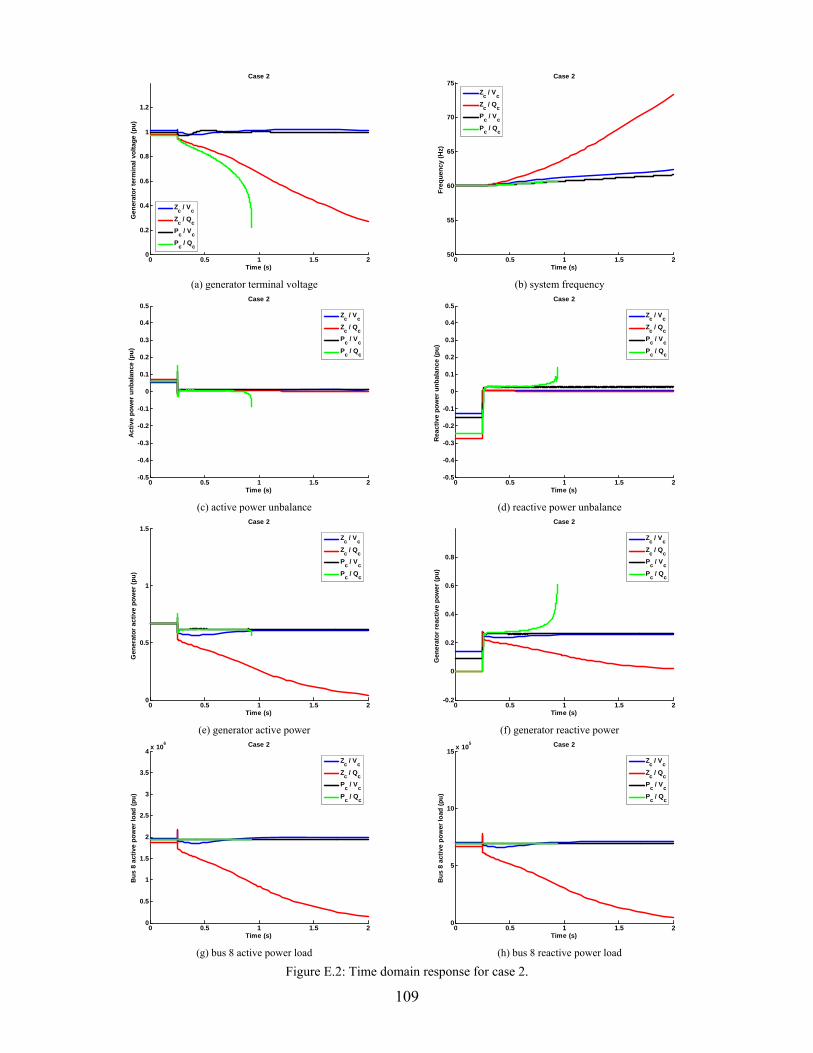
109

0 0.5 1 1.5 20

0.2

0.4

0.6

0.8

1

1.2

Case 2

Time (s)

Gen

erat

or te

rmin

al v

olta

ge (p

u)

Zc / VcZc / QcPc / VcPc / Qc

(a) generator terminal voltage

0 0.5 1 1.5 250

55

60

65

70

75Case 2

Time (s)

Freq

uenc

y (H

z)

Zc / VcZc / QcPc / VcPc / Qc

(b) system frequency

0 0.5 1 1.5 2-0.5

-0.4

-0.3

-0.2

-0.1

0

0.1

0.2

0.3

0.4

0.5Case 2

Time (s)

Act

ive

pow

er u

nbal

ance

(pu)

Zc / VcZc / QcPc / VcPc / Qc

(c) active power unbalance

0 0.5 1 1.5 2-0.5

-0.4

-0.3

-0.2

-0.1

0

0.1

0.2

0.3

0.4

0.5Case 2

Time (s)

Rea

ctiv

e po

wer

unb

alan

ce (p

u)

Zc / VcZc / QcPc / VcPc / Qc

(d) reactive power unbalance

0 0.5 1 1.5 20

0.5

1

1.5Case 2

Time (s)

Gen

erat

or a

ctiv

e po

wer

(pu)

Zc / VcZc / QcPc / VcPc / Qc

(e) generator active power

0 0.5 1 1.5 2-0.2

0

0.2

0.4

0.6

0.8

Case 2

Time (s)

Gen

erat

or re

activ

e po

wer

(pu)

Zc / VcZc / QcPc / VcPc / Qc

(f) generator reactive power

0 0.5 1 1.5 20

0.5

1

1.5

2

2.5

3

3.5

4 x 106 Case 2

Time (s)

Bus

8 a

ctiv

e po

wer

load

(pu)

Zc / VcZc / QcPc / VcPc / Qc

(g) bus 8 active power load

0 0.5 1 1.5 20

5

10

15 x 105 Case 2

Time (s)

Bus

8 a

ctiv

e po

wer

load

(pu)

Zc / VcZc / QcPc / VcPc / Qc

(h) bus 8 reactive power load

Figure E.2: Time domain response for case 2.