project thesis token-based compression -...

Project Thesis

Token-Based Compression

van Beusekom Joost

May 18, 2005

Contents

1 Introduction 5

1.1 Token-Based Compression . . . . . . . . . . . . . . . . . . . . . . 51.2 Use of Token-Based Compression . . . . . . . . . . . . . . . . . . 61.3 Overview . . . . . . . . . . . . . . . . . . . . . . . . . . . . . . . 6

1.3.1 Goal . . . . . . . . . . . . . . . . . . . . . . . . . . . . . . 61.3.2 Processing Steps . . . . . . . . . . . . . . . . . . . . . . . 6

2 Main Part 9

2.1 Binarization . . . . . . . . . . . . . . . . . . . . . . . . . . . . . . 92.1.1 General Description . . . . . . . . . . . . . . . . . . . . . 92.1.2 Global Thresholding . . . . . . . . . . . . . . . . . . . . . 92.1.3 Local Adaptive Thresholding . . . . . . . . . . . . . . . . 112.1.4 Difference image . . . . . . . . . . . . . . . . . . . . . . . 122.1.5 Results . . . . . . . . . . . . . . . . . . . . . . . . . . . . 13

2.2 Connected Components . . . . . . . . . . . . . . . . . . . . . . . 142.2.1 General Description . . . . . . . . . . . . . . . . . . . . . 142.2.2 Region Growing . . . . . . . . . . . . . . . . . . . . . . . 152.2.3 Labelling . . . . . . . . . . . . . . . . . . . . . . . . . . . 152.2.4 Results . . . . . . . . . . . . . . . . . . . . . . . . . . . . 182.2.5 Creation of the Residual Image . . . . . . . . . . . . . . . 18

2.3 Noise Removal . . . . . . . . . . . . . . . . . . . . . . . . . . . . 182.3.1 General Description . . . . . . . . . . . . . . . . . . . . . 182.3.2 Results . . . . . . . . . . . . . . . . . . . . . . . . . . . . 19

2.4 Similarity Measurement . . . . . . . . . . . . . . . . . . . . . . . 192.4.1 General Description . . . . . . . . . . . . . . . . . . . . . 192.4.2 Similarities . . . . . . . . . . . . . . . . . . . . . . . . . . 202.4.3 Lossy/Lossless Compression . . . . . . . . . . . . . . . . . 282.4.4 Compression of multiple pages with one dictionary . . . . 292.4.5 Implementation Details . . . . . . . . . . . . . . . . . . . 31

2.5 Reconstruction . . . . . . . . . . . . . . . . . . . . . . . . . . . . 332.5.1 General Description . . . . . . . . . . . . . . . . . . . . . 332.5.2 Composition of the substitutions . . . . . . . . . . . . . . 342.5.3 Lossless compression . . . . . . . . . . . . . . . . . . . . . 34

3 Results 36

3.1 Lossy Compression with new dictionaries . . . . . . . . . . . . . 363.2 Lossless Compression with new dictionaries . . . . . . . . . . . . 373.3 Lossy Compression with re-used dictionary . . . . . . . . . . . . 38

1

3.4 Lossless Compression with re-used dictionary . . . . . . . . . . . 39

4 Conclusion & Open Problems 41

2

List of Figures

2.1 Greyscale values, black is value 0, white value 255 . . . . . . . . 92.2 Example of global thresholding . . . . . . . . . . . . . . . . . . . 102.3 Example of adaptive thresholding . . . . . . . . . . . . . . . . . . 122.4 Example of histograms generated with GIMP . . . . . . . . . . . 122.5 Example of difference method for binarization . . . . . . . . . . . 142.6 Example of connected components with their bounding boxes . . 152.7 Example for the labelling method for extracting connected com-

ponents . . . . . . . . . . . . . . . . . . . . . . . . . . . . . . . . 172.8 Example of a residual image of image 2.2(a) . . . . . . . . . . . . 182.9 Example of 4 classes of tokens. The first token in each row is the

prototype . . . . . . . . . . . . . . . . . . . . . . . . . . . . . . . 202.10 Example for pixelwise comparison . . . . . . . . . . . . . . . . . 212.11 Example for problem with naive pixel difference method . . . . . 222.12 Example for superimposing two tokens . . . . . . . . . . . . . . . 242.13 An example for a turtle looking in direction 0 (a), and one for

looking in direction 1 (b) . . . . . . . . . . . . . . . . . . . . . . 252.14 Example for the three different pixels that need to be checked for

the Pavlidis algorithm . . . . . . . . . . . . . . . . . . . . . . . . 262.15 Example for the Pavlidis algorithm for extracting the contour of

a token . . . . . . . . . . . . . . . . . . . . . . . . . . . . . . . . 272.16 Example for updating the residual image . . . . . . . . . . . . . . 302.17 Example of a part of a residual image . . . . . . . . . . . . . . . 302.18 Example for the format of a prototype image . . . . . . . . . . . 312.19 Example for prototype image . . . . . . . . . . . . . . . . . . . . 312.20 Example for the use of the substitutions information . . . . . . . 32

3

List of Tables

2.1 Example for the entries in the substitutions data file . . . . . . . 34

3.1 Size of resulting ZIP-file compared to the size of different otherimage formats for lossy compression with new dictionaries . . . . 36

3.2 Performance of the proposed method for lossy compression withnew dictionaries . . . . . . . . . . . . . . . . . . . . . . . . . . . . 36

3.3 Space needed for the different resulting files. . . . . . . . . . . . . 363.4 Size of resulting ZIP-file compared to the size of different other

image formats for lossless compression with new dictionaries . . . 373.5 Performance of the proposed method for lossless compression

with new dictionaries . . . . . . . . . . . . . . . . . . . . . . . . . 373.6 Space needed for the different resulting files. . . . . . . . . . . . . 373.7 Size of resulting ZIP-file compared to the size of different other

image formats for lossy compression with re-used dictionaries . . 383.8 Performance of the proposed method for lossy compression with

re-used dictionaries . . . . . . . . . . . . . . . . . . . . . . . . . . 393.9 Space needed for the different resulting files. . . . . . . . . . . . . 393.10 Size of resulting ZIP-file compared to the size of different other

image formats for lossless compression with re-used dictionaries . 393.11 Performance of the proposed method for lossless compression

with re-used dictionaries . . . . . . . . . . . . . . . . . . . . . . . 403.12 Space needed for the different resulting files. . . . . . . . . . . . . 40

4

Chapter 1

Introduction

1.1 Token-Based Compression

Token-Based Compression (TBC) was first introduced by Ascher and Nagy[AN74]. The basic idea was to speed up digital transmission of scanned docu-ments, by sending only the “new” tokens (here a token can be seen as a scannedcharacter), where “new” means that this kind of token has not been sent before.If a new, unknown token is to be sent, it is saved in a dictionary and then trans-mitted as image. The receiver gets the image and saves it in the dictionary andin the output image. If the token to be sent has already been transmitted thenonly the number of the token in the dictionary will be transmitted. The otherside then knows that is has to take the token saved previously in the dictionary.

The word ”Otto” for example would be transmitted in the following way(suppose we are reading from left to right): first the token “O” is read andtransmitted as image and saved into both dictionaries. The dictionaries nowcontain “1:image(O)”. Then for the first “t” the procedure is the same. Nowthe dictionaries contain “1:image(O), 2:image(t)”. For the second “t”, the pro-gram recognises that is has already a similar token in the dictionary of thesender, and thus only transmits the number of the token. In this case it wouldbe 2. The receiver now knows that he has to put the token 2 of his dictionaryto the specified location. The last character “o” is a new character, and it isprocessed as the first one.

The basic concept of this method can be found in an image format called”DjVu” [BHH+98]. This format uses a lot of techniques in order to achievebetter compression rates for black-and-white and colour documents. For bi-tone scanned documents (documents holding only black or white pixels) “DjVu”utilises a method called JB2. JB2 is a TBC-implementation for black-and-whitescanned documents. It is a variation of a the JBIG2 standard invented byAT&T’s for fax compression.

5

1.2 Use of Token-Based Compression

There are a lot of huge libraries and archives containing many documents, books,magazines, etc. In order to share these over the World Wide Web (or any otherdigital network), these books need to be digitised. After digitising, one imageof every single page is obtained. These images can be compressed by standardcompression techniques, but even then they are far too big to be downloaded ina reasonable amount of time. One way to decrease the space used by the image,is to use a lower resolution, which decreases the readability of the text. Theother way is to use Optical Character Recognition for converting the image intotext.

Despite all the progress that has been done in the domain of Optical Charac-ter Recognition (OCR), OCR still does not work accurate enough for digitisingin an unsupervised way, whole archives of scanned documents. The other prob-lem is that commercial OCR systems are very expensive.

So another way has to be gone in order to share whole libraries of documentsover the Internet. This can be done by Token-Based Compression, a compres-sion technique that has been developed especially for compressing scanned doc-uments. With this method it is possible (as shown by ”DjVu”) to share largeamounts of scanned documents, because of their very small file size, comparedwith other image formats.

1.3 Overview

1.3.1 Goal

The aim of this project thesis was to implement a TBC method to test howgood a simple approach to this technique would work. The program should alsoallow to compress lossless and lossy. Lossless compression means that the origi-nal image has to be reconstructed identically. For lossy compression, the imageshould contain the same information, but slight differences are allowed, as longas they don’t change the information it contains, e.g. changing a “c” to an “e”.Furthermore it should be possible to use one dictionary for more than one page(e.g. to use a dictionary for 30 pages scanned out of the same book). Here, inthis document, the word “dictionary” refers to a special image file containingthe prototypes of the tokens. A prototype is one token that has been chosen as“representative” of this class of tokens. To keep the introduction understand-able, a token will here be seen as an image of a character. Different tokens mayall contain the same character. These tokens should then be regarded as thesame class of tokens, or, in other words, they are considered “similar”.

1.3.2 Processing Steps

Binarization The first step is to binarize a greyscale image. Binarization isthe process of converting a greyscale image to a black-and-white image. Thiscan be done by a global threshold that sets a pixel to black if the value of thepixel is below the threshold, otherwise it is set to white. This method works

6

fast, but quite badly for images where the illumination is not uniform.

The method used here, is a local adaptive thresholding method. For a neigh-bouring region of the pixel, a local threshold is calculated, and the pixel is setto black or white, according to this local threshold.

An other method that has been implemented, first calculates the backgroundand foreground image by histogram manipulations. Then it compares the back-ground image with the foreground image to get the binarized image whichconsists ideally only of the characters. We called this method the “differencemethod”.

Connected Components The second step consists of extracting the con-nected components. A connected component is a set of black pixels that areconnected. “Connected” means, in this case, that the black pixels are ”touch-ing” each other.

This algorithm uses a wide-spread labelling method using a ”union-find”data structure. Region Growing has also been implemented.

In this part of the program, the residual image is created. This image con-tains all connected components that are larger than a certain amount of thetotal size of the page (e.g. 5%). These connected components are simply savedin the residual image. This image is later used for reconstruction of the originalimage.

Noise Reduction This part simply scans for connected components that con-tain only a very small number of black pixels (e.g. 4 or fewer). These connectedcomponents are simply considered as noise and are removed from further pro-cessing.

Token Recognition & Similarities This part of the process scans the con-nected components for tokens that are similar and then saves a dictionary con-taining only prototypes and a text file containing information about the posi-tions of the tokens, used for reconstruction. In the case of lossless compression,it also saves the pixels of the original token, that differ from the prototype inorder to allow a lossless reconstruction. This data is saved in the residual image.

The similarity between two tokens is calculated in two steps: the idea wasto try different methods of similarity measurement. Finally, it has been tried todo a first step that can be done quickly. Then afterwards pixelwise comparisonis done. One method that has been used for the first step used central momentsof the tokens.

The second method used Fast Fourier Transform (FFT): the idea is to con-sider the positions of the pixels of the contour of a token as a complex function.Then this function is Fourier transformed and the resulting Fourier coefficientsare used to compare two tokens. The Fourier coefficients contain informationabout the contour of the token. The first Fourier coefficients represent the low

7

frequencies of the contour, that means the rough contour. The last coefficientsrepresent the high frequencies (and the noise). So it is enough to compare onlythe first few coefficients and only if these are somehow similar, the second step,namely pixelwise comparison, is done.

If pixelwise comparison gives us two similar tokens, then only the position ofthe new token, and the number of the replacing prototype is saved. Otherwisea the new token is saved as prototype.

In order to allow the use of one dictionary for more than one page, theprogram allows to read a dictionary before proceeding with the image to becompressed.

Is also allows to update the residual image, created during the extraction ofthe connected components, in order to allow lossless compression.

Reconstruction This part of the project work does the reconstruction ofthe original image out of the dictionary (an image containing the prototypes),the positions data (information about where in the original image to put whatprototype) and the substitutions. The uses of the substitutions has becomenecessary because of the saving method for the prototypes: as these are sortedbefore saving them to the image file, their original unique number is lost. Soadditional information has to be saved to allow us to reconstruct the originalprototype number of each prototype. This original number is the number thatis saved in the positions data to give us the number of the prototype that isneeded in a certain location of the image.

8

Chapter 2

Main Part

2.1 Binarization

2.1.1 General Description

Binarization is the process that converts an greyscale image to a binary image(black-and-white image). In our case the greyscale values are 8bit values. “8bitgreyscale” means that each pixel is coded by 8 bits. This 8 bits give the darknessrespectively the lightness of the pixel. Value 0 is ”black”, value 128 is grey, value255 is white. See also figure 2.1. Ideally, binarization separates background(paper) from foreground (characters, text).

• Input: - a greyscale image

• Output: - a binarized (black-and-white) image

Figure 2.1: Greyscale values, black is value 0, white value 255

2.1.2 Global Thresholding

Binarization can be done by a global threshold. An example for global thresh-olding is given by the following algorithm:

01 INT threshold = 128 ; /*suppose 8bit greyscale images*/

02 FOR every pixel DO

03 IF (value of pixel >= threshold) THEN set pixel to white ;

04 ELSE set pixel to black ;

In other words: if a pixel is darker as our threshold, it is set to black. In theother case it is set to white. As shown in the figure 2.2, this method fails if theillumination of the scanned document is not uniform.

9

(a) Original greyscale image [Rei]

(b) Binarized with global threshold 128

(c) Binarized with global threshold 64

Figure 2.2: Example of global thresholding

10

2.1.3 Local Adaptive Thresholding

Basic Algorithm Instead of using one global threshold for all the pixels, localthresholding calculates a local threshold for every pixel. An example for thisadaptive thresholding is the following algorithm [Dav97]:

01 minrange = 255/5 ;

02 FOR each pixel DO

03 find minimum and maximum of local intensity distribution ;

04 range = maximum - minimum ;

05 IF range > minrange

06 THEN T := (minimum + maximum)/2 ;

07 ELSE T := maximum - minrange/2 ;

08 IF value of pixel > T

09 THEN thresholded pixel = 255 ; /*white*/

10 ELSE thresholded pixel = 0 ; /*black*/

11 END FOR ;

The idea behind this algorithm is the following: first determine a value“minrange” that gives us the least likely difference in intensity between a darkpixel (foreground, text) and a bright pixel (background, paper) in a window(i.e. 40x40 pixels).

Then every pixel is examined: first we get the maximum and minimum inintensity of the neighbouring pixels. The method we used to get the maximumand the minimum for this window is explained in the next paragraph. Then weget the difference between the maximum and the minimum.

If this difference (range) is greater than the minrange then we have the casethat we have some foreground and some background pixels in our window weexamined. Therefore we set our threshold T to the mean of the sum of themaximum and the minimum. This means that our pixel has to be darker thanthis mean in order to be identified as black pixel.

In case that our difference is smaller than the minrange we suppose that weonly have background pixels that only differ a little from each other. Thereforeour threshold is set to a lower value, namely maximum − minrange/2. Thisallows pixels to turn black that are relatively dark in comparison with theirsurroundings, e.g. if the background is quite dark.

The last step is simply comparing the value of our input (greyscale) pixelto the threshold we calculated for this pixel and its window, and setting thecorresponding output pixel to black or white.

Finding Minima and Maxima The first method used was to checka two-dimensional window with size l × l for minimum and maximum. Thismethod worked well but was very slow. For a picture of m × n pixels we getapproximately m × n × l2 passes of the inner loop.

We then tried to do this calculation only for a predefined grid. All the othervalues were interpolated linearly. This worked faster and the results were still

11

good.

The second method works in two steps: first it checks for each row in a one-dimensional window of size l for the maximum and the minimum and saves thesefor each pixel. Then in the second step, it checks for each column the maximumand minimum in a window of size l out of the maxima and minima found in thefirst step. So we get the maximum and minimum for a two-dimensional windowof size l × l but with less computational effort. For a picture of m × n we getm × l × n + n × l × m = 2 × l × n × m passes of the inner loop.

(a) Original greyscale image (b) Adaptively binarized, with window-size 40pix

Figure 2.3: Example of adaptive thresholding

2.1.4 Difference image

Another method that has been tried, is to calculate an approximate backgroundimage, an approximate foreground image and then to calculate the differenceimage.

This method uses histograms. A histogram of a greyscale image is nothingelse but a summary of how often what greyscale pixel (what value) appears.Figure 2.4(a) shows us the histogram of 2.2(a). As one can see, there is a lotof darker pixels and a peak with light grey pixels. Figure 2.4(b) shows us thehistogram of 2.1. As every value of pixel appears equally often, this histogramlooks like a constant function with the number of pixels of every greyscale valueas height.

(a) Histogram of 2.2(a) (b) Histogram of 2.1

Figure 2.4: Example of histograms generated with GIMP

12

The foreground 2.5(b) and background image 2.5(a) are calculated by a kindof histogram filter. For a window of size l × l the local histogram is calculated.A certain fraction (e.g. 10%) of the upper values of the histogram are taken asa mean value for the value of the background. The same is done with the lowestvalues of the histogram. The images obtained are shown in figure 2.5.

The next step consists of comparing fore- and background images. Thefollowing three cases have to be distinguished:

1st: Foreground image is white: there is no text, the binarized image in thispoint will also be white

2nd: if the original value is darker than the mean of foreground and background,then the binarized image in this point will be black; this means that theoriginal image is probably containing text in this point

3rd: if none of the conditions above applied, set the binarized image on thispoint to white; if the mean of background and foreground is darker as theoriginal image, the original image will probably be white in this position.

An example of this method can be found in figure 2.5

2.1.5 Results

The global thresholding method is very simple and very fast, but it gives badresults when the illumination of the image is not uniform, as it is the case infigure 2.2(a).

Figure 2.2(b) shows figure 2.2(a) after global thresholding with thresholdingvalue 128. On the left side of the figure, the fine structures, used to distinguishforeground and background, are completely lost.

Figure 2.2(c) shows figure 2.2(a) after global thresholding with thresholdingvalue 64. On the right side, a lot of pixels turned to white, which makes theimage very noisy.

For local adaptive thresholding we have the problem that the size l of thewindow we examine, has to be big enough to ensure that the size of a characteris smaller than the size of the window. Due to this restraint it is clear that thisbinarization method is not necessarily useful for other kind of pictures. Butfor this purpose, namely for scanned documents it works well enough and fastenough.

Although the difference method gave reasonable results and worked fastenough in our tests, we opted for the adaptive local thresholding due to itssimplicity and its speed.

13

(a) Background Image (b) Foreground Image

(c) Binarized with Difference method

Figure 2.5: Example of difference method for binarization

2.2 Connected Components


The aim of the connected components part is to extract the bounding boxes(grey boxes in figure 2.6) of the connected components out of a binary image.A connected component is a set of pixels that are “connected”. Two pixels areconnected if they are direct neighbours, or more intuitively, if they are touch-ing each other. A bounding box is the smallest rectangle that fits around theconnected component.

Ideally one would obtain one bounding box for every character. Due to noiseand blurred printing it often happens, that a few characters are connected to-gether, even though they were originally independent. An example for this canbe found in figure 2.6(a) where “9” and “6” are recognised as one connectedcomponent “96”.

The grey 3× 3 pixel blocks give the seed pixel. This is a pixel that is a partof the main connected component of the bounding box. This information isnecessary to identify unambiguously the connected component. An example forthe case where this seed pixel is absolutely needed can be found in figure 2.6(b).The bounding box that surrounds the “f” includes three different connectedcomponents.

14

(a) Connected components withbounding boxes

(b) Bounding box containingmore than one connected compo-nent, [Ebb87]

Figure 2.6: Example of connected components with their bounding boxes

2.2.2 Region Growing

A simple method to get the connected components is the so called “regiongrowing” method.

00 FOR each pixel

01 IF (pixel has not been analysed)

AND (pixel is black) DO BEGIN

02 Check_Neighbours(current pixel) ;

03 Read the marked pixels and calculate bounding box ;

04 Save a seed pixel ;

06 END IF ;

07 END FOR ;

08

...

30 Check_Neighbours(pixel)

31 mark pixel as analysed ;

32 mark pixel as part of the connected component ;

33 FOR each neighbour of pixel DO

34 IF (neighbour_pixel is black)

AND (neighbour_pixel has not been

analysed) DO Check_Neighbours(neighbour pixel)

35 END FOR

36 END Check_Neighbours ;

The method begins with an arbitrary black pixel of the image, and looks forall the black pixels that are connected to this starting pixel. After finding allthese pixels recursively, it calculates the size of the box and saves also the seedpixel. These steps are repeated until no unanalysed black pixel is left.

2.2.3 Labelling

This method uses another approach as region growing: instead of taking onepixel and checking what pixels are connected to it, this method scans the imageline by line and labels the pixels so that every connected component afterwardshas its own label (number). For this labelling process we use a data structure

15

called “union-find” structure. This is a tree-structure for saving the labels: itallows us to find the root label given a certain label in the tree, and it allows usto append a tree to another tree as subtree.

• Input- a binarized image

• Output- a residual image containing all the large connected components. Thisimage is used in the reconstruction step to reconstruct the original image.- a text file containing the lower left and upper right coordinates of everybounding box and a seed pixel.

abbreviations used:

l_n = left neighbour pixel

u_n = upper neighbour pixel

root(lab1) = root label of label lab1

bbox[] = Array of bounding boxes

01 FOR every row DO

02 FOR every pixel in this row DO

03 IF pixel is black THEN DO

04 IF l_n has label THEN label pixel with l_n label ;

05 ELSE label this pixel with a new label ;

06 IF this pixel has an u_n with label THEN

07 lab1 = root(current pixel label) ;

08 lab2 = root(u_n label) ;

09 IF lab1 != lab2 THEN

10 set root of current label as

child of u_n label ;

11 END IF

12 END FOR

13 END FOR

...

20 FOR every row DO


22 set pixel labels with same root label to root label ;

...

30 FOR every row DO


32 IF pixel is black THEN DO

33 add pixel to bbox[root(label of current pixel)] ;

34 IF (seed is not set) DO set seed ;

The first part of the algorithm does the scanning part: it scans the binarizedimage line per line from top to bottom, and scans the lines from left to right.

If a black pixel is found it checks if this pixel has a left neighbour pixel thathas a label (or: if it has a black neighbour pixel). If this is the case (line 04 ),the label of our current pixel gets the label of its left neighbour. This is equalto say that the current pixel is a part of the connected component that started

16

somewhere left of our current position. In the other case (line 05 ) our pixel getsa new label as it is probably the beginning of a new connected component.

In line 06 it checks if there is an upper labelled (black) neighbour. If this isthe case, the pixel we just labelled is a part of the connected component thatstarted in the upper row. Then we have to check the root labels of our currentpixel and our upper neighbour. If both are equal we are not allowed to addthe subtree of our current label to the subtree of our upper neighbours labelbecause we then would get cycles in the tree. If both roots are different, we haveto add the subtree of the current pixel to the subtree of the upper neighbour,as the current label then is connected to all the pixels with labels in the tree ofour upper neighbour. This is done by line 07 to line 09. In other words: thepixel we just examined an all the pixels connected to this one, are part of theconnected component we identified in the upper row.

Lines 20 to 22 set the labels for every pixel to its root label. So every pixelin a connected component has the same label.

Lines 30 to 34 create the bounding boxes by adding consecutively all thepixels that belong to the specified connected component.

1

2

3 3

1

2

3 3

1 12

1

2

3

1

22 2

(a) (b)

(d) (e)

(c)

(f)

(g)

Figure 2.7: Example for the labelling method for extracting connected compo-nents

Example The initial binarized image can be seen in 2.7 (a). In the first stepthe first pixel is labelled with 1 (b) by line 05. The same is done until we reachstep (e). There we can see that the lower right pixel inherits the label of its leftneighbour line 04. Then immediately after this has been done, line 06 to line10 add the tree of label 3 to the tree with root 2 (f). In the last step (g) thelabels are renamed, so that every pixel in a connected component has the samelabel (line 20 to 21 ).

17

2.2.4 Results

Because of the fact that, despite the overhead of the union-find data structure,the labelling method works faster in normal cases, we opted for the labellingmethod.

2.2.5 Creation of the Residual Image

The aim of this post-processing is to discard huge elements (e.g. pictures, lines,etc.) from being processed further because they are not appropriate for token-based compression.

After having run the labelling method, the bounding boxes are checked forboxes that are larger than a certain amount of the size of the page. All boxesthat are larger than this size (e.g. 10% of the width of the page) are deleted,and their content is immediately copied to the residual image, as may be seenin figure 2.8. This image is used in the reconstruction step to reconstruct theoriginal image. It contains everything that is not compressed by token-basedcompression.

Figure 2.8: Example of a residual image of image 2.2(a)

2.3 Noise Removal


The only thing this part of the process does, is to eliminate connected com-ponents that are likely to be only noise. This method scans all the connectedcomponents and deletes those that only consist of a small number of pixel (e.g.4 pixels). Instead of deleting these pixels in the binary image it simply deletesthe corresponding bounding box.

The reason why this method was introduced is that, if a greyscale image isbinarized, one obtains lots of connected components consisting of a few pixelsonly. This can be due to noise, or be the result of the binarization process forgraphics or pictures. These connected components cannot be compressed rea-sonably by token-based compression. Furthermore the token-based compressionis slowed down very much by these hundreds of “useless” connected components.

01 T = 4 ; //or: T = 8, depending on the size of the characters

18

02 FOR every bounding box DO

03 IF number pixels of con.comp. of current b. box < T DO

04 delete current bounding box ;

2.3.2 Results

This method is not very sophisticated. Instead of setting the threshold T as afix value it might be useful to determine the ideal size of T for each image (e.g.the half of the pixel size of a “.”). Nevertheless this method is used in order tokeep the method working, even though there might be a lot of tiny connectedcomponents coming out of a binarized greyscale image.

2.4 Similarity Measurement


These methods represent the main part of this project thesis. It is their duty toscan for connected components that look somehow similar and to group themaccordingly (“clustering”). Therefore we need to measure the degree of simi-larity between two connected components. For reasons of simplicity we call the“connected components” from now on “tokens”.

The measurement of similarity of two tokens can be done by several methods.In this project thesis three of them were implemented and a combination of twomethods has been retained.Here is a rough sketch of the algorithm:

01 possibly read prototypes from an re-used dictionary;

02 read bounding boxes and create tokens ;

...

11 FOR every token DO

12 FOR all prototypes DO

13 IF prototype is similar to token THEN

14 save token in dictionary as member

of the class of the prototype;

15 ELSE /* if token is new, unknown token /*

16 make new class and save token as prototype

of this class ;

17 IF no prototypes exists THEN DO

18 save token as prototype ;

19 END FOR

20 END FOR

...

30 save information about positions of the

tokens (reconstruction inform.) ;

31 sort and save prototypes ;

32 save substitution information ; /*used for finding the right

prototypes after sorting */

33 updated residual image; /* for lossless compression */

19

• Input- a binary image- a text file containing information about the bounding boxes- possibly binary residual image obtained, for lossless compression- possibly a binary image containing prototypes, for re-use of dictionary

• Output- a binarized image containing all the prototypes- a text file containing information about the substitutions- a text file containing the coordinates of the places where the prototypeshave to be placed for reconstruction- possibly an updated version of the residual image (used for lossless com-pression)

A prototype is a token, that has been chosen to be the representative of a certainclass of tokens. In figure 2.9 the first token in each row (each row is one class)is the representative of this class (prototype).

The dictionary here means an image where the prototypes are saved in.Figure 2.18 shows a part of the dictionary.

Figure 2.9: Example of 4 classes of tokens. The first token in each row is theprototype

2.4.2 Similarities

In this part the three methods used for measuring the similarity between twotokens are explained. The three methods used are pixelwise comparison, com-parison of their moments, and comparison of their Fourier coefficients.

Pixelwise Comparison

This method is very intuitive: given two tokens it checks if the tokens haveapproximately the same height and width. If this is the case it compares thepixels. If one token has pixels in a range that is not defined for the other token,these pixels are considered as different. And if the number of differing pixels is

20

small enough, the two tokens are considered similar. An example can be seenin figure 2.10. Here the pixelwise difference is 2. The pixels (2, 2) and (2, 3) inthe two images are different.

After having count the number of differing pixels, the decision has to betaken if the two tokens are similar or not. Therefore two methods have beentried:

• Compare with the size of the surface: e.g. if the number of differentpixels is less or equal than 10% of the minimum of the surfaces of thetwo tokens, then the tokens are similar. This method gave bad results fortokens having a big surface but only consisting of few black pixels as the“f” in figure 2.6(b). The token “F” in figure 2.10 would be seen as a “P”:the surface size is 15, 10% of 15 equals 1.5 (if we round up we get 2) and2 is less or equal than 2. Because of the bad results a better method isneeded.

• Compare with the number of black pixels: e.g. if the number of differentpixels is less than 10% of the minimum of the number of black pixelsof the two tokens then the tokens are similar. This method gave betterresults because it only considers the important pixels, namely the blackones. This time the “F” in figure 2.10 would be seen as a different token,because the minimum number of black pixels equals 8 and 10% of 8 is 0.8.If we round up we get 1 as the maximal allowable difference. So the twocharacters are different.

N.B. it might be useful to set the percentage of differing pixels not to a fixvalue, as done in this project, but to adapt it somehow to the mean size of thecharacters.

(a) (b)

(x,y)=(0,0)

(x,y)=(2,4)

Figure 2.10: Example for pixelwise comparison

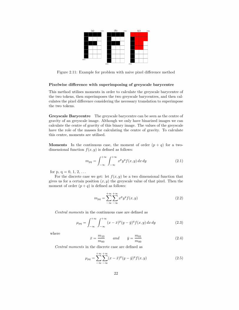
Although the fact of comparing the number of differing pixels to the min-imum number of black pixels gave good results, one problem still persists: itoften happens that two tokens are nearly identical, except for the fact that oneof them has on one of the 4 sides one ore more pixels in addition. This can bedue to noise, blurred printing, problems with binarization, etc. Then it mightbe, that the number of counted different pixels is high, although they vary onlyin one black pixel, as in figure 2.11. The red pixels are all the pixels that differfrom the corresponding pixel in the other token.

21

(a) (b) (c)

(0,0)

(0,0)

(3,5) (3,6)

(0,0)

(3,6)

Figure 2.11: Example for problem with naive pixel difference method

Pixelwise difference with superimposing of greyscale barycentre

This method utilises moments in order to calculate the greyscale barycentre ofthe two tokens, then superimposes the two greyscale barycentres, and then cal-culates the pixel difference considering the necessary translation to superimposethe two tokens.

Greyscale Barycentre The greyscale barycentre can be seen as the centre ofgravity of an greyscale image. Although we only have binarized images we cancalculate the centre of gravity of this binary image. The values of the greyscalehave the role of the masses for calculating the centre of gravity. To calculatethis centre, moments are utilised.

Moments In the continuous case, the moment of order (p + q) for a two-dimensional function f(x, y) is defined as follows:

mpq =

∫ +∞

−∞

∫ +∞

−∞

xpyqf(x, y) dx dy (2.1)

for p, q = 0, 1, 2, . . .For the discrete case we get: let f(x, y) be a two dimensional function that

gives us for a certain position (x, y) the greyscale value of that pixel. Then themoment of order (p + q) is defined as follows:

mpq =

+∞∑−∞

+∞∑−∞

xpyqf(x, y) (2.2)

Central moments in the continuous case are defined as

µpq =

∫ +∞

−∞

∫ +∞

−∞

(x − x)p(y − y)qf(x, y) dx dy (2.3)

wherex =

m10

m00

and y =m01

m00

(2.4)

Central moments in the discrete case are defined as

µpq =

+∞∑−∞

+∞∑−∞

(x − x)p(y − y)qf(x, y) (2.5)

22

wherex =

m10

m00

and y =m01

m00

(2.6)

x and y are the coordinates of the greyscale barycentre in the local coordi-nate system of the token. Central moments are used in the next paragraph forcalculating the central moments of a token.

Our method now calculates the translation that is needed to superimposethe greyscale barycentre of one token to the greyscale barycentre of the othertoken. It then calculates the number of differing pixels.

Because of the rounding operation, we not only checked the pixel differencefor this translation, but also for its 8 neighbouring pixels. The minimum of this8 pixel difference calculations is returned as result.

For our example 2.12 we get for token (a):

xA =m10

m00

=

∑3

0

∑5

0xf(x, y)∑3

0

∑5

0f(x, y)

= . . .

=6 × 0 × 255 + 2 × 2 × 255 + 2 × 3 × 255 + 1 × 4 × 255

(11 × 255) + (13 × 0)

=2295

2805' 1

(2.7)

N.B.: in order to find the barycentre of the black pixels we changed for thecalculation of the moments the value for white to 0 and the value for black to255. The same has been done for all the values of the greyscale scale in case wedon’t have a binary image.

yA =m01

m00

=

∑3

0

∑5

0yf(x, y)∑3

0

∑5

0f(x, y)

= . . .

=1 × 1 × 255 + 1 × 2 × 255 + 3 × 3 × 255 + 1 × 4 × 255 + 4× 5× 255

(11 × 255) + (13 × 0)

=9180

2805' 3

(2.8)

So we get for our greyscale barycentre of token (a) BA(x, y) the coordinatesBA(1, 3). The same way we get the coordinates for our token (b) BB(1, 4).

23

Now we can superimpose the two tokens and we get a pixel difference of4 pixels. In figure 2.12 the greyscale barycentre is coloured in blue. In figure2.12(c) you can see the tokens after superposition. The red pixels are the pixelsthat are not the same for the two tokens. Instead of 11 different pixels we findhere only 4 different pixels.

(b) (c)

(0,0)

(0,0)

(3,5) (3,6)

(0,0)

(3,6)(a)

Figure 2.12: Example for superimposing two tokens

Comparison using moments

Instead of doing the pixelwise comparison, we also tried to compare the momentsof the token to find out whether two tokens are similar or not. The order of thecentral moments we calculated was 2. So we calculated µ00, µ01, µ10 and µ11 forevery token. As µ01 = 0 and µ10 = 0 we only needed to calculated µ00 = m00

and µ11 = m11−xm01 = m11−ym10. This calculations can be found in [GW02].

In this case, two tokens are considered similar if their vector of the two mo-ments is similar. In our case this vector contains µ00 an d µ11. The problemhere is to define when these two vectors are similar and when not. We tried toset the similarity as a threshold: if a the number of differing elements is lessthan the threshold, they are considered similar. We set this threshold to 2.This means that the two elements of vector (a) have to be similar to the twoelements of vector (b). Two elements of the vectors are considered similar, iftheir difference is less than a threshold T. This threshold is fixed by the user.It might be suitable to set this threshold more “intelligent” than by setting itto a fix value.

So in our case two vectors are considered similar if abs(µ01a−µ01b

) < T andif abs(µ11a

− µ11b) < T .

Comparison using Fourier coefficients

The idea behind this method is, not to compare the surface distribution as inthe moments method, but to consider the contour of the character, and thento compare values that have a relation with the contour, instead of comparingvalues that give us only information about the distribution of the pixels.

The idea is to consider the coordinates of the contour pixels of a token asa complex function f(x, y) = x + ıy. Then this function is Fourier transformedin order to get the Fourier coefficients. These coefficients can be interpreted asinformation about the contour of the character. The token representing an “o”

24

will probably have a high part of low frequencies, because there are not a lotof direction changes. So an “o” and an “O” are likely to have similar Fouriercoefficients. This will not be the case for the token representing an “E”. Here alot of high frequencies can be found due to the high frequent change of direction.

So in this method the Fourier coefficients are compared. As only the coeffi-cients representing the low frequencies are interesting to get a rough impressionof the contour, we only compare the coefficients representing low frequencies. Ifthese are similar enough for two tokens, this two tokens are considered as beingsimilar.

The first step is to find the coordinates of the boundary pixels. We used thePavlidis Algorithm [Pav82a].

Pavlidis Algorithm The idea is quite simple: choose a starting point, andthen walk in a fixed direction around the token until you are back at your start-ing point.

The first step is to choose a starting pixel. As this starting pixel should bethe same for two identical tokens we chose the lowest leftmost pixel as startingpixel because it is unique in every token and it is the same for two equivalenttokens.

The easiest way to explain the algorithm is the following: imagine a littleturtle being set on this first starting pixel. The aim of the algorithm is to letthis turtle walk all the way around till it is back on the starting point.

Therefore we need first need to define the directions in which the turtle maylook: because we only check for the four neighbours, we only need to have fourdirections. These are defined as in figure 2.13. Direction 0 points upwards. Theother directions are given counter clock wise: direction 1 will point to the leftof the token, direction 2 will point to the bottom of the token and direction 3to the right side. These directions are relative to the orientation of the token,not to the orientation of the turtle. The direction in which our turtle is looking

(a)

12

30

(b)

12

30

Figure 2.13: An example for a turtle looking in direction 0 (a), and one forlooking in direction 1 (b)

at the beginning is fixed with 0. So the turtle looks up to the upper side of thetoken.

25

We then define the pixels that the turtle will have to check in this order:P1, P2 and P3. P1 is the pixel on the upper left side of our turtle, relative tothe turtles orientation. P2 is the pixel in front of our turtle and P3 if the upperright pixel. P1, P2 and P3 are illustrated in figure 2.14. These pixels are chosenrelative to the orientation of the turtle. The algorithm works as follows:

(b)(a)P1 P2 P3

P1P2

P3

Figure 2.14: Example for the three different pixels that need to be checked forthe Pavlidis algorithm

01 REPEAT

02 IF P1 is a black pixel THEN go to pixel P1

03 ELSE IF P2 is black THEN go to P2

04 ELSE IF P3 is black THEN go to P3

05 ELSE then turn 90 clockwise

06 IF number of consecutive rotations = 4 THEN stop.

07 UNTIL stopped OR current position = starting position

To illustrate the algorithm an example can be found in 2.15. In (a) the turtleis in its starting position. It then moves to its upper left neighbour (b). Fromthis position an direction no black pixel can be reached, so the turtle turns 90clockwise (c). It then moves to P3 (d). These steps are repeated until it reachesthe starting pixel again.The algorithm will return a vector containing the coordinates of the pixels thatare part of the boundary.

Fourier Transform As seen before, the Pavlidis algorithm returns us a vec-tor of the coordinates of the boundary pixels. These pixels can be seen aspair (x0, y0), (x1, y1), . . . , (xk−1, yk−1). Consider the function s(k) = [x(k), y(k)]where x(k) = xk and y(k) = yk. We then can consider s(k) as complex functions(k) = x(k) + ıy(k).

The advantage of this method is to reduce a two dimensional problem to aone dimensional problem.

The Discrete Fourier Transform (DFT) is defined as follows:

a(u) =1

K

K−1∑k=0

s(k)e−ı2πuk/K (2.9)

The calculation of the DFT is done by the Fast Fourier Transform (FFT). Anintroduction about how the FFT works can be found in [Pav82b]. The algo-

26

P2P1

(a) (b)

P1P2

(d)P1 P2 P3

(e)

P2P1

P3

(h)

(f)

P1P2P3

(c)

P2P1 P3

(g)

P1P2P3

P3P3

Figure 2.15: Example for the Pavlidis algorithm for extracting the contour of atoken

rithm gives us as output a vector of all the Fourier coefficients of the currentcontour. The vector is sorted, so that the first entry is equal to a(0), the secondto a(1), etc.

If we have to compare two tokens, t1 and t2, we first calculate the boundaryof the two tokens. Then the boundaries are Fourier transformed. Now we havethe Fourier coefficients of the two tokens and can compare these. We definedtwo coefficients as similar if the following condition is true: |at1(k)−at2(k)| < 1.

In our implemented version of the methods, we coupled the Fourier methodwith the pixelwise method. So the Fourier comparison has not to be too re-strictive. That is why we defined two tokens as similar if 2 out of the 8 firstcoefficients are similar.

Results

The pixelwise method works well but has one big disadvantage: it needs a lot oftime. For every pair of prototype and unanalysed token the difference has to becalculated. And the more prototypes we get, the more pixelwise comparisonshave to be done. This is the reason why pixelwise comparison was not chosen asa first step to find out if two tokens are similar or not. However is was retainedas second step after finding out with a first step that two tokens are potentiallysimilar.

The moments method worked fast but not well enough. There were a lot ofmisclassifications. Also is it difficult to find a good method to decide whether twovectors of moments are similar or not. Due to the fact that the Fourier method

27

worked better, without having to set a lot of parameters, this method wasnot withheld, although it might be possible to get better results if an adaptedmethod for comparing the moments vectors is found.

The method comparing Fourier coefficients works fast if the number of co-efficients to be compared is low. However, if we only compare a few number ofcoefficients the number of misclassified tokens increases. If we compare manycoefficients, this number decreases, but the algorithm becomes slower.

Two steps method

This method is composed of two steps: the first one is a fast Fourier coefficientscomparison method, the second one is the pixelwise comparison method.

01 get contour of token ;

02 do FFT with the contour and get vector of coefficients ;

03 int similar = 0 ;

04 FOR the n first four.coeff. DO

05 IF both coefficients of the two tokens are similar THEN

06 similar++ ;

06 IF (similar > k) THEN

07 compare the two tokens pixelwise ;

08 IF (number of different pixels < l) THEN

10 two tokens are similar

11 ELSE tokens are different

12 ELSE tokens are different

In our case n = 8 and k = 2 gave good results. The problem, that these valuesallow a lot of misclassifications for the Fourier method, is rectified by the pixel-wise comparison. The value for l is can have two values in our case, dependingon whether we have lossless compression l = 0.5 x min(number black pixels ofthe two tokens) or we have lossy compression l = 0.3 x min(number black pixelsof the two tokens). The reason why we have two different values is to allow thelossless compression to misclassify some tokens. This misclassification is undoneby the fact that we save the difference pixels in order to reconstruct the originalimage. In the case of lossy compression no misclassification is allowed, becausethe text will loose its readability if e.g. the “e” is replaced by a “c”.

2.4.3 Lossy/Lossless Compression

The aim of this part of the project was to implement the ability to compress animage without loss of information. This means that the original image had tobe reconstructed without any change of any pixel.

For this reason the residual image has to be modified. The idea is to vir-tually reconstruct the image after compression, and to scan the original imageand the virtually reconstructed pixelwise and to save the differing pixels in theresidual image. So, if a pixel in the reconstructed image differs from the one inthe original image, the concerning pixel in the residual image is set.

28

Instead of really reconstructing the image, we update the residual image bysimply comparing the original tokens with the prototypes that will replace thesetokens.

An example for how this works is given in figure 2.16. The blue pixels shouldbe the greyscale barycentres, but in this case they are not. It is only used tocreate a simple example to illustrate our technique. Let (a) be the prototypeand (b) be the token similar to the prototype. So the token (b) is substitutedby token (a). To calculate the residual image we superpose the tokens so thatthe greyscale barycentres are superposed (blue pixel). As the tokens have notnecessarily the same size, they usually don’t overlap in all their points. There-fore, three cases have to be considered:

1st: we are somewhere in the overlapping area. If the pixel (x, y) of the orig-inal token differs from the pixel (x, y) of the prototype then the pixel(origposX + x, origposY + y) of the residual image is set (it is set to 0,black), where origposX and origposY are the coordinates of the positionof the original token in the original image. When we are reconstructing,we can check if the pixel of the residual image in this position is black andthen we can set the resulting pixel to the inverse of the prototype pixel(black to white resp. white to black).

2nd: if we are in the area of the original token but outside the area of theprototype, then we simply copy the pixel from the original token to theresidual image. These areas aren’t checked while reconstructing. So wesimply have to save all information that these areas contain.

3rd: if we are in the area of the prototype but outside the area of the originaltoken: then we copy the value of the prototype pixel to the residual image.Here we have to save the pixels from the prototype in order to delete themduring reconstruction.

In figure 2.16 the numbers in (d) indicates what case was used to determine thevalue of the pixel.

An example of a residual image can be found in figure 2.17.

2.4.4 Compression of multiple pages with one dictionary

The idea was to increase the compression rate by reutilising one dictionary a forcompressing several pages. The hope was that the number of new prototypes foreach page would tend to zero, the more pages we compressed, and that the onlynew information would be the positions informations and the residual images.

The first step to do is to read such a dictionary and to extract the tokensand save them as new prototypes (as they have already been identified as pro-totypes and because these prototypes are needed to reconstruct the images). Inthe second step the normal image would be read, the tokens extracted and theprogram would continue normally.

29

(a) (b)

Prototype

Original

superposed

(d)

residual image

(c)

3

1

1 1

1 2

2 2

2 2 2 2

2222

3 3

3

3

2

Figure 2.16: Example for updating the residual image

Figure 2.17: Example of a part of a residual image

30

2.4.5 Implementation Details

Saving of prototypes

In a first phase the prototypes were all saved in an image, all prototypes in onerow, one after the other. In order to find the prototypes back we needed anadditional text file containing the bounding boxes of the prototypes. Becauseof this and because of the fact that disk space is wasted due to the differentheights of the prototypes, another format for saving the prototypes had to befound.

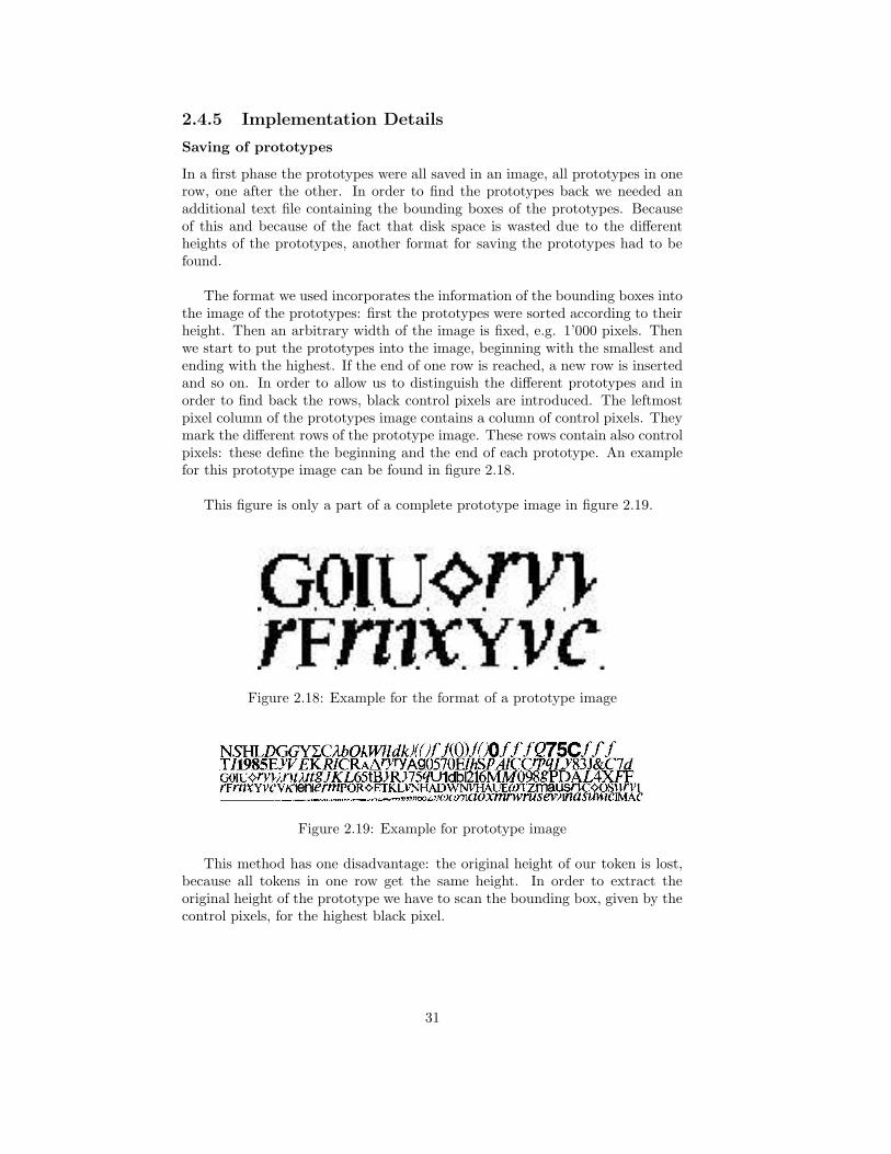
The format we used incorporates the information of the bounding boxes intothe image of the prototypes: first the prototypes were sorted according to theirheight. Then an arbitrary width of the image is fixed, e.g. 1’000 pixels. Thenwe start to put the prototypes into the image, beginning with the smallest andending with the highest. If the end of one row is reached, a new row is insertedand so on. In order to allow us to distinguish the different prototypes and inorder to find back the rows, black control pixels are introduced. The leftmostpixel column of the prototypes image contains a column of control pixels. Theymark the different rows of the prototype image. These rows contain also controlpixels: these define the beginning and the end of each prototype. An examplefor this prototype image can be found in figure 2.18.

This figure is only a part of a complete prototype image in figure 2.19.

Figure 2.18: Example for the format of a prototype image

Figure 2.19: Example for prototype image

This method has one disadvantage: the original height of our token is lost,because all tokens in one row get the same height. In order to extract theoriginal height of the prototype we have to scan the bounding box, given by thecontrol pixels, for the highest black pixel.

31

Substitutions

For reconstruction, we need to know on what coordinates what prototype has tobe put. This prototype is identified by a number. This number is assigned whenit is created. The first prototype found gets the number 0, the second the num-ber 1, etc. These numbers are not saved in the prototype image. It was intendedto get the number out of the position in the prototype image. But now that theprototypes are first sorted and then saved, this method does not work any more.

Therefore we introduced a new text file containing the substitution(s). Inthe case that we don’t use an old dictionary, this means that our dictionary isempty at the beginning of the similarities check, this file only contains a map-ping from the old prototype number to the new number. This new number isthe place of the prototype in the sorted prototype list.

In case we use one dictionary to compress more than one image, we needto be able to reconstruct the original number even after several sorting actions.That is the reason why for every compressed image, a new vector of entries areappended to the substitutions file. A small example for how this works can befound in figure 2.20.

Figure 2.20: Example for the use of the substitutions information

Suppose that image “test1.pgm” has been compressed to “test1pos.txt”,“prototypes1.pgm” and “substitutions.dat”. In the second step the dictionary“prototypes1.pgm” is reused to compress the image “test2.pgm”. Here we getthe new dictionary “prototypes2.pgm”, a new positions data file “test2pos.txt”and the substitutions file is extended with a few new entries.

We now want to reconstruct the image “test1.pgm” by using the “test1pos.txt”and the new dictionary “prototypes2.pgm”. In order to find the original num-ber of the token “3” we take the number of the token ”3”, in this case 4 andsubstitute it with its precedent number, namely 2. Then we go to the firstsubstitution and replace the number 2 by it precedent number, in this case also2. So 2 is the original number of token “3” in the first compression step. Thisworks the same with more than two steps.

In order to distinguish the different entries in the substitutions file and to

32

allow us to find what entries have to be composed, to get the original proto-type number, we needed a unique identifier that tells us what image has beencompressed with what dictionary. In case we are using an existing dictionarywe save the name of the new dictionary (e.g. “prototypes2.pgm”), the name ofthe old dictionary (“prototypes1.pgm”) and the name of the positions data file.In case we are not using an existing dictionary we save the name of the newdictionary file (prototypes image) twice and the name of the positions data file.

Compressing the output files

In order to compress the output files, a script creates a zipped file that containsall the output files needed for reconstruction. These files are the following:

• prototype image: this image is in the “pgm” format

• residual image: this image is compressed as a “TIFF G4” file

• positions data: a text file containing data needed for reconstruction

• substitutions data: a text file containing data needed to find the originalunique number of a prototype (in case of compressing more than one imagewith one dictionary)

2.5 Reconstruction


The aim of this part is to reconstruct the original image (or an image that isquite similar to the original image) out of our saved data:

• Input:- residual image- a text file containing the positions data- substitution data

• Output:- the original image

The algorithm works as follows:

01 extract tokens from prototype image

02 read residual image

03 read positions data

04 read substitutions data

05 IF image compressed with reused dictionary THEN

06 Compose different substitutions steps to one substitution ;

07 ELSE

08 Read the one and only substitution step ;

09 FOR each entry in the positions data DO

10 reconstruct on position x,y the original token by using

33

the concerning prototype and the residual image ;

20 save the output image ;

2.5.2 Composition of the substitutions

As seen before, it may happen that a series of substitutions has to be composedin order to get the original number of the token as it has been saved in the po-sitions text file. To illustrate how this works we will explain it with an exampleof a substitutions file, that can be found in table 2.1.

The starting point of the composition is given by the dictionary name weuse to reconstruct the image, e.g. “pro03.pgm”. The ending point is given bythe positions data file name, e.g. “pos01.txt”. What we need is the number ofthe prototypes as they were in dictionary “pro01.pgm”, to reconstruct image 1.We then try to find a “way” from the beginning to the end. First we substitutethe entries of the 2nd substitution by the ones of the 3rd substitution. Then weonly need the step from “pro02.pgm” to “pro01.pgm”. This step can be done bysubstituting the entries we got in the step before into the entries from the firstsubstitution. So after the last step we have a mapping from the original numberof a prototype in dictionary “pro01.pgm” to the number of this prototype inthe new dictionary “pro03.pgm”.

2.5.3 Lossless compression

If we are using lossy compression we simply put the right prototype on the rightplace. For lossless compression, we have to check the pixels of the residual imagein order to merge the information of the prototype and the residual image toreconstruct the original token.

We have the following information: the place where the prototype has to beplaced and the number of the prototype. Then we scan for all the prototypepixels the concerning pixels in the residual image. Three cases may happen:

1st: IF residual image in (x,y) is white THEN we simply copy the correspond-ing prototype pixel.

2nd: IF residual image in (x,y) is black AND IF concerning prototype pixel iswhite THEN save the pixel as black.

pro01.pgm pro01.pgm pos01.txt. . .



Table 2.1: Example for the entries in the substitutions data file

34

3rd: IF residual image in (x,y) is black AND IF concerning prototype pixel isblack THEN save the pixel as white.

Still there is one unsolved problem with this method: as seen before, it mayhappen that two or more boxes are overlapping. In this case it is not clear whatresidual information belongs to what token. This problem has not been solvedin our method so there will still be differences between the reconstructed imageand the original image. So this method is not lossless but only pseudo-lossless asthere still exist pixels that differ from the original image. This problem can beavoided if the construction of the residual image would be done by comparinga reconstructed lossy image to its original image, and then saving the differingpixels.

35

Chapter 3

Results

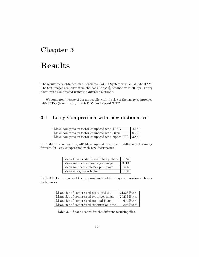
The results were obtained on a Pentium4 2.5GHz System with 512MByte RAM.The test images are taken from the book [Ebb87], scanned with 300dpi. Thirtypages were compressed using the different methods.

We compared the size of our zipped file with the size of the image compressedwith JPEG (least quality), with DjVu and zipped TIFF.

3.1 Lossy Compression with new dictionaries

Mean compression factor compared with JPEG 4.16Mean compression factor compared with DjVu 0.32Mean compression factor compared with zipped TIF 3.86

Table 3.1: Size of resulting ZIP-file compared to the size of different other imageformats for lossy compression with new dictionaries

Mean time needed for similarity check 18sMean number of tokens per image 3713Mean number of classes per image 496Mean recognition factor 7.58

Table 3.2: Performance of the proposed method for lossy compression with newdictionaries

Mean size of compressed position data 21323 BytesMean size of compressed prototyes image 20237 BytesMean size of compressed residual image 614 BytesMean size of compressed substitution data 895 Bytes

Table 3.3: Space needed for the different resulting files.

36

As one can see in table 3.2, the method needs quite a lot of time, nearly 20seconds in average. Compared with JPEG in least quality (table 3.1), it createsfiles that are four times smaller and are better readable than the JPEG versionof the image. But JPEG is not the best method for compressing bi-tone imagesof text. Compared to DjVu, our method gives a file that is three times biggerthan the same image compressed with our method. For zipped TIFF the factoris also about four.

A conclusion that is quite straightforward is, that the compression rate in-creases if the recognition rate increases. This means that we have fewer proto-types and fewer prototypes means less space is needed to save them.

This is also the explanation why the method needs less time if the recogni-tion rate is better: fewer prototypes are found and the new tokens have to becompared fewer times.

It is also clear that the size of the compressed residual image is very small(table 3.3). It contains only a few black lines that can be compressed well withstandard compression techniques.

3.2 Lossless Compression with new dictionaries

Mean compression factor compared with JPEG 1.10Mean compression factor compared with DjVu 0.21Mean compression factor compared with zipped TIF 1.01

Table 3.4: Size of resulting ZIP-file compared to the size of different other imageformats for lossless compression with new dictionaries

Mean time needed for similarity check 8sMean number of tokens per image 3713Mean number of classes per image 274Mean recognition factor 13.83

Table 3.5: Performance of the proposed method for lossless compression withnew dictionaries

Mean size of compressed position data 20197 BytesMean size of compressed prototyes image 11425 BytesMean size of compressed residual image 130527 BytesMean size of compressed substitution data 490 Bytes


In table 3.5 we can see, that the method was faster in the lossless case thanin the lossy case. This is due to the increased recognition rate: the factor ofnew tokens divided by prototypes rose to 13.83. So there are fewer prototypes,

37

and fewer prototypes mean that the program has to compare fewer tokens.

The explanation why we have an increased recognition rate is, that in thiscase the program is allowed to classify tokens wrongly, e.g. an “e” as a “c”.These misclassifications are undone by the residual image. So the size of theresidual image increases and the size of the prototype images decreases. It isnecessary to find an optimum between the number of misclassifications and thesize of the residual image in order to minimise the output files.

The size of our output files increased dramatically. Our method gives ap-proximately the same size as one would obtain with the compressed TIFF file(table 3.2). The DjVu files are in mean 5 times smaller than ours.

The problem with our method is the residual image: it contains a lot of blackpixels, distributed all over the image. These can be compressed very difficultly.This can be seen in table 3.6: the mean size of the compressed residual image isabout 10 times the mean size of the compressed prototypes image. Comparedwith the lossy compression, the size of the residual image increased about 200times.

A method to decrease the number of residual pixels would be to choose anideal prototype such that the difference between all the tokens that are similarto their prototype will be minimal. So the number of residual pixels producedby this prototype will be minimal, and the fewer lonely black pixels there are,the better this image may be compressed.

3.3 Lossy Compression with re-used dictionary

Here one dictionary file is used for 10 images. This has been done twice, withtwo sets of 10 images, in total with 20 images. The size for JPEG, ZIP TIFFand DjVu is calculated by summing up the space needed for each single file.This is compared with our compressed file containing the information for all the10 files. The time and numbers of tokens and number of prototypes are absolutevalues, and no mean values.

Set 1 Set 2Compression factor compared with JPEG 6.74 5.54Compression factor compared with DjVu 0.55 0.42Compression factor compared with zipped TIF 6.32 5.16

Table 3.7: Size of resulting ZIP-file compared to the size of different other imageformats for lossy compression with re-used dictionaries

In table 3.8 we can see, that the recognition rate is higher than in the lossycase without re-used dictionary, and its compression rate is also better (table3.3). So the re-use of a dictionary has had the impact we had planned, namelyto increase the recognition rate and to increase the compression rate. But com-pared to the time needed to compress this 10 images, this improvement is not

38

Set 1 Set 2Total time needed for similarity checks 13m44s 13m26sTotal number of tokens 37355 38062Total number of classes 1675 1548Recognition factor 22.3 24.59

Table 3.8: Performance of the proposed method for lossy compression withre-used dictionaries

Set 1 Set 2Size of compressed position data files 251860 Bytes 251593 BytesSize of compressed prototyes image 67159 Bytes 61876 BytesSize of compressed residual image files 6259 Bytes 6145 BytesSize of compressed substitution data 7689 Bytes 7036 Bytes


relative to computational effort. It is simply too slow. The compression rate iseven better than the rate obtained by compressing the images one by one. Butit is still no match for DjVu, even if we simply sum up the size of the singlecompressed files DjVu files.

We can see here, that in the lossy case, the space needed by the residualimages is nearly neglectable (table 3.9). Even the substitution file is larger thanall the residual images.

3.4 Lossless Compression with re-used dictio-nary

Here one dictionary file is used for 10 images. This has been done twice, withtwo sets of 10 images, in total with 20 images. The size for JPEG, ZIP TIFFand DjVu is calculated by summing up the space needed for each single file.This is compared with our compressed file containing the information for all the10 files. The time and numbers of tokens and number of prototypes are absolutevalues, and no mean values.

Set 1 Set 2Compression factor compared with JPEG 1.07 1.08Compression factor compared with DjVu 0.21 0.20Compression factor compared with zipped TIF 1.00 1.00

Table 3.10: Size of resulting ZIP-file compared to the size of different otherimage formats for lossless compression with re-used dictionaries

We can see in table 3.11, that even in this case our compression rate isnot good, although the recognition rate for ten images is very high, due toa probably large number of misclassifications. Zipped TIFF and JPEG are,

39

Set 1 Set 2Total time needed for similarity checks 4m32s 6m37sTotal number of tokens 37355 38062Total number of classes 777 740Recognition factor 48.08 51.44

Table 3.11: Performance of the proposed method for lossless compression withre-used dictionaries

Set 1 Set 2Size of compressed position data files 223529 Bytes 225030 BytesSize of compressed prototyes image 30292 Bytes 28161 BytesSize of compressed residual image files 1423917 Bytes 1428918 BytesSize of compressed substitution data 3695 Bytes 3405 Bytes


compressed each file for its own, nearly as big as the file we get with our method(table 3.4). This is due to the residual image that is too large (table 3.12). Asone can see, the major part of the space needed is used by the residual images.Compared with the sum of the sizes of the single DjVu Files this method bringsno advantage for the compression rate.

40

Chapter 4

Conclusion & OpenProblems

In this project thesis a token-based compression method has been implemented.The first step, consisting of binarization, has been done with an adaptive localthresholding algorithm. Then the connected components have been identifiedby a labelling method that uses a union-find data structure. After this, a naivenoise reduction step deletes the boxes smaller than a certain threshold.

The main step consists of grouping the tokens together, so that similar to-kens are in the same class. Pixelwise comparison, moments comparison andFourier coefficients comparison of the boundary pixels have been tried. A com-bination of Fourier coefficients comparison and pixelwise comparison has beenused.

The method allows to compress lossy and lossless. It also has the ability tore-use a dictionary (an image file containing prototypes in a certain format) inorder to compress a number of pages with the same dictionary.

The last step is the reconstruction of the image out of the files created inthe compression step.

Compared to JPEG an compressed TIFF our method has in some cases abetter compression rate, although it does not reach the efficiency of the DjVuformat .

One problem is the size of the residual image for lossless compression. It getstoo big due to the fact that the choice of our prototype is not ideal. More workshould be done to find a way to optimise the choice of the prototype. Maybe itwould be useful to save a token as prototype that does not exist in the imagebut that has the least distance to all tokens similar to it.

In addition, the different parameters may be chosen in a more intelligentway. Especially the parameter of the allows pixel difference has in importantrole. It should be chosen to minimise the total size of the residual image and

41

the size of the prototype image.

An other problem is the time the method needs: even though the Fouriermethod works faster than only comparing the tokens pixelwise, it has the prob-lem that the larger the number of prototypes gets, the more time it need, becauseit has to compare every unknown token with all the prototypes. This also ex-plains why the method reusing dictionaries works so slowly.

42

Bibliography

[AN74] R.N. Ascher and G. Nagy. A Means for Achieving High Degree ofCompaction on Scan-Digitized Printed Text, volume C-23, No. 11,pages 1174–1179. November 1974.

[BHH+98] L. Bottou, P. Haffner, P. Howard, P. Simard, Y. Bengio, and Y. Le-Cun. High quality document image compression with DjVu. Journalof Electronic Imaging, Vol. 7(No. 3):410–425, July 1998.

[Dav97] E. Roy Davies. Machine Vision: theory, algorithms, practicalities,page 97ff. Academic Press, San Diego, 2nd edition, 1997.

[Ebb87] Heinz-Dieter Ebbinghaus. Ω-Bibliography of Mathematical Logic,volume 3. Springer Verlag, Berlin, 1987.

[GW02] Rafael C. Gonzalez and Richard E. Woods. Digital Image Processing.Prentice Hall, Upper Saddle River, NJ, 2nd edition, 2002.

[Pav82a] Theo Pavlidis. Algorithms for Graphics and Image Processing, page142ff. Springer Verlag, Berlin, 1982.

[Pav82b] Theo Pavlidis. Algorithms for Graphics and Image Processing, page28ff. Springer Verlag, Berlin, 1982.

[Rei] Reichelt. Reichelt Katalog 2005/1.

43

project thesis token-based compression -...

Documents