project title: dielectric, thermal and mechanical

P a g e | III

University of Southern Queensland

Faculty of Engineering and Surveying

Project Title: Dielectric, thermal and mechanical

properties of sawdust reinforced epoxy composites

post-cured in microwaves

A dissertation submitted by

Ping Tai

In fulfillment of the requirements of

Bachelor of Engineering (Electrical)

October 2010

P a g e | IV

P a g e | V

P a g e | VI

ABSTRACT

To process composites, post-curing with heat is often required in order to achieve the

desired heat distortion temperature (HDT). Post-curing the composites with

conventional oven would often take 6 or 8 hours. However, if the composites are post-

cured in a microwave oven, it only requires a few minutes. Hence, the aim of the project

is to investigate the suitability of microwave for material processing. Epoxies are

polyethers and they are widely used to produce coatings, structural adhesives because

they have excellent adhesion and low cure shrinkage. Epoxies are also good dielectric

and have been used to manufacture printed circuit boards (PCB).

The main objectives of this project are:

• To produce specimens with different percentage by weight of sawdust.

• To measure the loss tangent and dielectric constant of the specimens.

• To measure the tensile strength of the specimens.

• To measure the glass transition temperature of the specimens

• To consider both of the material costs and the test results to recommend

the best specimens for different industrial applications.

This report has found that the sawdust reinforced epoxy resins have higher Young’s

modulus, higher dielectric constant but lower tensile strength and yield strength. The

loss tangents of the sawdust reinforced epoxy resins were slightly higher than the loss

tangents of pour epoxy resins. Hence, the sawdust reinforced epoxy resin is slightly

more efficient to be post-cured in microwave than pure epoxy resin. This report has also

found that oven cured epoxy resins have the lowest dielectric constant, the lowest loss

tangent, and the highest glass transition temperature. Hence, oven cured epoxy resin is

the best candidate for making PCBs.

P a g e | VII

Acknowledgements

I would like to take this opportunity to acknowledge my supervisors, Dr Harry Siu-

Lung Ku and Dr Francisco Cardona for their guidance and wisdom throughout this

project. Many thanks and sincere appreciation for their patience, understanding, and

helpful advice.

I also would like to thank Mr Mohan Trada for assisting me with the microwave post

curing. His safety advice and expert instructions were invaluable in helping me to

successfully compete this project.

Finally, I respectfully acknowledge Toowoomba Timber Mart for providing me with the

free sawdust for this project.

P a g e | VIII

Table of Contents ASSIGNMENT COVER SHEET………………………………………………..............I

DISSERTATIOB SUBMIT FORM……………………………….................................II

TITLE PAGE………………………………………………….….................................III

LIMITATION OF USE ………………………………………………………..............IV

CANDIDATES CERTIFICATION ………………………………………………......V

ABSTRACT………………………………………………………...............................VI

ACKNOWLEGEMENTS……………………………………….................................VII

LIST OF FIGUERS……………………………………………………………..…….XII

LIST OF TABLES…………………………………………………………..………XVII

LIST OF APPENDICES……………………………………………………............XVIII

NOMENCLATURE ……………………………………………………….……..….XIX

1. INTRODUCTION ...................................................................................................... 1

1.1 Introduction ............................................................................................................. 1

1.2 Project Objectives .................................................................................................... 1

1.3 Environmental implications ..................................................................................... 2

1.4 Safety ....................................................................................................................... 2

1.5 The Resource analysis .............................................................................................. 4

2. LITERATURE REVIEW ............................................................................................... 5

2.1 Epoxy resins ............................................................................................................. 5

2.1.1 Types of epoxy resins ........................................................................................ 5

2.3 Fillers ........................................................................................................................ 8

2.4 Glass transition temperature ................................................................................... 8

2.5 Moisture absorption of resins ................................................................................. 9

2.6 Yield strength ......................................................................................................... 11

2.7 Tensile strength ..................................................................................................... 12

2.8 Young’s modulus .................................................................................................... 12

2.9 Microwaves ............................................................................................................ 13

2.9 .1 Microwave fundamentals ............................................................................... 13

2.9.2 Microwave interaction with matters .............................................................. 14

2.9.3 Thermal runaway ............................................................................................ 20

P a g e | IX

2.9.4 Variable Frequency Microwave ....................................................................... 22

2.9.5 Wall loss ........................................................................................................... 23

2.10 Permittivity Measurement .................................................................................. 23

2.11 Wave Guide ......................................................................................................... 26

2.12 Cut-off frequencies .............................................................................................. 27

2.13 Work of others ..................................................................................................... 31

3. METHODOLOGY .................................................................................................... 33

3.1 Experimental equipment specifications ................................................................ 33

3.1.1 Microwave oven .............................................................................................. 33

3.1.2 Infra red handheld thermometer .................................................................... 33

3.1.3 Tensile test machine Test machine ................................................................. 33

3.1.4 Loss tangent measuring devices...................................................................... 34

3.2 Sawdust sifting ....................................................................................................... 34

3.3 Moulds preparation ............................................................................................... 35

3.4 Mixing the samples ................................................................................................ 37

3.5 Specimens cured in room temperature ................................................................ 37

3.6 Dimension of Specimens ....................................................................................... 38

3.7 Post-cure in the microwave oven .......................................................................... 39

3.8 Post-cure in conventional thermal oven ............................................................... 41

3.9 Tensile test ............................................................................................................. 41

3.10 Dielectric constant and loss tangent measurement ............................................ 43

3.11 Possible measurement errors .............................................................................. 47

3.12 Dynamic Mechanical Analysis (DMA) test ........................................................... 48

3.13 Microscope Analysis ............................................................................................ 52

4. RESULTS AND DISCUSSION ................................................................................... 53

4.1 Loss tangent and Dielectric constant test results .................................................. 53

4.1.1 The loss tangent measurement ....................................................................... 53

4.1.2 The parallel capacitance .................................................................................. 59

4.1.3 Dielectric constant measurement ................................................................... 60

4.2 DMA test results .................................................................................................... 65

4.2.1 DMA test summary.......................................................................................... 73

4.3 Tensile test results ................................................................................................. 77

P a g e | X

4.3.1 Example calculation ......................................................................................... 77

4.3.2 Test results for the composites filled with 300 μm sawdust .......................... 79

4.3.3 Test results for the composites filled with 425 μm sawdust ............................. 83

4.3.4 Test results for the composites filled with 1180 μm sawdust ........................ 86

4.4 Microscope inspection results ............................................................................... 91

4.5 Cost Analysis .......................................................................................................... 97

4.6 Industrial applications ........................................................................................... 98

5. CONCLUSIONS ...................................................................................................... 99

5.1 Introduction ........................................................................................................... 99

5.2 Conclusions ............................................................................................................ 99

5.2.1 Loss tangent and Dielectric constant measurement ...................................... 99

5.2.2 DMA test ........................................................................................................ 100

5.2.3 Tensile test .................................................................................................... 100

5.2.4 Microscope inspection .................................................................................. 100

5.2.5 Industrial applications ................................................................................... 101

5.3 Further Research and Recommendations ........................................................... 101

APPENDIX A............................................................................................................ 102

A.1 – Project Specification ......................................................................................... 102

APPENDIX B ............................................................................................................ 104

B.1 High performance epoxy resins ........................................................................... 104

APPENDIX C ............................................................................................................ 109

C.1 Tensile test results ............................................................................................... 109

P a g e | XI

LIST OF FIGURES

Figure 2.1: High-voltage bushing cast from cycloaliphatic epoxy……………………...6

Figure 2.2: Schematic of crosslinking of epoxy using amine harder……………………7

Figure 2.3: Moisture enhancement effect on thermal spiking for a series of carbon fiber unidirectional laminates………………………………………………………………...10

Figure 2.4: Electromagnetic wave representation……………………………………...13

Figure 2.5: Predicted power- temperature response curve for an alumina sphere…….21

Figure 2.6: The field inside an oven with a potato at the centre of one side…………..22

Figure 2.7: The field inside a microwave oven with a potato at one corner…………...22

Figure 2.8: The phase and magnitude of the electric field at resonant frequency recorded by microwave network analyser………………………………………………………..25

Figure 2.9: The Configuration of testing equipments for Cavity Method …………….26

Figure 2.10: Microwave oven…………………………………………………………..27

Figure 2.11: Coordinate system for rectangular waveguide …………………………...30

Figure 2.12 Cut-off frequencies for different transmission modes…………………….31

Figure 3.1: 425 μm sifter used for sifting sawdust ……………………………………34

Figure 3.2: The mould for casting tensile test samples………………………………...36

Figure 3.3: The mould used for casting the samples for loss tangent measurement…..37

Figure 3.4: The specimen curing at room temperature…………………………………38

Figure 3.5: The samples cut by saws …………………………………………………..39

Figure 3.6: The fly-ash removal reinforced microwave oven…………………………40

Figure 3.7: The infra red handheld thermometer..............…………………………….40

Figure 3.8: Universal Test machine……………………………………………………42

Figure 3.9: Electronic vernier caliper…………………………………………………..42

Figure 3.10 Loss tangent measurement equipment set-up …………………………….44

P a g e | XII

Figure 3.11: (a) equivalent circuit for the sample under test (b) phasor diagram ……..45

Figure 3.12: Edge effects in a parallel plate capacitor………………………………....47

Figure 3.13: Airgap effects……………………………………………………………..48

Figure 3.14: The DMA test results for naturally cured epoxy resins reinforced with 10%

425 μm sawdust ………………………………………………………………………..50

Figure 3.15: DMA instrument …………………………………………………………51

Figure 3.16: The optical microscope used in this project………………………………52

Figure 4.1: Comparison of loss tangent from different curing method of pure epoxy

resins …………………………………………………………………………………...54

Figure 4.2: Comparison of loss tangent from different curing method of epoxy resins

reinforced with 5% 425 μm sawdust ……………………………………………..……55


reinforced with 10% 425 μm sawdust …………………………………………………55


reinforced with 15% 425 μm sawdust …………………………………………………56

Figure 4.5: Comparison of loss tangent for varying percentage of sawdust cured at room

temperature……………………………………………………………………………..57

Figure 4.6: Comparison of loss tangent for varying percentage of sawdust cured in

microwave……………………………………………………………………………...58

Figure 4.7: Comparison of loss tangent for varying percentage of sawdust cured in

oven………………………………………………………………………………….…58

Figure 4.8: Comparison of capacitance for oven cured epoxy resins with varying

percentage of sawdust ………………………………………………………………….59

Figure 4.9: Comparison of capacitance for varying percentage of sawdust ………......59

Figure 4.10: Comparison of capacitance for microwave cured epoxy resins with varying

percentage of sawdust…………………………………………………………….........60

P a g e | XIII

Figure 4.11: Comparison of dielectric constant for oven cured epoxy resins with varying

percentages of sawdust…………………………………………………………………61

Figure 4.12: Comparison of dielectric constant for epoxy resins cured at room

temperature and reinforced with varying percentage of sawdust ………………...……62

Figure 4.13: Comparison of dielectric constant for microwave cured epoxy resins with

varying percentage of sawdust..………………………………………………………..63

Figure 4.14: Comparisons of the dielectric constant for neat epoxy resins…………....63

Figure 4.15: Comparisons of the dielectric constant for epoxy resins reinforced with 5%

sawdust…………………………………………………………………………………64

Figure 4.16: Comparisons of the dielectric constant for epoxy resins reinforced with

10% sawdust…………………………………………………………………………....64

Figure 4.17: Comparisons of the dielectric constant for epoxy resins reinforced with

15% sawdust……………………………………………………………………………65

Figure 4.18: DMA test results for naturally cured epoxy resins reinforced with 5% 425

μm sawdust…………………………………………………………………………….66

Figure 4.19: DMA test results for microwave cured epoxy resins reinforced with 5%

425 μm sawdust………………………………………………………………………...66

Figure 4.20: DMA test results for oven cured epoxy resins reinforced with 5% 425 μm

sawdust……………………………………………………………………………..…..67


μm sawdust…………………………………………………………………………….68


425 μm sawdust………………………………………………………………………..68

Figure 4.23: DMA test results for oven cured epoxy resins reinforced with 10% 425 μm

sawdust…………………………………………………………………………………69


μm sawdust…………………………………………………………………………….70

P a g e | XIV


425 μm sawdust………………………………………………………………….……..70

Figure 4.26 DMA test results for oven cured epoxy resins reinforced with 15% 425 μm

sawdust……………………………………………………………………………...….71

Figure 4.27: DMA test results for naturally cured epoxy resins………………….……72

Figure 4.28: DMA test results for microwave cured neat epoxy resins………………..72

Figure 4.29: DMA test results for oven cured pure epoxy resins………………………73

Figure 4.30: Glass transition temperature of epoxy resins……………………………..75

Figure 4.31: Storage modulus of epoxy resins………………………………………....76

Figure 4.32: Loss modulus of epoxy resins…………………………………………….76

Figure 4.33: the load and extension curve for the specimen 3 of 10% 425μm sawdust

sample set………………………………………………………………………………77

Figure 4.34: Young’s modulus versus percentage of 300 μm sawdust …………….….81

Figure 4.35: Tensile strength versus percentage of 300 μm sawdust ………………….82

Figure 4.36: 0.05% Offset yield strength versus percentage of 300 μm sawdust ……..82

Figure 4.37: Young’s modulus versus percentage of 425 μm sawdust ………………..84

Figure 4.38: Tensile strength versus percentage of 425 μm sawdust…………………..85

Figure 4.39: 0.05% Offset yield strength versus percentage of 425 μm sawdust…...…86

Figure 4.40: Tensile strength versus percentage of 1180 μm sawdust………….…......87

Figure 4.41: Young’s modulus versus percentage of 1180 μm sawdust…………….…88

Figure 4.42: 0.05% Offset yield strength versus percentage of 1180 μm sawdust…….89

Figure 4.43: Comparison of Young’s modulus for 300 μm, 425 μm and 1180 μm

sawdust.………………………………………………………………………………...90

Figure 4.44: Comparison of Young’s modulus for 300 μm, 425 μm and 1180 μm

sawdust…………………………………………………………………………………90

P a g e | XV

Figure 4.45: Comparison of 0.05% offset yield strength for 300 μm, 425 μm and 1180

μm sawdust……………………………………………………………………………..91

Figure 4.46: sample 1 of the epoxy resins reinforces with 5% 425 μm sawdust at a

magnification of 67 times………………………………………………………………92






magnification of 67 times……………………………………………………………....94


magnification of 67 times……………………………………………………………....94


magnification of 67 times…………………………………………………………..…..95



Figure 4.53: sample 3 of the epoxy resins reinforces with 16.7% 1180 μm sawdust at a



magnification of 67 times…………………………………………………………..…..97

P a g e | XVI

LIST OF TABLES

Table 2.1: Effect of thermal spiking and moisture condition on the primary (Tg1) and

secondary (Tg2) tanδ peaks for advanced epoxy resin system………………………...11

Table 2.2: Dielectric properties of foods and other materials of 2.45 GHz at 20 oC…..18

Table 2.3: Dielectric properties of some materials…………………………………..…19

Table 2.4: Dielectric properties of selected materials………………………………….20

Table 4.1: DMA test results…………………………………………………………….74

Table 4.2: Row data record by computer………………………………………………79

Table 4.3: Processed mean values of the test results for samples reinforced with 300 μm

sawdust ………………………………….....................................................................80

Table 4.4: Processed mean values of the test results for samples reinforced with 420 μm

sawdust ………………………………………………………………………………...83

Table 4.5: Processed mean values of the test results for samples reinforced with 1180

μm sawdust …………………………………………………………………………….86

P a g e | XVII

LIST OF APPENDICES Appendix A A.1 Project specification Appendix B B.1 The epoxy family Appendix C C.1 Tensile test results

P a g e | XVIII

Nomenclature

Glossary of Terms

TM - Transverse magnetic wave

TE - Transverse electric wave

TEM - Transverse electromagnetic wave

HDT - Heat distortion temperature

DMA - Dynamic mechanical analysis

PCBs - Printed circuit boards

P a g e | 1

1. INTRODUCTION

1.1 Introduction

Composites have the great flexibility of being able to be modified with their material

properties such as electrical, mechanical and chemical. Hence, they are being

increasingly manufactured to suit different applications in different engineering

industries. To process composites, post-curing with heat is often required in order to

achieve the desired heat distortion temperature (HDT). Post-curing the composites with

conventional oven would often take up to 6 or 8 hours. However, if the composites are

post-cured in a microwave oven, it only requires a few minutes. This significant

reduction in production time means increased productivity and therefore more profit

for the manufacturers. However, there is a major problem in using microwave to heat

up the composites. That is the microwave oven cannot heat up composites evenly by

itself. Uneven heating produced inside the material would cause cracks or distortion to

emerge in the object which would greatly compromise the mechanical strength of the

material. This project will demonstrate the advantages and capability of the microwave

oven in material processing by producing the well post-cured composites.

1.2 Project Objectives

The aim of this project is to produce a range of epoxy resins with different percentages

by weight of sawdust as filler. The result of this project is to demonstrate the effect on

dielectric, thermal and mechanical properties of the final product by adding different

percentage of sawdust and the cost reduction by using cheaper filler such as sawdust.

The objectives of the project are:

1. To research information about tensile properties of sawdust filled epoxy resin

and how they are affected by microwaves. This will help to develop a

comprehensive understanding of the physical principle behind microwave

heating, and the understanding of the bonding mechanisms of composite

materials.

2. To produce specimens with different percentage by weight of sawdust.

P a g e | 2

3. To post-cure the specimens with microwaves.

4. To conduct a test to measure the loss tangent of the specimens. This test would

help to determine the suitability of the composites to be post-cured in

microwave oven.

5. To conduct a Dynamic Mechanical Analysis (DMA) test to measure the glass

transition temperature.

6. To implement tensile test on the specimens by following the instructions of

AS1145.4 (2001).

7. To analyse the test results.

8. To perform a cost analysis, that will provide evidence to prove sawdust filled

composites are more cost effective in comparison to the pure epoxy resin

products.

9. To consider both of the material costs and the test results to recommend the best

specimens for different industrial applications.

10. To suggest possible solution to minimise defects.

1.3 Environmental implications

To protect the environment, the disposal method at the end of the life cycle of the products should be

seriously considered. It is better to develop some methods that can decompose the epoxy composites

other than a simple landfill.

1.4 Safety

Similar to other electrical equipments, there is a potential hazard for electrical shock

due to both the insulation failure of the components inside the equipment, and the

earthing connection failure.

Many people misperceived microwave like other ionizing radiation sources such as x-

ray can cause genetic mutation. Meredith (1998, p. 22) clarified microwave radiation is

P a g e | 3

not an ionizing radiation. It has the effect on human bodies no more than producing

heat.

According to Australia Standards AS60335.2.25 (2002, p26), the microwave leakage

from the oven should be less than 50 W/m2 at the distance of 50 mm from the external

surface of the oven.

Epoxy resin and hardeners have moderate chemical hazards to human body. Vapors of

epoxy can cause allergic reaction to human lungs. People who breathe in these vapors in

long term can develop occupational asthma (California Department of Public Health

1989).

Skin contacts with epoxy resin and hardener can cause skin reaction such as redness,

swelling and itching on the area of contact, these symptoms could continues for a few

days then disappear. The most dangerous situation is the resin or the hardener contacted

with eyes, as these chemicals can cause severe damage to the eyes.

To avoid the potential chemical hazards, people should ensure a good ventilation

condition for the working environment. Gloves, goggles and masks should be worn

during the experiment. According to the manufacturer’s (ATL composites Pty Ltd)

manual, in the occurrence of eye contact, the eyes should be immediately flushed with

running water for a minimum of 15 minutes and then seek medical advice. Also if

people accidently swallow resins, please don’t try to induce vomiting and immediately

seek medical assistance. If people swallow hardeners, also do not induce vomiting, and

drink plenty if milk or water and seek professional medical advice. Furthermore, if skin

contact happened, the contaminated clothing should be removed and the affected area of

the skin should be washed with ATL’s 845 hand cleaner and running water.

In addition to the project specified personal protection equipment, fully enclosed

footwear, and long sleeve shirt should also be worn to provide better protection to

against the unpredicted accidents. As a good practice for conducting experiments, the

P a g e | 4

bench should be always kept clear and clean. Do not bring food and drinks into the

laboratory.

1.5 The Resource analysis

In this experiment, the requirement is to mix the resin with three different sizes of

sawdust. The required sizes for sawdust are 300 μm, 425 μm and 1180 μm respectively.

For each mixture of different size sawdust, three different specimens with different

percentage by weight of sawdust which are 5%, 10% and 15% are required to be

produced. Therefore there are total nine specimens need to be produced to complete

this project. Each sample required 420 g R246TX epoxy resin and 105 g H126

hardener, multiply these numbers by nine, the total epoxy required for the experiment is

3780 g and total hardener is 945 g. The experiment also required 217.21 g of 300 μm,

425 μm and 1180 μm sawdust for each. The sawdust has been acquired from

Toowoomba Timber Mart which is a local timber mill, free of cost. In order to separate

sawdust into required sizes, three corresponding sifters which are provided by the

Centre for Excellence in Engineered Fiber Composites (CEEFC) are used. The epoxy

resins and the hardener are purchased from ALT Composites Pty Ltd. The funding for

purchasing the resins, hardeners, and microwave oven and personal safety equipments

is provided by University of Southern Queensland. Three 30 cm by 20 cm alumina trays

were purchased from BigW Supermarket as the casting moulds. The tensile test

equipment and the instrument to measure the dielectric property of the materials were

provided by USQ.

P a g e | 5

2. LITERATURE REVIEW

2.1 Epoxy resins

Epoxies are polyethers and they are widely used to produce coatings, structural

adhesives because they have excellent adhesion and low cure shrinkage. Moreover,

Epoxy resins are also excellent dielectrics and heat conductors. These properties make

them an ideal material for making printed circuit boards. As the epoxy resins often have

smooth finishing, they are also used in making the rotor blades of wind turbines. In

addition, epoxy resins are also extensively used to make aircraft,, oil rigs, chemical

storage tanks and high speed boats because of their outstanding chemical resistance.

Epoxy resins usually exist in two states. The liquid state of epoxy resins are mainly for

storing purpose. When the epoxy resins mix with the hardeners, the chemical cross links

would be formed between these two chemicals and the mixtures will turn into a hard

solid state. This hardening process is called curing, and it is irreversible. It is quite often

to find that there are some of the chemicals in the mixture remain unreacted. The extent

to which the curing reaction approaches completion is called the degree of cure

(Pritchard 1999, p.13). This incompletion of the chemical reaction would affect the

physical properties of the composites. Hence, in order to facilitate the reaction to

approach 100% completion, it often requires to further process the composite by heating

it up in several steps. This process is called post-cure. Post-curing can improve the

moisture resistance and physical strength of the composites, but excessive post-curing

could increase the brittleness of the composites and the risk of decomposition of the

composites.

2.1.1 Types of epoxy resins

There are many members in the family of epoxy resins. One of the important members

is the diglycidylether of bisphenol A (DGEBA). It has been the popular choice to the

industry because of its fluidity, physical strength after curing and cheap purchasing

P a g e | 6

price. On the other hand, it has relatively low value of Tg less than 120oC. Furthermore,

the cycloaliphatic epoxies which are also important members of the family have

extraordinary arc-track resistance to against the high voltage breakdown. Hence,

cycloaliphatic resins are used to cast the high voltage bushing. Figure 2.1 shows typical

high-voltage bushings made from cycloaliphatic epoxy busing.

Figure2.1: High-voltage bushing cast from cycloaliphaatic epoxy (Harper 1992, p. 6.14)

There are several hardeners available in the market. One of the widely used hardener is

aliphatic amines. Comparing with other hardeners, aliphatic amines require lower

curing temperature. Aliphatic amines, such as diethylenetriamine (DETA),

dimethylaminopropylamine and diethylaminopropyllamine, can cure epoxies at room

temperature. However, these chemicals tend to absorb the moisture from the air, and

hence slow down the curing process. Another disadvantage of this hardener is that there

will be a large amount of heat released from the chemical reaction between the epoxy

resins and the hardener. Hence, aliphatic amines are only used to cure small amounts of

epoxy resins to avoid overheating the composites. Another type of hardener is aromatic

amines. Aromatic amines include metaphenylenediamine (MPDA) and methylene

dianiline (MDA) are solid at room temperature. The composites which are made from

P a g e | 7

epoxy resins and aromatic amines have the highest physical properties in the epoxy

system. However, in recent years, aromatic amines has been found to be a carcinogen

(Harper, 1992), thus the use of aromatic amines is prohibited. Moreover, some acids

and anhydrides are also used as hardeners to cure epoxies. The composites made from

epoxy resins and acids and anhydrides can be used for high temperature applications.

Figure2.2: Schematic of crosslinking of epoxy using amine harder (Ku 2000 et al.)

Figure 2.2 demonstrates the chemical reaction taking place between epoxy resins and

hardeners. The epoxy at the top left corner of Figure 2.2 represents a molecule of the

DGEBA. The amine hardener at the top left corner represents a molecule of DETA. As

P a g e | 8

shown in Figure 2.2, every molecule of amine hardener has two reactive hydrogen.

Each of the hydrogen will react with one epoxide group, hence two epoxy molecules are

bound together via the hardener. This process is known as cross-linking. A distinctive

advantage of this type of polymerization is that the hardener becomes part of the

composites, and there are no products of condensation being produced. Since the

physical size change on this type of polymerization is minimal, the shrink rate is

minimized. High shrinkage could lead to the distortion of the final product and hence

reduce the physical strength of the final product.

2.3 Fillers

Fillers are often added into the epoxy composites to modify or improve different

properties of the composites. For example, carbon fibers as fillers can increase the

chemical resistance of the epoxy composites. Glass powder can increase the moisture

resistant of the epoxy composites. The variety of sawdust used for this project can

increase the physical strength of the epoxy composites. Metal powders, such as

aluminum, silver and copper, can increase the electrical and thermal conductivity of the

composites. Fillers normally do not have chemical reaction with the epoxies. To be

considered as good fillers, they should stay in suspension in the mixtures and have low

cost.

2.4 Glass transition temperature

Glass transition refers to a polymer undergoes a reversible transformation from a brittle

and rigid glass-like state to a viscous rubber-like state. This transition usually takes

place over a range of temperature (Harper,1992). The glass transition temperature Tg is

the temperature in the center of the range. When the temperature is lower than the glass

transition temperature, the material would become glassy. On the other hand, if the

temperature is higher than the Tg, the material would tend to be rubber like. The change

of the physical states will result in rapid change of the physical, mechanical, electrical

and thermal properties of the materials. The content of moistures can greatly reduce the

P a g e | 9

value of Tg. Harper (1992, p.21) motioned that for each 1% moisture absorbed by the

epoxy resin, the Tg will be lowered by 20oC. On the other hand, the glass transition

temperature can be increased from the cross-linking reaction, as the reaction terminates

the free rotation of the end groups.

2.5 Moisture absorption of resins

Resins often tend to absorb moisture from air. As stated by Pritchard (1999), there are

four factors can affect the moisture absorption of resins. The four factors are the

polarity of the molecular structure, degree of crosslinking, degree of crystallinity and

degree of curing. The degree of curing usually indicates the number of monomers (resin

residuals) and hardeners. A recent study also found a rapid raise in temperature could

enhance the moisture absorption of epoxy resins. Figure 2.3 shows the result of the

moisture absorption study. The experiments carried out with several different resins in

a wet environment. The temperature raised from 50 ℃ to 200℃, and most of the under

test specimens reached the their maximum of moisture absorption at 150 ℃ , then

continually fell down as the temperature increased.

The increasing moisture content results in reduction of glass transition temperature of

the epoxy resins. Table 2.1 shows the relationship between the moisture content and the

glass transition temperature. As shown in Table 2.1, when the moisture content

increased from 0% to 1.26 % by weight, the primary glass transition temperature

decreased from 222 ℃ to 198℃. One possible explanation for the moisture absorption

enhancement is that the sudden change in temperature could create microcracks within

the body of the samples. Once the microcracks existed, the moisture content tends to

invade into these tiny spaces. In this project, the process of post-curing in microwave

was originally carried out with a glass of water placed in the microwave oven to prevent

the sample from overheating. However, the consequence of reconsidering the effect of

moisture content on glass transition temperature discussed above, the samples were

reprocessed in the microwave oven with the glass of water removed.

P a g e | 10

Figure 2.3 (a) Moisture enhancement effect on thermal spiking for a series of carbon fibre

unidirectional laminates; ●, Narmco Rigidite 5245C; □, Fibredux 927 and 𝛁, Fibredux 924C. (b)

Moisture enhancement on thermal spiking for a range of matrix resins; ● base epoxy resin-924E; ■,

thermoplastic modified epoxy matrix resin-924T; ○, calculated matrix and composite-924C

(normalised); and ⨁, 924C composite. (Pritchard 1999, p.87)

P a g e | 11

Table 2.1: Effect of thermal spiking and moisture condition on the primary (Tg1) and secondary

(Tg2) tanδ peaks for advanced epoxy resin system (Pritchard 1999, p.90)

2.6 Yield strength

In materials science, the elastic limit is an important characteristic of material property

to be measured. Before this limit, the deformation results from the applied force will

disappear and the material will restore to its original dimension when the force is

removed. However, once the force applied to the body of a material is beyond the

elastic limit of the material, the permanent deformation so called plastic deformation

will occur on the object’s body, and this deformation is irreversible. Yield strength is

the strength at the point which the plastic deformation just happened. Yield strength can

be calculated by the equation as follow:

Yield strength = �� (�)�� (�)

(MPa) (2.1)

P a g e | 12

2.7 Tensile strength

Tensile strength is the maximum stress a material can withstand. After the applied force

passes this point, the material may be broken by the force at anytime. Tensile strength

can be calculated by:

Tensile strength = �� (�)�� (�)

(MPa) (2.2)

2.8 Young’s modulus

Young’s modulus E is defined as the ratio of stress σ to strain ε. It is the measure of the

stiffness of the material within the elastic limit. The extension of the material increases

linearly with the load increases before the load reaches the elastic limit. Stress σ is the

average force per unit area of an area which the internal force applied to, thus Stress σ =

Force F/Area A, its SI unit is Pa. strain ε is the ratio of the deformation in the direction

of applied force to the original length of the material, therefore ε = deformation

∆L/original length L. By combining these equations, fields the equation to calculate

Young modules:

E = ��

= �� =

��∆��

(MPa) (2.3)

P a g e | 13

2.9 Microwaves

2.9 .1 Microwave fundamentals

Microwaves have been widely used in the modern world. The most well-known

applications include radars, GPS and microwave ovens. This project will focus on its

application in the area of material processing. As mentioned by National Research

Council (NCS) (1994, p.9),the typical microwave frequencies for materials processing

are 915MHz, 2.45GHz, 5.8GHz, and 24.124GHz.

Figure 2.4: Electromagnetic wave representation (Platts 1991, p.5)

Microwaves are electromagnetic (EM) waves which have the frequency bandwidth

from 300 MHz to 1000 GHz (Sadiku 2001, p.638). Figure 2.4 describes the basic

representation of EM waves in free space. E is the electric field strength and H is the

magnetic field strength. E and H have an inherently interactive relationship between

them. This relationship can be best explained by Maxwell’s equations:

Curl E = -jωμH (2.4)

P a g e | 14

Curl H = (σ + jωε)E (2.5)

Where μ is the permeability, ε is the permittivity and σ is the conductivity of the

medium respectively. Maxwell’s equation can be simply explained in such way that if

the electric field strength E varies with time, it would generate a magnetic field and vice

versa.

2.9.2 Microwave interaction with matters

The main mechanism for microwaves to interact with materials is to polarize the

materials. NRC (1994, p.32) indentifies that there are three ways the electric field of the

microwave can cause polarization in the materials. Firstly, the electric field can distort

the electron cloud of the single atom (due to the random movement of the electrons

around the nucleus), especially to the most outer electrons as they receives less

attraction force from the nucleus. Secondly, some of the molecules have asymmetrical

electrical charge distribution known as dipoles, although the molecules as a whole are

neutral. When an electric field exists near the molecules, the electric force would drag

the dipoles to align with the field. The heat generated on dielectric is due to the induced

dipole moment or the bonding distortion caused by the applied electrical field. Through

this process, the energy is stored in the electrical field to be converted to the kinetics

energy of the molecules of the dielectric and thus increase the temperature of the

dielectric.

In order to understand the effectiveness of the microwave energy to be absorbed by

dielectrics, some of key material characteristics of dielectrics need to be introduced

here. These characteristics are the complex relative permittivity εr, the dielectric

constant ε’, the loss factor of the dielectric ε’’ and the loss tangent tan δ. The complex

relative permittivity is defined by the equation:

εr = ε’ - j ε’’ (2.6)

P a g e | 15

The loss tangent is defined as:

tanδ = �′′�′

(2.7)

The loss factor ε’’ varies not only with frequency but also with temperature, moisture

content, physical state and composition.

Platts (1991, p.10) points out the reflection of microwave results at the air to material

interface is proportional to the dielectric constant ε’. The larger the dielectric constant

of a material is, the more reflection results when the incident wave hits the object. This

effect could be explained by studying the reflection coefficient ρ. The reflection

coefficient ρ is the ratio of reflected wave to the incident wave. The relationship

between the reflection coefficient and dielectric constant is described by the equation

(Ku et al.1998):

ρ ≈ - (√�′��)(√�′��)

(2.8)

As √𝜀 = ��

where c is the speed of electromagnetic wave in a vacuum, and vp is the

speed of electromagnetic wave travelling inside the dielectric. As nothing can be faster

than the speed of electromagnetic wave in a vacuum, so ε’ must be a value greater or

equal to 1. As shown in Eq. (2.8), if ε’ equal to 1, ρ will be equal to 0, which means

there is no waves to be reflected at the interface. Moreover, if ε’ approaches to infinity

then ρ will be equal to -1 which means all of the waves are reflected at the interface. By

inspecting these two extreme conditions, it can be concluded that the reflection results

at the interface will increase, as the dielectric constant ε’ increases.

P a g e | 16

After the microwaves enter the dielectric materials, the skin depth D become the key

parameter to measure the effectiveness of microwave to penetrate the materials. The

definition for skin depth is the depth from the surface to where the electric field strength

has dropped to 1/e (note: e is the natural logarithm) times of its original field strength (Ku et al.1998). The skin depth can express as:

D ≈ �

ω�μ�ε�ε′��δ (m) (2.9)

Where ω is the radian frequency of the microwave;

μo is the permeability of free space;

εo is the permittivity of free space.

A useful conclusion can be found from Eq. (2.9) is that the loss tangent is inversely

proportional to the skin depth. In practice, that would mean microwaves can penetrate

the materials thoroughly, with a low loss tangent, therefore, heating up the materials

evenly.

Once the microwaves have successfully penetrated the materials, it would drag the

dipoles to align with the field. When the dipoles rotate, they have to rotate against the

friction between molecules, hence generating heat. Meredith (1998, p. 22) derived the

equations to calculate the energy absorbed by the dielectrics. He firstly treats the

dielectrics as a parallel-plate capacitor. The alternating current flowing through a

capacitor can be calculated by the equation:

I = jVωC (A) (2.10)

P a g e | 17

And the capacitance of the capacitor can be calculated by the equation:

C = A��

(F) (2.11)

Where A is area of the plate and S is the distance between the plates. As mentioned

previously dielectric loss angle δ = tan-1 �′′�′

and εr = ε’ - j ε’’, substitute them with Eq.

(2.11) into Eq. (2.10), that would yield:

I = V ω ��

(jε’ + ε’’) (2.12)

The power dissipated by the material could be calculated by

P = V*real part of I = V2ω ��

ε’’ (2.13)

Where ε0 is the permittivity of the materials in free space and

ε o = 8.854187 × 10-12 Fm-1.

In addition, the voltage stress in the dielectric is Ei = �� and also ω = 2πf, substituting

them into Eq. (2.13), that would give:

P = Ei2 d2πf εo ε’’A (2.14)

P a g e | 18

From Eq. (2.14), the power dissipation density p can be deduced as

p = ��

= 2πf εo ε’’ Ei2 (2.15)

Eq. (2.15) shows the energy which aborted by the objects is proportional to dielectric

loss and the electric field strength.

As the dielectric properties have been fully explained in the previous section, it is the

time to analyse some materials’ dielectric properties in relation to the heating of

materials. Materials have high value of loss angle δ and loss factor ε’’ tend to be heat up

more efficiently. Table 2.2 indicates distilled water is the substance which suits the high

value of loss angle and loss factor profile. On the other hand, water also reflects a

significant amount of microwave since it has high value of ε’. It is not a matter as the

metal wall of microwave oven will also reflect the microwave back to water, eventually

most of the energy will be absorbed by the water.

Table 2.2: Dielectr ic proper ties of foods and other mater ials of 2.45 GHz at 20 oC (Platts 1991, p.5)

P a g e | 19

Compounds having a low molecular polarity would suffer less dielectric loss, in other

words, generates less heat. For example, the compound like polystyrene, it has the loss

factor ε’’ of 0.0008 at 25oC and 2.5 GHz as shown in Table 2.3. Since it has extremely

low value of dielectric loss factor, so it just wasting the electricity by trying to heat it up

in microwave oven.

Table 2.4 shows epoxy has the value of loss tangent of 0.015 and the dielectric constant

ε’ of 3 at 25oC and 1 GHz. The loss factor ε” can be calculated with equation tanδ = �′′�′

,

thus the value of loss factor ε” is 0.045. Since epoxy has moderate value of loss tangent

and loss factor, it is suitable for microwave heating.

Table 2.3: Dielectr ic proper ties of some mater ials (Meredith 1998, p.29)

Table 2.4: Dielectric properties of selected materials (NCS 1994, p.34)

P a g e | 20

2.9.3 Thermal runaway

Meredith(1998, p.38) describes thermal runaway is the situation that occurs when the

temperature rises quickly in some parts of the materials and the heat transfer rates to the

surrounding parts are much slower than the rising temperature. Hence, the heat

accumulates on that part of the material and may cause the material to decompose.

Thermal runaway is often observed when heating up inhomogeneous mixture, in other

words, the materials have a non-uniform density. Since the dielectric loss factor is

proportional to temperature, if thermal runaway happened in the material, the hot spots

tend to absorb more energy from microwaves, than other parts. Therefore the hot spots

would get hotter and hotter, and that would accelerate the decomposition rate of the

material. In addition, a simulation study of microwave heating (NCS 1994, p.37)

suggested that if the power was injected to the materials to be less than a critical power

level the thermal runway could be avoided. The results of the simulation have been

displayed in Figure 2.5. Figure 2.5 shows when the electric field strength in microwave

ovens exceed the critical value, the temperature of the material would suddenly rise to a

much higher level.

P a g e | 21

Figure 2.5: Predicted power- temperature response curve for an alumina sphere (NRC 1994, p.37)

Platts (1991) carried out a computer simulation to demonstrate the effect of the

positioning of the heating object on the pattern of electric field by placing a potato in

different position inside the microwave oven. The results are displayed in Figures 2.6

and 2.7. The results show that there are significant changes in the pattern of the

electrical field after changing the position of the potato in the oven. Hence, to make sure

the object is heated evenly, it should be placed in the center of the oven.

P a g e | 22

Figure 2.6: The field inside an oven with a potato at the centre of one side (Platts 1991, p.9)

Figure 2.7: The field inside a microwave oven with a potato at one corner (Platts 1991, p.9)

2.9.4 Variable Frequency Microwave

As shown in Figures 2.6 and 2.7, the single frequency microwave always establishes the

electric field with a fixed pattern. The area of the material impacted by a higher electric

field strength would sustain more heat, hence that area would face a higher risk of

thermal runaway. One way to overcome this problem is to apply the variable frequency

P a g e | 23

microwave to treat the material. With the variable frequency microwave, the electric

field patterns would be frequently changed as the frequency of the microwave sweep

through a range of frequencies.

2.9.5 Wall loss

Although the major portion of the microwave will be reflected back to the oven by the

metal wall of the oven. A small amount of microwaves still can penetrate the metal

wall, due to the fact of the slightly altered wavelengths.

2.10 Permittivity Measurement

Many methods and techniques have been developed in order to measure the dielectric

constant and the dielectric loss of materials such as the dielectric probe and waveguide

transmission and resonant cavity. Resonant cavity method is the most accurate method

have been introduced by Ku et al. (1999) and verified by the experimental results. Ku et

al.(1999) derived the formulas to calculate the dielectric constant ε’ and the dielectric

loss ε’’. The equations are:

��

= �(�′��)��

(2.16)

��− �

�� ≅ ε′′(��

�) (2.17)

Where ωs = resonant frequency with sample;

ωo = resonant frequency with empty cavity ;

Qs = the Q factor for cavity with sample;

P a g e | 24

Qo = the Q factor for empty cavity;

t = the thickness of the sample material in cm;

L = the length of Cavity in cm.

The desired resonant frequency with empty cavity can be controlled by the design of the

dimension of the waveguide and cavity. The relationship between the resonant

frequency and the dimension is described in Eq. (2.18):

( ��

)� + ( ��

)� = ( ��

) (2.18)

Where L = the length of the cavity in cm;

a = the width of the waveguide in cm;

λo = the wavelength of the electromagnetic field in free space in cm.

The value of ωs and ωo can be directly measured by the microwave network analyser.

Therefore, the dielectric constant ε’ can be easily calculated by using Eq. (2.16) for a

piece of sample which its thickness is known. By definition the quality factor Q = � × ��

, however, Q factor is not easy calculated by this equation. Hence, Ku

et al.(1999) developed four methods to calculate Q factor. Here only introduce the ±90o

method. This method is established base on the equation Q = ��∆�

× ��|��|(��)

. ∆f is the

frequency differences between the frequencies correspond to phase angle of + 90o and

the frequency at phase angle of – 90o. The ρmin is the reflection coefficient correspond to

the resonant frequency fo. Figure 2.8 shows magnitude and phase angle of electrical

field strength of microwave at different frequency measured by microwave network

analyser.

P a g e | 25

Figure 2.9 shows the testing equipments connection configuration which was setup for

the experiment carried out by Ku et al.(1999).

Due to resource constraints, although the method of resonant cavity can provide

accurate measurement for the permittivity of the material, it will not be used in this

project. In this project, instead to directly measure permittivity, the loss tangent tan δ of

the composites will be measured. Loss tangent is important because it is proportional to

the dissipated energy by the dielectric.

Figure 2.8: The phase and magnitude of the electric field at resonant frequency recorded by

microwave network analyser (Ku et al.1999)

P a g e | 26

Figure 2.9: The Configuration of testing equipments for Cavity Method

2.11 Wave Guide

Inside microwave ovens, the microwaves are usually transmitted via waveguides.

Figure 2.10 shows the path of microwaves travel inside the microwave oven. The

microwaves are firstly generated by the magnetron tube, and then transmitted through

the waveguide to the rotating metal fan. As the fan rotates, the microwaves are reflected

at different angels. After the scattered microwaves hit the metal wall, they will bounce

randomly inside the oven cavity until they absorbed by the heating object which is

placed inside the oven.

P a g e | 27

Figure 2.10: Microwave oven (Sadiku 2001, p.641)

2.12 Cut-off frequencies

Unlike transmission lines, microwaves can only start to propagate in the waveguide if

he waves are above the cutoff frequency. In order to understand cutoff frequencies, the

wave equation will be introduced here. The wave equation can be obtained by

combining Eq. (2.4) and Eq. (2.5). That would yields:

∇ × ∇ × E = -jωμ (σ + jωε) E (2.19)

It has been proved that for any vector, the following equation is valid:

∇ × ∇ × E = ∇∇ · E - ∇�E (2.20)

P a g e | 28

Moreover, if the medium is electrically neutral, by obeying Gauss’s law, it can deduce

that:

∇ · E = 0 (2.21)

By substitution Eq. (2.19) and Eq. (2.21) into Eq. (2.20), Eq. (2.20) can be simplified to:

∇�E = jωμ (σ + jωε) E (2.22)

Assuming the waveguide is filled with a prefect dielectric and perfect conducting

waveguide walls. As the conductivity σ is equal to zero for the prefect dielectric, Eq.

(2.22) can be further simplified to:

∇�E + ω�μεE = 0 (2.23)

Figure 2.11 shows a rectangular waveguide which has width of A and height of B.

Since the waveguide walls have perfect conductivity, the electric field established inside

the waveguide must satisfy the boundary condition, which is the electric field parallel to

the surface of a perfect conductor is zero at the surface. Hence the general form of the

field can be expressed as:

E(xyz) = �sin(��

)� �sin(��

)�e-γz (2.24)

Or

P a g e | 29

E(xyz) = �cos( ��

)� �cos(��

)�e-γz (2.25)

Where a = the width of the waveguide in m

b = the height of the waveguide in m.

The equation for propagation coefficient γ can be found by substituting Eq. (2.24) or

Eq. (2.25) into Eq. (2.23) that would yield:

γ2 = �(��

�) + (��

�)�� − ω�με (2.26)

Moreover, by definition:

γ = α + jβ

Where α = the attenuation coefficient in Nepers/m;

β = the phase coefficient in radians/m.

The attenuation coefficient α describes the extent to which the magnitude of the wave is

reduced with the distance in the direction of propagation from the source. The phase

coefficient β measures the phase delay in radians per meter as the waves are transmitted

down the propagation path of wave.

If the attenuation coefficient α equals to zero, there will be no wave attenuation occurring in

the waveguide. This is the critical frequency which allows the wave to be launched by

the waveguide without attenuation. If the frequency of the wave is lower than the cut-

P a g e | 30

off frequency, the wave cannot be launched through the waveguide. Thus, this

frequency is called the cut-off frequency. The equation for cut-off frequency can be

obtained by letting γ equals to 0 and substituting it into Eq. (2.26):

ω�με = �(��

�) + (��

�)�� (2.27)

As ω = 2πf where f is the frequency of the wave, Eq. (2.27) becomes:

f = �

√��× �(�

��)� + ( �

��)� (2.28)

Figure 2.11: Coordinate system for rectangular waveguide (USQ 2009, p.13.1)

Figure 2.12 shows the cut-off frequencies for the different wave transmission modes.

There are three main types of transmission waves, they are Transverse Electromagnetic

waves (TEM), Transverse Magnetic waves (TM) and Transverse Electric waves. For

P a g e | 31

TM waves, only the electric waves are transmitted in the direction of propagation,

therefore TM waves also called E waves as E is the electric field strength. Similarly, TE

waves also can be called H waves as only the magnetic waves are transmitted in the

direction of propagation. The subscripts of TEmn which are m and n indicate the number

of half sine waves across the width and the height of the waveguide respectively. The

mode with the lowest cut-off frequency which is TE10 is called the dominant mode. In

practice, the frequencies which are close to the cut-off frequency are avoided to be used.

That is because of the great attenuation caused by the conductivity imperfection of the

metal wall of the waveguide.

Figure 2.12 Cut-off frequencies for different transmission modes (USQ, p.13.14)

2.13 Work of others

There were some similar researches have been carried out by other people. One of the

researches was to analyze the thermal properties of the sawdust reinforced vinyl ester

composites post-cured in microwaves. This study was carried out by Dr Harry Ku, Dr

Francisco Cardona and Mr Mohan Trada in 2010. The study found that the microwave

cured and sawdust reinforced vinyl ester composites have higher glass transition

P a g e | 32

temperature than the samples cured in the thermal oven (Ku et al, 2010a). Hence, the

microwave cured samples can withstand higher operating temperature than the thermal

oven cured samples. The study also found the stiffness of the samples decreased with

increasing percentage of sawdust.

Another research was to evaluate the thermal properties of calcium carbonate powder

reinforced vinyl ester composites. This study was also carried out by Dr Harry Ku, Dr

Francisco Cardona and Mr Mohan Trada in 2010. The study found that the thermal

oven cured and calcium carbonate powder reinforced vinyl ester composites have

higher glass transition temperature than the naturally cured samples (Ku et al, 2010b).

P a g e | 33

3. METHODOLOGY

3.1 Experimental equipment specifications

3.1.1 Microwave oven

The manufacturer of the microwave oven is Sanyo Electric Ltd. The model number of

the oven is EM-S1563. The input voltage rating is 230 – 240 V at 50 Hz. The rated

input current and power are 5.2A and 1.2kW respectively. The frequency of the

microwaves generated by the oven is at 2450 MHz. The rated output power is 800 w

(10 power levels).

3.1.2 Infra red handheld thermometer

The infra red handheld thermometer is made by Oakton Ltd. The model number of the

thermometer is TempTestr IR WD-35625-10. The thermometer has the effective

temperature measuring range from - 18°C to 260°C. The thermometer uses a 9 V

battery. Its response time is 500 ms. Furthermore, the thermometer has the repeatability

of ±2% of reading or ±2°C (±3°F).

The thermometer also has the accuracy as specified in the following:

• 25 to 260°C (77 to 500°F): ±2% or ±2°C (±3°F) whichever is greater;

• -1 to 25°C (30 to 77°F): ±3°C (±5°F);

• -18 to -1°C (0 to 30°F): ±4°C (±7°F)

3.1.3 Tensile test machine Test machine

The manufacturer of the universal test machine is MTS Ltd. The machine’s maximum

force generation capacity is 100 kN. The maximum ram travel distance is 150 mm. The

operating software installed in the machine is TestStar IIS.

P a g e | 34

3.1.4 Loss tangent measuring devices

The instrument used for loss tangent measurement is the Agilent 4263B LCR meter.

The input voltage rating is 240 V and the power rating is 45 VA.

3.2 Sawdust sifting

The required sizes of sawdust for this project are 300 μm, 425 μm and 1180 μm. To

obtain the required sizes of sawdust, three corresponding sifters are used. To push the

correct size of sawdust down into the container below the sifter, a piece of cloth was

used to stir the sawdust inside the sifter. The sifter covered the container completely to

prevent the unwanted size of sawdust drop into the container accidentally. Sawdust

sifting was the most time consuming procedure for this experiment, especially for

sawdust of 300 μm, it could take three or four days to obtain 200 g of 300 μm sawdust.

Figure 3.1 shows the sifter of 425 μm.

Figure 3.1: 425 μm sifter used for sifting sawdust

P a g e | 35

Water will not dissolve in resin, hence the adhesion between the sawdust and resin

would be significantly weakened if water is present in the mixture. Therefore, before

the sawdust can mix with the resin, the moisture must be removed from the sawdust.

Therefore it has to be placed in the oven and heated to 90°C for a couple of hours.

3.3 Moulds preparation

Figure 3.2 shows the mould used for preparing the samples of tensile test. Three of

these moulds are made of a sheet of aluminum and purchased from BigW supermarket.

They have strong bottom surfaces which are tough enough to support the weight of the

specimens without any distortion. The moulds are 280 mm long, 210mm wide and

15mm deep. These moulds were specifically chosen to make type 2 tensile test

specimens as required in AS 1145.4 (2001). The moulds were then completely covered

by wax paper before the mixtures of the specimens were poured in the moulds to

prevent the specimens from sticking to the surface of the mould. This is a very

important step, if strong force is used to separate the specimens that might cause visible

or non visible cracks in the samples, which would significantly change the tensile test

results.

P a g e | 36

Figure 3.2: The mould for casting tensile test samples

Figure 3.3 shows the mould used to casting the samples for loss tangent test. This

mould was consisted by two PVC plates. A piece of wax paper was placed between the

upper and lower plates to prevent the specimens from adhering to the surfaces of the

plates. As illustrated in Figure 3.3, there were two figure size slots. It was very difficult

to fold the wax paper to cover such a small area, hence a small amount of wax was

smeared on the surface of the slots. The wax also was used to seal the edges of the slots

to prevent the mixture leaking through the gaps between two plates. Screws were also

used to hold the two plates together.

P a g e | 37

Figure 3.3: The mould used for casting the samples for loss tangent measurement

3.4 Mixing the samples

The resin, hardener and sawdust are carefully measured on an electronic scale

separately before pouring into one container to mix together. Care needed to be taken

when pouring the resin from the weight container into the mixing container. The resin is

a very sticky substance, and a considerable amount of residual resin can stick to the

surface of the weight container after pouring it into the mixing container. It is necessary

to move the residual resin into the mixing container with the assistance of a spoon to

make an accurate sample ratio. After the resin, hardener and the sawdust were poured

into the mixing container, they were stirred for 15 minutes. The well mixed samples

were then poured into the moulds for curing.

3.5 Specimens cured in room temperature

Figure 3.4 shows the specimen is placed on a flat surface to cure for more than 24 hours

before post-cured in microwave oven. The specimen is too soft to remove from the

mould if the curing time is less than 24 hours. Each sample was marked with its

P a g e | 38

percentage of sawdust by weight and the size of the sawdust was used in the mixture in

order to differentiate between the samples.

Figure 3.4: The specimen curing at room temperature

3.6 Dimension of Specimens

In order to produce standardised test results, the tensile test was executed under the

guidance of AS 1145.4 (2001). The type 2 specimens which are rectangular bodies

without end tabs were made for this project. AS 1145.4 required the dimension of type

2 specimens should be greater or equal to 250 mm in length, 25±0.5 in width and 2 to

10mm in thickness. Hence, after the specimens were post-cured in the microwave, they

are cut into to 250 mm in length, 25 mm in width to satisfy with AS 1145.4 (2001).

Figure 3.5 shows the samples which are cut into the required size.

P a g e | 39

Figure 3.5: The samples cut by saws

3.7 Post-cure in the microwave oven

After the specimens were cured in room temperature for more than 24 hours, they then

were placed into the microwave for post–curing. Figure 3.6 shows the The fly-ash removal

reinforced microwave oven used for this project. Before starting the oven, a glass of water

had been placed into the microwave to absorb the excessive microwave energy and

prevent overheating. The specimens were placed into the microwave to heat up to 40 oC. This process took 8 minutes with selected power level of 160 W to reach required

temperature. The temperate of the specimens was measured by an infra red handheld

thermometer. Figure 3.7 shows the infra red handheld thermometer used for this project.

Some hot spots were observed when the thermometer was moved along the specimens.

The observed temperature differences can be as significant as 20 oC. No thermal

runaway occurred, in other words, there was no burned spot or material decomposition

to be observed. Hence 160 W is an adequate power level to heat up sawdust reinforced

epoxy composites. After the heated specimens cool down to room temperate, the

specimens were then again placed into the oven and heated to 50 oC. It required 15

P a g e | 40

minutes with selected power level of 160 W for the specimens to reach 50 oC. The

specimens then left in the oven to cool down to room temperate. The specimens were

again heated to 60 oC. This time, it took 20 minutes with selected power level of 160 W

for the specimens to reach 60 oC. One thing needs to be mentioned here, for safety and

health reason, this microwave oven had been modified to remove the curing fly ash via

an attached air duct. All the windows should keep open during the process to keep good

air circulation in the room.

Figure 3.6: The fly-ash removal reinforced microwave oven

Figure 3.7: The infra red handheld thermometer

P a g e | 41

3.8 Post-cure in conventional thermal oven

The samples are post-cued in thermal oven at three stages. At the first stage, the

samples are post-cured in oven for 16 hours at 40°C. After the first stage, the samples

then post-cured for other 16 hours at 50°C, that is the second stage. After the second

stage, the samples then heated up to 60°C for 8 hours. After all three stages finished, the

samples are ready for testing.

3.9 Tensile test

The tensile test was carried out with the universal testing machine which shown in

Figure 3.8. The gauge length adopted for this test was 150 mm and test rate was 2

mm/min. Before place the samples into the grips, the width and thickness were

measured by an electronic vernier caliper and entered into the computer program to

calculate the young’s modulus and tensile strength. Figure 3.9 shows the caliper which

is used for the dimension measurement of the entire project.

P a g e | 42

Figure 3.8: Universal Test machine

Figure 3.9: Electronic vernier caliper

P a g e | 43

The samples were clamped and held vertically by the jaws which were attached to the

movable cross head of the machine. There are several sizes of jaws available.

Inadequate jaw sizes could cause the sample to slip between the grips. Moreover,

selecting the appropriate clamping pressure is also an important step before starting the

test. If too much clamping pressure is applied, it may break the samples. Or if the

pressure applied is not strong enough to hold the sample still, the sample may slip

during the test. The universal testing machine is connected to a computer. All the test

results were sent to the computer and displayed on the screen. In the normal case, the

elongation of the test specimen should increase as load increases. If the slipping of the

sample happened, the load to extension curve which is displayed on the screen would

go flat. In this case, bigger jaws are required to replace the jaws of inadequate size.

Since the testing machine is driven by hydraulic force, extra attention is needed to

prevent the breaking of the sample from excessive clamping pressure. For personnel

safety, the guarding shield should be closed before stating the test.

3.10 Dielectric constant and loss tangent measurement

The method used for this project was called the parallel plate measurement method.

Unlike the resonant cavity method, this method is established based on some

assumptions, hence this method can only provide approximate values for the loss

tangents and permittivity. This experiment was carried out in a specially designed room.

The wall of the room and the roof were made of metal and earthed. The earthed metal

wall provided a shielding to protect the room from the outside electromagnetic

interference. The metal door has to be closed before the experiment starts. Figure 3.10

shows the equipment set-up for the loss tangent and dielectric measurement. First, the

test sample was placed between two copper plates. The copper plates are 110mm x 110

mm which are slightly smaller than the sample which is 120mm x 120mm. Then copper

plates and the sample were inserted into two wooden clampers. The copper plates and

the sample have to be bolted tightly together to minimize the air gap between the plates

and the sample. The two measurement leads (black and red) of LCR meter were

connected to the wires which were soldered to the middle surface of the two copper

plates to allow the current to flow. After the LCR meter was turned on, the measuring

parameters Cp and D which were parallel capacitance and dissipation factor

P a g e | 44

respectively were selected for the measurement. The dissipation factor D is also known

as loss tangent. The parallel capacitances and dissipation factors were measured at 100

Hz, 1kHz, 10 kHz, 20 kHz and 100 kHz respectively. Ideally, the measurement should

be conducted at higher frequencies since the frequency range of microwave is between

300 MHz to 1000 GHz. However, with the limitation of signal generating capability of

the LCR meter, the maximum signal could be generated by the LCR meter is 100 kHz.

Although the measurement was carried out at lower frequencies, the results could still

give certain indications for the electrical properties of the test materials. The test results

are read off the screen of the LCR meter and entered manually into a spread sheet for

analysis.

Figure 3.10 Loss tangent measurement equipment set-ups

Figure 3.11(a) shows the equivalent electrical circuit for the samples under test. The red

lead of the LCR meter carried a small amount of current flow into the copper plate, and

the black lead carried the current flow back to the LCR meter. The two copper plates

with the test sample in the middle formed a parallel plate capacitor. Cp is the parallel

P a g e | 45

capacitance of the samples and G is the shunt conductance of the sample. By applying

the ac voltage across two copper plates, the ac current will flow through the equivalent

circuit. Figure 3.11(b) shows the phasor diagram for the currents flow through the

equivalent circuit. The Phase difference between Ic which is the current flows through

the capacitance and Ig which is the current flows through the conductance is 90o out of

phase. The angle between the conductance current Ig and the resultant current I is the

loss angle δ. Hence the loss tangent can be determined by measuring the phase angle of

the resultant current respect to the capacitance current Ic. Therefore, the LCR meter is

able to directly measure the loss tangent.

Figure 3.11: (a) equivalent circuit for the sample under test (b) phasor diagram

The LCR meter is also able to directly measure the capacitance and the conductance of

the material. The permittivity can be calculated by rearranging

Eq (2.10):

𝜀� = �×��×��

(3.1)

Where S = the average thickness of the sample in mm2

(a) (b)

P a g e | 46

A = the surface area of the plate in mm2

ε o = 8.854187 × 10-12 Fm-1

Cp = the measured parallel capacitance

Hence, once the area of surface of the plate, the thickness of the sample and the parallel

capacitance are measured, the value of 𝜀� can be easily determined by Eq (3.1).

Furthermore, the conductance of the samples is given by:

G = ��

(S/m) (3.2)

Where 𝜎′ is the effective a.c. conductivity

and 𝜎′ = 𝜎 + 𝜔𝜀�𝜀′′

Where 𝜎 is the DC conductivity of the material

𝜔 is the frequency of the test signal

Divide Eq. (2.10) by Eq. (3.2), it would yield:

��

= ��

(3.3)

Assuming the DC conductivity 𝜎 equal to zero for good dielectrics, Eq. (3.3) becomes:

��

= ��

(3.4)

Substitute Eq. (2.7) into Eq. (3.4), the new equation becomes:

tan 𝛿 = ��

(3.5)

P a g e | 47

Hence, alternatively the loss tangent can be calculated by measuring the conductance

and the capacitance of the material at different frequencies.

3.11 Possible measurement errors

The capacitances which measured by the parallel plate measurement method were

greater than the actual value of the capacitance of the material due to the presence of the

edge effects. In practice, the electric field is not uniformly distributed at the edge of the

two metal plates. As shown in Figure 3.12, the electric flux line actually curves

outwards beyond the edges of the plates. Hence the measured capacitance actually is the

capacitance of the samples plus the stray capacitance at the edges of the plates.

Figure 3.12: Edge effects in a parallel plate capacitor (USQ 2009, p.9.5)

Another possible measurement error could be caused by the air gaps between the plates

and the samples. Figure 3.13 shows the airgap effects in the capacitance measurement.

Since air is also a dielectric substance, it is able to hold the electric filed and contribute

to the measured capacitance. As shown in the Figure 3.13, the equivalent model for the

air gap effects will be the series connection of the capacitance of the sample and the

capacitance of the air gap. The measured capacitance becomes:

P a g e | 48

Figure 3.13: Airgap effects (Agilent 2008, p.6)

��

= ��

+ ��

(3.5)

where

𝐶� = the parallel capacitance of the sample

𝐶� = the capacitance of the air gap

C = measured capacitance

It can be concluded from Eq. (3.5) that the more air gap exists between the sample and

the copper plates, the smaller the measured capacitance would be. The samples should

be placed as flat as possible when it is casted in the mould to minimize the air gap

effects.

3.12 Dynamic Mechanical Analysis (DMA) test

DMA test is a technique to measure the visco-elastic properties of the materials which

included storage modulus, loss modulus and phase angle tanδ. Clarification needs to be

noted that the phase angle tanδ is different from the loss angle tanδ which is an

electrical property. The main principle of the DMA test is an established fact based on

the linearity between the stress and strain. The stress and the strain can be measured by

applying a force to make the material oscillate.. There are two methods implemented to

P a g e | 49

apply the force. One of the methods is called free oscillation method. In this method, the

force is only applied to the material for a very short period. Once the material starts

oscillating, the external force is removed and allows the material to oscillate freely.

Another method is called forced oscillation. In forced oscillation method, the oscillating

force (usually sinusoidal oscillating force is used) is continuously applied to the

material throughout the whole period of testing. Hence the material tested by the forced

oscillation method would oscillate at the exactly same frequency as the applied force.

Therefore, the forced oscillation can provide more reliable results than the free

oscillation method when performing a temperature sweep. In this project the forced

oscillation method is used and the test is conducted by applying a sinusoidal oscillating

force to the material under test. Visco-elastic materials have two distinct physical states.

Before reaching the glass transient temperature, the material is in an elastic solid state.

The strain occurred to the material is proportional to the stress applied to the material

and in phase, hence the material oscillates at the same frequency as the applied stress.

After passing the glass transient temperature, the material starts turning into a viscous

fluid state. In this state, the resulting strain gradually lags the stress as the temperature

increases. When the material completely turns into the viscous fluid state, the strain lags

the stress by 90 degree. The phase lag between the strain and the stress is called phase

angel δ.

The storage modulus E’ is the measure of the stiffness of the elastic material. It is

proportional to the energy stored during the period of material elastic deformation

occurs. Since the deformation is elastic, the process is reversible and the energy stored

at this stage can be released back to the system. Thus the energy consumption at this

stage is insignificant. However, after the testing temperature rises above the glass

transition temperature, the material turns into the viscous fluid state. At this state, the

resulting strain starts lagging behind the applied stress. As the strain and the stress are

not in phase, the absorbed energy is converted to heat and cannot be recovered. The loss

modulus E’’ is the measure of this non-reversible heat loss. The loss factor tan δ is the

ratio of loss modulus E’’ to storage modulus E’. It is a measure of the energy lost,

expressed in terms of the recoverable energy, and represents mechanical damping or

internal friction in a viscoelastic system (Hanser 2006). Figure 3.14 shows the typical

storage modulus and tan δ curves. At the beginning of the test, the storage modulus is at

P a g e | 50

its maximum value because the temperature is the lowest. As the material turns from

elastic solid state to viscous fluids state after the testing temperature rise above the glass

transients temperature, the storage modulus which representing elastic property drops

dramatically to nearly zero MPa while the loss modulus reaches the maximum. Hence,

maximum point on the curve of the loss modulus can be used to determine the glass

transient temperature. There are two main test modes are used for DMA test. The mode

was chosen for this project is temperature sweep. With this mode, the material under

test is subject to a sinusoidal stress which is fixed at a low constant frequency while

increasing the sample temperature. Another test mode is so called frequency sweep

mode. In this mode, unlike the above mode, varying the temperature, the frequency of

the sinusoidal stress is swept over a range of frequencies.

Figure 3.14: The DMA test results for naturally cured epoxy resins reinforced with 10% 425 μm

sawdust

Figure 3.15 shows the DMA instrument used for this project. The sample is firstly

placed in the clamps, and held tightly by the clamps. After the sample been place in the

clamps the cover would move down and close the test chamber. That gives better

control for the testing temperature in an enclosed environment. The stepper motor

P a g e | 51

underneath the clamps then drives the shaft to move the sample with it. The applied

stress and resulting strain are sent to the computer for analyzing. The temperature ramp

rate for this test was chosen at 3oC per minute. The maximum test temperature was set

at 270 oC. The sample dimension used in this test was 60mm long by 10mm wide by 6

mm thick.

Figure 3.15: DMA instrument

P a g e | 52

3.13 Microscope Analysis

Figure 3.16 shows the optical microscope used in this proejct. It is an Olympus SZ-PT

optical microscope. It has a digital camera attached on the top. The pictures captured by

the digital camera are magnified 50 times before being sent to the computer.

Figure 3.16: The optical microscope used in this project

P a g e | 53

4. RESULTS AND DISCUSSION

4.1 Loss tangent and Dielectric constant test results

According to USQ (2009, p11.9), the electrical classification of materials can be

identified by measuring the loss tangent. If the loss tangent is greater than 100, the

material is classified as conductor. On the other hand, if the loss tangent is less than

0.01, the material is classified as a dielectric which would stop the current to flow. The

material fall in between the range is classified as a quasi-conductor. Loss tangent is

proportion to the dissipation in the dielectric. In order to suit for high-speed electronic

applications and higher soldering temperature, it requires to decrease the dielectric

constant ε’ and loss tangent and increase the glass-transition temperature Tg. High loss

in transmission would result in reducing signal intensity and increasing thermal noise

present(Morin, 2007). The dielectric constant of printed circuit boards (PCB) affects the

signal speed of the circuit by the equation:

v = �

√�� m/s (4.1)

Where C = 2.9979 25 × 108 m/s which is the speed of light.

4.1.1 The loss tangent measurement

Figure 4.1 shows the oven post-cured pure epoxy resins have higher value of loss

tangent than the microwave post-cured pure epoxy resins, and the pure resin cured at

room temperature. Since loss tangent is proportion to the heat dissipation in the

dielectric, hence the oven post-cured pure epoxy resins are more effective to absorb the

microwave energy. At 100 Hz, it has much higher value of loss tangent than the values

at other frequencies. This can be explained by considering that the signal frequency is

too slow to align the dipoles of the molecules with the change of the signal. Other the

other hand, loss tangent is also inversely proportional to skin depth, therefore, the

P a g e | 54

distance which microwave can penetrate into the oven cured pure epoxy resins is

shorter than the distance which the microwave can penetrate into the microwave cured

pure epoxy resins. Higher value of skip depth means the samples can be heated by the

microwave more uniformly.

Figure 4.1: Comparison of loss tangent from different curing method of pure epoxy resins

Figures 4.2, 4.3 and 4.4 show the sawdust reinforced epoxy resins exhibit different

dielectric behaviors with the pure epoxy resins. The microwave cured sawdust

reinforced epoxy resins have higher values of the loss tangent than those oven cured

samples and the sample cured at room temperature. The results obtain from sawdust

reinforced epoxy resins are opposite with the results obtained with pure epoxy resin

samples. As mentioned before, loss tangent is proportional to the heat dissipation in the

dielectric, therefore, for sawdust reinforced epoxy resins, microwave cured samples are

more efficient to absorb the microwave energy. However, as mentioned before that loss

tangent is also inversely proportional to skin depth, therefore, the distance which

microwave can penetrate into microwave cured sawdust reinforced epoxy resin is

shorter than the distance which microwave can penetrate into oven cured sawdust

reinforced epoxy resin.

P a g e | 55

Figure 4.2: Comparison of loss tangent from different curing method of epoxy resins reinforced

with 5% 425 μm sawdust



P a g e | 56



Figure 4.5 shows the loss tangent measured over range of frequencies for the resins

mixed with varying percentages of sawdust and cured at room temperature. By

viewing Figure 4.14, it can be found that the samples cured at room temperature, pure

epoxy resins have the lowest value of loss tangent in the high frequency range (10k Hz

and up). The samples which reinforced with 15% and 10% sawdust have the highest

value of loss tangent. Therefore, it can be concluded that for the samples cured at room

temperature, the loss tangents is increased with the addition of sawdust as fillers.

P a g e | 57

Figure 4.5: Comparison of loss tangent for varying percentage of sawdust cured at room

temperature


mixed with varying percentages of sawdust and cured with a microwave. The pure

epoxy resins are shown in Figure 4.6 have lowest values of loss tangent at all

frequencies. These results match with the observation in the laboratory during the

microwave heating process. The samples with 15% and 10% sawdust were heated up

faster than other samples, hence they needed to be removed from the microwave oven

earlier. The results again verified the values of loss tangent were increased by adding

sawdust into the epoxy resins.

P a g e | 58

Figure 4.6: Comparison of loss tangent for varying percentage of sawdust cured in microwave


mixed with varying percentages of sawdust and post-cured in a conventional oven.

Unlike the samples post-cured in the microwave oven, the loss tangent of the oven

cured samples displayed no obvious difference between the pure epoxy resins and the

sawdust reinforced epoxy resins.

Figure 4.7: Comparison of loss tangent for varying percentage of sawdust cured in oven

P a g e | 59

4.1.2 The parallel capacitance

Figures 4.8, 4.9 and 4.10 show the measured parallel capacitance of the samples. The

capacitance of the samples which are shown in Figures 4.8, 4.9 and 4.10 only decreased

slightly as the frequency increase from 100 Hz to 100k Hz. Hence, it can be concluded

that the effect of varying frequencies on capacitance of the sample are negligible. As the

capacitances of the samples are fairly constant, therefore the samples are able to hold a

constant amount of electrical charges over a range of frequencies.

Figure 4.8: Comparison of capacitance for oven cured epoxy resins with varying percentage of

sawdust

Figure 4.9: Comparison of capacitance for varying percentage of sawdust

P a g e | 60

Figure 4.10: Comparison of capacitance for microwave cured epoxy resins with varying percentage

of sawdust

4.1.3 Dielectric constant measurement

Figure 4.11 shows the results of measured dielectric constant for sawdust reinforced and

oven cured epoxy resin. As shown in Figure 4.11, the general trend for the dielectric

constant of the samples was gradually decreased as frequency increased. The sample of

neat epoxy resins had the lowest value of dielectric constant over the range of all testing

frequencies. The dielectric constant of the sample of neat epoxy resins decreased from

2.763 to 2.595 as the testing frequency increased from 100 Hz to 100 kHz, which

decreased 6% in total. The sample of epoxy resin reinforced with 15% sawdust had the

highest value of dielectric constant over all range of testing frequencies. By comparing

the curves of the dielectric constant of different samples shown in Figure 4.20, it can be

concluded that the higher percentage of sawdust added into the resin results in a higher

value of dielectric constant of the epoxy composite. The reflection of microwave results

at the interface between air and the epoxy composite is proportional to the dielectric

constant of the composite. Since the sawdust reinforced epoxy composite had higher

value of dielectric constant than pure epoxy composite, it can be deduced that more

microwaves will be reflected by the sawdust reinforced composites than the pure epoxy

resin. Furthermore, the propagation velocity of microwave is inversely proportional to

the square root of the dielectric constant of the medium. Hence, the microwave will

move slower in the sawdust reinforced epoxy than in the pure epoxy resins.

P a g e | 61

Figure 4.11: Comparison of dielectric constant for oven cured epoxy resins with varying

percentages of sawdust

Figure 4.12 shows the dielectric constant for the epoxy resins which were cured at room

temperature. By studying the curves in Figure 4.12, it can be found that the pure epoxy

resins had the lowest value of dielectric constant over the range of testing frequencies

and the epoxy resins reinforced with 15% sawdust had the highest value of dielectric

constant over the range of testing frequencies. Hence, the natural cured and sawdust

reinforced epoxy resins tend to reflect more microwave than the natural cured neat

epoxy resins. Moreover, since the microwave propagation velocity is inversely

proportional to the square root of the dielectric constant of the medium, microwaves

would move slower in the natural cured and sawdust reinforced epoxy resins than in the

natural cured pure epoxy resins.

P a g e | 62

Figure 4.12: Comparison of dielectric constant for epoxy resins cured at room temperature and

reinforced with varying percentage of sawdust

Figure 4.13 shows the measured dielectric constant for microwave cured epoxy resins.

The microwave cured neat epoxy resins again had the lowest value of dielectric

constant and the epoxy resins reinforced with 15% sawdust have the highest value of

dielectric constant. Thus, it can be concluded that the microwave cured and sawdust

reinforced epoxy resins tend to reflect more microwave than the microwave cured neat

epoxy resins. Considering Figure 4.11, 4.12 and 4.13, it can be found that the dielectric

constant increased with increasing percentage of sawdust added into the epoxy resins.

P a g e | 63

Figure 4.13: Comparison of dielectric constant for microwave cured epoxy resins with varying

percentage of sawdust

Figure 4.14 shows the dielectric constant for the neat epoxy resins which were treated

with different curing methods. By comparing the results shown in Figure 4.14, it can be

found that the microwave cured pure epoxy resins had the lowest dielectric constants

over the range of the testing frequencies and the natural cured epoxy resins had the

highest value of dielectric constant.

Figure 4.14: Comparisons of the dielectric constant for neat epoxy resins

P a g e | 64

With reference to Figures 4.15, 4.16 and 4.17, it can be found that the oven cured epoxy

resins had the lowest dielectric constants over the range of the testing frequencies and

the natural cured epoxy resins had the highest value of dielectric constant over the range

of the testing frequencies. Hence, the microwave cured epoxy resins will reflect more

microwave than oven cured epoxy resins and natural cured epoxy resins will reflect

more microwave than microwave cured epoxy resins.

Figure 4.15: Comparisons of the dielectric constant for epoxy resins reinforced with 5% sawdust


P a g e | 65


4.2 DMA test results

Figures 4.18, 4.19 and 4.20 show the glass transition temperatures for naturally cured,

microwave cured and oven cured samples were 65.92 oC, 75.69 oC and 83.82 oC

respectively. These figures also illustrate that the storage moduli of them are 1341MPa,

1457 MPa and 1815 MPa respectively. The loss factor tanδ for naturally cured,

microwave cured and oven cured were 1.4, 1.05 and 1.04 respectively. Since the loss

factor tan δ is the ratio of loss modulus E’’ to storage modulus E’, loss modulus E’’ can

be easily calculated once E’ and tanδ are known. The calculated loss modulus E’’ for

naturally cured, microwave cured and oven cured were 1877.4 MPa, 1529.85 MPa and

1887.6 MPa respectively. Higher glass transition temperature and high storage modulus

mean stiffer material. Higher loss modulus and loss modulus indicate the material is

softer and has a higher water content and less degree of cure. Since the oven cured

sample has the highest glass transition temperature and storage modulus, it is the stiffest

sample. The oven cured sample also has the highest loss modulus, theoretically, for the

sample has high storage modulus should have low loss modulus, but this is not the case.

However, the oven cured sample has the lowest loss factor tanδ which means the oven

P a g e | 66

cured sample is stiffest and have highest degree of cure. That is consistent with the

conclusion drawn from the glass transient temperature.

Figure 4.18: DMA test results for naturally cured epoxy resins reinforced with 5% 425 μm sawdust

Figure 4.19: DMA test results for microwave cured epoxy resins reinforced with 5% 425 μm

sawdust

P a g e | 67

Figure 4.20: DMA test results for oven cured epoxy resins reinforced with 5% 425 μm sawdust

Figure 4.21, 4.22 and 4.23 show the glass transition temperatures for naturally cured,


respectively. These figures also illustrate that the storage moduli of them are 1283 MPa,






1888.32 MPa respectively. Higher glass transition temperature and high storage

modulus mean stiffer material. Higher loss modulus and loss modulus indicate the

material is softer and has a higher water content and less degree of cure. Since the oven

cured sample has the highest glass transition temperature and storage modulus, it is the

stiffest sample. The oven cured sample also has the highest loss modulus, theoretically,

for the sample has high storage modulus should have low loss modulus, but this is not

the case. However, the oven cured sample has the lowest loss factor tanδ which means

the oven cured sample is stiffer. This result is consistent with the conclusion draw from

the glass transient temperature.

P a g e | 68

Figure 4.21: DMA test results for naturally cured epoxy resins reinforced with 10% 425 μm

sawdust


sawdust

P a g e | 69

Figure 4.23: DMA test results for oven cured epoxy resins reinforced with 10% 425 μm sawdust



respectively. These figures also illustrate that the storage moduli of them are 2656 MPa,






1689.04 MPa respectively. Higher glass transition temperature and high storage

modulus mean stiffer material. Higher loss modulus and loss modulus indicate the

material is softer and have higher water content and less degree of cure. Since the oven

cured sample has the highest glass transition temperature, it can withstand the highest

operating temperature and still be able to retain reasonable mechanical strength. The

naturally cured sample has the highest storage modulus which means it is the stiffest

sample. However, the naturally cured sample also has the highest loss modulus and

lowest loss factor tanδ, theoretically, for the sample has high storage modulus should

have low loss modulus and lowest loss factor tanδ, but this is not the case.

P a g e | 70

Figure 4.24: DMA test results for naturally cured epoxy resins reinforced with 15% 425 μm

sawdust


sawdust

P a g e | 71

Figure 4.26 DMA test results for oven cured epoxy resins reinforced with 15% 425 μm sawdust



respectively. These figures also illustrate that the storage modulus of them are 1427

MPa, 1070 MPa and 1580 MPa respectively. The loss factor tanδ for naturally cured,





1817 MPa respectively. Higher glass transition temperature and high storage modulus

mean stiffer material. Higher loss modulus and loss modulus indicate the material is

softer and have higher water content and less degree of cure. Since the oven cured

sample has the highest glass transition temperature and storage modulus, it is the stiffest

sample. The naturally cured sample has the highest loss modulus and lowest glass

transition temperature, therefore it is the softest sample. Theoretically, for the sample

has highest loss modulus should have lowest storage modulus, but this is not the case.

P a g e | 72

Figure 4.27: DMA test results for naturally cured epoxy resins

Figure 4.28: DMA test results for microwave cured neat epoxy resins

P a g e | 73

Figure 4.29: DMA test results for oven cured pure epoxy resins

4.2.1 DMA test summary

Table 4.1 shows the summary of DMA test results. It included the results for maximum

loss modulus E’’, maximum storage modulus E’ and maximum loss factor tanδ. It can

be found from Table 4.1 that the oven cured samples generally have the highest glass

transient temperature in all of the test samples.

P a g e | 74

Table 4.1: DMA test results

Samples cured in oven

Percentage of

sawdust

Glass transient

temperature Tg

(oC)

Maximum Storage

modulus E' (MPa)

Maximum loss

factor tanδ

Maximum loss

modulus

0% 80.87 1580 1.15 1817

5% 83.82 1815 1.04 1887.6

10% 83.27 1967 0.96 1888.32

15% 83.6 1964 0.86 1689.04

Samples cured in microwave

Percentage of

sawdust

Glass transient

temperature Tg

(oC)

Maximum Storage

mudulusE'(MPa)

Maximum loss

factor tanδ

Maximum loss

mudulus

0% 70.93 1070 1.05 1123.5

5% 75.69 1457 1.05 1529.85

10% 74.97 1392 0.98 1364.16

15% 68.39 1728 1.05 1814.4

Samples cured at room temperature

Percentage of

sawdust

Glass transient

temperature Tg

(oC)

Maximum Storage

mudulusE'(MPa)

Maximum loss

factor tanδ

Maximum loss

mudulus

0% 66.69 1427 1.4 1997.8

5% 65.92 1341 1.4 1877.4

10% 62.81 1283 1.38 1770.54

15% 61.41 2656 1.15 3054.4

Figure 4.30 shows the glass transition temperature for oven cured, microwave cured and

naturally cured epoxy resins reinforced with 5%, 10% and 15% of sawdust. By

comparing the results, it can be found that the oven cured samples in general have the

highest glass transient temperature in the group of test samples. The microwave cured

samples have the moderate glass transient temperature in the group of test samples. The

naturally cured samples have the lowest glass transient temperature in the group of test

samples. The results mean the oven cured samples can withstand higher temperature

and still are capable of retaining reasonable mechanical strength than naturally cured

P a g e | 75

and microwave cured samples. Since all three curves in Figure 4.30 are flat, it can be

concluded that the additions of sawdust do not have significant effect on the glass

transition temperature of epoxy resins.

Figure 4.30: Glass transition temperature of epoxy resins

Figure 4.31 shows the storage modulus for oven cured, microwave cured and naturally

cured epoxy resins reinforced with 5%, 10% and 15% of sawdust. As shown in figure

4.31, oven cured samples have higher storage modulus than microwave cured samples.

However, it is difficult to compare the storage modulus of naturally cured samples with

other samples’, since the storage modulus of naturally cured samples does not have a

consistent trend.

P a g e | 76

Figure 4.31: Storage modulus of epoxy resins

Figure 4.32 shows the loss modulus for oven cured, microwave cured and naturally

cured epoxy resins reinforced with 5%, 10% and 15% of sawdust. As shown in figure

4.32, oven cured samples and the naturally cured samples have higher loss modulus

than microwave cured samples. That means oven cured samples and naturally cured

samples have less degree of cure than microwave cured samples.

Figure 4.32: Loss modulus of epoxy resins

P a g e | 77

4.3 Tensile test results

4.3.1 Example calculation

Example for calculating yield strength, tensile strength and Young’s modulus are given

below (the specimen 3 of 10% 425μm sawdust is used here for the calculation

demonstration):

Figure 4.33: the load and extension curve for the specimen 3 of 10% 425μm sawdust sample set

Figure 4.33 shows the load and extension curve used for this example calculation. From

Figure 4.33, the following data can be found:

The thickness of the test specimen: 8.05 mm

The width of the test specimen: 25.00mm

P a g e | 78

Gauge length L: 150 mm

Cross- sectional area A = 8.05 × 25.00 = 201.25 mm2

In order to obtain the accurate value of the Young’s Modulus E, the slope of the most

linear part of the load – extension curve should be calculated. Hence, point C (load is at

485.6 N and extension is at 0.127 mm) and point B (load is at 2003 N and extension is

at 0.513 mm) are selected for the slope calculation. Thus, F = 2003– 485.6 = 1517.4 N

and ∆L = 0.513 – 0.127 = 0.386 mm. Substituting these values into Eq. (2.3), it would

work out the corresponding value of the Young’s modulus:

Stress = ��

= ��.��.��

= 7.540 MPa

Strain = ∆��

= �.��

= 2.573 × 10-3

E = ��

= �.��.��×��

= 2930.05 MPa

The tensile strength can be calculated by substituting the measured peak load which is

5730 N in this case into Eq. (2.2):

Tensile strength = �� (�)�� (�)

= ��.��

= 28.47 MPa

Similarly, the Yield strength also can be calculated by substituting the measured yield

load which is 2838.88 N into Eq. (2.1):

Yield strength = �� (�)�� (�)

= ��.��.��

= 14.106 MPa

P a g e | 79

4.3.2 Test results for the composites filled with 300 μm sawdust

Table 4.2shows the row data of the test results for the specimens which filled up with

5% 300 μm sawdust. There are four pieces of test specimens are made for each size of

sawdust composites. The peak stress is the tensile strength and the modulus is the

Young’s modulus. Some of the results are far from the mean value and seems to be in

error. This data was discarded from the mean value calculation. For example, the peak

stress of specimen 1 is 6.69 MPa (highlight in red), it is far away from the peak stress of

other specimens in the table, and hence it has been ignored from the mean calculation.

There are several possible reasons to cause specimen 1 to have such a low value of

tensile stress. One possibility is there are excessive amounts of air bubbles existing in

specimen 1, this possibility can be verified by the microscopy inspection. Another

reason could be the over-heating caused by the hot spot in the microwave oven, thus

damaging the specimen. All the row data have been processed in a similar manner.

Table 4.2: Row data record by computer

Specimen

#

Thickness

mm

Width

mm

Area

mm^2

Peak Load

N

Peak

Stress

MPa

Break

Load

N

Break

Stress

MPa

1 7.150 26.880 192 1286 6.69 1286 6.69

2 7.040 26.040 183 4964 27.08 4964 27.08

3 7.100 24.990 177 6805 38.35 6805 38.35

4 7.130 24.990 178 4980 27.95 4980 27.95

Mean 7.105 25.725 183 4509 25.02 4509 25.02

Std Dev 0.048 0.915 7 2316 13.25 2316 13.25

Specimen

#

Elongation

At Break

mm

Stress At

Offset

Yield

MPa

Load At

Offset

Yield

N

Modulus

MPa

1 0.342 5.726 1100.436 3076

2 1.767 13.727 2516.434 2554

3 2.654 17.868 3170.385 2665

4 1.939 13.343 2377.453 2431

Mean 1.676 12.666 2291.177 2681

Std Dev 0.969 5.060 865.843 280

P a g e | 80

Table 4.3 shows the processed mean values of the test results for varies percentage of

sawdust with diameters of 300 μm.

Table 4.3: Processed mean values of the test results for samples reinforced with 300 μm sawdust

Samples filled with 300 μm sawdust

Percentage of saw dust 0% 5% 10% 15% 16.70%

Young's modulus (MPa) 2521 2550 2635 3004 2994

Tensile strength (MPa) 46.81 30.83 31.93 28.21 29.94

0.05% offset Yield strength (MPa)

21.615 14.97933 15.008 14.219 15.58467

Figures 4.34, 4.35 and 4.36 are produced base on the processed data listed in Table 4.3.

As listed in Table 4.3, the Young’s modulus for the sample without sawdust (0%

sawdust) was at 2521 MPa which is the lowest value in the group. The Young’s

modulus then continually increased until the percentage of sawdust reached at 15%. The

highest value of Young’s modulus was found to be 3004 MPa at 15% of sawdust which

was 20% higher than the value of pure resin. The maximum percentage of sawdust can

mix with epoxy resins are 16.7%, any more sawdust added into the composites would

be too stick to mix with. The value of Young’s modulus then dropped slightly to 2994

MPa at 16.7% of sawdust. The trend generally shows that the higher the percentage of

sawdust in the composites the higher value of the Young’s modulus. However, this

trend changed when the percentage of sawdust reached 16.7%. The reason for that may

be because the excessive amount of sawdust presented in the composites started

weakening the adhesion strength between the epoxy resins and the sawdust.

P a g e | 81

Figure 4.34: Young’s modulus versus percentage of 300 μm sawdust

Figure 4.35 depicts the tensile strength of the samples filled with 300 μm sawdust. It

was found that the highest tensile strength was 46.81 MPa at 0% of sawdust. The value

of the tensile strength then fell dramatically to 30.83 MPa at 5% of sawdust. After this

point, the value of tensile strength fluctuated slightly between 31.93 and 28.21 MPa.

Hence, it can be concluded that the present of sawdust as fillers improved the Young’s

modulus of the epoxy composites, but the sawdust also reduced the tensile strength of

the composites. Therefore, the sawdust reinforced epoxy resin composites are more

brittle and stiff than the neat epoxy resins.

P a g e | 82

Figure 4.35: Tensile strength versus percentage of 300 μm sawdust

Figure 4.36 illustrates the 0.05% offset yield strength of the samples filled with 300 μm

sawdust. It was found that the highest yield strength was 21.615 MPa at 0% of sawdust.

The value of the yield strength then fell dramatically to 14.979 MPa at 5% of sawdust.

After this point, the value of yield strength fluctuated slightly between 15.58 and 14.21

MPa. Therefore, it can be concluded that the present of sawdust as fillers reduced the

yield strength of the epoxy composites. Therefore, the sawdust reinforced epoxy resin

composites are more brittle than the neat epoxy resins.

Figure 4.36: 0.05% Offset yield strength versus percentage of 300 μm sawdust

P a g e | 83



Figure 4.37 illustrates the Young’s modulus of the specimens filled with the sawdust of

425 μm in diameter. The Young’s modulus gradually increased from 2521 MPa to 3245

MPa as the percentage of sawdust increased from 0% to 16.70%. The Young’s modulus

increased 28.7% by comparing the value at 16.7% of sawdust and the value at 0% of

sawdust. The trend in Figure 4.37 shows Young’s modulus increases with the

percentage of sawdust increases.


Samples filled with 425μm sawdust


Young's modulus MPa 2521 2877 3020 3001 3245

Tensile strength MPa 46.81 11.82 29.57 28.85 28.32

0.05% offset Yield strength (MPa) 21.615 9.48 14.18 14.23 13.56

P a g e | 84


Figure 4.38 shows the tensile strength of specimens filled with the sawdust of 425 μm

in diameter. The highest value of the tensile strength was observed from Figure 4.38 to

be 46.81 MPa at 0% of sawdust. After this point, the value then declined sharply to

11.82 MPa which was the lowest value in this group of samples as the percentage of the

sawdust increased from 0% to 5%. The tensile strength then bounced back to 29.57

MPa when the percentage of sawdust increased from 5% to 10%. The tensile strength

reduced slightly when the percentage of sawdust increased from 10% to 16.7%. The

tensile strength only dropped 4.2% since the percentage of sawdust increased from 10%

to 16.7%. Hence, within the range between 10% to 16.7% of sawdust, the increase in

percentage of sawdust will only reduce the tensile strength slightly. The sudden drop of

tensile strength at 5% of sawdust was suspicious as it was inconsistent with the trend of

the curve in Figure 4.38. The expected value at 5% of sawdust should be around 30

MPa. The unreasonably low value of tensile strength may due to the material

decomposition caused by the hot spot in the microwave oven. Another possibility could

be excessive air bubbles existed in the sample of 5% sawdust, this could be verified by

microscope inspection.

P a g e | 85


Figure 4.39 shows the yield strength of specimens filled with the sawdust of 425 μm in

diameter. The highest value of the yield strength was observed from Figure 4.39 to be

21.615 MPa at 0% of sawdust. After this point, the value then declined sharply to 9.478

MPa which was the lowest value in this group of samples as the percentage of the

sawdust increased from 0% to 5%. The yield strength then bounced back to 14.175 MPa

when the percentage of sawdust increased from 5% to 10%. The yield strength reduced

slightly when the percentage of sawdust increased from 10% to 16.7%. The yield

strength only dropped 3.2% since the percentage of sawdust increased from 10% to

16.7%. Hence, within the range between 10% to 16.7% of sawdust, the increase in

percentage of sawdust will only reduce the yield strength slightly. The sudden drop of

tensile strength at 5% of sawdust was suspicious as it was inconsistent with the trend of

the curve in Figure 4.39. The expected value at 5% of sawdust should be around 15

MPa. The unreasonably low value of yield strength may due to the material

decomposition caused by the hot spot in the microwave oven. Another possibility could

be excessive air bubbles existed in the sample of 5% sawdust, this could be verified by

microscope inspection.

P a g e | 86





Samples filled with 1180 μm sawdust


Young's modulus MPa 2521 2648 2954 2843 2202

Tensile strength MPa 46.81 21.075 18.59 14.06 12.16

0.05% offset Yield strength (MPa)

21.615 9.88 11.085 8.961 8.298

Figure 4.40 shows the tensile strength of the samples filled with different percentage of

1180 μm sawdust. Initially, the pure epoxy resins had a tensile strength of 46.81 MPa

which was the highest value in this group of samples. After this point, the tensile

strength then rapidly dropped 55% to 21.075 MPa at 5% of sawdust. The tensile

P a g e | 87

strength then deceased gradually from 21.075 MPa to 12.16 MPa as the percentage of

sawdust increased from 5% to 16.70%. Base on the trend shown in Figure 4.40, it can

be concluded that the tensile strength is significantly reduced once the sawdust is added

into the resins.


Figure 4.41 shows the Young’s modulus of the samples filled with different percentage

of 1180 μm sawdust. The Young’s modulus increased gradually from 2521 MPa to

2954 MPa as the percentage of sawdust increased from 0% to 10%. The Young’s

modulus then decreased slightly to 2843 MPa at 15% of sawdust. The Young’s modulus

fell sharply to 2202 MPa when the percentage of sawdust increased from 15% to 16.7%.

The Young’s modulus at 16.7% was even lower than the value of pure epoxy resin. This

situation has not been observed in the other samples filled with 300 μm and 425 μm

sawdust. Thus, the possible explanation for this situation could be because of the

significant size of the sawdust created a lot of air gaps between the sawdust and the

resins.

P a g e | 88


Figure 4.42 shows the yield strength of the samples filled with different percentage of

1180 μm sawdust. Initially, the pure epoxy resins had yield strength of 21.615 MPa

which was the highest value in this group of samples. After this point, the yield strength

then rapidly dropped 54% to 9.88 MPa at 5% of sawdust. The yield strength then

fluctuated slightly between 11.085 and 8.298 MPa as the percentage of sawdust

increased from 10% to 16.70%. Base on the trend shown in Figure 4.42, it can be

concluded that the yield strength is significantly reduced once the sawdust is added into

the resins.

P a g e | 89


Figure 4.43 combines Figure 4.34, Figure 4.37 and Figure 4.41 to make a comparison of

Young’s modulus between the samples filled with 300 μm sawdust, 425μm sawdust and

1180μm sawdust. It can be seen from Figure 4.43 the samples filled with 425 μm

sawdust has the best performance for the test of Young’s modulus in general. Figure

4.43 also shows the Young’s modulus has been improved for the sawdust reinforced

samples, compared with the pure epoxy resins, except for the samples filled with 16.7%

of 1180 μm sawdust.

P a g e | 90

Figure 4.43: Comparison of Young’s modulus for 300 μm, 425 μm and 1180 μm sawdust

Figure 4.44 provides a comparison for the tensile strength between the samples filled

with 300 μm, 425 μm and 1180 μm sawdust. Despite the extremely low value of tensile

strength for the possible defective samples filled with 5% of 425 μm sawdust, the

samples which filled with 300 μm and 425 μm sawdust generally display better

performance than the samples filled with 1180 μm sawdust.

Figure 4.44: Comparison of Young’s modulus for 300 μm, 425 μm and 1180 μm sawdust

P a g e | 91

Figure 4.45 provides a comparison for the yield strength between the samples filled

with 300 μm, 425 μm and 1180 μm sawdust. Despite the extremely low value of yield

strength for the possible defective samples filled with 5% of 425 μm sawdust, the

samples which filled with 300 μm and 425 μm sawdust generally display better

performance in yield strength than the samples filled with 1180 μm sawdust.

Figure 4.45: Comparison of 0.05% offset yield strength for 300 μm, 425 μm and 1180 μm sawdust

4.4 Microscope inspection results

In order to easily compare the results, all of the pictures were magnified at the same

scale of 67 times of the real objects. Figures 4.46, 4.47, 4.48 and 4.49 are the

microscope pictures for the samples reinforced with 5% 425 μm sawdust at a

magnification of 67 times. Figures 4.50 and 4.51 show the microscope images for the

samples reinforced with 10% and 15% 425 μm sawdust respectively. By comparing

Figures 4.46, 4.47, 4.48 and 4.49 with Figures 4.50 and 4.51, it can be found that the

samples reinforced with 5% 425 μm are generally have larger air bubbles than the

samples reinforced with 10% and 15% 425 μm sawdust. It is clear now that the

considerably large air bubbles should be the main cause for the unexpected low value of

tensile strength and yield strength of the samples reinforced 5% 425 μm sawdust.

P a g e | 92

Hence, it is important to ensure the samples are well-mixed, so that the presents of air

bubbles inside the samples are minimized.

Figure 4.46: sample 1 of the epoxy resins reinforces with 5% 425 μm sawdust at a magnification of

67 times

Holes created by air bubbles

P a g e | 93


67 times


67 times

Holes

Sawdust

Holes

P a g e | 94


67 times


67 times

Holes

Sawdust

Holes

Holes

P a g e | 95


67 times

Figure 4.52 shows the micrograph for the sample reinforced with 10% 300 μm sawdust.

Figures 4.53 and 4.54 show the micrographs for the samples reinforced with 16.7% and

15% sawdust respectively. By comparing Figure 4.52 with Figures 4.53 and 4.54, it can

be found that the larger the sawdust are, the larger the air bubble will be introduced in

the samples. Hence, the epoxy resins should be mixed up with finer sawdust to

minimise the size of the air bubbles.

Holes

P a g e | 96


67 times

Figure 4.53: sample 3 of the epoxy resins reinforces with 16.7% 1180 μm sawdust at a

magnification of 67 times

Holes

Sawdust

Holes

P a g e | 97

Figure 4.54: sample 1 of the epoxy resins reinforces with 15% 1180 μm sawdust at a magnification

of 67 times

4.5 Cost Analysis

The cost of the resin was $ 17.3 per kg, whereas the cost of the harder was 35.14 per kg.

The sawdust was $ 2296 per ton which is equal to $2.3 per kg. Since the samples

reinforced with 16.7% 425 μm sawdust had the highest value of Young’s modulus, they

are used as examples to perform the cost analysis. The cost for making 1 kg of the

composite which reinforce with 16.7% sawdust = 0.666 x $ 17.3 + 0.167 x $35.14 +

0.167 x $2.3 = $ 17.77. The cost for making 1 kg of the pure samples = 0.8 x $17.3 +

0.2 x $35.14 = $20.87. By comparing the samples reinforced with 16.7% 425 μm

sawdust with pure epoxy resin samples, the reduction in cost is about 14.85%; whereas

the increase in Young's modulus = (3245- 2521)/3245 = 22.3%. However, the reduction

in tensile strength = (46.81- 28.32) / 46.81 = 39.5 %, and the reduction in 0.05% offset

yield strength = (21.62 - 13.56) / 21.62 = 37.3%. It can be concluded that the

addition of sawdust reduced the cost for the epoxy composites and improved the

Young's modulus of the epoxy composites, but on the other hand, the addition of

sawdust also reduced the tensile strength and yield strength.

Holes

P a g e | 98

4.6 Industrial applications

Epoxy resins have been used as substrates for making Printed Circuit Boards (PCB).

The electronic circuits mount on PCBs transmit signals in microwaves. If the materials

used for making PCBs tend to absorb a large portion of energy from microwaves that

would not only attenuate the signal intensity, but also would generate more thermal

noise as the temperature rises. Furthermore, PCBs should be able to withstand high

operation temperature and the thermal strain of soldering process and still retain a

reasonable physical strength. Hence materials which are used for making PCB

substrates are required to have low dielectric constant, low loss tangent and high glass

transition temperature. The typical required values for the dielectric constant and the

loss tangent should be less or equal to 3 and 0.002 respectively. This report has found

that oven cured epoxy resins have the lowest dielectric constant, the lowest loss tangent,

and the highest glass transition temperature. Hence, oven cured epoxy resin is the best

candidate for making PCBs. Although the addition of sawdust has no effect on loss

tangent and glass transition temperature, this report still recommends using sawdust

reinforced epoxy resin for economical reasons.

In material processing industry, it often requires the materials have high loss tangent, so

that the materials can be heat up by microwave more efficiently. The loss tangents of

the sawdust reinforced epoxy resins were slightly higher than the loss tangents of pour

epoxy resins. Hence, the sawdust reinforced epoxy resin is slightly more efficient to be

post-cured in microwave than pure epoxy resin.

P a g e | 99

5. CONCLUSIONS

5.1 Introduction

This project has evaluated the dielectric, thermal and mechanical properties of epoxy

resins reinforced with varying percentage of sawdust. This section will summaries the

important findings throughout the project.

5.2 Conclusions

It has been found that the maximum percentage of sawdust can mix with epoxy resins

are 16.7%, any more sawdust added into the composites would be too stick to mix with.

5.2.1 Loss tangent and Dielectric constant measurement

This study has found that the oven cured samples had the lowest loss tangent and

microwave cured samples had the highest loss tangent. The loss tangents of the sawdust

reinforced epoxy resins were slightly higher than the loss tangents of pour epoxy resins.

Hence, the sawdust reinforced epoxy resin is slightly more efficient to be post-cured in

microwave than pure epoxy resin. Moreover, the study also found that the samples

reinforced with 15% sawdust have the highest dielectric constant. The samples

reinforced with 0% sawdust had the lowest dielectric constant. Oven cured samples had

the lowest dielectric constant and naturally cured samples had the highest dielectric

constant.

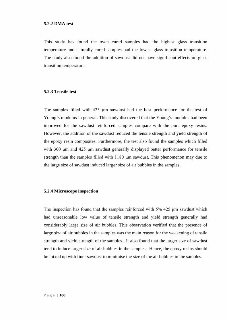
P a g e | 100

5.2.2 DMA test

This study has found the oven cured samples had the highest glass transition

temperature and naturally cured samples had the lowest glass transition temperature.

The study also found the addition of sawdust did not have significant effects on glass

transition temperature.

5.2.3 Tensile test

The samples filled with 425 μm sawdust had the best performance for the test of

Young’s modulus in general. This study discovered that the Young’s modulus had been

improved for the sawdust reinforced samples compare with the pure epoxy resins.

However, the addition of the sawdust reduced the tensile strength and yield strength of

the epoxy resin composites. Furthermore, the test also found the samples which filled

with 300 μm and 425 μm sawdust generally displayed better performance for tensile

strength than the samples filled with 1180 μm sawdust. This phenomenon may due to

the large size of sawdust induced larger size of air bubbles in the samples.

5.2.4 Microscope inspection

The inspection has found that the samples reinforced with 5% 425 μm sawdust which

had unreasonable low value of tensile strength and yield strength generally had

considerably large size of air bubbles. This observation verified that the presence of

large size of air bubbles in the samples was the main reason for the weakening of tensile

strength and yield strength of the samples. It also found that the larger size of sawdust

tend to induce larger size of air bubbles in the samples. Hence, the epoxy resins should

be mixed up with finer sawdust to minimise the size of the air bubbles in the samples.

P a g e | 101

5.2.5 Industrial applications

This report has found that oven cured epoxy resins have the lowest dielectric constant,

the lowest loss tangent, and the highest glass transition temperature. Hence, oven cured

epoxy resin is the best candidate for making PCBs. The loss tangents of the sawdust

reinforced epoxy resins were slightly higher than the loss tangents of pour epoxy resins.

Hence, the sawdust reinforced epoxy resin is slightly more efficient to be post-cured in

microwave than pure epoxy resin.

5.3 Further Research and Recommendations

The LCR meter used in the dielectric constant and loss tangent measurement can only

measure the dielectric constant and the loss tangent up to 100 kHz. However, most

frequencies of the microwaves used in both material processing industry and electronic

industry are above 2 GHz. Furthermore, the results obtained from the parallel plate

measurement method would contain inherent errors due to the air gap effect and the

edge effect. Hence, it is necessary to measure the dielectric constant and loss tangent

with better equipment to provide more accurate results for practical applications.

P a g e | 102

APPENDIX A A.1 – Project Specification

P a g e | 103

University of Southern Queensland

FACULTY OF ENGINEERING AND SURVEYING

ENG4111/4112 Research Project PROJECT SPECIFICATION

FOR: PING TAI

TOPIC: Tensile properties of sawdust reinforced epoxy composites post-cured in microwaves

SUPERVISOR: Dr. Harry Ku, and Dr. Francisco Cardona, USQ

ENROLMENT: ENG 4111 –S1,O,2010;

ENG 4111 –S2,O,2010

PROJECT AIM: The aim of this project is to produce a range of epoxy resin with different percentage by weight of sawdust as filler. The result of this project is to demonstrate the effect on tensile strength of the final product by adding different percentage of sawdust and the cost reduction by using cheaper filler such as sawdust.

SPONSORSHIP: None

PROGRAMME: Issue B, 27nd April 2010

11. Research the background information relating to epoxy resin, microwaves. 12. Produce six pieces of specimens with different percentage by weight of sawdust, post-cure the

specimens with microwaves. 13. Implement tensile test on the specimens 14. Carry out DMA test 15. Carry out the permittivity test 16. Analyse the test results. 17. Consider the material costs and the test results to recommend the best specimens for different

industrial applications. 18. Identify the possible defects on the specimens. 19. Suggest possible solution to minimise defects.

AGREED: _________________________ (Student) _____________________________ (Supervisor) Date: / /2010 Date:27 /04/2010 Examiner/Co-examiner:____________________________________Date: / /2010

P a g e | 104

APPENDIX B

B.1 High performance epoxy resins

P a g e | 105

P a g e | 106

P a g e | 107

P a g e | 108

P a g e | 109

APPENDIX C

C.1 Tensile test results

P a g e | 110

Report Date: 1/07/2010 Test Date : 1/07/2010 Method : MMT Tensile Test with return.msm 0% sawdust

Specimen Results:

Specimen #

Thickness

mm

Width

mm

Area

mm^2

Peak Load

N

Peak Stress

MPa

Break Load

N

Break Stress

MPa

1 7.260 25.530 185 8675 46.81 7543 40.70

2 7.820 25.000 196 9472 48.45 9472 48.45

3 7.700 25.050 193 8997 46.64 8997 46.64

4 7.470 25.100 187 8785 46.86 8752 46.68

Mean 7.562 25.170 190 8982 47.19 8691 45.62

Std Dev 0.249 0.243 5 353 0.85 822 3.39

Specimen #

Elongation At Break

mm

Stress At Offset Yield

MPa

Load At Offset Yield

N

Modulus

MPa

1 6.324 23.115 4284.249 2494

2 4.059 21.135 4131.840 2547

3 3.904 20.711 3994.873 2550

4 4.731 21.500 4031.129 2494

Mean 4.755 21.615 4110.523 2521

Std Dev 1.106 1.050 129.504 31

P a g e | 111

0

1000

2000

3000

4000

5000

6000

7000

8000

9000

10000

0 1 2 3 4 5 6 7

Load (N)

Extension (mm)

123[4]

P a g e | 112

5%300um sawdust

Report Date: 1/07/2010 Test Date : 1/07/2010 Method : MMT Tensile Test with return.msm

Specimen Results:

Specimen #

Thickness

mm

Width

mm

Area

mm^2

Peak Load

N

Peak Stress

MPa

Break Load

N

Break Stress

MPa

1 7.150 26.880 192 1286 6.69 1286 6.69

2 7.040 26.040 183 4964 27.08 4964 27.08

3 7.100 24.990 177 6805 38.35 6805 38.35

4 7.130 24.990 178 4980 27.95 4980 27.95

Mean 7.105 25.725 183 4509 25.02 4509 25.02

Std Dev 0.048 0.915 7 2316 13.25 2316 13.25

Specimen #

Elongation At Break

mm


MPa


N

Modulus

MPa

1 0.342 5.726 1100.436 3076

2 1.767 13.727 2516.434 2554

3 2.654 17.868 3170.385 2665

4 1.939 13.343 2377.453 2431

Mean 1.676 12.666 2291.177 2681

Std Dev 0.969 5.060 865.843 280

Modulus =2554+2665+2431/3 = 2550

Tensile = 27.08+38.35+27.05 = 30.83

P a g e | 113

0

1000

2000

3000

4000

5000

6000

7000

0.0 0.2 0.4 0.6 0.8 1.0 1.2 1.4 1.6 1.8 2.0 2.2 2.4 2.6 2.8

Load (N)

Extension (mm)

123[4]

P a g e | 114

5%-425um


Specimen Results:

Specimen #

Thickness

mm

Width

mm

Area

mm^2

Peak Load

N

Peak Stress

MPa

Break Load

N

Break Stress

MPa

1 8.470 24.990 212 2733 12.91 2733 12.91

2 8.870 25.080 222 2301 10.34 2290 10.29

3 8.720 24.800 216 2637 12.20 2637 12.20

4 8.800 24.800 218 1094 5.01 1094 5.01

Mean 8.715 24.917 217 2191 10.12 2189 10.10

Std Dev 0.174 0.141 4 754 3.57 754 3.57

Specimen #

Elongation At Break

mm


MPa


N

Modulus

MPa

1 0.717 9.564 2024.293 2845

2 0.626 9.136 2032.350 2737

3 0.655 9.733 2104.861 2893

4 0.270 4.702 1026.078 3031

Mean 0.567 8.284 1796.895 2877

Std Dev 0.201 2.401 515.154 122

Tensile = 12.91 +10.34 +12.2 /3 = 11.82

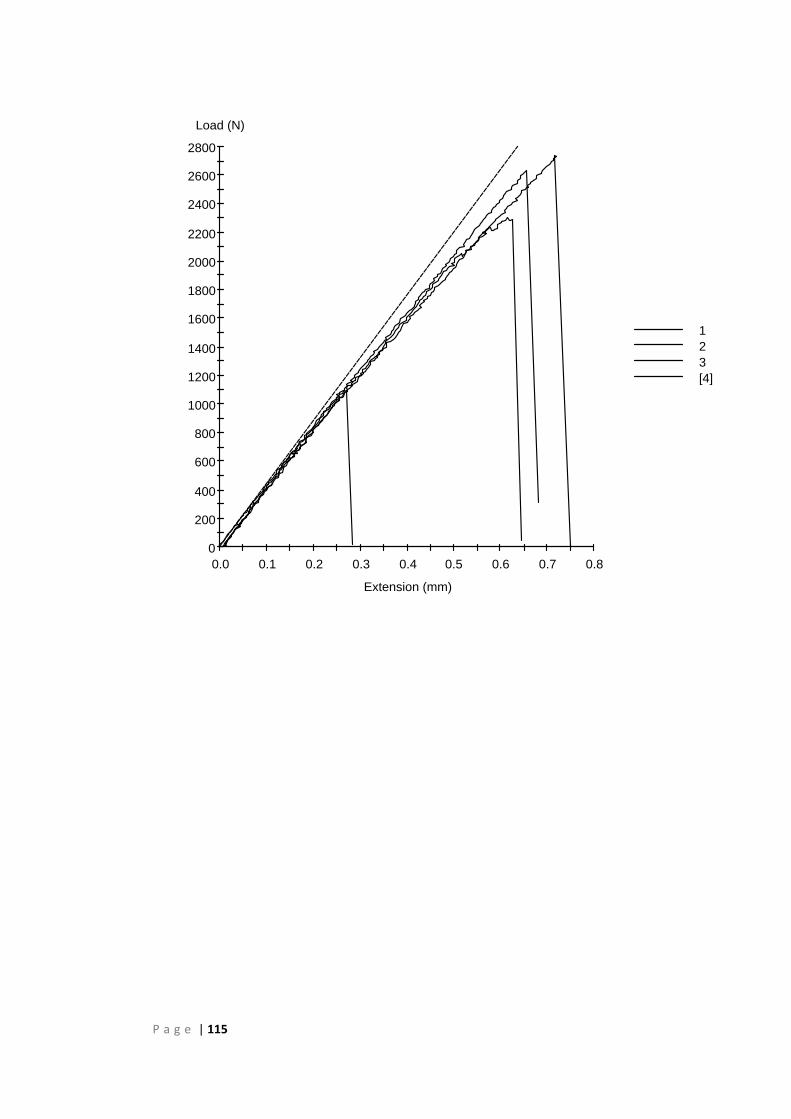
P a g e | 115

0

200

400

600

800

1000

1200

1400

1600

1800

2000

2200

2400

2600

2800

0.0 0.1 0.2 0.3 0.4 0.5 0.6 0.7 0.8

Load (N)

Extension (mm)

123[4]

P a g e | 116

5% 1180 um


Specimen Results:

Specimen #

Thickness

mm

Width

mm

Area

mm^2

Peak Load

N

Peak Stress

MPa

Break Load

N

Break Stress

MPa

1 7.790 23.870 186 2521 13.56 2521 13.56

2 7.200 24.930 179 2518 14.03 2518 14.03

3 6.910 25.140 174 3226 18.57 3226 18.57

4 6.980 25.000 174 4115 23.58 4115 23.58

Mean 7.220 24.735 178 3095 17.44 3095 17.44

Std Dev 0.400 0.583 6 757 4.68 757 4.68

Specimen #

Elongation At Break

mm


MPa


N

Modulus

MPa

1 0.819 9.857 1832.942 2615

2 0.819 9.463 1698.660 2732

3 1.167 8.831 1534.165 2655

4 1.524 11.370 1984.008 2591

Mean 1.082 9.880 1762.444 2648

Std Dev 0.337 1.079 191.694 61

Tensile = 18.57 + 23.58 = 21.075

P a g e | 117

0

1000

2000

3000

4000

5000

0.0 0.1 0.2 0.3 0.4 0.5 0.6 0.7 0.8 0.9 1.0 1.1 1.2 1.3 1.4 1.5 1.6

Load (N)

Extension (mm)

123[4]

P a g e | 118

10%300um


Specimen Results:

Specimen #

Thickness

mm

Width

mm

Area

mm^2

Peak Load

N

Peak Stress

MPa

Break Load

N

Break Stress

MPa

1 7.680 25.210 194 6157 31.80 6157 31.80

2 7.240 27.100 196 5668 28.89 5668 28.89

3 7.520 25.250 190 6842 36.03 6842 36.03

4 7.980 25.120 200 6211 30.98 6211 30.98

Mean 7.605 25.670 195 6219 31.93 6219 31.93

Std Dev 0.309 0.955 4 481 3.00 481 3.00

Specimen #

Elongation At Break

mm


MPa


N

Modulus

MPa

1 2.160 15.189 2940.763 2530

2 1.905 13.811 2709.799 2648

3 2.586 16.725 3175.756 2677

4 2.027 14.309 2868.251 2687

Mean 2.170 15.008 2923.643 2635

Std Dev 0.297 1.278 193.779 72

P a g e | 119

0

1000

2000

3000

4000

5000

6000

7000

0.0 0.2 0.4 0.6 0.8 1.0 1.2 1.4 1.6 1.8 2.0 2.2 2.4 2.6 2.8

Load (N)

Extension (mm)

123[4]

P a g e | 120

10% 425um


Specimen Results:

Specimen #

Thickness

mm

Width

mm

Area

mm^2

Peak Load

N

Peak Stress

MPa

Break Load

N

Break Stress

MPa

1 7.460 25.000 186 5831 31.26 5831 31.26

2 8.050 25.240 203 4013 19.75 4013 19.75

3 8.050 25.000 201 5730 28.47 5730 28.47

4 8.120 24.590 200 5788 28.99 5788 28.99

Mean 7.920 24.958 198 5340 27.12 5340 27.12

Std Dev 0.308 0.270 8 886 5.06 886 5.06

Specimen #

Elongation At Break

mm


MPa


N

Modulus

MPa

1 1.828 16.668 3108.615 2903

2 1.032 11.899 2417.569 3123

3 1.657 14.106 2838.878 2903

4 1.570 14.028 2800.943 3150

Mean 1.522 14.175 2791.501 3020

Std Dev 0.343 1.951 284.441 135

Tensile = 31.26+28.47+28.99 /3 = 29.57

P a g e | 121

0

1000

2000

3000

4000

5000

6000

0.0 0.2 0.4 0.6 0.8 1.0 1.2 1.4 1.6 1.8 2.0

Load (N)

Extension (mm)

123[4]

P a g e | 122

10%1180um


Specimen Results:

Specimen #

Thickness

mm

Width

mm

Area

mm^2

Peak Load

N

Peak Stress

MPa

Break Load

N

Break Stress

MPa

1 7.640 25.880 198 3057 15.46 3057 15.46

2 7.470 25.030 187 4415 23.61 4415 23.61

3 7.670 26.350 202 3374 16.69 3374 16.69

4 7.720 26.350 203 1312 6.45 1312 6.45

Mean 7.625 25.902 198 3039 15.55 3039 15.55

Std Dev 0.108 0.622 7 1289 7.05 1289 7.05

Specimen #

Elongation At Break

mm


MPa


N

Modulus

MPa

1 0.807 10.968 2168.645 3024

2 1.316 11.922 2229.072 2950

3 0.913 10.365 2094.790 2928

4 0.366 5.482 1115.207 2915

Mean 0.851 9.684 1901.929 2954

Std Dev 0.390 2.874 527.348 49

Tensile = 15.46 + 23.64 + 16.69 /3 = 18.59

P a g e | 123

0

1000

2000

3000

4000

5000

0.0 0.1 0.2 0.3 0.4 0.5 0.6 0.7 0.8 0.9 1.0 1.1 1.2 1.3 1.4

Load (N)

Extension (mm)

123[4]

P a g e | 124

15%-300um


Specimen Results:

Specimen #

Thickness

mm

Width

mm

Area

mm^2

Peak Load

N

Peak Stress

MPa

Break Load

N

Break Stress

MPa

1 7.000 25.060 175 5516 31.45 5516 31.45

2 7.240 24.970 181 5517 30.52 5517 30.52

3 7.060 25.060 177 4494 25.40 4494 25.40

4 6.800 25.580 174 4428 25.46 4428 25.46

Mean 7.025 25.168 177 4989 28.21 4989 28.21

Std Dev 0.181 0.278 3 610 3.23 610 3.23

Specimen #

Elongation At Break

mm


MPa


N

Modulus

MPa

1 1.924 15.344 2691.671 2904

2 1.909 13.435 2428.816 2853

3 1.350 16.527 2923.978 3039

4 1.324 11.568 2012.207 3218

Mean 1.627 14.219 2514.168 3004

Std Dev 0.335 2.178 391.025 163

P a g e | 125

0

1000

2000

3000

4000

5000

6000

0.0 0.2 0.4 0.6 0.8 1.0 1.2 1.4 1.6 1.8 2.0

Load (N)

Extension (mm)

123[4]

P a g e | 126

15%-425um


Specimen Results:

Specimen #

Thickness

mm

Width

mm

Area

mm^2

Peak Load

N

Peak Stress

MPa

Break Load

N

Break Stress

MPa

1 6.800 25.270 172 4658 27.11 4658 27.11

2 6.330 25.280 160 4717 29.47 4717 29.47

3 6.400 25.010 160 1561 9.75 1561 9.75

4 6.260 25.340 159 4756 29.98 4756 29.98

Mean 6.448 25.225 163 3923 24.08 3923 24.08

Std Dev 0.242 0.147 6 1575 9.63 1575 9.63

Specimen #

Elongation At Break

mm


MPa


N

Modulus

MPa

1 1.608 14.219 2443.251 2829

2 2.431 26.962 4314.463 1841

3 0.467 8.840 1414.991 3205

4 1.738 14.244 2259.453 2970

Mean 1.561 16.066 2608.039 2711

Std Dev 0.814 7.695 1222.554 600

Young’s = 2829+3205+2970/3 = 3001

Tensile = 27.11+29.47+29.98= 28.85

P a g e | 127

0

1000

2000

3000

4000

5000

0.0 0.2 0.4 0.6 0.8 1.0 1.2 1.4 1.6 1.8 2.0 2.2 2.4 2.6

Load (N)

Extension (mm)

123[4]

P a g e | 128

15%1180um


Specimen Results:

Specimen #

Thickness

mm

Width

mm

Area

mm^2

Peak Load

N

Peak Stress

MPa

Break Load

N

Break Stress

MPa

1 7.220 25.140 182 2518 13.87 2518 13.87

2 7.820 24.970 195 3399 17.41 3399 17.41

3 7.570 25.020 189 2222 11.73 2222 11.73

4 7.480 25.070 188 2484 13.25 2484 13.25

Mean 7.522 25.050 188 2656 14.06 2656 14.06

Std Dev 0.248 0.073 6 513 2.40 513 2.40

Specimen #

Elongation At Break

mm


MPa


N

Modulus

MPa

1 0.760 9.118 1655.019 2927

2 1.007 10.934 2135.075 2794

3 0.663 7.845 1485.824 2825

4 0.765 7.948 1490.524 2824

Mean 0.799 8.961 1691.610 2843

Std Dev 0.146 1.436 305.932 58

P a g e | 129

0

1000

2000

3000

4000

0.0 0.1 0.2 0.3 0.4 0.5 0.6 0.7 0.8 0.9 1.0 1.1

Load (N)

Extension (mm)

123[4]

P a g e | 130

16.7% 300 um


Specimen Results:

Specimen #

Thickness

mm

Width

mm

Area

mm^2

Peak Load

N

Peak Stress

MPa

Break Load

N

Break Stress

MPa

1 8.150 24.990 204 6390 31.37 6390 31.37

2 7.870 25.290 199 5835 29.31 5835 29.31

3 7.560 25.200 191 1880 9.87 1880 9.87

4 7.530 25.150 189 5519 29.14 5519 29.14

Mean 7.778 25.158 196 4906 24.92 4906 24.92

Std Dev 0.292 0.126 7 2049 10.09 2049 10.09

Specimen #

Elongation At Break

mm


MPa


N

Modulus

MPa

1 1.888 14.660 2985.748 2985

2 1.667 14.573 2900.479 3002

3 0.538 8.476 1614.734 2995

4 1.628 17.521 3318.094 2994

Mean 1.430 13.807 2704.764 2994

Std Dev 0.606 3.809 748.687 7

Tensile = 31.37 + 29.31 +29.14 /3 = 29.94

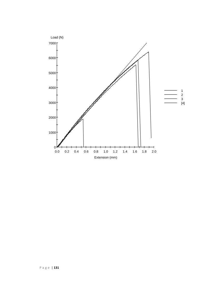
P a g e | 131

0

1000

2000

3000

4000

5000

6000

7000

0.0 0.2 0.4 0.6 0.8 1.0 1.2 1.4 1.6 1.8 2.0

Load (N)

Extension (mm)

123[4]

P a g e | 132

16.7% - 425um


Specimen Results:

Specimen #

Thickness

mm

Width

mm

Area

mm^2

Peak Load

N

Peak Stress

MPa

Break Load

N

Break Stress

MPa

1 7.210 25.040 181 5334 29.55 5334 29.55

2 7.080 25.210 178 4717 26.43 4717 26.43

3 7.160 24.690 177 5126 29.00 5126 29.00

4 7.170 25.040 180 4239 23.61 4239 23.61

Mean 7.155 24.995 179 4854 27.15 4854 27.15

Std Dev 0.054 0.219 2 484 2.72 484 2.72

Specimen #

Elongation At Break

mm


MPa


N

Modulus

MPa

1 1.524 13.927 2514.420 3250

2 1.382 12.244 2185.430 3242

3 1.496 13.980 2471.450 3258

4 1.187 14.095 2530.534 3229

Mean 1.397 13.562 2425.458 3245

Std Dev 0.153 0.881 161.950 12

Tensile = 29.55 + 26.43 + 29.00 = 28.32

P a g e | 133

0

1000

2000

3000

4000

5000

6000

0.0 0.1 0.2 0.3 0.4 0.5 0.6 0.7 0.8 0.9 1.0 1.1 1.2 1.3 1.4 1.5 1.6

Load (N)

Extension (mm)

123[4]

P a g e | 134

16.7%1180um


Specimen Results:

Specimen #

Thickness

mm

Width

mm

Area

mm^2

Peak Load

N

Peak Stress

MPa

Break Load

N

Break Stress

MPa

1 8.980 25.110 225 2950 13.08 2950 13.08

2 9.660 25.220 244 2735 11.23 2735 11.23

3 8.800 25.000 220 1222 5.55 1222 5.55

4 8.950 25.120 225 1900 8.45 1900 8.45

Mean 9.098 25.112 228 2202 9.58 2202 9.58

Std Dev 0.383 0.090 10 795 3.29 795 3.29

Specimen #

Elongation At Break

mm


MPa


N

Modulus

MPa

1 0.940 9.213 2077.334 2248

2 0.848 8.075 1967.223 2116

3 0.389 4.796 1055.116 2236

4 0.598 7.606 1710.074 2207

Mean 0.693 7.422 1702.437 2202

Std Dev 0.249 1.876 458.164 60

Tensile = 13.08 + 11.23 /2 = 12.155

P a g e | 135

0

1000

2000

3000

0.0 0.1 0.2 0.3 0.4 0.5 0.6 0.7 0.8 0.9 1.0

Load (N)

Extension (mm)

123[4]

P a g e | 136

References Australian/New Zealand Standard 2002, Household and similar electrical appliances—Safety Part 2.25: Particular requirements for microwave ovens including combination microwave ovens (IEC 60335-2-25: Ed 5.2, IDT), Standards Australia/Standards New Zealand, Sydney, NSW, viewed 3 May, 2010. <http://www.saiglobal.com.ezproxy.usq.edu.au/online/Script/OpenDoc.asp?name=AS%2FNZS+60335%2E2%2E25%3A2002&path=http%3A%2F%2Fwww%2Esaiglobal%2Ecom%2FPDFTemp%2Fosu%2D2010%2D05%2D03%2F7852623125%2F60335%2E2%2E25%2D2002%28%2BA4%29%2Epdf&docn=AS592021179976 >. California Department of Public Health 1989, Epoxy resin systems, California Department of Public Health, California, United States, viewed 3 May 2010, <http://www.cdph.ca.gov/programs/hesis/Documents/epoxy.pdf>.

Carl Hanser Verlag GmbH & Co. KG, 2006, Dynamic Mechanical Analysis, Hanser Publishers Ltd.

<http://files.hanser.de/hanser/docs/20041012_2411215439-82_3-446-22673-7.pdf>

Harper, CA 1992, Handbook of plastics, elastomers, and composites, 2nd edn, McGraw-Hill, Inc , New York, United States.

Ku, HS, Wong, P, Huang, J, Fung, H, and Trada, M 2000, Tensile tests of glass powder reinforced epoxy composites post-cured in microwaves: pilot study. Journal of Compsites, Australia.

Ku, HS, Ball, JAR, Siores, E & Chan, P 1999, Complex permittivity of low loss thermoplastic composites using a resonant cavity method. ICCM-12: 12th International Conference on Composite Materials, Paris, France. Ku, HS, Siores, E, Ball, JAR and Horsfiled, B 1998, An Important Step in Microwave Processing of Materials: Permittivity Measurements of thermoplastic Composites at Elevated Temperatures, Proceedings of 1998 Pacific Conference on Manufacturing, Brisbane, Australia, August 18 - 21, (1998) pp. 68-73.

Ku, H, Prajapati, M and Cardona, F 2010, Thermal properties of sawdust reinforced vinyl ester composites post-cured in microwaves: pilot study, Australia.

Ku, H, Prajapati, M and Cardona, F 2010a, Thermal properties of sawdust reinforced vinyl ester composites post-cured in microwaves: pilot study, Australia.

P a g e | 137

Ku, H, Prajapati, M and Cardona, F 2010b, Thermal properties of calcium carbonate powder reinforced vinyl ester composites: pilot study, Australia.

Lin, SC 1994, High-performance thermosets: chemistry, properties, applications, Hanser Publishers, New York, USA

Morin, B 2007, PCB fabrication – low dielectric fabrics, OnBorad Technology Ltd, viewed 23 July 2010,

<http://www.onboard-technology.com>

Meredith, R 1998, Engineers’ handbook of industrial microwave heating, The Institution of Electrical Engineers, London, United Kingdom.

National Research Council (U.S.) 1994, Microwave processing of materials, National Academy Press, Washington DC, U.S.

Pritchard, G 1999, Reinforced plastics durability, Woodhead Publishing Ltd, England

Platts, J 1991, Microwave ovens, Peter Peregrinus Ltd, London, United Kingdom.

Sadiku, MN 2001, Elements of electromagnetic s, 3rd edn, Oxford University Press, New York.

Thuery, J 1992, Microwaves: Industrial, Scientific and Medical Applications, Artech House, Norwood, MA.

University of Southern Queensland 2009, ELE4605 Fields and waves, USQ, Toowoomba, Queensland, Australia.