project vt/2007/017 an investigation into occupational
TRANSCRIPT
Project VT/2007/017
An Investigation into Occupational Exposure to Electromagnetic Fields for Personnel Working With and Around Medical Magnetic Resonance Imaging Equipment
04 April 2008
The statements and recommendations of this report do not necessarily reflect the position of the European Commission.
2

3
Project VT/2007/017
An Investigation into Occupational Exposure to Electromagnetic Fields for Personnel Working with and around Medical Magnetic Resonance Imaging Equipment
Myles Capstick, Donald McRobbie, Jeff Hand, Andreas Christ, Sven Kühn, Kjell Hansson Mild, Eugenia Cabot, Yan Li, Amir Melzer, Annie Papadaki, Klaas Prüssmann,
Rebecca Quest, Marc Rea, Salome Ryf, Michael Oberle, Niels Kuster
Contractors:
Foundation for Research on Information Technology in Society - IT'IS (Principle)
Imperial College London
Subcontractors:
Imperial College Health Care NHS Trust (Radiological Sciences Unit) London
Umeå University, Department of Radiation Physics
MR Center, University Hospital Zurich
04 April 2008
for the
EUROPEAN COMMISSION
Employment, Social Affairs and Equal Opportunities DG
The statements and recommendations of this report do not necessarily reflect the position of the European Commission.

4
5
Executive Summary
Magnetic Resonance Imaging (MRI) is a rapidly developing diagnostic technology that provides an unmatched view inside the human body without applying ionizing radiation. Improved image quality and novel applications, however, generally require higher electromagnetic field (EMF) strengths and faster image acquisitions, both of which may result in an increase in the EMF exposure of patients and workers. Over the past 30 years, safety standards limiting human exposure to EMFs were developed by agencies (e.g., FDA [1] and NRPB [2]-[5]) and product standard organizations [6] to specifically address the safety of patients undergoing MRI scans as well as by standard bodies like ICNIRP [9]-[12] and ICES [7],[8] to establish safety limits covering the entire spectrum from DC to light. The MRI exposure guidelines are mainly based on specific research results on nerve stimulation by induced low frequency currents, whereas the latter standards are based on biological experiments conducted at different frequencies and conditions and that have been extrapolated to the entire spectrum including the MR relevant frequencies. Inconsistencies inevitably resulted, although no attempt was ever made to resolve them with targeted research projects.
When the EU decided to enforce the ICNIRP guidelines for occupational exposures to electromagnetic fields (EU Directive 2004/40/EC [13]), MRI experts claimed that the directive would unnecessarily restrict current and future developments in the field of MRI technology and the medical procedures and interventions carried out using MRI equipment. This study aimed to fill gaps in knowledge about actual exposures during routine MRI procedures.
Potential short-term hazards are, for example, nerve stimulation resulting from induced currents caused by gradient fields and movements in the static fields as well as thermal tissue damage from the exposure to radio frequency (RF) electromagnetic fields. Workers exposed occupationally include radiologists, interventionalists, nurses, researchers, technicians and other personnel such as cleaners.
The overall project objectives were addressed based on the following subtasks:
• Gaining a comprehensive understanding of existing and future medical procedures and technologies.
• Identifying possible worst-case scenarios with respect to pulse sequences, phase coding, field gradients, etc.
• Developing appropriate instrumentations and systematically measuring the strength of the fields during pre-selected procedures.
• Applying experimentally validated numerical models to assess if the measured incident fields exceed the physical limits set out in Directive 2004/40/EC.
• Extrapolation of the findings to any scanner and all procedures by uncertainty evaluations
• Examining protocols and medical practices used in and assessing possible changes to eliminate or reduce exposure.
The European Society of Radiology preselected four sites with 1.0 T, 1.5 T, 3.0 T and 7.0 T machines representing the current state of the art in MRI technology and practice. Time and cost considerations limited the project to just these four sites and considerably increased the uncertainty with respect to general conclusions. The results obtained by applying the most advanced tools (instrumentation, simulation tools, human models) were extrapolated to derive firm conclusions regarding worker's exposure and requirements for future studies. The majority of the investigated procedures were well within the limits of Directive 2004/40/EC except for interventional MR applications, close personnel attendance during scans and fast movements in the static field while cleaning the machines.

6
Within the limitations and uncertainties, the conclusions of this study are as follows.
RF exposure:
• The basic restrictions regarding RF exposures for workers based on 2004/40/EC can be met for any of the current procedures except when two persons are simultaneously inside a cylindrical bore system. Any body overlap should be avoided as it can lead to much higher exposures that considerably exceed the guidelines.
• Currently applied procedures for interventional MRI applications result in SAR values close to the SAR limits. However, the exposure could be minimized with appropriate measures (see below).
Induced Currents by Gradients and Movements:
• The basic restrictions regarding induced currents in the CNS based on the ICNIRP guidelines [9] determined according to [6] are violated for persons positioned next to the scanners by a factor of up to 10 and even more for movements.
• In the case of interventional MRI, the induced currents may exceed a factor of 50 compared to current guidelines.
• The prevalent cleaning procedures require the personnel to crawl inside the scanners, possibly leading to considerable induced currents.
Acoustic Noise Exposure: The maximum measured acoustic noise value for the tested sequences was below 110 dB(A). All scanners exceeded the recommended threshold of 80 dB(A) for using hearing protectors [Directive 2003/10/EC [14]].
Various possibilities ranging from general exclusions for MR operations to limiting MR usage have been suggested to avoid conflict with the planned directive. Without a compromise, advancements in MR technology for beneficial medical applications might be limited. Based on our knowledge of the basis of the safety limits and dosimetry, we recommend the following measures to avoid the potential disadvantages and to foster the development of MR technology for future applications.
• Immediate initiation of targeted research to fill the knowledge gaps regarding potential hazards for these specific exposures. This will empower the standard bodies to revisit the standard and to introduce conservative limits without including extra margins for unknowns.
• Detailed and accurate information about the exposure anywhere inside the bore as well as in the vicinity of the scanner could be made available instantly (e.g., as an MR software feature). The effort/cost would be comparably small for MR manufacturers (<0.1% per device) since each coil design will require only one evaluation from which all current and future applications can be derived. This would have the benefit that any unnecessary peak exposure for patients and workers during specific MR applications could be eliminated by intelligent software control.
• Training of personnel to understand when and where peak exposures occur and how to minimize the exposure.
• Develop standard evaluation procedures as well as improved evaluation techniques including measurement instruments for incident field assessments and numerical tools for the dosimetric evaluations.
The authors of this report are convinced that the recommendations can be implemented within three years such that current and future MR applications are not restricted by the EU directive for workers. In the long term, the enforcement of defined and improved guidelines combined with standardized compliance procedures will result in accelerated developments of MR technology.

7
Contents
1 Objectives.......................................................................................................................17 2 Review of Standards Framework ...................................................................................19
2.1 Introduction.............................................................................................................19 2.2 Time-varying EM fields ...........................................................................................19 2.3 Static Fields ............................................................................................................22 2.4 Other Guidance and Standards..............................................................................23
2.4.1 Patients...........................................................................................................23 2.4.2 Other Occupational Limits ..............................................................................25
2.5 Acoustic Noise........................................................................................................25 3 Status Quo and Developments in Clinical MRI...............................................................27
3.1 Introduction.............................................................................................................27 3.2 Electromagnetic Field Exposures in MRI................................................................27
3.2.1 Static Field Exposure......................................................................................27 3.2.2 EMF Exposure from the Imaging Gradients ...................................................27 3.2.3 Radiofrequency Exposures.............................................................................28
3.3 Future Trends in MRI Applications .........................................................................28 3.4 Other Areas of MR Potentially Affected by Directive 2004/40/EC ..........................30
4 Observation of Clinical Procedures - Method .................................................................31 4.1 Participating Centres ..............................................................................................31 4.2 Sites and MRI Machines.........................................................................................32
4.2.1 Philips 1.0 T Panorama ..................................................................................32 4.2.2 Siemens 1.5 T Avanto ....................................................................................34 4.2.3 Philips 3.0 T Achieva ......................................................................................36 4.2.4 Philips 7.0 T Intera..........................................................................................38
4.3 Initial Visits..............................................................................................................39 4.4 Video Visits.............................................................................................................39
4.4.1 Video Recording System ................................................................................39 4.4.2 Method on Site................................................................................................39
4.5 Analysis of Videos ..................................................................................................41 4.6 Additional Tasks .....................................................................................................41 4.7 Initial Selection of Procedures ................................................................................41 4.8 Sequences..............................................................................................................42
4.8.1 Balanced-FFE/TrueFISP ................................................................................44 4.8.2 Echo-Planar Imaging ......................................................................................44
8
4.8.3 Diffusion-Weighted / Diffusion Tensor Imaging ..............................................45 4.8.4 T2-Weighted Turbo Spin Echo .......................................................................45
4.9 Other Physical Agents and Measurements ............................................................46 4.9.1 Acoustic Noise ................................................................................................46 4.9.2 Temperature and Humidity .............................................................................46 4.9.3 Bio-Effects Staff Questionnaire.......................................................................46
5 Observation of Clinical Procedures - Results and Analysis............................................47 5.1 Cologne 1.0 T .........................................................................................................48 5.2 Procedures .............................................................................................................48 5.3 Strasbourg 1.5 T.....................................................................................................54
5.3.1 Procedures .....................................................................................................55 5.3.2 Acoustic Noise ................................................................................................58
5.4 Leuven 3.0T / 1.5 T ................................................................................................59 5.4.1 Procedures .....................................................................................................60 5.4.2 Acoustic Noise ................................................................................................64
5.5 Nottingham 7.0 T ....................................................................................................65 5.5.1 Procedures .....................................................................................................66 5.5.2 Acoustic Noise ................................................................................................68 5.5.3 Temperature and Humidity .............................................................................69
5.6 Bio-Effects Questionnaire .......................................................................................69 5.7 Consultation with Radiological and Clinical Experts ...............................................70
6 Assessment of Incident Fields........................................................................................71 6.1 Methods..................................................................................................................71
6.1.1 Background.....................................................................................................71 6.1.2 Overview.........................................................................................................71
6.2 Instrumentation.......................................................................................................72 6.2.1 B-field..............................................................................................................72 6.2.2 Gradient Field .................................................................................................72 6.2.3 RF Field ..........................................................................................................74 6.2.4 Data Acquisition Software System..................................................................75 6.2.5 Measurements ................................................................................................78
6.3 Measurement Procedure ........................................................................................79 6.3.1 Measurement Preparation ..............................................................................79 6.3.2 Measurement Procedure ................................................................................82 6.3.3 Clinical Sequence Measurement ....................................................................85
6.4 Static Field Measurements .....................................................................................87 6.4.1 Philips 1.0 T ....................................................................................................87 6.4.2 Siemens 1.5 T.................................................................................................90

9
6.4.3 Philips 3.0 T Achieva ......................................................................................92 6.4.4 Philips 7.0 T Intera..........................................................................................95
6.5 Static Field Gradients .............................................................................................98 6.5.1 Siemens 1.5 T Avanto. ...................................................................................98 6.5.2 Philips 3.0 T Achieva ....................................................................................101 6.5.3 Philips 7.0 T Intera........................................................................................103
6.6 Gradient Field Measurements ..............................................................................107 6.6.1 Clinical Sequences Philips Panorama 1.0 T.................................................109 6.6.2 Gradient Test Sequence for Siemens 1.5 T Avanto .....................................117 6.6.3 Clinical Sequence Gradient Fields Siemens 1.5T ........................................118 6.6.4 Gradient Fields from the Test Sequence for the Philips 3.0 T Achieva ........125 6.6.5 Clinical Sequence Gradient Fields Philips 3.0 T Achieva .............................126 6.6.6 Clinical Sequences Philips 7.0 T Intera ........................................................138
6.7 RF Field Measurements .......................................................................................144 6.7.1 Philips 1.0 T Panorama ................................................................................144 6.7.2 Siemens 1.5 T Avanto ..................................................................................147 6.7.3 Philips 3.0 T Achieva ....................................................................................152 6.7.4 Philips 7.0T Intera.........................................................................................157
6.8 Summary of Results .............................................................................................158 6.8.1 Action Values................................................................................................158 6.8.2 Measurement Summary Outside the Bore ...................................................158 6.8.3 Measurement Summary Inside the Bore ......................................................159
6.9 Conclusions ..........................................................................................................160 7 Assessment of Induced Fields......................................................................................163
7.1 Introduction...........................................................................................................163 7.2 Objectives.............................................................................................................163 7.3 Present State of Research ...................................................................................164
7.3.1 SAR Induced by RF Electromagnetic Fields.................................................164 7.3.2 Currents due to Time Varying Gradient Fields .............................................164 7.3.3 Currents due to Movements in Static Fields .................................................164
7.4 Numerical Methods...............................................................................................165 7.4.1 RF Simulations using FDTD and FIT............................................................165 7.4.2 Low Frequency Magnetic Fields ...................................................................165 7.4.3 Movements through Static Fields .................................................................166
7.5 Anatomical Models ...............................................................................................167 7.5.1 The Virtual Family – CAD Models of the Human Body.................................167 7.5.2 TIM Voxel Model...........................................................................................169
7.6 MR Scanner Models and Validation .....................................................................172

10
7.6.1 Philips 3.0 T Achieva ....................................................................................172 7.6.2 Siemens 1.5T Avanto ...................................................................................176 7.6.3 Philips 1.0 T Panorama ................................................................................179 7.6.4 Generic Solenoid ..........................................................................................187
7.7 RF Field Exposure................................................................................................187 7.7.1 Siemens 1.5T Avanto: Carer Accompanying Child.......................................187 7.7.2 Siemens 1.5T Avanto: Head Exposure to RF Coil........................................188 7.7.3 Siemens 1.5 T Avanto: Bystander Exposure ................................................190 7.7.4 Philips 1.0 T Panorama: Radiologist Exposure ............................................192 7.7.5 Normalization to Measurement Results........................................................193
7.8 Gradient Field Exposure.......................................................................................194 7.8.1 Philips 3.0 T Achieva: Bystander Exposure..................................................194 7.8.2 Siemens 1.5T Avanto: Head Exposure to Gradient Coil...............................199 7.8.3 Siemens 1.5T Avanto: Exposure of Carer to Gradient Coil ..........................201 7.8.4 Philips 1T Panorama: Radiologist Exposure ................................................201 7.8.5 Normalization to Measurement Results........................................................203
7.9 Static Field Exposure............................................................................................204 7.9.1 Generic Model: Bystander Exposure ............................................................204 7.9.2 Normalization to Measurement Results........................................................205
7.10 Summary and Requirements ................................................................................206 8 Uncertainty Assessment...............................................................................................207
8.1 Introduction...........................................................................................................207 8.2 Concept of Uncertainty Assessment.....................................................................207 8.3 Offset and Uncertainty of Static Magnetic Field Evaluation..................................209 8.4 Offset and Uncertainty of Gradient Field Evaluation.............................................210 8.5 Offset & Uncertainty of Incident RF H-Field Evaluation........................................211 8.6 Offset / Uncertainty of Incident RF E-Field Evaluation (Outside Bore) .................212 8.7 Offset and Uncertainty of Peak Spatial SAR Values ............................................213 8.8 Offset and Uncertainty of Induced Currents by Gradient Fields ...........................214 8.9 Offset and Uncertainty of Induced Currents by Static Fields ................................215
9 Conclusions..................................................................................................................217 9.1 Overview...............................................................................................................217 9.2 Site Evaluations....................................................................................................217
9.2.1 Cologne 1.0 T Panorama clinical procedures analysis .................................218 9.2.2 Strasbourg 1.5 T Avanto clinical procedure analysis ....................................220 9.2.3 Leuven 3.0 T Achieva clinical sequence analysis.........................................221 9.2.4 Nottingham 7.0 T Intera clinical procedure analysis .....................................222 9.2.5 Measurement Summary ...............................................................................223

11
9.3 Conclusions Based on Observed Clinical Practice...............................................224 9.3.1 Cologne 1.0 T Panorama..............................................................................224 9.3.2 Strasbourg 1.5 T Mid-Field System ..............................................................225 9.3.3 Leuven 3.0 T High Field System...................................................................225 9.3.4 Nottingham 7.0 T Ultra-High Field System ...................................................225
9.4 Worst Case Evaluations .......................................................................................225 9.5 Recommendations................................................................................................227
10 References ...............................................................................................................217

12
13
Abbreviations
ACR American College of Radiology
AV Action Value
BAMRR British Association of Magnetic Resonance Radiographers
b-FFE Balanced Fast Field Echo
BGV Berufsgenossenschaft Vorschriften
b-TFE Balanced Turbo Field Echo
CAD Computer Aided Design
CISS Constructive Interference Steady State
CNS Central Nervous System Tissue
dB DeciBell - The ratio of X/Xref are given in dB, i.e., dB(X/Xref) = A log10 (X/Xref) whereby A is 10 for SAR and 20 for field values (E, H, j)
DICOM Digital Imaging and Communications in Medicine Standard
DTI Diffusion Tensor Imaging
DW-EPI Diffusion Weighted – Echo Planar Imaging
DW-SSh Diffusion Weighted single shot echo
DW-SSh-org
Diffusion Weighted single shot echo planar imaging
DWI Diffusion Weighted Imaging
EEG Electroencephalogram
ELF Extremely low frequency
ELV Exposure Limit Value
EM Electromagnetic
EMF Electromagnetic Fields
EN European Norm
EPI Echo Planar Imaging
ESR European Society of Radiology
ETHZ Eidgenössische Technische Hochschule Zürich
FDA U.S. Food & Drug Administration
FDTD Finite Difference Time Domain
FE-EPI Field Echo – Echo Planar Imaging
FEM Finite Element Modelling
FFE Fast Field Echo
FIT Finite Integration Technique
FLAIR Fluid Attenuation Inversion Recovery
fMRI Functional Magnetic Resonance Imaging
FOV Field of View
14
FS Frequency Scaling
GA General Anaesthesia
GE-EPI Gradient Echo – Echo Planar Imaging
Gfe Frequency Encode Gradient
Gpe Phase Encode Gradient
Gss Slice Select Gradient
HASTE Half Fourier Acquisition Single Shot Turbo Spin Echo
HFO High Field Open (Philips Panorama MRI system)
HPA Health Protection Agency
IB Inside bore
ICES IEEE International Committee on Electromagnetic Safety
iCMR Interventional Cardiovascular Magnetic Resonance Imaging
ICNIRP International Commission on Non-Ionizing Radiation Protection
IEC International Electrotechnical Commission
IEEE Institute of Electrical and Electronics Engineers
iMR Interventional Magnetic Resonance
IT’IS The Foundation for Research on Information Technologies in Society
LAeq A-weighted RMS Sound Pressure Level averaged over the measurement period
LAFmax Maximum Sound Pressure Level during the measurement period
LHS Left Hand Side
MDA Medical Devices Agency (U.K.)
MGE Maxwell Grid Equation
MHRA Medicines and Healthcare Products Regulatory Agency
MP-RAGE Magnetisation Prepared Rapid Acquisition Gradient Echo
MRI Magnetic Resonance Imaging
MRS Magnetic Resonance Spectroscopy
NRPB National Radiological Protection Board
OB Out of bore
PAD Physical Agents Directive
PCI Peripheral Component Interconnect
PNS Peripheral Nerve Stimulation
psSAR Peak Spatial Specific Absorption Ratio
PXI PCI eXtensions for Instrumentation
RF Radio Frequency
RHS Right Hand Side
RMS Root Mean Square
RSS Root Sum Square
15
S Siemens, measure of electrical conductivity
SAR Specific Absorption Ratio (W/kg)
sBTFE Realtime Balanced Turbo Field Echo
SNR Signal to Noise Ratio
SPEAG Schmid & Partner Engineering AG
SPL Sound Pressure Level
SQ-engine Siemens gradients strength of 45 mT/m @ 200 T/m/s
SSFP Steady State Free Precession
SS-TSE Single Shot – Turbo Spin Echo
T1w-SE T1-weighted spin echo
T2-TSE T2-weighted turbo spin echo
TE Echo Time
TFE Turbo Field Echo
TIM Tomographic Image Model
TMS Transcranial magnetic stimulation
TR Repetition Time
TrueFISP True Fast Imaging with Steady state Precession
TSE Turbo Spin Echo
USZ University Hospital Zurich
wbSAR Whole-body Specific Absorption Ratio
WHO World Health Organization (U.N.)

17
1 Objectives
Magnetic Resonance Imaging (MRI) is a rapidly developing diagnostic technology that provides an unmatched view inside the human body without applying ionizing radiation. Improved image quality and novel applications, however, generally require higher electromagnetic field (EMF) strengths and faster image acquisitions, both of which result in an increase in the EMF exposure of patients and workers.
Over the past 30 years safety standards limiting human exposure to EMFs were developed by agencies (e.g., FDA [1] and NRPB [2]-[5]) and product standard organizations [6] to specifically address the safety of patients undergoing MRI scans as well as by standard bodies like ICNIRP [9]-[12] and ICES [7],[8] to establish safety limits covering the entire spectrum from DC to light. The MRI exposure guidelines are mainly based on specific research results on nerve stimulation by induced low frequency currents, these are also supported by anecdotal evidence based on millions of scans, whereas the latter standards are based on biological experiments conducted at different frequencies and conditions and that have been extrapolated to the entire spectrum including the MR relevant frequencies. Inconsistencies inevitably resulted, although no attempt was ever made to resolve them with targeted research projects. For example, occupational exposures have never been systematically investigated. Conflict further erupted when the EU decided to enforce the ICNIRP guidelines for occupational exposures (EU Directive 2004/40/EC [13]) to this unresolved situation. Experts claim that the directive will unnecessarily restrict current and future developments in the field of MRI technology and medical procedures and interventions carried out using MRI equipment.
This study aimed to fill gaps in knowledge about actual exposures and the potential hazards of MR workers during routine MRI procedures by applying the state-of-the art experimental and numerical tools and to identify future needs while avoiding potential hazards without restricting the medical explorations of the MR technology.
Potential short-term hazards are nerve stimulation resulting from induced currents caused by movements in the static fields and by the gradient fields as well as thermal tissue damage from the exposure to radio frequency (RF) electromagnetic fields. Workers risking occupational exposure include radiologists, interventionalists, nurses, researchers, technicians and other personnel such as cleaners.
The overall project objectives were achieved based on the following subtasks:
• Gaining a comprehensive understanding of existing medical procedures as well as those, which might be implemented from research into clinical practice in the near future.
• Referencing identified procedures to existing or upcoming MR technology, along with analysis and prioritisation in consultations with clinical experts and MRI technology suppliers; identification of possible worst-case scenarios with respect to pulse sequences, phase coding, field gradients, etc.
• Systematically measure the strength of the fields during pre-selected procedures with regard to movements of personnel in designated medical MRI installations; the results have been compared with the existing action values of Directive 2004/40/EC.
• Apply experimentally validated numerical models of gradient and RF coils to verify if the identified situations represent a possible worst-case scenario and calculate the corresponding exposures in terms of current density and SAR, especially if the measured incident field values exceeded the action values.
• Evaluate the findings from the modelling versus the measurements and determine the uncertainty of the simulation and measurement results.

18
• Examine protocols and medical practices used in the selected installations and assess possible changes to eliminate or reduce exposure and their feasibility.
• Identify the need for improved tools that identify hazards with minimal uncertainties.
The results will be interpreted and compared to the findings of the existing regulations. The closed and remaining open issues will be characterized and recommendations for modifying existing clinical practices or the underlying regulations, if necessary, will be offered.

2 Review of Standards Framework
2.1 Introduction
Guidelines and safety standards relating to MRI have been in existence for many years (e.g. NRPB 1984 [2], 1991 [4]; MDA 2002 [19], FDA 2003 [1]). These guidelines primarily consist of advice on the appropriate exposure limits for patients and practical safety issues. In the European Union, MR equipment is manufactured according to the IEC 60601-2-33 standard [6] which defines EMF exposure limits for patients and workers and the measurement methods required to demonstrate compliance. The limits defined in IEC 60601-2-33 are generally incorporated into the control software of the MR equipment, making it impossible under normal operation to exceed these limits. The IEC 60601-2-33 standard second amendment (Nov. 2007) defines EMF exposure limits for "MR-workers". It should be noted however that the IEC limits do not necessarily conform to other guidance, for example, from the Health Protection Agency (HPA, formally NRPB), and ICNIRP or from the mandatory provisions of Directive 2004/40/EC of the European Parliament and of the Council of 29 April 2004 [13].
Directive 2004/40/EC refers to the minimum health and safety requirements regarding the exposure of workers to the risks arising from physical agents (electromagnetic fields) and unlike guidelines and standards sets legally enforceable minimum requirements for limits on the acute occupational exposure of workers to electromagnetic fields, owing to their effects on the health and safety of workers. Specifically it only addresses risks resulting from “known short term adverse effects in the human body caused by the circulation of induced currents and by energy absorption as well as by contact currents.” In the case of exposure to fields associated with magnetic resonance imaging (MRI) systems, these limits are as described in Table 1. The corresponding action values, based on directly measurable parameters and for which compliance ensures compliance with the relevant exposure limit, are listed in Table 2. Directive 2004/40/EC does not address longer term effects, such as carcinogenesis.
This section reviews the range of current standards, their scope and summarises the reasoning behind the limits for each. It is not intended as a review of the literature of biological effects of EM fields, but only of the standards themselves and the publications wherein they are defined. For a detailed current review of the biological effects of electromagnetic (EM) fields see WHO (2007) [15] and Barnes and Greenbaum (2007) [16].
2.2 Time-varying EM fields
The limits upon which the Directive 2004/40/EC is based originate from ICNIRP guidelines [10] for time-varying electric, magnetic and electro-magnetic fields using the ICNIRP reference values as action values (AVs) and the Basic Restrictions as exposure limit values (ELVs). ICNIRP 1998 provides a review of the scientific evidence underpinning the limits. As the basis of the Directive 2004/40/EC limits, ICNIRP 1998 [10] provides “guidelines for limiting EMF exposure that will provide protection against known adverse health effects.” It further states that “an adverse health effect causes detectible impairment of the health of the exposed individual or of his or her offspring.” The basic restrictions are defined in terms of induced current density J (A/m2) in tissue for frequencies up to 10 MHz and Specific Absorption Rate SAR (W/kg) for frequencies from 100 kHz to 300 GHz based directly upon “established health effects”. These limits are not necessarily directly measurable. For practical exposure assessment, Reference Levels are defined in terms of electric and magnetic field quantities E (electric field), H (magnetic field), B (magnetic flux density), S (power density) for frequencies above 10 MHz, Ic (contact current) for frequencies up to 110 MHz, IL (current flowing through the limbs) for 10-110 MHz. Compliance with the relevant reference level is assumed to establish compliance with the corresponding basic restriction.

20
For frequencies up to 100 kHz the following is noted in the ICNIRP 1998 publication:
• Generally null results regarding adverse reproductive effects.
• Cancer and leukaemia – 7/13 studies reported relative risks factor of 1.5-3 from power lines. Effects from household appliances are generally negative, with a query of effect for electric blankets, hair dryers and monochrome TVs. However ICNIRP does not consider the evidence strong enough to set exposure guidelines. It should be noted that this relates to possible long term effects which are not covered by Directive 2004/40/EC.
• Occupational studies. Early crude studies suggested a cancer link with “electrical” workers but these studies contained no or rudimentary dosimetry. Recent E and B field studies were not consistent and therefore inconclusive.
• Volunteer studies: no physiological effect at 60 Hz up to 5 mT. The threshold for Peripheral Nerve Stimulation (PNS) is noted as around 1000 mA/m2. Visual stimulation has been reported at current densities of 100 mA/m2. It could be argued that this is a biological effect rather than a health effects as no harm is implied. Visual phosphenes are reported for current densities of 10 mA/m2 at 20 Hz, or 3-5 mT. This too is a biological effect, and not necessarily an adverse health effect.
• Cellular studies. Membranes possibly affected by 10-100 mV/m1 (2-20 mA/m2), but these provide no evidence of harm.
For the frequency range 100 kHz-300 GHz
• Reproductive effects: two studies on patients treated with microwave diathermy for uterine pain relief during labour showed no adverse outcome. For occupational exposures (physiotherapists, plastic welders) studies have yielded conflicting evidence on miscarriage and birth defect rates.
• Cancer: studies are few and the results are inconclusive.
• Volunteer studies: Heating related effects have been reported, e.g heat exhaustion and heat stroke. Studies have shown that a whole body exposure of 4 W/kg for 30 minutes results in a core body temperature rise of less than 1°C.
• Cellular and animal studies: effects generally thought to be thermally modulated have been demonstrated with EM exposures resulting in 1-2 °C temperature increase. Mobile telephony-based research has also yielded contradictory results regarding the possible carcinogenic effects of microwaves. By contrast clinical MRI operates in the radio-frequency portion of the EM spectrum (typically 10-130 MHz).
It should be noted that possible long term effects are not covered by Directive 2004/40/EC.Between 1 Hz and 10 MHz, basic restrictions are provided on current density to prevent effects on nervous system functions. Between 100 kHz and 10 GHz, basic restrictions on SAR are provided to prevent whole-body heat stress and excessive localized tissue heating. In the 100 kHz–10 MHz range, restrictions are provided on both current density and SAR. A limit of 10 mA/m2, based on the considered threshold for neurological effects (the visually evoked potential alteration) and a further arbitrary safety factor of 10, is recommended for 4 Hz – 1 kHz. Below 4 Hz and above 1 kHz, the basic restriction on induced current density increases progressively, corresponding to the increase in the threshold for nerve stimulation for these frequency ranges. In the region 10 MHz – 10 GHz, one tenth of the SAR thought to result in a 1 °C core temperature increase is chosen, i.e., 0.4 W/kg averaged over 6 minutes.

21
These arguments are used to derive exposure limit values in Directive 2004/40/EC (Table 1). Specific Absorption Rate (W./kg1)
Localised (averaged over 10 g of contiguous tissue and 6 minutes)
Frequency (Hz)
RMS Current Density (mA/m2) (in central nervous tissues, averaged over 1 cm2 normal to direction of current flow)
Whole body (averaged over 6 minutes) Head and Trunk Limbs
0 - 1 40
1 - 4 40/f
4 - 103 10
103 - 105 f/100
107 - 1010 0.4 10 20
Table 1. Directive 2004/40/EC exposure limit values for occupational exposure to E-M fields in frequency ranges of relevance to MRI
ICNIRP 1998 basic restrictions, given as current densities J, are derived from a simple geometrical model which assumes uniform electrical conductivity:
J = σ R f π B
where R is the current loop radius and conductivity σ is taken to be isotropic and equal to 0.2 S m-1. From this, the most relevant reference levels for MRI are 25/f µT for frequencies of 0.025- 0.82 kHz, 30.7 µT for 0.82-65 kHz and 0.2 µT (6 minute average) for 10-400 MHz. The Action Values in Directive 2004/40/EC correspond to these values (Table 2).
Although not an integral part of Directive 2004/40/EC, the reference level can be expressed in terms of dB/dt (time rate of change of B) as 0.22 T/s up to 820 Hz (ICNIRP, 2003 [11]) for occupational exposure, on the assumption of a circular current loop of radius 0.64 m around the body and conductivity of 0.2 S/m1.
Frequency f Electric field (V/m) Magnetic field (A/m) Magnetic flux density (µT) 0-1 Hz - 1.63 x 10⁵ 2 x 10⁵ 1-8 Hz 20,000 1.63 x 10⁵ / f 2 2 x 10⁵ / f 2 8-25 Hz 20,000 2 x 10⁴ / f 2.5 x 10⁴ / f 0.025-0.82 kHz 500/f 20 / f 25 / f 0.82 – 65 kHz 610 24.4 30.7 10 – 400 MHz 61 0.16 0.2
Table 2. Directive 2004/40/EC Action Values for occupational exposure to E-M fields in frequency ranges of relevance to MRI
Subsequent to ICNIRP 1998, several papers on PNS and MR procedures have been published, including Zhang et al 2003 [88], Vogt et al 2004 [89], So et al 2004 [75], and While and Forbes 2004 [90]. In addition, Saunders and Jeffereys (2007) [91] discuss the neurobiological basis underlying exposure guidelines for low frequency electromagnetic fields.

22
2.3 Static Fields
ICNIRP 1994, Guidelines on Limits of Exposure to Static Magnetic Fields [9], provides the basis for the Directive 2004/40/EC action value below 1 Hz. Updated guidance from ICNIRP is currently awaited. ICNIRP 1994 considers that very few people are exposed to high static magnetic fields (the earth’s field is 30-70 µT). Occupational exposures may occur in MRI, nuclear power, high energy physics research, aluminium production and magnet production.
Three mechanisms for possible biological effects are considered:
• induction from the Lorenz force on moving charges, and Faraday induction;
• magneto-mechanical from orientation changes due to torque, especially for sickle-cell anaemia, or from translation, generally negligible except for magnetite (not occurring in humans);
• electronic from possible change in electron spin states leading to change in chemical reaction rates – unlikely due to short lifetime of states.
•
ICNIRP 1994 makes the following observations:
• In vitro studies have demonstrated macromolecular orientation effects.
• No in vivo effects are noted below 2 T and there is no evidence of effect on reproduction.
• Exposure to fields of 4 T and higher is known to cause vertigo, nausea, metallic taste and phosphenes (sensations of flashing light) in certain individuals. These effects are thought to be related to movement within a static field gradient, where the value of magnetic field is changing with position.
• There is no epidemiological evidence of harm at any field strength.
Movement in a 200 mT field is estimated to generate 10-100 mA /m2 in the human body. An exposure of up to 200 mT is not considered to cause any adverse haemodynamic or cardio-vascular effect. This value is considered conservative by ICNIRP.
The occupation limits suggested are:
• 200 mT whole body exposure averaged over the working day;
• 2 T instantaneous limit (5 T for the limbs).
In the Directive 2004/40/EC [13] the value of 200 mT is taken as the action value and no ELV is defined. It is unclear what is the legal interpretation of movement in a static field gradient (which scientifically is equivalent to a time-varying field and therefore may be subject to an ELV). It is clear however that the ICNIRP static field limit [9] is defined partially with reference to time-varying EMF field limits. The Action Value defined in the Directive 2004/40/EC [13] is an instantaneous value, which does not include time-averaging. It is therefore more stringent that ICNIRP advice.

23
2.4 Other Guidance and Standards
2.4.1 Patients Guidance and exposure limits applied to patients and workers are summarised in table 4. These include advice from national bodies (e.g NRPB [2], FDA [1], ACR[18]) and international bodies (ICNIRP [12] and IEC [6]). In addition to EMF exposures, acoustic noise (from the action of the imaging gradients) is considered. Issues of pregnancy are also considered. The Health Protection Agency (HPA), Medicines and Healthcare Products Regulatory Agency (MHRA) and IEC all have new guidance in draft form.
ICNIRP 2004, Medical magnetic resonance (MR) procedures: protection of patients [12], is more recent than the current occupational static field exposure advice. A static field of 5T is estimated to result in a current density of 100 mA m-2 due to magneto-hydrodynamic effect in the heart. This is below the threshold for cardiac stimulation (which itself is 10-20 times below the threshold for ventricular fibrillation). Studies on human volunteers at 8 T show no effects on blood pressure, heart rate, respiration rate, oxygen saturation, core temperature and cognitive function. It is noted that metallic taste and dizziness occur in some subjects. In conclusion ICNIRP notes, “the literature does not indicate any serious adverse health effects from the whole body exposure of healthy human subjects up to 8 T.” However it is also noted that there are no long-term epidemiological studies.
The principal difference in the derivation of the limits for patients lies with the ELF fields, where peripheral nerve stimulation (PNS) is used either as the practical limit or to derive a theoretical dB/dt limit. For example the IEC limits are:
+⋅⋅=
+⋅⋅=
ts36.01rb0.1L12
ts36.01rb8.010L
where rb is the experimentally determined rheobase (the minimum stimulus required for excitation) , for PNS and ts is the effective stimulus duration. In the IEC standard [6] rb=2.2 V/m. L01 and L12 correspond to normal operating mode and first level controlled operating mode, respectively as defined in IEC [6]. ICNIRP [12] provides a more prescriptive approach with the 80% median PNS perception threshold for normal operation (covering routine MR examinations for all patients) given as
dB/dt = 20 (1 +0.36/τ) T/s
where τ is the effective stimulus duration.
24
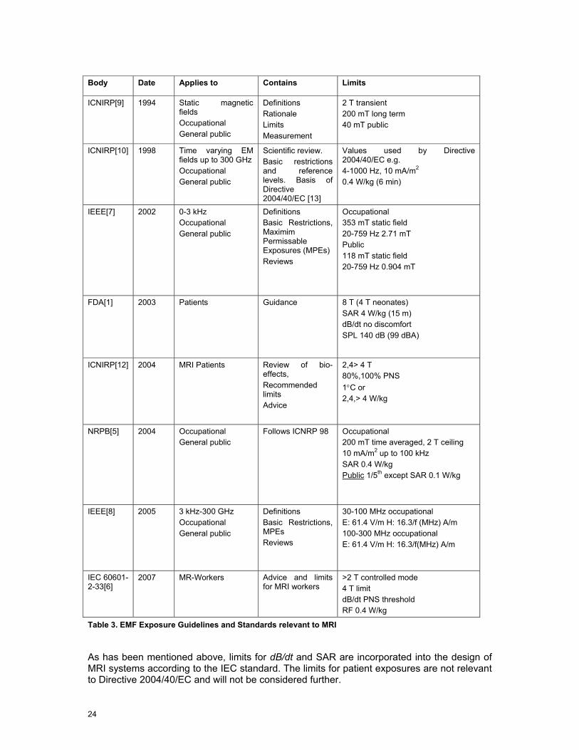
Body Date Applies to Contains Limits
ICNIRP[9] 1994 Static magnetic fields Occupational General public
Definitions Rationale Limits Measurement
2 T transient 200 mT long term 40 mT public
ICNIRP[10] 1998 Time varying EM fields up to 300 GHz Occupational General public
Scientific review. Basic restrictions and reference levels. Basis of Directive 2004/40/EC [13]
Values used by Directive 2004/40/EC e.g. 4-1000 Hz, 10 mA/m2 0.4 W/kg (6 min)
IEEE[7] 2002 0-3 kHz Occupational General public
Definitions Basic Restrictions, Maximim Permissable Exposures (MPEs) Reviews
Occupational 353 mT static field 20-759 Hz 2.71 mT Public 118 mT static field 20-759 Hz 0.904 mT
FDA[1] 2003 Patients Guidance 8 T (4 T neonates) SAR 4 W/kg (15 m) dB/dt no discomfort SPL 140 dB (99 dBA)
ICNIRP[12] 2004 MRI Patients Review of bio-effects, Recommended limits Advice
2,4> 4 T 80%,100% PNS 1°C or 2,4,> 4 W/kg
NRPB[5]
2004 Occupational General public
Follows ICNRP 98 Occupational 200 mT time averaged, 2 T ceiling 10 mA/m2 up to 100 kHz SAR 0.4 W/kg Public 1/5th except SAR 0.1 W/kg
IEEE[8] 2005 3 kHz-300 GHz Occupational General public
Definitions Basic Restrictions, MPEs Reviews
30-100 MHz occupational E: 61.4 V/m H: 16.3/f (MHz) A/m 100-300 MHz occupational E: 61.4 V/m H: 16.3/f(MHz) A/m
IEC 60601-2-33[6]
2007 MR-Workers Advice and limits for MRI workers
>2 T controlled mode 4 T limit dB/dt PNS threshold RF 0.4 W/kg
Table 3. EMF Exposure Guidelines and Standards relevant to MRI
As has been mentioned above, limits for dB/dt and SAR are incorporated into the design of MRI systems according to the IEC standard. The limits for patient exposures are not relevant to Directive 2004/40/EC and will not be considered further.
25
ICNIRP 2004 reviews PNS in humans which has been studied in MR gradient systems. A rheobase (minimum threshold) of 15 T/s for the y-gradient and 26 T/s is reported for the z-gradient. Y- and z-gradients refer to the switched spatially linear variations applied to the static field in the y- and z-directions, respectively. Chronaxies (time constants) for y- and z-gradients were reported as 0.365 and 0.378 ms respectively. A stimulus of 50% greater than threshold for sensation produces significant contracts, whilst 100% greater proves intolerable. It is helpful to describe the thresholds in terms of induced electric field E rather than current density as this removes uncertainties about tissue conductivity. The lowest rheobase is given as 2 V/m. Cardiac stimulation was achieved at 9 times the threshold for PNS in dogs. When scaled to human dimensions the threshold for cardiac stimulation is 405 T/s for a 2,503 µs current pulse width. The long chronaxie for cardiac stimulation of 3ms effectively reduces the risk to zero in MR current gradient systems where the stimulus durations are in the range 100-500 µs.
Transcranial magnetic stimulation (TMS) is another area where data on the neurological effects of dB/dt are well known. Brain stimulation requires E field of the order of 20 V/m. Induced fields of 1 to a few V/m can alter neuronal excitability if maintained for durations exceeding 10 ms. However the time required for this effect makes it unlikely to affect MRI where the induced field changes generally last less than 1 ms.
ICNIRP 2004 also addresses practical aspects of MR safety. These too are considered by other bodies (FDA, ACR, MHRA, IEC) and include the risks from ferromagnetic projectiles, pacemakers malfunction, RF heating from leads and cables, other implants and acoustic noise.
2.4.2 Other Occupational Limits In addition to ICNIRP occupational exposure to EMF has been considered by NRPB (NRPB 2004 [5]) and IEEE (IEEE 2002 [7], 2005 [8]). In general NRPB advice follows that of ICNIRP, resulting in substantially similar limits. IEEE occupational and general public limits are substantially different. See Table 3.
2.5 Acoustic Noise
Acoustic noise is generated essentially by Lorentz forces on the gradient coil mountings that arise when the currents in the gradient coils are switched within the static magnetic field. The spectral content of the noise generated is related to that of the input pulses to the gradient coil system. Noise level is measured in Pascal sound pressure level (SPL) or dB SPL with respect to 20 µPa or in dB(A) which is A weighted SPL. Typical noise levels on 1.5 T clinical MRI systems vary from about 80 dB(A) to 110 dB(A) depending on sequence type and on the degree of noise reduction technology implemented in the scanner design; levels can be higher on 3 T and ultrahigh field systems. A short term exposure 140 dB(SPL) can result in permanent damage to hearing (0dB (SPL)=220 µPa).
Standard IEC-60601-2-33 [6] requires that acoustic protection is provided to patients when the A-weighted r.m.s. sound pressure level is greater than 99 dB(A) (LAeq, 1 h and exposure is assumed to be sporadic and not daily). The standard does not define a value for MR workers for whom national standards and regulations must be applied. The UK’s MHRA recommends hearing protection to all patients at levels above 85 dB(A). Directive 2003/10/EC [14] of the European Parliament and of the Council of 6 February 2003 sets exposure limit values and exposure action values in respect of the daily noise exposure levels and peak sound pressure. In this case noise levels are averaged over an 8 hours working day. Exposure limit values are LEX,8h = 87 dB(A) and ppeak = 200 Pa SPL, respectively, at the ear (including the effects of any hearing protection). The provision of hearing protectors is required above the lower exposure action values: LEX,8h = 80 dB(A) and ppeak = 112 Pa SPL, respectively, whilst protection zones must be marked if levels are above the upper exposure action values: LEX,8h 85 dB(A) and ppeak = 140 Pa SPL, respectively.


27
3 Status Quo and Developments in Clinical MRI
3.1 Introduction
Traditionally Magnetic Resonance Imaging (MRI) has been associated with imaging the central nervous and musculoskeletal systems, but advances in technology that have allowed faster and more detailed scanning, have led to the routine use of MRI for diagnosis in most areas of the body and in most clinical specialties. MRI also offers the possibility of monitoring tissue function by measurement of molecular diffusion, blood flow and tissue perfusion as well as the possibility of using Magnetic Resonance Spectroscopy (MRS) to study biochemistry in-vivo. There is an increasing use of MRI for guidance, monitoring and controlling interventional and intra-operative procedures in view of its good spatial and temporal resolution, high intrinsic tissue contrast, and multi-planar imaging capabilities. Interventional MRI procedures are replacing X-ray based procedures resulting in avoidance of exposure of both patients and staff to ionizing radiation, although staff exposure to E-M fields may be increased in some cases to levels similar to those experienced by the patient or volunteer undergoing the procedure (Bassen et al 2005 [23]). A major research application of MRI is the study of normal brain anatomy and function, and this has been the main drive for the installation of dedicated research ultra-high field scanners over the last five years.
3.2 Electromagnetic Field Exposures in MRI
3.2.1 Static Field Exposure Most clinical MR scanners use superconducting magnets with cylindrical bores and produce static fields of magnetic flux density 1.5 T (Tesla), although there is now a significant number of 3 T scanners in clinical use. A smaller number of ultra-high field MR systems are in use in research institutions worldwide and these use static fields in the range 4.7 to 9.4 T. In general, traditional cylindrical bore systems restrict access to the patient, and present problems for imaging claustrophobic and obese patients. So-called open systems offer a more patient-friendly environment and provide much greater access to the patient, facilitating, for example, interventional procedures. Such systems use lower static fields, typically 0.2 – 1 T.
Although Directive 2004/40/EC [13] does not impose an exposure limit on the static magnetic field per se, workers moving through the spatially varying gradient of the static field close to a scanner will experience a time-varying field of low frequency (typically a few Hz) which will induce electric fields and a resulting current density within the body. Since the static field is maintained constantly, engineers who are required to carry out service work close or within the bore, nurses attending patients in special needs during examination, cleaners and radiographers who may be required work to and within the bore of the scanner will also be exposed to these electromagnetic fields. Crozier et al (2007) [26] have shown that movement induced electrical currents in tissues may exceed ICNIRP 1998 [10] limits.
3.2.2 EMF Exposure from the Imaging Gradients Three orthogonal gradients of the z-axis magnetic field are switched on and off to select the region of diagnostic interest and to spatially encode the MR signals. In general, the faster the imaging sequence, the greater the rate of change of the gradient fields required. These time-varying fields also lead to an induced electric field and consequent current density within the body. Typically, clinical MR systems generate gradient field strengths in the region of 25-50 mT/m and maximum slew rates (the peak field amplitude divided by the rise time) of 100 - 200 T/m/s within the imaging field of view. Gradient fields in ultra high field systems can be

28
as high as 100 mT/m with slew rates of 800 T/m/s. Gradient coil sets are designed to produce highly linear gradients within a region around the iso-centre of the scanner. However, these fields extend outside of the scanner housing and MRI workers standing close to the scanner whilst it is operating will be exposed to such fields. To date, little is known about the magnitude and directional geometry of these, although early studies demonstrate the possibility to exceed action values (McRobbie & Cross 2005 [41], Riches et al 2007 [47], Bradley et al 2007 [25], Crozier et al 2007 [26]). Typical frequencies are around 1 kHz but the spectral content of the gradient pulses can range from around 100 Hz up to 10 kHz. The trend towards shorter-bore magnets for greater patient comfort and acceptability is thought to result in an increase in the time-varying field dB/dt experienced by a worker positioned close to the bore entrance.
The performance goals of higher speed gradients are driven by MRI applications that require high speed imaging, including functional MRI, cardiac MRI, and diffusion measurements. High-speed imaging, in particular single-shot echo planar imaging, requires gradient slew rates clearly greater than 100-200 T/m/s and maximum levels over 20 mT/m. Functional MRI and cardiac MRI require both high slew rates and high gradient levels. This is particularly important in high-field MRI for which the increased signal can be traded for higher bandwidth image data acquisition. At least two factors may limit clinical application of high-field gradients. When the magnetic field varies by 60 T/s for longer than a few ms, nerve stimulation can be induced. This should be compared to the recommendation of 20 T/s for patient safety [6] and the ICNIRP guidelines [10] for time derivate of the magnetic field dB/dt of 0.22 T/s for occupational exposure in the low frequency range. A second problem is acoustic noise, which is reaching unbearable levels with the newest gradients when these are operating at their maximum switching rates, resulting in sound pressure level in excess of 100 dB(A) and the UK’s MHRA recommends hearing protection to all patients at levels above 85 dB(A).
3.2.3 Radiofrequency Exposures The RF field is applied at the Larmor frequency ωo = γ Bo where γ is the gyromagnetic ratio. For hydrogen as imaged in MRI, γ = 42.58 MHz /T; thus the RF frequency at 1, 1.5, 3, and 7 T is 42.58, 63.87, 127.74 and 298.06 MHz, respectively. The main transmitter coil is usually a body coil, integrated into the scanner that produces a circularly polarised B1 field. In conventional cylindrical bore systems at 1.5 or 3 T, this is usually a birdcage coil designed to achieve a region around the iso-centre of the coil in which the B1-field is spatially uniform. In open MR scanners in which the static field is vertical, a circularly polarised B1-field is often produced by a pair of planar coils placed above and below the patient. In some examinations such as those of the head, other transmitter coils are often used. For MRI only the magnetic field component (H or B) is required. The E field is generally small except in the vicinity of the coil windings.
In general occupational exposure to the B1 field will be low since the field falls off rapidly outside the transmit coil. However, an exception will be staff carrying out interventional procedures, particularly in open scanners, where hands and arms, and possibly the head may be exposed to levels similar to those experienced by the patient or volunteer undergoing the procedure (Bassen et al 2005 [23]).
3.3 Future Trends in MRI Applications
There is a clear trend to higher field strength scanners (e.g. 3 T) for clinical use and in research, the use of ultra-high systems for structural imaging (Elster 1999 [29], Nakada 2007 [45], Regatte & Schweitzer 2007 [46]). The detailed monitoring the effectiveness of anti-angiogenetic and genetic based drugs, and molecular applications such as quantitative imaging of gene expression, marking stem cells and tracking their evolution or targeting

29
malignant cells with targeted contrast agents drives the demand for higher field strengths (Rogers et al 2006 [48], Grimm et al 2007 [31]).
There is also likely to be increased interest in lower field open scanners with superconducting magnets at 1 T, or very short-bore 1.5 T cylindrical systems for intra-operative (e.g. MR guidance for surgery) and interventional (e.g. MR guidance/monitoring) procedures (Grönemeyer 1999 [32], Gedroyc 2000 [30], Hailey 2006 [33]). Open-bore magnets also offer advantages for scanning claustrophobic patients (Bangard et al 2007 [22]).
Interventional cardiovascular magnetic resonance imaging (iCMR) refers to catheter-based therapeutic procedures using MRI rather than conventional radiographic guidance permitting surgical-quality “exposure” in minimally invasive procedures (Lederman 2005 [38], Saborowski & Saeed 2007 [83]). iCMR is possible due to technical advances such as highly uniform magnetic fields, rapidly changeable magnetic field gradients, multi-channel receivers and advanced computing systems (Duerk et al 2000 [27], Duerk 2002 [28]). Some specific technical problems still make MR-guided interventions challenging: in mid-field (B0 > 1 T) MRI scanners, access to the patient is limited owing to the closed bore construction of the MR magnet. Furthermore, gradient noise makes communication between interventionalist, nurse and scanner operator difficult or even impossible (Bock et al 2005 [24]). Nevertheless high field systems have also been used for interventional procedures (Hall et al 1999 [35]).
It is also likely that more systems will be installed outside of the traditional hospital radiology settings, e.g. in cardiology and orthopaedics hospital departments, and also in primary care units.
Figure 1. Publications relating to iMR by year .
Figure 2. Interventional MR publications by clinical area
Figure 1 shows the number of scientific publications per annum relating to interventional MR since its inception around 1990, clearly demonstrating an increasing interest in this new application. Figure 2 shows the breakdown of these publications by area. In addition to iCMR, these include head and neck (Lufkin et al 1990 [40], Hall et al 1999 [34]), breast (Hall-Craggs 2000 [35], Floery & Helbich 2006 [85]), liver (Clasen et al 2007 [86]), female pelvis
0
10
20
30
40
50
60
70
1990 1991 1992 1993 1994 1995 1996 1997 1998 1999 2000 2001 2002 2003 2004 2005 2006 2007
IMR papersIMR reviews
iMR publications 1990-2007
0 20 40 60 80 100
Female Pelvis
GI tract
Paediatric
Renal
Breast
Liver
Economics
Prostate
MSK
Safety
Non specific
Cardio-vascular
Neuro
Technical

30
(Brown et al 2006 [92]). Interventional MR utilises a range of therapies including various ablative techniques: microwave (Kurumi et al 2007 [37]), cryogenic (Mogami et al 2007 [43]), radiofrequency (Clasen et al 2007 [86]), focused ultrasound (de Senneville et al 2007 [49]), in addition to providing image guidance for biopsies and aspiration (Lewin JS et al 2000[39]) and laparoscopic and robotic surgery (Hashizume 2007 [36]). Much effort has gone into the technological developments needed to perform interventional procedures safely in the MR environment. Technical articles largely account for the peak at around year 2000.
3.4 Other Areas of MR Potentially Affected by Directive 2004/40/EC
Other areas where staff are likely to experience EMF exposures include the scanning of vulnerable patients (mental health, children, claustrophobic), monitoring of patients during general anaesthesia and sedation, and manual administration of contrast agents. Recently two surveys have taken place, one by the European Society of Radiology and the other by the British Association Radiographers. Table 4 contains the ESR findings, showing that scanning of children and general anaesthesia account for 6% of MRI scan in the EU, or 480,000 scans per annum.
The British Association of MR Radiographers survey (Moore & Scurr 2007 [44]) indicates that approximately 3% of all MRI examinations in the UK require a member of staff present in the magnet room during scanning. The most common reasons for remaining in the MR examination room were monitoring of GA patient, accompanying a claustrophobic patient, or manual contrast administration. Other potential exposures included prison officers accompanying a patient and interpreters. MR contrast agents can be administered remotely by injection pump, however for some patients (very young or very sick), a manual administration is preferable.
Type Examination Total % of total Procedures studied in the current contract
Total number of MRI exams 8,000,000 100
Procedures with contrast 2,000,000 25 Strasbourg C3
Nottingham C1
Procedures in children 400,000 5 Cologne C3
Strasbourg C1
Strasbourg C2
Leuven C3
Procedures under anaesthesia 80,000 1 Cologne C3
Strasbourg C1
Leuven C3
Interventional MRI
(thermo-ablation, RF, laser, cryo)
2000 0.025 Cologne C2
MRI-guided biopsies 5000 0.0625 Cologne C1
Intra-operative MRI 500 0.00625 Table 4. MR examinations in the EU (from G Krestin, ESR)
4 Observation of Clinical Procedures - Method
4.1 Participating Centres
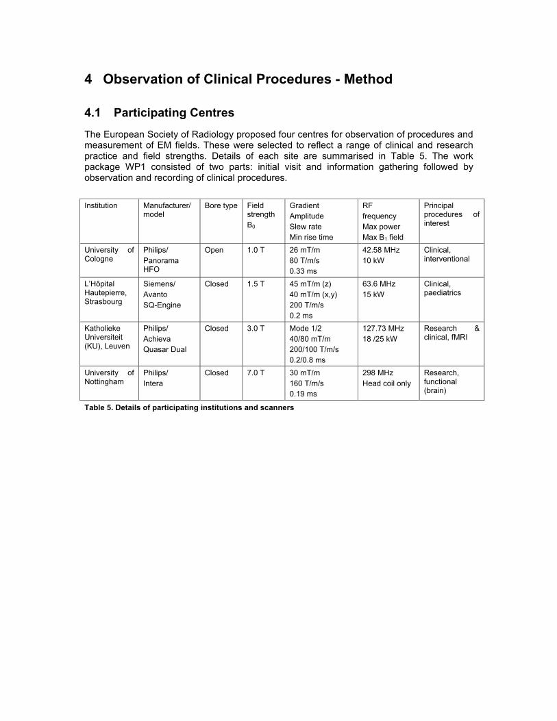
The European Society of Radiology proposed four centres for observation of procedures and measurement of EM fields. These were selected to reflect a range of clinical and research practice and field strengths. Details of each site are summarised in Table 5. The work package WP1 consisted of two parts: initial visit and information gathering followed by observation and recording of clinical procedures.
Institution Manufacturer/
model Bore type Field
strength B0
Gradient Amplitude Slew rate Min rise time
RF frequency Max power Max B1 field
Principal procedures of interest
University of Cologne
Philips/ Panorama HFO
Open 1.0 T 26 mT/m 80 T/m/s 0.33 ms
42.58 MHz 10 kW
Clinical, interventional
L’Hôpital Hautepierre, Strasbourg
Siemens/ Avanto SQ-Engine
Closed 1.5 T 45 mT/m (z) 40 mT/m (x,y)
200 T/m/s 0.2 ms
63.6 MHz 15 kW
Clinical, paediatrics
Katholieke Universiteit (KU), Leuven
Philips/ Achieva Quasar Dual
Closed 3.0 T Mode 1/2 40/80 mT/m 200/100 T/m/s 0.2/0.8 ms
127.73 MHz 18 /25 kW
Research & clinical, fMRI
University of Nottingham
Philips/ Intera
Closed 7.0 T 30 mT/m 160 T/m/s 0.19 ms
298 MHz Head coil only
Research, functional (brain)
Table 5. Details of participating institutions and scanners
32
4.2 Sites and MRI Machines
Four MRI machines have been selected for consideration within this project, each has a different static magnetic field, three are traditional cylindrical bore machines and one is an open MRI.
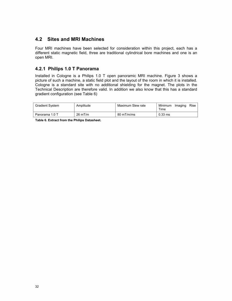
4.2.1 Philips 1.0 T Panorama Installed in Cologne is a Philips 1.0 T open panoramic MRI machine. Figure 3 shows a picture of such a machine, a static field plot and the layout of the room in which it is installed. Cologne is a standard site with no additional shielding for the magnet. The plots in the Technical Description are therefore valid. In addition we also know that this has a standard gradient configuration (see Table 6)
Gradient System Amplitude Maximum Slew rate Minimum Imaging Rise
Time Panorama 1.0 T 26 mT/m 80 mT/m/ms 0.33 ms
Table 6. Extract from the Philips Datasheet.

33
Figure 3 Philips 1.0 T Panorama. Field plots and picture from the manufacturer’s data sheet and the actual room plan of the site in Cologne.

34
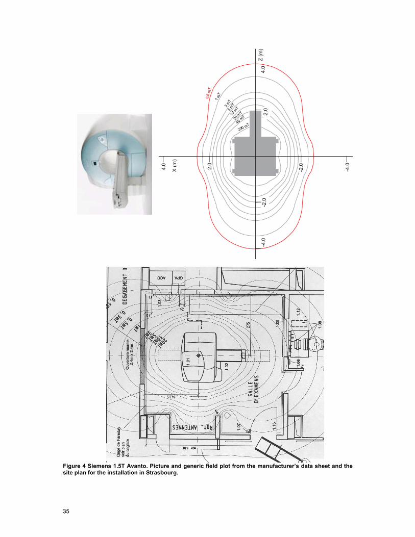
4.2.2 Siemens 1.5 T Avanto Installed in Strasbourg is a Siemens 1.5 T Avanto system, Figure 4 shows an illustration of the machine, the floor plan of the MRI suite and the static fields in the absence of additional shielding. The gradient performance depends on the installed option; upper limits are shown in Table 7.
Gradient system (Tim 76x18) SQ-engine Performance per axis Max. amplitude 45 mT/m Min. rise time 200 µs from 0 to 40 mT/m Max. slew rate 200 T/m/s Vector gradient performance (vector summation of all 3 gradient axes) Max. eff. amplitude 72 mT/m Max. eff. slew rate 346 T/m/s
Table 7. Extract from the Siemens data sheet.
35
Figure 4 Siemens 1.5T Avanto. Picture and generic field plot from the manufacturer’s data sheet and the site plan for the installation in Strasbourg.

36
4.2.3 Philips 3.0 T Achieva For the Philips 3.0 T Achieva in Leuven the magnet is shielded on one side to reduce the stray field in the hallways adjacent to the system to a level < 0.5 mT. This passive shielding was produced by a local organisation and not the manufacturer so no field plots of the resulting stray field are available. Figure 5 shows an illustration of the machine, floor plan of the mRI suite and the static fields prior to shielding
The machine in Leuven is equipped with the Quasar Dual gradient system which has the possibility of higher slew rates and amplitudes (see Table 8).
Figure 5. Philips 3.0 T Achieva. Picture and field plot from the manufacturer’s datasheet and the Leuven site plan.

37
Gradient System Amplitude Maximum
Slew Rate Minimum Imaging Rise Time
Quasar 40 mT/m 120 mT/m/ms 0.33 ms Quasar Dual ---Mode 1 40 mT/m 200 mT/m/ms 0.20 ms ---Mode 2 80 mT/m 100 mT/m/ms 0.80 ms
Table 8. Extract from the specification in the Philips datasheet.

38
4.2.4 Philips 7.0 T Intera Installed in Nottingham and Zurich are Philips 7.0 T Intera machines, these machines have substantial magnetic shielding and this is reflected on the static field plot (see Figure 6).
Figure 6 Philips 7.0 T Intera. Picture courtesy of UniversitätsSpital Zürich (USZ) and field plot from Nottingham.

39
4.3 Initial Visits
A questionnaire was devised to assist with the information gathering. The questionnaire covered the technical specifications of the scanner, the range of clinical procedures, emergency procedures, anaesthesia/sedation policy, and contrast agent administration and local safety protocols. This was sent to the participating centres prior to the initial visit. The completed questionnaires are contained in Appendix B.1.
In the initial stage, a minimum of two consortium members visited each centre. For three out of the four visits, they were accompanied by M. G Herbillon, representative of the European Commission’s Directorate General for Employment, Social Affairs and Equal Opportunities. The initial visits were carried out between August 2 and September 3. At the initial visit, the questionnaires were completed and a discussion took place concerning the most important clinical procedures to investigate with respect to directive 2004/40/EC. Centres were advised of the scope and purpose of the project and of the need to consider the ethics of filming clinical procedures. Additionally the MR room was surveyed for suitability for access for the video equipment. Where available, MR scanning protocols were collected, as were photographs of the rooms and room plans. At the initial visit, dates for the measurement visits were determined. The questionnaires were returned to the centres for further reference. Visits to the manufacturers (Siemens and Philips) also took place on 21, 22 August 2007.
4.4 Video Visits
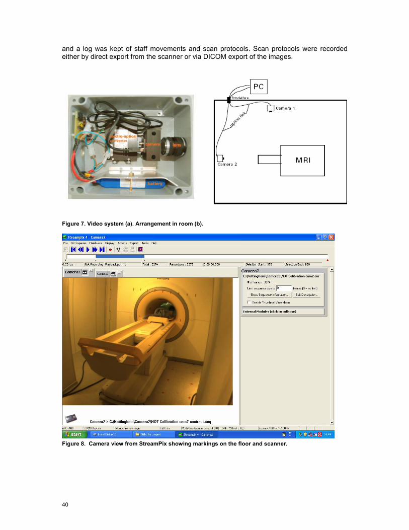
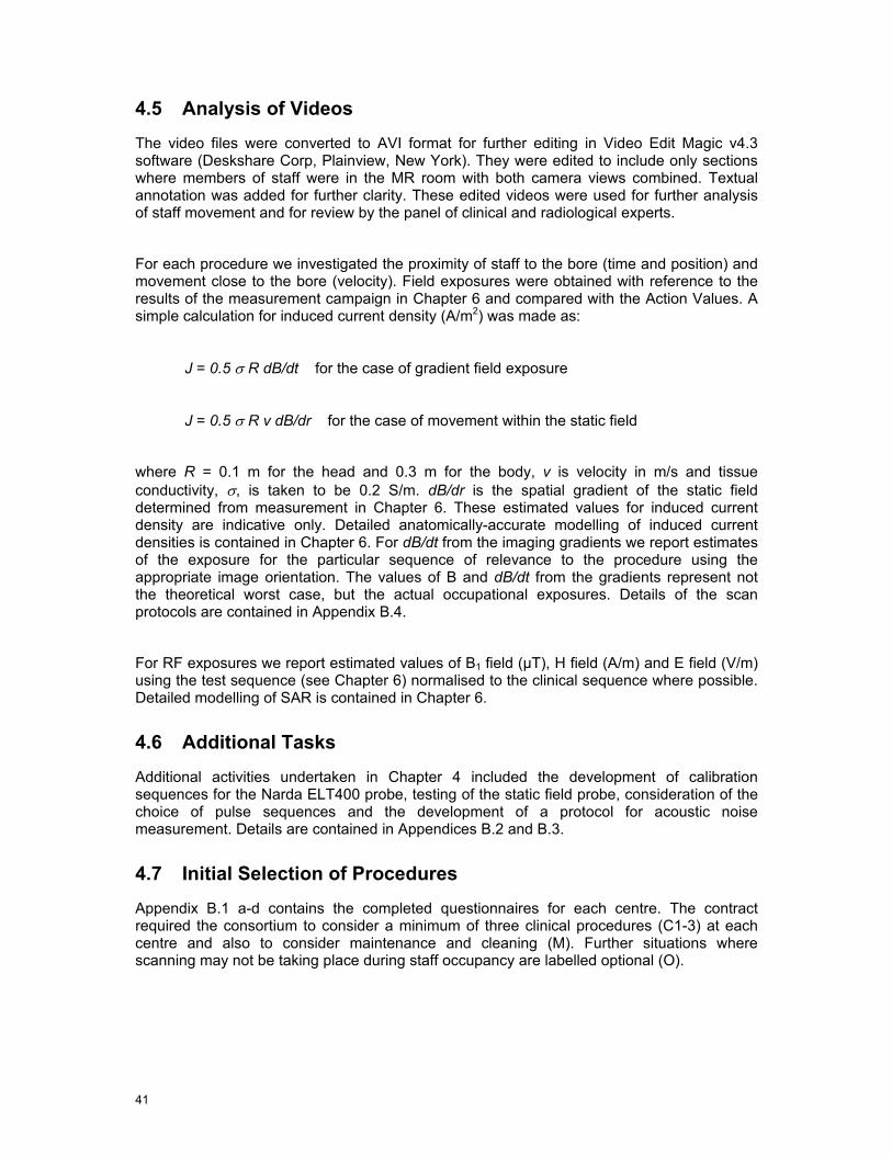
4.4.1 Video Recording System MR compatible video equipment was produced by IT’IS. Two MR compatible video cameras were sourced (AVT GUPPY F-033C) and installed in RF shielded, non-ferromagnetic cases. The cameras were interfaced to the video acquisition computer using IEEE 1394b, with 20 m optical cables run from either the MR equipment room or control room through existing waveguides. MR compatible rechargeable lithium polymer (LiPo) batteries were used, with lifetime of 12 hours. The cameras provided a maximum resolution of 640x494 pixels at frame rates up to 60 Hz (25 typical) in colour with 8-bit depth. The lens focal length was 4.2 mm giving a horizontal field of view of greater than 3 m at 3 m distance. The data acquisition storage was greater than 1 TByte. The video recording software was Streampix (Norpix Inc, Montreal, Quebec). This enabled simultaneous recording of both video streams. Figure 7a and Figure 7b show a schematic diagram and photograph of the camera system.
The system was tested at Zurich in the 7.0 T Philips scanner at USZ. Additionally in Leuven (Philips 3.0T) the system was tested in situ for its effect on scanner signal-to-noise ratio and possible induction of image artefacts prior to its being used for recording actual patient procedures.
4.4.2 Method on Site For each centre, the ideal measurement arrangement would be to have one camera positioned on the scanner axis looking along the bore, with the second positioned orthogonally looking across the long axis of patient couch (Figure 7b). However, due to the room layouts this was not possible for all systems. Actual camera positions are shown in the relevant sections below. In Nottingham, three separate combinations of camera positions were used to capture different staff activities. For each centre, markings were positioned on the scanner and on the floor. For the floor, a grid of 50 cm resolution was created using plastic coloured tape. Linear markings at 20 cm spacing were placed along the patient couch and across the front face of the magnet above the bore entrance (Figure 8). A similarly marked wooden pole was used to calibrate the video recording of the floor grid. Synchronisation of the video stream was achieved using a standard photographic flash unit fired at the beginning of the procedure. During procedures, the cameras were left running
40
and a log was kept of staff movements and scan protocols. Scan protocols were recorded either by direct export from the scanner or via DICOM export of the images.
Figure 7. Video system (a). Arrangement in room (b).
Figure 8. Camera view from StreamPix showing markings on the floor and scanner.
41
4.5 Analysis of Videos
The video files were converted to AVI format for further editing in Video Edit Magic v4.3 software (Deskshare Corp, Plainview, New York). They were edited to include only sections where members of staff were in the MR room with both camera views combined. Textual annotation was added for further clarity. These edited videos were used for further analysis of staff movement and for review by the panel of clinical and radiological experts.
For each procedure we investigated the proximity of staff to the bore (time and position) and movement close to the bore (velocity). Field exposures were obtained with reference to the results of the measurement campaign in Chapter 6 and compared with the Action Values. A simple calculation for induced current density (A/m2) was made as:
J = 0.5 σ R dB/dt for the case of gradient field exposure
J = 0.5 σ R v dB/dr for the case of movement within the static field
where R = 0.1 m for the head and 0.3 m for the body, v is velocity in m/s and tissue conductivity, σ, is taken to be 0.2 S/m. dB/dr is the spatial gradient of the static field determined from measurement in Chapter 6. These estimated values for induced current density are indicative only. Detailed anatomically-accurate modelling of induced current densities is contained in Chapter 6. For dB/dt from the imaging gradients we report estimates of the exposure for the particular sequence of relevance to the procedure using the appropriate image orientation. The values of B and dB/dt from the gradients represent not the theoretical worst case, but the actual occupational exposures. Details of the scan protocols are contained in Appendix B.4.
For RF exposures we report estimated values of B1 field (µT), H field (A/m) and E field (V/m) using the test sequence (see Chapter 6) normalised to the clinical sequence where possible. Detailed modelling of SAR is contained in Chapter 6.
4.6 Additional Tasks
Additional activities undertaken in Chapter 4 included the development of calibration sequences for the Narda ELT400 probe, testing of the static field probe, consideration of the choice of pulse sequences and the development of a protocol for acoustic noise measurement. Details are contained in Appendices B.2 and B.3.
4.7 Initial Selection of Procedures
Appendix B.1 a-d contains the completed questionnaires for each centre. The contract required the consortium to consider a minimum of three clinical procedures (C1-3) at each centre and also to consider maintenance and cleaning (M). Further situations where scanning may not be taking place during staff occupancy are labelled optional (O).

42
1 T Open Cologne Interventional
1.5 T Strasbourg Diagnostic Clinical with Paediatrics
3 T Leuven Diagnostic Clinical
7 T Nottingham Research
C1 Performing breast biopsy Monitoring of GA procedure
Clinical fMRI (tactile stimulus)
Manual contrast injection - Angiography
C2 Guide wire placement (breast)
Parent or member of staff with child in scanner
Cardiac stress test EEG experiment (positioning only)
C3 Manual contrast administration to child
Intensive care patient on respirator
Paediatric GA (1.5 T)
Evacuating patient in emergency
O Emergency evacuation Emergency evacuation Manual contrast injection
M Cleaning/maintenance within bore
Cleaning/maintenance within bore
Cleaning/maintenance within bore
Maintenance, e.g. coil adjustment, within bore
Dates Sep 26 – 27 Oct 2 - 3 Sep 24 - 26 Oct 12
Table 9. Initial choice of procedures.
Table 9 shows that only certain procedures definitely involve staff being present during scanning with potential exposure to low frequency time-varying magnetic fields dB/dt from the gradients and radio-frequency fields. These are from Cologne C2; Strasbourg C1, C2, C3; Leuven C1, C2, C3; Nottingham C1.
From our initial visits and the analysis of the questionnaire responses we were able to determine the worst case situations for each scanner in terms of the choice of pulse sequence and likely staff exposure. In particular, sequences involving rapid scanning with high slew rate gradients were identified, especially echo planar imaging (EPI) and steady state free precession sequences (SSFP). These latter are denoted Balanced-FFE/TFE on Philips scanners and TrueFISP on Siemens scanners.
4.8 Sequences
Pulse sequence diagrams show the relative timing of the imaging gradients and RF pulses. These are normally labelled according to their role in image formation i.e. slice select (SS), phase encode (PE) and frequency encode (FE), rather than their physical orientation: x, y, z.
Figure 9 shows the relationship between image planes and physical gradient coils.
Each of Gx Gy and Gz is generated by a separate physical gradient coil contained within the bore of the magnet. Details of coils are contained in Chapter 6. In any given clinical situation each imaging gradient (GSS etc.) may contain components of one or more physical gradients x, y, z. For a simple transverse or axial slice, GSS only uses the z gradient coil, and the other

43
two image formation gradients usually conform to x and y. In general the gradient amplitude will scale linearly with image field of view and slice thickness, so in order to achieve a higher spatial resolution in the image, larger gradients are required. The RF pulse shape may also change with changing slice thickness, and the exposure in terms of SAR is affected by the number of slices, the ‘flip angle’, the number of echo signals acquired and the sequence repetition time, TR.
Table 10 summarises the initial selection of pulse sequences using data from the initial site visits. The criteria for their selection was based upon their use during procedures that require staff to be close to the magnet during scanning and the relative amplitude of gradients and RF in each. Details can be found in any standard MR textbook (e.g. McRobbie et al 2007).
Physical Orientation Orientation Slice Phase Frequency Transverse Z X or Y Y or X Sagittal X Y or Z Z or Y Coronal Y X or Z Z or X
Figure 9. Image planes and gradient axes. From MRI from Picture to Proton (McRobbie et al 2007).
Exposure Philips scanners Siemens scanners
bFFE/bTFE TrueFISP FE-EPI GE-EPI DW-EPI (secondary) DW-EPI (secondary)
Gradients
Any other identified from initial visits Multi-slice T2-TSE with DRIVE Multi-sliceT2-TSE with restore B-FFE (secondary) TrueFISP (secondary)
RF
Any other identified from initial visits
Table 10. Initial choice of pulse sequences for investigation. See abbreviations list for explanation.

44
4.8.1 Balanced-FFE/TrueFISP
Figure 10. Gradient and RF waveforms for bFFE/TrueFISP. From MRI from Picture to Proton (McRobbie et al 2007).
The balanced-FFE/TFE or TrueFISP sequence is typically used for real-time scanning where a high image quality is required such as in guiding interventional procedures, e.g. biopsies and cardiac scanning. The slice select gradients (GSS), phase encode gradients (GPE), frequency encode gradients (GFE) and RF pulse waveforms are illustrated in Figure 10. The portion shown represents one line of the data acquisition, typically being repeated 128 or 256 times to form a 2D image.
The pulses shown are repeated in an identical manner with the exception of the phase encode gradient, GPE, which incrementally steps through a range of values. Both GSS and GFE are likely to produce the maximum exposures in terms of B and dB/dt. At times when these overlap the exposure will consist of the vector sum of the individual components.
4.8.2 Echo-Planar Imaging Echo planar imaging (EPI) is a very rapid MR sequence used primarily in situations where physiological and gross motion needs to be frozen such as in diffusion-weighted imaging (DWI), diffusion tensor imaging (DTI), functional MRI brain activation studies (fMRI) or perfusion imaging.
Figure 11. EPI sequence gradient waveforms. From MRI from Picture to Proton (McRobbie et al 2007).

45
The sequence acquires one image in a single acquisition or shot, and is characterised by the rapidly switched bipolar frequency encode gradient GFE (see Figure 11). This sequence sometimes triggers the scanner’s Peripheral Nerve Stimulation (PNS) monitor, particularly if images are acquired in the coronal plane. Consequently this gradient is likely to dominate the exposure level. The gradient strengths are likely to scale inversely with image field-of-view (FOV).
4.8.3 Diffusion-Weighted / Diffusion Tensor Imaging Diffusion weighted or tensor imaging is a spin echo EPI sequence, with additional strong gradients used to generate the diffusion sensitivity. These diffusion gradients, shown in the lighter shade in Figure 12, are generally applied at maximum gradient amplitude with a high slew rate. Gradient pulses may be applied on different gradient coils simultaneously, giving a greater resultant field. These are likely to be played out at maximum amplitude and slew rate and do not scale with the FOV.
Figure 12. Diffusion-weighted EPI sequence. From MRI from Picture to Proton (McRobbie et al 2007).
4.8.4 T2-Weighted Turbo Spin Echo The T2-weighted turbo spin echo sequence is a standard clinical sequence used in most imaging protocols, including paediatric brain (under GA). It is characterised by a series of RF generated ‘spin echoes’ (see Figure 13). The addition of extra 180° RF pulses greatly adds to the RF exposure. This sequence will occasionally exceed IEC Level I for SAR. It is the worst case in terms of potential RF exposure. In general, SAR will increase with the number of echoes, slices and size of flip angle (power of RF pulses). The sequence may also be performed in a single-shot format, sometimes called single shot turbo spin echo (SS-TSE) or half Fourier acquisition single shot turbo spin echo (HASTE).
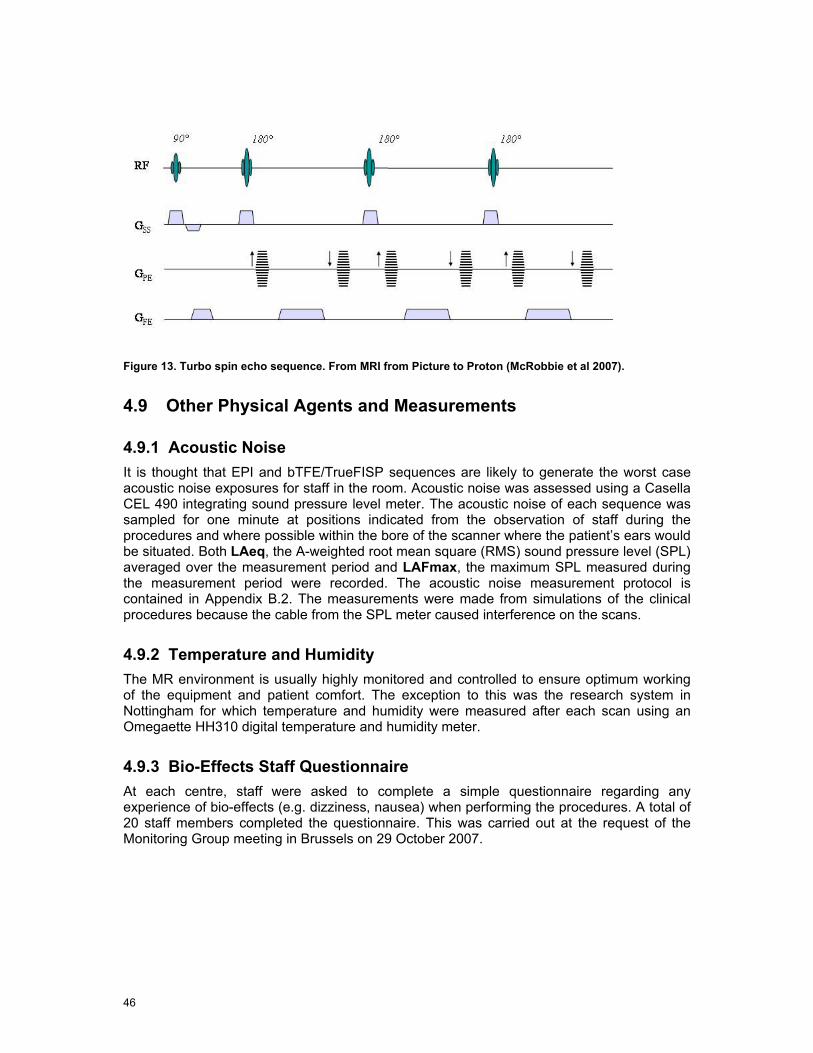
46
Figure 13. Turbo spin echo sequence. From MRI from Picture to Proton (McRobbie et al 2007).
4.9 Other Physical Agents and Measurements
4.9.1 Acoustic Noise It is thought that EPI and bTFE/TrueFISP sequences are likely to generate the worst case acoustic noise exposures for staff in the room. Acoustic noise was assessed using a Casella CEL 490 integrating sound pressure level meter. The acoustic noise of each sequence was sampled for one minute at positions indicated from the observation of staff during the procedures and where possible within the bore of the scanner where the patient’s ears would be situated. Both LAeq, the A-weighted root mean square (RMS) sound pressure level (SPL) averaged over the measurement period and LAFmax, the maximum SPL measured during the measurement period were recorded. The acoustic noise measurement protocol is contained in Appendix B.2. The measurements were made from simulations of the clinical procedures because the cable from the SPL meter caused interference on the scans.
4.9.2 Temperature and Humidity The MR environment is usually highly monitored and controlled to ensure optimum working of the equipment and patient comfort. The exception to this was the research system in Nottingham for which temperature and humidity were measured after each scan using an Omegaette HH310 digital temperature and humidity meter.
4.9.3 Bio-Effects Staff Questionnaire At each centre, staff were asked to complete a simple questionnaire regarding any experience of bio-effects (e.g. dizziness, nausea) when performing the procedures. A total of 20 staff members completed the questionnaire. This was carried out at the request of the Monitoring Group meeting in Brussels on 29 October 2007.

5 Observation of Clinical Procedures - Results and Analysis
The video measurements were made between 26 September and 12 October 2007 as detailed in Table 11. The final choice of procedures was determined by the actual cases available on the days of the visits. Additionally some procedures were videoed on the 1.5 T Philips system in Leuven because these procedures are currently carried out only at 1.5 T but may migrate to 3T in the future.
1.0 T Open Cologne Interventional
1.5 T Strasbourg Diagnostic Clinical with Paediatrics
3.0 T Leuven Diagnostic Clinical
7.0 T Nottingham Research
C1 Performing breast biopsy Monitoring of GA procedure
Clinical fMRI (tactile stimulus)
Manual contrast injection
C2 Clip placement (breast) Parent or member of staff with child in scanner
Cardiac stress test (1.5 T)
EEG experiment (positioning only)
C3 GA of child Manual contrast administration
Paediatric GA (1.5 T)
Evacuating patient in emergency
O Emergency evacuation Emergency evacuation Emergency evacuation
M Cleaning/maintenance within bore
Cleaning/maintenance within bore
Adjustment same as C2
Dates Sep 26–27 2007 Oct 2–3 2007 Sep 24–26 2007 12 Oct 2007
Table 11. Actual Video Measurements.
The coordinate system used throughout the document uses the isocentre as the reference point for all measurements. The isocentre is the point in the centre of the bore of the MRI machine about which images are acquired, denoted as (0, 0, 0). The axis directions are shown in Figure 14, this is irrespective of machine type (for the open the z – direction is along the table).
Y
X
Z
Figure 14. Coordinate system directions.

48
5.1 Cologne 1.0 T
System 1.0 T Open
Purpose Interventional
Procedures C1 Performing breast biopsy
C2 Clip placement (breast)
C3 General anaesthesia of child x3 (No one in room) but parent in room x1
O Simulation of emergency evacuation
M Cleaning not observed at visit. This is carried out by a specialist team.
Video camera placement is shown in Figure 15.
Figure 15. Camera placement and acoustic noise measurement positions, Cologne.
5.2 Procedures
C1 Breast Biopsy
This is important for patients with clinical symptoms and a family history of breast cancer where ultrasound and mammography have proved negative. The biopsy is not performed during scanning.
1
2
3
4
5
6
49
The scan protocol was as follows
Localiser
Dynamic contrast
Balanced turbo field echo (sBTFE)
Scan to confirm position
Protocol names in brackets are those set on the scanner by the host institution. Details of the scan parameters can be found inAppendix B.4.
Two members of staff, the radiologist and the radiographer entered the room, but not during scanning. Table 9 summarises their actions. The radiologist performs the biopsy whilst scanning is stopped. The couch is brought out and he is seated at position x = -40 cm; y= 0 cm; z = -136 cm with respect to the isocentre (0,0,0) for 4 min 8 sec as shown in Figure 16 (two simultaneous camera views).

50
Time mm:ss
Activity
00:00 Start of video 02:35 Patient enters with radiographer Survey & Dynamic contrast 18:50 Radiologist enters to adjust biopsy location phantom. No scanning. Position scan 21:15 Radiologist and technician enter to prepare biopsy area. No scanning 27:00 Left room. Position check scan. 28:00 Radiologist enters room and performs biopsy. No scanning Confirmation scan 32:00 Radiologist and technician enter to bandage and remove patient. No scanning 42:00 End of procedure. Patient leaves 48:38 End of recording
Table 12. Breast biopsy staff activities.
Figure 16. Breast biopsy. No scanning is performed during the actual biopsy.
C2 Clip Placement (breast)
Only one procedure in Cologne involved a member of staff (the radiologist) being within the MR room during scanning. This was a clip placement in the breast to indicate the position of a tumour, treated by chemo-therapy and prior to surgery. The presence of the clip enables the correct identification of the tumour site for surgery. The procedure is not possible using alternative methods: ultrasound or mammography. The scan protocol is similar to the breast biopsy protocol.
During the procedure the radiologist positions the clip using real-time imaging (balanced-TFE). This involves being positioned within the magnet adjacent to the patient for about 30 seconds. Table 13 summarises staff movements for the radiologist and the radiographer.
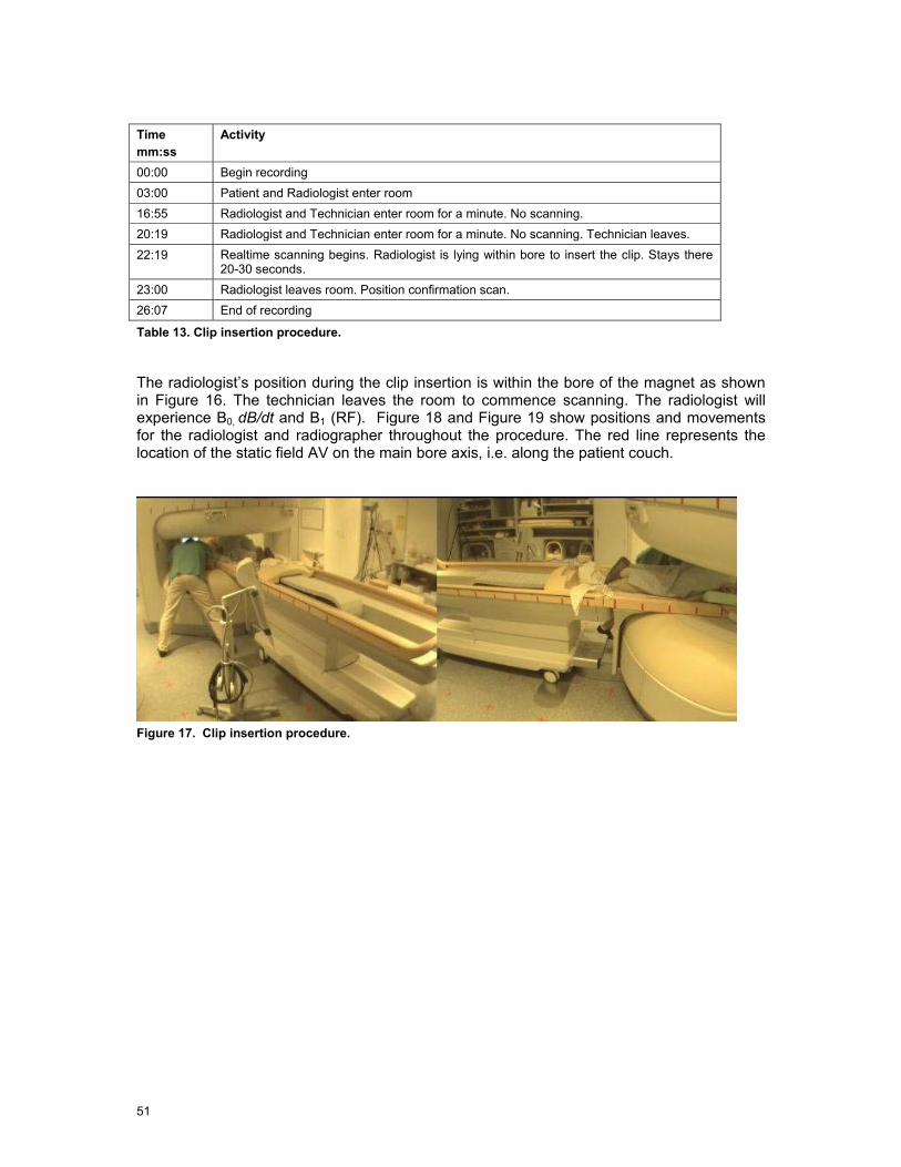
51
Time mm:ss
Activity
00:00 Begin recording 03:00 Patient and Radiologist enter room 16:55 Radiologist and Technician enter room for a minute. No scanning. 20:19 Radiologist and Technician enter room for a minute. No scanning. Technician leaves. 22:19 Realtime scanning begins. Radiologist is lying within bore to insert the clip. Stays there
20-30 seconds. 23:00 Radiologist leaves room. Position confirmation scan. 26:07 End of recording
Table 13. Clip insertion procedure.
The radiologist’s position during the clip insertion is within the bore of the magnet as shown in Figure 16. The technician leaves the room to commence scanning. The radiologist will experience B0, dB/dt and B1 (RF). Figure 18 and Figure 19 show positions and movements for the radiologist and radiographer throughout the procedure. The red line represents the location of the static field AV on the main bore axis, i.e. along the patient couch.
Figure 17. Clip insertion procedure.
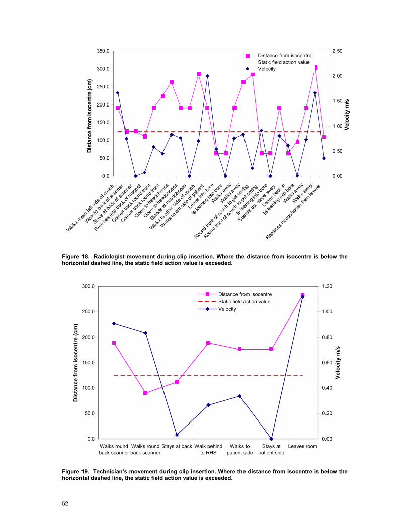
52
0.0
50.0
100.0
150.0
200.0
250.0
300.0
350.0
Walks do
wn left s
ide of c
ouch
Walk to ba
ck of
scan
ner
Stays a
t back
of sca
nner
Reache
s into
back
of mag
net
Comes
back
roun
d fron
t
Comes
back
roun
d fron
t
Goes t
o hea
dpho
nes
Goes t
o hea
dpho
nes
Stands a
t hea
dphon
es
Walks to
other s
ide of c
ouch
Walks t
o left s
ide of p
atien
t
Lean
s into
bore
Is lea
ning i
nto bo
re
Walks
away
Walks
away
Round fro
nt of
couch
to get
smthg
Round f
ront o
f couc
h to g
et sm
thg
Is lea
ning into
bore
Stands u
p, ste
ps aw
ay,
Leans b
ack in
Is lea
ning i
nto bo
re
Walk
s away
Walks aw
ay
Replac
es he
adpho
nes th
en lea
ves
Dist
ance
from
isoc
entr
e (c
m)
0.00
0.50
1.00
1.50
2.00
2.50
Velo
city
m/s
Distance from isocentreStatic field action valueVelocity
Figure 18. Radiologist movement during clip insertion. Where the distance from isocentre is below the horizontal dashed line, the static field action value is exceeded.
0.0
50.0
100.0
150.0
200.0
250.0
300.0
Walks roundback scanner
Walks roundback scanner
Stays at back Walk behindto RHS
Walks topatient side
Stays atpatient side
Leaves room
Dis
tanc
e fr
om is
ocen
tre
(cm
)
0.00
0.20
0.40
0.60
0.80
1.00
1.20
Velo
city
m/s
Distance from isocentreStatic field action valueVelocity
Figure 19. Technician’s movement during clip insertion. Where the distance from isocentre is below the horizontal dashed line, the static field action value is exceeded.
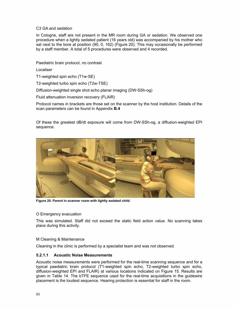
53
C3 GA and sedation
In Cologne, staff are not present in the MR room during GA or sedation. We observed one procedure when a lightly sedated patient (16 years old) was accompanied by his mother who sat next to the bore at position (90, 0, 162) (Figure 20). This may occasionally be performed by a staff member. A total of 5 procedures were observed and 4 recorded.
Paediatric brain protocol, no contrast
Localiser
T1-weighted spin echo (T1w-SE)
T2-weighted turbo spin echo (T2w-TSE)
Diffusion-weighted single shot echo planar imaging (DW-SSh-og)
Fluid attenuation inversion recovery (FLAIR)
Protocol names in brackets are those set on the scanner by the host institution. Details of the scan parameters can be found in Appendix B.4
Of these the greatest dB/dt exposure will come from DW-SSh-og, a diffusion-weighted EPI sequence.
Figure 20. Parent in scanner room with lightly sedated child.
O Emergency evacuation
This was simulated. Staff did not exceed the static field action value. No scanning takes place during this activity.
M Cleaning & Maintenance
Cleaning in the clinic is performed by a specialist team and was not observed.
5.2.1.1 Acoustic Noise Measurements Acoustic noise measurements were performed for the real-time scanning sequence and for a typical paediatric brain protocol (T1-weighted spin echo, T2-weighted turbo spin echo, diffusion-weighted EPI and FLAIR) at various locations indicated on Figure 15. Results are given in Table 14. The bTFE sequence used for the real-time acquisitions in the guidewire placement is the loudest sequence. Hearing protection is essential for staff in the room.
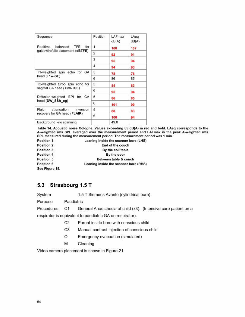
54
Sequence Position LAFmax
dB(A) LAeq
dB(A) 1 108 107 2 92 91 3 95 94
Realtime balanced TFE for guidewire/clip placement (sBTFE)
4 94 93 5 78 76 T1-weighted spin echo for GA
head (T1w-SE) 6 86 85 5 84 83 T2-weighted turbo spin echo for
sagittal GA head (T2w-TSE) 6 95 94 5 86 85 Diffusion-weighted EPI for GA
head (DW_SSh_og) 6 101 99 5 88 83 Fluid attenuation inversion
recovery for GA head (FLAIR) 6 100 94
Background -no scanning 49.0
Table 14. Acoustic noise Cologne. Values exceeding 85 dB(A) in red and bold. LAeq corresponds to the A-weighted rms SPL averaged over the measurement period and LAFmax is the peak A-weighted rms SPL measured during the measurement period. The measurement period was 1 min. Position 1: Leaning inside the scanner bore (LHS) Position 2: End of the couch Position 3: By the coil table Position 4: By the door Position 5: Between table & couch Position 6: Leaning inside the scanner bore (RHS) See Figure 15.
5.3 Strasbourg 1.5 T
System 1.5 T Siemens Avanto (cylindrical bore)
Purpose Paediatric
Procedures C1 General Anaesthesia of child (x3). (Intensive care patient on a
respirator is equivalent to paediatric GA on respirator).
C2 Parent inside bore with conscious child
C3 Manual contrast injection of conscious child
O Emergency evacuation (simulated)
M Cleaning
Video camera placement is shown in Figure 21.
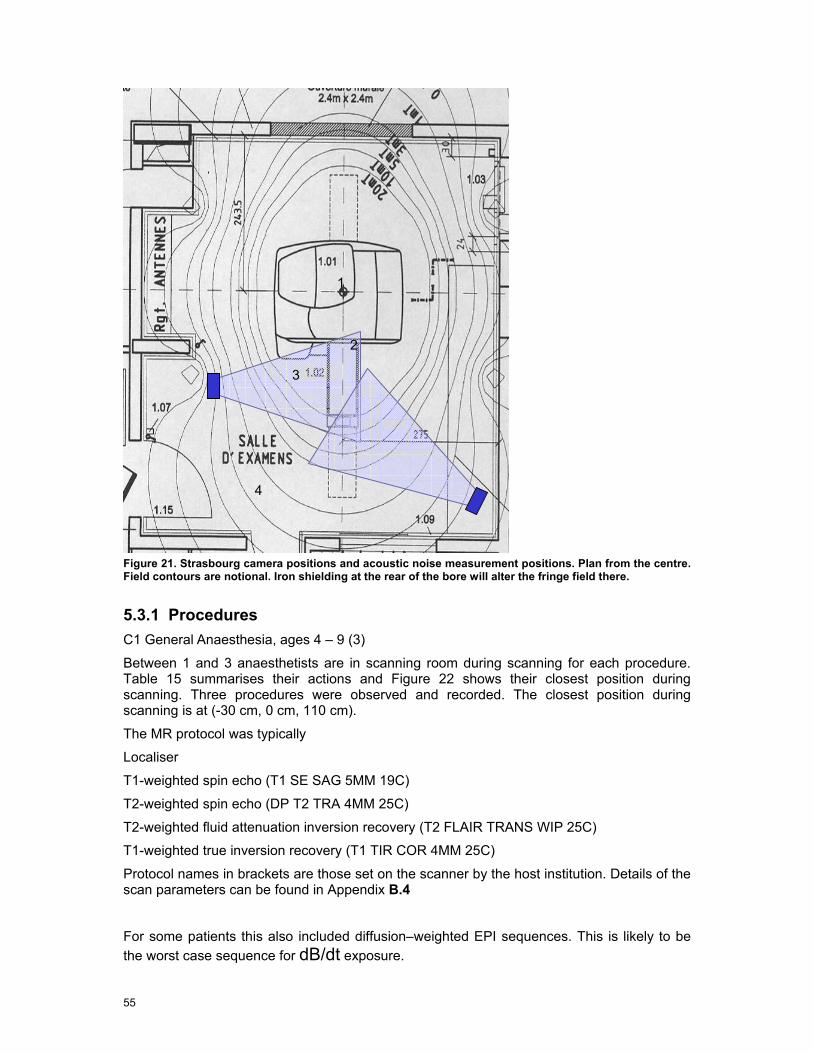
55
Figure 21. Strasbourg camera positions and acoustic noise measurement positions. Plan from the centre. Field contours are notional. Iron shielding at the rear of the bore will alter the fringe field there.
5.3.1 Procedures C1 General Anaesthesia, ages 4 – 9 (3)
Between 1 and 3 anaesthetists are in scanning room during scanning for each procedure. Table 15 summarises their actions and Figure 22 shows their closest position during scanning. Three procedures were observed and recorded. The closest position during scanning is at (-30 cm, 0 cm, 110 cm).
The MR protocol was typically
Localiser
T1-weighted spin echo (T1 SE SAG 5MM 19C)
T2-weighted spin echo (DP T2 TRA 4MM 25C)
T2-weighted fluid attenuation inversion recovery (T2 FLAIR TRANS WIP 25C)
T1-weighted true inversion recovery (T1 TIR COR 4MM 25C)
Protocol names in brackets are those set on the scanner by the host institution. Details of the scan parameters can be found in Appendix B.4
For some patients this also included diffusion–weighted EPI sequences. This is likely to be the worst case sequence for dB/dt exposure.
1
2
3
4
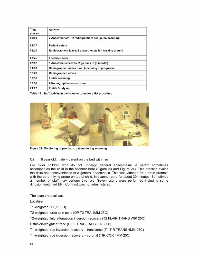
56
Time mm:ss
Activity
00:00 2 Anaesthetists + 2 radiographers set up, no scanning
02:37 Patient enters
03:20 Radiographers leave; 2 anaesthetists left walking around
03:45 Localiser scan
07:57 1 Anaesthetist leaves, 2 go back in (3 in total)
11:50 Radiographer enters room (scanning in progress)
12:28 Radiographer leaves
18:36 Finish scanning
19:50 2 Radiographers enter room
21:07 Finish & tidy up
Table 15. Staff activity in the scanner room for a GA procedure.
Figure 22. Monitoring of paediatric patient during scanning.
C2 8 year old, male – parent on the bed with him
For older children who do not undergo general anaesthesia, a parent sometimes accompanies the child in the scanner bore (Figure 23 and Figure 24). This practice avoids the risks and inconvenience of a general anaesthetic. This was videoed for a brain protocol with the parent lying prone on top of child, in scanner bore for about 30 minutes. Sometimes a member of staff may perform this role. Seven scans were performed including some diffusion-weighted EPI. Contrast was not administered.
The scan protocol was:
Localiser
T1-weighted 3D (T1 3D)
T2-weighted turbo spin echo (DP T2 TRA 4MM 25C)
T2-weighted fluid attenuation inversion recovery (T2 FLAIR TRANS WIP 25C)
Diffusion-weighted trace (DIFF TRACE ADC 0 A 3000)
T1-weighted true inversion recovery – transverse (T1 TIR TRANS 4MM 25C)
T1-weighted true inversion recovery – coronal (TIR COR 4MM 25C)
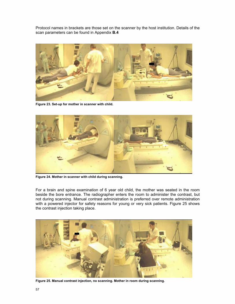
57
Protocol names in brackets are those set on the scanner by the host institution. Details of the scan parameters can be found in Appendix B.4
Figure 23. Set-up for mother in scanner with child.
Figure 24. Mother in scanner with child during scanning.
For a brain and spine examination of 6 year old child, the mother was seated in the room beside the bore entrance. The radiographer enters the room to administer the contrast, but not during scanning. Manual contrast administration is preferred over remote administration with a powered injector for safety reasons for young or very sick patients. Figure 25 shows the contrast injection taking place.
Figure 25. Manual contrast injection, no scanning. Mother in room during scanning.

58
O Emergency evacuation
The evacuation of a patient was simulated. Staff did not exceed the static field action value. No scanning takes place during this activity.
M Cleaning – simulated
The cleaner (non-MR person) in blues does general, regular cleaning (mopping the floor and dusting). The MR radiographer in whites does cleaning inside the bore, e.g. post infection cleaning. For this the radiographer leans into the bore. Both people go round the back of the scanner to clean (not seen in video).
5.3.2 Acoustic Noise Results for paediatric head examination scans are shown in Table 16. Positions are indicated in Figure 21. The average SPLs for staff are mainly below 85 dB(A). Hearing protection was not used.
Sequence Position LAFmax
dB(A) LAeq
dB(A) 1 81 79 2 77 76
T1-weighted spin echo (T1 SE SAG 1000 FLIP 100)
3 76 76 1 83 73 2 83 81
T2-weighted turbo spin echo (DP T2 TRA)
3 77 75 1 81 74 2 77 71
T2-weighted fluid attenuation inversion recovery (T2 FLAIR TRA WIP 25C)
3 78 71 1 88 86 2 87 85 3 88 86
Diffusion-weighted trace (DIFF TRACE ADC 0-1000)
4 85 83 1 84 83 2 79 77
T2-weighted constructive interference steady state (T2 CISS TRA CITERNES)
3 77 75
Table 16. Acoustic noise Strasbourg 1.5 T. Values exceeding 85 dB(A) in red and bold font. Position 1: Leaning inside the scanner bore Position 2: Standing next to the bore on the right hand side Position 3: Seated on the left hand side, slightly set-back from the bore & couch Position 4: By the control room door

59
5.4 Leuven 3.0T / 1.5 T
System 3.0 T Philips (cylindrical bore)
Purpose fMRI and neuro (mainly research, but some clinical)
Procedures C1 Clinical fMRI (tactile stimulus) 3.0 T
C3 General anaesthesia (children) 1.5 T
C2 Cardiac Stress test 1.5 T
M Cleaning 1.5 T
M Emergency evacuation
Procedures C2 and C3 were observed on the 1.5 T system where they are usually performed. In the future they may migrate to 3.0 T. The camera positions for each scanner are shown in Figure 26 and Figure 27. The 3.0 T scanner procedures were filmed using a different lens with a smaller view angle.
Figure 26. Leuven 3.0 T camera positions and acoustic noise measurement positions.
1 2 3

60
Figure 27. Leuven 1.5 T Camera positions and acoustic noise measurement positions
5.4.1 Procedures C1 fMRI sensory (3.0 T)
Functional MRI (fMRI) is performed on patients prior to brain surgery to allow surgeons to plan and to avoid damaging functionally important areas of the cerebral cortex. In the procedure observed the technician enters the room to apply a tactile stimulation to the patient’s hand during the fMRI scan (Figure 28). The technician is not present for any other scan. The fMRI scan lasted about 5 minutes. The technician’s movements are summarised in Figure 29 and Table 17. Two procedures were observed and recorded. The action value for the static field is exceeded. The maximum induced current from movement is given in Table 54. The gradient dB/dt exposures depend upon the image orientation, but exceed the relevant AV. The patient’s relative remained in the room for the whole examination.
3
1
2

61
Figure 28. Tactile stimulation during fMRI. Second person is a relative.
Time mm:ss
Activity
00:00 Radiographers position patient
09:38 Staff leave room and scan starts. Relative remains with patient
Survey Reference scan fMRI Stability check T2 scan fMRI 1 visual
26:50 Radiographer enters room for sensory paradigm Reference scan fMRI 2 sensory
32:40 Radiographer leaves room
34:36 Scan carries on Diffusion tensor imaging (DTI) Structural scan (MP-RAGE)
53:15 Patient is out
Table 17. Technician’s activity during fMRI examination.
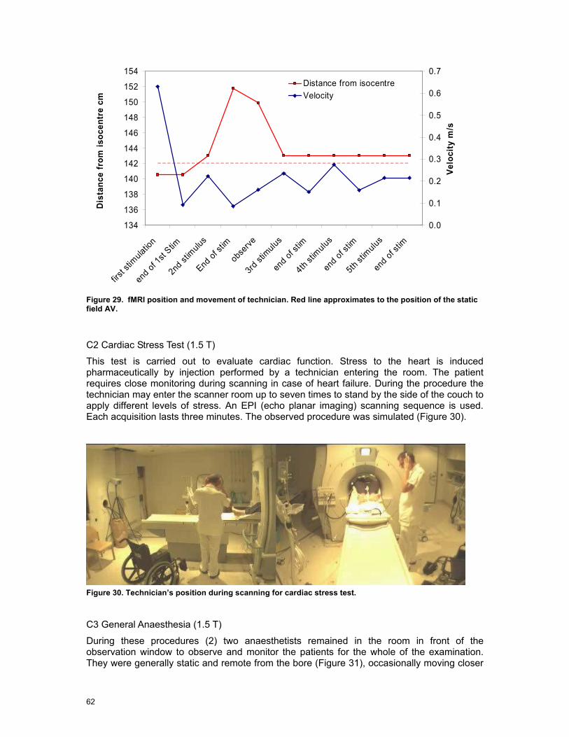
62
Figure 29. fMRI position and movement of technician. Red line approximates to the position of the static field AV.
C2 Cardiac Stress Test (1.5 T)
This test is carried out to evaluate cardiac function. Stress to the heart is induced pharmaceutically by injection performed by a technician entering the room. The patient requires close monitoring during scanning in case of heart failure. During the procedure the technician may enter the scanner room up to seven times to stand by the side of the couch to apply different levels of stress. An EPI (echo planar imaging) scanning sequence is used. Each acquisition lasts three minutes. The observed procedure was simulated (Figure 30).
Figure 30. Technician’s position during scanning for cardiac stress test.
C3 General Anaesthesia (1.5 T)
During these procedures (2) two anaesthetists remained in the room in front of the observation window to observe and monitor the patients for the whole of the examination. They were generally static and remote from the bore (Figure 31), occasionally moving closer
134
136
138
140
142
144
146
148
150
152
154
first s
timulat
ion
end of 1
st Stim
2nd st
imulu
s
End of st
im
observ
e
3rd st
imulus
end o
f stim
4th stim
ulus
end of s
tim
5th st
imulu
s
end of s
tim
Dis
tanc
e fr
om is
ocen
tre
cm
0.0
0.1
0.2
0.3
0.4
0.5
0.6
0.7
Velo
city
m/s
Distance from isocentreVelocity
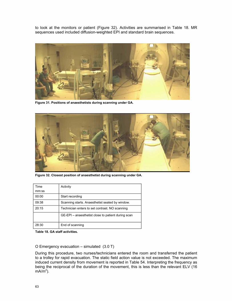
63
to look at the monitors or patient (Figure 32). Activities are summarised in Table 18. MR sequences used included diffusion-weighted EPI and standard brain sequences.
Figure 31. Positions of anaesthetists during scanning under GA.
Figure 32. Closest position of anaesthetist during scanning under GA.
Time mm:ss
Activity
00:00 Start recording
09:38 Scanning starts. Anaesthetist seated by window.
20:15 Technician enters to set contrast. NO scanning
GE-EPI – anaesthetist close to patient during scan
28:30 End of scanning
Table 18. GA staff activities.
O Emergency evacuation – simulated (3.0 T)
During this procedure, two nurses/technicians entered the room and transferred the patient to a trolley for rapid evacuation. The static field action value is not exceeded. The maximum induced current density from movement is reported in Table 54. Interpreting the frequency as being the reciprocal of the duration of the movement, this is less than the relevant ELV (16 mA/m2).

64
M2 Cleaning (1.5 T)
Two technicians entered the scanner room. One of them mounted the patient table and was moved into the bore to enable cleaning (Figure 33). This would be required after scanning an infectious patient or in the case of a patient vomiting (contrast reaction) or a blood spillage following an injection or biopsy (not performed here).
Figure 33. Cleaning the inside of the bore.
5.4.2 Acoustic Noise Acoustic noise data are shown in Table 19 and Table 20 for the positions defined in Figure 26 and Figure 27.
Sequence (3.0 T) Position LAFmax
dB(A) LAeq
dB(A)
1 103 102 2 101 98
Functional MRI echo planar imaging for tactile stimulation (fMRI-EPI)
3 111 111 Table 19. Acoustic noise Leuven 3.0 T. Values exceeding 85 dB(a) in red and bold font Position 1: At scanner bore entrance Position 2: End of the couch Position 3: By patient’s ear (near isocentre)

65
Sequence (1.5 T) Position LAFmax
dB(A) LAeq
dB(A) 1 98 97 2 90 88
Balanced turbo field echo for cardiac (bTFE)
3 107 105 1 77 76 Diffusion-weighted echo planar
imaging for GA head (DWI EPI) 2 81 80 1 94 93 Perfusion EPI for cardiac stress
test 2 86 86
Table 20. Acoustic noise Leuven 1.5 T. Values exceeding 85 dB(A) in red and bold font Position 1: Stress technician – side of couch Position 2: Anaesthetist - chair Position 3: By patient’s ear (near isocentre)
5.5 Nottingham 7.0 T
System 7.0 T Philips (cylindrical bore)
Purpose High field research
Procedures C1 Manual contrast injection
C2 Adjustment of EEG electrodes
C3 Emergency evacuation
Figure 34. Camera positions, Nottingham. Rear of magnet for EEG set-up, front for manual contrast. Field plot from Dr. P. Glover, University of Nottingham. Acoustic noise measurement positions are shown in red and bold font.
1
2
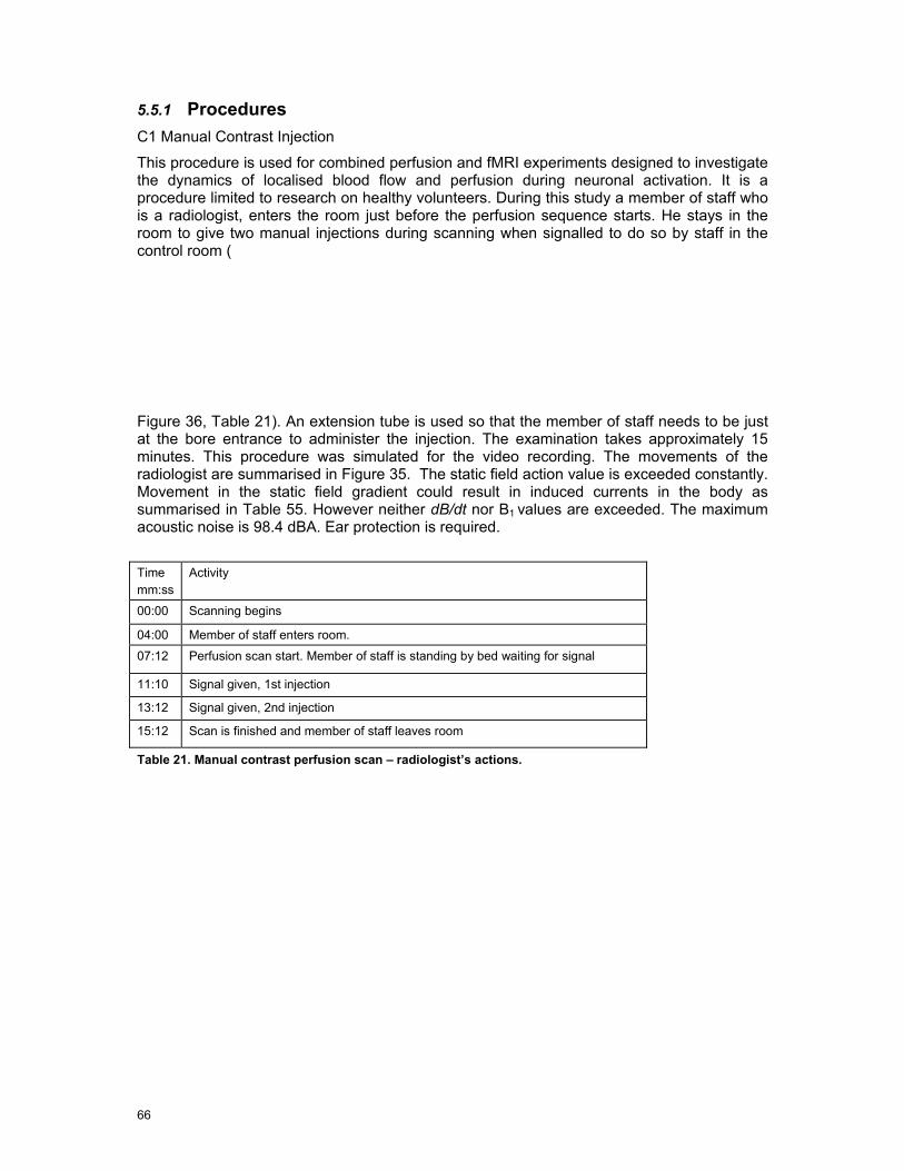
66
5.5.1 Procedures
C1 Manual Contrast Injection
This procedure is used for combined perfusion and fMRI experiments designed to investigate the dynamics of localised blood flow and perfusion during neuronal activation. It is a procedure limited to research on healthy volunteers. During this study a member of staff who is a radiologist, enters the room just before the perfusion sequence starts. He stays in the room to give two manual injections during scanning when signalled to do so by staff in the control room (
Figure 36, Table 21). An extension tube is used so that the member of staff needs to be just at the bore entrance to administer the injection. The examination takes approximately 15 minutes. This procedure was simulated for the video recording. The movements of the radiologist are summarised in Figure 35. The static field action value is exceeded constantly. Movement in the static field gradient could result in induced currents in the body as summarised in Table 55. However neither dB/dt nor B1
values are exceeded. The maximum acoustic noise is 98.4 dBA. Ear protection is required.
Time mm:ss
Activity
00:00 Scanning begins
04:00 Member of staff enters room.
07:12 Perfusion scan start. Member of staff is standing by bed waiting for signal
11:10 Signal given, 1st injection
13:12 Signal given, 2nd injection
15:12 Scan is finished and member of staff leaves room
Table 21. Manual contrast perfusion scan – radiologist’s actions.
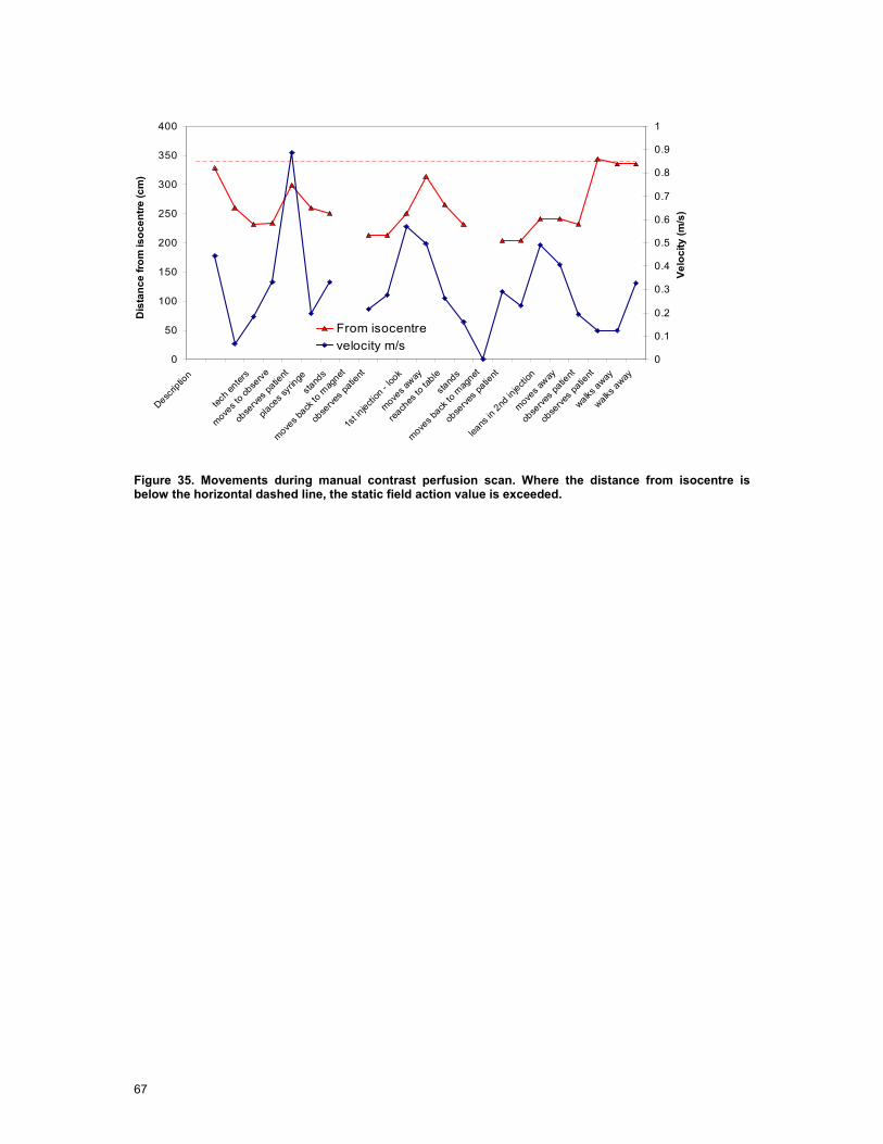
67
Figure 35. Movements during manual contrast perfusion scan. Where the distance from isocentre is below the horizontal dashed line, the static field action value is exceeded.
0
50
100
150
200
250
300
350
400
Descrip
tion
tech e
nters
moves t
o obse
rve
obse
rves p
atient
place
s syri
nge
stand
s
moves b
ack to
mag
net
obse
rves p
atient
1st in
jection
- loo
k
moves a
way
reach
es to
table
stand
s
moves b
ack to
mag
net
obse
rves p
atient
leans
in 2nd
injecti
on
moves a
way
obse
rves p
atient
obse
rves p
atient
walks away
walks away
Dis
tanc
e fro
m is
ocen
tre (c
m)
0
0.1
0.2
0.3
0.4
0.5
0.6
0.7
0.8
0.9
1
Velo
city
(m/s
)
From isocentrevelocity m/s
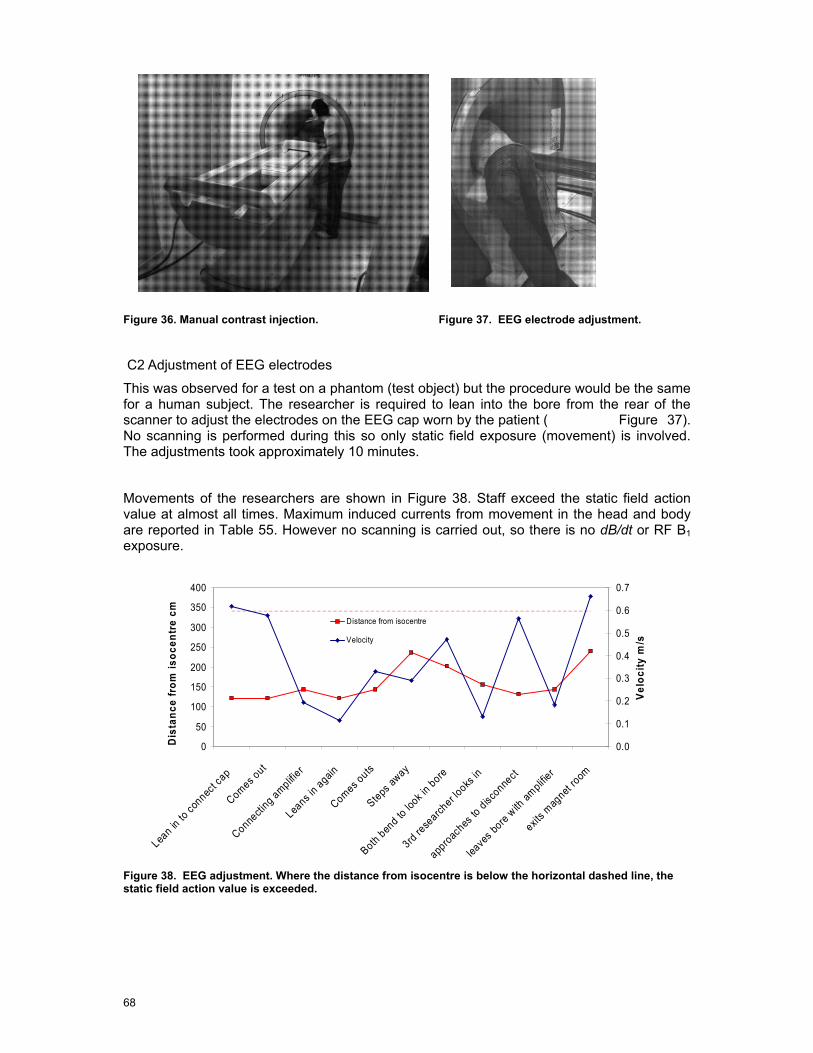
68
Figure 36. Manual contrast injection. Figure 37. EEG electrode adjustment.
C2 Adjustment of EEG electrodes
This was observed for a test on a phantom (test object) but the procedure would be the same for a human subject. The researcher is required to lean into the bore from the rear of the scanner to adjust the electrodes on the EEG cap worn by the patient ( Figure 37). No scanning is performed during this so only static field exposure (movement) is involved. The adjustments took approximately 10 minutes.
Movements of the researchers are shown in Figure 38. Staff exceed the static field action value at almost all times. Maximum induced currents from movement in the head and body are reported in Table 55. However no scanning is carried out, so there is no dB/dt or RF B1 exposure.
Figure 38. EEG adjustment. Where the distance from isocentre is below the horizontal dashed line, the static field action value is exceeded.
0
50
100
150
200
250
300
350
400
Lean in
to co
nnect c
ap
Comes out
Connecti
ng amplifie
r
Leans i
n again
Comes outs
Steps aw
ay
Both ben
d to lo
ok in bore
3rd rese
archer lo
oks in
approac
hes to
disconne
ct
leave
s bore w
ith am
plifier
exits m
agnet
room
Dis
tanc
e fr
om is
ocen
tre
cm
0.0
0.1
0.2
0.3
0.4
0.5
0.6
0.7
Velo
city
m/s
Distance from isocentre
Velocity
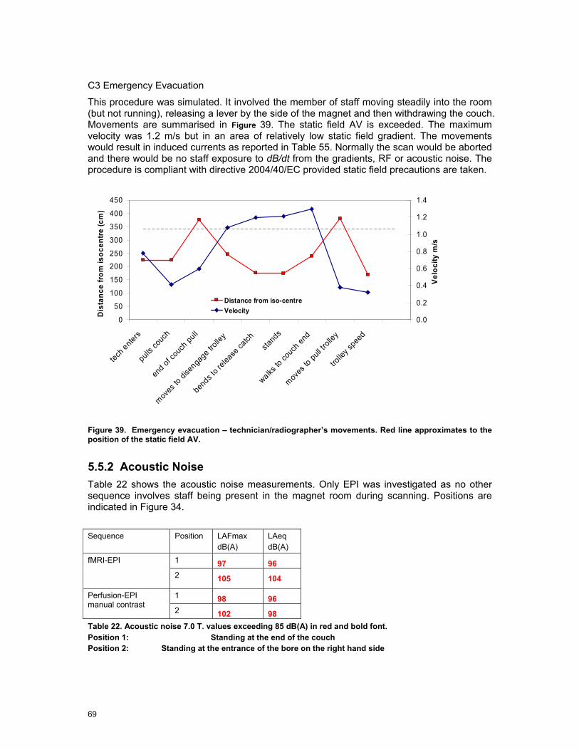
69
C3 Emergency Evacuation
This procedure was simulated. It involved the member of staff moving steadily into the room (but not running), releasing a lever by the side of the magnet and then withdrawing the couch. Movements are summarised in Figure 39. The static field AV is exceeded. The maximum velocity was 1.2 m/s but in an area of relatively low static field gradient. The movements would result in induced currents as reported in Table 55. Normally the scan would be aborted and there would be no staff exposure to dB/dt from the gradients, RF or acoustic noise. The procedure is compliant with directive 2004/40/EC provided static field precautions are taken.
Figure 39. Emergency evacuation – technician/radiographer’s movements. Red line approximates to the position of the static field AV.
5.5.2 Acoustic Noise Table 22 shows the acoustic noise measurements. Only EPI was investigated as no other sequence involves staff being present in the magnet room during scanning. Positions are indicated in Figure 34.
Sequence Position LAFmax
dB(A) LAeq
dB(A) 1 97 96 fMRI-EPI
2 105 104
1 98 96 Perfusion-EPI manual contrast
2 102 98 Table 22. Acoustic noise 7.0 T. values exceeding 85 dB(A) in red and bold font. Position 1: Standing at the end of the couch Position 2: Standing at the entrance of the bore on the right hand side
0
50
100
150
200
250
300
350
400
450
tech ente
rs
pulls c
ouch
end of
couc
h pull
moves
to di
senga
ge trolle
y
bends t
o relea
se ca
tchsta
nds
walks to
couch
end
moves t
o pull
trolle
y
trolle
y spee
d
Dis
tanc
e fro
m is
ocen
tre (c
m)
0.0
0.2
0.4
0.6
0.8
1.0
1.2
1.4
Velo
city
m/s
Distance from iso-centreVelocity
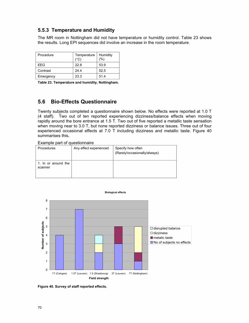
70
5.5.3 Temperature and Humidity The MR room in Nottingham did not have temperature or humidity control. Table 23 shows the results. Long EPI sequences did involve an increase in the room temperature.
Procedure Temperature
(°C) Humidity (%)
EEG 22.8 53.9 Contrast 24.4 52.5 Emergency 23.3 51.4
Table 23. Temperature and humidity, Nottingham.
5.6 Bio-Effects Questionnaire
Twenty subjects completed a questionnaire shown below. No effects were reported at 1.0 T (4 staff). Two out of ten reported experiencing dizziness/balance effects when moving rapidly around the bore entrance at 1.5 T. Two out of five reported a metallic taste sensation when moving near to 3.0 T, but none reported dizziness or balance issues. Three out of four experienced occasional effects at 7.0 T including dizziness and metallic taste. Figure 40 summarises this. Example part of questionnaire Procedures Any effect experienced
Specify how often (Rarely/occasionally/always)
1. In or around the scanner
Biological effects
0
1
2
3
4
5
6
7
8
1T (Cologne) 1.5T (Leuven) 1.5 (Strasbourg) 3T (Leuven) 7T (Nottingham)
Field strength
Num
ber o
f sub
ject
s
disrupted balancedizzinessmetalic tasteNo of subjects no effects
Figure 40. Survey of staff reported effects.

71
5.7 Consultation with Radiological and Clinical Experts
The radiological and clinical experts were shown videos of the procedures which involved significant or potential dB/dt and RF exposure of staff. These were: clip insertion and breast biopsy (Cologne), fMRI, GA and cardiac stress (Leuven), child with parent and GA (Strasbourg).
There was a variety of opinion about the GA procedures concerning whether staff need to be in the MR room for the safety of the patient. Some MR centres may not be suitably equipped with appropriate access for the monitoring to be done remotely. However, sedation does require a person in the MR room. Scanner door interlocks may prevent staff entering the room temporarily during a procedure.
The biopsy and clip insertions were considered normal practice. EMF exposure is unavoidable for the real-time guided clip insertion.
The parent in the scanner with the child was not considered as normal practice. Support is usually given by the carer sitting by the bore entrance.
Additionally they were asked about cleaning the magnet and for other clinical procedures potentially affected by directive 2004/40/EC. These included: cardiac and interventional radiology, post-mortem biopsies, MR guided focussed ultrasound and laser ablation.
The completed questionnaires are contained in Appendix B.
Acknowledgements
We wish to acknowledge the four MRI centres and their staff and patients for access to their MRI systems to carry out his project and for their contributions to it. In particular we thank Dr. Axel Gossmann, M. Daniel Vetter, Prof. Stefan Sunaert, Prof. Guy Marchal, Mr. Stefan Ghysels, Prof. Paul van Hecke, Dr. Ronald Peeters, Dr. Paul Glover, Mr. Andrew Peters and Prof. Penny Gowland. We also thank Hans Engels, Rutger Bakker, Urs Sturzenegger (Philips), Georg Frese, Marc Beckmann (Siemens), the panel of clinical experts: Prof. Wadyslaw Gedroyc, Dr. Andrew Taylor and Dr. Adam Waldman, and the encouragement and support of M. Georges Herbillon, the Monitoring Group and the European Society of Radiology.

6 Assessment of Incident Fields
This chapter reports the outcome of the workpackage that was concerned with the measurement campaign at the four MRI sites and in particular involves the following elements:
• A description of the measurement equipment and data acquisition.
• The measurement procedure.
• Performed field measurements
• Measurement reporting (including evaluation)
Throughout Section 6 reference is made to the Physical Agents Directive 2004/40/EC [13] and the ICNIRP guidelines for exposure to non-ionising radiation [10] with particular note made to the analysis of the non-sinusoidal gradient fields and their interpretation within the ICNIRP framework [11].
6.1 Methods
6.1.1 Background The goal of the project is to map the static, gradient and RF fields in the vicinity of an MRI machine on a fixed grid. The probe positioning was manual and supported mechanically. The position was identified by an optical indicator (projected image on a screen inside the scanner room) in order to minimize erroneous measurement location selection. Taking the actual reading was triggered by the measurement operator (a trigger optically connected to the PXI data acquisition system was used)
6.1.2 Overview The measurement software was implemented in Labview and supported the data acquisition for measurements of the static, gradient and RF fields in the MRI environments. Additionally, a projector based measurement location indicator was provided to ensure measurement of the correct location and no loss of synchronisation.
Instruments
• B0 Static Field – Metrolab THM7025
• Gradient Field – Narda ELT-400 + National Instruments PXI
• B1 RF Field – EASY4MRI
Positioning
• Hybrid mechanical – optical positioning system with 300 mm grid resolution
Data Collection
• Data was collected for areas exceeding the action values using a Labview based data acquisition system.
• For the static B0 field the magnitude was recorded at each position

73
• For gradient fields the full waveform for the 3 orthogonal sensors was collected for excitation of x, y and z gradient coils at each position
• For B1 RF fields component values E and H fields will be recorded along with a reference probe as close to the isocentre as allowed by the MRI phantom.
6.2 Instrumentation
6.2.1 B-field The mapping of the static fields has been performed with a 3-axis Hall Teslameter THM 7025 of Metrolab, Geneva, Switzerland (Figure 41). The specifications of the instrument are summarized in Table 24.
Figure 41. Metrolab 3-axis Hall Teslameter THM 7025 (source: http://www.metrolab.com)
Ranges 20 mT, 200 mT, 2 T Resolution 0.01 mT. 0.1 mT, 1 mT Display 3.5 digit Reading B or Bz (Bx, By, Bz, B via RS232) Uncertainty 2% Gain Temp. Coefficient 0.05 %/K Update rate 0.4s Operating Temp. 0 – 40 deg C Output RS232 Instrument size 160x80x30 mm Sensor size 12x12x100 mm Weight 250 g
Table 24 Metrolab 3-axis Hall Teslameter THM 7025 - Specifications
6.2.2 Gradient Field The gradient field distribution has been mapped using the Narda-STS ELT400 low frequency 3-axis magnetic field meters available. The ELT400 provides an input filter shaped in response to the exposure limits of the ICNIRP guideline. This feature has been used to work out the required field mapping space. The ELT400 also provides an analog voltage output

74
proportional to the B-field measured by the x,y,z-sensors. This feature has been used to obtain the time-domain signal from the x,y,z-gradient coils for the clinical sequences and the test sequence.
Figure 42. Narda ELT400 3-axis low frequency magnetic field meter (source: http://www.narda-sts.de/)
Frequency Range 1 Hz -400 kHz, 10 Hz – 400 kHz, 30 Hz-400 kHz Uncertainty 4% (5Hz-120kHz) E-field response <187.5 nT @ f, 2 kHz, 100 V/m Standard Mode: Mode ICNIRP BGV B11 EN 50366 Range Low High Low High Low High Overload limit 160% 1600% 160% 1600% 160% 1600% Noise 1% 5% 0.4% 2% 0.4% 2% Resolution 0.001% (range low) Field Meter Mode: Mode 320 uT 80 mT
Range Low High Low High
Overload limit 32 uT 320 uT 8 mT 80 mT
Noise 60 nT 320 nT 10 uT 80 uT
Resolution 1 nT (Range: low) Output: Analog scope output Three channel x, y, z Analog output level 800 mV/(overload limit) Remote Control: RS 232 General: Temperature range -10 … 50 deg C Humidity range < 95% (@ 30 deg C) Base unit – size 180x100x55 mm Probe – size 290 x 125 (∅) mm Probe Extension Cable 1 m
Table 25. ELT400 Specification.
The time-domain x,y and z-signals from the ELT400 were coherently sampled using a National Instrument PXI system equipped with a PXI-6115 4-channel 10 MSamples/s synchronous sampling module. The setup enables the sampling of the waveforms with a reasonably high sampling rate and direct streaming of the sampled data to a hard disk over the duration of a full MRI scan. Additionally, the PXI system was equipped with a PXI-6514
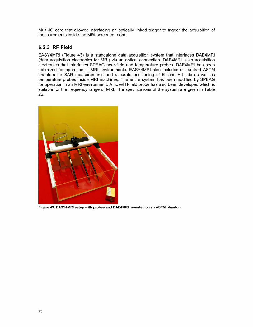
75
Multi-IO card that allowed interfacing an optically linked trigger to trigger the acquisition of measurements inside the MRI-screened room.
6.2.3 RF Field EASY4MRI (Figure 43) is a standalone data acquisition system that interfaces DAE4MRI (data acquisition electronics for MRI) via an optical connection. DAE4MRI is an acquisition electronics that interfaces SPEAG near-field and temperature probes. DAE4MRI has been optimized for operation in MRI environments. EASY4MRI also includes a standard ASTM phantom for SAR measurements and accurate positioning of E- and H-fields as well as temperature probes inside MRI machines. The entire system has been modified by SPEAG for operation in an MRI environment. A novel H-field probe has also been developed which is suitable for the frequency range of MRI. The specifications of the system are given in Table 26.
Figure 43. EASY4MRI setup with probes and DAE4MRI mounted on an ASTM phantom

76
E-field probe: SPEAG ER3DV6 Frequency range 40 - 6000 MHz Dynamic range 1 - 1000 V/m Spatial resolution < 7 mm Directivity error < ±0.3 dB H-field probe: SPEAG H3DV7 Frequency range 40 - 3000 MHz Dynamic range 0.01 A/m to 10 A/m @128 MHz Spatial resolution < 4 mm Directivity error < ±0.2 dB Data Acquisition Electronics SPEAG DAE4MRI Input range -100 … 300 mV Power Lithium Polymer rechargeable battery Output Optical Noise <7 uV Sampling rate 128 us Data Logger / Field Monitor SPEAG EASY4MRI DAE4MRI inputs 4x optical DAE power output 4x Interfaces: RS 232 , ETHERNET, USB, Floppy Drive Modes Real-time monitoring, data recording, remote data acquisition Sampling rate 10 ms to hours
Table 26. EASY4MRI specifications
The electromagnetic immunity of the EASY4MRI measurement system was evaluated in 1.5T and a 3T MRI machines. The results are shown in Table 27. Data Acquisition
Electronics H-Field E-field
Type DAEMRI H3DV7 ER3DV6 Acceleration <0.1 G/T 0.01 G/T <0.01 G/T Noise (laboratory conditions) <7 uV <10 mA/m <1 V/m Noise (1.5T) static <10 uV <10 mA/m <1.2 V/m Noise (3T) static <10 uV <10 mA/m <1.2 V/m Noise (1.5T) static + gradient <10 uV <10 mA/m <1.2 V/m Noise (3T) static + gradient <20 uV <17 mA/m <1.7 V/m Noise (1.5T) static + gradient + RF <40 uV n.a. n.a. Noise (3T) static + gradient + RF <40 uV n.a. n.a.
Table 27. EASY4MRI MRI-EMI Results
6.2.4 Data Acquisition Software System The manual field mapping is supported by a data acquisition software application (Figure 44) specifically designed to meet the requirement of mapping large volumes inside MRI screened rooms. The software interfaces the static magnetic, low-frequency magnetic and RF electromagnetic measurement equipment as well as an optically linked measurement trigger,

77
including setting up, triggering and data acquisition (Figure 45). The graphical user interface has been designed to guide and support the measurement personnel inside the MRI screened room and to give feedback on acquired data. Therefore the control display can be projected through a window inside the MRI screened room (Figure 46).
Figure 44. A screenshot from the EX-MRI-Occ data acquisition control software

78
Figure 45. Control Chart of the EX-MRI-Occ data acquisition software
Figure 46. Graphical user interface projected inside the MRI screened room.
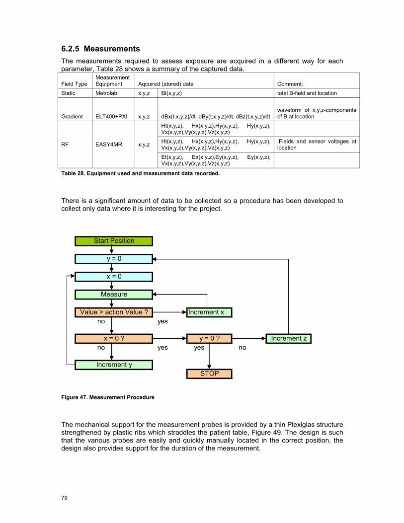
79
6.2.5 Measurements The measurements required to assess exposure are acquired in a different way for each parameter, Table 28 shows a summary of the captured data.
Field Type Measurement Equipment Aqcuired (stored) data Comment:
Static Metrolab x,y,z Bt(x,y,z) total B-field and location
Gradient ELT400+PXI x,y,z dBx(t,x,y,z)/dt ,dBy(t,x,y,z)/dt, dBz(t,x,y,z)/dt
waveform of x,y,z-components of B at location
Ht(x,y,z), Hx(x,y,z),Hy(x,y,z), Hy(x,y,z), Vx(x,y,z),Vy(x,y,z),Vz(x,y,z) Ht(x,y,z), Hx(x,y,z),Hy(x,y,z), Hy(x,y,z), Vx(x,y,z),Vy(x,y,z),Vz(x,y,z)
Fields and sensor voltages at location RF EASY4MRI x,y,z
Et(x,y,z), Ex(x,y,z),Ey(x,y,z), Ey(x,y,z), Vx(x,y,z),Vy(x,y,z),Vz(x,y,z)
Table 28. Equipment used and measurement data recorded.
There is a significant amount of data to be collected so a procedure has been developed to collect only data where it is interesting for the project.
Start Position
y = 0
x = 0
Measure
Value > action Value ? Increment x no yes
x = 0 ? y = 0 ? Increment z no yes yes no
Increment ySTOP
Figure 47. Measurement Procedure
The mechanical support for the measurement probes is provided by a thin Plexiglas structure strengthened by plastic ribs which straddles the patient table, Figure 49. The design is such that the various probes are easily and quickly manually located in the correct position, the design also provides support for the duration of the measurement.

80
6.3 Measurement Procedure
The measurement of occupational exposure has three elements:
• Static magnetic field exposure
• Gradient magnetic field exposure
• RF electromagnetic field exposure
All measurements were performed on two measurement grids. These grids were a single plane designed for operation outside the bore of the magnet, and a smaller sub grid for inside the bore. In addition a range of supplementary measurements performed on the flared surfaces at the end of the bore.
NOTE that different manufacturers use different coordinate systems to describe their machines, even machines from the same manufacturer have different coordinate systems depending on the static field direction. Therefore to ensure consistency and clarity the definition of coordinates as shown in Figure 48 are used throughout. This is also the case for the open MRI, Z is aligned along the bed. The alignment of the ELT400 gradient field probe axes is also in accordance with Figure 48.
Y
X
Z
Figure 48. Coordinate system used throughout all measurements and analysis
6.3.1 Measurement Preparation The scanner bed is placed in its nominal ‘out’ position and the point that will be the isocentre when inserted marked with tape. A grid that will allow the in bore measurement to be placed at either 10 cm or 15 cm intervals was marked on the table with removable tape (the spacing was based on a combination of gradient and static field magnitudes, the higher the rate of change, the smaller the grid)
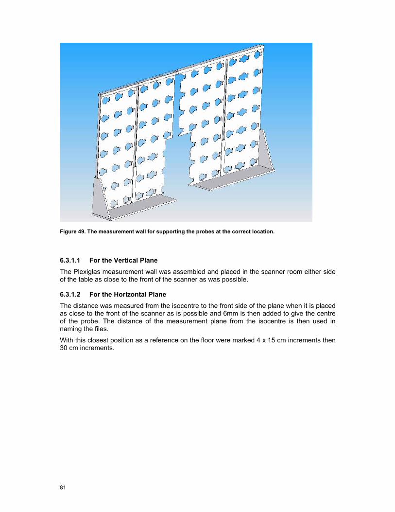
81
Figure 49. The measurement wall for supporting the probes at the correct location.
6.3.1.1 For the Vertical Plane The Plexiglas measurement wall was assembled and placed in the scanner room either side of the table as close to the front of the scanner as was possible.
6.3.1.2 For the Horizontal Plane The distance was measured from the isocentre to the front side of the plane when it is placed as close to the front of the scanner as is possible and 6mm is then added to give the centre of the probe. The distance of the measurement plane from the isocentre is then used in naming the files.
With this closest position as a reference on the floor were marked 4 x 15 cm increments then 30 cm increments.
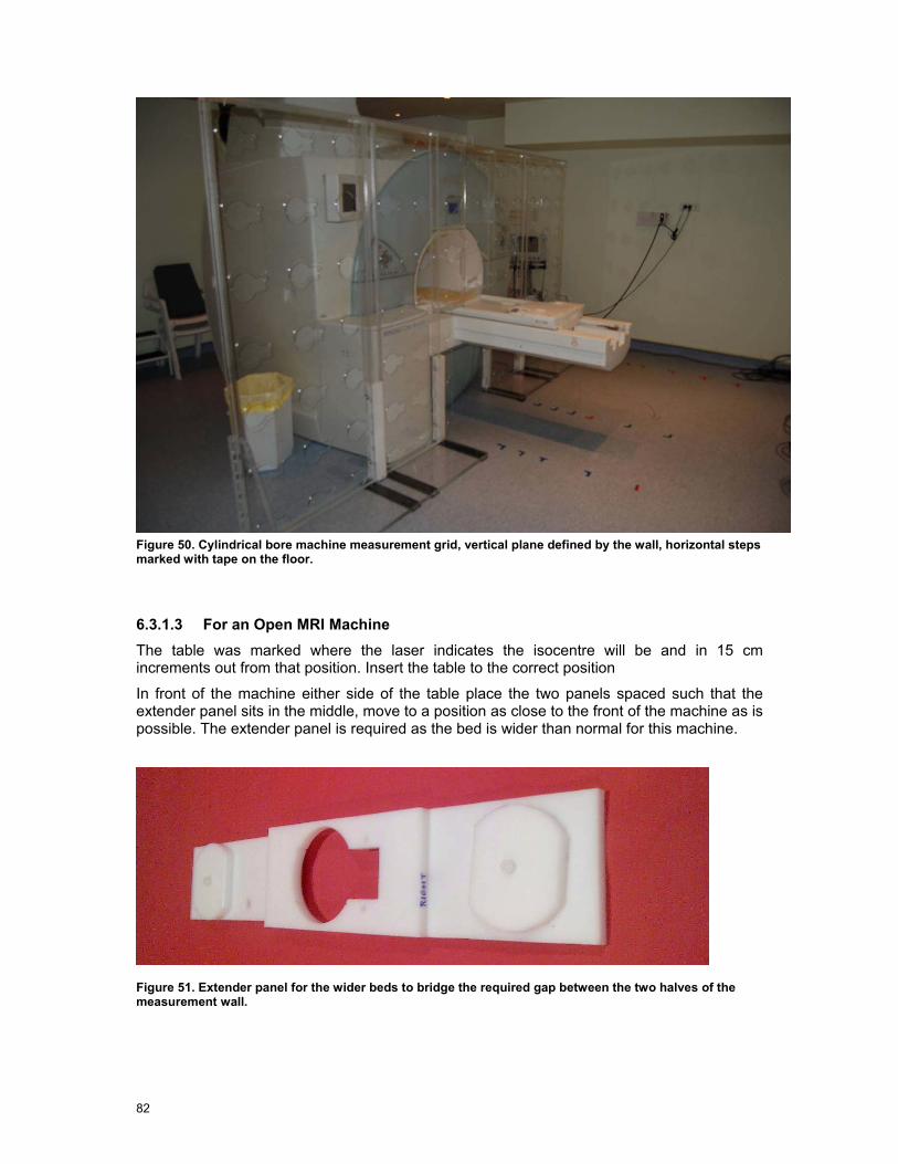
82
Figure 50. Cylindrical bore machine measurement grid, vertical plane defined by the wall, horizontal steps marked with tape on the floor.
6.3.1.3 For an Open MRI Machine The table was marked where the laser indicates the isocentre will be and in 15 cm increments out from that position. Insert the table to the correct position
In front of the machine either side of the table place the two panels spaced such that the extender panel sits in the middle, move to a position as close to the front of the machine as is possible. The extender panel is required as the bed is wider than normal for this machine.
Figure 51. Extender panel for the wider beds to bridge the required gap between the two halves of the measurement wall.

83
6.3.1.4 For the Vertical Plane The plexiglass measurement wall was assembled and placed either side of the table as close to the front of the scanner as was possible.
6.3.1.5 For the Horizontal Plane The distance of the isocentre to the front side of the plane measured and 6mm added, this is the distance of the measurement plane from the isocentre and was used in naming the files.
Mark on the floor 4 x 15 cm increments then 30 cm increments.
Figure 52. Open MRI measurement grid concept, outline drawing courtesy of Philips
6.3.2 Measurement Procedure For each position of the measurement grids three individual measurements must be made, best done as follows, whole vertical grid for static and gradient, move grid then perform the RF measurements (30cm behind the plane of the grid).
6.3.2.1 Static Field The static field was measured out to 20 mT, the distance depends on magnet type and active shielding but primarily on nominal static field strength. A brief survey was done to check the extent of the measurement area to limit the measurement time.
6.3.2.2 RF Field The RF field decays very rapidly and was measured down to 10dB below the action values, which are 61 V/m and 0.16 A/m for E and H field respectively. The -10 dB values are 19.3 V/m and 0.05 A/m respectively.
6.3.2.3 Gradient Field The gradient field measurement was more complex for the following reasons; there are 4 possible ranges of operation, we needed to note which was used at each point. When placing the probe, movement through the static field of the probe and the connecting cable also influence the measurement therefore it was important to watch the display and see when it had settled down to a constant value before triggering the measurement.
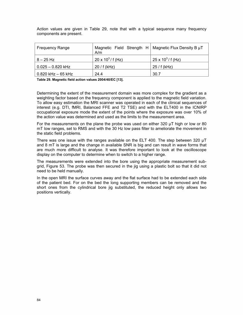
84
Action values are given in Table 29, note that with a typical sequence many frequency components are present.
Frequency Range Magnetic Field Strength H A/m
Magnetic Flux Density B µT
8 – 25 Hz 20 x 103 / f (Hz) 25 x 103 / f (Hz)
0.025 – 0.820 kHz 20 / f (kHz) 25 / f (kHz)
0.820 kHz – 65 kHz 24.4 30.7 Table 29. Magnetic field action values 2004/40/EC [13].
Determining the extent of the measurement domain was more complex for the gradient as a weighting factor based on the frequency component is applied to the magnetic field variation. To allow easy estimation the MRI scanner was operated in each of the clinical sequences of interest (e.g. DTI, fMRI, Balanced FFE and T2 TSE) and with the ELT400 in the ICNIRP occupational exposure mode the extent of the points where the exposure was over 10% of the action value was determined and used as the limits to the measurement area.
For the measurements on the plane the probe was used on either 320 µT high or low or 80 mT low ranges, set to RMS and with the 30 Hz low pass filter to ameliorate the movement in the static field problems.
There was one issue with the ranges available on the ELT 400. The step between 320 µT and 8 mT is large and the change in available SNR is big and can result in wave forms that are much more difficult to analyse. It was therefore important to look at the oscilloscope display on the computer to determine when to switch to a higher range.
The measurements were extended into the bore using the appropriate measurement sub-grid, Figure 53. The probe was then secured in the jig using a plastic bolt so that it did not need to be held manually.
In the open MRI the surface curves away and the flat surface had to be extended each side of the patient bed. For on the bed the long supporting members can be removed and the short ones from the cylindrical bore jig substituted, the reduced height only allows two positions vertically.
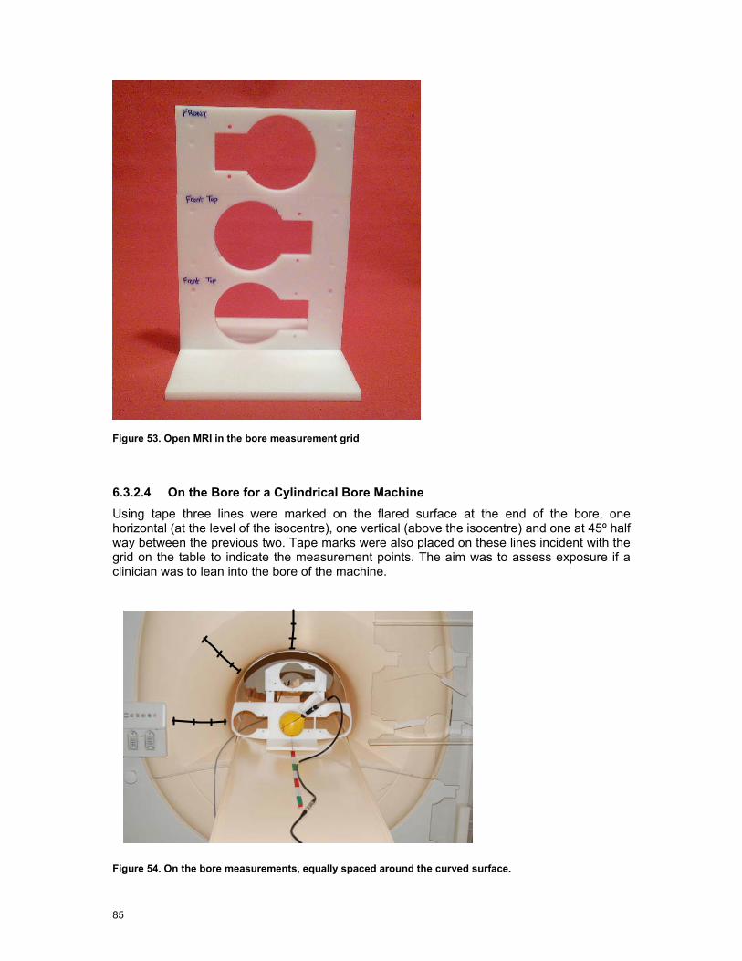
85
Figure 53. Open MRI in the bore measurement grid
6.3.2.4 On the Bore for a Cylindrical Bore Machine Using tape three lines were marked on the flared surface at the end of the bore, one horizontal (at the level of the isocentre), one vertical (above the isocentre) and one at 45º half way between the previous two. Tape marks were also placed on these lines incident with the grid on the table to indicate the measurement points. The aim was to assess exposure if a clinician was to lean into the bore of the machine.
Figure 54. On the bore measurements, equally spaced around the curved surface.

86
6.3.2.5 On the Bore for the Panorama Machine Using tape three lines were marked on the curved surface to the side of the patient bed, one on the Z axis, one on the X axis and one at 45º half way between the previous two. Equidistant tape marks were placed on these lines to form a grid for the measurements. The aim was to assess exposure if a clinician was to lean into the bore of the machine.
Figure 55. On the bore measurements in the open MRI
6.3.3 Clinical Sequence Measurement Measurement of the selected clinical sequences was done over a 5 second period with a sample rate of 50 k samples/sec. In the cylindrical bore machines this was done at a position on bore-site just in front of the machine and a position shifted right by 30 cm and up by 30 cm.
Figure 56. Conventional MRI in the Bore measurement grid

87
Figure 57. Static field probe secured in the measurement grid using M8 plastic bolt
Figure 58. Gradient field probe secured in the bore measurement grid
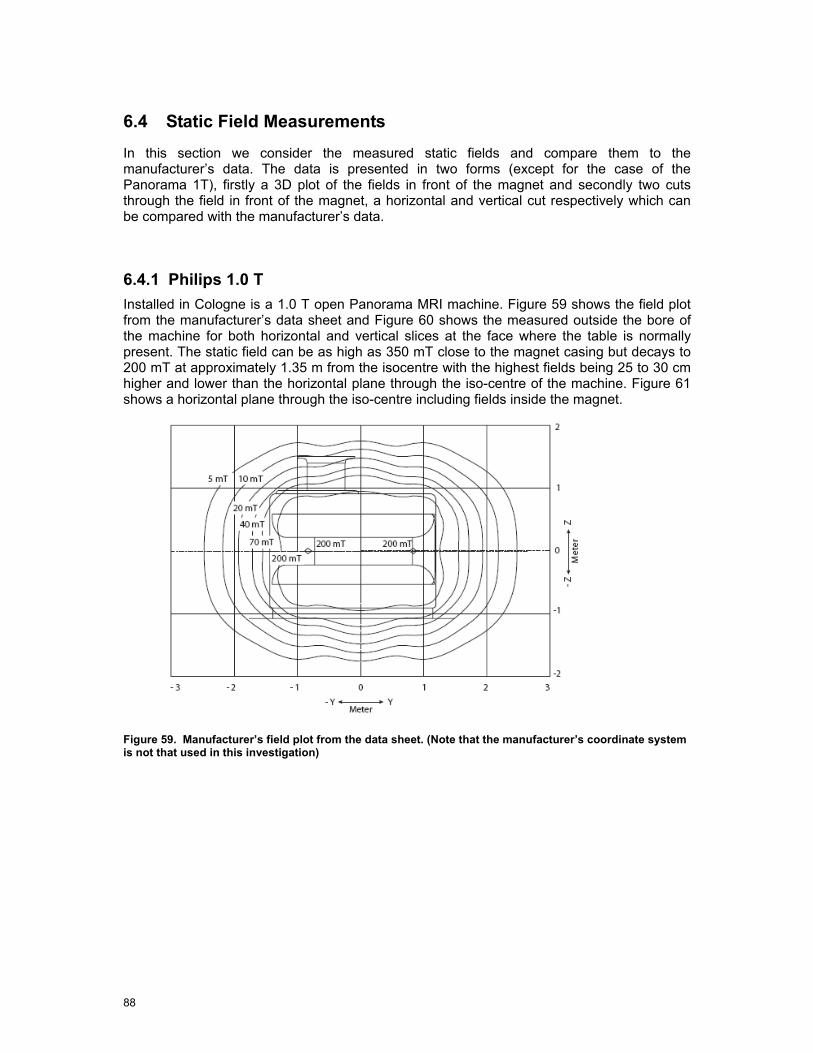
88
6.4 Static Field Measurements
In this section we consider the measured static fields and compare them to the manufacturer’s data. The data is presented in two forms (except for the case of the Panorama 1T), firstly a 3D plot of the fields in front of the magnet and secondly two cuts through the field in front of the magnet, a horizontal and vertical cut respectively which can be compared with the manufacturer’s data.
6.4.1 Philips 1.0 T Installed in Cologne is a 1.0 T open Panorama MRI machine. Figure 59 shows the field plot from the manufacturer’s data sheet and Figure 60 shows the measured outside the bore of the machine for both horizontal and vertical slices at the face where the table is normally present. The static field can be as high as 350 mT close to the magnet casing but decays to 200 mT at approximately 1.35 m from the isocentre with the highest fields being 25 to 30 cm higher and lower than the horizontal plane through the iso-centre of the machine. Figure 61 shows a horizontal plane through the iso-centre including fields inside the magnet.
Figure 59. Manufacturer’s field plot from the data sheet. (Note that the manufacturer’s coordinate system is not that used in this investigation)

89
Horizontal Slice
Vertical Slice
Figure 60. 1.0 T Panorama, static field magnitude, slices outside the bore. Contours in mT.
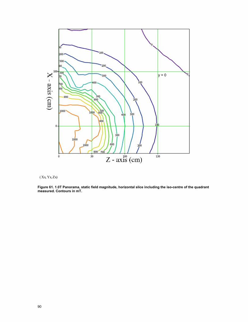
90
Xx Yx, Zx,( )
y = 0
Figure 61. 1.0T Panorama, static field magnitude, horizontal slice including the iso-centre of the quadrant measured. Contours in mT.
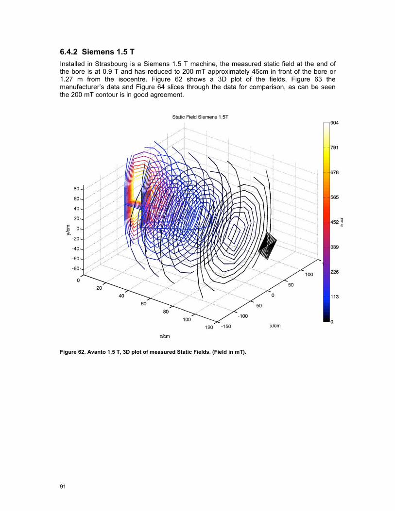
91
6.4.2 Siemens 1.5 T Installed in Strasbourg is a Siemens 1.5 T machine, the measured static field at the end of the bore is at 0.9 T and has reduced to 200 mT approximately 45cm in front of the bore or 1.27 m from the isocentre. Figure 62 shows a 3D plot of the fields, Figure 63 the manufacturer’s data and Figure 64 slices through the data for comparison, as can be seen the 200 mT contour is in good agreement.
Figure 62. Avanto 1.5 T, 3D plot of measured Static Fields. (Field in mT).
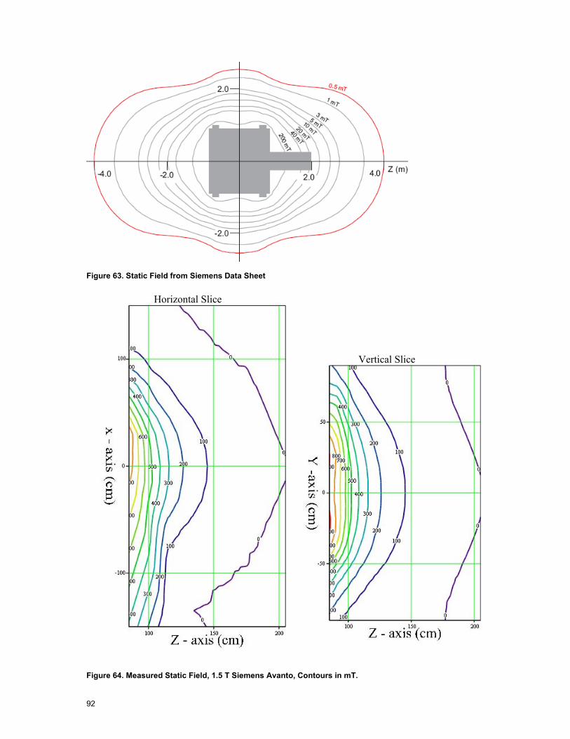
92
Figure 63. Static Field from Siemens Data Sheet
Horizontal Slice
Vertical Slice
Figure 64. Measured Static Field, 1.5 T Siemens Avanto, Contours in mT.

93
6.4.3 Philips 3.0 T Achieva Installed in Leuven is a Philips 3.0 T Achieva machine, the measured static field at the end of the bore is at 1.2 T and has reduced to 200 mT approximately 55 cm in front of the bore or 1.48 m from the isocentre. Figure 65 shows a 3D plot of the fields, Figure 66 the manufacturer’s data and Figure 67 slices through the data for comparison, as can be seen the 200 mT contour is in good agreement.
Figure 65. Philips 3.0 T Achieva, 3D plot of measured Static Fields. (Field in mT).
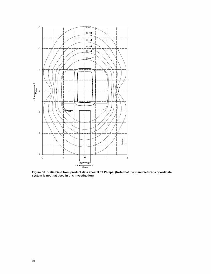
94
Figure 66. Static Field from product data sheet 3.0T Philips. (Note that the manufacturer’s coordinate system is not that used in this investigation)
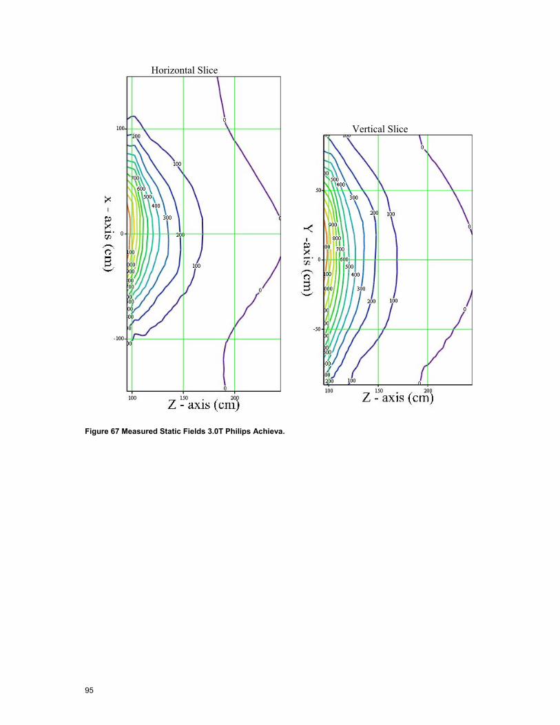
95
Horizontal Slice
Vertical Slice
Figure 67 Measured Static Fields 3.0T Philips Achieva.
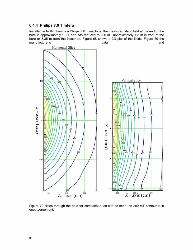
96
6.4.4 Philips 7.0 T Intera Installed in Nottingham is a Philips 7.0 T machine, the measured static field at the end of the bore is approximately 1.9 T and has reduced to 200 mT approximately 1.5 m in front of the bore or 3.35 m from the isocentre. Figure 68 shows a 3D plot of the fields, Figure 69 the manufacturer’s data and
Horizontal Slice
Vertical Slice
Figure 70 slices through the data for comparison, as can be seen the 200 mT contour is in good agreement.

97
Figure 68. 3D plot of static fields for the 7.0 T Philips Intera.
Figure 69. Field plot for 7.0 T with magnetic shielding room. (Note that the coordinate system is not that used in this investigation)
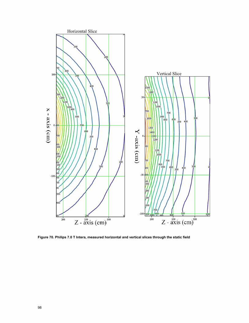
98
Horizontal Slice
Vertical Slice
Figure 70. Philips 7.0 T Intera, measured horizontal and vertical slices through the static field
99
6.5 Static Field Gradients
Movement through a static field can induce currents in the body. The magnitude of the induced currents depends on two factors, namely, spatial gradient of the static field and the velocity of movement. Outside the bore of the machines, it is only the conventional machines that have significant field gradients and the results of the analyses can be seen in the following subsections. The gradient is calculated between adjacent grid points so is effectively half way between the original measurement grid points in all cases.
6.5.1 Siemens 1.5 T Avanto. The static field gradients from the 1.5 T Avanto are shown in terms of the total field gradient in Figure 71 and individual field gradient components (x, y, z) for the two closest measurement planes in Figure 72. The peak gradient is > 3 T/m for this 1.5 T machine. In Figure 71 and Figure 72 the axes are x – horizontal and y – vertical, the variable name for example GX85 denotes G = gradient, X = x static gradient component (could also be Y = y component, Z = z component or Mag = magnitude of the vector sum) and 85 = distance in cm from the iso-centre.

100
GMag85 GMag100
GMag115 GMag130
GMag145 GMag175 Figure 71. Siemens 1.5 T Avanto static field gradient magnitude of x, y and z components, number in the variable name denotes the z distance from the iso-centre. Components have been mirrored for those parts that could not be measured due to the console. Contours are in mT/m. (scale is x 30 cm with the bore-site at the centre of the plot)

101
GX85 GX100
GY85 GY100
GZ85 GZ100
Figure 72. Siemens 1.5 T Avanto x , y and z components of the gradient for the slices closest to the end of the bore. Contours are in mT/m. (scale is x 30 cm with the bore-site at the centre of the plot)
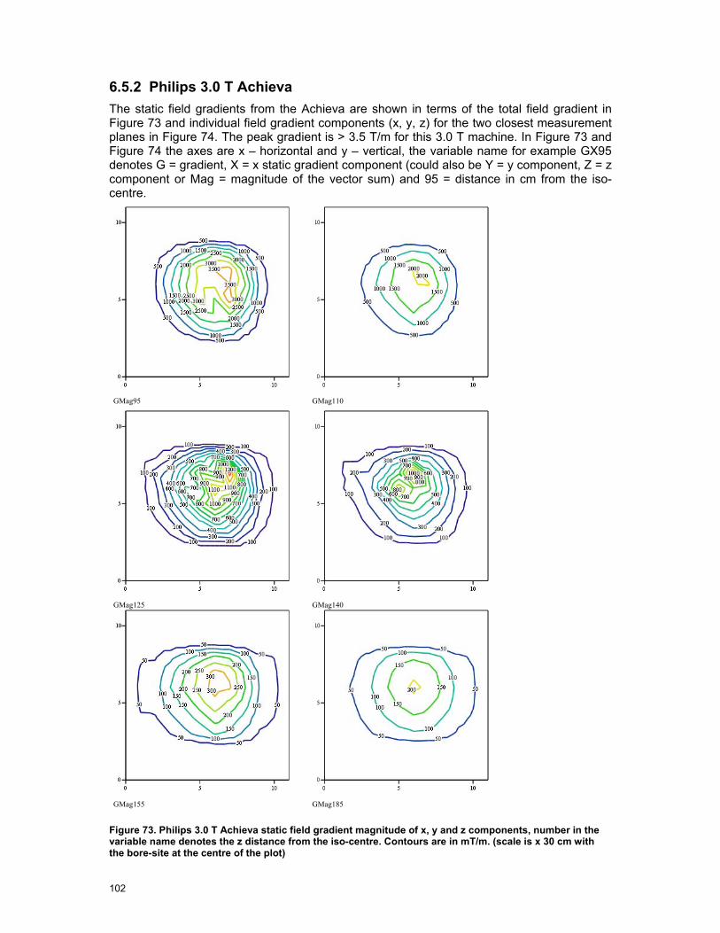
102
6.5.2 Philips 3.0 T Achieva The static field gradients from the Achieva are shown in terms of the total field gradient in Figure 73 and individual field gradient components (x, y, z) for the two closest measurement planes in Figure 74. The peak gradient is > 3.5 T/m for this 3.0 T machine. In Figure 73 and Figure 74 the axes are x – horizontal and y – vertical, the variable name for example GX95 denotes G = gradient, X = x static gradient component (could also be Y = y component, Z = z component or Mag = magnitude of the vector sum) and 95 = distance in cm from the iso-centre.
GMag95 GMag110
GMag125 GMag140
GMag155 GMag185
Figure 73. Philips 3.0 T Achieva static field gradient magnitude of x, y and z components, number in the variable name denotes the z distance from the iso-centre. Contours are in mT/m. (scale is x 30 cm with the bore-site at the centre of the plot)
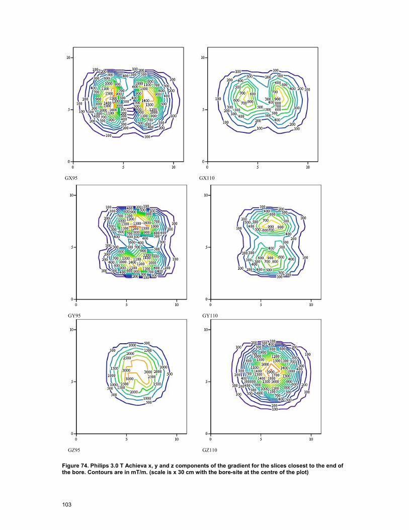
103
GX95 GX110
GY95 GY110
GZ95 GZ110
Figure 74. Philips 3.0 T Achieva x, y and z components of the gradient for the slices closest to the end of the bore. Contours are in mT/m. (scale is x 30 cm with the bore-site at the centre of the plot)
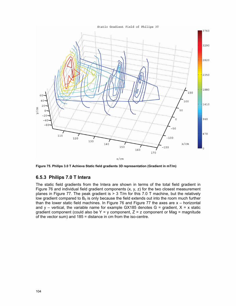
104
Figure 75. Philips 3.0 T Achieva Static field gradients 3D representation (Gradient in mT/m)
6.5.3 Philips 7.0 T Intera The static field gradients from the Intera are shown in terms of the total field gradient in Figure 76 and individual field gradient components (x, y, z) for the two closest measurement planes in Figure 77. The peak gradient is > 3 T/m for this 7.0 T machine, but the relatively low gradient compared to B0 is only because the field extends out into the room much further than the lower static field machines. In Figure 76 and Figure 77 the axes are x – horizontal and y – vertical, the variable name for example GX185 denotes G = gradient, X = x static gradient component (could also be Y = y component, Z = z component or Mag = magnitude of the vector sum) and 185 = distance in cm from the iso-centre.
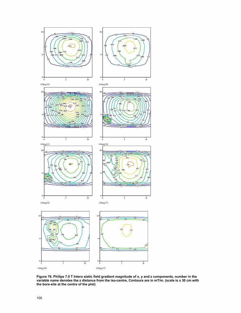
105
GMag185 GMag200
GMag215 GMag230
GMag245 GMag275
GMag305 GMag335
Figure 76. Philips 7.0 T Intera static field gradient magnitude of x, y and z components, number in the variable name denotes the z distance from the iso-centre, Contours are in mT/m. (scale is x 30 cm with the bore-site at the centre of the plot)
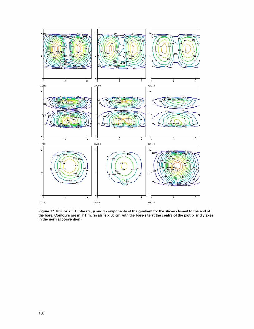
106
GX185 GX200 GX215
GY185 GY200 GY215
GZ185 GZ200 GZ215
Figure 77. Philips 7.0 T Intera x , y and z components of the gradient for the slices closest to the end of the bore. Contours are in mT/m. (scale is x 30 cm with the bore-site at the centre of the plot, x and y axes in the normal convention)
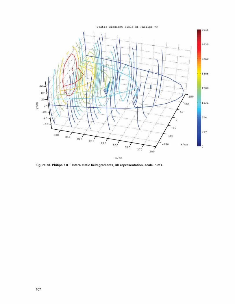
107
Figure 78. Philips 7.0 T Intera static field gradients, 3D representation, scale in mT.

108
6.6 Gradient Field Measurements
The gradient field measurements comprised two elements, firstly measurements of real clinical sequences relevant to the types of interventional MRI performed at the site in question at two locations and secondly the measurement of a test sequence exciting X, Y and Z gradients individually in sequence with known amplitude and rise times for all points on the measurement grid down to 0.1 of the action value. For conventional bore machines when the field probe is placed on bore site at the end of the bore the X, Y and Z components are readily extracted on an individual basis allowing extrapolation to any point on the measurement grid of any clinical sequence. For the open MRI there is such a large variation of the individual components at the reference point at the end of the bore that this process cannot be applied using an identical procedure.
The test sequence for the machines is shown in Figure 79 and the parameters applied in Table 30, the idea was to use a sequence with (or close to) the maximum slew rate and maximum amplitude.
Z
X
Y
5 ms
2 x trrise time tr
0.123 ms
5 ms
50 ms
Amplitude
Figure 79. Gradient Test Sequence
Type of Machine Rise Time Amplitude
1.0 T Panorama 210 µs 16.38 mT/m
1.5 T Siemens Avanto 175 µs 28.0 mT/m
3.0 T Philips Achieva 210 µs 20.1 mT/m
7.0 T Philips Intera 210 µs 20.1 mT/m
Table 30. Gradient test sequence parameters

109
The exposure limit for magnetic gradient fields in Directive 2004/40/EC [13] is based on the ICNIRP 1998 guidelines [10] and specifically the exposure limit values are given in Table 31.
Frequency (Hz)
RMS Current Density (mA/m2) (in central nervous tissues, averaged over 1 cm2 normal to direction of current flow)
< 1 40
1-4 40/f
4 - 103 10
103 - 105 f/100
Table 31. Exposure limits from Directive 2004/40/EC.
The values given in the directive for the exposure limit assume exposure to an electric or magnetic field with a sinusoidal amplitude variation with time. However gradient fields are complex non-sinusoidal pulse sequences and for analysis of their levels of exposure reference was made to the ICNIRP guidance [12] published in 2004. This guidance enables interpretation of the original ICNIRP standard in a way that does not depend on sinusoidal signal characteristics. The extension considers only the rates of change of field and the appropriate weighting of this time derivative of the gradient field, Figure 80.
10 100 1 .103 1 .104 1 .1051 .10 3
0.01
0.1
1
Frequency Hz
Curr
ent D
ensit
y A
/m2
10 100 1 .103 1 .104 1 .1050.1
1
10
100
Frequency Hz
dB/d
t T/
s
10 100 1 .103 1 .104 1 .1050.01
0.1
1
10
Frequency Hz
Wei
ghtin
g Fn
Figure 80. The relationship of the action value limit in dB/dt to the exposure limit.

110
Figure 80 shows, from top to bottom, the action value as stated in Directive 2004/40/EC directive, the conversion of this to a limit in terms of peak rate of change of magnetic field dB/dt and the weighting function to be applied to the dB/dt spectral components respectively.
Using ICNIRP’s simplified body model 064.0
)(2 fJdtdB ⋅
≈ where J(f) is the current density limit.
This gives a limit for the rate of change of field of 0.22 T/s up to a frequency of 1 kHz then increasing as a function of frequency from then on. If dB/dt is measured using a loop sensor then the induced voltage is proportional to dB/dt and applying a low pass filter function can give a direct read out with respect to the limit (high frequencies contribute less). In the original ICNIRP standard the corner frequency is 1 kHz, however in the 2004 guidance a corner frequency of 820Hz is chosen, this effectively increases the limit very slightly above 820Hz. In this work we have used this more flexible and applicable action value of 0.22 T/s throughout. The value of 0.22 T/s would correspond to an equivalent sinusoid amplitude the same as that given for unperturbed rms action values in the Directive 2004/40/EC.
Frequency Range Magnetic Field Strength H A/m
Magnetic Flux Density B µT
8 – 25 Hz 20 x 103 / f (Hz) 25 x 103 / f (Hz)
0.025 – 0.820 kHz 20 / f (kHz) 25 / f (kHz)
0.820 kHz – 65 kHz 24.4 30.7 Table 32. Magnetic field action values from Directive 2004/40/EC [13].
6.6.1 Clinical Sequences Philips Panorama 1.0 T At the position x = 15 cm y = 0 cm and z = 30 cm within the bore of the open MRI the following results for the clinical sequences were recorded. The sequence waveforms of the x, y and z components were captured over 5 seconds and the entire waveform was processed to find the peak exposure values.
6.6.1.1 Planar Echo Sequence, Panorama 1.0 T. The diffusion weighted single shot (DW-SSh) planar echo imaging sequence was recorded for transverse sagittal and coronal planes, the exposure from all planes was similar, Figure 81 and Figure 82 show the sequence in the time domain, the first is the B-field and the second the ICNIRP weighted rate of change of B [3] where the x, y and z components are summed vectorially.
Mag
netic
Fie
ld (T
)
0.1 0.2 0.3 0.4 0.5 0.6 0.7 0.8 0.9 10.004
0.002
0
0.002
0.004
0.006
p
Timeip
Time (s)
Figure 81. DW-SSh sequence in a sagittal plane, amplitude in Tesla, time in seconds. (Red – x axis of ELT-400, Blue – y axis of ELT-400, Green – z axis of ELT-400)
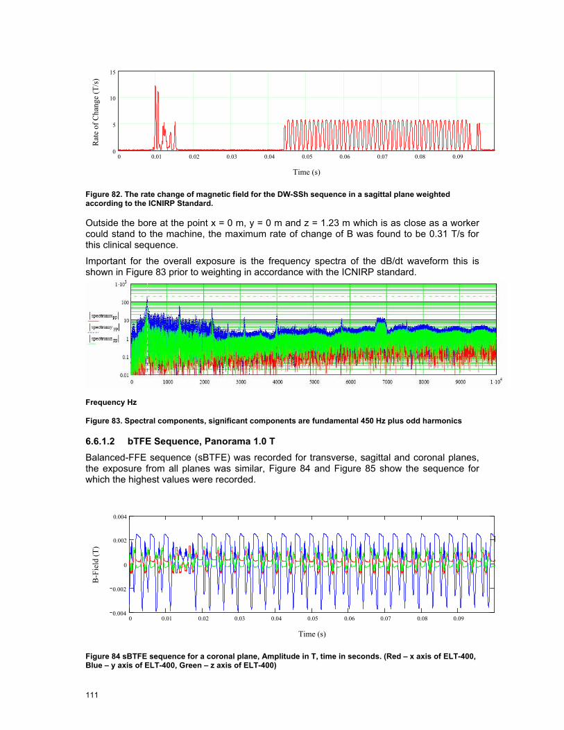
111
0 0.01 0.02 0.03 0.04 0.05 0.06 0.07 0.08 0.090
5
10
15
Time (s)
Rat
e of
Cha
nge
(T/s
)
Figure 82. The rate change of magnetic field for the DW-SSh sequence in a sagittal plane weighted according to the ICNIRP Standard.
Outside the bore at the point x = 0 m, y = 0 m and z = 1.23 m which is as close as a worker could stand to the machine, the maximum rate of change of B was found to be 0.31 T/s for this clinical sequence.
Important for the overall exposure is the frequency spectra of the dB/dt waveform this is shown in Figure 83 prior to weighting in accordance with the ICNIRP standard.
Frequency Hz
Figure 83. Spectral components, significant components are fundamental 450 Hz plus odd harmonics
6.6.1.2 bTFE Sequence, Panorama 1.0 T Balanced-FFE sequence (sBTFE) was recorded for transverse, sagittal and coronal planes, the exposure from all planes was similar, Figure 84 and Figure 85 show the sequence for which the highest values were recorded.
0 0.01 0.02 0.03 0.04 0.05 0.06 0.07 0.08 0.090.004
0.002
0
0.002
0.004
Time (s)
B-F
ield
(T)
Figure 84 sBTFE sequence for a coronal plane, Amplitude in T, time in seconds. (Red – x axis of ELT-400, Blue – y axis of ELT-400, Green – z axis of ELT-400)
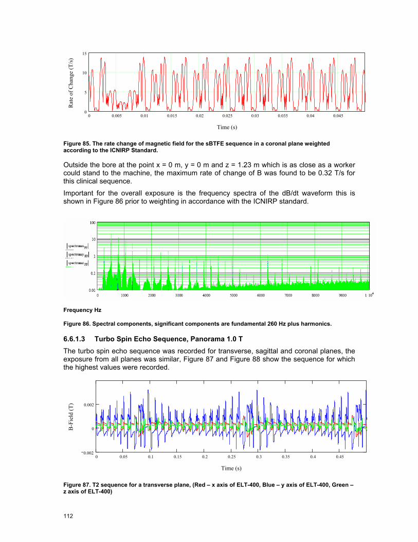
112
0 0.005 0.01 0.015 0.02 0.025 0.03 0.035 0.04 0.0450
5
10
15
Time (s)
Rat
e of
Cha
nge
(T/s
)
Figure 85. The rate change of magnetic field for the sBTFE sequence in a coronal plane weighted according to the ICNIRP Standard.
Outside the bore at the point x = 0 m, y = 0 m and z = 1.23 m which is as close as a worker could stand to the machine, the maximum rate of change of B was found to be 0.32 T/s for this clinical sequence.
Important for the overall exposure is the frequency spectra of the dB/dt waveform this is shown in Figure 86 prior to weighting in accordance with the ICNIRP standard.
Frequency Hz
Figure 86. Spectral components, significant components are fundamental 260 Hz plus harmonics.
6.6.1.3 Turbo Spin Echo Sequence, Panorama 1.0 T The turbo spin echo sequence was recorded for transverse, sagittal and coronal planes, the exposure from all planes was similar, Figure 87 and Figure 88 show the sequence for which the highest values were recorded.
0 0.05 0.1 0.15 0.2 0.25 0.3 0.35 0.4 0.450.002
0
0.002
Time (s)
B-F
ield
(T)
Figure 87. T2 sequence for a transverse plane, (Red – x axis of ELT-400, Blue – y axis of ELT-400, Green – z axis of ELT-400)
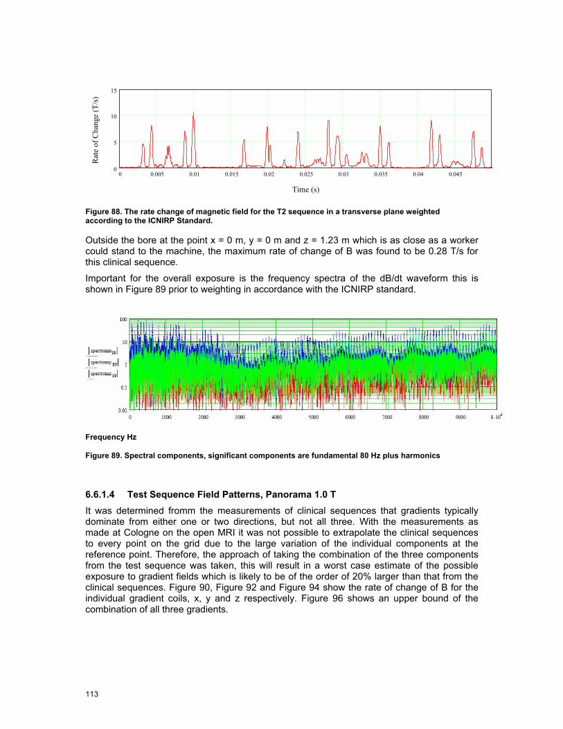
113
0 0.005 0.01 0.015 0.02 0.025 0.03 0.035 0.04 0.0450
5
10
15
Time (s)
Rat
e of
Cha
nge
(T/s
)
Figure 88. The rate change of magnetic field for the T2 sequence in a transverse plane weighted according to the ICNIRP Standard.
Outside the bore at the point x = 0 m, y = 0 m and z = 1.23 m which is as close as a worker could stand to the machine, the maximum rate of change of B was found to be 0.28 T/s for this clinical sequence.
Important for the overall exposure is the frequency spectra of the dB/dt waveform this is shown in Figure 89 prior to weighting in accordance with the ICNIRP standard.
Frequency Hz
Figure 89. Spectral components, significant components are fundamental 80 Hz plus harmonics
6.6.1.4 Test Sequence Field Patterns, Panorama 1.0 T It was determined fromm the measurements of clinical sequences that gradients typically dominate from either one or two directions, but not all three. With the measurements as made at Cologne on the open MRI it was not possible to extrapolate the clinical sequences to every point on the grid due to the large variation of the individual components at the reference point. Therefore, the approach of taking the combination of the three components from the test sequence was taken, this will result in a worst case estimate of the possible exposure to gradient fields which is likely to be of the order of 20% larger than that from the clinical sequences. Figure 90, Figure 92 and Figure 94 show the rate of change of B for the individual gradient coils, x, y and z respectively. Figure 96 shows an upper bound of the combination of all three gradients.
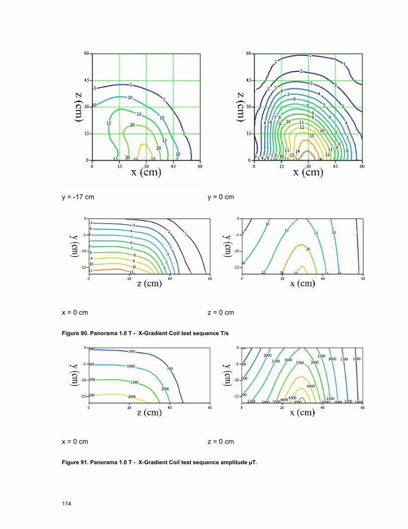
114
y = -17 cm y = 0 cm
x = 0 cm z = 0 cm
Figure 90. Panorama 1.0 T - X-Gradient Coil test sequence T/s
x = 0 cm z = 0 cm
Figure 91. Panorama 1.0 T - X-Gradient Coil test sequence amplitude µT.

115
y = -17 cm y = 0 cm
x = 0 cm z = 0 cm Figure 92. Panorama 1.0 T - Y gradient coil test sequence T/s
x = 0 cm z = 0 cm Figure 93. Panorama 1.0 T - Y gradient coil test sequence amplitude µT
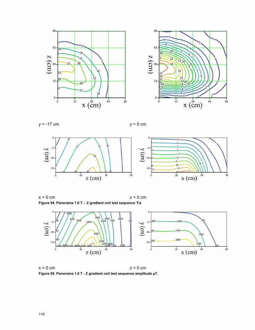
116
y = -17 cm y = 0 cm
x = 0 cm z = 0 cm Figure 94. Panorama 1.0 T - Z gradient coil test sequence T/s
x = 0 cm z = 0 cm Figure 95. Panorama 1.0 T - Z gradient coil test sequence amplitude µT.

117
y = -17 cm y = 0 cm
x = 0 cm z = 0 cm
Figure 96. Panorama 1.0 T - Gradients in the bore assuming excitation of X, Y and Z gradient coils with equal amplitude and vector addition of the components. Contours are labeled in T/s

118
6.6.2 Gradient Test Sequence for Siemens 1.5 T Avanto For the Avanto the test sequence applied was as detailed in Table 30, for this sequence the field distribution inside and outside the bore of the machine can be mapped. Cross correlation techniques using a standard copy of the waveform are used to obtain best accuracy for the pulse amplitude extraction.
y = 0 cm x = 0 cm Figure 97. 1.5 T Avanto - Y gradient coil amplitudes in the bore µT
y = 0 cm x = 0 cm Figure 98. 1.5 T Avanto - X gradient coil amplitudes in the bore µT
y = 0 cm x = 0 cm Figure 99. 1.5 T Avanto - Z gradient coil amplitudes in the bore µT

119
6.6.3 Clinical Sequence Gradient Fields Siemens 1.5T
6.6.3.1 EPI Sequence, 1.5 T Avanto At the reference position, on the axis of the bore 95 cm in front of the isocentre the maximum exposure from this sequence is 1.98 T/s which is 9 times the action value.
The sequence waveforms of the x, y and z components were captured over 5 seconds and the entire waveform was processed, Figure 100, Figure 101 and Figure 102 show parts of the waveforms for illustrative purposes.
M
agne
tic F
ield
(T)
0.04 0.05 0.06 0.07 0.08 0.09 0.1 0.11 0.12 0.13 0.14 0.15 0.16 0.170.001
5 .10 4
0
5 .10 4
0.001
0.0015
i
Time (s)
Figure 100. EPI time domain B-field (T) (Red – x axis of ELT-400, Blue – y axis of ELT-400, Green – z axis of ELT-400)
dB
/dt (
T/s)
0.04 0.05 0.06 0.07 0.08 0.09 0.1 0.11 0.12 0.13 0.14 0.15 0.16 0.174
2
0
2
4
6
p
p
p
Time (s)
Figure 101. Rate of change of B-Field (T/s) (Red – x axis of ELT-400, Blue – y axis of ELT-400, Green – z axis of ELT-400)
0 0.002 0.004 0.006 0.008 0.01 0.012 0.014 0.016 0.0182
0
2
Time (s)
X, Y
& Z
fiel
ds (T
/s)
( )
Figure 102. The part of the EPI sequence that has the highest overall rate of change of B-field (at the reference position) is shown at the centre of the graph with 0.01 seconds either side (T/s). The sequence

120
has been weighted in the frequency domain in accordance to the ICNIRP standard. (Red – x axis of ELT-400, Blue – y axis of ELT-400, Green – z axis of ELT-400)
0 0.02 0.04 0.06 0.08 0.1 0.12 0.14 0.16 0.18 0.2 0.22 0.240
0.5
1
1.5
2
Time (s)
Rat
e of
Cha
nge
of B
(T/s
)
Figure 103. Total gradient B-field.
Figure 103 shows the vector sum of the three gradient components and hence the total gradient field exposure at the reference point.
Important for the overall exposure is the frequency spectra of the dB/dt waveform this is shown in Figure 104 prior to weighting in accordance with the ICNIRP standard.
Frequency Hz
Figure 104. Spectral components, significant components are fundamental 670 Hz plus harmonics

121
z =
85 c
m
z =
100
cm
z =
115
cm
z =
130
cm
z =
145
cm
z =
175
cm
y↑
X85 Y85, Z85,( ) X100 Y100, Z100,( )
X115 Y115, Z115,( ) X130 Y130, Z130,( )
X145 Y145, Z145,( ) X175 Y175, Z175,( )
x→
Figure 105. 1.5 T Avanto. Slices through the space in front of the machine (numbers in the variables note the distance from the isocentre in cm). Each slice is individually scaled, contours labelled in T/s.

122
y = 0 cm x = 0 cm
Figure 106. 1.5 T Avanto. In the bore gradient fields for the EPI sequence, contours in T/s.

123
6.6.3.2 TrueFISP Sequence, 1.5 T Avanto At the reference position, on the bore axis 95 cm from the isocentre the maximum exposure from this sequence is 1.99 T/s which is 9 times the action value.
The sequence waveforms of the x, y and z components were captured over 5 seconds and the entire waveform was processed, Figure 107, Figure 108 and Figure 109 show parts of the waveforms for illustrative purposes.
M
agne
tic F
ield
(T)
0.3 0.305 0.31 0.315 0.32 0.325 0.33 0.335 0.34 0.3455 .10 4
0
5 .10 4
p
p
Time (s)
Figure 107. TrueFISP time domain B-field (T) (Red – x axis of ELT-400, Blue – y axis of ELT-400, Green – z axis of ELT-400)
dB
/dt (
T/s)
0.3 0.305 0.31 0.315 0.32 0.325 0.33 0.335 0.34 0.3454
2
0
2
4
p
Time (s)
Figure 108. Rate of change of B-Field (T/s) (Red – x axis of ELT-400, Blue – y axis of ELT-400, Green – z axis of ELT-400)
0 0.002 0.004 0.006 0.008 0.01 0.012 0.014 0.016 0.0182
0
2
Time (s)
X, Y
& Z
fiel
ds (T
/s)
Figure 109. The part of the TrueFISP sequence that has the highest overall rate of change of B-field (at the reference position) is shown at the centre of the graph with 500 samples either side (T/s). The sequence has been weighted in the frequency domain in accordance to the ICNIRP standard. (Red – x axis of ELT-400, Blue – y axis of ELT-400, Green – z axis of ELT-400)

124
0 0.005 0.01 0.015 0.02 0.025 0.03 0.035 0.04 0.0450
0.5
1
1.5
2
Time (s)
Rat
e of
Cha
nge
of B
(T/s
)
Figure 110. Vector sum of the gradient fields
Important for the overall exposure is the frequency spectra of the dB/dt waveform this is shown in Figure 104 prior to weighting in accordance with the ICNIRP standard.
Frequency Hz
Figure 111. Spectral components, significant components are fundamental 400 Hz plus harmonics
The following plots show the gradient fields outside the bore (Figure 112) and inside the bore (Figure 113) in T/s for the 1.5 T Avanto.

125
z
= 85
cm
z =
100
cm
z =
115
cm
z =
130
cm
z =
145
cm
z =
175
cm
y↑
X85 Y85, Z85,( ) X100 Y100, Z100,( )
X115 Y115, Z115,( ) X130 Y130, Z130,( )
X145 Y145, Z145,( ) X175 Y175, Z175,( ) x→
Figure 112. 1.5 T Avanto. Slices through the space in front of the machine (numbers in the variables note the distance from the iso centre in cm). Each slice is individually scaled, contours labelled in T/s.
Figure 113. 1.5 T Avanto. In the bore gradient fields for the True Fisp sequence, contours in T/s.
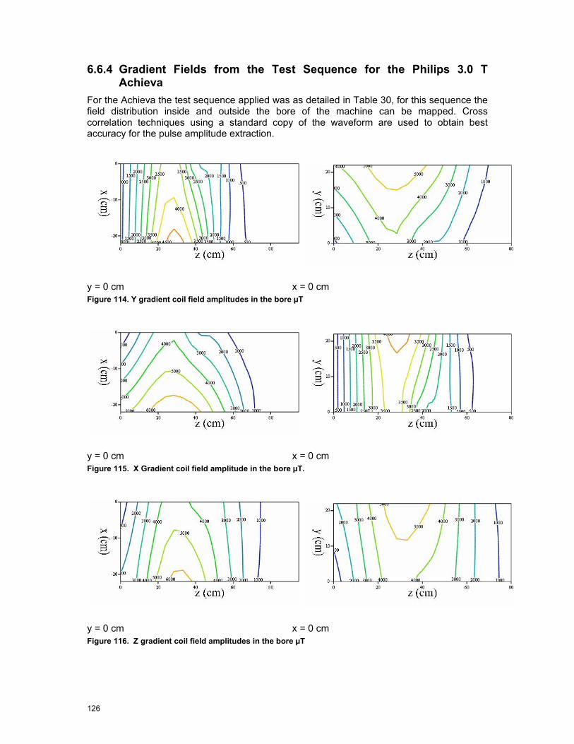
126
6.6.4 Gradient Fields from the Test Sequence for the Philips 3.0 T Achieva
For the Achieva the test sequence applied was as detailed in Table 30, for this sequence the field distribution inside and outside the bore of the machine can be mapped. Cross correlation techniques using a standard copy of the waveform are used to obtain best accuracy for the pulse amplitude extraction.
y = 0 cm x = 0 cm Figure 114. Y gradient coil field amplitudes in the bore µT
y = 0 cm x = 0 cm Figure 115. X Gradient coil field amplitude in the bore µT.
y = 0 cm x = 0 cm Figure 116. Z gradient coil field amplitudes in the bore µT

127
6.6.5 Clinical Sequence Gradient Fields Philips 3.0 T Achieva
6.6.5.1 Turbo Spin Echo Sequence, 3.0 T Achieva At the reference position, on bore sight 95cm in front of the isocentre the maximum exposure from this sequence is 0.313 T/s which is 1.4 times the action value.
The sequence waveforms of the x, y and z components were captured over 5 seconds and the entire waveform was processed, Figure 117, Figure 118 and Figure 119 show parts of the waveforms for illustrative purposes.
M
agne
tic F
ield
(T)
0.16 0.18 0.2 0.22 0.24 0.26 0.28 0.3 0.32 0.34 0.36 0.382 .10 4
1 .10 4
0
1 .10 4
2 .10 4
p
p
p
Time (s)
Figure 117. Turbo spin echo B-field as a function of time (T) (Red – x axis of ELT-400, Blue – y axis of ELT-400, Green – z axis of ELT-400)
dB/d
t (T/
s)
0.16 0.18 0.2 0.22 0.24 0.26 0.28 0.3 0.32 0.34 0.36 0.380.4
0.2
0
0.2
0.4
p
p
p
Time (s)
Figure 118. Turbo spin echo sequence rates of change of B-field (T/s) (Red – x axis of ELT-400, Blue – y axis of ELT-400, Green – z axis of ELT-400)
dB/d
t (T/
s)
0 100 200 300 400 500 600 700 800 900 10000.4
0.2
0
0.2
0.4
Time (samples)
Figure 119. The part of the Turbo spin echo sequence that has the highest overall rate of change of B-field (at the reference position) is shown at the centre of the graph with 500 samples either side (T/s). The

128
sequence has been weighted in the frequency domain in accordance to the ICNIRP standard. (Red – x gradient, Blue – y gradient, Green – z Gradient)
0 0.02 0.04 0.06 0.08 0.1 0.12 0.14 0.16 0.180
0.1
0.2
0.3
0.4
Time (s)
Rat
e of
Cha
nge
of B
(T/s
)
Figure 120. Vector sum of x, y and z components showing the overall gradient
The highest exposure for all other positions might be a different part of the waveform due to the variation in the relative contributions from the x, y and z gradients and is determined individually for each measurement position.
Important for the overall exposure is the frequency spectra of the dB/dt waveform this is shown in Figure 121 prior to weighting in accordance with the ICNIRP standard.
Frequency Hz
Figure 121. Spectral components, significant components are fundamental 100 Hz plus harmonics
The clinical sequence is weighted according to the measured test sequence distribution and the resultant field plots shown in Figure 122 and Figure 123.

129
z
= 95
cm
z =
110
cm
z =
125
cm
z =
140
cm
z =
155
cm
z =
185
cm
y↑
X95 Y95, Z95,( ) X110 Y110, Z110,( )
X125 Y125, Z125,( ) X140 Y140, Z140,( )
X155 Y155, Z155,( ) X185 Y185, Z185,( )
x→
Figure 122. 3.0 T Achieva. T2 sequence slices through the space in front of the machine (numbers in the variables note the distance from the iso centre in cm). Contour in T/s.
Figure 123. 3.0 T Achieva. Turbo spin echo sequence gradient fields inside the bore, contours in T/s.

130
6.6.5.2 Balanced FFE Sequence, 3.0 T Achieva. At the reference position, on the bore axis 95 cm in front of the isocentre the maximum exposure from this sequence is 0.812 T/s which is 3.7 times the action value.
The sequence waveforms of the x, y and z components were captured over 5 seconds and the entire waveform was processed, Figure 124, Figure 125 and Figure 126 show parts of the waveforms for illustrative purposes.
Mag
netic
fiel
d (T
)
0 0.02 0.04 0.06 0.08 0.1 0.12 0.14 0.16 0.182 .10 4
1 .10 4
0
1 .10 4
2 .10 4
p
Time (s)
Figure 124. Balanced FFE time domain B-field (T) (Red – x axis of ELT-400, Blue – y axis of ELT-400, Green – z axis of ELT-400)
dB/d
t (T/
s)
0 0.001 0.002 0.003 0.004 0.005 0.006 0.007 0.008 0.0091
0.5
0
0.5
1
p
p
Time (s)
Figure 125. Balanced FFE Rate of change of B-Field (T/s) (Red – x axis of ELT-400, Blue – y axis of ELT-400, Green – z axis of ELT-400)
dB/d
t (T/
s)
0 100 200 300 400 500 600 700 800 900 10001
0.5
0
0.5
1
Time (samples)
Figure 126. The part of the balanced FFE sequence that has the highest overall rate of change of B-field (at the reference position) is shown at the centre of the graph with 500 samples either side (T/s). The sequence has been weighted in the frequency domain in accordance to the ICNIRP standard.

131
0 0.01 0.02 0.03 0.04 0.05 0.06 0.07 0.08 0.090
0.5
1
Time (s)
Rat
e of
Cha
nge
of B
(T/s
)
Figure 127. Vector sum of x, y and z components of the gradient field
The highest exposure for all other positions might be a different part of the waveform due to the variation in the relative contributions from the x, y and z gradients and is determined individually for each measurement position.
Important for the overall exposure is the frequency spectra of the dB/dt waveform this is shown in Figure 128 prior to weighting in accordance with the ICNIRP standard.
Frequency Hz
Figure 128. Spectral components, significant components are fundamental 240 Hz plus harmonics
The clinical sequence is weighted according to the measured test sequence distribution and the resultant field plots shown in Figure 129 and Figure 130.
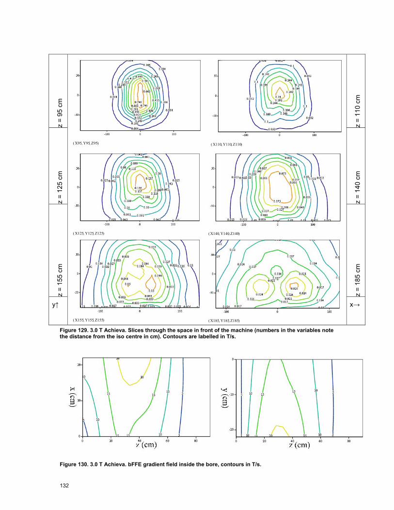
132
z
= 95
cm
z =
110
cm
z =
125
cm
z =
140
cm
z =
155
cm
z =
185
cm
y↑
X95 Y95, Z95,( ) X110 Y110, Z110,( )
X125 Y125, Z125,( ) X140 Y140, Z140,( )
X155 Y155, Z155,( ) X185 Y185, Z185,( )
x→
Figure 129. 3.0 T Achieva. Slices through the space in front of the machine (numbers in the variables note the distance from the iso centre in cm). Contours are labelled in T/s.
Figure 130. 3.0 T Achieva. bFFE gradient field inside the bore, contours in T/s.
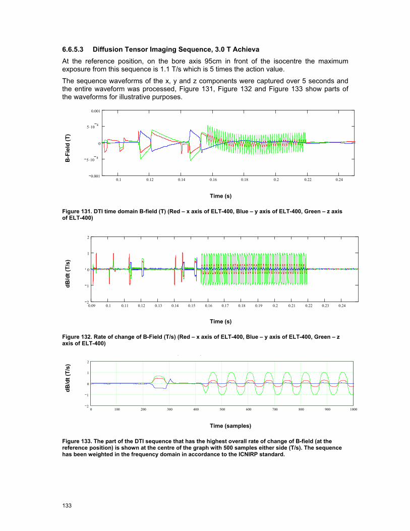
133
6.6.5.3 Diffusion Tensor Imaging Sequence, 3.0 T Achieva At the reference position, on the bore axis 95cm in front of the isocentre the maximum exposure from this sequence is 1.1 T/s which is 5 times the action value.
The sequence waveforms of the x, y and z components were captured over 5 seconds and the entire waveform was processed, Figure 131, Figure 132 and Figure 133 show parts of the waveforms for illustrative purposes.
B-F
ield
(T)
0.1 0.12 0.14 0.16 0.18 0.2 0.22 0.240.001
5 .10 4
0
5 .10 4
0.001
p
Time (s)
Figure 131. DTI time domain B-field (T) (Red – x axis of ELT-400, Blue – y axis of ELT-400, Green – z axis of ELT-400)
dB/d
t (T/
s)
0.09 0.1 0.11 0.12 0.13 0.14 0.15 0.16 0.17 0.18 0.19 0.2 0.21 0.22 0.23 0.242
1
0
1
2
p
p
Time (s)
Figure 132. Rate of change of B-Field (T/s) (Red – x axis of ELT-400, Blue – y axis of ELT-400, Green – z axis of ELT-400)
dB/d
t (T/
s)
0 100 200 300 400 500 600 700 800 900 10002
1
0
1
2
Time (samples)
Figure 133. The part of the DTI sequence that has the highest overall rate of change of B-field (at the reference position) is shown at the centre of the graph with 500 samples either side (T/s). The sequence has been weighted in the frequency domain in accordance to the ICNIRP standard.
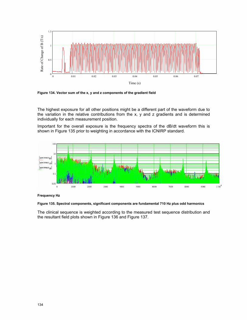
134
0 0.01 0.02 0.03 0.04 0.05 0.06 0.070
0.5
1
1.5
Time (s)
Rat
e of
Cha
nge
of B
(T/s
)
Figure 134. Vector sum of the x, y and z components of the gradient field
The highest exposure for all other positions might be a different part of the waveform due to the variation in the relative contributions from the x, y and z gradients and is determined individually for each measurement position.
Important for the overall exposure is the frequency spectra of the dB/dt waveform this is shown in Figure 135 prior to weighting in accordance with the ICNIRP standard.
Frequency Hz
Figure 135. Spectral components, significant components are fundamental 710 Hz plus odd harmonics
The clinical sequence is weighted according to the measured test sequence distribution and the resultant field plots shown in Figure 136 and Figure 137.

135
z =
95 c
m
z =
110
cm
z =
125
cm
z =
140
cm
z =
155
cm
z =
185
cm
y↑
X95 Y95, Z95,( ) X110 Y110, Z110,( )
X125 Y125, Z125,( ) X140 Y140, Z140,( )
X155 Y155, Z155,( ) X185 Y185, Z185,( )
x→
Figure 136. 3.0 T Achieva. Slices through the space in front of the machine (numbers in the variables note the distance from the iso centre in cm). Each slice is individually scaled.
Figure 137. 3.0 T Achieva. DTI gradient field inside the bore, contours in T/s.

136
6.6.5.4 EPI Sequence, 3.0 T Achieva At the reference position, on the bore axis 95cm in front of the isocentre the maximum exposure from this sequence is 1.69 T/s which is 7.7 times the action value.
The sequence waveforms of the x, y and z components were captured over 5 seconds and the entire waveform was processed, Figure 138, Figure 139 and Figure 140 show parts of the waveforms for illustrative purposes.
dB/d
t (T/
s)
0 0.001 0.002 0.003 0.004 0.005 0.006 0.007 0.008 0.0094 .10 4
2 .10 4
0
2 .10 4
4 .10 4
p
Time (s)
Figure 138. EPI time domain B-field (T) (Red – x axis of ELT-400, Blue – y axis of ELT-400, Green – z axis of ELT-400)
dB/d
t (T/
s)
0 0.001 0.002 0.003 0.004 0.005 0.006 0.007 0.008 0.0092
1
0
1
2
p
p
p
Time (s)
Figure 139. Rate of change of B-Field (T/s) (Red – x axis of ELT-400, Blue – y axis of ELT-400, Green – z axis of ELT-400)
dB/d
t (T/
s)
0 100 200 300 400 500 600 700 800 900 10002
0
2
Time (samples)
Figure 140. The part of the EPI sequence that has the highest overall rate of change of B-field (at the reference position) is shown at the centre of the graph with 500 samples either side (T/s). The sequence has been weighted in the frequency domain in accordance to the ICNIRP standard.

137
0.06 0.065 0.07 0.075 0.08 0.085 0.09 0.095 0.1 0.105 0.11 0.115 0.12 0.1250
0.5
1
1.5
2
Time (s)
Rat
e of
Cha
nge
of B
(T/s
)
Figure 141. Vector sum of the x, y and z components of the gradient field
The highest exposure for all other positions might be a different part of the waveform due to the variation in the relative contributions from the x, y and z gradients and is determined individually for each measurement position.
Important for the overall exposure is the frequency spectra of the dB/dt waveform this is shown in Figure 142 prior to weighting in accordance with the ICNIRP standard.
Frequency Hz
Figure 142. Spectral components, significant components are fundamental 1 kHz plus odd harmonics
The clinical sequence is weighted according to the measured test sequence distribution and the resultant field plots shown in Figure 143 and Figure 144.

138
z =
95 c
m
z =
110
cm
z =
125
cm
z =
140
cm
z =
155
cm
z =
185
cm
y↑
X95 Y95, Z95,( ) X110 Y110, Z110,( )
X125 Y125, Z125,( ) X140 Y140, Z140,( )
X155 Y155, Z155,( ) X185 Y185, Z185,( )
x→
Figure 143. 3.0 T Achieva. Slices through the space in front of the machine (numbers in the variables note the distance from the iso centre in cm). Contours are in T/s, x and y axes are x and y in cm.
Figure 144. 3.0 T Achieva. Gradient fields inside the bore of the scanner (T/s)
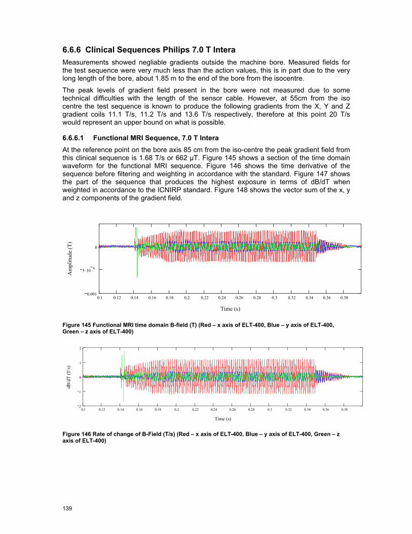
139
6.6.6 Clinical Sequences Philips 7.0 T Intera Measurements showed negliable gradients outside the machine bore. Measured fields for the test sequence were very much less than the action values, this is in part due to the very long length of the bore, about 1.85 m to the end of the bore from the isocentre.
The peak levels of gradient field present in the bore were not measured due to some technical difficulties with the length of the sensor cable. However, at 55cm from the iso centre the test sequence is known to produce the following gradients from the X, Y and Z gradient coils 11.1 T/s, 11.2 T/s and 13.6 T/s respectively, therefore at this point 20 T/s would represent an upper bound on what is possible.
6.6.6.1 Functional MRI Sequence, 7.0 T Intera At the reference point on the bore axis 85 cm from the iso-centre the peak gradient field from this clinical sequence is 1.68 T/s or 662 µT. Figure 145 shows a section of the time domain waveform for the functional MRI sequence. Figure 146 shows the time derivative of the sequence before filtering and weighting in accordance with the standard. Figure 147 shows the part of the sequence that produces the highest exposure in terms of dB/dT when weighted in accordance to the ICNIRP standard. Figure 148 shows the vector sum of the x, y and z components of the gradient field.
0.1 0.12 0.14 0.16 0.18 0.2 0.22 0.24 0.26 0.28 0.3 0.32 0.34 0.36 0.380.001
5 .10 4
0
Time (s)
Am
plitu
de (T
)
Figure 145 Functional MRI time domain B-field (T) (Red – x axis of ELT-400, Blue – y axis of ELT-400, Green – z axis of ELT-400)
0.1 0.12 0.14 0.16 0.18 0.2 0.22 0.24 0.26 0.28 0.3 0.32 0.34 0.36 0.382
1
0
1
2
Time (s)
dB/d
T (T
/s)
Figure 146 Rate of change of B-Field (T/s) (Red – x axis of ELT-400, Blue – y axis of ELT-400, Green – z axis of ELT-400)

140
0 100 200 300 400 500 600 700 800 900 10002
0
2
Time (samples)
dB/d
T (T
/s)
Figure 147 The part of the FMRI sequence that has the highest overall rate of change of B-field (at the reference position) is shown at the centre of the graph with 500 samples either side (T/s). The sequence has been weighted in the frequency domain in accordance to the ICNIRP standard.
0 0.01 0.02 0.03 0.04 0.05 0.06 0.07 0.08 0.090
0.5
1
1.5
2
Time (s)
Rat
e of
Cha
nge
of B
(T/s
)
Figure 148 Vector sum of the x, y and z components of the gradient field (filtered in accordance with the ICNIRP standard)
Important for the overall exposure is the frequency spectra of the dB/dt waveform this is shown in Figure 149 prior to weighting in accordance with the ICNIRP standard.
Figure 149. Spectral components, significant components are fundamental 500 Hz plus harmonics
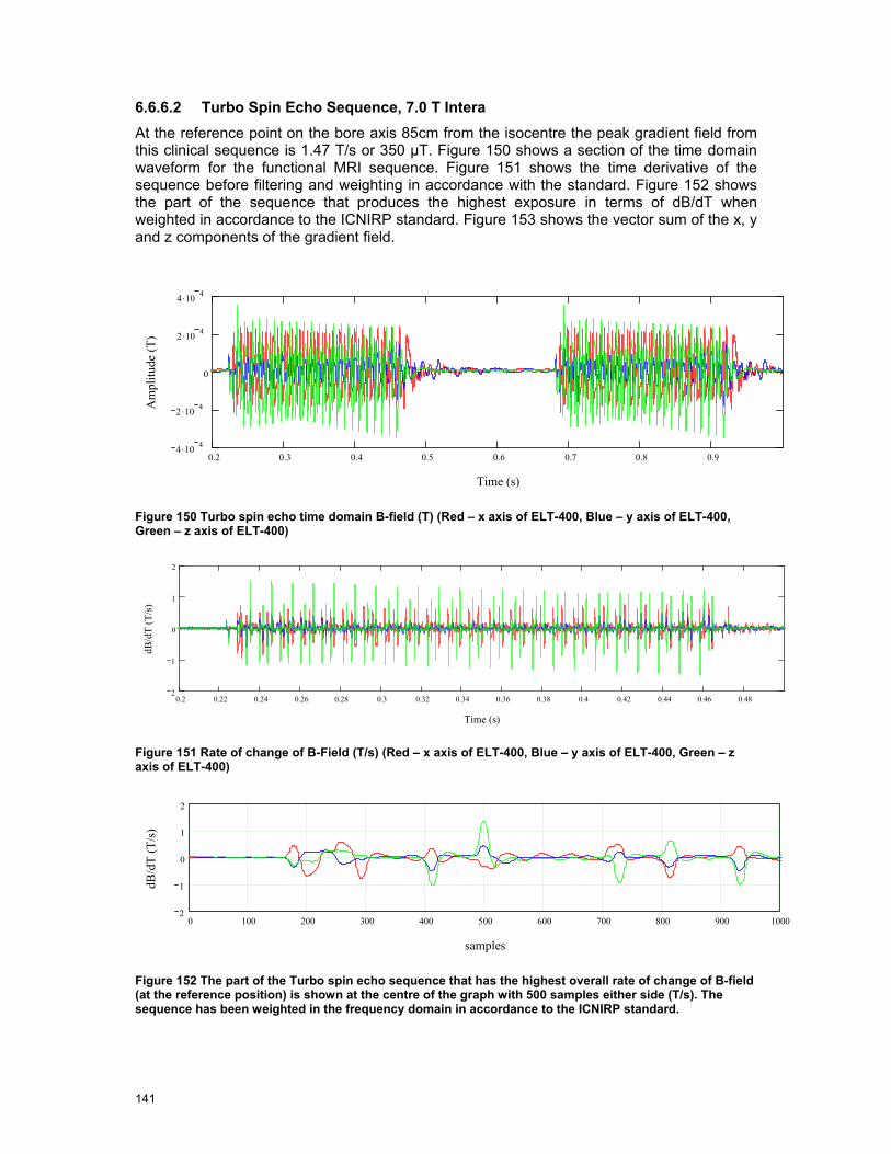
141
6.6.6.2 Turbo Spin Echo Sequence, 7.0 T Intera At the reference point on the bore axis 85cm from the isocentre the peak gradient field from this clinical sequence is 1.47 T/s or 350 µT. Figure 150 shows a section of the time domain waveform for the functional MRI sequence. Figure 151 shows the time derivative of the sequence before filtering and weighting in accordance with the standard. Figure 152 shows the part of the sequence that produces the highest exposure in terms of dB/dT when weighted in accordance to the ICNIRP standard. Figure 153 shows the vector sum of the x, y and z components of the gradient field.
0.2 0.3 0.4 0.5 0.6 0.7 0.8 0.94 .10 4
2 .10 4
0
2 .10 4
4 .10 4
Time (s)
Am
plitu
de (T
)
Figure 150 Turbo spin echo time domain B-field (T) (Red – x axis of ELT-400, Blue – y axis of ELT-400, Green – z axis of ELT-400)
0.2 0.22 0.24 0.26 0.28 0.3 0.32 0.34 0.36 0.38 0.4 0.42 0.44 0.46 0.482
1
0
1
2
Time (s)
dB/d
T (T
/s)
Figure 151 Rate of change of B-Field (T/s) (Red – x axis of ELT-400, Blue – y axis of ELT-400, Green – z axis of ELT-400)
0 100 200 300 400 500 600 700 800 900 10002
1
0
1
2
samples
dB/d
T (T
/s)
Figure 152 The part of the Turbo spin echo sequence that has the highest overall rate of change of B-field (at the reference position) is shown at the centre of the graph with 500 samples either side (T/s). The sequence has been weighted in the frequency domain in accordance to the ICNIRP standard.

142
0 0.01 0.02 0.03 0.04 0.05 0.06 0.07 0.08 0.090
0.5
1
1.5
Time (s)
Rat
e of
Cha
nge
of B
(T/s
)
Figure 153 Vector sum of the x, y and z components of the gradient field (filtered in accordance with the ICNIRP standard)
Important for the overall exposure is the frequency spectra of the dB/dt waveform this is shown in Figure 154 prior to weighting in accordance with the ICNIRP standard.
Figure 154. Spectral components, significant components are fundamental 96 Hz plus harmonics
6.6.6.3 Perfusion Sequence, 7.0 T Intera At the reference point on the bore axis 85cm from the isocentre the peak gradient field from this clinical sequence is 1.78 T/s or 510 µT. Figure 155 shows a section of the time domain waveform for the functional MRI sequence. Figure 156 shows the time derivative of the sequence before filtering and weighting in accordance with the standard. Figure 157 shows the part of the sequence that produces the highest exposure in terms of dB/dT when weighted in accordance to the ICNIRP standard. Figure 158 shows the vector sum of the x, y and z components of the gradient field.

143
0 0.02 0.04 0.06 0.08 0.1 0.12 0.14 0.16 0.18 0.2 0.22 0.24 0.26 0.285 .10 4
0
5 .10 4
Time (s)
Am
plitu
de (T
)
Figure 155 Perfusion time domain B-field (T) (Red – x axis of ELT-400, Blue – y axis of ELT-400, Green – z axis of ELT-400)
0 0.01 0.02 0.03 0.04 0.05 0.06 0.07 0.08 0.09 0.1 0.11 0.12 0.13 0.142
1
0
1
2
Time (s)
dB/d
T (T
/s)
Figure 156 Rate of change of B-Field (T/s) (Red – x axis of ELT-400, Blue – y axis of ELT-400, Green – z axis of ELT-400)
0 100 200 300 400 500 600 700 800 900 10002
0
2
Samples
dB/d
T (T
/s)
Figure 157 The part of the perfusion sequence that has the highest overall rate of change of B-field (at the reference position) is shown at the centre of the graph with 500 samples either side (T/s). The sequence has been weighted in the frequency domain in accordance to the ICNIRP standard.
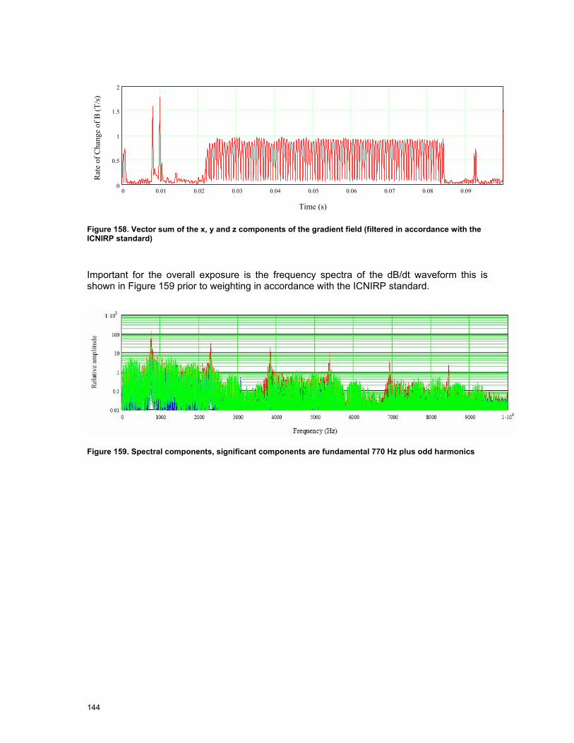
144
0 0.01 0.02 0.03 0.04 0.05 0.06 0.07 0.08 0.090
0.5
1
1.5
2
Time (s)
Rat
e of
Cha
nge
of B
(T/s
)
Figure 158. Vector sum of the x, y and z components of the gradient field (filtered in accordance with the ICNIRP standard)
Important for the overall exposure is the frequency spectra of the dB/dt waveform this is shown in Figure 159 prior to weighting in accordance with the ICNIRP standard.
Figure 159. Spectral components, significant components are fundamental 770 Hz plus odd harmonics
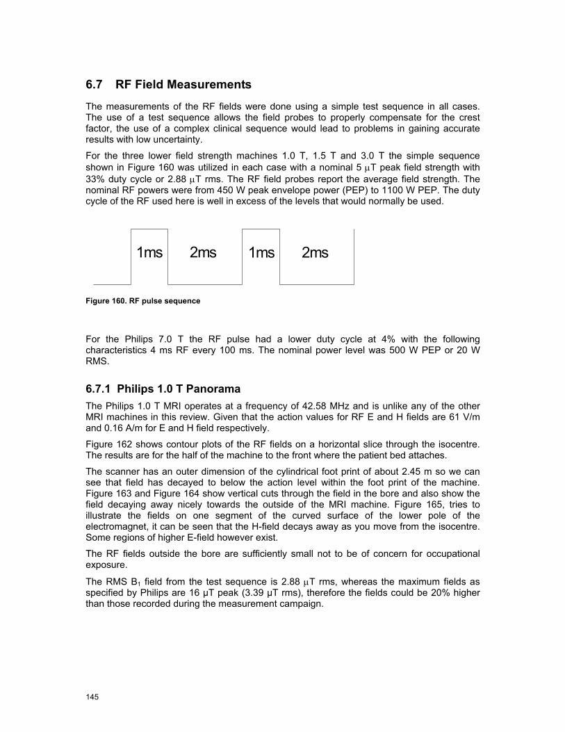
145
6.7 RF Field Measurements
The measurements of the RF fields were done using a simple test sequence in all cases. The use of a test sequence allows the field probes to properly compensate for the crest factor, the use of a complex clinical sequence would lead to problems in gaining accurate results with low uncertainty.
For the three lower field strength machines 1.0 T, 1.5 T and 3.0 T the simple sequence shown in Figure 160 was utilized in each case with a nominal 5 µT peak field strength with 33% duty cycle or 2.88 µT rms. The RF field probes report the average field strength. The nominal RF powers were from 450 W peak envelope power (PEP) to 1100 W PEP. The duty cycle of the RF used here is well in excess of the levels that would normally be used.
1ms 2ms 1ms 2ms
Figure 160. RF pulse sequence
For the Philips 7.0 T the RF pulse had a lower duty cycle at 4% with the following characteristics 4 ms RF every 100 ms. The nominal power level was 500 W PEP or 20 W RMS.
6.7.1 Philips 1.0 T Panorama The Philips 1.0 T MRI operates at a frequency of 42.58 MHz and is unlike any of the other MRI machines in this review. Given that the action values for RF E and H fields are 61 V/m and 0.16 A/m for E and H field respectively.
Figure 162 shows contour plots of the RF fields on a horizontal slice through the isocentre. The results are for the half of the machine to the front where the patient bed attaches.
The scanner has an outer dimension of the cylindrical foot print of about 2.45 m so we can see that field has decayed to below the action level within the foot print of the machine. Figure 163 and Figure 164 show vertical cuts through the field in the bore and also show the field decaying away nicely towards the outside of the MRI machine. Figure 165, tries to illustrate the fields on one segment of the curved surface of the lower pole of the electromagnet, it can be seen that the H-field decays away as you move from the isocentre. Some regions of higher E-field however exist.
The RF fields outside the bore are sufficiently small not to be of concern for occupational exposure.
The RMS B1 field from the test sequence is 2.88 µT rms, whereas the maximum fields as specified by Philips are 16 µT peak (3.39 µT rms), therefore the fields could be 20% higher than those recorded during the measurement campaign.
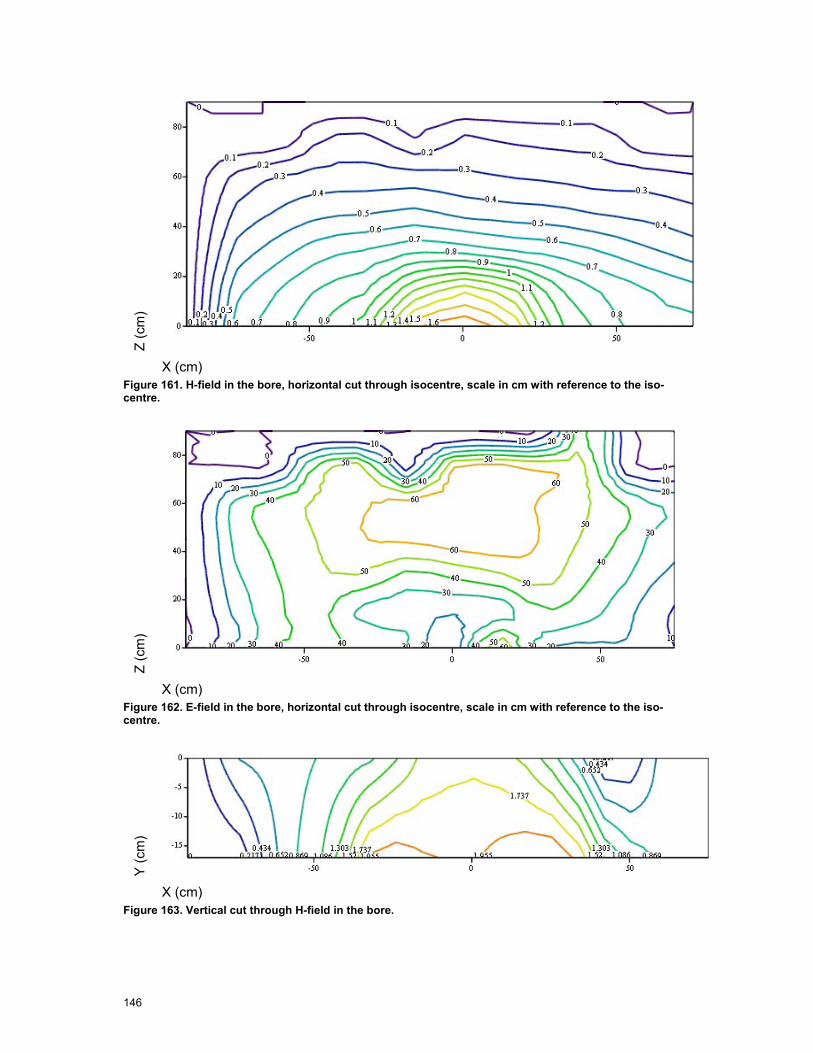
146
Z (c
m)
X (cm) Figure 161. H-field in the bore, horizontal cut through isocentre, scale in cm with reference to the iso-centre.
Z (c
m)
X (cm) Figure 162. E-field in the bore, horizontal cut through isocentre, scale in cm with reference to the iso-centre.
Y (c
m)
X (cm) Figure 163. Vertical cut through H-field in the bore.

147
Y (c
m)
X (cm) Figure 164. Vertical cut through E-field in the bore.
As a worker leans into the MRI machine to check a patient or perform interventional MRI it is likely that they will lean on the curved surface of the MRI machine, it is therefore important to gain an understanding of the fields that are present on the surface. Figure 55 shows how the measurement positions are located with respect to the scanner and Figure 165 shows the measured values. The colour of the dots represent the magnitude of the field at the measurement points, whilst the positions of the dots represent the locations as viewed from above.
A/m
V/m
Figure 165. RF fields on the lower curved surface of the MRI, H and E-field respectively (A/m, V/m)

148
The fields on the bore show enhanced values for the H-field close to the supporting pillar and E-field along the edge of the bed.
6.7.2 Siemens 1.5 T Avanto The Siemens 1.5 T MRI machine operates at ~64 MHz, the RF field decays away relatively rapidly, as can be seen in Figure 166 and Figure 167 for E and H-field respectively. It can be seen that even just in front of the MRI bore the E-field is well below the action value of 61 V/m for the test RF sequence, the H-field does exceed the 0.16 A/m action value immediately in front of the machine, but has decayed to 33% or less of the action value by some 20 cm in front of the face of the machine.
The RMS B1 field from the test sequence is 2.88 µT RMS, where as the maximum fields as specified by Siemens are 30 µT peak (23.5 µT guaranteed for all loads) with 4% duty cycle which correspond to 6 µT RMS (4.7 µT RMS), therefore the fields could be 208% higher than those recorded during the measurement campaign. Taking this into account the E-field remains below the action value and the H-field exceeds the value immediately in front of the machine, but 15 cm away it is reduced to below the value.
Figure 166. E-field outside the bore (V/m).

149
Figure 167. H-Field outside the bore (A/m)

150
X (c
m)
Horizontal cut
Z (cm)
Y (c
m)
Vertical cut
Z (cm) Figure 168. RF H-Field in the bore (A/m). Scale in cm.
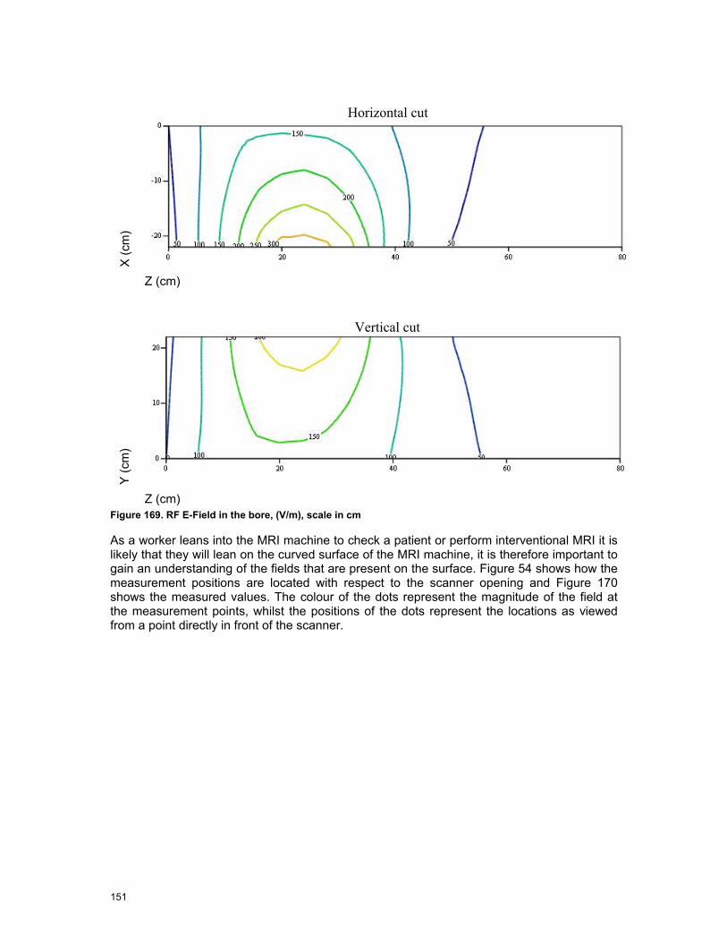
151
X (c
m)
Horizontal cut
Z (cm)
Y (c
m)
Vertical cut
Z (cm) Figure 169. RF E-Field in the bore, (V/m), scale in cm
As a worker leans into the MRI machine to check a patient or perform interventional MRI it is likely that they will lean on the curved surface of the MRI machine, it is therefore important to gain an understanding of the fields that are present on the surface. Figure 54 shows how the measurement positions are located with respect to the scanner opening and Figure 170 shows the measured values. The colour of the dots represent the magnitude of the field at the measurement points, whilst the positions of the dots represent the locations as viewed from a point directly in front of the scanner.
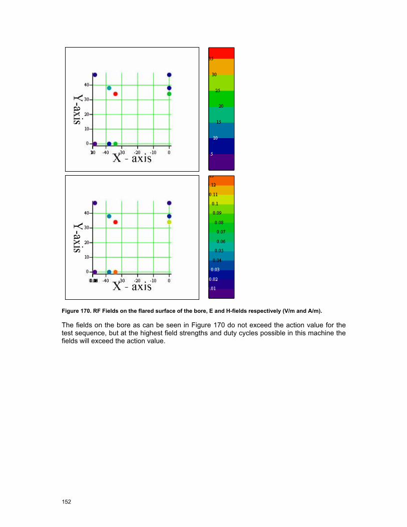
152
Figure 170. RF Fields on the flared surface of the bore, E and H-fields respectively (V/m and A/m).
The fields on the bore as can be seen in Figure 170 do not exceed the action value for the test sequence, but at the highest field strengths and duty cycles possible in this machine the fields will exceed the action value.
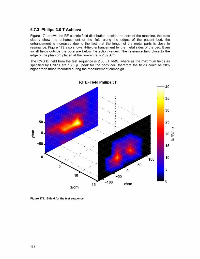
153
6.7.3 Philips 3.0 T Achieva Figure 171 shows the RF electric field distribution outside the bore of the machine, the plots clearly show the enhancement of the field along the edges of the patient bed, the enhancement is increased due to the fact that the length of the metal parts is close to resonance. Figure 172 also shows H-field enhancement by the metal sides of the bed. Even so all fields outside the bore are below the action values. The reference field close to the edge of the phantom placed at the iso-centre is 2.09 A/m.
The RMS B1 field from the test sequence is 2.88 µT RMS, where as the maximum fields as specified by Philips are 13.5 µT peak for the body coil, therefore the fields could be 20% higher than those recorded during the measurement campaign.
Figure 171. E-field for the test sequence.
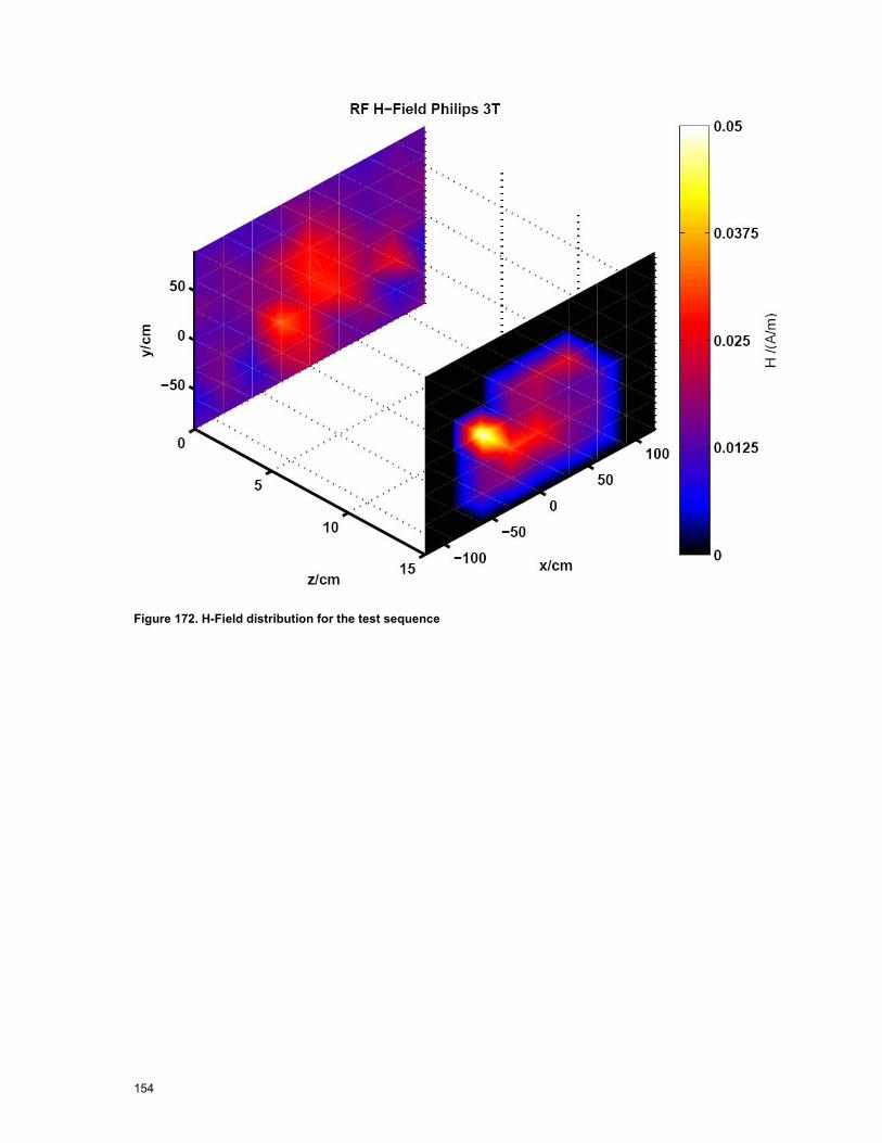
154
Figure 172. H-Field distribution for the test sequence

155
X (c
m)
Horizontal cut
Z (cm)
Y (c
m)
Vertical cut
Z (cm) Figure 173. E-Field in the bore (V/m), scales in cm

156
X (c
m)
Horizontal cut
Z (cm)
Y (c
m)
Vertical cut
Z (cm) Figure 174. H-field in the bore (A/m), scales in cm.
As a worker leans into the MRI machine to check a patient or perform interventional MRI it is likely that they will lean on the curved surface of the MRI machine, it is therefore important to gain an understanding of the fields that are present on the surface. Figure 54 shows how the measurement positions are located with respect to the scanner opening and Figure 175 shows the measured values. The colour of the dots represent the magnitude of the field at the measurement points, whilst the positions of the dots represent the locations as viewed from a point directly in front of the scanner.

157
Figure 175. RF Fields on the flared surface of the bore, E and H-fields respectively (V/m and A/m).
The fields on the flared opening of the bore of the machine do not exceed the action values.
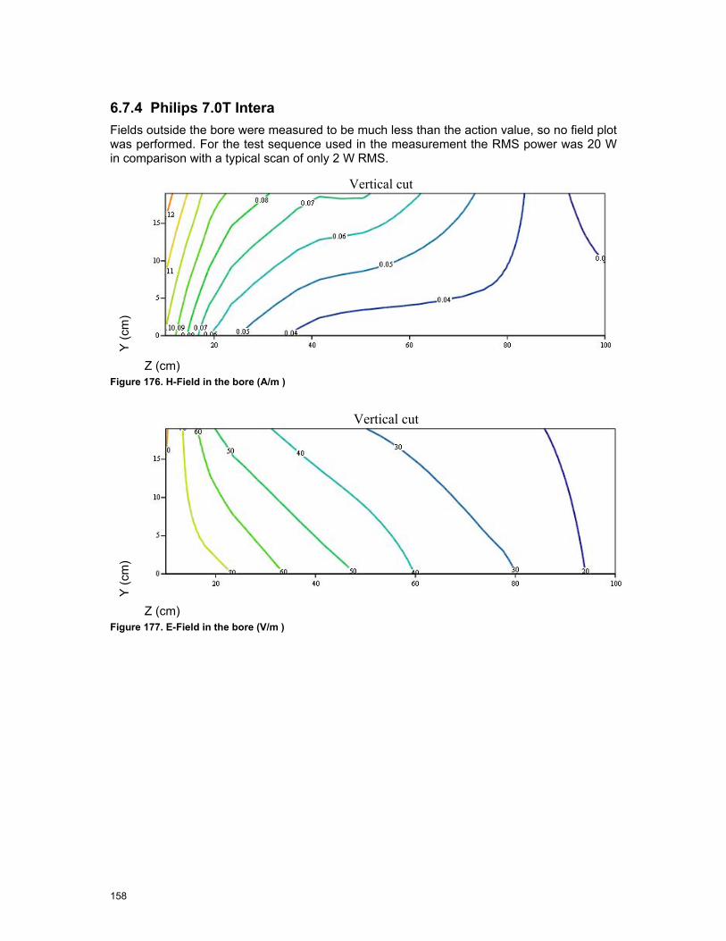
158
6.7.4 Philips 7.0T Intera Fields outside the bore were measured to be much less than the action value, so no field plot was performed. For the test sequence used in the measurement the RMS power was 20 W in comparison with a typical scan of only 2 W RMS.
Y (c
m)
Vertical cut
Z (cm) Figure 176. H-Field in the bore (A/m )
Y (c
m)
Vertical cut
Z (cm) Figure 177. E-Field in the bore (V/m )
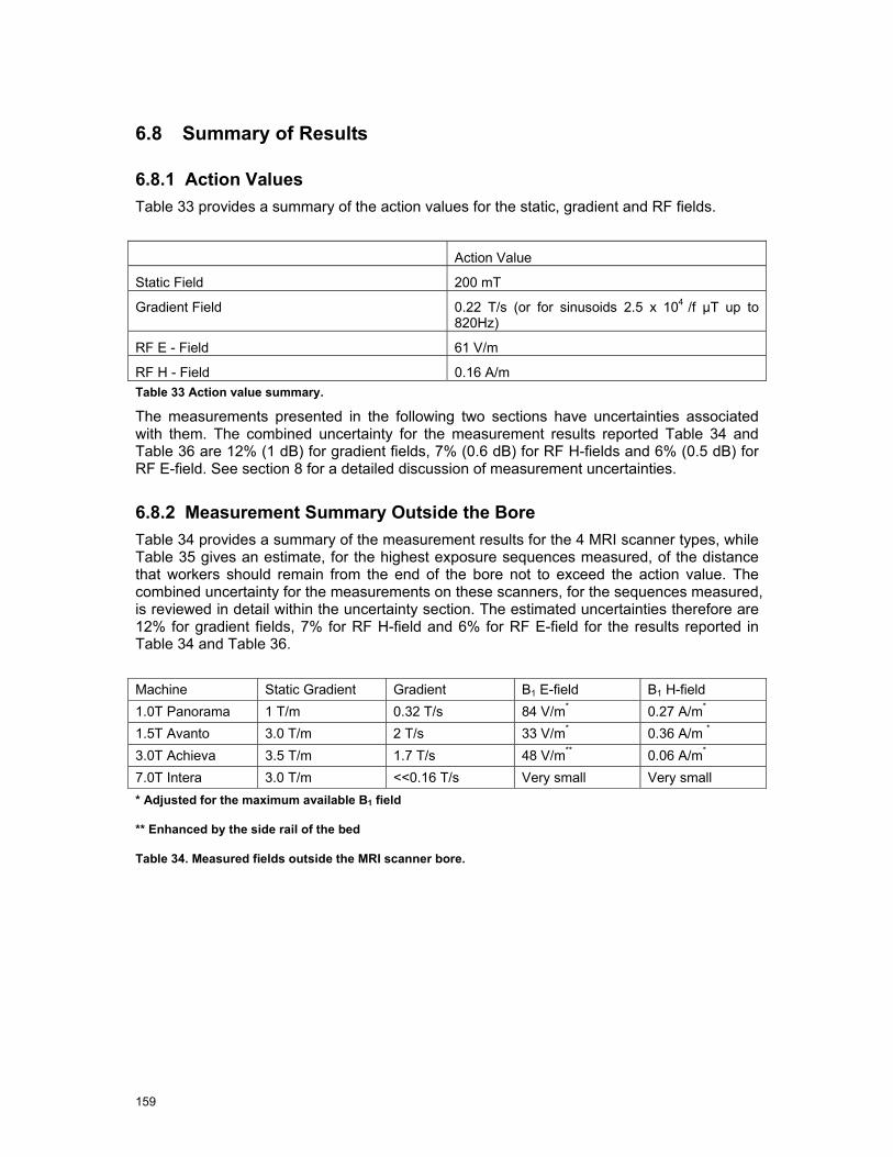
159
6.8 Summary of Results
6.8.1 Action Values Table 33 provides a summary of the action values for the static, gradient and RF fields.
Action Value
Static Field 200 mT
Gradient Field 0.22 T/s (or for sinusoids 2.5 x 10⁴ /f µT up to 820Hz)
RF E - Field 61 V/m
RF H - Field 0.16 A/m Table 33 Action value summary.
The measurements presented in the following two sections have uncertainties associated with them. The combined uncertainty for the measurement results reported Table 34 and Table 36 are 12% (1 dB) for gradient fields, 7% (0.6 dB) for RF H-fields and 6% (0.5 dB) for RF E-field. See section 8 for a detailed discussion of measurement uncertainties.
6.8.2 Measurement Summary Outside the Bore Table 34 provides a summary of the measurement results for the 4 MRI scanner types, while Table 35 gives an estimate, for the highest exposure sequences measured, of the distance that workers should remain from the end of the bore not to exceed the action value. The combined uncertainty for the measurements on these scanners, for the sequences measured, is reviewed in detail within the uncertainty section. The estimated uncertainties therefore are 12% for gradient fields, 7% for RF H-field and 6% for RF E-field for the results reported in Table 34 and Table 36.
Machine Static Gradient Gradient B1 E-field B1 H-field 1.0T Panorama 1 T/m 0.32 T/s 84 V/m* 0.27 A/m* 1.5T Avanto 3.0 T/m 2 T/s 33 V/m* 0.36 A/m *
3.0T Achieva 3.5 T/m 1.7 T/s 48 V/m** 0.06 A/m* 7.0T Intera 3.0 T/m <<0.16 T/s Very small Very small * Adjusted for the maximum available B1 field
** Enhanced by the side rail of the bed
Table 34. Measured fields outside the MRI scanner bore.
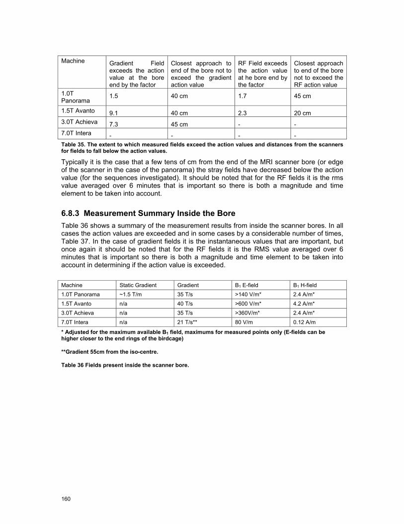
160
Machine Gradient Field
exceeds the action value at the bore end by the factor
Closest approach to end of the bore not to exceed the gradient action value
RF Field exceeds the action value at he bore end by the factor
Closest approach to end of the bore not to exceed the RF action value
1.0T Panorama
1.5 40 cm 1.7 45 cm
1.5T Avanto 9.1 40 cm 2.3 20 cm 3.0T Achieva 7.3 45 cm - - 7.0T Intera - - - - Table 35. The extent to which measured fields exceed the action values and distances from the scanners for fields to fall below the action values.
Typically it is the case that a few tens of cm from the end of the MRI scanner bore (or edge of the scanner in the case of the panorama) the stray fields have decreased below the action value (for the sequences investigated). It should be noted that for the RF fields it is the rms value averaged over 6 minutes that is important so there is both a magnitude and time element to be taken into account.
6.8.3 Measurement Summary Inside the Bore Table 36 shows a summary of the measurement results from inside the scanner bores. In all cases the action values are exceeded and in some cases by a considerable number of times, Table 37. In the case of gradient fields it is the instantaneous values that are important, but once again it should be noted that for the RF fields it is the RMS value averaged over 6 minutes that is important so there is both a magnitude and time element to be taken into account in determining if the action value is exceeded.
Machine Static Gradient Gradient B1 E-field B1 H-field 1.0T Panorama ~1.5 T/m 35 T/s >140 V/m* 2.4 A/m* 1.5T Avanto n/a 40 T/s >600 V/m* 4.2 A/m* 3.0T Achieva n/a 35 T/s >360V/m* 2.4 A/m* 7.0T Intera n/a 21 T/s** 80 V/m 0.12 A/m
* Adjusted for the maximum available B1 field, maximums for measured points only (E-fields can be higher closer to the end rings of the birdcage)
**Gradient 55cm from the iso-centre.
Table 36 Fields present inside the scanner bore.
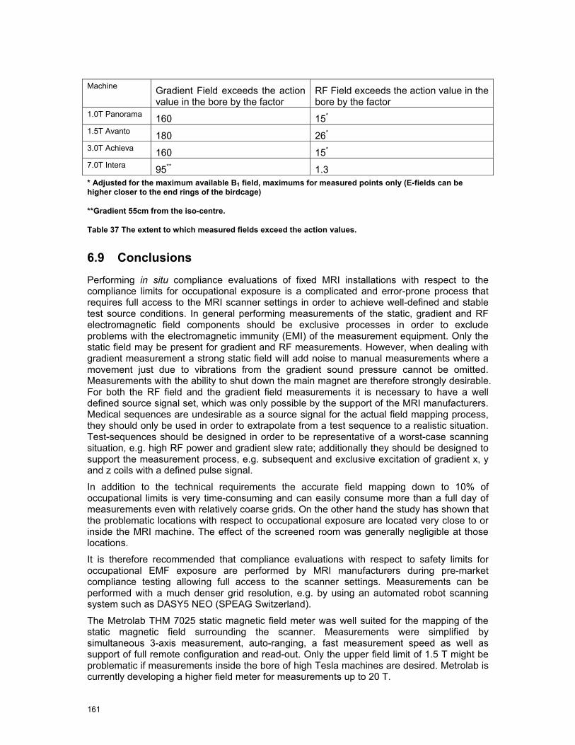
161
Machine Gradient Field exceeds the action
value in the bore by the factor RF Field exceeds the action value in the bore by the factor
1.0T Panorama 160 15*
1.5T Avanto 180 26*
3.0T Achieva 160 15*
7.0T Intera 95** 1.3 * Adjusted for the maximum available B1 field, maximums for measured points only (E-fields can be higher closer to the end rings of the birdcage)
**Gradient 55cm from the iso-centre.
Table 37 The extent to which measured fields exceed the action values.
6.9 Conclusions
Performing in situ compliance evaluations of fixed MRI installations with respect to the compliance limits for occupational exposure is a complicated and error-prone process that requires full access to the MRI scanner settings in order to achieve well-defined and stable test source conditions. In general performing measurements of the static, gradient and RF electromagnetic field components should be exclusive processes in order to exclude problems with the electromagnetic immunity (EMI) of the measurement equipment. Only the static field may be present for gradient and RF measurements. However, when dealing with gradient measurement a strong static field will add noise to manual measurements where a movement just due to vibrations from the gradient sound pressure cannot be omitted. Measurements with the ability to shut down the main magnet are therefore strongly desirable. For both the RF field and the gradient field measurements it is necessary to have a well defined source signal set, which was only possible by the support of the MRI manufacturers. Medical sequences are undesirable as a source signal for the actual field mapping process, they should only be used in order to extrapolate from a test sequence to a realistic situation. Test-sequences should be designed in order to be representative of a worst-case scanning situation, e.g. high RF power and gradient slew rate; additionally they should be designed to support the measurement process, e.g. subsequent and exclusive excitation of gradient x, y and z coils with a defined pulse signal.
In addition to the technical requirements the accurate field mapping down to 10% of occupational limits is very time-consuming and can easily consume more than a full day of measurements even with relatively coarse grids. On the other hand the study has shown that the problematic locations with respect to occupational exposure are located very close to or inside the MRI machine. The effect of the screened room was generally negligible at those locations.
It is therefore recommended that compliance evaluations with respect to safety limits for occupational EMF exposure are performed by MRI manufacturers during pre-market compliance testing allowing full access to the scanner settings. Measurements can be performed with a much denser grid resolution, e.g. by using an automated robot scanning system such as DASY5 NEO (SPEAG Switzerland).
The Metrolab THM 7025 static magnetic field meter was well suited for the mapping of the static magnetic field surrounding the scanner. Measurements were simplified by simultaneous 3-axis measurement, auto-ranging, a fast measurement speed as well as support of full remote configuration and read-out. Only the upper field limit of 1.5 T might be problematic if measurements inside the bore of high Tesla machines are desired. Metrolab is currently developing a higher field meter for measurements up to 20 T.

162
Instruments such as the Narda ELT400 are not well suited to the measurements of gradient fields due to the unequal steps between ranges, the ranges are 32 µT, 320 µT, 8 mT and 80 mT. The 25 fold step between 320 µT and 8 mT can result in signal sequences where the available signal to noise is not adequate. In addition when this instrument is used to record the actual pulse sequences it is not possible to automatically log which range was used for any given measurement, therefore it is not appropriate for automatic measurement procedures.
The RF field measurement probes and data logging system EASY4MRI of SPEAG Switzerland was well suited for the measurement of the RF fields. The system provides an excellent EMI against to gradient and static fields, full de-coupling of the probes and the data logger through optical data transmission as well as full remote interface for automated measurements. The dynamic range from <<10% to >100 times the action as well as an very small averaging volume of the isotropic E and H sensors makes the system well suited for the automated mapping of the RF electromagnetic fields.


164
7 Assessment of Induced Fields
7.1 Introduction
The experimental evaluation of the electromagnetic fields in the environment of several MRI scanners showed that the action values as posed by ICNIRP and stated in directive 2004/40/EC are exceeded in several cases. The actual analysis of the induced dosimetric quantities (current density, E-field and SAR) carried out by numerical means is presented in this section for the following typical occupational scenarios and scanners:
• Philips Achieva 3.0 T – exposure to time varying gradient fields
• Siemens Avanto 1.5 T– - exposure to both RF and time varying gradient fields
• Philips Panorama 1.0 T - Radiologist fixing breast clips – Exposure to both RF and time varying gradient fields
The scanners are modelled according to the information on coil design as provided by the manufacturers. Certain compromises were necessary because not all details of the scanners were disclosed. The impact of these compromises is discussed in Section 8.6 – 8.8and 9.4. For the validation of the numerical models, the experimentally assessed RF and gradient field distributions were used. In addition to the scenarios listed above, the induced currents due to movements through static fields are discussed for a generic solenoid. Since no geometrical or electrical data were available, a generic design had to be chosen based on average dimensions. The field gradients of the generic solenoid were normalized to measured results.
For the numerical analyses of the exposure, different simulation techniques for static, low frequency and RF exposure assessments were applied, which allows the mutual validation of the numerical results. In addition to a standard voxel model of the human body, several of the most advanced anatomical models developed within the Virtual Family Project were applied (Christ et al., 2008 [80]). After an overview of the present state of research and of the applied numerical techniques, the numerical models of the scanners are discussed and the exposure scenarios listed above are analyzed according to the incident fields as determined experimentally. Similar results suggesting non-compliance with limits prescribed in the Directive have been predicted in numerical modelling work reported by Li et al (2007) [68], Crozier et al (2007) [26], and Wang et al (2008) [84].
7.2 Objectives
In detail, the objectives of this section are to
• review the current state of numerical evaluation of dosimetric quantities induced by MRI scanners
• evaluate occupational exposure for typical scenarios and extrapolate to maximum incident exposure conditions
• compare the exposure of these scenarios to basic restrictions
• identify limitations of existing techniques
• identify requirements on tools

165
7.3 Present State of Research
7.3.1 SAR Induced by RF Electromagnetic Fields Little information is available on the exposure of health care workers to RF fields of MRI scanners. Most studies investigate the exposure of patients undergoing MR examinations focusing particularly on hot spots in the patient (e. g., Nadobny 2007 [72], Cabot 2007[51]) or, in case of (Hand 2006 [64]), on the exposure of the fetus in the womb of a pregnant woman. The studies show consistent results with respect to whole body SAR and the local exposure. The ratio between the maximum 10 g peak spatial average SAR in certain hot spots and the whole body SAR can easily exceed 10 dB. All relevant studies use the Finite-Difference Time-Domain (FDTD) method or the Finite Integration Technique (FIT) to quantify the exposure of anatomical patient models (whole or partial body) by the fields of the birdcage coil.
7.3.2 Currents due to Time Varying Gradient Fields The prevailing literature on the numerical evaluation of currents induced in the body due to gradient stimulation deals with the exposure of the patient (Liu et al, 2003 [69], So et al, 2004 [75] , Bencsik et al, 2007 [50]). Since the fields of the coils applied in these studies are only well characterized inside the bore, the extrapolation of the findings to assess occupational exposure is not straightforward. Different ways of normalization used by different authors often render the comparison of the results difficult. (So et al, 2004 [75]) point out the necessity of reporting the location at which dB/dt is measured.
Liu et al, 2003 [69] report maximum induced current densities of 0.28 A/m² in a patient model at dB/dt of 22 T/s. Significantly higher values of up to 2.5 A/m² for a dB/dt of 48 T/s are found by (Bencsik et al, 2007 [50]). The authors note that their results generally exceed those of other studies and attribute this to a comparatively large volume within which the field gradients of their coil models remain constant.
The induced currents in body models standing next to gradient coils are discussed in a study by Chadwick in 2007 [52] who reports maximum induced maximum induced current densities of more than 24 mA/m² for superimposed fields of the x-, y- and z-gradient coil at 1 mT/m (per coil) at a frequency of 1 kHz. Body average values of 5.5 mA/m² are reported. According to (Chadwick 2007 [52]), applying these results to a typical field gradient of 40 mT/m and considering the harmonic components of a pulse of 0.25 ms rise time requires scaling of the induced currents by a factor of 32. This exceeds the ICNIRP limit of 10 mA/m² RMS (1 kHz).
An experimental evaluation of the field strength on the skin caused by gradient fields is carried out in (Glover and Bowtell, 2008 [63]). The authors find that the comparison of their results with those of the studies cited above is difficult because of the different ways of normalizing and presenting the data, yet they conclude that the main findings of the numerical studies are “not dissimilar” to their measured worst cases.
7.3.3 Currents due to Movements in Static Fields A recent publication by (Crozier, 2007 [53]), which extends earlier work by the same research group (Liu et al, 2003 [69], Crozier et Liu, 2005 [54]) discusses the induced electrical field strengths and current densities in two anatomical body models (adult male and female) moving in the vicinity of different magnets (1.5 T, 4.0 T and 7.0 T) at velocities of 1 m/s at different directions and positions. The induced field quantities were calculated using a finite difference technique to determine the scalar potential Φ for a given magnetic field in motion. The study reports current density maxima which exceed the basic restrictions of 57 mA/m² (40 mA/m² RMS) posed by ICNIRP by about a factor of 10. Average current densities are reported within the order of magnitude of the ICNIRP limit. The study further concluded that a direct correlation of the static field strength and the induced current densities cannot

166
be established. It largely depends on the field distribution around the magnet. Highest current densities are observed for motions in the z-direction immediately in front of the bore.
An experimental evaluation of current densities induced on the skin by exposure to switched gradient fields and movement through static fields using a particularly developed wearable sensor (Glover and Bowtell, 2008 [63]) reports induced current densities in the order of magnitude of 100 mA/m², which apparently confirms previous numerical studies.
7.4 Numerical Methods
7.4.1 RF Simulations using FDTD and FIT The finite-difference time-domain (FDTD) method and the finite integration technique (FIT) are based on the discretisation of Maxwell’s equations in their differential and integral form, respectively. The FDTD method expresses the differential Maxwell vector equations in scalar form relative to three orthogonal axes and these scalar equations are in turn approximated by finite difference equations. Discretisation involves spatially sampling the E and H field distributions on a staggered 3-dimensional grid over the volume of interest and over a period of time. FIT discretises Maxwell’s equations in integral form, and transforms them into a set of matrix equations, the Maxwell Grid Equations (MGEs), on an orthogonal dual grid pair (i. e. staggered grid). Electric grid voltages and magnetic facet fluxes are allocated to the first grid, whilst magnetomotive forces and electric facet fluxes are allocated to the second grid. In the time domain, both algorithms apply a leap-frog scheme to advance the field components on the grids in time. For staggered rectilinear grids, the numerical properties of the two methods are essentially the same.
Detailed discussion of the FIT can be found in Wust et al (1993) [82] , Weiland (1996) [79], Krietenstein et al (2003) [67], and Schuhmann and Weiland (2003) [83], and a summary can be in found in Hand et al (2006) [64]. The most comprehensive description of the FDTD method is found in Taflove and Hagness (2005)[76]. FDTD and FIT codes have been used in many MRI related studies of coil design, performance, and safety (eg Vaughan et al 1994 [77], Ibrahim et al 2001[66], Collins et al 2004 [56], Diehl et al (2005) [57], Hanus et al (2005) [65], Hand et al (2006) [64], and Nadobny et al (2007) [72]).
Within the framework of this project, we have used FDTD implementation of the commercial package SEMCAD X v.13.2 (Schmid & Partner Engineering AG, Zürich) and the transient FIT solver in the commercial package Microwave Studio v2008 (Computer Simulation Technology, Darmstadt).
7.4.2 Low Frequency Magnetic Fields
7.4.2.1 Finite Element Quasistatic Solver The first method we have used is the low frequency solver within SEMCAD X. In spite of the prominent role of the FDTD algorithm, at lower frequencies the method becomes inefficient due to the explicit time integration scheme. Using quasi-static approximations of Maxwell’s equations can lower the computational burden considerably. For the current project the magneto quasi-static approximation is the method of choice. The approximation neglects the displacement current. The criterion of a valid magneto quasi-static approximation is
d << λ

167
where d is the diagonal of the computational domain and the wavelength λ is calculated with the complex permittivity.
If in addition σ>>ω ε (ω = angular frequency), the equations simplify in frequency domain to a real valued linear system
div (σ grad Φ) = j ω div( σ A0 )
where A0 is the vector potential of the external coil configuration j0, Φ is the unknown scalar potential and the electric field is
E = -j ω A0+ grad Φ
and has vanishing real part, when A0 is real valued. The linear equation system is constructed with the finite element method (FEM) on a non-uniform rectilinear grid (same grid as FDTD simulations). The final linear system is solved with a sparse iterative solver package.
7.4.2.2 Frequency Scaling The second approach we have used is the scaled frequency method (Gandhi and Chen 1992 [62]), implemented within both the transient FDTD and FIT simulations. The simulation is carried out at a higher frequency (typically 1-5 MHz), but at which a quasi-static solution is still valid, and the tissue conductivity σ is taken to be that at the (low kHz) frequency of interest f . The induced E-field ( )z,y,xE′ at the simulation frequency f ′ is scaled to that at
the frequency of interest f , ( )z,y,xE using ( ) ( )z,y,xEffz,y,xE ′′
= . Likewise, the induced
current density ( )z,y,xJ at frequency f is found from the computed ( )z,y,xJ ′ at frequency
f ′ using ( ) ( )z,y,xJffz,y,xJ ′′
= . This method has been used previously in relation to MRI
related exposure to investigate peripheral nerve stimulation in a human body model positioned within a whole body gradient coil set (Collins et al 2002 [56]) as well as by ourselves in a recent publication regarding occupational exposure to time-varying gradient fields (Li et al 2007 [69]).
In the investigations reported here, the transient fields were simulated at 1 MHz and frequency scaling to 1 kHz was applied.
7.4.3 Movements through Static Fields
A similar derivation as in the previous section can be done for the situation of a lossy moving object in a static magnetic field. Instead of using the frame of reference of a moving object in a non-moving magnetic field, the reference system is chosen to be a non-moving object in a moving static field. Therefore, the vector potential A0(called simply A) is now moving, i.e.,

168
A(r) ==> A(r-vt)
and its time derivative for the x component yields
∂Ax/∂t = grad( Ax) · (-v)
∂Ay/∂t = grad( Ay) · (-v)
∂Az/∂t = grad( Az) · (-v)
(chain derivation rule). Therefore the final equations to solve read
div (σ grad Φ) = div( σ ∂A/∂t )
and the electric field becomes
E = -∂A/∂t + grad Φ.
Again, the final discretisation uses the FEM technique and the sparse linear iterative solvers described in Section 7.4.2.
7.5 Anatomical Models
7.5.1 The Virtual Family – CAD Models of the Human Body Conventional dosimetric models of the human body consist of prevoxeled data of a fixed resolution. In numerical simulations using the FDTD or FIT method, this generally determines their orientation in the computational grid as well as the mesh resolution. If the models need to be rotated in the computational domain, or if their resolution must be modified due to numerical reasons, this usually goes along with loss of accuracy due to multiple sampling, particularly with respect to small organs or thin tissue layers, such as the skin.
In order to overcome these disadvantages, eight whole body models (two adults and six children) were developed within the framework of the Virtual Family Project and a follow up study. The models are based on high resolution MRI scans (0.5 mm x 0.5 mm x 1.0 mm in the head, 0.9 mm x 0.9 mm x 2 mm in the trunk and the limbs) using a Siemens Avanto 1.5 T scanner. 84 tissues and organs were segmented using an in-house software and reconstructed as three-dimensional CAD objects yielding anatomical models of unprecedented fidelity and quality. These models can be arbitrarily placed in the grid and meshed at arbitrary resolution without loss of detail.
Figure 178 shows the three CAD models used for part of the simulations of this project. Table 38 summarizes their properties. Further details on the models and their development can be found in (Christ et al, 2008 [80]). Currently, a poser software is under development, which allows natural articulation of all limbs of the models.
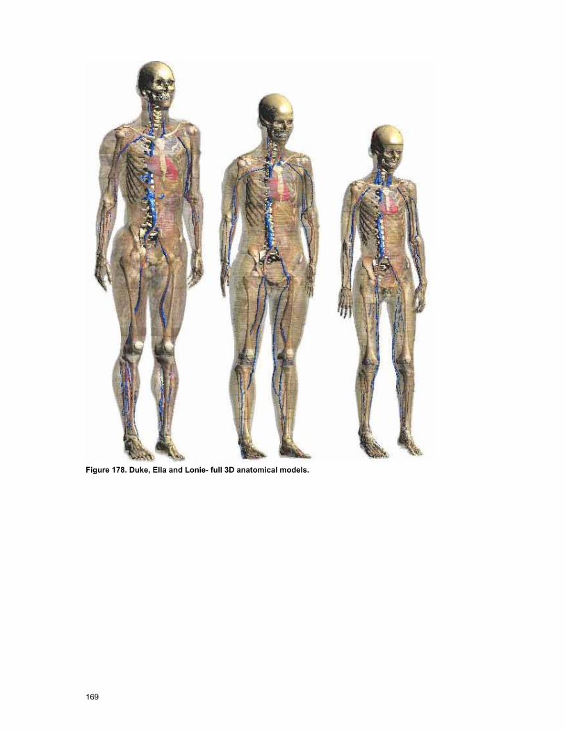
169
Figure 178. Duke, Ella and Lonie- full 3D anatomical models.
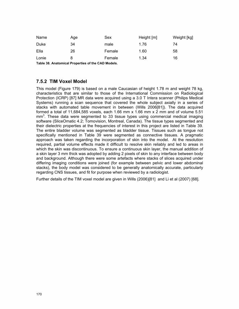
170
Name Age Sex Height [m] Weight [kg]
Duke 34 male 1.76 74
Ella 26 Female 1.60 58
Lonie 8 Female 1.34 16 Table 38. Anatomical Properties of the CAD Models.
7.5.2 TIM Voxel Model This model (Figure 179) is based on a male Caucasian of height 1.78 m and weight 78 kg, characteristics that are similar to those of the International Commission on Radiological Protection (ICRP) [87] MR data were acquired using a 3.0 T Intera scanner (Philips Medical Systems) running a scan sequence that covered the whole subject axially in a series of stacks with automated table movement in between (Wills 2006[81]). The data acquired formed a total of 11,684,585 voxels, each 1.66 mm x 1.66 mm x 2 mm and of volume 5.51 mm3. These data were segmented to 33 tissue types using commercial medical imaging software (SliceOmatic 4.2; Tomovision, Montreal, Canada). The tissue types segmented and their dielectric properties at the frequencies of interest in this project are listed in Table 39. The entire bladder volume was segmented as bladder tissue. Tissues such as tongue not specifically mentioned in Table 39 were segmented as connective tissues. A pragmatic approach was taken regarding the incorporation of skin into the model. At the resolution required, partial volume effects made it difficult to resolve skin reliably and led to areas in which the skin was discontinuous. To ensure a continuous skin layer, the manual addition of a skin layer 3 mm thick was adopted by adding 2 pixels of skin to any interface between body and background. Although there were some artefacts where stacks of slices acquired under differing imaging conditions were joined (for example between pelvic and lower abdominal stacks), the body model was considered to be generally anatomically accurate, particularly regarding CNS tissues, and fit for purpose when reviewed by a radiologist.
Further details of the TIM voxel model are given in Wills (2006)[81] and Li et al (2007) [68].
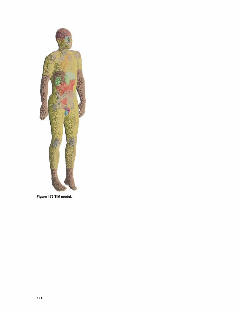
171
Figure 179 TIM model.
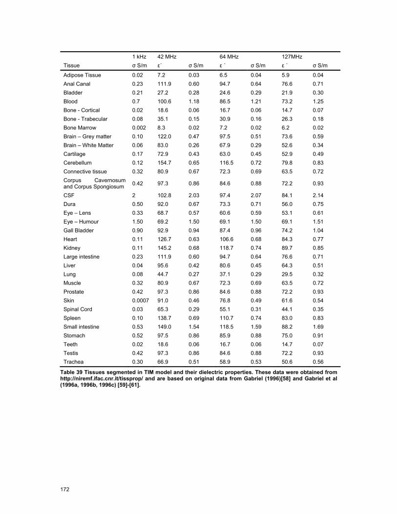
172
1 kHz 42 MHz 64 MHz 127MHz Tissue σ S/m ε´ σ S/m ε ´ σ S/m ε ´ σ S/m
Adipose Tissue 0.02 7.2 0.03 6.5 0.04 5.9 0.04 Anal Canal 0.23 111.9 0.60 94.7 0.64 76.6 0.71 Bladder 0.21 27.2 0.28 24.6 0.29 21.9 0.30 Blood 0.7 100.6 1.18 86.5 1.21 73.2 1.25 Bone - Cortical 0.02 18.6 0.06 16.7 0.06 14.7 0.07 Bone - Trabecular 0.08 35.1 0.15 30.9 0.16 26.3 0.18 Bone Marrow 0.002 8.3 0.02 7.2 0.02 6.2 0.02 Brain – Grey matter 0.10 122.0 0.47 97.5 0.51 73.6 0.59 Brain – White Matter 0.06 83.0 0.26 67.9 0.29 52.6 0.34 Cartilage 0.17 72.9 0.43 63.0 0.45 52.9 0.49 Cerebellum 0.12 154.7 0.65 116.5 0.72 79.8 0.83 Connective tissue 0.32 80.9 0.67 72.3 0.69 63.5 0.72 Corpus Cavernosum and Corpus Spongiosum 0.42 97.3 0.86 84.6 0.88 72.2 0.93
CSF 2 102.8 2.03 97.4 2.07 84.1 2.14 Dura 0.50 92.0 0.67 73.3 0.71 56.0 0.75 Eye – Lens 0.33 68.7 0.57 60.6 0.59 53.1 0.61 Eye – Humour 1.50 69.2 1.50 69.1 1.50 69.1 1.51 Gall Bladder 0.90 92.9 0.94 87.4 0.96 74.2 1.04 Heart 0.11 126.7 0.63 106.6 0.68 84.3 0.77 Kidney 0.11 145.2 0.68 118.7 0.74 89.7 0.85 Large intestine 0.23 111.9 0.60 94.7 0.64 76.6 0.71 Liver 0.04 95.6 0.42 80.6 0.45 64.3 0.51 Lung 0.08 44.7 0.27 37.1 0.29 29.5 0.32 Muscle 0.32 80.9 0.67 72.3 0.69 63.5 0.72 Prostate 0.42 97.3 0.86 84.6 0.88 72.2 0.93 Skin 0.0007 91.0 0.46 76.8 0.49 61.6 0.54 Spinal Cord 0.03 65.3 0.29 55.1 0.31 44.1 0.35 Spleen 0.10 138.7 0.69 110.7 0.74 83.0 0.83 Small intestine 0.53 149.0 1.54 118.5 1.59 88.2 1.69 Stomach 0.52 97.5 0.86 85.9 0.88 75.0 0.91 Teeth 0.02 18.6 0.06 16.7 0.06 14.7 0.07 Testis 0.42 97.3 0.86 84.6 0.88 72.2 0.93 Trachea 0.30 66.9 0.51 58.9 0.53 50.6 0.56
Table 39 Tissues segmented in TIM model and their dielectric properties. These data were obtained from http://niremf.ifac.cnr.it/tissprop/ and are based on original data from Gabriel (1996)[58] and Gabriel et al (1996a, 1996b, 1996c) [59]-[61].

173
7.6 MR Scanner Models and Validation
7.6.1 Philips 3.0 T Achieva
7.6.1.1 Gradient Fields
Figure 180 Achieva 3.0 T (courtesy of Philips Medical Systems) and axes used in modelling studies. The origin is taken to be the isocentre of the scanner.
Philips Medical Systems (Best, NL) provided detailed generic models of the x-, y-, and z-gradient coils of the 3.0 T Achieva (Figure 180) under a non-disclosure agreement.
The shielded z-gradient coil model consisted of 2 sets of concentric conducting loops, representing the primary and secondary coils. In a given set, the loops were of equal radius and their centres were distributed appropriately along the z-axis to produce a linear gradient in the central region of the coil. The magnitude of the current through all loops was constant but its direction within any particular loop depended upon the z-position of that loop relative to the centre of the coil sets.
The shielded x-gradient coil model consisted of sets of conducting loops that represented the primary and secondary coils. For each coil, these loops were located on a cylindrical surface and grouped into 4 quadrants. The cylindrical surfaces associated with primary and secondary coils were concentric but of differing radii. Currents of equal magnitude were impressed in each loop but the direction was dependent upon the coil and quadrant in which that loop was located. The shielded y-gradient coil set was similar to the x-gradient set except for a rotation of 90 degrees about the z-axis. The radii of the coils differed slightly to allow all coils (including the z-gradient coil set) to be positioned concentrically as is the case in the actual scanner.
Figure 181 shows the comparison between measured and (FS/FIT) simulated data for the total B-field both outside of the scanner bore. All data are referenced to gradients of 20.1 mT/m, the gradient used in the test measurement sequences. Simulated data are generally in satisfactory agreement with the relatively sparse measured data. Since the y-gradient set is similar to the x-gradient set but rotated by 90 degrees around the z-axis, some symmetry between off axis data for x- and y-coils is expected and this is reflected in both simulations and measurements. Figure 182 Achieva gradient fields calculated with SEMCAD X (Biot-Savart) normalized to 20.1 mT/m.shows the gradient fields of the same configuration calculated with the Biot-Savart solver of SEMCAD X.

174
Achieva 3T Z Gradient Coil Total B field versus axial distance from isocentre
0
50
100
150
200
250
300
0.9 1 1.1 1.2 1.3 1.4 1.5 1.6 1.7 1.8 1.9 2 2.1 2.2
Distance from isocentre z (m)
B fi
eld
(mic
roT)
x=0, y=0, z (Simulated) x=0, y=0, z (Measured)
Achieva 3T X and Y Gradient coils
Total B field versus axial distance from isocentre
0
100
200
300
400
500
600
0.9 1.1 1.3 1.5 1.7 1.9 2.1Distance from isocentre z (m)
B fi
eld
(mic
roT)
Xcoil x=0, y=0, z (Measured) Ycoil x=0, y=0, z (Measured) X-coil and y-coil x=0, y=0, z (Simulated)
X-coil x=-0.3, y=0, z (Measured) Y-coil x=0,y=-0.3, z (Measured) X-coil x=-0.3, y=0, z (Simulated)
X-coil x=0, y=-0.3, z (Measured) Y-Coil x=-.3, y=0, z (Measured) X-coil x=0, y=-0.3, z (Simulated)
Figure 181 Comparison of simulated (using frequency scaling/FIT method) and measured B-field profiles outside the scanner bore for the Achieva 3.0 T system. All data are scaled to 20.1 mT/m. Upper Figure: z-gradient coil. The data refer to profiles outside the bore along the central axis (x=0, y=0, z) Bottom Figure: x- and y-gradient coils. The data refer to profiles outside the bore along the central axis (x=0, y=0, z) and for two off-axis cases (x=0, y=0.3 m, z and x=-0.3 m, y=0, z). The simulated data shown for the x-gradient coil for x=-0. 3 m, y=0, z and x=0, y=0.3 m, z are also representative of y-gradient coil data for x=0, y=0.3 m, z and x=-0.3 m, y=0, z, respectively.
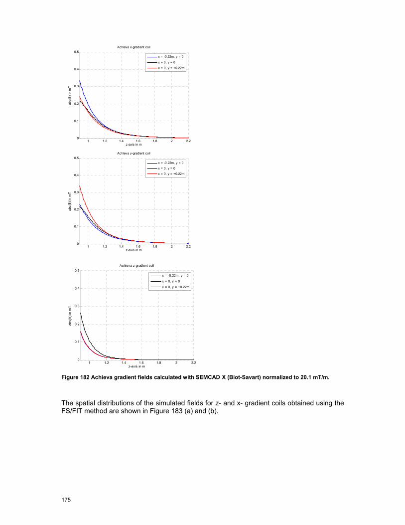
175
1 1.2 1.4 1.6 1.8 2 2.20
0.1
0.2
0.3
0.4
0.5
z-axis in m
abs(
B) i
n m
T
Achieva x-gradient coil
x = -0.22m, y = 0
x = 0, y = 0
x = 0, y = +0.22m
1 1.2 1.4 1.6 1.8 2 2.20
0.1
0.2
0.3
0.4
0.5
z-axis in m
abs(
B) i
n m
T
Achieva y-gradient coil
x = -0.22m, y = 0
x = 0, y = 0
x = 0, y = +0.22m
1 1.2 1.4 1.6 1.8 2 2.20
0.1
0.2
0.3
0.4
0.5
z-axis in m
abs(
B) i
n m
T
Achieva z-gradient coil
x = -0.22m, y = 0
x = 0, y = 0
x = 0, y = +0.22m
Figure 182 Achieva gradient fields calculated with SEMCAD X (Biot-Savart) normalized to 20.1 mT/m.
The spatial distributions of the simulated fields for z- and x- gradient coils obtained using the FS/FIT method are shown in Figure 183 (a) and (b).

176
Figure 183 (a) Spatial distribution of total B field (RMS) in y=0 plane due to Achieva z-gradient coil for z-values outside the scanner bore. The isocentric gradient is assumed to be 20.1 mT/m. Top: FS/FIT simulated data, Bottom: measured data (values in mT).
Figure 184 (b) Spatial distribution of total B field (RMS) in y=0 plane due to x-gradient coil for z-values outside the scanner bore. The isocentric gradient is assumed to be 40 mT/m.

177
7.6.2 Siemens 1.5T Avanto
Figure 185 Avanto 1.5 T (courtesy of Siemens Medical Solutions) showing axes used for modelling studies. The origin is at the isocentre of the scanner.
7.6.2.1 RF Fields
The RF body coil of the 1.5 T Avanto (Figure 185) was modelled as a 16 rung high pass circular cylindrical birdcage coil tuned to 64MHz through lumped capacitors incorporated within the structure. It was located concentrically within a cylindrical RF shield and driven in quadrature by applying RF signals simultaneously at 2 ports (in FIT models) or by assuming currents in the rungs with fixed phase differences between adjacent rungs (in FDTD models).
Figure 186 shows results of simulations using the FIT and FDTD techniques. The B1 field profiles for x=0, y=0, z show good agreement, as do those for x=0.16, y=0, z although in the latter case FIT predicted values close to the isocentre are larger than FDTD predicted values by approximately 1 %. Both methods predict that the E-field profiles are slightly asymmetric about the isocentre, reflecting an asymmetry in the numerical representation of the coil structure, although this is more enhanced in the FIT data than is the case for FDTD generated data. The E field profiles along x=0, y=0, z are in good agreement with values differing by up to 1.5 % (for z>0) and 6 % (for z<0). Along x=0.16 m, y=0, z the FIT predictions exceed those obtained using FDTD by up to 0.1 % (z>0) and 6 % (z<0). These differences in results obtained between FIT and FDTD may reflect the different ways in which the coil was excited in the respective models. In the case of the FIT model, voltages were applied in quadrature at the two ports and no restriction on the resulting currents in the coil structure was imposed. In the case of the FDTD model currents were imposed on the legs of the birdcage coil with equal phase differences between adjacent legs.
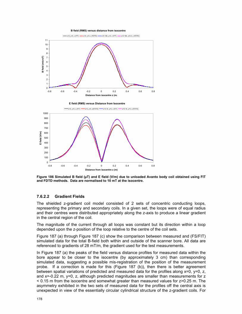
178
B field (RMS) versus distance from isocentre
0
1
2
3
4
5
6
7
8
9
10
11
-0.8 -0.6 -0.4 -0.2 0 0.2 0.4 0.6 0.8
Distance from isocentre z (m)
B fi
eld
(mic
roT)
x=0, y=0, z (FIT) x=0, y=0, z (FDTD) x=0.106, y=0, z (FIT) x=0.106, y=0.0, z (FDTD)
E field (RMS) versus Distance from Isocentre
0
100
200
300
400
500
600
700
800
900
1000
-0.8 -0.6 -0.4 -0.2 0 0.2 0.4 0.6 0.8
Distance from isocentre z (m)
E fie
ld (V
/m)
x=0, y=0, z (FIT) x=0, y=0, z(FDTD) x=0.16, y=0, z (FIT) x=0.16, y=0, z (FDTD)
Figure 186 Simulated B field (µT) and E field (V/m) due to unloaded Avanto body coil obtained using FIT and FDTD methods. Data are normalised to 10 mT at the isocentre.
7.6.2.2 Gradient Fields The shielded z-gradient coil model consisted of 2 sets of concentric conducting loops, representing the primary and secondary coils. In a given set, the loops were of equal radius and their centres were distributed appropriately along the z-axis to produce a linear gradient in the central region of the coil.
The magnitude of the current through all loops was constant but its direction within a loop depended upon the z-position of the loop relative to the centre of the coil sets.
Figure 187 (a) through Figure 187 (c) show the comparison between measured and (FS/FIT) simulated data for the total B-field both within and outside of the scanner bore. All data are referenced to gradients of 28 mT/m, the gradient used for the test measurements.
In Figure 187 (a) the peaks of the field versus distance profiles for measured data within the bore appear to be closer to the isocentre (by approximately 3 cm) than corresponding simulated data, suggesting a possible mis-registration of the position of the measurement probe. If a correction is made for this (Figure 187 (b)), then there is better agreement between spatial variations of predicted and measured data for the profiles along x=0, y=0, z, and x=-0.22 m, y=0, z, although predicted magnitudes are smaller than measurements for z < 0.15 m from the isocentre and somewhat greater than measured values for z>0.25 m. The asymmetry exhibited in the two sets of measured data for the profiles off the central axis is unexpected in view of the essentially circular cylindrical structure of the z-gradient coils. For
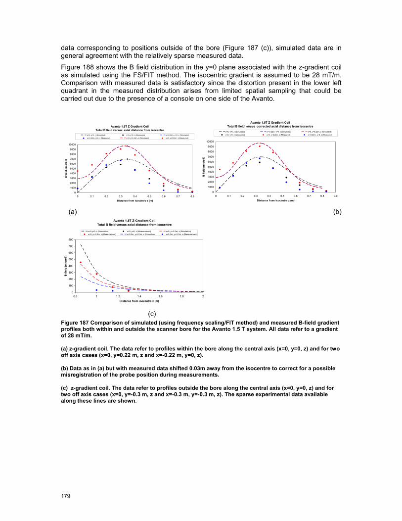
179
data corresponding to positions outside of the bore (Figure 187 (c)), simulated data are in general agreement with the relatively sparse measured data.
Figure 188 shows the B field distribution in the y=0 plane associated with the z-gradient coil as simulated using the FS/FIT method. The isocentric gradient is assumed to be 28 mT/m. Comparison with measured data is satisfactory since the distortion present in the lower left quadrant in the measured distribution arises from limited spatial sampling that could be carried out due to the presence of a console on one side of the Avanto.
Avanto 1.5T Z Gradient Coil Total B field versus axial distance from isocentre
0
1000
2000
3000
4000
5000
6000
7000
8000
9000
10000
0 0.1 0.2 0.3 0.4 0.5 0.6 0.7 0.8
Distance from isocentre z (m)
B fi
eld
(mic
roT)
x=0, y=0, z (Simulated) x=0, y=0, z (Measured) x=-0.22m, y=0, z (Simulated)x=-0.22m, y=0, z (Measured) x=0, y=0.22m, z (Simulated) x=0, y=0.22m, z (Measured)
Avanto 1.5T Z Gradient Coil Total B field versus corrected axial distance from isocentre
0
1000
2000
3000
4000
5000
6000
7000
8000
9000
10000
0 0.1 0.2 0.3 0.4 0.5 0.6 0.7 0.8 0.9
Distance from isocentre z (m)B
fiel
d (m
icro
T)
x=0, y=0, z (Simulated) x=-0.22m, y=0, z (Simulated) x=0, y=0.22m, z (Simulated)x=0, y=0, z (Measured) x=0, y=0.22m, z (Measured) x=-0.22m, y=0, z (Measured)
(a) (b)
Avanto 1.5T Z-Gradient Coil Total B field versus axial distance from isocentre
0
100
200
300
400
500
600
700
800
0.8 1 1.2 1.4 1.6 1.8 2
Distance from isocentre z (m)
B fi
eld
(mic
roT)
x=0,y=0, z (Simulation) x=0, y=0, z (Measurement) x=0, y=-0.3m, z (Simulation)x=0, y=-0.3m, z (Measurement) x=0.3m, y=-0.3m, z (Simulation) x=0.3m, y=-0.3m, z (Measurement)
(c) Figure 187 Comparison of simulated (using frequency scaling/FIT method) and measured B-field gradient profiles both within and outside the scanner bore for the Avanto 1.5 T system. All data refer to a gradient of 28 mT/m.
(a) z-gradient coil. The data refer to profiles within the bore along the central axis (x=0, y=0, z) and for two off axis cases (x=0, y=0.22 m, z and x=-0.22 m, y=0, z).
(b) Data as in (a) but with measured data shifted 0.03m away from the isocentre to correct for a possible misregistration of the probe position during measurements.
(c) z-gradient coil. The data refer to profiles outside the bore along the central axis (x=0, y=0, z) and for two off axis cases (x=0, y=-0.3 m, z and x=-0.3 m, y=-0.3 m, z). The sparse experimental data available along these lines are shown.
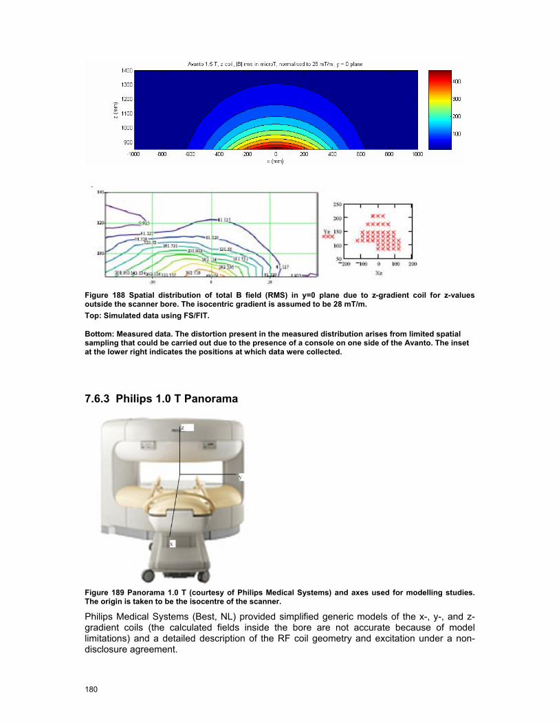
180
Figure 188 Spatial distribution of total B field (RMS) in y=0 plane due to z-gradient coil for z-values outside the scanner bore. The isocentric gradient is assumed to be 28 mT/m. Top: Simulated data using FS/FIT.
Bottom: Measured data. The distortion present in the measured distribution arises from limited spatial sampling that could be carried out due to the presence of a console on one side of the Avanto. The inset at the lower right indicates the positions at which data were collected.
7.6.3 Philips 1.0 T Panorama
Figure 189 Panorama 1.0 T (courtesy of Philips Medical Systems) and axes used for modelling studies. The origin is taken to be the isocentre of the scanner.
Philips Medical Systems (Best, NL) provided simplified generic models of the x-, y-, and z-gradient coils (the calculated fields inside the bore are not accurate because of model limitations) and a detailed description of the RF coil geometry and excitation under a non-disclosure agreement.
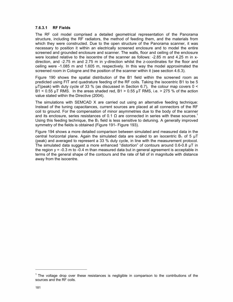
181
7.6.3.1 RF Fields The RF coil model comprised a detailed geometrical representation of the Panorama structure, including the RF radiators, the method of feeding them, and the materials from which they were constructed. Due to the open structure of the Panorama scanner, it was necessary to position it within an electrically screened enclosure and to model the entire screened and grounded enclosure and scanner. The walls, floor and ceiling of the enclosure were located relative to the isocentre of the scanner as follows: -2.85 m and 4.25 m in x-direction, and -2.75 m and 2.75 m in y-direction whilst the z-coordinates for the floor and ceiling were -1.085 m and 1.605 m, respectively. In this way the model approximated the screened room in Cologne and the position of the scanner within it (see section 4.6.3).
Figure 190 shows the spatial distribution of the B1 field within the screened room as predicted using FIT and quadrature feeding of the RF coils. Taking the isocentric B1 to be 5 µT(peak) with duty cycle of 33 % (as discussed in Section 6.7), the colour map covers 0 < B1 < 0.55 µT RMS. In the areas shaded red, B1 > 0.55 µT RMS, i.e. > 275 % of the action value stated within the Directive (2004).
The simulations with SEMCAD X are carried out using an alternative feeding technique: Instead of the tuning capacitances, current sources are placed at all connectors of the RF coil to ground. For the compensation of minor asymmetries due to the body of the scanner and its enclosure, series resistances of 0.1 Ω are connected in series with these sources.1 Using this feeding technique, the B1 field is less sensitive to detuning. A generally improved symmetry of the fields is obtained (Figure 191- Figure 193).
Figure 194 shows a more detailed comparison between simulated and measured data in the central horizontal plane. Again the simulated data are scaled to an isocentric B1 of 5 µT (peak) and averaged to represent a 33 % duty cycle, in line with the measurement protocol. The simulated data suggest a more enhanced “distortion” of contours around 0.6-0.8 µT in the region y = -0.3 m to -0.4 m than measured data but in general agreement is acceptable in terms of the general shape of the contours and the rate of fall of in magnitude with distance away from the isocentre.
1 The voltage drop over these resistances is negligible in comparison to the contributions of the sources and the RF coils.

182
Figure 190 FIT simulation of B1 field distribution for 1.0 T Panorama. Top: Plane y=0 (from rear to front of scanner through isocentre), Centre: Plane x=0 (from left to right through isocentre), Bottom: Plane z=0 (central horizontal plane). The white areas show the structure of the scanner. An isocentric B1 of 5 µT (peak) and duty cycle of 33 % is assumed. The colour map covers 0 < B1 < 0.55 µT RMS and in the areas shaded red B1 > 0.55 µT.

183
Figure 191 x-slice of B field in 1.0 T Panorama for a B1 in isocenter of 2.4 µT (measured value).
Figure 192 y-slice of B field in Panorama RF coil for a B1 in isocenter of 2.4 µT (measured value).
Figure 193 z-slice of B field in Panorama RF coil for a B1 in isocenter of 2.4 µT (measured value).

184
Figure 194. B1 field in central horizontal plane for an isocentric B1 of 5 µT (peak) and 33 % duty cycle. Left: Simulated data using FIT. Right: Measured data. In each figure, the horizontal axis represents left to right through the isocentre of the scanner and the vertical axis from the isocentre towards the patient couch.
7.6.3.2 Gradient Fields
The shielded z-gradient coil model consisted of 2 sets of concentric conducting loops, representing the primary and secondary coils. In a given set, the loops were of different radii and their centres were located along the z-axis to produce a linear gradient in the central region of the coil. The magnitude of the current through all loops within a given set was constant but its direction varied between loops.
The shielded x- and y-gradient coils were modelled as pairs of series of geometrically complex 3-dimensional loops.
Figure 195 compares measured and simulated data along the x-axis (from the isocentre towards the patient couch) for y=0 and z=0, y=0 and z =-0.17 m, y=0.15 m, z=0, and y=0.15 m z=-0.17 m. All data are scaled to a gradient of 16 mT/m, the gradient used during the test measurements. Measured and simulated data for y=0 and z=0 are in excellent agreement. However, in the z=-0.17 plane, measured data are significantly smaller than simulated values for x < 0.35 m, particularly around x ~ 0.2-0.25 m where the simulations suggest a peak in B field. The peak in the B-field is due to the limited number of turns in the simplified gradient coil model provided. Simulations of the gradient fields using the Biot-Savart solver of SEMCAD X show similar differences to the measurement results (Figure 200). Preliminary evaluations using simplified coil configurations suggest that these differences are due to the presence of the high permeability solenoid and the simplifications in the designs of the gradient coils supplied by Philips.
The predicted (using FS/FIT) and measured spatial distributions of the vertical gradient coil are compared in Figure 196 and Figure 197. Figure 196 shows simulated (using FS/FIT) and measured data for the x-component of B in the z=0 plane and in the quadrant x ≤ 0.6 m, y ≤ 0.6m whilst Figure 197 shows simulated (using FS/FIT) and measured data for the y-component of B, again in the z=0 plane and the quadrant x ≤ 0.6 m, y ≤ 0.6 m.
Figure 198 compares FS/FIT simulated and measured fields for the x-gradient coil along the x-axis (from the isocentre towards the patient couch) for y=0 and z=0, y=0 and z =-0.17 m, and y=0.15 m, z=0. All data are scaled to a gradient of 16 mT/m. Measured and simulated data for y=0, z=0 and y=0.15 m, z=0 are in excellent agreement. However, in the z=-0.17 m lane, measured data are significantly smaller than simulated values around x ~ 0.25-0.35 m where the simulations suggest a peak in B field this is due to the limited number of turns in the simplified gradient coil model provided.
Figure 199 shows the FS/FIT simulated and measured spatial distribution of the z-component of the field due to the x-gradient coil in the z=0 plane and within the quadrant x ≤ 0.6 m, y ≤ 0.6 m.
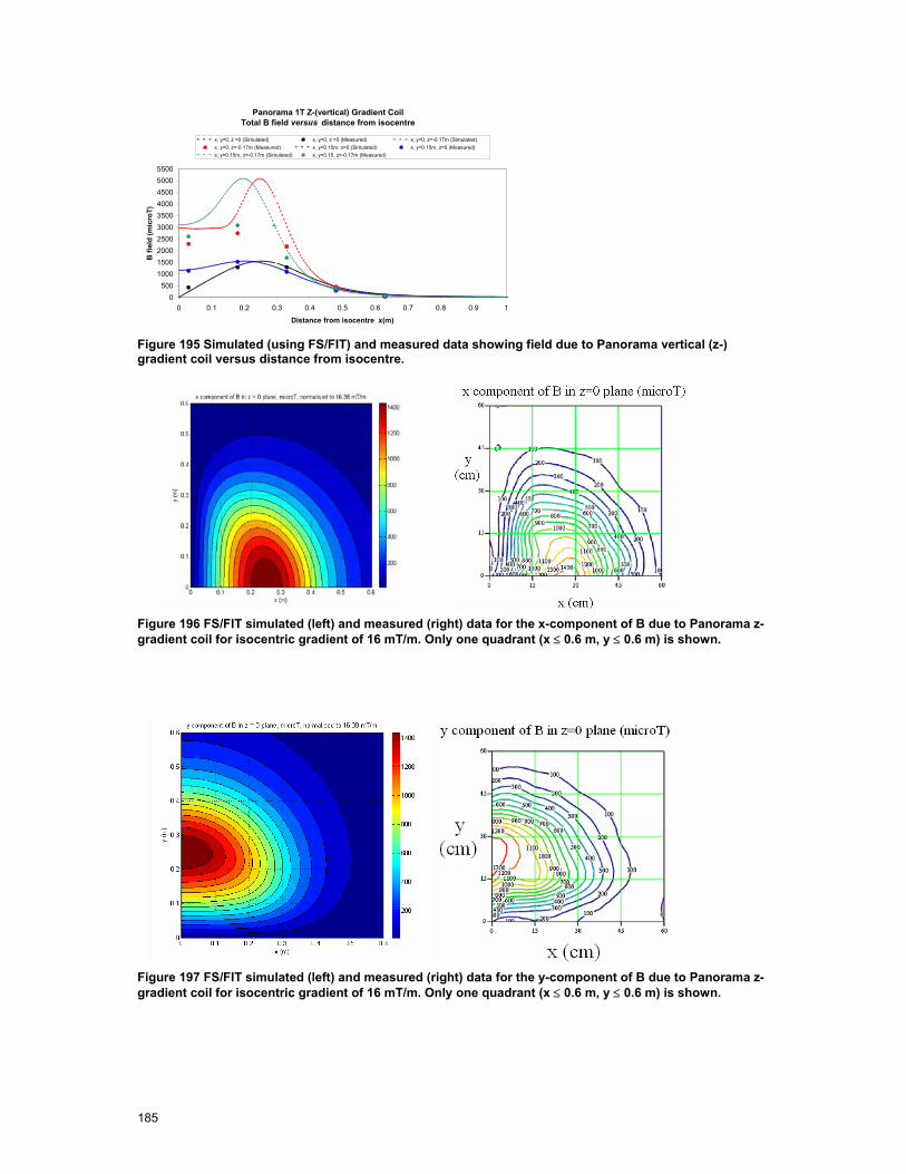
185
Panorama 1T Z-(vertical) Gradient Coil Total B field versus distance from isocentre
0500
1000150020002500300035004000450050005500
0 0.1 0.2 0.3 0.4 0.5 0.6 0.7 0.8 0.9 1
Distance from isocentre x(m)
B fi
eld
(mic
roT)
x, y=0, z =0 (Simulated) x, y=0, z =0 (Measured) x, y=0, z=-0.17m (Simulated)x, y=0, z=-0.17m (Measured) x, y=0.15m, z=0 (Simulated) x, y=0.15m, z=0 (Measured)x, y=0.15m, z=-0.17m (Simulated) x, y=0.15, z=-0.17m (Measured)
Figure 195 Simulated (using FS/FIT) and measured data showing field due to Panorama vertical (z-) gradient coil versus distance from isocentre.
Figure 196 FS/FIT simulated (left) and measured (right) data for the x-component of B due to Panorama z-gradient coil for isocentric gradient of 16 mT/m. Only one quadrant (x ≤ 0.6 m, y ≤ 0.6 m) is shown.
Figure 197 FS/FIT simulated (left) and measured (right) data for the y-component of B due to Panorama z-gradient coil for isocentric gradient of 16 mT/m. Only one quadrant (x ≤ 0.6 m, y ≤ 0.6 m) is shown.
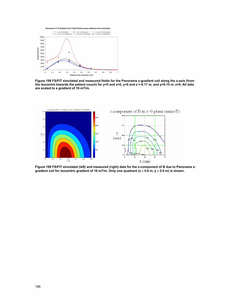
186
Panorama 1T X-Gradient Coil Total B field versus distance from isocentre
0
1000
2000
3000
4000
5000
6000
7000
8000
9000
10000
0 0.1 0.2 0.3 0.4 0.5 0.6 0.7 0.8 0.9 1
Distance from isocentre x (m)
B fi
eld
(mic
roT)
x, y=0, z=0 (Simulated) x, y=0, z=0 (Measured) x, y=0, z=-0.17m (Simulated)x, y=0, z=-0.17m (Measured) x, y=0.15m, z=0 (Simulated) x, y=0.15m, z=0 (Measured)
Figure 198 FS/FIT simulated and measured fields for the Panorama x-gradient coil along the x-axis (from the isocentre towards the patient couch) for y=0 and z=0, y=0 and z =-0.17 m, and y=0.15 m, z=0. All data are scaled to a gradient of 16 mT/m.
Figure 199 FS/FIT simulated (left) and measured (right) data for the z-component of B due to Panorama x-gradient coil for isocentric gradient of 16 mT/m. Only one quadrant (x ≤ 0.6 m, y ≤ 0.6 m) is shown.

187
0 0.1 0.2 0.3 0.4 0.5 0.6 0.7 0.8 0.9 10
2000
4000
6000
8000
10000
x-axis in m
abs(
B) i
n µ
T
Panorama x-gradient coil
y = 0, z = 0
y = 0, z = -0.17m
y = +0.15m, z = 0
0 0.1 0.2 0.3 0.4 0.5 0.6 0.7 0.8 0.9 10
2000
4000
6000
8000
10000
x-axis in m
abs(
B) i
n µ
T
Panorama y-gradient coil
y = 0, z = 0
y = 0, z = -0.17m
y = +0.15m, z = 0
0 0.1 0.2 0.3 0.4 0.5 0.6 0.7 0.8 0.9 10
2000
4000
6000
8000
10000
x-axis in m
abs(
B) i
n µ
T
Panorama z-gradient coil
y = 0, z = 0
y = 0, z = -0.17m
y = +0.15m, z = 0
y = +0.15m, z = -0.17m
Figure 200. Panorama gradient fields calculated with SEMCAD X (Biot-Savart) normalized to 16 mT/m.
0 0.1 0.2 0.3 0.4 0.5 0.6 0.7 0.8 0.9 10
2000
4000
6000
8000
10000
x-axis in m
abs(
B) i
n µ
T
Panorama x-gradient coil
y = 0, z = 0
y = 0, z = -0.17m
y = +0.15m, z = 0
0 0.1 0.2 0.3 0.4 0.5 0.6 0.7 0.8 0.9 10
2000
4000
6000
8000
10000
x-axis in m
abs(
B) i
n µ
T
Panorama y-gradient coil
y = 0, z = 0
y = 0, z = -0.17m
y = +0.15m, z = 0
0 0.1 0.2 0.3 0.4 0.5 0.6 0.7 0.8 0.9 10
2000
4000
6000
8000
10000
x-axis in m
abs(
B) i
n µ
T
Panorama z-gradient coil
y = 0, z = 0
y = 0, z = -0.17m
y = +0.15m, z = 0
y = +0.15m, z = -0.17m
Figure 201. Panorama gradient fields calculated with SEMCAD X (Biot-Savart) normalized to 16 mT/m.
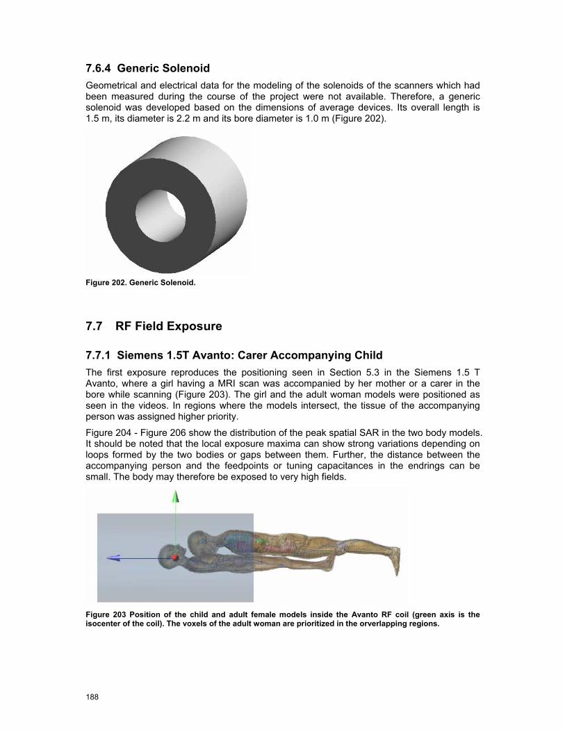
188
7.6.4 Generic Solenoid Geometrical and electrical data for the modeling of the solenoids of the scanners which had been measured during the course of the project were not available. Therefore, a generic solenoid was developed based on the dimensions of average devices. Its overall length is 1.5 m, its diameter is 2.2 m and its bore diameter is 1.0 m (Figure 202).
Figure 202. Generic Solenoid.
7.7 RF Field Exposure
7.7.1 Siemens 1.5T Avanto: Carer Accompanying Child The first exposure reproduces the positioning seen in Section 5.3 in the Siemens 1.5 T Avanto, where a girl having a MRI scan was accompanied by her mother or a carer in the bore while scanning (Figure 203). The girl and the adult woman models were positioned as seen in the videos. In regions where the models intersect, the tissue of the accompanying person was assigned higher priority.
Figure 204 - Figure 206 show the distribution of the peak spatial SAR in the two body models. It should be noted that the local exposure maxima can show strong variations depending on loops formed by the two bodies or gaps between them. Further, the distance between the accompanying person and the feedpoints or tuning capacitances in the endrings can be small. The body may therefore be exposed to very high fields.
Figure 203 Position of the child and adult female models inside the Avanto RF coil (green axis is the isocenter of the coil). The voxels of the adult woman are prioritized in the orverlapping regions.
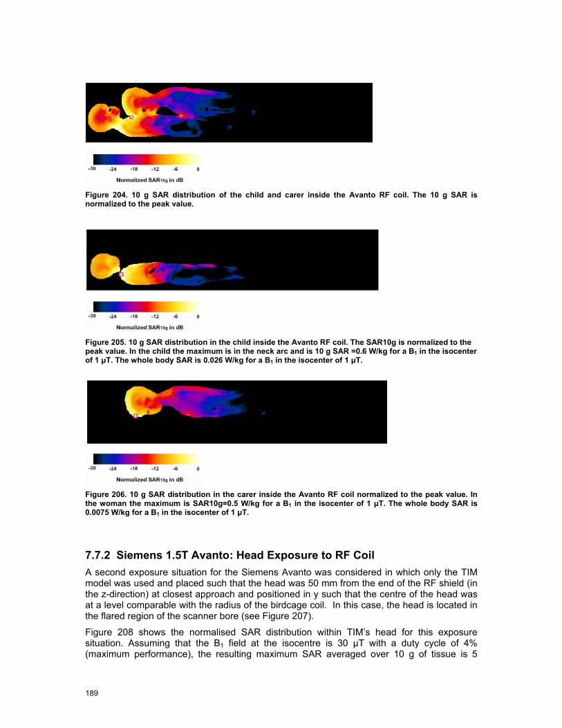
189
Figure 204. 10 g SAR distribution of the child and carer inside the Avanto RF coil. The 10 g SAR is normalized to the peak value.
Figure 205. 10 g SAR distribution in the child inside the Avanto RF coil. The SAR10g is normalized to the peak value. In the child the maximum is in the neck arc and is 10 g SAR =0.6 W/kg for a B1 in the isocenter of 1 µT. The whole body SAR is 0.026 W/kg for a B1 in the isocenter of 1 µT.
Figure 206. 10 g SAR distribution in the carer inside the Avanto RF coil normalized to the peak value. In the woman the maximum is SAR10g=0.5 W/kg for a B1 in the isocenter of 1 µT. The whole body SAR is 0.0075 W/kg for a B1 in the isocenter of 1 µT.
7.7.2 Siemens 1.5T Avanto: Head Exposure to RF Coil A second exposure situation for the Siemens Avanto was considered in which only the TIM model was used and placed such that the head was 50 mm from the end of the RF shield (in the z-direction) at closest approach and positioned in y such that the centre of the head was at a level comparable with the radius of the birdcage coil. In this case, the head is located in the flared region of the scanner bore (see Figure 207).
Figure 208 shows the normalised SAR distribution within TIM’s head for this exposure situation. Assuming that the B1 field at the isocentre is 30 µT with a duty cycle of 4% (maximum performance), the resulting maximum SAR averaged over 10 g of tissue is 5
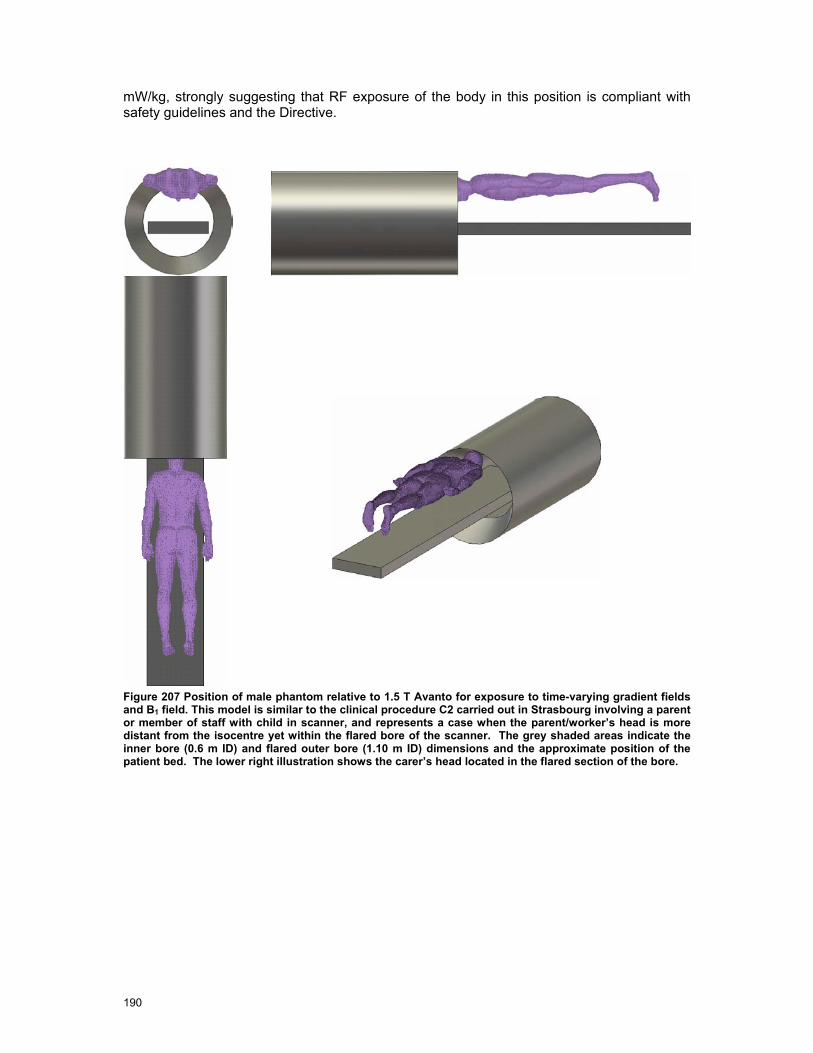
190
mW/kg, strongly suggesting that RF exposure of the body in this position is compliant with safety guidelines and the Directive.
Figure 207 Position of male phantom relative to 1.5 T Avanto for exposure to time-varying gradient fields and B1 field. This model is similar to the clinical procedure C2 carried out in Strasbourg involving a parent or member of staff with child in scanner, and represents a case when the parent/worker’s head is more distant from the isocentre yet within the flared bore of the scanner. The grey shaded areas indicate the inner bore (0.6 m ID) and flared outer bore (1.10 m ID) dimensions and the approximate position of the patient bed. The lower right illustration shows the carer’s head located in the flared section of the bore.

191
Figure 208 SAR10g distribution in the head of TIM model due to Avanto body coil. The body was is positioned relative to the bore of the scanner as shown in Fig 4.22. Here the shortest distance between the head and the end of the RF shield is shown. The sagittal section shown is in the plane x= 0.297 m, the axes indicate the scanner isocentre, and the SAR colour scale is normalised to the peak SAR10g. This is approximately 5 mW/kg when the isocentric B1 was 30 µT and duty cycle is 4 %.
7.7.3 Siemens 1.5 T Avanto: Bystander Exposure In a third exposure situation, the SAR in an adult male model (Duke) standing in a very close position to the scanner was simulated (Figure 209).
Figure 209. Position of the Duke model with respect to the shield of the RF coil.
Figure 210 shows the 10 g SAR distribution on the Duke model. The maximum value occurs in the arm which is closer to the hole of the bore, and has a value of 10 g SAR = 0.875 mW/kg for a B1 in the isocenter of 1 µT. The whole body SAR is 0.057 mW/kg. The results normalized to the measured incident RF field are discussed in Section 7.7.5.
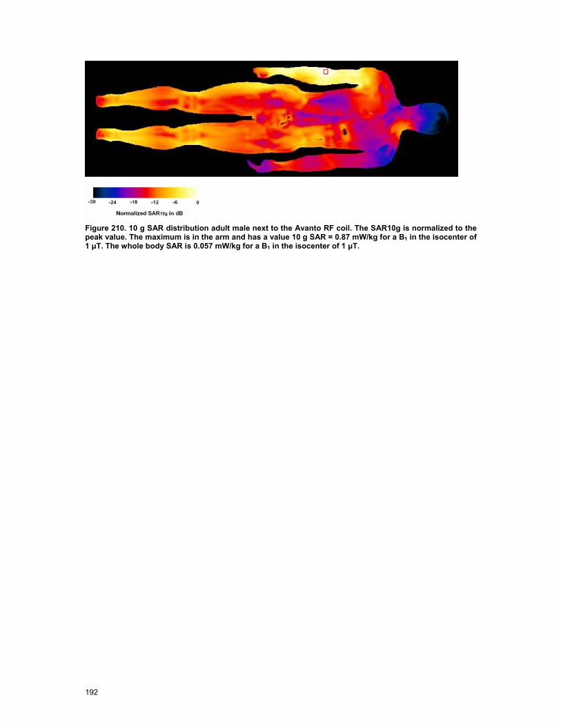
192
Figure 210. 10 g SAR distribution adult male next to the Avanto RF coil. The SAR10g is normalized to the peak value. The maximum is in the arm and has a value 10 g SAR = 0.87 mW/kg for a B1 in the isocenter of 1 µT. The whole body SAR is 0.057 mW/kg for a B1 in the isocenter of 1 µT.

193
7.7.4 Philips 1.0 T Panorama: Radiologist Exposure Figure 211 shows the position assumed in the modeling of the 1.0 T Panorama within a screened enclosure and the position of the male phantom TIM relative to the scanner. This model approximates the exposure of the radiologist performing clip insertion (procedure C2 observed in Cologne). The body was positioned such that the head was in a similar location to the radiologist’s when a patient is present with their right breast at the scanner isocentre. Since it was not possible to articulate the TIM model within the time constraints of the project, the axis of body was assumed to be approximately horizontal and rotated relative to the patient couch by 30 degrees. The distribution of the peak spatial average SAR of the simulation using SEMCAD X is shown in Figure 211. Position of male phantom relative to Panorama 1.0 T, approximating exposure of radiologist performing clip insertion (procedure C2 observed in Cologne). Top: Footprint of Panorama and its position within a screened room 7.1 m x 5.5 m. The height of the room is 2.69 m and the horizontal mid-plane of the scanner was 1.085 m above the floor. The patient couch is to the right (+x direction) of the scanner as shown. The body is positioned horizontally with the longitudinal axis approximately 30 degrees with respect to the patient couch (x-axis) and the head such that the eyes are approximately in the x=0 plane but displaced in +y direction by 0.3 m. This position of the head is similar to that of the radiologist when a patient is present with their right breast at the scanner isocentre. Lower left and right: Views from right to left (x-z plane) (lower left) and from rear to front (y-z plane) (lower right) showing vertical position of head/trunk with respect to the centre of the scanner.The results normalized to the measured incident RF field are discussed in Section 7.7.5.
Figure 211. Position of male phantom relative to Panorama 1.0 T, approximating exposure of radiologist performing clip insertion (procedure C2 observed in Cologne). Top: Footprint of Panorama and its position within a screened room 7.1 m x 5.5 m. The height of the room is 2.69 m and the horizontal mid-
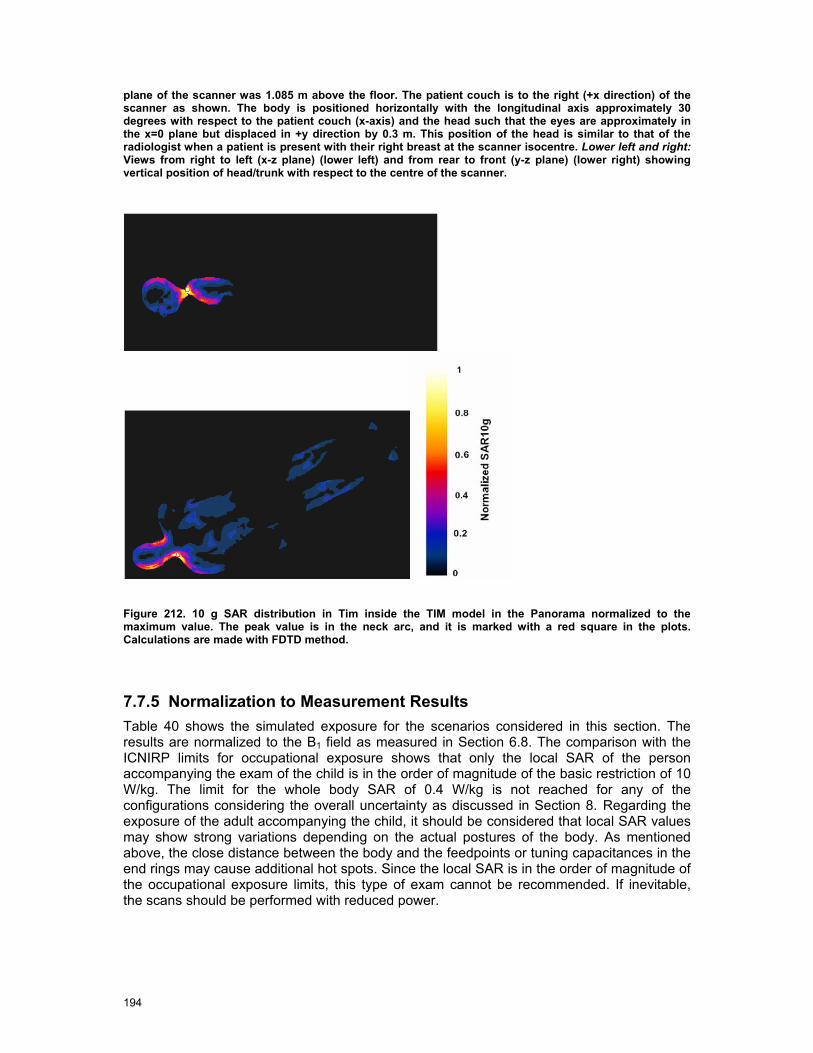
194
plane of the scanner was 1.085 m above the floor. The patient couch is to the right (+x direction) of the scanner as shown. The body is positioned horizontally with the longitudinal axis approximately 30 degrees with respect to the patient couch (x-axis) and the head such that the eyes are approximately in the x=0 plane but displaced in +y direction by 0.3 m. This position of the head is similar to that of the radiologist when a patient is present with their right breast at the scanner isocentre. Lower left and right: Views from right to left (x-z plane) (lower left) and from rear to front (y-z plane) (lower right) showing vertical position of head/trunk with respect to the centre of the scanner.
Figure 212. 10 g SAR distribution in Tim inside the TIM model in the Panorama normalized to the maximum value. The peak value is in the neck arc, and it is marked with a red square in the plots. Calculations are made with FDTD method.
7.7.5 Normalization to Measurement Results Table 40 shows the simulated exposure for the scenarios considered in this section. The results are normalized to the B1 field as measured in Section 6.8. The comparison with the ICNIRP limits for occupational exposure shows that only the local SAR of the person accompanying the exam of the child is in the order of magnitude of the basic restriction of 10 W/kg. The limit for the whole body SAR of 0.4 W/kg is not reached for any of the configurations considering the overall uncertainty as discussed in Section 8. Regarding the exposure of the adult accompanying the child, it should be considered that local SAR values may show strong variations depending on the actual postures of the body. As mentioned above, the close distance between the body and the feedpoints or tuning capacitances in the end rings may cause additional hot spots. Since the local SAR is in the order of magnitude of the occupational exposure limits, this type of exam cannot be recommended. If inevitable, the scans should be performed with reduced power.
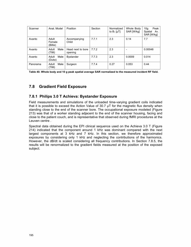
195
Scanner Anat. Model Position Section Normalized
to B1 [µT] Whole Body SAR [W/kg]
10g Peak Spatial Av. SAR [W/kg]
Avanto Adult Female (Billie)
Accompanying Child
7.7.1 2.3 0.14 7.7
Avanto Adult Male (TIM)
Head next to bore opening
7.7.2 2.3 - 0.00048
Avanto Adult Male (Duke)
Bystander 7.7.3 2.3 0.0009 0.014
Panorama Adult Male (TIM)
Surgeon 7.7.4 0.27 0.053 0.44
Table 40. Whole body and 10 g peak spatial average SAR normalized to the measured incident RF field.
7.8 Gradient Field Exposure
7.8.1 Philips 3.0 T Achieva: Bystander Exposure Field measurements and simulations of the unloaded time-varying gradient coils indicated that it is possible to exceed the Action Value of 30.7 µT for the magnetic flux density when standing close to the end of the scanner bore. The occupational exposure modeled (Figure 213) was that of a worker standing adjacent to the end of the scanner housing, facing and close to the patient couch, and is representative that observed during fMRI procedures at the Leuven centre .
Spectral data obtained during the EPI clinical sequence used on the Achieva 3.0 T (Figure 214) indicated that the component around 1 kHz was dominant compared with the next largest components at 3 kHz and 7 kHz. In this section, we therefore approximated exposures by considering only 1 kHz and neglecting the contributions of the harmonics. However, the dB/dt is scaled considering all frequency contributions. In Section 7.8.5, the results will be renormalized to the gradient fields measured at the position of the exposed subject.
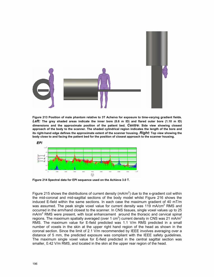
196
Figure 213 Position of male phantom relative to 3T Acheiva for exposure to time-varying gradient fields. Left: The grey shaded areas indicate the inner bore (0.6 m ID) and flared outer bore (1.10 m ID) dimensions and the approximate position of the patient bed. Centre: Side view showing closest approach of the body to the scanner. The shaded cylindrical region indicates the length of the bore and its right-hand edge defines the approximate extent of the scanner housing. Right: Top view showing the body close to and facing the patient bed for the position of closest approach to the scanner housing.
Figure 214 Spectral data for EPI sequence used on the Achieva 3.0 T.
Figure 215 shows the distributions of current density (mA/m2) due to the x-gradient coil within the mid-coronal and mid-sagittal sections of the body model whilst Figure 216 shows the induced E-field within the same sections. In each case the maximum gradient of 40 mT/m was assumed. The peak single voxel value for current density was 119 mA/cm2 RMS and occurred in the arm/hand closest to the scanner. In CNS tissues, single voxel values up to 25 mA/m2 RMS were present, with local enhancement around the thoracic and cervical spinal regions. The maximum spatially averaged (over 1 cm2) current density in CNS was 21 mA/m2 RMS. The maximum value for E-field predicted was 1.1 V/m RMS predicted in a small number of voxels in the skin at the upper right hand region of the head as shown in the coronal section. Since the limit of 2.1 V/m recommended by IEEE involves averaging over a distance of 5 mm, the predicted exposure was compliant with the IEEE safety guidelines. The maximum single voxel value for E-field predicted in the central sagittal section was smaller, 0.42 V/m RMS, and located in the skin at the upper rear region of the head.
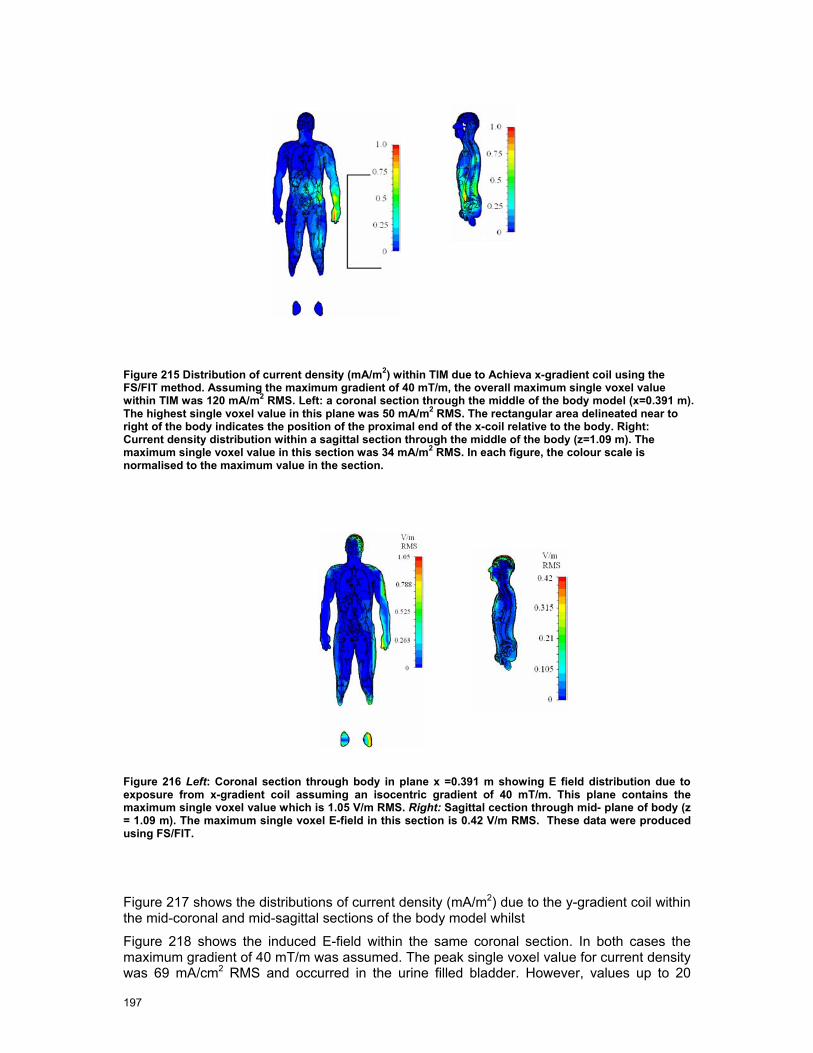
197
Figure 215 Distribution of current density (mA/m2) within TIM due to Achieva x-gradient coil using the FS/FIT method. Assuming the maximum gradient of 40 mT/m, the overall maximum single voxel value within TIM was 120 mA/m2 RMS. Left: a coronal section through the middle of the body model (x=0.391 m). The highest single voxel value in this plane was 50 mA/m2 RMS. The rectangular area delineated near to right of the body indicates the position of the proximal end of the x-coil relative to the body. Right: Current density distribution within a sagittal section through the middle of the body (z=1.09 m). The maximum single voxel value in this section was 34 mA/m2 RMS. In each figure, the colour scale is normalised to the maximum value in the section.
Figure 216 Left: Coronal section through body in plane x =0.391 m showing E field distribution due to exposure from x-gradient coil assuming an isocentric gradient of 40 mT/m. This plane contains the maximum single voxel value which is 1.05 V/m RMS. Right: Sagittal cection through mid- plane of body (z = 1.09 m). The maximum single voxel E-field in this section is 0.42 V/m RMS. These data were produced using FS/FIT.
Figure 217 shows the distributions of current density (mA/m2) due to the y-gradient coil within the mid-coronal and mid-sagittal sections of the body model whilst
Figure 218 shows the induced E-field within the same coronal section. In both cases the maximum gradient of 40 mT/m was assumed. The peak single voxel value for current density was 69 mA/cm2 RMS and occurred in the urine filled bladder. However, values up to 20

198
mA/m2 RMS were also present within the CNS, with local enhancement around the thoracic and cervical spinal regions. The peak spatially averaged (over 1 cm2) RMS value in the central nervous system was 13 mA/m2. The maximum value for E-field predicted is 0.84 V/m RMS predicted in the hand closest to the scanner, suggesting that the predicted exposure is compliant the IEEE safety guidelines.
Figure 217 Distribution of current density (mA/m2) within TIM due to Achieva y-gradient coil using the FS/FIT method. Assuming the maximum gradient of 40 mT/m, the overall maximum single voxel value within TIM was 69 mA/m2 RMS. Left: a coronal section through the middle of the body model (x=0.391 m). The highest single voxel value in this plane was 66 mA/m2. The rectangular area delineated near to right of the body indicates the position of the proximal end of the y-coil relative to the body. Right: Current density distribution within a sagittal section through the middle of the body (z=1.09m). The maximum single voxel value in this section was 44 mA/m2. In each figure, the colour scale is normalised to the maximum value in the section.
Figure 218 Coronal section through body in plane x =0.391 m showing E field distribution due to exposure from y-gradient coil assuming the isocentric gradient is 40 mT/m. This plane contains the maximum single voxel value which is 0.84 V/m RMS. These data were produced using FS/FIT.Figure 219 shows the distributions of current density (mA/m2) due to the z-gradient coil within the mid-coronal and mid-sagittal sections of the body model whilst

199
Figure 220 shows the induced E-field within the same coronal section. The maximum gradient of 40 mT/m was assumed. The peak single voxel value for current density was 20 mA/m2 RMS and occurred in the arm closest to the scanner. In CNS, single voxel values up to 5 mA/m2 were present, with local enhancement around the lumbar, thoracic and cervical spinal regions. The peak spatially averaged (over 1 cm2) RMS value in the central nervous system was 2.7 mA/m2. The maximum value for E-field predicted was 0.32 V/m RMS predicted in the arm closest to the scanner, suggesting that the predicted exposure is compliant the IEEE safety guidelines. Figure 221 shows the induced current densities in the same configurations simulated with the quasistatic solver of SEMCAD X. The differences to the results obtained from FS/FIT are less than 2 dB.
Figure 219 Distribution of current density (mA/m2) within TIM due to Achieva z-gradient coil using the FS/FIT method. Assuming the maximum gradient of 40 mT/m, the overall maximum single voxel value within TIM was 20 mA/m2 RMS. Left: a coronal section through the middle of the body model (x=0.391 m). The highest single voxel value in this plane was 8.5 mA/m2 RMS. The rectangular area delineated near to right of the body indicates the position of the proximal end of the y-coil relative to the body. Right: Current density distribution within a sagittal section through the middle of the body (z=1.09 m). The maximum single voxel value in this section was 3.5 mA/m2 RMS. In each figure, the colour scale is normalised to the maximum value in the section.

200
Figure 220 Coronal section through body in plane x =0.391 m showing E field distribution due to exposure from z-gradient coil assuming the isocentric gradient is 40 mT/m. This plane contains the maximum single voxel value which is 0.32 V/m RMS. These data were produced using FS/FIT.
0
-20
-40
-60
-80
-100
Current Density [dB]
x-gradient coil y-gradient coil z-gradient coil Figure 221 Current densities in the center planes of the TIM model at 40mT/m at 1 kHz. 0 dB correspond to 2 A/m2
RMS. The maximum single voxel values are 140 mA/m2RMS (x-gradient coil) 100 mA/m2
RMS (y-gradient coil) and 24 mA/m2
RMS (z-gradient coil).
7.8.2 Siemens 1.5T Avanto: Head Exposure to Gradient Coil The exposure to the current densities induced by z-gradient coil of the 1.5 T Avanto has been evaluated for the configuration discussed in Section 7.7.2. Figure 222and
Figure 223 show current density and electric field distributions within the body due to exposure from the Avanto z-gradient coil, assuming the maximum isocentric gradient of 45 mT/m. Fig 4.26 shows that the maximum current density occurred in the head. Single voxel values up to 53 mA/m2 were predicted. The maximum spatially averaged (over 1 cm2) RMS current density in CNS was also 53 mA/m2. In fig 4.27, the maximum E-field in the mid-coronal section of the body occurred in the head and was 0.32 V/m. This hot spot was also seen in the mid-sagittal section

201
Figure 222 Distribution of current density (mA/m2) within the body model as positioned in Fig 4.24 due to Avanto z-gradient coil. Data generated using FS/FIT and for the maximum gradient of 45 mT/m. Left: within a coronal plane (y=0.33 m) Right within a sagittal plane (x=0.241 m) These planes contained the highest single voxel value of current density (58.3 mA/m2 RMS). The areas delineated near to the head indicate the position of the proximal end of the z-coil relative to the body. The colour scale is normalised to the maximum in plane single voxel value.
Figure 223 Left: Coronal section through body in plane y=0.33 m showing E field distribution due to exposure from z-gradient coil assuming the isocentric gradient is 45 mT/m. This plane contains the maximum single voxel value which is 0.32 V/m. Right: Section through mid-sagittal plane of body (x =0.8 m). The maximum E-field in this section is 0.28 V/m. These data were produced using FS/FIT.

202
7.8.3 Siemens 1.5T Avanto: Exposure of Carer to Gradient Coil The current density induced in the accompanying carer by the x-, y- and z-gradient coils of the 1.5 T Avanto has been evaluated for the configuration discussed in Section 7.7.1. Figure 224 shows the distribution of the current densities both in the carer and in the patient. Normalized to the measured dB/dt of 0.7 T/s (x- and y-coils) and 2.0 T/s (z-coil), a maximum exposure of 0.91 A/m² occur in the carer (see Section 7.8.5 for details) exposed to the y-gradient coil because of the close distance to the current maxima. Moreover, peak current densities of >1.2 A/m² have been observed in the patient. These strongly depend on gaps between the two bodies and loops formed by them. In conclusion, application of this scanning procedure is questionable because it leads to a strongly enhanced exposure of the carer.
Figure 224 Normalized current densities induced in the carere and the patient exposed to the gradient coils of the Siemens 1.5 T Avanto.
7.8.4 Philips 1T Panorama: Radiologist Exposure Figure 225 shows the predicted (using FS/FIT) H-field produced by the Panorama vertical gradient coil showing region in which H > 24 A/m, the action value when 0.82 kHz <f < 65 kHz, for the case of an isocentric gradient value of 26 mT/m. The boundary between red and yellow shading corresponds closely to the footprint of the scanner (see Figure 211). Clearly, the position of the body considered here is such that there is an exposure to H field greater than the action value.
Figure 226 shows the current density distribution within the body section in plane at x=0.261 m, a plane that contained the maximum single voxel value (1.2 A/m2 RMS) in CNS tissue, due to exposure to the z-gradient fields assuming the maximum gradient of 26 mT/m. Data
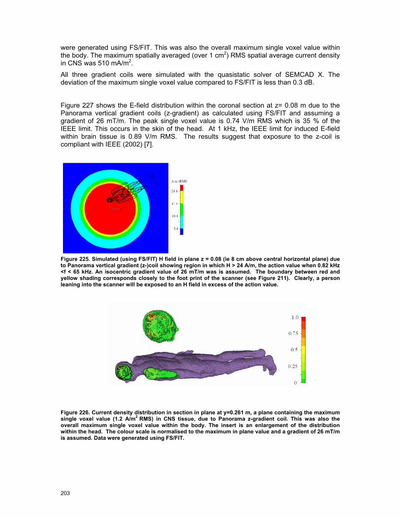
203
were generated using FS/FIT. This was also the overall maximum single voxel value within the body. The maximum spatially averaged (over 1 cm2) RMS spatial average current density in CNS was 510 mA/m2.
All three gradient coils were simulated with the quasistatic solver of SEMCAD X. The deviation of the maximum single voxel value compared to FS/FIT is less than 0.3 dB.
Figure 227 shows the E-field distribution within the coronal section at z= 0.08 m due to the Panorama vertical gradient coils (z-gradient) as calculated using FS/FIT and assuming a gradient of 26 mT/m. The peak single voxel value is 0.74 V/m RMS which is 35 % of the IEEE limit. This occurs in the skin of the head. At 1 kHz, the IEEE limit for induced E-field within brain tissue is 0.89 V/m RMS. The results suggest that exposure to the z-coil is compliant with IEEE (2002) [7].
Figure 225. Simulated (using FS/FIT) H field in plane z = 0.08 (ie 8 cm above central horizontal plane) due to Panorama vertical gradient (z-)coil showing region in which H > 24 A/m, the action value when 0.82 kHz <f < 65 kHz. An isocentric gradient value of 26 mT/m was is assumed. The boundary between red and yellow shading corresponds closely to the foot print of the scanner (see Figure 211). Clearly, a person leaning into the scanner will be exposed to an H field in excess of the action value.
Figure 226. Current density distribution in section in plane at y=0.261 m, a plane containing the maximum single voxel value (1.2 A/m2 RMS) in CNS tissue, due to Panorama z-gradient coil. This was also the overall maximum single voxel value within the body. The insert is an enlargement of the distribution within the head. The colour scale is normalised to the maximum in plane value and a gradient of 26 mT/m is assumed. Data were generated using FS/FIT.
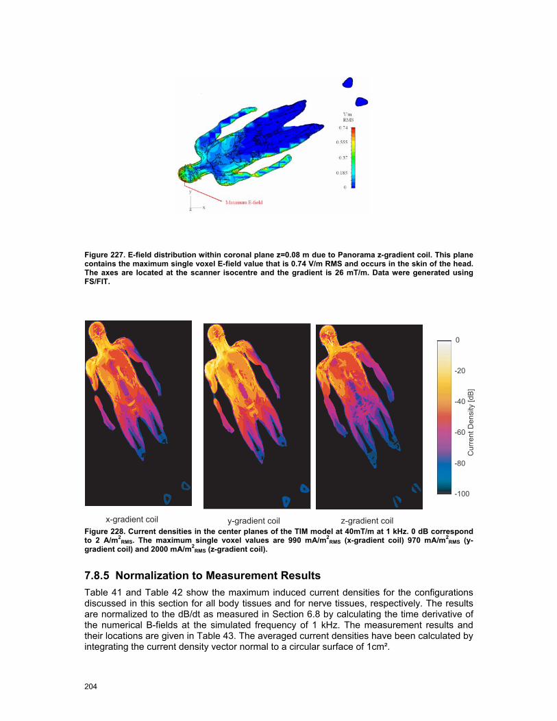
204
Figure 227. E-field distribution within coronal plane z=0.08 m due to Panorama z-gradient coil. This plane contains the maximum single voxel E-field value that is 0.74 V/m RMS and occurs in the skin of the head. The axes are located at the scanner isocentre and the gradient is 26 mT/m. Data were generated using FS/FIT.
0
-20
-40
-60
-80
-100
Current Density [dB]
y-gradient coil z-gradient coilx-gradient coilFigure 228. Current densities in the center planes of the TIM model at 40mT/m at 1 kHz. 0 dB correspond to 2 A/m2
RMS. The maximum single voxel values are 990 mA/m2RMS (x-gradient coil) 970 mA/m2
RMS (y-gradient coil) and 2000 mA/m2
RMS (z-gradient coil).
7.8.5 Normalization to Measurement Results Table 41 and Table 42 show the maximum induced current densities for the configurations discussed in this section for all body tissues and for nerve tissues, respectively. The results are normalized to the dB/dt as measured in Section 6.8 by calculating the time derivative of the numerical B-fields at the simulated frequency of 1 kHz. The measurement results and their locations are given in Table 43. The averaged current densities have been calculated by integrating the current density vector normal to a circular surface of 1cm².
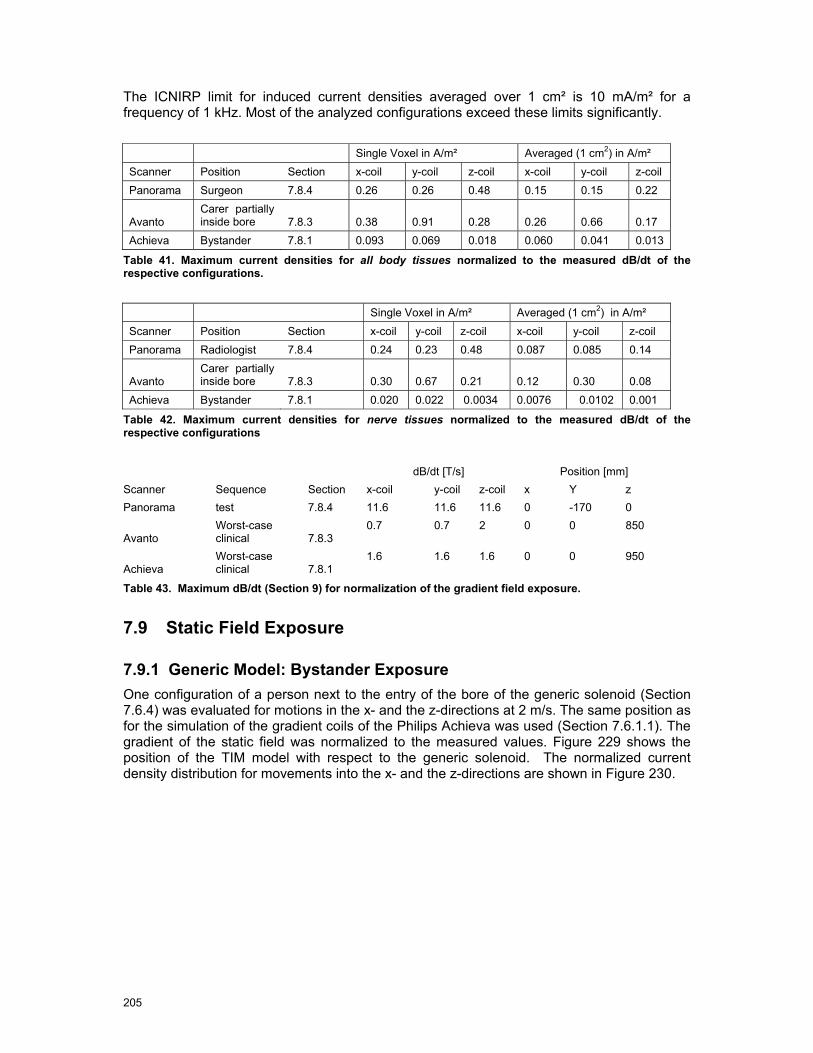
205
The ICNIRP limit for induced current densities averaged over 1 cm² is 10 mA/m² for a frequency of 1 kHz. Most of the analyzed configurations exceed these limits significantly.
Single Voxel in A/m² Averaged (1 cm2) in A/m² Scanner Position Section x-coil y-coil z-coil x-coil y-coil z-coil Panorama Surgeon 7.8.4 0.26 0.26 0.48 0.15 0.15 0.22
Avanto Carer partially inside bore 7.8.3 0.38 0.91 0.28 0.26 0.66 0.17
Achieva Bystander 7.8.1 0.093 0.069 0.018 0.060 0.041 0.013
Table 41. Maximum current densities for all body tissues normalized to the measured dB/dt of the respective configurations.
Single Voxel in A/m² Averaged (1 cm2) in A/m² Scanner Position Section x-coil y-coil z-coil x-coil y-coil z-coil Panorama Radiologist 7.8.4 0.24 0.23 0.48 0.087 0.085 0.14
Avanto Carer partially inside bore 7.8.3 0.30 0.67 0.21 0.12 0.30 0.08
Achieva Bystander 7.8.1 0.020 0.022 0.0034 0.0076 0.0102 0.001
Table 42. Maximum current densities for nerve tissues normalized to the measured dB/dt of the respective configurations
dB/dt [T/s] Position [mm] Scanner Sequence Section x-coil y-coil z-coil x Y z Panorama test 7.8.4 11.6 11.6 11.6 0 -170 0
Avanto Worst-case clinical 7.8.3
0.7 0.7 2 0 0 850
Achieva Worst-case clinical 7.8.1
1.6 1.6 1.6 0 0 950
Table 43. Maximum dB/dt (Section 9) for normalization of the gradient field exposure.
7.9 Static Field Exposure
7.9.1 Generic Model: Bystander Exposure One configuration of a person next to the entry of the bore of the generic solenoid (Section 7.6.4) was evaluated for motions in the x- and the z-directions at 2 m/s. The same position as for the simulation of the gradient coils of the Philips Achieva was used (Section 7.6.1.1). The gradient of the static field was normalized to the measured values. Figure 229 shows the position of the TIM model with respect to the generic solenoid. The normalized current density distribution for movements into the x- and the z-directions are shown in Figure 230.
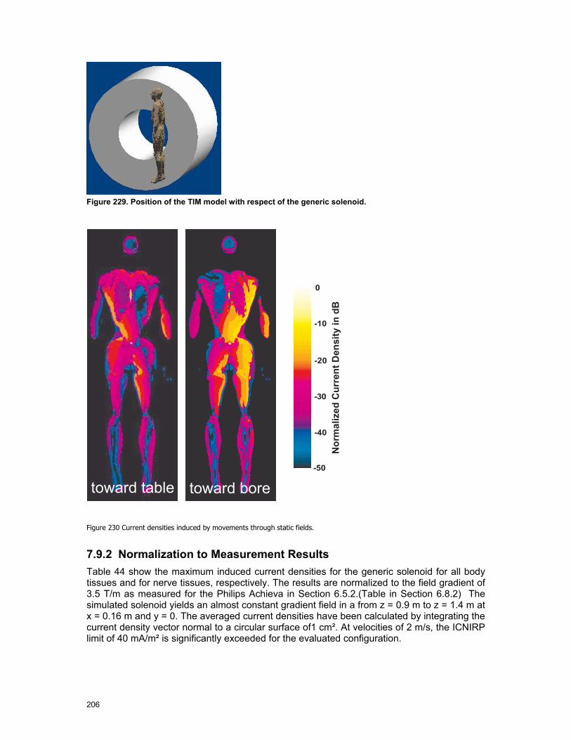
206
Figure 229. Position of the TIM model with respect of the generic solenoid.
Figure 230 Current densities induced by movements through static fields.
7.9.2 Normalization to Measurement Results Table 44 show the maximum induced current densities for the generic solenoid for all body tissues and for nerve tissues, respectively. The results are normalized to the field gradient of 3.5 T/m as measured for the Philips Achieva in Section 6.5.2.(Table in Section 6.8.2) The simulated solenoid yields an almost constant gradient field in a from z = 0.9 m to z = 1.4 m at x = 0.16 m and y = 0. The averaged current densities have been calculated by integrating the current density vector normal to a circular surface of1 cm². At velocities of 2 m/s, the ICNIRP limit of 40 mA/m² is significantly exceeded for the evaluated configuration.

207
All Tissues Nerve Tissues Single Voxel in A/m² Averaged in A/m² Single Voxel in A/m² Averaged in A/m² x-direction
z-direction
x-direction
z-direction
x-direction
z-direction
x-direction
z-direction
0.23 0.45 0.16 0.33 0.095 0.18 0.046 0.094
Table 44. Current densities induced for movement through static fields at 2 m/s normalized to the field gradient of 3.5 T/m of the Philips Achieva in front of the bore.
7.10 Summary and Requirements
The comparison of the dosimetric quantities assessed in this section with basic restrictions for the exposure of the human body to electromagnetic fields show by which extent occupational exposure during typical situations can exceed safety limits. Violations mainly occur for low frequency and static magnetic fields. Only in one particular case, adult accompanying child inside the scanner bore, the peak spatial average SAR was in the order of magnitude of the exposure limits.
Nevertheless, the uncertainties of the computational results as discussed in Section 8 are significant. In many instances, they are due to strong simplifications of the numerical models of the MRI scanners. These were inevitable because (a) manufacturers were not willing to disclose complete descriptions of their coil and magnet designs and (b) the data and models provided by one manufacturer had been developed primarily to study the fields outside the bore rather than the fields inside the bore, as these are of interest in the case of most occupational exposures. Effects such as detuning of the RF coils, interaction of gradient and static fields with magnetic materials or shimming coils, etc., could not be taken into account in the simulations carried out here. On the other hand, the numerical tools and anatomical models are available to the manufacturers, and analyses of the occupational safety can be carried out by them with significantly reduced uncertainty of the scanner models.
In addition to the improved numerical models of the MR scanners, requirements to reduce the uncertainty and to better assess the variability of the exposure are:
• Advanced CAD models of the human body including, e. g., obese and pregnant models
• Tools to articulate the limbs of the models for a more realistic representation of postures during typical occupational scenarios
• Advanced numerical methods to analyze the induced temperature distribution in the body considering blood flow and thermoregulatory effects

8 Uncertainty Assessment
8.1 Introduction
The aims of the following uncertainty evaluations are the assessments of the offset and uncertainty with respect to worst-case incident exposure and induced fields for occupational personnel operating, assisting and cleaning MRI medical facilities. These include the determination of
• the measurement uncertainty,
• the extrapolation uncertainty and
• the translation of these incident exposure situations to induced current and SAR that enables the comparison with the basic restrictions of the safety guidelines.
All these values as well as the combined uncertainty are given in the following Tables. The uncertainty values may appear surprisingly large for non-experts. However, MRIs constitute a hostile environment for measurements with limited access. Furthermore, there was neither sufficient time nor resources to develop equipment optimised for these tasks. The extrapolation to other scanners is difficult and therefore the offset and the uncertainties have been conservatively estimated. The uncertainties of the extrapolation from the few cases (anatomies & postures) for the induced fields were estimated based on knowledge from similar studies conducted by the same authors.
Please note that the extrapolation to worst-case is treated the same way, i.e., with an offset and uncertainty term.
8.2 Concept of Uncertainty Assessment
Methodologies for determining the uncertainties of experiments involving quantities that cannot be assessed by statistical means were developed for electromagnetic compatibilities, as described in, for example, Taylor and Kuyatt [1994] [94] or ISO/IEC “Guide to the Expression of Uncertainty in Measurement”. It has also been applied in dosimetry [Kuster Error! Reference source not found.]. The methods are based on splitting the total uncertainty into various uncertainty sources that are independent or with limited interdependencies, determining the uncertainty from assumed statistical models, and calculations of the total uncertainty as the root-sum-square (RSS) value.
∑=
⋅=m
iiic ucu
1
22
The standard uncertainty ui evaluation will mainly based on Type B, i.e., ui comes from the upper +a and lower −a limits of the quantity in question, depending on the distribution law defining 2)( −+ −= aaa , then:
Rectangular law: 3aui =
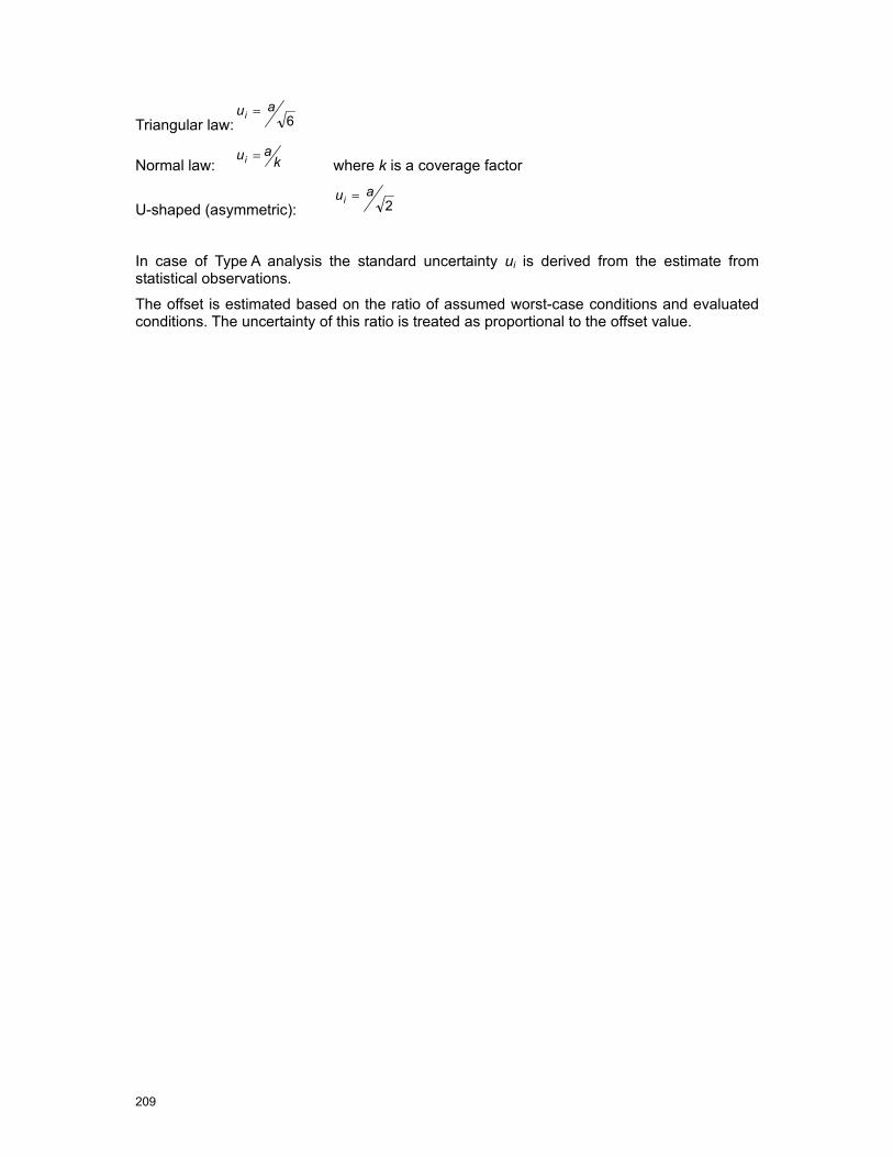
209
Triangular law: 6aui =
Normal law: kaui =
where k is a coverage factor
U-shaped (asymmetric): 2aui =
In case of Type A analysis the standard uncertainty ui is derived from the estimate from statistical observations.
The offset is estimated based on the ratio of assumed worst-case conditions and evaluated conditions. The uncertainty of this ratio is treated as proportional to the offset value.

210
8.3 Offset and Uncertainty of Static Magnetic Field Evaluation
Uncertainty Component Tolerance of Parameter
Offset in dB
Tolerance for U_meas in dB
Probality Distri.
Div
isor
Wei
ght
Unc. in dB
Measurement System
- Probe Calibration 0.0 0.17 normal 1 1 0.2 Note 1
- Spherical Isotropy 0.0 0.20 rect. 1.73 1 0.1 Note 1
- Sensor Displacement 0.0 0.00 rect. 1.73 1 0.0 Note 2
- Linearity 0.0 0.20 rect. 1.73 1 0.1 Note 1
- System Detection Limits 0.0 0.04 rect. 1.73 1 0.0 Note 1
- Readout Electronics 0.0 0.01 normal 1 1 0.0 Note 1
- Response Time 0.0 0.00 rect. 1.73 1 0.0 Note 3
- Integration Time 0.0 0.11 rect. 1.73 1 0.1 Note 3
- Ambient Conditions 0.0 0.00 rect. 1.73 1 0.0 Note 4
- Probe Position 10mm 0.0 0.17 rect. 1.73 1 0.1 Note 2
Combined Meas. Uncertainty 0.0 0.3
Extrapolation Worst-Case
- all scanners 0.0 1.00 rect. 1.73 1 0.6 Note 5
Extrapolation Uncertainty 0.0 0.6
Total Uncertainty SUM 0.0 RSS 0.6
Coverage Factor for 95% 1 k 2
Offset / Expanded Uncertainty 0.0 1.3
Table 45: Offset & Uncertainty Budget for the Static Magnetic Field Evaluation.
Note 1 Assessment of the uncertainty by evaluation inside the bore
Note 2 In comparison with probe positioning uncertainty, this term can be neglected; The gradient is larger outside except for the 7T
Note 3 The probe was manual placed and the integration time was set to 0.4s.
Note 4 The fields are greatly above any ambient field levels.
Note 5 Estimated based on good engineering considerations

211
8.4 Offset and Uncertainty of Gradient Field Evaluation
Uncertainty Component Tolerance of Parameter
Offset in dB
Tolerance for U_meas in dB
Probality Distri.
Div
isor
Wei
ght
Unc. in dB
Measurement System
- Probe Calibration for MR gradients 0.0 0.80 normal 1.73 1 0.5 Note 1
- Spherical Isotropy 0.0 0.20 rect. 1.73 1 0.1 Note 2
- Sensor Displacement 0.0 0.00 rect. 1.73 1 0.0 Note 3
- Linearity 0.0 0.50 rect. 1.73 1 0.3 Note 2
- Frequency Response 0.0 0.80 rect. 1.73 1 0.5 Note 2
- System Detection Limits 0.0 0.10 rect. 1.73 1 0.1 Note 2
- Readout Electronics 0.0 0.10 rect 1.73 1 0.1 Note 2
- Movements in Static Fields 0.0 0.20 rect. 1.73 1 0.1 Note 4
- Ambient Conditions 0.0 0.00 rect. 1.73 1 0.0 Note 3
- Spatial Averaging 0.0 1.00 rect. 1.73 1 0.6 Note 3
- Probe Position 10 mm 0.0 0.45 rect. 1.73 1 0.3 Note 3
Combined Meas. Uncertainty 0.0 1.0
Extrapolation to Worst-Case
- w-c sequence / test sequence 0.0 3.00 rect. 1.73 1 1.7 Note 5
- all scanners (same B1&application) 2.0 1.00 rect. 1.73 1 0.6 Note 6
Combined Extrapolation Uncertainty 2.0 1.8
Total Combined Uncertainty SUM 2.0 RSS 2.1
Coverage Factor for 95% 1 2
Offset / Expanded Uncertainty (k=2) 2.0 4.1
Table 46.Offset & Uncertainty Budget for the Incident Gradient Magnetic Field Evaluation
Note 1 Assessment of the uncertainty by evaluation inside the bore (Narda specified 0.4dB)
Note 2 Evaluated in [B-Field Exposure from Inducting Cooking Appliances, 2006]
Note 3 Based on worst-case spatial change of gradients (similar for inside and outside the bore)
Note 4 Largely removed during evaluations
Note 5 Extrapolated in Chapter 6.8 from test sequence to worst-case clinical sequence used in interventional MRI. Uncertainty is estimated as the sequences were only recordered for a finite time (5s)
Note 6 Estimated based on good engineering considerations

212
8.5 Offset & Uncertainty of Incident RF H-Field Evaluation
Uncertainty Component Tolerance of Paramter
Offset in dB
Tolerance for U_meas in dB
Probality Distri.
Div
isor
Wei
ght Unc. in dB
Measurement System
- Probe Calibration CW 0.0 0.22 normal 1 1 0.2 Note 1
- Spherical Isotropy 0.0 0.20 rect. 1.73 1 0.1 Note 1
- Sensor Displacement 0.0 0.00 rect. 1.73 1 0.0 Note 2
- Linearity 0.0 0.20 rect. 1.73 1 0.1 Note 1
- Modulation 0.0 0.80 rect. 1.73 1 0.5 Note 3
- System Detection Limits 0.0 0.04 rect. 1.73 1 0.0 Note 1
- Readout Electronics 0.0 0.01 normal 1 1 0.0 Note 1
- Response Time 0.0 0.03 rect. 1.73 1 0.0 Note 4
- Integration Time 0.0 0.11 rect. 1.73 1 0.1 Note 4
- RF Ambient Conditions 0.0 0.00 rect. 1.73 1 0.0 Note 5
- RF Reflections 0.0 0.30 rect. 1.73 1 0.2 Note 5
- Probe Position 10mm 0.0 0.40 rect. 1.73 1 0.2 Note 2
Combined Meas. Uncertainty 0.0 0.6
c
Extrapolation to Worst-Case
- w-c sequence / test sequence 0.0 1.00 rect. 1.73 1 0.6 Note 6
- all scanners (same B1&application) 3.0 1.50 rect. 1.73 1 0.9 Note 7
Combined Extrapolation Uncertainty 3.0 1.0
Total Combined Uncertainty SUM 3.0 RSS 1.2
Coverage Factor for 95% 1 k 2
Offset / Expanded Uncertainty 3.0 2.4
Table 47. Offset & Uncertainty Budget for the Incident RF Magnetic Field Evaluation (outside bore).
Note 1 Axial isotropy 0.2 dB according to calibration sheet
Note 2 In comparison with probe positioning uncertainty, this term can be neglected (in the bore the probe positioning uncertainty is larger 30mm and estimated 3 dB)
Note 3 The calibration house contracted (speag) did not have availalble stadardised modulation response calibrations. Therefore the modulation compensation was conducted in house
Note 4 The probe was manual placed and the integration time was set to 1 s.
Note 5 Since the MRI equipment is placed in a well screened room, the ambient field can be neglected with device both for E- and H-field; Reflections caused by the wall and operators
Note 6 For Philips the ratio is 1.4 and for Siemens it is 4.5 (already considered in Sections 6.8.2-6.8.3)
Note 7 Estimated based on good engineering considerations
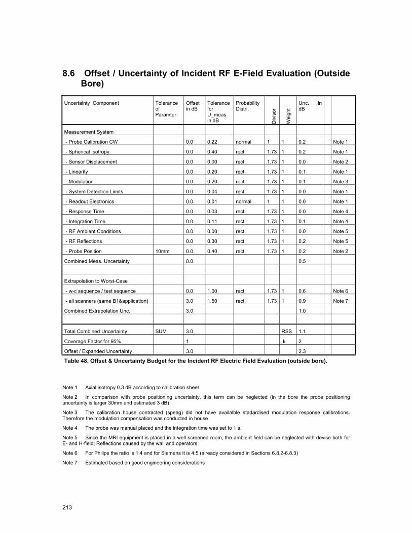
213
8.6 Offset / Uncertainty of Incident RF E-Field Evaluation (Outside Bore)
Uncertainty Component Tolerance of Paramter
Offset in dB
Tolerance for U_meas in dB
Probability Distri.
Div
isor
Wei
ght
Unc. in dB
Measurement System
- Probe Calibration CW 0.0 0.22 normal 1 1 0.2 Note 1
- Spherical Isotropy 0.0 0.40 rect. 1.73 1 0.2 Note 1
- Sensor Displacement 0.0 0.00 rect. 1.73 1 0.0 Note 2
- Linearity 0.0 0.20 rect. 1.73 1 0.1 Note 1
- Modulation 0.0 0.20 rect. 1.73 1 0.1 Note 3
- System Detection Limits 0.0 0.04 rect. 1.73 1 0.0 Note 1
- Readout Electronics 0.0 0.01 normal 1 1 0.0 Note 1
- Response Time 0.0 0.03 rect. 1.73 1 0.0 Note 4
- Integration Time 0.0 0.11 rect. 1.73 1 0.1 Note 4
- RF Ambient Conditions 0.0 0.00 rect. 1.73 1 0.0 Note 5
- RF Reflections 0.0 0.30 rect. 1.73 1 0.2 Note 5
- Probe Position 10mm 0.0 0.40 rect. 1.73 1 0.2 Note 2
Combined Meas. Uncertainty 0.0 0.5
Extrapolation to Worst-Case
- w-c sequence / test sequence 0.0 1.00 rect. 1.73 1 0.6 Note 6
- all scanners (same B1&application) 3.0 1.50 rect. 1.73 1 0.9 Note 7
Combined Extrapolation Unc. 3.0 1.0
Total Combined Uncertainty SUM 3.0 RSS 1.1
Coverage Factor for 95% 1 k 2
Offset / Expanded Uncertainty 3.0 2.3
Table 48. Offset & Uncertainty Budget for the Incident RF Electric Field Evaluation (outside bore).
Note 1 Axial isotropy 0.3 dB according to calibration sheet
Note 2 In comparison with probe positioning uncertainty, this term can be neglected (in the bore the probe positioning uncertainty is larger 30mm and estimated 3 dB)
Note 3 The calibration house contracted (speag) did not have availalble stadardised modulation response calibrations. Therefore the modulation compensation was conducted in house
Note 4 The probe was manual placed and the integration time was set to 1 s.
Note 5 Since the MRI equipment is placed in a well screened room, the ambient field can be neglected with device both for E- and H-field; Reflections caused by the wall and operators
Note 6 For Philips the ratio is 1.4 and for Siemens it is 4.5 (already considered in Sections 6.8.2-6.8.3)
Note 7 Estimated based on good engineering considerations

214
8.7 Offset and Uncertainty of Peak Spatial SAR Values
Uncertainty Component Tolerance
of Parameter
Offset in dB
Tolerance for U_meas in dB
Probability Distribution
Div
isor
Wei
ght
Unc. in dB
Simulation Uncertainty
- Discretization 0.0 0.29 rect. 1.73 1 0.2 Note 1
- ABC 0.0 0.21 rect. 1.73 1 0.1 Note 2
- Power Budget 0.0 0.09 rect. 1.73 1 0.0 Note 2
- Deviation from Steady-State 0.0 0.50 rect. 1.73 1 0.3 Note 2
- Peak Spatial SAR 0.0 0.50 rect. 1.73 1 0.3 Note 3
- MRI device modeling 0.0 3.00 rect. 1.73 1 1.7 Note 5
- Position in Defined Position 0mm 0.0 0.00 rect. 1.73 1 0.0 Note 4
Combined Simulation Uncertainty 0.0 1.8
Extrapolation to Worst-Case
- Incident Field Normalization 3.0 1.14 normal 1 1 1.1 Note 6
- Anatomy 2.0 1.00 rect. 1.73 1 0.6 Note 7
- Posture 2.0 1.00 rect. 1.73 1 0.6 Note 7
- Location 1.0 0.50 rect. 1.73 2 0.6 Note 7
Combined Induced field Uncertainty 8.0 1.5
Total Combined Uncertainty Sum 8.0 RSS 2.3
Coverage Factor for 95% 1 2
Offset / Expanded Uncertainty (k=2) 8.0 4.7
Table 49. Offset & Uncertaitny Budget for the Induced Peak Spatial SAR Field (outside)
Note 1 Based on the peak spatial SAR evaluation of child in a 1.5 T birdcage with resolution for 3 and 1.5 mm (negligible for whole body SAR)
Note 2 Based on generic evaluations
Note 3 Peak spatial SAR was not rotated to find worst-case orientation; uncertainty was only estimated
Note 4 Assumed to be 0 mm since the field are scaled to the measurements
Note 5 The MRI models received from the manufacturers were insufficient to obtain accurate incident field distributions; Strength is normalised to measurements
Note 6 Uncertainty and offset as determined from measurement (see Table 47 and Table 48)
Note 7 Estimated on good engineering considerations.
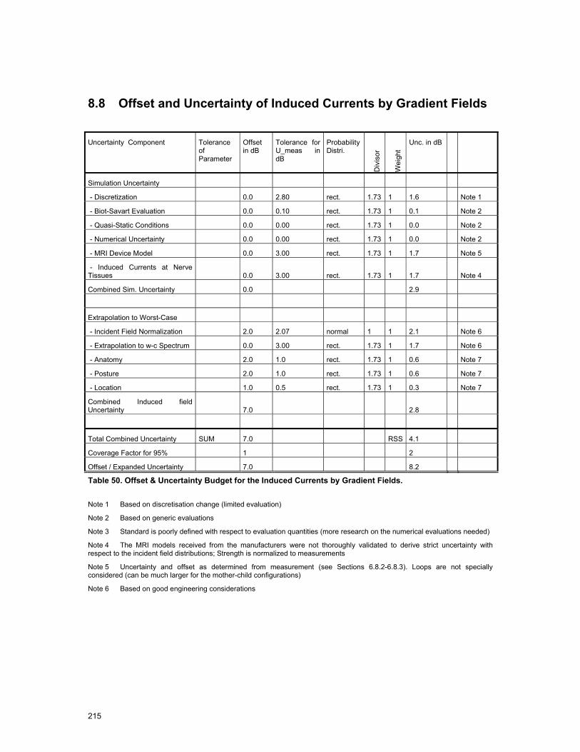
215
8.8 Offset and Uncertainty of Induced Currents by Gradient Fields
Uncertainty Component Tolerance
of Parameter
Offset in dB
Tolerance for U_meas in dB
Probability Distri.
Div
isor
Wei
ght
Unc. in dB
Simulation Uncertainty
- Discretization 0.0 2.80 rect. 1.73 1 1.6 Note 1
- Biot-Savart Evaluation 0.0 0.10 rect. 1.73 1 0.1 Note 2
- Quasi-Static Conditions 0.0 0.00 rect. 1.73 1 0.0 Note 2
- Numerical Uncertainty 0.0 0.00 rect. 1.73 1 0.0 Note 2
- MRI Device Model 0.0 3.00 rect. 1.73 1 1.7 Note 5
- Induced Currents at Nerve Tissues 0.0 3.00 rect. 1.73 1 1.7 Note 4
Combined Sim. Uncertainty 0.0 2.9
Extrapolation to Worst-Case
- Incident Field Normalization 2.0 2.07 normal 1 1 2.1 Note 6
- Extrapolation to w-c Spectrum 0.0 3.00 rect. 1.73 1 1.7 Note 6
- Anatomy 2.0 1.0 rect. 1.73 1 0.6 Note 7
- Posture 2.0 1.0 rect. 1.73 1 0.6 Note 7
- Location 1.0 0.5 rect. 1.73 1 0.3 Note 7
Combined Induced field Uncertainty 7.0 2.8
Total Combined Uncertainty SUM 7.0 RSS 4.1
Coverage Factor for 95% 1 2
Offset / Expanded Uncertainty 7.0 8.2
Table 50. Offset & Uncertainty Budget for the Induced Currents by Gradient Fields.
Note 1 Based on discretisation change (limited evaluation)
Note 2 Based on generic evaluations
Note 3 Standard is poorly defined with respect to evaluation quantities (more research on the numerical evaluations needed)
Note 4 The MRI models received from the manufacturers were not thoroughly validated to derive strict uncertainty with respect to the incident field distributions; Strength is normalized to measurements
Note 5 Uncertainty and offset as determined from measurement (see Sections 6.8.2-6.8.3). Loops are not specially considered (can be much larger for the mother-child configurations)
Note 6 Based on good engineering considerations
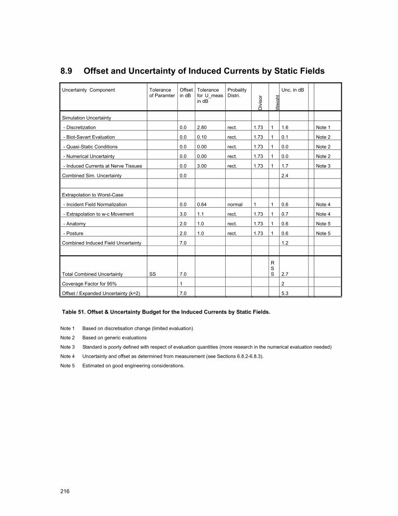
216
8.9 Offset and Uncertainty of Induced Currents by Static Fields
Uncertainty Component Tolerance of Paramter
Offset in dB
Tolerance for U_meas in dB
Probality Distri.
Div
isor
Wei
ght
Unc. in dB
Simulation Uncertainty
- Discretization 0.0 2.80 rect. 1.73 1 1.6 Note 1
- Biot-Savart Evaluation 0.0 0.10 rect. 1.73 1 0.1 Note 2
- Quasi-Static Conditions 0.0 0.00 rect. 1.73 1 0.0 Note 2
- Numerical Uncertainty 0.0 0.00 rect. 1.73 1 0.0 Note 2
- Induced Currents at Nerve Tissues 0.0 3.00 rect. 1.73 1 1.7 Note 3
Combined Sim. Uncertainty 0.0 2.4
Extrapolation to Worst-Case
- Incident Field Normalization 0.0 0.64 normal 1 1 0.6 Note 4
- Extrapolation to w-c Movement 3.0 1.1 rect. 1.73 1 0.7 Note 4
- Anatomy 2.0 1.0 rect. 1.73 1 0.6 Note 5
- Posture 2.0 1.0 rect. 1.73 1 0.6 Note 5
Combined Induced Field Uncertainty 7.0 1.2
Total Combined Uncertainty SS 7.0
RSS 2.7
Coverage Factor for 95% 1 2
Offset / Expanded Uncertainty (k=2) 7.0 5.3
Table 51. Offset & Uncertainty Budget for the Induced Currents by Static Fields.
Note 1 Based on discretisation change (limited evaluation)
Note 2 Based on generic evaluations
Note 3 Standard is poorly defined with respect of evaluation quantities (more research in the numerical evaluation needed)
Note 4 Uncertainty and offset as determined from measurement (see Sections 6.8.2-6.8.3).
Note 5 Estimated on good engineering considerations.

218
9 Conclusions
9.1 Overview
Magnetic Resonance Imaging (MRI) is a rapidly developing non-invasive diagnostic technology that provides an unmatched view inside the human body without applying ionizing radiation. Improved image quality and novel applications, however, generally require higher electromagnetic field (EMF) strengths and faster image acquisitions, both of which result in an increase in the EMF exposure of patients and workers. It has been over the past 30 years that safety standards limiting human exposure to EMFs have been developed by agencies (e.g., FDA [1] and NRPB [2]-[5]) and product standards bodies [6] to specifically address the safety of patients undergoing MRI scans.
The decision of the EU to enforce the ICNIRP guidelines for occupational exposure of workers to electromagnetic fields (EU Directive 2004/40/EC [13]) led to MRI experts claiming that the directive would unnecessarily restrict current and future developments in the field of MRI technology and the medical procedures and interventions carried out using MRI equipment. This study aimed to fill gaps in knowledge about actual exposures and the potential hazards to MR workers during routine MRI procedures. EU Directive 2004/40/EC has the specific purpose to protect workers from short term acute affects of exposure. Acute effects in the MRI context might be nerve stimulation by induced low frequency currents caused by gradient fields and movements in the static fields or thermal tissue damage from the exposure to radio frequency (RF) electromagnetic fields. This study has considered a cross section of workers exposed occupationally, including radiologists, interventionalists, nurses, researchers, technicians and other personnel such as cleaners for a range of typical activities.
These conclusions are divided into four subsections.
Firstly, in section 9.2 the estimated EMF exposures for workers during the different procedures observed at the four selected sites are evaluated. The measurement values are used as recorded and compared to the action values (AVs) without taking uncertainties into consideration. The induced field values in the human body were also considered as calculated without offset and uncertainties and compared to the exposure limits (ELVs). The provided tables give a good overview of the approximate exposures at each of the evaluated sites. The measured values are reported in section 9.2.5 and compared to the action values.
Secondly, section 9.3 draws conclusions in the context of exposure based on Directive 2004/40/EC for the observed clinical practices.
Thirdly, worst-case exposure values are provided in the section 9.4 based on the measured and simulated values combined with the uncertainty estimations of Section 8, the known variation of the MRI machines measured, future trends and engineering approximations are used to extrapolate incident fields and exposures to the full range of MRI machines.
Fourthly, section 9.5 provides recommendations for a technically and scientifically sound approach to limiting the EMF exposures of workers to below hazardous thresholds as well as discussing the exposure limits as specified within directive 2004/40/EC.
9.2 Site Evaluations
This section reports the estimated exposures experienced by the workers and relatives at sites specified by the European Society of Radiology and chosen to reflect a broad range of clinical and research practice. The estimates reported here are based on the observation and video recording of the clinical (and other) procedures and practice as reported in section 4, and the measurements detailed in section 6. The analysis considers:
219
• The member of staff exposed
• The closest approach to the MRI machine isocentre or bore (coordinates are referenced to the isocentre where x=0, y=0 and z=0)
• The maximum velocity of any movement
• The clinical MRI sequence(s) used (if applicable)
• Length of exposure
With this information extracted it was possible to determine the maximum static field, static field gradient, gradient (dB/dt) and RF field exposures and from these imply induced current densities from both movement within the static field and from the gradient sequences. Those configurations which exceeded the action values of the incident RF, gradient or static magnetic field at the location of the exposed subject were simulated, and the induced SAR and current densities were normalized according to the measured incident field quantities. For the remaining cases and for movement in the static field current densities were estimated by linearly scaling the results of Section 7 with the actually measured and observed velocities and field gradients. The RF exposure is based on measurements and knowledge of the duty cycle of the real sequence compared to the measured test sequence. Results are reported in tabular form with highlighting in red where it is considered that the value exceeds the action value or basic restriction.
9.2.1 Cologne 1.0 T Panorama clinical procedures analysis Table 52 shows:
• the closest position of the staff member,
• their mean distance from the isocentre,
• their maximum and mean velocity,
• exposure times,
• maximum static field,
• maximum gradient field (dB/dt),
• RF field exposures,
• induced current densities from both movement within the static field,
• induced current densities from the gradients.
Action levels for static field and gradients are exceeded for the clip insertion procedure. The RF AV would be exceeded for procedures exceeding 2 minutes. For the gradient exposure the action value is exceeded by up to 50 times. Induced currents from both the gradients and movement in the static field exceed the relevant exposure limit values (ELVs). For the gradients the ELV is exceeded by up to 15 times, assuming an effective frequency of 3kHz. None of the other procedures exceeded any action value or ELV. The 200mT static field line is almost contained within the bore.
Applying the current ICNIRP limits within the EU Directive 2004/40/EC [13] would outlaw any interventional practice which involved real time scanning and the radiologist leaning into the bore. In future the Centre intends to use the real time technique also for breast biopsy as this affords better diagnosis and safety for the patient.

220
1.0T Cologne units C1
Breast biopsy
C2
Clip insertion
C3
GA child
O
Emergency
Staff member exposed Radiologist Radiologist Parent Technician
Worst case sequence Gradient
RF
NA B-TFE
B-TFE
DW-EPI
T2-w TSE
NA
Minimum position (x,y,z) (cm) cm 40, 0, 136 50, 0, 40 90, 0, 162 75, 0, 162
Mean distance from isocentre m 1.42 1.69 NA 2.54
Mean distance to isocentre during scanning
m NA 0.65 NA NA
Velocity max m/s NA 2.0 NA 0.8
Mean velocity m/s NA 0.64 NA 0.55
Static field exposure time mm:ss 04:08 02:29 00:00 00:15
dB/dt & RF exposure time mm:ss 00:00 00:42 00:00 00:00
Max static field mT 150 800 (200) 50 50
Mean static field mT 150 50 50 5
Max static field gradient mT/m 500 2,400 250 250
Max gradient dB/dt T/s 0 5 (0.22) <<0.22 0
Max gradient B field µT 0 1500 (96) <10 0
RF B1 field averaged over 6 min
H
E
µT
A/m
V/m
0
0
0
0.08
0.07
6.72
<<0.12
<<0.1
<<10
0
0
0
Max induced current from gradients (simple loop model)
mA /m2 0 150 (10) < 7 0
Frequency of dB/dt (fundamental)
Hz 260 260 450 NA
Max induced current from movement in any tissue *
mA /m2 NA 84 (40) 0 9.1
Max induced current from movement in neural tissue *
mA /m2 NA 34 0 3.7
Duration of movement s NA 1.7 NA 1.5
Max acoustic noise dB(A) 49.0 108 49.0 49.0 Values exceeding Action Value AV or Exposure Limit Value ELV are in a bold font with AV or ELV for appropriate frequency range shown in bracketed italics. To estimate the gradient AV in µT or the induced current ELV, the effective equivalent sinusoidal frequency was taken as fundamental for gradient fields or as 1/duration for movement.
* Results calculated from simulation (section 7.9.2) averaged over 1 cm2 Table 52. Cologne video analysis summary.
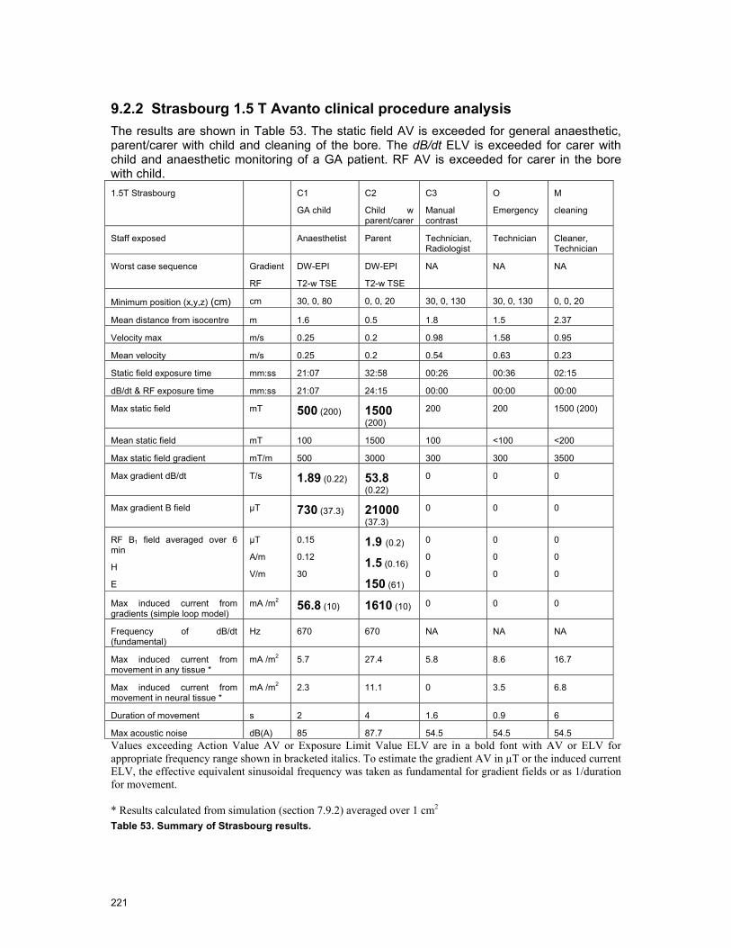
221
9.2.2 Strasbourg 1.5 T Avanto clinical procedure analysis The results are shown in Table 53. The static field AV is exceeded for general anaesthetic, parent/carer with child and cleaning of the bore. The dB/dt ELV is exceeded for carer with child and anaesthetic monitoring of a GA patient. RF AV is exceeded for carer in the bore with child. 1.5T Strasbourg C1
GA child
C2
Child w parent/carer
C3
Manual contrast
O
Emergency
M
cleaning
Staff exposed Anaesthetist Parent Technician, Radiologist
Technician Cleaner, Technician
Worst case sequence Gradient
RF
DW-EPI
T2-w TSE
DW-EPI
T2-w TSE
NA NA NA
Minimum position (x,y,z) (cm) cm 30, 0, 80 0, 0, 20 30, 0, 130 30, 0, 130 0, 0, 20
Mean distance from isocentre m 1.6 0.5 1.8 1.5 2.37
Velocity max m/s 0.25 0.2 0.98 1.58 0.95
Mean velocity m/s 0.25 0.2 0.54 0.63 0.23
Static field exposure time mm:ss 21:07 32:58 00:26 00:36 02:15
dB/dt & RF exposure time mm:ss 21:07 24:15 00:00 00:00 00:00
Max static field mT 500 (200) 1500 (200)
200 200 1500 (200)
Mean static field mT 100 1500 100 <100 <200
Max static field gradient mT/m 500 3000 300 300 3500
Max gradient dB/dt T/s 1.89 (0.22) 53.8 (0.22)
0 0 0
Max gradient B field µT 730 (37.3) 21000 (37.3)
0 0 0
RF B1 field averaged over 6 min
H
E
µT
A/m
V/m
0.15
0.12
30
1.9 (0.2)
1.5 (0.16)
150 (61)
0
0
0
0
0
0
0
0
0
Max induced current from gradients (simple loop model)
mA /m2 56.8 (10) 1610 (10) 0 0 0
Frequency of dB/dt (fundamental)
Hz 670 670 NA NA NA
Max induced current from movement in any tissue *
mA /m2 5.7 27.4 5.8 8.6 16.7
Max induced current from movement in neural tissue *
mA /m2 2.3 11.1 0 3.5 6.8
Duration of movement s 2 4 1.6 0.9 6
Max acoustic noise dB(A) 85 87.7 54.5 54.5 54.5 Values exceeding Action Value AV or Exposure Limit Value ELV are in a bold font with AV or ELV for appropriate frequency range shown in bracketed italics. To estimate the gradient AV in µT or the induced current ELV, the effective equivalent sinusoidal frequency was taken as fundamental for gradient fields or as 1/duration for movement. * Results calculated from simulation (section 7.9.2) averaged over 1 cm2 Table 53. Summary of Strasbourg results.

222
9.2.3 Leuven 3.0 T Achieva clinical sequence analysis The summary of the analysis is shown in Table 54. The EM field exposures all assume the procedures took place on the 3T scanner using data from Chapter 6. The static field AV is exceeded for tactile fMRI and cleaning. For the fMRI and GA , dB/dt exceeds the AV and dB/dt exceeds the ICNIRP limit. The current density induced by the gradients in fMRI may exceed 10 mA m-2 but interpretation of the effective frequency of the stimulus will determine compliance. Choice of axis for frequency encoding (the rapidly pulse train) in EPI is important, with the y-gradient giving the highest exposures. 3T Leuven C1
fMRI
C2
Cardiac Stress
C3
GA
O
Emergency
M
Cleaning
Staff member exposed Technician Technician Anaesthetist Technician x2 Technician x2
Worst case sequence Gradients
RF
EPI
EPI
B-TFE
B-TFE
DW-EPI
T2w-SE
NA NA
Minimum position (x,y,z) (cm) cm 30, 0, 124 90, 0, 155 20, 0, 133 20, 0, 164 0, 0, 0
Mean distance from isocentre m 1.44 1.98 4.39 1.64 -
Velocity max m/s 0.63 0.45 0.8 2.3 0.58
Mean velocity m/s 0.22 0.45 0.39 1.1 0.28
Static field exposure time mm:ss 05:50 03:00 27:42 00:19 2:29
dB/dt & RF exposure time mm:ss 05:02 03:00 21:50 00:00 00:00
Max static field mT 400 (200) 150 300 (200) 100 3000 (200)
Mean static field mT 400 (200) 150 < 3 40 3000 (200)
Max static field gradient mT/m 800 250 800 400 3500
Max gradient dB/dt T/s 0.32 (0.22)
0.53 if FE y
0.05
0.39 (0.22) 0 0
Max gradient B field µT 38.4 (30.7)
62.3 (30.7)
10
20 60 (35.2) 0 0
RF B1 field averaged over 6 min
H
E
µT
A/m
V/m
<0.034
<0.027
< 11
~0
~0
~0
<0.034
<0.027
< 11
0
0
0
0
0
0
Max induced current from gradients (simple loop model)
mA /m2 6.5
10.5 if FE y (10)
0.48
0.87
6.3 0 0
Frequency of dB/dt (fundamental) Hz 1000 240 710 NA NA
Max induced current from movement in any tissue *
mA /m2 22.7 3.0 13.8 22.7 38.9
Max induced current from movement in neural tissue *
mA /m2 9.2 1.2 5.6 9.2 15.8
Duration of movement s 1.3 2.2 1.3 0.4 3.5
Max acoustic noise dB(A) 102.9 93.6 86.4 55 55 Values exceeding Action Value AV or Exposure Limit Value ELV are in a bold font with AV or ELV for appropriate frequency range shown in bracketed italics. To estimate the gradient AV in µT or the induced current ELV, the effective equivalent sinusoidal frequency was taken as fundamental for gradient fields or as 1/duration for movement. * Results calculated from simulation (section 7.9.2) averaged over 1 cm2 Table 54.Summary of results, Leuven 3T. All values assume procedures carried out in the 3T scanner.
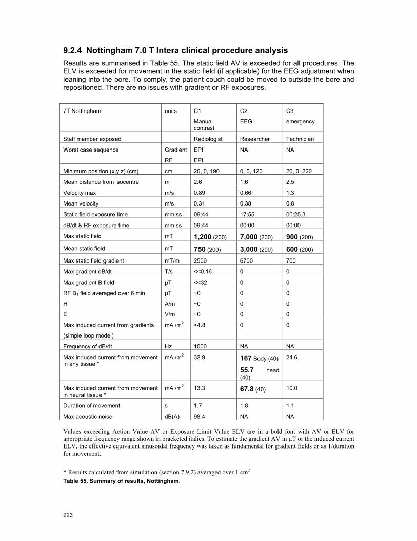
223
9.2.4 Nottingham 7.0 T Intera clinical procedure analysis Results are summarised in Table 55. The static field AV is exceeded for all procedures. The ELV is exceeded for movement in the static field (if applicable) for the EEG adjustment when leaning into the bore. To comply, the patient couch could be moved to outside the bore and repositioned. There are no issues with gradient or RF exposures.
7T Nottingham units C1
Manual contrast
C2
EEG
C3
emergency
Staff member exposed Radiologist Researcher Technician
Worst case sequence Gradient
RF
EPI
EPI
NA NA
Minimum position (x,y,z) (cm) cm 20, 0, 190 0, 0, 120 20, 0, 220
Mean distance from isocentre m 2.6 1.6 2.5
Velocity max m/s 0.89 0.66 1.3
Mean velocity m/s 0.31 0.38 0.8
Static field exposure time mm:ss 09:44 17:55 00:25.3
dB/dt & RF exposure time mm:ss 09:44 00:00 00:00
Max static field mT 1,200 (200) 7,000 (200) 900 (200)
Mean static field mT 750 (200) 3,000 (200) 600 (200)
Max static field gradient mT/m 2500 6700 700
Max gradient dB/dt T/s <<0.16 0 0
Max gradient B field µT <<32 0 0
RF B1 field averaged over 6 min
H
E
µT
A/m
V/m
~0
~0
~0
0
0
0
0
0
0
Max induced current from gradients
(simple loop model)
mA /m2 <4.8 0 0
Frequency of dB/dt Hz 1000 NA NA
Max induced current from movement in any tissue *
mA /m2 32.9 167 Body (40)
55.7 head (40)
24.6
Max induced current from movement in neural tissue *
mA /m2 13.3 67.8 (40) 10.0
Duration of movement s 1.7 1.8 1.1
Max acoustic noise dB(A) 98.4 NA NA Values exceeding Action Value AV or Exposure Limit Value ELV are in a bold font with AV or ELV for appropriate frequency range shown in bracketed italics. To estimate the gradient AV in µT or the induced current ELV, the effective equivalent sinusoidal frequency was taken as fundamental for gradient fields or as 1/duration for movement.
* Results calculated from simulation (section 7.9.2) averaged over 1 cm2 Table 55. Summary of results, Nottingham.

224
9.2.5 Measurement Summary Table 56 provides a summary of the measurement results for the four MRI scanner types, while Table 57 gives an estimate, for the highest exposure sequences measured, of the distance that workers should remain from the end of the bore not to exceed the action value. The combined uncertainty for the measurements on these scanners, for the sequences measured, is reviewed in detail within the uncertainty section. The estimated uncertainties therefore are 12% for gradient fields, 7% for RF H-field and 6% for RF E-field for the results reported in Table 34 and Table 36.
Machine Static Gradient Gradient B1 E-field B1 H-field
1.0T Panorama 1 T/m 0.32 T/s 84 V/m* 0.27 A/m*
1.5T Avanto 3.0 T/m 2 T/s 33 V/m* 0.36 A/m *
3.0T Achieva 3.5 T/m 1.7 T/s 48 V/m** 0.06 A/m*
7.0T Intera 3.0 T/m <<0.16 T/s Very small Very small
* Adjusted for the maximum available B1 field
** Enhanced by the side rail of the bed
Table 56. Maximum values measured outside the bore of static field gradient, gradient fields and RF fields.
Machine Gradient Field
exceeds the action value at the bore end by the factor
Closest approach to end of the bore not to exceed the gradient action value
RF Field exceeds the action value at the bore end by the factor
Closest approach to end of the bore not to exceed the RF action value
1.0T Panorama 1.5 40 cm 1.7 45 cm 1.5T Avanto 9.1 40 cm 2.3 20 cm 3.0T Achieva 7.3 45 cm - - 7.0T Intera - - - -
Table 57. Safe distances from the end of the bore for the measured procedures
Typically a few tens of cm from the end of the MRI scanner bore (or edge of the scanner in the case of the panorama) the stray fields have decreased below the action value (for the sequences investigated). It should be noted that for the RF fields it is the rms value averaged over 6 minutes that is important so there is both a magnitude and time element to be taken into account.
Table 58 shows a summary of the measurement results from inside the scanner bores. In all cases the action values are exceeded and in some cases by a considerable number of times, Table 59. In the case of gradient fields the instantaneous rate of change is important, but once again it should be noted that for the RF fields the rms value averaged over 6 minutes is important, so there is both a magnitude and time element to be taken into account in determining if the action value is exceeded.

225
Machine Static Gradient Gradient B1 E-field B1 H-field
1.0T Panorama ~1.5 T/m 35 T/s >140 V/m* 2.4 A/m*
1.5T Avanto n/a 40 T/s >600 V/m* 4.2 A/m*
3.0T Achieva n/a 35 T/s >360V/m* 2.4 A/m*
7.0T Intera n/a 21 T/s** 80 V/m 0.12 A/m
* Adjusted for the maximum available B1 field, maxima for measured points only (E-fields can be higher closer to the end rings of the birdcage)
**Gradient 55cm from the iso-centre.
Table 58. Maximum values measured inside the bore of static field gradient, gradient fields and RF fields.
Machine Gradient Field exceeds the action value in
the bore by the factor RF Field exceeds the action value in the bore by the factor
1.0T Panorama 160 15*
1.5T Avanto 180 26*
3.0T Achieva 160 15*
7.0T Intera 95** 1.3
* Adjusted for the maximum available B1 field, maxima for measured points only (E-fields can be higher closer to the end rings of the birdcage)
**Gradient 55cm from the iso-centre.
Table 59. The factors by which the action values are exceeded inside the bore.
The study has shown that the problematic locations with respect to occupational exposure are located very close to or inside the MRI machine. The effect of the screened room was generally negligible at those locations. It is therefore recommended that compliance evaluations with respect to safety limits for occupational EMF exposure are performed by MRI manufactures during pre-market compliance testing. For both the RF field and the gradient field measurements it is necessary to have well defined source signal set, which is only possible by the support of the MRI manufacturers e.g., for the exclusive excitation of single gradient coils with a defined pulse signal. Test-sequences should be designed in order to be representative of a worst-case scanning situation, e.g., high RF power and gradient slew rate, additionally they should be designed to support the measurement process.
It would also be beneficial for future evaluations if procedures and instrumentations for the numerical and experimental evaluations would be further optimised and standardised to obtain reliable and reproducible exposure information for workers and patients.
9.3 Conclusions Based on Observed Clinical Practice
9.3.1 Cologne 1.0 T Panorama Most conventional procedures can be completed without exceeding an action value. Leaning into the bore will exceed the static field action value. In Cologne, for the procedures observed, the anaesthetists remain outside the scanning room for monitoring of a patient under general anaesthesia. The clip insertion, using real-time guidance, exceeded static field and dB/dt action values and crudely estimated current densities exceeded the ELV by up to 15 times. The RF action values were not exceeded, but could be for a longer procedure. Current densities caused by movement within the static field (leaning into the bore) can also exceed

226
the relevant ELV due to the high static field gradients associated with this equipment. No members of staff reported any biological effect.
Detailed investigation of the dB/dt and RF exposure for the radiologist in the bore of the scanner is reported in Sections 6 and 7.
The procedure (guidewire/clip insertion) is not possible without the EM exposure of the radiologist.
9.3.2 Strasbourg 1.5 T Mid-Field System The static field AV is exceeded for GA, parent/carer with child and cleaning of the bore. The dB/dt ELV is exceeded for the carer with child, and anaesthetic monitoring of a GA patient. The RF AV is exceeded for carer in the bore with a child patient.
Detailed investigation of the carer in the bore of the magnet for dB/dt and RF is required. On occasion a member of staff may perform this role. The alternative to this practice would be to have the carer sit by the side of the bore, but this would also potentially exceed action values. An alternative is to induce general anaesthesia in the patient.
Also, the anaesthetist monitoring the patient under GA is investigated with respect to gradient field exposures (dB/dt) when observing the patient very close to the bore opening in Sections 5 to 7.
9.3.3 Leuven 3.0 T High Field System The static field AV was exceeded only for cleaning within the bore of the magnet and the tactile fMRI examination. The tactile fMRI and GA examination also resulted in exposure from the gradients exceeding the relevant AV (30.7 µT). There were no issues with movement in the static magnetic field. RF action values were not exceeded for any procedure.
The effect of the gradients in the functional MRI acquisition should be investigated further. There is no alternative to this procedure as it requires the staff member to be physically in contact with the patient.
9.3.4 Nottingham 7.0 T Ultra-High Field System The static field AV was exceeded for all procedures. For the EEG electrode adjustment, motion in the field resulted in a possible induced current density which exceeds the relevant ELV for up to 1 Hz by a factor of 2.8. There were no issues with dB/dt from the gradients or RF exposure.
Alternative arrangements could be made for the electrode adjustment, although they would involve moving the patient.
9.4 Worst Case Evaluations
In this section, an extrapolation of incident fields and exposures to the full range of MRI machines currently in use within the EU is provided. This extrapolation is based on the measured fields and simulated exposure values, the variation of the MRI machines within the study, future trends and engineering approximations, combined with the uncertainty estimations of Section 8.
The results of the evaluation providing worst-case estimates of the exposures are summarized in Table 52. The values in Table 52 express the ratio of incident field to action value or exposure to exposure limit in decibels. Decibel values in excess of 0 dB exceed the

227
action value or limit and those less than 0 dB are within the action value or exposure limit. It can clearly be seen that procedures inside the bore can result in exposures that exceed the action values by large amounts, the excedance tends to be smaller for the physical exposure limits. The uncertainties of the values are considerable due to the limited scanners investigated and the limitations of the instrumentation and access to the MR technologies. Nonetheless, the conclusions can be drawn from the findings as follows.
Action Values Physical Exposure Limits
Scanner Procedure Weighted Gradients (dB)
EB1/ELimit (dB)
HB1/Hlimit (dB)
jstatic/jlimit in CNS (dB)
jgradient/jlimit in CNS (dB)
psSARB1/ psSARlimit (dB)
wbSARB1/ SARlimit (dB)
1T Panorama
Outside the Bore (worst case)
1.1 to 9.4 2.7 to 7.3 -7.2 to 2.3
Inside the Bore (like C2)
43.1 to 51.3
4.9 to 12.5 9.5 to 17.3 22.0 to 38.3
-10.3 to 0.9
-5.5 to 3.9
1.5 Avanto
Outside the Bore (like C1)
17.0 to 25.3
-7.6 to -0.1
-7.0 to 0.8 -26 to 16 -23.2 to13.8
Inside the Bore (C2)
43.1 to 51.3
17.6 to 25.1
14.3 to 22.2 2.2 to 11.6 -1.3 to 8.1
3T Achieva
Outside the Bore
15.6 to 23.9
-5.1 to 2.4 -22.6 to14.7 6.3 - 22.6 5.8 to 22.1 - -
Inside the Bore
41.9 to 50.2
13.1 to 20.7
9.5 to 17.3 - -
7T Intera Outside the Bore
<0 <-15 <-15 - -
Inside the Bore
37.5 to 45.7
0.1 to 7.6 -16.5 to -8.7
- -
Table 60 Worst-case exposure values based on the measured values (Chapter Error! Reference source not found.) combined with the results of simulations (Chapter 6) and considering the offset uncertainty of (Chapter Error! Reference source not found.). The large offsets and uncertainties result from the very limited number of measurements and simulations. The ratios of X/Xref are given in dB, i.e., dB (X/Xref) = A log10 (X/Xref) whereby A is 10 for SAR and 20 for E. H and j.
From this we can draw the following general conclusions:
RF exposure:
• The basic restrictions regarding RF exposures based on 2004/40/EC can be met for any of the current procedures except when two persons are simultaneously inside a cylindrical bore system. Any body overlap should be avoided as it can lead to much higher exposures that considerably exceed the guidelines.
• Currently applied procedures for interventional MRI applications result in SAR values close to the SAR limits. However, the exposure could be minimized with appropriate measures (see below).
Induced Currents by Gradients and Movements:
• The basic restrictions regarding induced currents in the CNS based on the ICNIRP guidelines [9] determined according to [6] are violated for persons positioned next to the scanners by a factor of up to 10 and even more for movements.
• In the case of interventional MRI, the induced currents may exceed a factor of 100 compared to current guidelines.
228
• The prevalent cleaning procedures require the personnel to crawl inside the scanners, possibly leading to considerable induced currents.
It should be noted that the uncertainties of the computational results are significant. In many instances, they are due to strong simplifications of the numerical models of the MRI scanners. These were inevitable because (a) manufacturers were not willing to disclose complete descriptions of their coil and magnet designs and (b) the data and models provided by one manufacturer had been developed primarily to study the fields outside the bore rather than the fields inside the bore, as these are of interest in the case of most occupational exposures. Effects such as detuning of the RF coils, interaction of gradient and static fields with magnetic materials or shimming coils, etc., could not be taken into account in the simulations carried out here. On the other hand, the numerical tools and anatomical models are available to the manufacturers, and analyses of the occupational safety can be carried out by them with significantly reduced uncertainty of the scanner models.
In addition to the improved numerical models of the MR scanners, requirements to reduce the uncertainty and to better assess the variability of the exposure are:
• Advanced CAD models of the human body including, e. g., obese and pregnant models
• Tools to articulate the limbs of the models for a more realistic representation of postures during typical occupational scenarios
• Advanced numerical methods to analyze the induced temperature distribution in the body, considering blood flow and thermoregulatory effects
Acoustic Noise Exposure: The maximum measured acoustic noise value for the tested sequences was below 110 dB(A). All scanners exceeded the recommended threshold of 80 dB(A) for using hearing protectors [Directive 2003/10/EC [14]].
9.5 Recommendations
Various possibilities ranging from general exclusions for MR operations to limiting MR usage have been suggested to avoid conflict with the planned directive. Without a compromise, advancements in MR technology for beneficial medical applications might be limited. Based on our knowledge in the basis of the safety limits and dosimetry, we recommend the following measures to avoid the potential disadvantages and to foster the development of MR technology for future applications.
• Immediate initiation of targeted research to fill the knowledge gaps regarding potential hazards for these specific exposures. This will empower the standard bodies to revisit the standard and to introduce conservative limits without including extra margins for unknowns.
• Detailed and accurate information about the exposure anywhere inside the bore as well as in the vicinity of the scanner could be made available instantly (e.g., as an MR software feature). The effort/cost would be comparably small for MR manufacturers (<0.1% per device) since each coil design will require only one evaluation from which all current and future applications can be derived. This would have he benefit that any unnecessary peak exposure for patients and workers during specific MR applications could be eliminated by intelligent software control.
• Training of personnel to understand when and where peak exposures occur and how to minimize the exposure.

229
• Develop standard evaluation procedures as well as improved evaluation techniques including measurement instruments for incident field assessments and numerical tools for the dosimetric evaluations.
The authors of this report are convinced that the recommendations can be implemented within three years such that current and future MR applications are not restricted by the EU directive for workers. In the long term, the enforcement of defined and improved guidelines combined with standardized compliance procedures will result in accelerated developments of MR technology.

230
10 References
[1] FDA 2003. Criteria for significant risk investigations of magnetic resonance diagnostic devices. Rockville, MD: Center for Devices and Radiological Health, US Food and Drug Administration; July 2003.
[2] National Radiological Protection Board (1984) Advice on acceptable limits of exposure to nuclear magnetic resonance clinical imaging. Chilton, NRPB (London, HMSO)
[3] National Radiological Protection Board (1991) Principles for the Protection of Patients and Volunteers during clinical Magnetic Resonance Procedures. Documents of the NRPB Vol 2 No 1 pp1-6 (ISBN 0859513394).
[4] National Radiological Protection Board (1991) Limits on patient and volunteer exposure during clinical magnetic resonance diagnostic procedures. Documents of the NRPB Vol 2 No 1p 7-29. (ISBN 0859513394).
[5] National Radiological Protection Board (2004) Advice on Limiting Exposure to Electromagentic Fields (0-300 GHz), Documents of the NRPB vol 15,2 2004.
[6] International Electrotechnical Commission (IEC) (2002) Medical Electrical Equipment – Part 2-33: Particular Requirements for the Safety of Magnetic Resonance Equipment for Medical Diagnosis Edition: 2.0. IEC 60601-2-33. Edition 2.1 currently under review.
[7] Institute of Electrical and Electronics Engineers (IEEE) (2002) Standard for Safety Levels with Respect to Human Exposure to Electromagnetic Fields, 0–3 kHz, C95.6-2002, IEEE Inc. New York 2002
[8] Institute of Electrical and Electronics Engineers (IEEE) (2005) Standard for Safety Levels with Respect to Human Exposure to Radio Frequency Electromagnetic Fields, 3 kHz to 300 GHz -Description, C95.1-1991, IEEE Inc. New York 2005C95.1-2005; IEEE Standard for Safety Levels with Respect to Human Exposure to Radio Frequency Electromagnetic Fields, 3 kHz to 300 GHz
[9] International Commission on Non-ionising Radiation Protection.(ICNIRP) 1994 Guidelines on Limits of Exposure to Static Magnetic Fields. Health Physics 66 (1): 100-106; 1994
[10] International Commission on Non-ionising Radiation Protection.(ICNIRP) 1998. Guidelines for limiting exposure to time-varying electric, magnetic, and electromagnetic fields (up to 300 GHz). Health Phys 74 494-522.
[11] International Commission on Non-ionising Radiation Protection.(ICNIRP) (2003) Guidance on determining compliance of exposure to pulsed and complex non-sinusoidal waveforms below 100kHz with ICNIRP guidlines, Health Physics March 2003, Volume 84, Number 3, pp 383-7.
[12] International Commission on Non-ionising Radiation Protection.(ICNIRP) (International Commission on Non-ionising Radiation Protection) 2004. Medical magnetic resonance (MR) procedures: protection of patients. Health Phys 87 197-216.
[13] Directive 2004/40/EC of the European Parliament and of the Council of 29 April 2004 on the minimum health and safety requirements regarding the exposure of workers to the risks arising from physical agents (electromagnetic fields) (18th individual Directive within the meaning of Article 16(1) of Directive 89/391/EEC)
[14] Directive 2003/10/EC of the European Parliament and of the Council of 6 February 2003 on the minimum health and safety requirements regarding the
231
exposure of workers to the risks arising from physical agents (noise). (17th individual Directive within the meaning of Article 16(1) of Directive 89/391/EEC)
[15] World Health Organisation (2007) Environmental Health Criteria 238: Extremely Low Frequency (ELF) Fields. WHO, Geneva, Switzerland, ISBN 978-92-4-157238-5
[16] Barnes FS, Greenebaum B. Eds. (2007) Biological and medical aspects of electromagnetic fields. Handbook of biological effects of electromagnetic fields. 3rd edition. CRC Press Boca Raton, ISBN-10: 0849395380
[17] International Organization for Standardization. Acoustics (1990) – determination of occupational noise exposure and estimation of noise-induced hearing impairment. ISO 1999, second edition 1990.
[18] Kanal et al. (2004) American College of Radiology White Paper on MR Safety: 2004 Update and Revisions. AJR 188:1-27.
[19] Medical Devices Directorate (2002) Guidelines for Magnetic Resonance Diagnostic Equipment in Clinical Use with particular reference to Safety. 2nd edition, Medical Devices Agency, London
[20] National Radiological Protection Board (1984) Advice on acceptable limits of exposure to nuclear magnetic resonance clinical imaging. Chilton, NRPB (London, HMSO)
[21] NEMA MS 4. Acoustic Noise Measurement Procedure for Diagnosing Magnetic Resonance Imaging Devices.
[22] Bangard C, Paszek J, Berg F, Eyl G, Kessler J, Lackner K, Gossmann A (2007) MR imaging of claustrophobic patients in an open 1.0T scanner: motion artifacts and patient acceptability compared with closed bore magnets. Eur J Radiol. 64:152-157
[23] Bassen H, Schaefer DJ, Zaremba L, Bushberg J, Ziskin M, Foster KR. (2005) IEEE Committee on Man and Radiation (COMAR) technical information statement “Exposure of medical personnel to electromagnetic fields from open magnetic resonance imaging systems”. Health Phys 89 684-9.
[24] Bock M, Umathum R, Zuehlsdorff S, Volz S, Fink C, Hallscheidt P, Zimmermann H, Nitz W, Semmler W. (2005) Interventional magnetic resonance imaging: an alternative to image guidance with ionising radiation. Radiat Prot Dosimetry.117:74-8.
[25] Bradley JK, Nyekiova M, Price DL, D'jon Lopez L, Crawley T (2007) Occupational exposure to static and time-varying gradient magnetic fields in MR units. J Magn Reson Imag 26:1204-1209.
[26] Crozier S, Wang H, Trakic A, Liu F (2007) Exposure of workers to pulsed gradients in MRI, J Magn Reson Imaging 26:1236-1254.
[27] Duerk JL, Grönemeyer D, Deli M, Hum B, Kinsella A, Clifford M, Cleary K.(2000) Technical Requirements for Image-guided Spinal Procedures: workshop report on intraprocedural imaging and endoscopy.Acad Radiol. 7:971-8.
[28] Duerk JL, Wong EY, Lewin JS (2002) A brief review of hardware for catheter tracking in magnetic resonance imaging. MAGMA. 3:199-208.
[29] Elster AD. (1999) Clinical MR imaging at 8 tesla: the new frontier of ultra high field MRI.J Comput Assist Tomogr. 23:807.
[30] Gedroyc WM.(2000) Interventional magnetic resonance imaging. BJU Int. 86 Suppl .1:174-80.
232
[31] Grimm, J, Kircher, M F, Weissleder, R. (2007) Cell tracking: Principles and applications. Der Radiologe 47 25-33.
[32] Grönemeyer, D.H.W. and Lufkin, R.B. (2000) Open-Field Magnetic Resonance Imaging. Equipment, Diagnosis and Interventional Procedures. Berlin: Springer-Verlag. Berlin
[33] Hailey D. (2006) Open magnetic resonance imaging (MRI) scanners. Issues in Emerging Health Technologies, 92 1-4.
[34] Hall WA, Martin AJ, Liu H, Nussbaum ES, Maxwell RE, Truwit CL (1999) Brain biopsy using high-field strength interventional magnetic resonance imaging. Neurosurgery 44:807-813.
[35] Hall-Craggs MA.(2000) Interventional MRI of the breast: minimally invasive therapy. Eur Radiol. 10:59-62.
[36] Hashizume M. (2007) MRI-guided laparoscopic and robotic surgery for malignancies. Int J Clin Oncol. 12:94-98.
[37] Kurumi Y, Tani T, Naka S, Shiomi H, Shimizu T, Abe H, Endo Y, Morikawa S(2007) MR-guided microwave ablation for malignancies. Int J Clin Oncol. 12:85-93.
[38] Ledermann R.J. (2005) Cardiovascular interventional magnetic resonance imaging. Circulation. 112:3009-3017.
[39] Lewin JS, Nour SG, Duerk JL. (2000) Magnetic resonance image-guided biopsy and aspiration Top Magn Reson Imaging. 11:173-83.
[40] Lufkin RB, Robinson JD, Castro DJ, Jabour BA, Duckwiler G, Layfield LJ, Hanafee WN (1990) Interventional magnetic resonance imaging in the head and neck. Top Magn Reson Imaging 2:76-80.
[41] McRobbie DW , TJ Cross TJ (2005) “Occupational exposure to time varying magnetic gradient fields (dB/dt) in MRI and European limits” ISMRM MR Safety Workshop, Washington DC
[42] McRobbie D.W., Moore E. M., Graves M.J.,. Prince M.R. (2007) MRI: from picture to proton 2nd Edn, Cambridge University Press: Cambridge
[43] Mogami T, Harada J, Kishimoto K, Sumida S. (2007), Percutaneous MR-guided cryoablation for malignancies, with a focus on renal cell carcinoma. Int J Clin Oncol. 12:79-84.
[44] Moore E A , Scurr E D (2007) British association of MR radiographers (BAMRR) safety survey 2005: Potential impact of European Union (EU) Physical Agents Directive (PAD) on electromagnetic fields (EMF) J Magn Reson Imaging 26: 1303-1307.
[45] Nakada T. (2007) Clinical application of high and ultra high-field MRI. Brain Dev. 29:325-35.
[46] Regatte RR, Schweitzer ME. (2007) Ultra-high-field MRI of the musculoskeletal system at 7.0T. J Magn Reson Imaging. 25:262-9.
[47] Riches SF, Charles-Edwards GD, Shafford JC, Cole J, Keevil SF, Leach MO, (2007) Measurements of occupational exposure to switched gradient and spatially-varying magnetic fields in areas adjacent to 1.5T clinical MRI systems. J Magn Reson Imaging 26: 1346-1352.
[48] Rogers WJ, Meyer CH, Kramer CM, (2006). Technology insight: in vivo cell tracking by use of MRI. Nature Clinical Practice Cardiovascular Medicine 3 554-62
233
[49] de Senneville BD, Mougenot C, Moonen, C T W. (2007). Real-time adaptive methods for treatment of mobile organs by MRI-controlled high-intensity focused ultrasound. Magn Reson Med 57: 319-30.
[50] Bencsik M, Bowtell R, Bowley R (2007), Electric fields induced in the human body by time-varying magnetic field gradients in MRI: numerical calculations and correlation analysis. Phys. Med. Biol. 52:2337-2353
[51] Cabot E, Christ A, Oberle M, Kuster N, (2007), Local and Whole Body Exposure to RF Electromagnetic Fields of Patients Undergoing Magnetic Resonance Imaging Diagnostics, Proceedings of the 29th Annual Meeting of the Bioelectromagnetics Society, pp. 253-254, Kanazawa, Japan, June 2007.
[52] Chadwick P (2007), Assessment of electromagnetic fields around magnetic resonance imaging equipment, Technical Report, MCL-T Ltd. United Kingom, 2007.
[53] Crozier S, Trakic A, Wang Hua, Liu F,(2007) Numerical Study of Currents in Workers Induced by Body-Motion around High-Ultrahigh Field MRI Magnets, Journal of Magnetic Resonance Imaging, Magn Reson Imaging 26: 1261-1277
[54] Crozier S, Liu F (2005), Numerical evaluation of the fields induced by body motion in or near high-field MRI scanners, Progress in Biophysics and Molecular Biology, (87) 267-278
[55] Collins CM, Chronik BA, Smith MB. (2002) Development of FDTD methods for investigating peripheral nerve stimulation in MRI gradient coils. Proc. Intl. Soc. Mag. Reson. Med. 10 844.
[56] Collins C M, Liu W, Wang J, Gruetter R, Vaughan T V, Ugurbil K, and Smith M B (2004) Temperature and SAR calculations for a human head within volume and surface coils at 64 and 300 MHz J Magn Reson Imaging 19 650-656.
[57] Diehl D, Weinert U, Bijick E, Lazar R, Renz W. (2005) B1 homogenization at 3 T MRI using a 16 rung transmit array. Proc. Intl. Soc. Mag. Reson. Med. 13 2751.
[58] Gabriel C. (1996) Compilation of the dielectric properties of body tissues at RF and microwave frequencies Report N.AL/OE-TR- 1996-0037, Occupational and Environmental Health Directorate, Radiofrequency Radiation Division, Brooks Air Force Base, Texas (USA), June 1996.
[59] Gabriel C, Gabriel S, Corthout E. (1996) The dielectric properties of biological tissues: I. Literature survey. Phys. Med. Biol. 41 2231-2249.
[60] Gabriel S, Lau RW, Gabriel C. (1996) The dielectric properties of biological tissues: II. Measurements in the frequency range 10 Hz to 20 GHz. Phys. Med.. Biol. 41 2251-2269.
[61] Gabriel S, Lau RW, Gabriel C. (1996) The dielectric properties of biological tissues: III. Parametric models for the dielectric spectrum of tissues. Phys. Med. Biol. 41 2271-2293.
[62] Gandhi OP, Chen J-Y. (1992) Numerical dosimetry at power line frequencies using anatomically based models. Bioelectromagnetics 1 (suppl) 43-60.
[63] Glover PM, Bowtell R (2008), Measurement of electric fields induced in human subject due to natural movements in static magnetic fields or exposure to alternating magnetic field gradients, Physics in Medicine and Biology, 53, 361-373
[64] Hand J W, Li Y, Thomas E L, Rutherford M A and Hajnal J V (2006) Prediction of specific absorption rate in mother and fetus associated with MRI examinations during pregnancy Magn. Reson. Med. 55 883-893.
234
[65] Hanus X, Luong M, Lethimonnier F. (2005) Electromagnetic fields and SAR computations in a human head with a multi-port driven RF coil at 11.7 T. Proc. Intl. Soc. Mag. Reson. Med. 13 876.
[66] Ibrahim T S, Abduljalil A M, Baertlein B A, Lee R, and Robitaille P-M L (2001) Analysis of B1 field profiles and SAR values for multi-strut transverse electromagnetic RF coils in high field MRI applications Phys. Med. Biol. 46 2545-2555.
[67] Krietenstein B, Schuhmann R, Thoma P, Weiland T. (1998) The perfect boundary approximation technique facing the big challenge of high precision field computation. In Proc. 19th LINAC Conference, Chicago, August 1998, pp.860-862.
[68] Li, Y., Hand, J.W., Wills, T., and Hajnal, J.V. (2007) Numerically simulated induced electric field and current density within a human model located close to a z-gradient coil J Magn Reson Imaging, 26 1286-1295.
[69] Liu F, Zhao H, Crozier S (2003), Calculation of electric fields induced by body and head motion in high field MRI, Journal of Magnetic Resonance, (161) 99-107.
[70] Liu F, Zhao H, Crozier S (2003), On the induced electric field gradients in the human body for magnetic stimulation by gradient coils in MRI, IEEE Transactions on Biomedical Engineering, vol 50, no. 7, pp 804-815, July 2003.
[71] Montgomery DB, Terrell, J. (1961) Some useful information for the design of air core solenoids. National Magnet Laboratory, M.I.T. Report. AFOSR-1525, November 1961.
[72] Nadobny J, Szimtenings M, Diehl D, Stetter E, Brinkner G, and Wust P (2007) Evaluation of MR-induced hot spots for different temporal SAR modes using a time-dependent finite difference method with explicit temperature gradient treatment. IEEE Trans. Biomed. Eng. 54 1837-1850.
[73] Schuhmann R, Weiland T. (2003) Stability and conservation properties of transient field simulations using FIT. Advances in Radio Science 1 93–97.
[74] Smythe W R, Static and Dynamic Electricity, 2nd ed. (McGraw-Hill, New York, 1968). p266.
[75] So P, Stuchly MA, Nuyenhuis JA, Peripheral (2004), Nerve Stimulation by gradient switching fields in magnetic resonance imaging, IEEE Transactions on Biomedl Eng, vol. 51, no. 11, pp 1907-1914, Nov. 2004
[76] Taflove A (1995) Computational Electromagnetics - the Finite-Difference Time-Domain Method (Boston: Artech House)
[77] Vaughan J T, Hetherington H P, Otu J O, Pan J W, and Pohost G M (1994) High frequency volume coils for clinical NMR imaging and spectroscopy Magn. Reson. Med. 32 206-218.
[78] Weiland T. (1977) A discretization method for the solution of Maxwell's equations for six-component fields. Electronics and Communication (AEÜ) 31 116-120.
[79] Weiland T. (1996) Time domain electromagnetic field computation with finite difference methods. Int J Numerical Modelling 9 295-319.
[80] A. Christ et al., The Virtual Family – Development of anatomical CAD models of two adults and two children for dosimetric simulations, in preparation
[81] Wills T (2006) Development of a high resolution, anatomically realistic 3-dimensional voxel model of an adult male for use in electromagnetic radiation

235
dosimetry. Student project report, Imaging Sciences Dept, Imperial College London.
[82] Wust P, Nadobny J, Seebass M, John W, Felix R. (1993) 3-D computation of E fields by the volume-surface integral equation (VSIE) method in comparison with the finite-integration theory (FIT) method. IEEE Trans. Biomed. Eng. 40 745-759.
[83] Schuhmann R, Weiland T. (2003) Stability and conservation properties of transient field simulations using FIT. Advances in Radio Science 1 93–97.
[84] Wang H, Trakic A, Liu F, Crozier S (2008) Numerical field evaluation of healthcare workers when bending towards high-field MRI magnets Mag Reson Med 59 410-422.
[85] Floery D, Helbich TH (2006) MRI guided percutaneous biopsy of breast lesions: materials, techniques, success rates, and management in patients with suspected radiologic-pathologic mismatch Magn Reson Imag Clinics North America 14:411-425.
[86] Clasen S, Boss A, Scmidt D, Schraml C, Fritz J, Schick F, Claussen CD, Claus D, Pereira PL (2007) MR-guided radiofrequency ablation in a 0.2T open MR system: technical success and technique effectiveness in 100 liver tumors J Magn Reson Imaging 26:1043-1052.
[87] International Commission on Radiological Protection (ICRP) (2003) Basic Anatomical and Physiological Data for Use in Radiological Protection: Reference Values (Valentin J ed) Annals ICRP Publication 89, Elsevier, Amsterdam.
[88] Zhang B, Yen Y-F, Chronik BA, McKinnon GC, Scaeffer DJ, Rutt BK (2003) Peripheral nerve stimulation properties of head and body gradient coils of various sizes Magn Reson Med 50:50-58
[89] Vogt FM. Ladd ME, Hunold P, Mateiescu S, Hebrank FX, Zhang A, Debatin JF, Gohde SC (2004) Increased time rate of change of gradient fields: effect on peripheral nerve stimulation at clinical MR imaging Radiology 233:548-554.
[90] While PF, Forbes LK (2004) Electromagnetic fields in the human body due to switched transverse gradient coils in MRI. Phys Med Biol 49:2779-2798.
[91] Saunders RD, Jeffereys GR (2007) A neurobiological basis for ELF guidelines Health Phys 92:596-603.
[92] Brown MA, Martin DR, Semelka RC. (2006) Future directions in MR imaging of the female pelvis. Magn Reson Imaging Clin N Am. 2006 Nov;14(4):431-7
[93] Kuster N, Berdinas-Torres V, Nikoloski N, Frauscher M, Kainz W (2006) Methodology of detailed dosimetry and treatment of uncertainty and variations for in vivo studies, Bioelectromagnetics 27: 378-391.
[94] Taylor BN, Kuyatt CE (1994) Guidelines for evaluating and expressing the uncertainty of NIST measurement results, NIST Technical Note 1297 1994 Edition, Natl. Inst. Stand. Technol., Washington, DC 20402.

236
Appendix A Comparison of Frequency Scaling and Low Frequency (Quasi-static) Methods
A model consisting of a homogeneous sphere, conductivity 0.2 S m-1, radius 0.25 m, placed symmetrically with respect to 2 concentric current loops forming a Helmholtz pair with radii and centre-centre separation of 0.35 m was considered (Figure 231) and the current density distribution within the sphere simulated using time domain solvers (FIT and FDTD) with frequency scaling (FS) and the low frequency (LF or quasi-static QS) solver within SEMCAD. A sinusoidal current of peak amplitude 1A was assumed to flow in each loop.
Figure 231 Homogenous sphere (conductivity 0.2 S m-1) of radius 0.25 m positioned symmetrically between 2 concentric current loops forming a Helmholtz pair. The radii of the loops and their centre-centre separation were 0.35 m.
The B-field from the Helmholtz pair at a distance r off axis in the mid-plane, BHz is (Montgomery and Terrell 1961, Smythe 1968):
( )( ) ( )( )
( )
+
−++
−−
++= kKkE
a
IBHzαβα
βα
βαπ
µ41
1
122
22
220 Eq. 1
where I is the current in the loops, a is the radius of the loops, ar=α , ad=β , r is the radial distance from the axis to the field measurement point, 2d is the separation of the loops, where K(k) and E(k) are the complete elliptical integrals of the first and second kind, respectively. The current density within a homogeneous sphere exposed to a time-varying uniform B-field is given by (Smythe 1968):
( ) rBfrJ σπ= Eq. 2
where r is the radial distance (m), f is the frequency (Hz), B is the magnetic flux density (T), and s is the conductivity (S m-1).
From equation 1 the B-field magnitudes in the mid-plane (z = 0) of the Helmholtz pair, on-axis, and at 0.1 m and 0.15 m off-axis, are 2.569, 2.561 and 2.525 mT, respectively. The corresponding numerically predicted values predicted by the FIT/FS were 2.567, 2.558, and 2.521 mT.
From equation 2, with s = 0.2 S m-1, B = 2.569 mT, and f = 1 kHz, it follows that J = 161.4 mA m-2 when r = 0.1 m and 242.1 mA m-2 when r = 0.15 m. The numerical values obtained using FIT/FS at 1 kHz, for r = 0.1 m and 0.15 m, respectively, were in the range 161.09-162.47 mA m-2 (i.e. within 99.8–100.7 % of the analytical value) and 240.49–242.16 mA m-2 (i.e. within 99.3–100.04 % of the analytical value). In the latter case there was a tendency for the predicted value to underestimate slightly the analytical value; a contribution to this difference arose from the spatial variation the B-field produced by the Helmholtz pair. Values for J
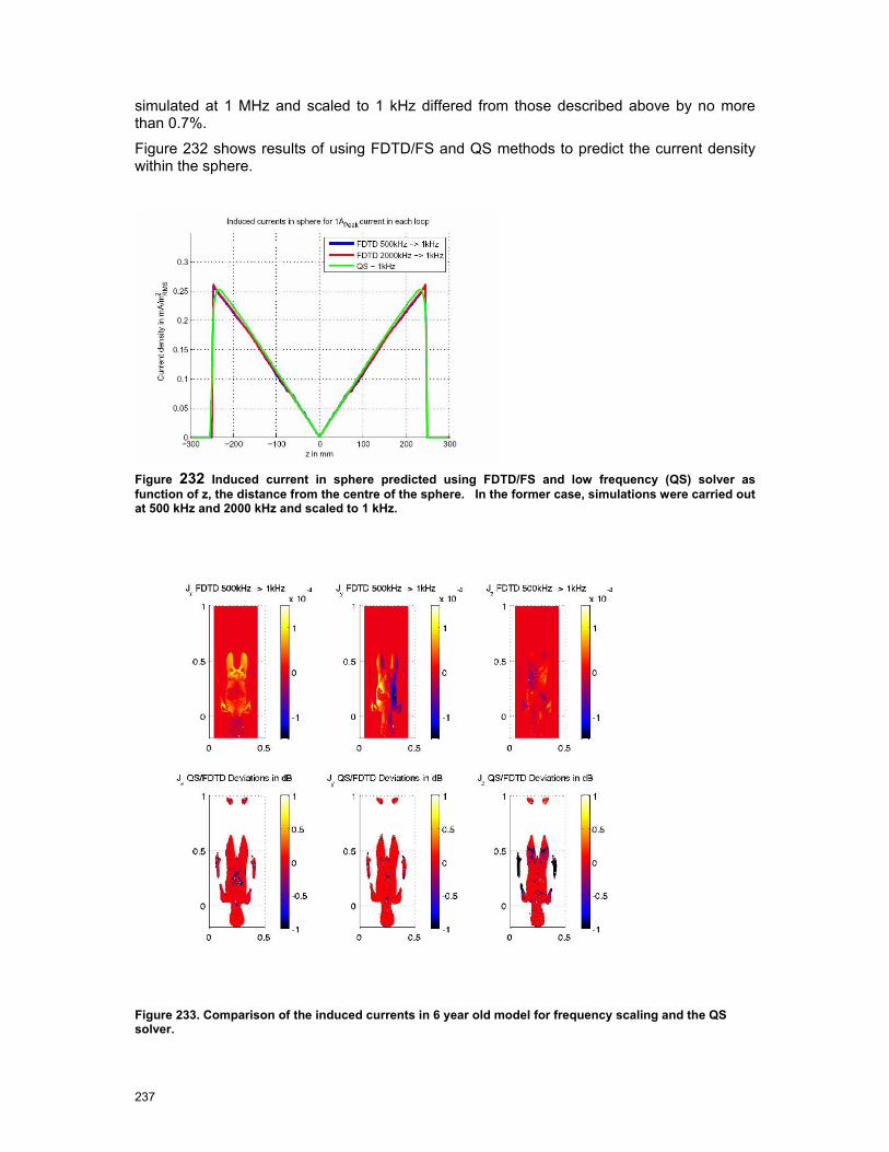
237
simulated at 1 MHz and scaled to 1 kHz differed from those described above by no more than 0.7%.
Figure 232 shows results of using FDTD/FS and QS methods to predict the current density within the sphere.
Figure 232 Induced current in sphere predicted using FDTD/FS and low frequency (QS) solver as function of z, the distance from the centre of the sphere. In the former case, simulations were carried out at 500 kHz and 2000 kHz and scaled to 1 kHz.
Figure 233. Comparison of the induced currents in 6 year old model for frequency scaling and the QS solver.

238
Appendix B
Appendix B includes:
B.1 Questionnaires (a) Cologne
(b) Strasbourg
(c) Leuven
(d) Nottingham
B.2 Acoustic Noise Protocol
B.3 Calibration Procedure for Narda ETL-400
B.4 Scan protocols (a) Cologne
(b) Strasbourg
(c) Leuven
(d) Nottingham
B.5 Radiological and Clinical Expert Panel Responses

Cologne Questionnaire
EU-PAD Questionnaire
An investigation into occupational exposure to electromagnetic fields for personnel working with
and around medical magnetic resonance imaging equipment.
Contact details: Radiological Sciences Unit, Charing Cross Hospital, Fulham Palace Road,
London, UK W6 8RF; Tel: +44 20 8846 1729
Questionnaire details
Date of questionnaire 2 August 2007........................................................................................................
Filled in by Donald McRobbie with Niels Kuster and Dr Axel Gossman.................................................
Host clinic details
Address of Clinic University of Cologne, Radiology, Building 43a, Joseph Stelzmann Str 9,
Cologne ......................................................................................................................................................
Scanner make & type: (e.g. Philips Achieva) Philips Panorama Open .............................................
Field strength 1 .........................................................................................................................................T
Workloads to be studied (e.g. interventional/paediatric/fMRI) Head/spine, breast, liver,
abdomen, MSK ..........................................................................................................................................
Interventional breast (biopsy & guidewire placement) .............................................................................
Clinical/Research/Both Both..................................................................................................................
Plans of MR suite obtained? Yes – but need fringe field contours from Philips
Scanner hardware details
Gradient system Confirm with Philips .....................................................................................................
Max gradient strength & rise time/slew rate to be confirmed .................................................................
Notes
90% interventions are for breast. Breast is the most difficult in terms of staff time near the
scanner.......................................................................................................................................................
...................................................................................................................................................................
...................................................................................................................................................................
...................................................................................................................................................................

Cologne Questionnaire
Procedure details
Procedure 1
Name of procedure Breast Biopsy .......................................................................................................
When do these happen? (e.g. Tues pm) As required..............................................................................
Number of procedures per week/month? 2-3 per week .........................................................................
Approx duration of whole procedure 45 min (30-60) ............................................................................
Which sequences are used? 3D gradient echo – but only Real time B-FFE when staff present..............
...................................................................................................................................................................
Which sequence sounds the loudest? B-FFE ...........................................................................................
Which people may be in the room during the procedure & how many? Radiologist and
technologist ................................................................................................................................................
Where would they be positioned i.e. proximity to scanner? Radiologist moves out for 3D
sequences, but if BFFE used would be present for a few seconds. Tech halfway down couch. ................
Posture e.g. standing or seated? Radiologist is seated........................................................
How long are they there for? Few seconds ..............................................................................................
If they move around – how much, where and how often? Close to bore, measured movement,
several times...............................................................................................................................................
Notes
Currently do not use real time for biopsy due to needle artefact with B-FFE but plan to change
practice. Use In-vivo receive only breast coil. Vacora Biopsy System, switching to Mammotome
MR(Suros). Will switch to real time guidance for biopsy for clinically justified reasons and
patient safety.. In using real time radiologist will be positioned within the bore. Expect significant
EM exposure. Broad measurement matrix laterally. Need to consider seated trunk.................................
...................................................................................................................................................................
...................................................................................................................................................................
...................................................................................................................................................................
...................................................................................................................................................................
...................................................................................................................................................................
Procedure 2
Name of procedure Guidewire placement (Breast)..............................................................................
When do these happen? (e.g. Tues pm) Thurs/Fri...................................................................................

Cologne Questionnaire
Number of procedures per week/month? 2 per week...............................................................................
Approx duration of whole procedure Patient ~ 30 min. Staff exposure 1-2 mins real time....................
Which sequences are used? Real-time B-FFE, single slice, 2 frames per second ....................................
...................................................................................................................................................................
Which sequence sounds the loudest? B-FFE ...........................................................................................
Which people may be in the room during the procedure & how many? Radiologist and
technologist. Tech could be outside, but radiologist leans within bore during real time scanning...........
Where would they be positioned i.e. proximity to scanner? See above. This is likely to exceed
EU action values ........................................................................................................................................
Posture e.g. standing or seated? ..Lying within bore ........................................................................
How long are they there for? 1-2 minutes................................................................................................
If they move around – how much, where and how often? Several times. Measured movements,
close to and within bore.............................................................................................................................
Notes
3D gradient echo scan done for confirmation, no one in room..................................................................
...................................................................................................................................................................
...................................................................................................................................................................
...................................................................................................................................................................
...................................................................................................................................................................
...................................................................................................................................................................
...................................................................................................................................................................
...................................................................................................................................................................
...................................................................................................................................................................
...................................................................................................................................................................

Cologne Questionnaire
Contrast Administration
Power injector available/used? Yes used always except for babies ........................................................
Number of manual per week/month? 5 per week...................................................................................
Which people may be in the room during the procedure & how many? Radiologist ..............................
Where would they be positioned i.e. proximity to scanner? See above. This is likely to exceed
EU action values ........................................................................................................................................
Posture e.g. standing or seated? ..Standing ........................................................................
How long are they there for? Duration of scan .......................................................................................
If they move around – how much, where and how often? Not required to move ....................................
GA and sedation
Is GA and or sedation performed? Yes GA babies...................................................................................
Number of manual per week/month? 5 per week but only in room if very sick.......................................
Which people may be in the room during the procedure & how many? Anaesthetist and
technician
Where would they be positioned i.e. proximity to scanner? Approx 1 m from bore entrance. May
be close for observation and ventilation ....................................................................................................
Posture e.g. standing or seated? ..Standing ........................................................................
How long are they there for? Duration of examination ...........................................................................
If they move around – how much, where and how often? As required by patient status ........................
Notes
...................................................................................................................................................................
...................................................................................................................................................................
...................................................................................................................................................................
...................................................................................................................................................................
...................................................................................................................................................................
...................................................................................................................................................................
...................................................................................................................................................................

Cologne Questionnaire
Emergency patient evacuation
Who is involved? How many staff members and which ones? 1-2 technologists. Remove couch
from bore, uncouple trolley at end.............................................................................................................
What procedures do they follow? Remove patient first. Do not attempt CPR in room ...........................
Where do they go in the room? To couch controls and end of trolley.....................................................
How long are they in the room for? Seconds ............................................................................................
Non-patient room access
Adjustment of local gradient coils (who does it/how long does it take/where do they stand etc)
Philips engineers spend a lot of time in room during scanning. Establish details with Philips ................
...................................................................................................................................................................
Description of scanner cleaning post-procedure and general (who/how long/where etc)
Dedicated, trained cleaner, under supervision..........................................................................................
...................................................................................................................................................................
Planning for further visits
Availability With 2 weeks notice can arrange for a biopsy and guidewire procedure to take place
on a single day.either Thursday or Friday. Measurements can be any weekend ......................................
Possible dates 27-28 Sept, 3-4 May Not 21 September. ..........................................................................
Access Can return key to duty radiographer for evening/night access .....................................................
Waveguide position under console LHS ................................................................................................
Electrical power in room multiple socket RH wall from console ...........................................................
Video arrangements Happy for floor marking, person in room during procedures...............................
Further Actions Formalise dates, questions for Philips ..........................................................................
Attachments:
Floor plan........................ System of work, SOPs
Fringe field plot............... MR Protocols
Photographs..................... Other

Strasbourg Questionnaire
EU-PAD Questionnaire Strasbourg
An investigation into occupational exposure to electromagnetic fields for personnel working with
and around medical magnetic resonance imaging equipment.
Contact details: Radiological Sciences Unit, Charing Cross Hospital, Fulham Palace Road,
London, UK W6 8RF; Tel: +44 20 8846 1729
Questionnaire details
Date of questionnaire 3 September 2007 ..................................................................................................
Filled in by DMcR with M Oberle, G Herbillon and Daniel VETTER......................................................
Host clinic details
Address of Clinic Radiologie, Hopital de Hautepierre, Avenue Molier, 67200 Strasbourg....................
Scanner make & type: (e.g. Philips Achieva) Siemens Avanto TIM 76/32...............................................
Field strength ............................................................................................................................................1.5T
Workloads to be studied (e.g. interventional/paediatric/fMRI) Paediatric ..............................................
...................................................................................................................................................................
Clinical/Research/Both Mainly clinical, some research............................................................................
Plans of MR suite obtained? Yes/No
Scanner hardware details
Gradient system SQ Engine .......................................................................................................................
Max gradient strength & rise time/slew rate z=45mT/m, x,y =40 mT/m, 200 mT/m/ms.......................
Notes
Software version VB13. Expecting VB15 in approx one month.................................................................
Idea Licence is available but has not been used. Test sequence would work. ...........................................
Magnetic shielding (iron) at rear of scanner.............................................................................................
...................................................................................................................................................................
...................................................................................................................................................................
Procedure details
Procedure 1
Name of procedure Paediatric GA ..........................................................................................................

Strasbourg Questionnaire
When do these happen? (e.g. Tues pm) Wed mornings ...........................................................................
Number of procedures per week/month? 4-5...........................................................................................
Approx duration of whole procedure 45 mins...........................................................................................
Which sequences are used? Various, brain, spine ,liver. Mainly brain, Includes diffusion EPI ..............
...................................................................................................................................................................
Which sequence sounds the loudest? Diffusion-EPI................................................................................
Which people may be in the room during the procedure & how many? 1 Anaesthetist, 1 nurse ..............
...................................................................................................................................................................
Where would they be positioned i.e. proximity to scanner? Close to bore. May lean in for
observation.................................................................................................................................................
...................................................................................................................................................................
Posture e.g. standing or seated?...Standing...............................................................................
How long are they there for? Whole examination.....................................................................................
If they move around – how much, where and how often? Varies, depending upon patient. ....................
...................................................................................................................................................................
Notes
...................................................................................................................................................................
...................................................................................................................................................................
...................................................................................................................................................................
...................................................................................................................................................................
...................................................................................................................................................................
...................................................................................................................................................................
...................................................................................................................................................................
Procedure 2
Name of procedure Paediatric scan no GA with parent in attendence ..................................................
When do these happen? (e.g. Tues pm) Not fixed.....................................................................................
Number of procedures per week/month? On occasion.............................................................................
Approx duration of whole procedure 30 mins...........................................................................................
Which sequences are used? Various, usually brain – T1w, T2.................................................................

Strasbourg Questionnaire
...................................................................................................................................................................
Which sequence sounds the loudest? .........................................................................................................
Which people may be in the room during the procedure & how many? Parent 1 person.........................
...................................................................................................................................................................
Where would they be positioned i.e. proximity to scanner? Lying within bore with child.......................
...................................................................................................................................................................
Posture e.g. standing or seated? ....Lying............................................................................................
How long are they there for? Duration of examnation ..............................................................................
If they move around – how much, where and how often? No movement ..................................................
...................................................................................................................................................................
Notes
This situation occurs occasionally. It is not an occupational exposure but it is of interest.......................
...................................................................................................................................................................
Alternative situation: Patient from Intesive Care on respirator. I member of staff, 1.5 m from
bore. ...........................................................................................................................................................
Not much movement. May sometime leave room during scanning............................................................
...................................................................................................................................................................
...................................................................................................................................................................
...................................................................................................................................................................
...................................................................................................................................................................
Contrast Administration
Power injector available/used? .Power injector used .............................................................................
Number of manual per week/month? .NA..............................................................................................
Which people may be in the room during the procedure & how many? .NA ..........................................
Where would they be positioned i.e. proximity to scanner? …NA ..........................................................
Posture e.g. standing or seated? …...............NA.........................................................
How long are they there for? . NA ...........................................................................................................
If they move around – how much, where and how often? .NA ................................................................

Strasbourg Questionnaire
GA and sedation
Is GA and/ or sedation performed? GA see procedure 1. Sedation sometimes – chloral hydrate ..........
Number per week/month? .Variable........................................................................................................
Which people may be in the room during the procedure & how many? …Anaesthetist………
Where would they be positioned i.e. proximity to scanner? .Half way down table ..................................
Posture e.g. standing or seated? Standing …........................................................................
How long are they there for? .Duration of examination ..........................................................................
If they move around – how much, where and how often? .Not much, view patient monitoring..............
Notes
...................................................................................................................................................................
...................................................................................................................................................................
...................................................................................................................................................................
...................................................................................................................................................................
...................................................................................................................................................................
...................................................................................................................................................................
...................................................................................................................................................................

Strasbourg Questionnaire
Emergency patient evacuation
Who is involved? How many staff members and which ones? Typ 2 techs, 1 radiologist.......................
What procedures do they follow? No written procedure ...........................................................................
Where do they go in the room? It has not happened in scanner................................................................
How long are they in the room for? This can be simulated .......................................................................
Non-patient room access
Adjustment of local gradient coils (who does it/how long does it take/where do they stand etc)
Siemens engineers go it, but not usually during scanning .........................................................................
...................................................................................................................................................................
Description of scanner cleaning post-procedure and general (who/how long/where etc)
Room is cleaned by ‘une femme de menage’ .............................................................................................
Scanner bore cleaned by technologists when required..............................................................................
Planning for further visits
Availability For video- a Wednesday morning. 3rd October good.(4 Gas) ...........................................
For measurements pos 27, 28 Oct – start Sat pm after morning session...................................................
Access A member of staff will be available ...............................................................................................
Waveguide position Under console worktop .........................................................................................
Electrical power in room Yes on LHS ....................................................................................................
Video arrangements Floor marking ok. Verbal consent is sufficient. Set up Tues pm ...........................
Further Actions Confirm dates ................................................................................................................
...................................................................................................................................................................
Attachments:
Floor plan........................ System of work, SOPs
Fringe field plot............... MR Protocols
Photographs..................... Other

Leuven Questionnaire
EU-PAD Questionnaire: Leuven
An investigation into occupational exposure to electromagnetic fields for personnel working with
and around medical magnetic resonance imaging equipment.
Contact details: Radiological Sciences Unit, Charing Cross Hospital, Fulham Palace Road,
London, UK W6 8RF; Tel: +44 20 8846 1729
Questionnaire details
Date of questionnaire 22 August 2007.........................................................................................
Filled in by DMcR with (MO, KHM) Profs Marchal, Sunaert, Van Hecke and others. In
attendance M G Herbillon. ........................................................................................................................
Host clinic details
Address Radiology, University Hospital, KULeuven, Gasthuisber,g B-3000 Leuven Scanner make & type: (e.g. Philips Achieva) Philips Achieva Quasar Dual ...........................................
Field strength ............................................................................................................................................3T
Workloads to be studied (e.g. interventional/paediatric/fMRI) Neuro (fMRI), Cardiac, possibility
of paediatrics currently carried out on 1.5T Intera. ..................................................................................
Clinical/Research/Both 80% research 20% clinical.................................................................................
Plans of MR suite obtained? Yes
Scanner hardware details
Gradient system Dual.................................................................................................................................
Max gradient strength & rise time/slew rate 40/80 mT/m, 100/200mT/m/s .............................................
Notes
Paediatrics under GA are currently performed on the 1.5T system. Possibility of videoing on both
systems. .....................................................................................................................................................
...................................................................................................................................................................
...................................................................................................................................................................
...................................................................................................................................................................
...................................................................................................................................................................
...................................................................................................................................................................

Leuven Questionnaire
Procedure details
Procedure 1
Name of procedure clinical and research fMRI – tactile stimulus ....................................................
When do these happen? (e.g. Tues pm) Any day ..................................................................................
Number of procedures per week/month? 1 per week..............................................................................
Approx duration of whole procedure 1 hour for patient. fMRI scan ~ 5 minutes....................................
Which sequences are used? BOLD EPI with TE=30ms, whole brain, 8 channel receive coil, Body
coil transmit ...............................................................................................................................................
Which sequence sounds the loudest? EPI..................................................................................................
Which people may be in the room during the procedure & how many? 1 technician/researcher
during the fMRI..........................................................................................................................................
Where would they be positioned i.e. proximity to scanner? Near bore entrance, leaning/reaching
in. For facial stimulation may be round the rear of the scanner. ..............................................................
...................................................................................................................................................................
Posture e.g. standing or seated? Standing and leaning
..............................................................................
How long are they there for? Duration of fMRI scan 5 mins. ..................................................................
If they move around – how much, where and how often? Near to bore, reaching/leaning ......................
...................................................................................................................................................................
Notes
Technician/researcher only in scanner room during fMRI scans. Door interlock disabled. ....................
This procedure can be simulated or carried out on a volunteer................................................................
...................................................................................................................................................................
...................................................................................................................................................................
...................................................................................................................................................................
...................................................................................................................................................................
...................................................................................................................................................................
...................................................................................................................................................................
...................................................................................................................................................................
Procedure 2
Name of procedure Cardiac Stress Test .............................................................................................

Leuven Questionnaire
When do these happen? (e.g. Tues pm) Currently Tues/Thurs (normally Mon/Thurs) ..........................
Number of procedures per week/month? 3 to 4 per month.....................................................................
Approx duration of whole procedure 1 hour.............................................................................................
Which sequences are used? Perfusion-EPI, cine B-TFE ..........................................................................
...................................................................................................................................................................
Which sequence sounds the loudest? B-TFE / EPI...................................................................................
Which people may be in the room during the procedure & how many? One ...........................................
...................................................................................................................................................................
Where would they be positioned i.e. proximity to scanner? Standing 40 cm from bore. ..........................
...................................................................................................................................................................
Posture e.g. standing or seated? ................................................................................................
How long are they there for? 10- 15 minutes depending upon procedure (e g dobutamine)....................
If they move around – how much, where and how often? Every minute to change infusion, watch
physiological parameters...........................................................................................................................
...................................................................................................................................................................
Notes
Currently done mainly on 1.5T but may in future migrate to 3T .
We can video procedure on 1.5T
This may be selected as a study procedure, depending upon other sites. ..................................................
...................................................................................................................................................................
...................................................................................................................................................................
...................................................................................................................................................................
...................................................................................................................................................................
...................................................................................................................................................................
...................................................................................................................................................................

Leuven Questionnaire
Procedure 3 Alternative
Name of procedure GA of a child.........................................................................................................
When do these happen? (e.g. Tues pm) Mon/Wed/Fri on 1.5T...............................................................
Number of procedures per week/month? 18 / week ................................................................................
Approx duration of whole procedure 45 min. .........................................................................................
Which sequences are used? Everything including diffusion EPI for neuro. .............................................
...................................................................................................................................................................
Which sequence sounds the loudest? Diffusion-EPI.................................................................................
Which people may be in the room during the procedure & how many? Two anaesthetists typ. ..............
...................................................................................................................................................................
Where would they be positioned i.e. proximity to scanner? Various. In the worst case they may
lean in to the scanner to view child’s chest or inspect skin colour ............................................................
...................................................................................................................................................................
Posture e.g. standing or seated? .Both..seating position at end of couch 4.5m from
isocentre..........................................................................
How long are they there for? 45 minutes ..................................................................................................
If they move around – how much, where and how often? Frequently to check on patient and
monitoring..................................................................................................................................................
Notes
Currently done mainly on 1.5T.
We can video procedure on 1.5T
This may be selected as a study procedure, depending upon other sites. ..................................................
...................................................................................................................................................................
...................................................................................................................................................................
...................................................................................................................................................................
...................................................................................................................................................................
...................................................................................................................................................................
...................................................................................................................................................................
Contrast Administration
Power injector available/used? . Yes. Used 60% of time. 40% manual (children & operational
reasons)......................................................................................................................................................

Leuven Questionnaire
Number of manual per week/month? . All children + 30 exams per week ............................................
Which people may be in the room during the procedure & how many? .technologist ............................
Where would they be positioned i.e. proximity to scanner? …50 cm......................................................
Posture e.g. standing or seated? …..standing......................................................................
How long are they there for? .1 m 30s for perfusion – longer for CE-angio sequences..........................
If they move around – how much, where and how often? .Not required.................................................
GA and sedation See procedure 3 above
Is GA and/ or sedation performed? .GA for children. No sedation..........................................................
Number per week/month? . ......................................................................................................................
Which people may be in the room during the procedure & how many? ……………………….
Where would they be positioned i.e. proximity to scanner? . ...................................................................
Posture e.g. standing or seated? …........................................................................
How long are they there for? ...................................................................................................................
If they move around – how much, where and how often? . .....................................................................
Notes
...................................................................................................................................................................
...................................................................................................................................................................
...................................................................................................................................................................
...................................................................................................................................................................
...................................................................................................................................................................
...................................................................................................................................................................
...................................................................................................................................................................
...................................................................................................................................................................

Leuven Questionnaire
Emergency patient evacuation
Who is involved? How many staff members and which ones? 1- 2 technologists ...................................
What procedures do they follow? Abort scan, evacuate patient. CPR in resus area ................................
Where do they go in the room? 50cm from bore to release couch ...........................................................
How long are they in the room for? 1 minute max.....................................................................................
Non-patient room access
Adjustment of local gradient coils (who does it/how long does it take/where do they stand etc)
Philips engineer when looking for spikes. Once or twice per year............................................................
...................................................................................................................................................................
Description of scanner cleaning post-procedure and general (who/how long/where etc)
Professional cleaner for room. Only technologists clean the scanner itself..............................................
Planning for further visits
Availability 3T scanner available during day with 2 weeks notice .........................................................
Access During day ....................................................................................................................................
Waveguide position Large WG (for projection) into equipment room .................................................
Electrical power in room Yes both side walls........................................................................................
Video arrangements Will plan to video both 1.5 and 3T Sep 24,25,26 .................................................
Further Actions Safety procedure from centre (currently in Dutch) ....................................................
Consent for videoing – draft a letter ..........................................................................................................
Obtain MR protocols
Attachments:
Floor plan........................ System of work, SOPs
Fringe field plot............... MR Protocols
Photographs..................... Other

Leuven Questionnaire

Nottingham Questionnaire
EU-PAD Questionnaire
An investigation into occupational exposure to electromagnetic fields for personnel working with
and around medical magnetic resonance imaging equipment.
Contact details: Radiological Sciences Unit, Charing Cross Hospital, Fulham Palace Road,
London, UK W6 8RF; Tel: +44 20 8846 1729
Questionnaire details
Date of questionnaire 28/8/07..................................................................................................................
Filled in by DMcR with MO and GH. Info from Paul Glover, Andrew Peters.........................................
Host clinic details
Address of Clinic The Sir Peter Mansfield MRI Centre, Nottingham School of Physics and
Astronom, University of Nottingham, Nottingham NG7 2RD....................................................................
Scanner make & type: (e.g. Philips Achieva) Philips Achieva release 2.1.3............................................
Field strength ............................................................................................................................................7T
Workloads to be studied (e.g. interventional/paediatric/fMRI) Brain only, mainly fMRI, perfusion,
study of the BOLD effect, also some spectroscopy, morphology ...............................................................
...................................................................................................................................................................
Clinical/Research/Both Research only......................................................................................................
Plans of MR suite obtained? Yes/No To be sent by Paul Glover
Scanner hardware details
Gradient system 7T gradient coil set ........................................................................................................
Max gradient strength & rise time/slew rate 33/160 currently. May increase to 40/200 in future............
Notes
No inset gradient........................................................................................................................................
No door interlock .......................................................................................................................................
Software slightly non-standard ..................................................................................................................
Adult volunteer studies only.......................................................................................................................
Procedure details
Procedure 1
Name of procedure Manual contrast injection ..........................................................................................

Nottingham Questionnaire
When do these happen? (e.g. Tues pm) – as and when project e.g. Parkinson’s or MS study.................
Number of procedures per week/month? Not specified .............................................................................
Approx duration of whole procedure 30 min typically ..............................................................................
Which sequences are used? Angio – not usually perfusion or diffusion ....................................................
...................................................................................................................................................................
Which sequence sounds the loudest? Info not available ...........................................................................
Which people may be in the room during the procedure & how many? Accompanying doctor ...............
...................................................................................................................................................................
Where would they be positioned i.e. proximity to scanner? Halfway down couch ...................................
...................................................................................................................................................................
Posture e.g. standing or seated? Standing...............................................................................
How long are they there for? 10 minutes- whole sequence......................................................................
If they move around – how much, where and how often? To bore entrance for injection ........................
Movement of head is important..................................................................................................................
Notes
This procedure only rarely done. Will attempt to schedule visit to coincide with a relevant study...........
Verbal consent from patient-volunteer will be sufficient for videoing.......................................................
...................................................................................................................................................................
...................................................................................................................................................................
...................................................................................................................................................................
...................................................................................................................................................................
...................................................................................................................................................................
Procedure 2
Name of procedure EEG experiment ........................................................................................................
When do these happen? (e.g. Tues pm) Any time ......................................................................................
Number of procedures per week/month? 1-2 per week .............................................................................
Approx duration of whole procedure not exceeding 1 hour......................................................................
Which sequences are used? BOLD-EPI, T1w for anatomical .................................................................

Nottingham Questionnaire
...................................................................................................................................................................
Which sequence sounds the loudest? EPI..................................................................................................
Which people may be in the room during the procedure & how many? Never.........................................
...................................................................................................................................................................
Where would they be positioned i.e. proximity to scanner? NA................................................................
...................................................................................................................................................................
Posture e.g. standing or seated? ......................NA..........................................................................
How long are they there for? NA .............................................................................................................
If they move around – how much, where and how often? Movement to position patient, possibly
lean in rear of bore to adjust EEG cap but not during scanning...............................................................
...................................................................................................................................................................
Notes
Patient couch is manual.............................................................................................................................
...................................................................................................................................................................
...................................................................................................................................................................
...................................................................................................................................................................
...................................................................................................................................................................
...................................................................................................................................................................
...................................................................................................................................................................
...................................................................................................................................................................
Contrast Administration
Power injector available/used? .Manual only .........................................................................................
Number of manual per week/month? .See procedure 1.........................................................................
Which people may be in the room during the procedure & how many? . See procedure 1.....................
Where would they be positioned i.e. proximity to scanner? … See procedure 1 ....................................
Posture e.g. standing or seated? …............... See procedure 1.........................................................
How long are they there for? . See procedure 1.......................................................................................
If they move around – how much, where and how often? . See procedure 1 ..........................................

Nottingham Questionnaire
GA and sedation
Is GA and/ or sedation performed? .Never...............................................................................................
Number per week/month? . ......................................................................................................................
Which people may be in the room during the procedure & how many? ……………………….
Where would they be positioned i.e. proximity to scanner? . ...................................................................
Posture e.g. standing or seated? …........................................................................
How long are they there for? ...................................................................................................................
If they move around – how much, where and how often? . .....................................................................
Notes
This procedure can be simulated if necessary ...........................................................................................
...................................................................................................................................................................
...................................................................................................................................................................
...................................................................................................................................................................
...................................................................................................................................................................
...................................................................................................................................................................
...................................................................................................................................................................
...................................................................................................................................................................

Nottingham Questionnaire
Emergency patient evacuation
Who is involved? How many staff members and which ones? 1 person, researcher ...............................
What procedures do they follow? Activate release switch on floor, unlock bed, pull out .........................
Where do they go in the room? Have to get to switch on floor by side of magnet ....................................
How long are they in the room for? 30s.....................................................................................................
Non-patient room access
Adjustment of local gradient coils (who does it/how long does it take/where do they stand etc)
Never..........................................................................................................................................................
...................................................................................................................................................................
Description of scanner cleaning post-procedure and general (who/how long/where etc)
Only by member of MR staff ......................................................................................................................
Planning for further visits
Availability Avoid wc 29 October and wc 5 Nov ....................................................................................
WC 17 Sept may be good for video visit if CE contrast study. Or wc 1 Oct. ............................................
Access Measurements can be after 5pm or weekend. A Peters will supervise ..........................................
Waveguide position Into equipment room on left. .................................................................................
Electrical power in room Yes .................................................................................................................
Video arrangements Yes, ........................................................................................................................
Further Actions A Peters to find CE-study and schedule as approp. A Glover to send field plots
and basic safety procedures to DMcR. A Peters to test RF-off procedure ................................................
Obtain MR protocols on video visit ...........................................................................................................
Attachments:
Floor plan........................ System of work, SOPs
Fringe field plot............... MR Protocols
Photographs..................... Other
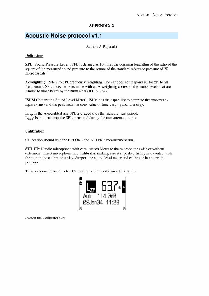
Acoustic Noise Protocol
APPENDIX 2
Acoustic Noise protocol v1.1
Author: A Papadaki
Definitions
SPL (Sound Pressure Level): SPL is defined as 10 times the common logarithm of the ratio of the
square of the measured sound pressure to the square of the standard reference pressure of 20
micropascals
A-weighting: Refers to SPL frequency weighting. The ear does not respond uniformly to all
frequencies. SPL measurements made with an A-weighting correspond to noise levels that are
similar to those heard by the human ear (IEC 61762)
ISLM (Integrating Sound Level Meter): ISLM has the capability to compute the root-mean-
square (rms) and the peak instantaneous value of time varying sound energy.
LAeq: Is the A-weighted rms SPL averaged over the measurement period.
Lpeak: Is the peak impulse SPL measured during the measurement period
Calibration
Calibration should be done BEFORE and AFTER a measurement run.
SET UP: Handle microphone with care. Attach Meter to the microphone (with or without
extension). Insert microphone into Calibrator, making sure it is pushed firmly into contact with
the stop in the calibrator cavity. Support the sound level meter and calibrator in an upright
position.
Turn on acoustic noise meter. Calibration screen is shown after start up
.
Switch the Calibrator ON.
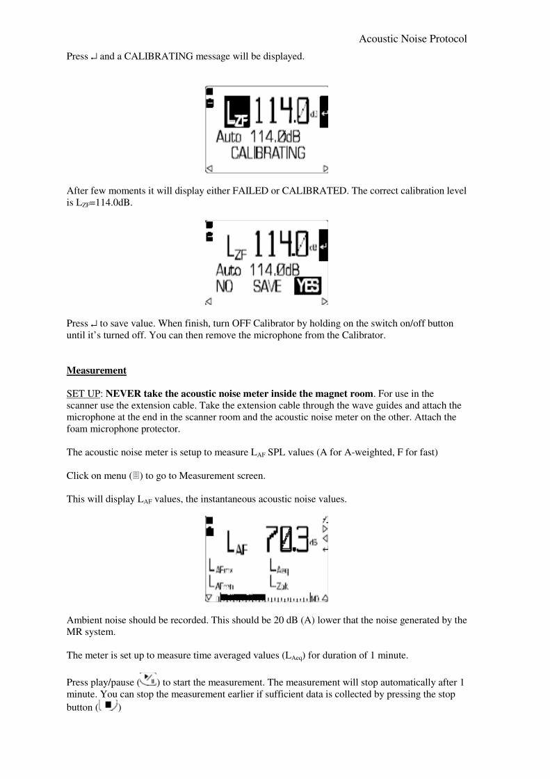
Acoustic Noise Protocol
Press ↵ and a CALIBRATING message will be displayed.
After few moments it will display either FAILED or CALIBRATED. The correct calibration level
is LZF=114.0dB.
Press ↵ to save value. When finish, turn OFF Calibrator by holding on the switch on/off button
until it’s turned off. You can then remove the microphone from the Calibrator.
Measurement
SET UP: NEVER take the acoustic noise meter inside the magnet room. For use in the
scanner use the extension cable. Take the extension cable through the wave guides and attach the
microphone at the end in the scanner room and the acoustic noise meter on the other. Attach the
foam microphone protector.
The acoustic noise meter is setup to measure LAF SPL values (A for A-weighted, F for fast)
Click on menu () to go to Measurement screen.
This will display LAF values, the instantaneous acoustic noise values.
Ambient noise should be recorded. This should be 20 dB (A) lower that the noise generated by the
MR system.
The meter is set up to measure time averaged values (LAeq) for duration of 1 minute.
Press play/pause ( ) to start the measurement. The measurement will stop automatically after 1
minute. You can stop the measurement earlier if sufficient data is collected by pressing the stop
button ( )

Acoustic Noise Protocol
Data are stored automatically under the date and time they were acquired.
View/delete stored data
Inspect data collected by pressing . Use left arrow to go to the list of stored data and scroll
using up/down arrows to select current data. Press right arrow to view header info and press
this again to view data stored.
To delete data, go to menu () and using and up/down arrows, go to Memory. Press right arrow
and select Delete current or Delete all.
Timing settings
If timing setting need to be adjusted, go to menu ()and using and up/down arrows, go to Timers,
press right arrow and select Duration Timers. Select Duration and press enter to select the time
(currently set to 1 min). To change the duration, use up/down arrows and when finish press ↵.
6, Data recorded
Site
Scanner Type
Date
Ambient Noise dB(A)
Sequence LAF max
dB(A)
LAeq
dB(A)
Duration
sec
Time of recording
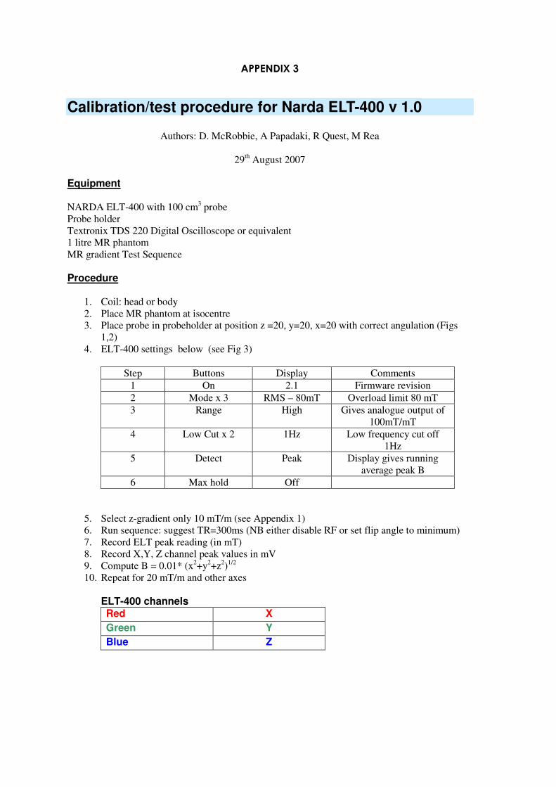
APPENDIX 3
Calibration/test procedure for Narda ELT-400 v 1.0
Authors: D. McRobbie, A Papadaki, R Quest, M Rea
29th August 2007
Equipment
NARDA ELT-400 with 100 cm3 probe
Probe holder
Textronix TDS 220 Digital Oscilloscope or equivalent
1 litre MR phantom
MR gradient Test Sequence
Procedure
1. Coil: head or body
2. Place MR phantom at isocentre
3. Place probe in probeholder at position z =20, y=20, x=20 with correct angulation (Figs
1,2)
4. ELT-400 settings below (see Fig 3)
Step Buttons Display Comments
1 On 2.1 Firmware revision
2 Mode x 3 RMS – 80mT Overload limit 80 mT
3 Range High Gives analogue output of
100mT/mT
4 Low Cut x 2 1Hz Low frequency cut off
1Hz
5 Detect Peak Display gives running
average peak B
6 Max hold Off
5. Select z-gradient only 10 mT/m (see Appendix 1)
6. Run sequence: suggest TR=300ms (NB either disable RF or set flip angle to minimum)
7. Record ELT peak reading (in mT)
8. Record X,Y, Z channel peak values in mV
9. Compute B = 0.01* (x2+y
2+z
2)
1/2
10. Repeat for 20 mT/m and other axes
ELT-400 channels Red X
Green Y
Blue Z

Results
Gradient
Strength
mT/m
Axis Expected
B (mT)
Measured
NARDA peak
(mT)
X
channel
(mV)
Y
channel
(mV)
Z
channel
(mV)
10.0 Z 2.0
20.0 Z 4.0
10.0 X 2.0
20.0 X 4.0
10.0 Y 2.0
20.0 Y 4.0
Figure 1
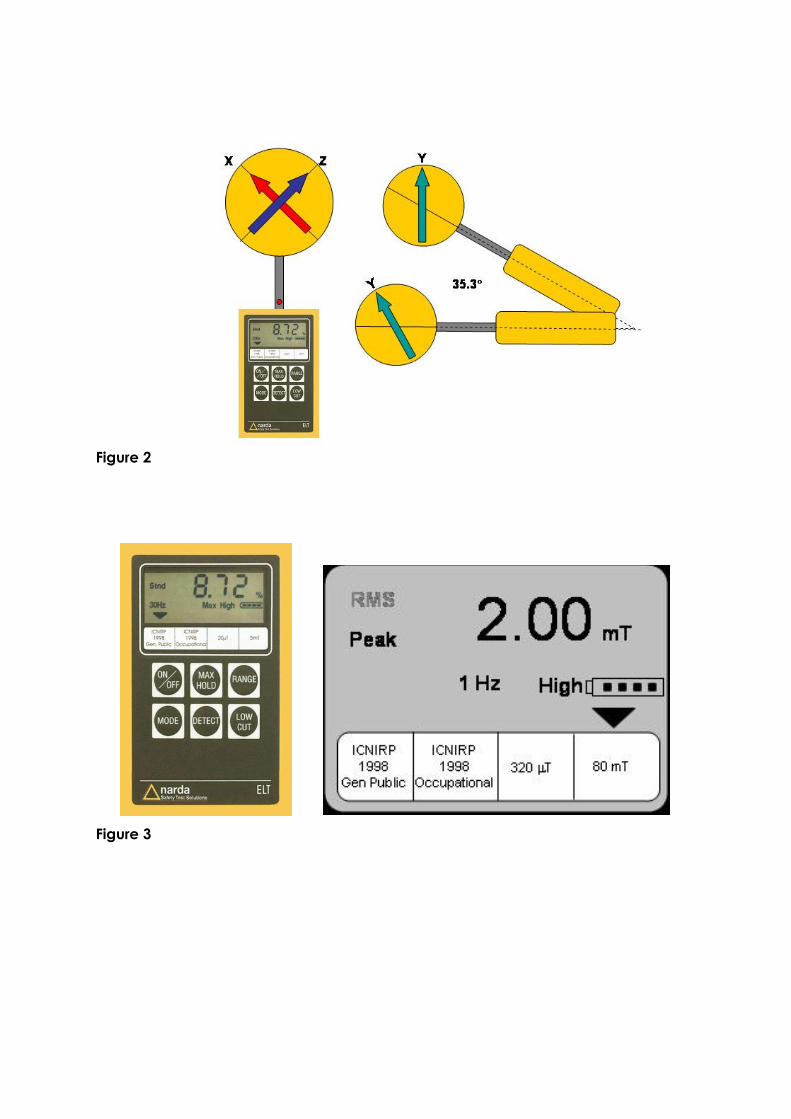
Figure 2
Figure 3

Test Sequence
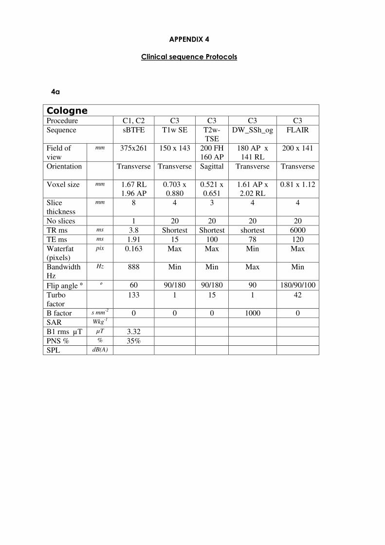
APPENDIX 4
Clinical sequence Protocols
4a
Cologne Procedure C1, C2 C3 C3 C3 C3
Sequence sBTFE T1w SE T2w-
TSE
DW_SSh_og FLAIR
Field of
view
mm 375x261 150 x 143 200 FH
160 AP
180 AP x
141 RL
200 x 141
Orientation Transverse Transverse
Sagittal Transverse Transverse
Voxel size mm 1.67 RL
1.96 AP
0.703 x
0.880
0.521 x
0.651
1.61 AP x
2.02 RL
0.81 x 1.12
Slice
thickness
mm 8 4 3 4 4
No slices 1 20 20 20 20
TR ms ms 3.8 Shortest Shortest shortest 6000
TE ms ms 1.91 15 100 78 120
Waterfat
(pixels)
pix 0.163 Max Max Min Max
Bandwidth
Hz
Hz 888 Min Min Max Min
Flip angle ° ° 60 90/180 90/180 90 180/90/100
Turbo
factor
133 1 15 1 42
B factor s mm-2
0 0 0 1000 0
SAR Wkg-1
B1 rms µT µT 3.32
PNS % % 35%
SPL dB(A)
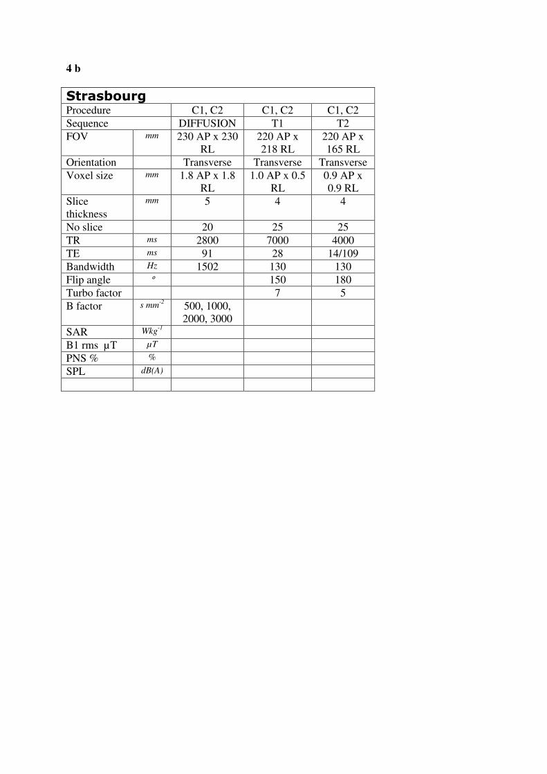
4 b
Strasbourg Procedure C1, C2 C1, C2 C1, C2
Sequence DIFFUSION T1 T2
FOV mm 230 AP x 230
RL
220 AP x
218 RL
220 AP x
165 RL
Orientation Transverse Transverse Transverse
Voxel size mm 1.8 AP x 1.8
RL
1.0 AP x 0.5
RL
0.9 AP x
0.9 RL
Slice
thickness
mm 5 4 4
No slice 20 25 25
TR ms 2800 7000 4000
TE ms 91 28 14/109
Bandwidth Hz 1502 130 130
Flip angle ° 150 180
Turbo factor 7 5
B factor s mm-2
500, 1000,
2000, 3000
SAR Wkg-1
B1 rms µT µT
PNS % %
SPL dB(A)
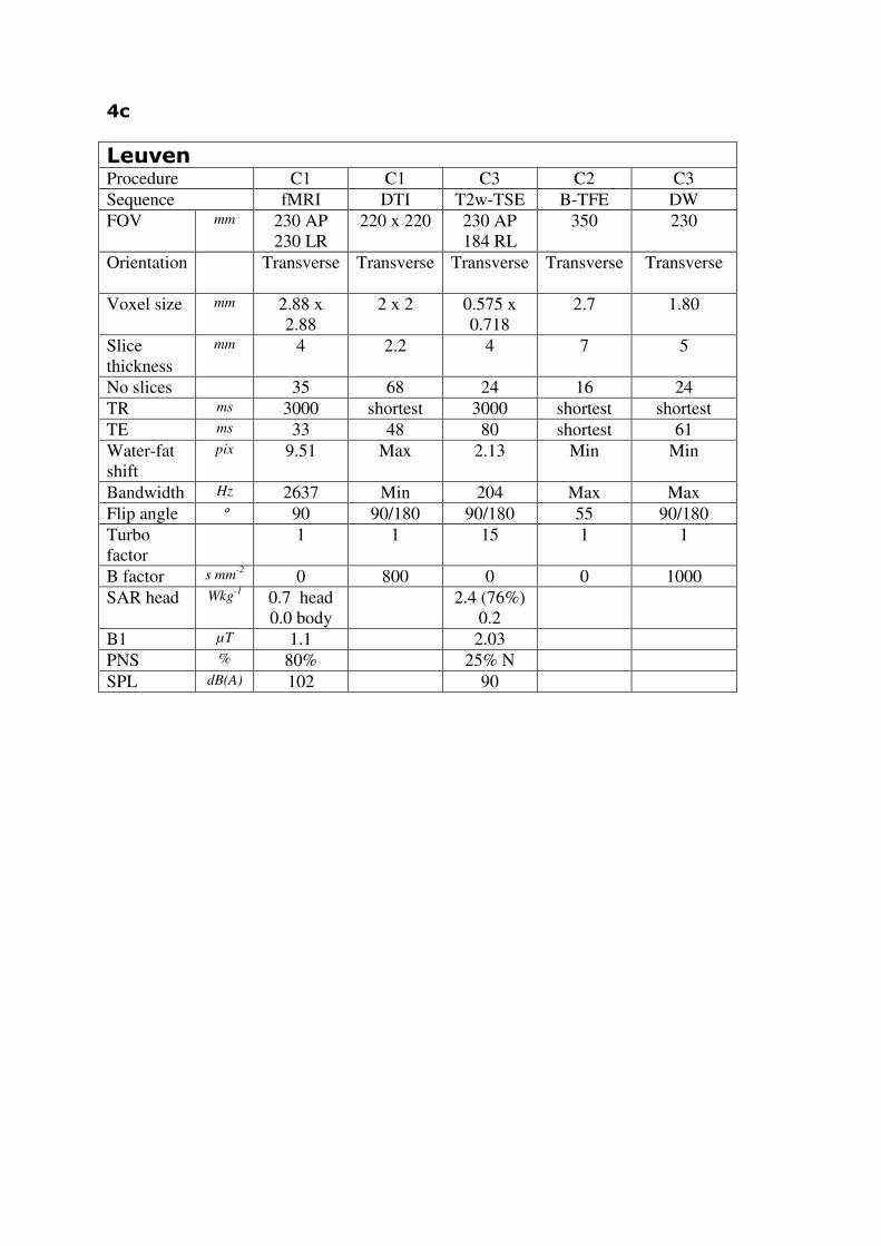
4c
Leuven Procedure C1 C1 C3 C2 C3
Sequence fMRI DTI T2w-TSE B-TFE DW
FOV mm 230 AP
230 LR
220 x 220 230 AP
184 RL
350 230
Orientation Transverse Transverse
Transverse Transverse Transverse
Voxel size mm 2.88 x
2.88
2 x 2 0.575 x
0.718
2.7 1.80
Slice
thickness
mm 4 2.2 4 7 5
No slices 35 68 24 16 24
TR ms 3000 shortest 3000 shortest shortest
TE ms 33 48 80 shortest 61
Water-fat
shift
pix 9.51 Max 2.13 Min Min
Bandwidth Hz 2637 Min 204 Max Max
Flip angle ° 90 90/180 90/180 55 90/180
Turbo
factor
1 1 15 1 1
B factor s mm-2
0 800 0 0 1000
SAR head Wkg-1
0.7 head
0.0 body
2.4 (76%)
0.2
B1 µT 1.1 2.03
PNS % 80% 25% N
SPL dB(A) 102 90

4d
Nottingham Procedure C1
Sequence fMRI
FOV mm
Orientation
Voxel size mm
Slice
thickness
mm
No slices
TR ms
TE ms
Water-fat
shift
pix
Bandwidth Hz
Flip angle °
Turbo
factor
B factor s mm-2
SAR head Wkg-1
B1 µT
PNS %
SPL dB(A)

Appendix 4 Clinical Expert Panel Responses
Professor Wladyslaw Gedroyc
Consultant Radiologist
Medical Director Magnetic Resonance Units
St Marys Hospital, Imperial College Healthcare NHS Trust
Dr Andrew Taylor
Senior Clinical Lecturer and Honorary Consultant in Cardiovascular Imaging
UCL Institute of Child Health & Great Ormond Street Hospital for Children, London
Dr Adam Waldman
Consultant Neuroradiologist, Research Director for Imaging
Imperial College Healthcare NHS Trust, London, UK
Honorary Senior Lecturer
Imperial College Faculty of Medicine & University College London

Clinical focus group – Questionnaire
Professor Wladyslaw Gedroyc
Consultant Radiologist
St Marys Hospital, Imperial College Healthcare NHS Trust
General Anaesthetic procedure
1. Did you observe the video?
Yes No
2. Was this a normal practice?
Yes No
3. If not, why?
Anaesthetists are unusually far away from their monitoring equipment. They are usually closer to the monitors.
4. Could it be carried out differently to avoid exceeding limits?
Could have only one anaesthetist in the room or outside the room with remote monitoring but this
is regarded quite rightly as being dangerous.
5. What are the alternative techniques, e.g. X-Ray, US?
n/a as depends on the GA procedure
6. Additional comments
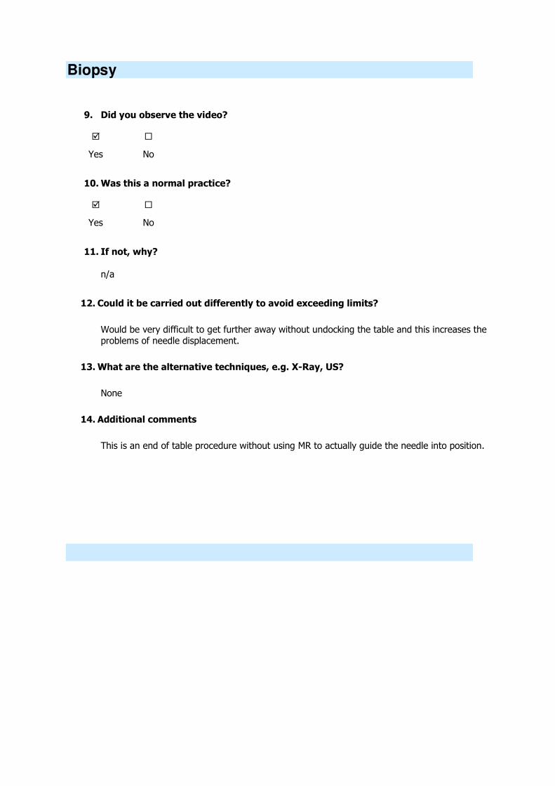
Biopsy
9. Did you observe the video?
Yes No
10. Was this a normal practice?
Yes No
11. If not, why?
n/a
12. Could it be carried out differently to avoid exceeding limits?
Would be very difficult to get further away without undocking the table and this increases the problems of needle displacement.
13. What are the alternative techniques, e.g. X-Ray, US?
None
14. Additional comments
This is an end of table procedure without using MR to actually guide the needle into position.

Clip Insertion
17. Did you observe the video?
Yes No
18. Was this a normal practice?
Yes No
19. If not, why?
n/a
20. Could it be carried out differently to avoid exceeding limits?
To place or move needles in real time the operator has to enter the scanning volume
21. What are the alternative techniques, e.g. X-Ray, US?
None
22. Additional comments
Movements here are typical and the length of time in the scanning volume was surprisingly short.

Child with parent
23. Did you observe the video?
Yes No
24. Was this a normal practice?
Yes No
25. If not, why?
Parent does not usually enter the actual core of the magnet
26. Could it be carried out differently to avoid exceeding limits?
Usually parents hold the child’s hand at either end of the bore. If the parent remains outside, the
wrong message is given to the child and failure rate is much higher.
27. What are the alternative techniques, e.g. X-Ray, US?
n/a
28. Additional comments

Other procedures
33. What other procedures may be affected by the EU limits. e.g manual contrast?
MR guided focussed ultrasound has a nurse in the room for patient reassurance and
sedation.
All interventional MR procedures e.g. laser MR guided thermal ablation.
All contrast at St Mary’s is given manually.
34. How can cleaning of the magnet be carried out to be acceptable with infection
control?
Could use wooden mops to increase the distance but this would not help much.
35. For cardiac stress test, what sequences would you use while members of staff
are inside the scanner room?
Can use remote monitors but direct patient visualisation and communication is
reduced this way.
36. Thank you for taking part in this. Would you be happy if this information is
included in our report? A copy of this will be send to you.
Yes No

Clinical focus group – Questionnaire
Andrew Taylor
Senior Clinical Lecturer and Honorary Consultant in Cardiovascular Imaging
UCL Institute of Child Health & Great Ormond Street Hospital for Children, London
General Anesthetic procedure
1. Did you observe the video?
Yes No
2. Was this a normal practice?
Yes No
3. If not, why?
Anesthetist stays outside the room in our practice (GOSH)
4. Could it be carried out differently to avoid exceeding limits?
As above
5. What are the alternative techniques, e.g. X-Ray, US?
CT – but known risk of ionizing radiation
6. Additional comments
1. Many centres will do occasional GA MR and so not be set up as we are for anaesthetist to be sat in the MR control room
2. Many cases are done under sedation, with nurse in the room. This is not to monitor, but it’s to re-assure the patient and ensure scan is successful. For this nurse has to be directly at the end of
the bore (see Sense about Science TV CH4 news document from GOSH)

Biopsy
9. Did you observe the video?
Yes No
10. Was this a normal practice?
Yes No
11. If not, why?
n/a
12. Could it be carried out differently to avoid exceeding limits?
Yes – Biopsy could be performed outside scanner if the table can be undocked without moving patient
13. What are the alternative techniques, e.g. X-Ray, US?
X-ray – no
U/S conventional (but difficult in this patient due to size)
14. Additional comments

Clip Insertion
17. Did you observe the video?
Yes No
18. Was this a normal practice?
Yes No
19. If not, why?
n/a
20. Could it be carried out differently to avoid exceeding limits?
No
21. What are the alternative techniques, e.g. X-Ray, US?
X-ray – no
U/S conventional (but difficult in this patient due to size)
22. Additional comments
In this patient no other way to do it

Child with parent
23. Did you observe the video?
Yes No
24. Was this a normal practice?
Yes No
25. If not, why?
But it may be helpful technique for getting some children into the scanner, thus avoiding GA
26. Could it be carried out differently to avoid exceeding limits?
No, if this is the way you are going to do. But conventionally, parent would be in the room sat at
the back of the scanner (exceed?)
27. What are the alternative techniques, e.g. X-Ray, US?
n/a
28. Additional comments
This would only matter if a member of staff did this repeatedly. Not an issue for a parent doing a
one off.
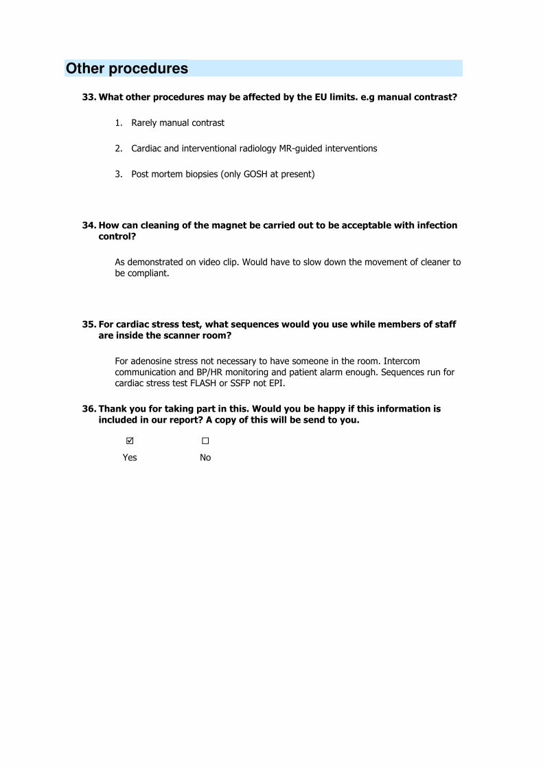
Other procedures
33. What other procedures may be affected by the EU limits. e.g manual contrast?
1. Rarely manual contrast
2. Cardiac and interventional radiology MR-guided interventions
3. Post mortem biopsies (only GOSH at present)
34. How can cleaning of the magnet be carried out to be acceptable with infection
control?
As demonstrated on video clip. Would have to slow down the movement of cleaner to
be compliant.
35. For cardiac stress test, what sequences would you use while members of staff
are inside the scanner room?
For adenosine stress not necessary to have someone in the room. Intercom
communication and BP/HR monitoring and patient alarm enough. Sequences run for cardiac stress test FLASH or SSFP not EPI.
36. Thank you for taking part in this. Would you be happy if this information is
included in our report? A copy of this will be send to you.
Yes No

Clinical focus group – Questionnaire
Adam Waldman
Consultant Neuroradiologist, Research Director for Imaging & Honorary Senior Lecturer
ICSTM and UCL
Imperial College Healthcare NHS Trust, London, UK
General Anaesthetic procedure
1. Did you observe the video?
Yes No
2. Was this a normal practice?
Yes No
3. If not, why?
n/a
4. Could it be carried out differently to avoid exceeding limits?
Anaesthetist and monitoring equipment could be in control room; but would need to enter room
intermittently to check patient (this could be problematic with regard to interlocks for some
systems)
5. What are the alternative techniques, e.g. X-Ray, US?
n/a as depends on the GA procedure
6. Additional comments
Configuration shown gives relatively low exposure as staff members are sitting some distance from the magnet bore.
Biopsy
9. Did you observe the video?
Yes No
10. Was this a normal practice?
Yes No
11. If not, why?
n/a
12. Could it be carried out differently to avoid exceeding limits?
Radiologist could be seated slightly further from the magnet. Radiographer entered room without apparent purpose.
13. What are the alternative techniques, e.g. X-Ray, US?
U/S or mammography although MRI guidance can be superior in terms of yield in some lesions.
14. Additional comments
No scanning during interventional procedure, therefore no unnecessary RF exposure, in this case.
‘Real time’ intervention would necessitate RF exposure.

Clip Insertion
17. Did you observe the video?
Yes No
18. Was this a normal practice?
Yes No
19. If not, why?
n/a
20. Could it be carried out differently to avoid exceeding limits?
Radiographer walked rapidly past magnet – could be avoided. Radiologist leant into
magnet – could be done more slowly and possibly with less exposure to field.
21. What are the alternative techniques, e.g. X-Ray, US?
U/S or mammographic (sometimes less optional depending on placement)
22. Additional comments
A change in the room configuration may potentially allow the radiologist to avoid putting
his entire upper body within the main field; however this is unlikely to make significant difference. Exposure is inevitable for this type of procedure.

Child with parent
23. Did you observe the video?
Yes No
24. Was this a normal practice?
Yes No
25. If not, why?
Not in most UK centres
26. Could it be carried out differently to avoid exceeding limits?
Patient/staff carer could comfort or support most children from outside the magnet bore. Younger
children may be sedated or given GA.
27. What are the alternative techniques, e.g. X-Ray, US?
n/a
28. Additional comments
This is not common practice in the UK and probably constitutes unnecessary exposure if the carer in
the magnet is a staff member.
Other procedures
33. What other procedures may be affected by the EU limits. e.g manual contrast?
Administration of contrast agent manually during dynamic acquisition (avoidable by
use of pump).
34. How can cleaning of the magnet be carried out to be acceptable with infection
control?
Cleaning of magnet bore could be achieved with long-handled cleaning equipment
rather than climbing into the magnet.
35. For cardiac stress test, what sequences would you use while members of staff
are inside the scanner room?
36. Thank you for taking part in this. Would you be happy if this information is
included in our report? A copy of this will be send to you.
Yes No
Extra comments
fMRI – exposure to staff depends on the paradigm used.