projected image of a cube. classical calibration
Post on 21-Dec-2015
218 views
TRANSCRIPT
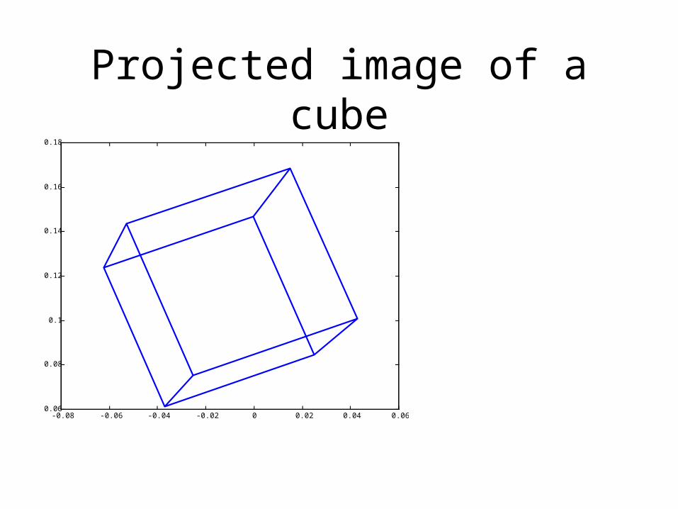
Projected image of a cube
-0.08 -0.06 -0.04 -0.02 0 0.02 0.04 0.060.06
0.08
0.1
0.12
0.14
0.16
0.18

Classical Calibration

Camera Calibration
Take a known set of points.
Typically 3 orthogonal planes.
Treat a point in the object as the World origin
Points x1, x2, x3,
Project to y1,y2,y3

Least Square Estimation: Idea
We use:

Least Square Estimation
€
ry pred = A
r x prediction
E = (y jmeasured − y j
pred
j=1
m
∑ )2 Error
E = (y jmeasured − aij x i
i=1
n
∑ )2
j=1
m
∑ Error
E = (r y meas − A
r x )t (
r y meas − A
r x ) Error Matrix form
minx
E ⇒∂E
∂x= 0 ⇒ − 2A t (
r y meas − A
r x ) = 0
⇒ A t r y meas = A t Ar x
⇒ (A t A)−1 A t r y meas =r x
In general, y is a matrix ofmeasurements, and x is a matrix of matched predictors

Converting a Matrix into a vector for Least squares…
€
y1 L ym[ ] = A x1 L xm[ ]
r y 1 L
r y m[ ] =
r a 1
t
Mr a n
t
⎡
⎣
⎢ ⎢ ⎢
⎤
⎦
⎥ ⎥ ⎥
r x 1 L
r x m[ ]
r y 1 L
r y m[ ] =
r a 1
t Lr a n
t[ ]
r x 1
r 0 L
r 0
r 0
r 0
r x 1 L
r 0
r 0
r 0
r 0 L M M
M M Lr x n
r 0
r 0
r 0 L
r 0
r x n
⎡
⎣
⎢ ⎢ ⎢ ⎢ ⎢ ⎢
⎤
⎦
⎥ ⎥ ⎥ ⎥ ⎥ ⎥
Y= X t r a 1
t Lr a n
t[ ]
t
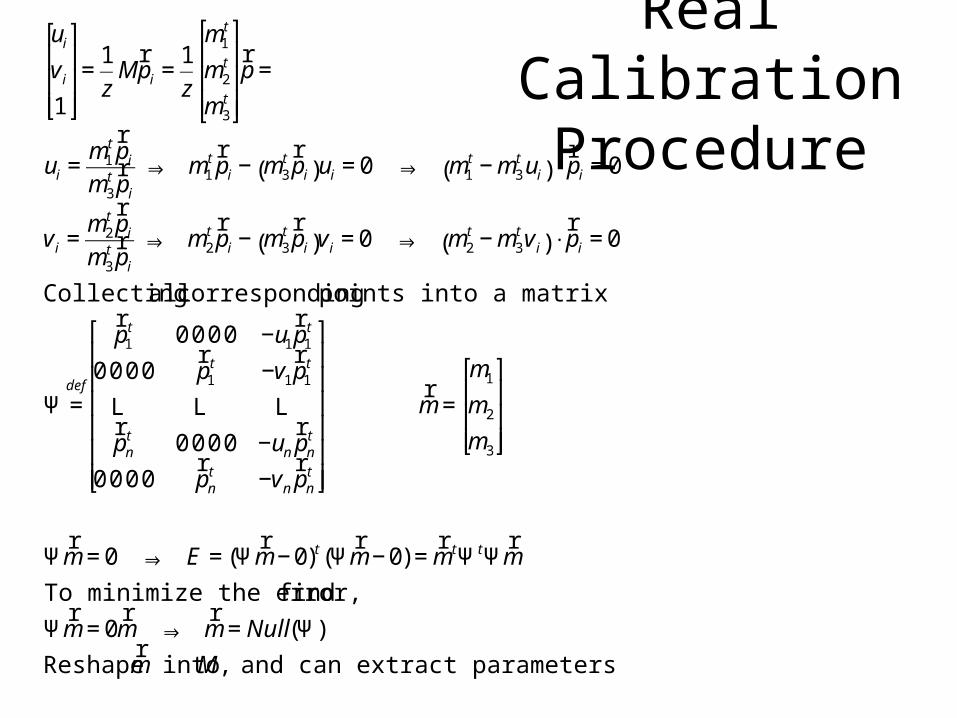
Real Calibration Procedure
€
ui
v i
1
⎡
⎣
⎢ ⎢ ⎢
⎤
⎦
⎥ ⎥ ⎥=
1
zM
r p i =
1
z
m1t
m2t
m3t
⎡
⎣
⎢ ⎢ ⎢
⎤
⎦
⎥ ⎥ ⎥
r p =
ui =m1
t r p i
m3t r p i⇒ m1
t r p i − m3
t r p i( )ui = 0 ⇒ m1
t − m3t ui( ) ⋅
r p i = 0
v i =m2
t r p i
m3t r p i⇒ m2
t r p i − m3
t r p i( )v i = 0 ⇒ m2
t − m3t v i( ) ⋅
r p i = 0
Collecting all corresponding points into a matrix
Ψ =def
r p 1
t 0 0 0 0 −u1
r p 1
t
0 0 0 0r p 1
t −v1
r p 1
t
L L Lr p n
t 0 0 0 0 −un
r p n
t
0 0 0 0r p n
t −vn
r p n
t
⎡
⎣
⎢ ⎢ ⎢ ⎢ ⎢ ⎢
⎤
⎦
⎥ ⎥ ⎥ ⎥ ⎥ ⎥
r m =
m1
m2
m3
⎡
⎣
⎢ ⎢ ⎢
⎤
⎦
⎥ ⎥ ⎥
Ψr m = 0 ⇒ E = (Ψ
r m − 0)t (Ψ
r m − 0) =
r m tΨ tΨ
r m
To minimize the error, find
Ψr m = 0
r m ⇒
r m = Null(Ψ)
Reshape r m into M, and can extract parameters from M
Multi-view geometry
• How can we recover information about the structure of an object?– Take multiple views of the object.– Each image supplies a constraint on the
location of points in space– Intersecting the constraints provides a solution

From Pinhole to Picture Plane
f’

Understanding Homogeneous Image Coordinates
(u’,v’,1)
(u,v,1)
n= (u’,v’,1) x (u,v,1)
(u,v)
(u’,v’)n
€
l =u3
v3
⎡
⎣ ⎢
⎤
⎦ ⎥⋅r n
Image

Constraint supplied by one view
(u’,v’,1)
(u,v,1)
P’= s’* (u’,v’,1)
P= s* (u,v,1)

Projective ambiguity
QuickTime™ and aYUV420 codec decompressorare needed to see this picture.
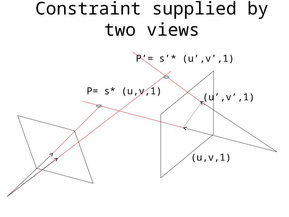
Constraint supplied by two views
(u’,v’,1)
(u,v,1)
P’= s’* (u’,v’,1)
P= s* (u,v,1)
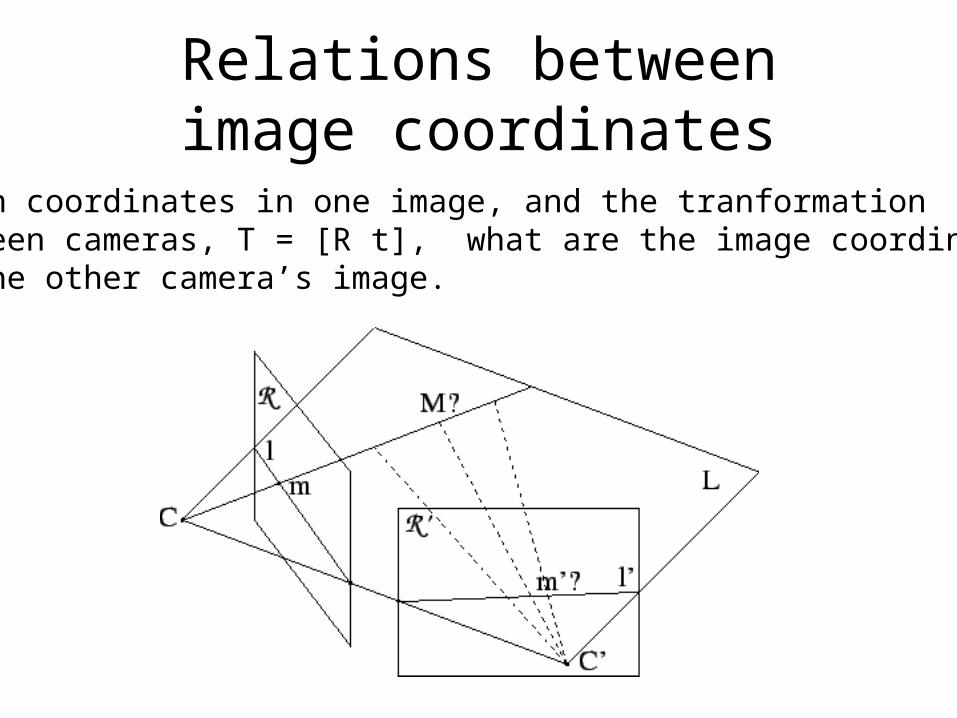
Relations between image coordinates
Given coordinates in one image, and the tranformationBetween cameras, T = [R t], what are the image coordinatesIn the other camera’s image.
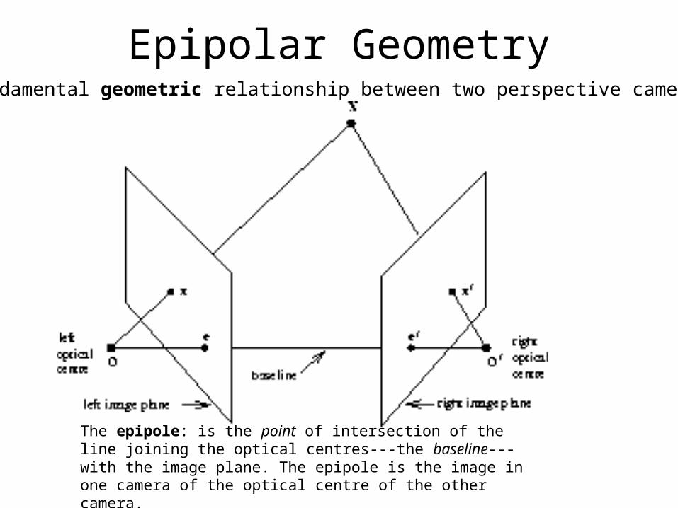
Epipolar GeometryThe fundamental geometric relationship between two perspective cameras.
The epipole: is the point of intersection of the line joining the optical centres---the baseline---with the image plane. The epipole is the image in one camera of the optical centre of the other camera.
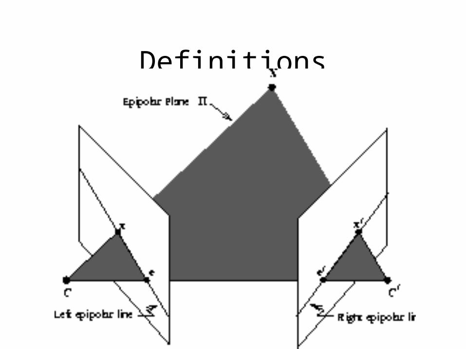
Definitions

Epipolar Example
Converging cameras

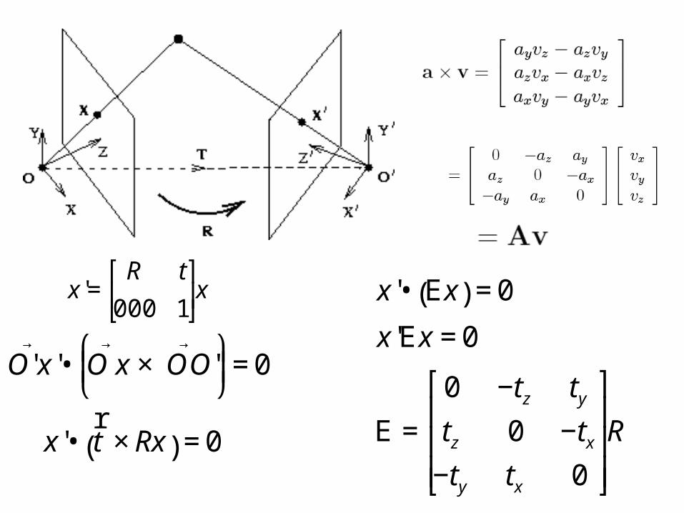
Essential Matrix: Relating between image coordinates
camera coordinate systems, related by a rotation R and a translation T:
€
O x→
O' x→
' OO'→
Are Coplanar, so:
€
x'=R t
000 1
⎡
⎣ ⎢
⎤
⎦ ⎥x€
O' x→
'• O x→
× OO'→ ⎛
⎝ ⎜
⎞ ⎠ ⎟= 0
€
x'=R t
000 1
⎡
⎣ ⎢
⎤
⎦ ⎥x
€
x'•r t × Rx( ) = 0
€
O' x→
'• O x→
× OO'→ ⎛
⎝ ⎜
⎞ ⎠ ⎟= 0
€
x'• E x( ) = 0
x'E x = 0
E =
0 −tz ty
tz 0 −tx
−ty tx 0
⎡
⎣
⎢ ⎢ ⎢
⎤
⎦
⎥ ⎥ ⎥R

What does the Essential matrix do?
It represents the normal to the epipolar line in the other image
€
n = E x
xon epipolar line' ⇒ n ⋅ x ' = 0
n1x1 + n2x2 + n31 = 0
y = mx + b( )⇒ b = −n3, m = −n1
n2
The normal defines a line in image 2:

What if cameras are uncalibrated? Fundamental Matrix
Choose world coordinates as Camera 1. Then the extrinsic parameters for camera 2 are just R and tHowever, intrinsic parameters for both cameras are unknown.Let C1 and C2 denote the matrices of intrinsic parameters. Then the pixel coordinates measured are not appropriate for the Essential matrix. Correcting for this distortion creates a new matrix: the Fundamental Matrix.
C=
€
x'measured = C2x ' xmeasured = C1x
x '( )tE x = 0⇒ C2
−1x 'measured( )tE C1
−1xmeasured( ) = 0
x 'measured( )tF xmeasured = 0
F = C2−tEC1
−1
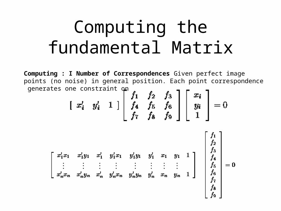
Computing the fundamental Matrix
Computing : I Number of Correspondences Given perfect image points (no noise) in general position. Each point correspondence generates one constraint on