projection techniques for document maps - moritz...

Bachelor’sThesis

ProjectionTechniquesforDocumentMaps

Moritz Stefaner

September 2005

University of Osnabrück

Cognitive Science Program

Supervisors:

Dr. Petra Ludewig

Dr. habil. Helmar Gust

Contents

...........................................................................ListofAbbreviations 4

1. ........................................................................................Introduction 5

2. ...................................Context:Creationanduseofdocumentmaps 62.1. ..................................................................................................Mapstoday 6

2.1.1. ..............................................................................................Traditionalmaps 7

2.1.2. ............................................................................................Mapasmetaphor 7

2.2. .............................DocumentmapsinInteractiveInformationVisualization 9

2.3. ...................................................DocumentmapsinInformationRetrieval 10

2.4. ....................................................Techniquesforcreatingdocumentmaps 11

2.4.1. .................................................................................Query-documentmaps 12

2.4.2. ..........................................................................................................Biplots 13

2.4.3. .....................................................................................Documentnetworks 14

2.4.4. ......................................................................................Clustervisualization 14

2.4.5. ..................................................................................Self–OrganizingMaps 15

2.4.6. ............................................................Advantagesofprojectiontechniques 16

3. .......................Analysis:2Dprojectionsofdocumentvectorspaces 173.1. ........................................Datapreparationanddocumentrepresentation 17

3.1.1. ..................................Thevectorspacemodelfordocumentrepresentation 18

3.1.2. .........................................................................Reducingthedimensionality 19

3.1.2.1. .....................................................................................Linguisticpreprocessing 20

3.1.2.2. ................................................................................................Featureselection 21

3.1.2.3. .......................................................................................Featuretransformation 23

3.2. ....................................................................................Similaritymeasures 25

3.2.1. ........................................................................................Euclideandistance 25

3.2.2. ...................................................................................Mahalanobisdistance 26

3.2.3. ............................................................................................Cosinesimilarity 26

3.2.4. ...............................................................................................Normalization 26

3.3. ................................................................................Projectiontechniques 27

3.3.1. .............................................................PrincipalComponentAnalysis(PCA) 28

3.3.2. ................................................................Multi–DimensionalScaling(MDS) 29

3.3.3. ..............................................................................MDS–relatedtechniques 32

3.3.3.1. ..............................................................................................Springembedding 32

3.3.3.2. ...............................................................CurvilinearComponentAnalysis(CCA) 32

3.3.3.3. ....................................................Isomap&CurvilinearDistanceAnalysis(CDA) 33

3.3.3.4. .....................................................................RelationalPerspectiveMap(RPM) 34

3.4. ..................................................................................................Discussion 34

3.5. .........................................................................................Empiricalresults 36

4. ..............................................Synthesis:Fromcoordinatestomaps 404.1. ............................................................................Cartographictechniques 40

4.2. .........................................................................................Mapinteraction 42

4.3. ....................................................................................TheASADOsystem 43

4.4. ..................................................................................................Discussion 45

...........................................................................................Literature 47

........................................................................................Declaration 50

ListofAbbreviations

Abbreviations used in this thesis:

CCA

CDA

ICA

IDF

LSA

LSI

MDS

PCA

POI

RPM

SOM

SVD

TF

TFIDF

Curvilinear Component Analysis

Curvilinear Distance Analysis

Independent Component Analysis

Inverse Document Frequency

Latent Semantic Analysis

Latent Semantic Indexing

Multi–Dimensional Scaling

Principal Component Analysis

Point of Interest

Relational Perspective Map

Self–Organizing Map

Singular Value Decomposition

Term Frequency

Term Frequency – Inverse Document Frequency

1. Introduction

In this work, vector space projection techniques for creating two–dimensional maps of

text document collections are presented and compared.

Document mapping is a recently developed sub–discipline of interactive information

visualization. The core idea is to combine traditional cartographic techniques with today’s

possibilities for automated analysis of text data in an interactive interface. It is hypothe-

sized that this form of presentation for text documents facilitates a quick perception of the

similarity of their contents. Hence, it can constitute a valuable addition to traditional

browsing and search methods.

Numerous techniques for creating these maps have been developed, like cluster visualiza-

tion or document networks. This work presents methods which calculate a coordinate

configuration in two–dimensional space in order to express inter–document similarities

via spatial proximity. We can distinguish algebraic methods like Principal Component

Analysis and neural training methods like Multi–Dimensional Scaling and its variants. Both

theoretical properties and empirical findings are discussed.

Some of the presented techniques have been implemented in the ASADO system1 , which

is presented at the end of this work; a demo version is available for download at

http://der-mo.net/ASADO.


5

1 The ASADO system was designed and produced in the context of the study project ASADO at the Universities of Osnabrück and Hildesheim in cooperation with the aircraft manufacturer AIRBUS.

2. Context:Creationanduseofdocumentmaps

"[...] What do you consider the largest map that would be really useful?"

"About six inches to the mile."

"Only six inches!" exclaimed Mein Herr. "We very soon got to six yards to the

mile. Then we tried a hundred yards to the mile. And then came the grandest idea

of all! We actually made a map of the country on the scale of a mile to the mile!"

"Have you used it much?" I enquired.

"It has never been spread out, yet," said Mein Herr: "the farmers objected; they

said it would cover the whole country and shut out the sunlight! So we now use

the country itself, as its own map, and I assure you it does nearly as well."

Lewis Carroll, Sylvie and Bruno Concluded (Carrol, 2005)

2.1. Mapstoday

The information and communication explosion of the digital age changes both domain

and methods of map–making. The need for coherent and efficient data presentation

grows, as the sheer amount of available information exceeds classical techniques for in-

formation access and storage.

Consequently, the now feasible exploration of large high–dimensional data sets in real–

time has resulted in new visualization techniques. Another substantial difference to

classical media is the interactivity of digital media, which allows direct interaction with

information graphics. In this context, cartography and the concept of a map are

undergoing a transformation.


6

2.1.1. Traditionalmaps

Traditional definitions like

“Graphic representation, drawn to scale and usually on a flat surface, of fea-

tures—usually geographic, geologic, or geopolitical—of an area of the Earth or of

any celestial body.” (Encyclopedia Britannica, 2005)

stress the original, geographic (or astronomic) usage of maps.

Such a map in the narrow sense usually has the following properties:

• The map is an abstract external representation of an actual physical configuration. A

map is not supposed to merely depict reality — as humorously hinted at in the in-

troductory quote — but to highlight and add information.

• Every point on the map can be connected to a point in the source domain, and

neighboring regions on the map correspond to neighboring regions in the source

domain — the map is continuous.

• Consequently, there is a monotonous relation between inter–point distances on the

map and in reality. If there exists a linear relation, typically a scale is supplied to

indicate the scaling factor of the map.

Optional features of maps in the narrow sense include direction information (e.g. by an

indication of the north direction), labels for landmarks or areas and additional information

connected to points or areas on the map (like statistical information). The presence of the

latter feature makes a map a cartogram.

2.1.2. Mapasmetaphor

Today, information graphics are increasingly used to display qualitative and quantitative

information by using a map metaphor or single techniques borrowed from classical maps.

Figure1:TheLondonUndergroundmap


7

One example is the hybrid diagram map frequently used for metro plans (see figure 1).

The map displays stations connected by metro lines; metro lines are differentiated by the

use of color. The on–map positions of the station symbols is loosely connected to the ac-

tual spatial location — however, neither distances nor exact locations are faithfully pre-

served, since the primary goal of this information graphics is the display of relational in-

formation between places in a space–efficient and visually appealing manner. The spatial

configuration is only preserved in a topological and not in a metric sense. It is worthwhile

to note that the whitespace between the stations and lines cannot be connected to actual

physical points – this kind of map is not continuous.

Figure2:Anexampleknowledgemap2

A borderline case might be found in knowledge maps (sometimes also referred to as mind

maps or concept maps; see figure 2). These are used to organize abstract information items

in a spatial manner. Again, the basic elements are nodes and relations3 , which might make

a classification as a graph diagram the prima facie choice. But again, the spatial configura-

tion is not arbitrary; rather, spatial proximity on the map is often supposed to reflect se-

mantic proximity of the associated items. From this perspective, the diagram becomes a

map of an abstract information space.


8

2 retrieved fromhttp://www.conceptdraw.com/products/img/ScreenShots/minmdap/CustomerServiceTraining.gif

3 This underlying graph structure is not always well reflected in the representation. Figure 2 shows a mindmap, where apparently only one node in the center is present and the rest of the map consists of labeled edges. However, structurally, these should have the status of a node, since they represent entities with properties and relations to other entitites.

To sum up, maps in the wider sense vary widely with respect to the objects displayed, the

mapping techniques used and the kind of information conveyed. Any of these map types

might be used for a document visualization. A minimal defining principle for maps in the

wider sense — compared to other kinds of information graphics — might be, what Waldo

Tobler called4 the First Law of Geography: “Everything is related to everything else, but

closer things are more closely related”.

2.2. DocumentmapsinInteractiveInformationVisualization

Creating maps of document spaces differs greatly from traditional cartography concerning

domain and techniques. Typically, it is attributed to the quite novel discipline of Informa-

tion Visualization.

The principal idea in visualization in general is to take advantage of our powerful visual

system to efficiently process complex information. Visual information can be processed in

parallel, automatically, and unconsciously. Thereby, it can be used to “bypass the bottleneck

of human working memory” (Zhang et al., 2002, p.1). Given an adequate visual representa-

tion of the data, characteristics of the data can be perceived directly without active inter-

pretation and deliberation. The resulting information graphics can not only be used to

store, but also to discover information.

The discipline of Information Visualization aims at the latter, exploratory purpose: It can

be defined as the use of computer–supported, interactive visual representations of ab-

stract data to amplify cognition (Card et al.,1999). Hence, the general aim is to automati-

cally calculate interactive information graphics as tools for thinking or in order to facilitate

knowledge discovery. This is in contrast to the representational, illustrative purpose of

hand–crafted information displays graphics used over the last centuries in visualization.

Many taxonomies have been developed to classify the variety of interactive visualization

techniques systematically. Among the most prominent ones are Ben Shneiderman’s task–

oriented “Task by Data Type Taxonomy” (Shneiderman, 1996), Card and Mackinlay’s taxon-

omy based on data types (Card & Mackinlay, 1997) and Keim and Kriegel’s display–mode

classification (Keim & Kriegel, 1996). Without going into the specifics of these models, suf-

fice it to remark that maps and map–like displays constitute an integral part in all of these

taxonomies.

Clearly, the automization of a very specialized skill like cartography — requiring high

technical, aesthetical and empathic capabilities on side of the map–maker — is not an easy


9

4 according to (Skupin, 2000)

task. Some challenges can be overcome, however, by the interactivity of the medium: the

possibility of integrating the user’s actions with an immediate adaptation of the resulting

display opens up a whole new dimension of possibilities. Compared to the creation of a

static map, this results in very different usage scenarios and demands on the visualization.

In this light, the creation of interactive maps has to be seen as a discipline of its own —

sharing some techniques with traditional cartography and scientific visualization, but dif-

fering in method, aim and domain.

2.3. DocumentmapsinInformationRetrieval

One of the central fields of activity for interactive information visualization is the broad

area of Information Retrieval. Especially the advent of the world wide web and digital

libraries and catalogues require the development of novel methods to find and access in-

formation stored in documents.

Currently, the predominant technique for information access in unknown document col-

lections is a keyword search with a relevance–ranked list as a result. This works well, if

the query terms are unambiguous and the user can formulate a well–defined query. How-

ever, if the search does not deliver the desired results or a too heterogeneous document

collection, it is up to the user to formulate a better–fitting query. Similar problems arise if

only vague ideas exist about the documents of interest or due to lexical ambiguities.

Ranked lists clearly are an effective way to display data ordered by a linear property —

such as relevance to a query or the date of creation of a document. However, they are not

suited well to display the complex relationships within the retrieved document set or to

support exploratory browsing. It constitutes a less directed activity, typically aimed at

gaining overview over a document collection or identifying documents of interest without

a clear preconception. The tools provided are normally document organisation structures

like hierarchical folder structures, annotated catalogues, facetted meta–data classification

or hyperlinks between documents.

Often, the motives and information needs during one retrieval session alternate. Conse-

quently, tools providing both facilities for directed access and exploratory activity are ex-

pected to be most useful. (Lagus, 2002)

The cluster hypothesis states that “closely associated documents tend to be relevant to the

same requests […, in turn,] relevant documents tend to be more similar to each other than to

non–relevant documents” (Hearst & Pedersen, 1996, p.2).5 Findings from information for-

aging theory support and refine this claim by identifying typical information seeking

strategies comparable to animals’ food and mate seeking behavior (Pirolli & Card, 1998). A


10

5 Of course, this only holds for a query–relative notion of similarity.

central notion here is “information scent”, which denotes the cues given to guide a user on

his track to the desired results. Again, it is assumed that relevant documents are likely to

be found in the vicinity of other relevant documents.

Given these findings, it becomes evident that some information retrieval tasks can greatly

benefit if the user is enabled to inspect the inner similarity structure of a retrieved

document set. First, this facilitates an initial overview of the coarse structure of the result

set to identify subgroups and outliers. Further, once a good hit has been identified, users

can find further relevant documents more easily by browsing its similarity neighborhood.

And moreover, experienced users can instantly evaluate the quality of their search terms

supported by visual cues, e.g. how shattered the result set is presented and how clearly

clusters are separated.

Maps and map–like displays are a premier candidate to display inter–document similarity

structure: The map metaphor is well–known to all users from everyday life. Hence, a

plethora of cartographic techniques can be utilized without the need of explanation. It has

been shown that the distance–similarity metaphor is adopted effortlessly (Montello et al.,

2003). Moreover, navigation has become the predominant metaphor of hypermedia (Sku-

pin, 2000), which further facilitates the introduction of spatial metaphors in document

presentation.

2.4. Techniquesforcreatingdocumentmaps

One popular approach to document mapping — and the focus of this work — is to create a

two–dimensional coordinate configuration such that inter–document similarities are en-

coded in spatial proximity. These will be referred to as projection techniques in the fol-

lowing.

Figure 3 demonstrates schematically, how a document map based on the coordinate infor-

mation could be presented, in conjunction with additional meta–data and cluster structure

information. A common metaphor is the encoding of local map distance distortion via a

relief structure, resulting in island and mountain impressions. The real distance between

two points is supposed to larger in darker areas; in figure 3, this would mean that the

cluster on the top left is even more distant to the other two clusters than in a linear prox-

imity–to–similarity mapping.


11

Of course, a variety of other mapping paradigms for document sets have been developed.

Some exemplary alternatives to the presented approach shall be discussed in the following

section:

• Query–document maps and biplots can be used to visualize documents’ properties,

such as their relation to the query terms or meta–data.

• For the display of inter–document similarity, document networks, cluster visuali-

zation and Self–Organizing Maps are frequently encountered solutions.

The taxonomy used to classify the solutions and some more examples can be found in

(Zamir, 2001).

2.4.1. Query-documentmaps

One of the earliest document visualization solutions was the VIBE system (Olsen et al.,

1991), in which documents are arranged with respect to user–defined reference points

(Points of Interest, abbr. POI). These reference points can either represent query terms or

other important concepts with respect to the document set. The coordinates are computed

by a weighted sum of the POI vectors based on the similarity values or approximated in a

physically motivated spring–embedding approach, where higher similarity corresponds to

stronger virtual springs between document and POI.

Group!of!similar!documents(cluster)

Landmark!(e.g.!query!term)

Relief!structureindicates

distance!distortion

Figure3:Adocumentmapbasedon

inter–documentsimilarity


12

Although useful for indicating the relation of documents to search terms, keywords or

reference documents, it is problematic that a document’s position might be ambivalent

(see figure 4). Clearly, document 7 is strongly related to POI C and D and not to the other

POI. However, there are several reasons why document 2 in the above figure might have

been put at its specific position — e.g. similarity to A and D, or E and B etc. Consequently,

the visual cluster composed of documents 3 to 6 might consist of very different documents

which happened to be put in similar places for different reasons.

2.4.2. Biplots

A second method which exploits document properties rather than document relations is

the scatterplot (in the two–dimensional case also referred to as biplot). The displayed

space is spanned by two axes with a pre–defined semantics. Accordingly, any point on the

cartesian plan is associated with two variable values. This kind of visualization is both

useful to inspect the co–distribution of two variables as well as for quickly filtering value

ranges. Seen from a cartographic perspective, a proximity–similarity relation is existent,

however only with respect two the two variables represented on the axes.

A B

E

D

C

16

2

4

5

3

7Figure4:

Query–documentmap

Figure5:Biplot

16

2

4

5

3

7

Date!created

Relevance


13

2.4.3. Documentnetworks

The similarity of documents can be represented in a graph structure, where each docu-

ment is linked to a number of other documents. Edges in the graph can be weighted ac-

cording to the degree of similarity. To avoid a fully inter–connected graph, typically either

a similarity threshold is applied or only a fixed number of nearest neighbors is considered.

Generally speaking, the graph display is more useful for displaying the local neighborhood

of a document than for large document collections. This stems from the fact that global

similarity relations are not preserved well and that the automatic layout of large graphs is

expensive to compute and visually often not optimal.

2.4.4. Clustervisualization

Alternatively, automatic clustering can be used to present groups of similar documents.

Au and colleagues propose a map–like visual display of the clustering results in (Au et al.,

2000). The centroids of the clusters are mapped such that their mutual similarity in feature

space is preserved as good as possible as proximity in a two–dimensional space. Clusters

are then presented as circles where the size of a cluster is indicative of the number of

contained documents. Typically, label keywords are provided to facilitate quick under-

standing of the contents of a cluster.

Figure6:Documentnetwork

1

4

9

8

6

3

5

7

11

12

10

1

4

9

8

6

3

5

71110

Figure7:Clustervisualization

1

4 98

6

3

5

7

2

10

Figure8:Treemap


14

A related technique named Treemap was presented in (Shneiderman, 1992). Originally

designed to display any hierarchical structure space–efficiently while maintaining relative

sizes of the displayed collections, it has frequently been used to display hierarchical cluster

structures. The algorithm assigns rectangular shapes to each top–level node such that the

cardinality of the contained items is proportional to the spanned area. The same principle

is then recursively applied to the remaining subtrees.

However, the central challenge in clustering is the subjectivity of the grouping process.

Both perceived similarity between documents and desired level–of–detail varies with us-

age context and the users’ expectations. Moreover, it is not easy to communicate the char-

acteristics of a cluster efficiently. Cluster labels can be computed with methods from com-

putational linguistics, but high quality in every scenario is hard to accomplish.

2.4.5. Self–OrganizingMaps

The biologically motivated Self–Organizing Map (abbr. SOM, also referred to as Kohonen

Map or Self–Organizing Feature Map) is probably the most popular algorithm for docu-

ment mapping. Invented by Teuvo Kohonen (Kohonen, 1995), this unsupervised neural

network method fits an elastic grid of locally inter–connected neurons into a vector space

representation of the documents in order to represent the topology of the input space on

the resulting map. The basic training algorithm iteratively assigns a randomly picked

document the best–fitting neuron and slightly adjusts its and the neighboring units’ value

towards the document value. Metaphorically speaking, this results in an elastic grid, which

is gradually deformed in document space to match the distribution of the inputs. After

training, each document is assigned a map unit (neuron); similar documents are to be

found on the same unit or in close neighborhood. The “empty space” between documents

is not represented at all or only by few interpolating units; this results in a very space–ef-

ficient manner of map presentation. However, visual cluster detection is not possible un-

less color coding or other visual means are used to indicate the amount of local distance

distortion.

1

49

8

6

35

711

12

10

Figure9:Self–organizingmap


15

For document mapping purposes, the SOM clearly profits from using the available display

space efficiently and scaling well with the number of documents. However, the highly

non–linear nature of the projection might deceive users about the relation of map distance

to document similarity, since the document–space distance of one map unit to its neigh-

bors varies widely across the map. Additional cues like coloring or relief effects can help,

but are also frequently misinterpreted.

2.4.6. Advantagesofprojectiontechniques

Compared to the alternatives presented above, vector space projection techniques differ

in one essential point: They assign each document an individual location — based on its

similarity relations to all other documents contained in the set. This have the following

advantages:

• Instead of having to understand a pre–extracted cluster or neighborhood structure,

the user can discover patterns and get an overview of the data on his own. Depend-

ing on his task, he might concentrate on different aspects of the data by attending to

different visual features, instead of having to rely on a suitable automatic pre–inter-

pretation.

• The proposed solution is closest to the map metaphor discussed in the beginning of

this chapter. Hence, additional information like cluster structure or labels can be

supplied easily by using well–known cartographic techniques. A topology map like

the London subway map might in fact be useful for documents as well; however, it is

much harder to extract the “right” topological structure automatically.

• By directly presenting single documents, the user can quickly explore the document

collection, if e.g. tooltips are provided. If only clusters or marked map areas are pre-

sented, many zoom actions are necessary until the desired document group is found.

• Due to its minimality and generality, the calculated information can be combined

with any of the above methods — either in order to the map with additional infor-

mation (e.g. labels, cluster structure or neighborhood relation), or to provide a pro-

jected detail–view in cluster visualization.

In the following chapter, the general methodology and some techniques suited for docu-

ment space projections will be discussed.


16

3. Analysis:2Dprojectionsofdocumentvectorspaces

In this chapter, a selection of techniques suited for the automatic creation of document

maps will be compared. The focus lies on techniques utilizing an estimation of in-

ter–document similarities for projecting documents onto two–dimensional planes.

The general procedure for creating similarity maps typically contains the following steps:

• Find a representation of the essential features of the data (see section 3.1).

• Compute a similarity measure which corresponds well to the “perceived similarity” of

the data (see section 3.2).

• Apply a projection algorithm to produce a two–dimensional representation of the

data (see section 3.3).

The general goal of the mapping process is a truthful display of inter–document similari-

ties in order to facilitate the discovery of the most significant, interesting structures in the

data. The suitability of the presented techniques in this context will be discussed in section

3.4.

Section 3.5 presents test results of some of the presented algorithms on a test data set.

3.1. Datapreparationanddocumentrepresentation

Qualitatively high representation of textual information in a numeric vector space is a

difficult task, yet a crucial factor in creating document maps. None of the algorithms pre-

sented in the following will be able to deliver a satisfying result, if the document repre-

sentation fails to capture the characteristic features of the documents. Therefore, a good

understanding of the various data preparation and pre–processing methods is essential for

creating document maps.


17

3.1.1. Thevectorspacemodelfordocumentrepresentation

The vector space model for document representation was first proposed in (Salton et al.,

1975). The core idea is the following: A vector of real numbers is used to represent each

document in a collection. Each component of the vector represents a particular word, con-

cept or other feature to characterize the document’s contents. Typically, the value assigned

to that component reflects the influence of the respective feature in representing the se-

mantic content of the document. The simplest model is the “bag–of–words” approach,

where the value of a vector component corresponds to the frequency of a specific word in

the text of the document (Berry et al., 1999).

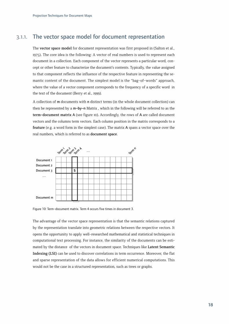
A collection of m documents with n distinct terms (in the whole document collection) can

then be represented by a m–by–n Matrix , which in the following will be referred to as the

term–document matrix A(see figure 10). Accordingly, the rows of A are called document

vectors and the columns term vectors. Each column position in the matrix corresponds to a

feature (e.g. a word form in the simplest case). The matrix A spans a vector space over the

real numbers, which is referred to as document space.

Figure10:Term–documentmatrix.Term4occursfivetimesindocument3.

The advantage of the vector space representation is that the semantic relations captured

by the representation translate into geometric relations between the respective vectors. It

opens the opportunity to apply well–researched mathematical and statistical techniques in

computational text processing. For instance, the similarity of the documents can be esti-

mated by the distance of the vectors in document space. Techniques like Latent Semantic

Indexing (LSI) can be used to discover correlations in term occurrence. Moreover, the flat

and sparse representation of the data allows for efficient numerical computations. This

would not be the case in a structured representation, such as trees or graphs.

5

Document!1

Document!2

Document!3

…

Term!1

Term!2

Term!3

Term!4 …

Term!n

Document!m


18

One basic decision in designing a vector space representation is choosing the semantics of

the columns of the vector, typically referred to as attributes or features6 . Besides word

form occurrences, more elaborate versions like stemmed word forms, lemmata or con-

cepts are typical candidates. All these techniques require linguistic preprocessing of the

data. While stemming, lemmatizing and part–of–speech tagging can be done domain–in-

dependently, the use of concepts as features requires a domain–specific ontology which is

not always available.

From a linguistic point of view, there are many characteristic features of language that are

not accounted for by the given representation.

First, the syntactical structure is completely neglected. In a simple bag–of–words repre-

sentation, “John loves Sue” and “Sue loves John” will be represented equally, despite the

obvious differences in semantics caused by different phrase structures.

Moreover, the relation between words and meaning is not a simple one–to–one map-

ping. Besides phenomena like polysemy and synonymy, context and sentence position

play a crucial role in determining the semantic content of a word token occurring in a

sentence. In the following sections, we will see how the representation can be modified to

partly account for these linguistic phenomena.

Generally, we will have to keep in mind that the vector space representation is only suited

to provide a coarse topical approximation of the semantic content of a document.

3.1.2. Reducingthedimensionality

The described techniques result in very high–dimensional document vectors. This poses

two fundamental problems: Most of the algorithms used for mapping document spaces do

not scale very well with the number of dimensions. Some of the techniques are only feasi-

ble up to a few thousand dimensions. Second, it is a mathematical fact that, since the

volume of a hypercube increases exponentially with the number of dimensions, in-

ter–vector distances tend to converge to a constant measure (Beyer et al., 1999). This makes

it harder to detect meaningful patterns. Both issues together are often referred to as the

“curse of dimensionality”.


19

6 These terms are often used interchangeably. Some authors, however, use the latter for more elabo-rate, e.g. transformed versions of the original raw data variables designated by the term “attribute”.

There are three major approaches to reduce dimensionality of the data in text processing,

which are typically combined:

• linguistic preprocessing: using linguistic knowledge to transform the original input

and filter non-informative dimensions.

• feature selection: selecting only a meaningful and useful subset of the candidate

dimensions.

• feature transformation: projecting the data into a lower–dimensional subspace.

(Tang et al., 2005).

3.1.2.1. Linguisticpreprocessing

In text processing, we possess a priori knowledge about some of the features of document

vector. For instance, words such as prepositions, conjunctions and pronouns are commonly

used merely as structural elements and thus normally contribute no topical specificity (Sa-

hami, 1998). Such words can be stored in a stop word list to remove these dimensions

from the document vector.

Further, it is an interesting fact about natural language, that in a text collection of any

size, a large part of the words appears very infrequently. Empirically, the proportion of

these infrequent words to all the words is a language–specific constant independent of

corpus size. This observation has been named “Zipf’s Law”7 . We can exploit this fact in

the feature selection step (see below.)

Additionally, stemming can be used to reduce words to a root form. For example, the

word forms “computer”, “computers” and “computing” would all be reduced to the word

stem “comput”. The classical stemming algorithm is the Porter stemmer, which utilizes

heuristic knowledge about word composition to strip suffixes off of word forms.

A more elaborate form of preprocessing is to determine the lemmata belonging to the

occurring word forms. While stemming is a heuristic process based on structural language

features, lemmatizing relies on a lexicon and thus is able to detect also irregular declina-

tions.

Many noun phrases in natural languages are actually complex constructions of multiple

word tokens — like “french fries” or “static test report”, whose meaning would be lost in

the bag–of–words approach. We can take account of this fact by integrating also mul-

ti–word terms as dimensions of a document vector. Candidates can be found by finding

frequently appearing sequences of words in the documents or providing hand–engineered

phrases for specific domains.


20

7 named after G.K. Zipf, who discovered this empirical law more than fifty years ago.

If a domain ontology is available, we can further refine our representation to produce con-

cept vectors. Of the presented representations, this is the best candidate for providing a

good approximation of the topical semantic content, since it is not the words, but their

associated concepts we are ultimately interested in. Additionally, this will not only reduce

dimensionality by resolving synonymy, but it also offers the opportunity to introduce

relations between the features based on semantic relations such as hyponymy and hy-

peronymy. Unfortunately, a domain–specific ontology is not always available and ti-

me–consuming to produce. Another typical challenge is the linguistic phenomenon of

polysemy, which refers to the fact that one word can denote different concepts in differ-

ent contexts. Probabilistic methods incorporating the context of a word form occurrence

can be used to estimate the most probable word sense (word sense disambiguation).

3.1.2.2. Featureselection

Generally speaking, the goal in feature selection is to select a subset of the original fea-

tures while maintaining as much information as possible or needed. The quality of a rep-

resentation strongly depends on the actual task, however, and there is no general agree-

ment on the best general methodology to achieve this goal. A good overview and a frame-

work for evaluating and designing different techniques is presented in (Dash, 1997). In the

area of text processing, many different selection criteria have been proposed and com-

pared empirically (Yang, 1997), (Tang et al., 2005). Among the most widely used are term

frequency thresholding, term frequency – inverse document frequency (TFIDF), and

term frequency variance, which will be discussed in the following.

Termfrequency

In term frequency thresholding, all the terms appearing less than a fixed number of

times in the whole document collection are discarded. This is often justified because these

terms will not be useful in clustering and mapping, as we are interested in words which

characterize groups of documents and are not specific to one single document. Addition-

ally, this procedure helps in de–noising the data, since typographic or orthographic errors

are likely to be in the list of least frequent words. Setting this threshold too high, however,

will result in an elimination of important dimensions. In practice, the ideal threshold de-

pends on the document collection and the computational complexity of the following

processing steps. It is normally chosen heuristically to achieve a reasonable trade–off be-

tween loss of information and computational feasibility.


21

TFIDF

Another classical criterion for feature selection is the term frequency – inverse docu-

ment frequency (TFIDF) model. Formally, it is defined as:

wheretf(i,j)denotesthefrequencyoftermiindocumentj,Nthetotalnumberofdocumentsanddf(j)thenumberofdocuments,inwhichtermjoccurs.

By introducing a penalty term inversely dependent on the document frequency, TFIDF

results in high values only for words which appear often (high tf–value), but in few docu-

ments (low df–value). Therefore, the mean TFIDF value of a term over all documents can

be used to rule out terms which are not well suited to discriminate document groups.

Varianceselection

In a similar spirit, we can use a quality measure based on the variance of the term distri-

bution across documents (Tang et al., 2005)8:

wheretf(i,j)denotesthefrequencyoftermiindocumentj,nthetotalnumberofdocuments

Again, terms which are uniformly distributed across the document collection will receive

lower values compared to more unique ones.

Remarks

Note that all of the discussed measures scale with the absolute number of occurrences,

which puts more weight onto more often occurring words, which are not necessarily the

most informative ones. This effect can be dampened by applying a logarithmic function to

the frequency values. While term frequency thresholding discards infrequent terms, TFIDF

and variance selection put a penalty on too evenly distributed terms. Hence, a combina-

tion of these techniques should result in a both more compact and informative term set.

TFIDF(i, j) = t f (i, j)! log Nd f ( j)

quality(i) =n

!j

t f (i, j)2! 1n[

n

!j

t f (i, j)]2


22

8 The proposed measure is proportional with 1/n to the variance value. This simplifies computation and is justified, since we use it only for comparison on a fixed document set.

3.1.2.3. Featuretransformation

In the recent years, a dimensionality reduction technique in text processing called Latent

Semantic Indexing (LSI)9 has received wide–spread attention. Originally designed to re-

solve the problems of polysemy and synonymy in Information Retrieval, it also estab-

lished itself as one of the classical dimensionality reduction techniques in statistical text

processing. The underlying technique from linear algebra called Singular Value Decompo-

sition (SVD) has been known and applied long before, but it was not until the 1990s that

its application to linguistic data was proposed in (Deerwester et al., 1990).

The rationale behind this technique10 is the following: Obviously, the terms in a document

are not occurring independently from each other. Rather, the topic, style and purpose of a

specific text make the occurrences of specific word groups more likely. The key idea is now

to view the production of a text as a process generating word frequencies which can be

characterized by a smaller number of underlying factors. A large document collection

(represented in the data matrix) can be used to estimate the dependencies between the

observations (word frequencies) and the underlying factors (often called hidden or latent

variables). Crucial decisions in model selection include the statistical assumptions about

data attribute dependencies (e.g. correlation or higher–order dependencies) and the nature

of the latent variables (e.g. normally distributed). Usually, a certain variability of the data

compared to the model is assumed (“noise”) – attributed to erroneous measurements, vari-

ability of word use and especially in order to favor simple, generalizable models (Occam’s

Razor).

One approach to extract latent variables is connected to the mathematical technique of

Singular Value Decomposition (SVD): Our data is given in a matrix form. Let us assume

that the number of documents m is smaller than the number of terms n. It is a mathemati-

cal fact that this matrix can be decomposed into the product of three matrices, where the

middle matrix contains a diagonal matrix with the so–called singular values in decreasing

order. The left and right matrices contains the original row and column entities as vectors

of derived orthogonal factor values (see figure 11). Therefore, we can obtain a representa-

tion of the original document space in a lower–dimensional factor space S x VT.The Matrix

Userves as “translation unit” between original and latent document space. The grey areas

in U are not used in the projection due to the corresponding zero entries in S and can

hence be omitted11.


23

9 sometimes also referred to as Latent Semantic Analysis (LSA)

10 and many other linear techniques like Principal Component Analysis, Independent Component Analysis, Factor Analysis, Projection Pursuit etc., which will partly be treated in following chapters.

11 This reduced form is often referred to as economy–sized SVD.

Figure11:TheprincipleofSingularValueDecomposition

The key features of this representation are the following: First of all, dimensionality is

reduced without a loss of information. This stems from the fact that the intrinsic dimen-

sionality of the data cannot exceed the rank of the original matrix A. Since we have less

documents than terms, the matrix A can maximally be of rank m. Consequently, a repre-

sentation in an m–dimensional space is possible and more efficient. Additionally, potential

redundancy is removed, since dependent column vectors —resulting from systematically

co–occuring words — are collapsed into one factor. This would be expressed by a zero

value for one of the singular values, indicating that one of the original dimensions does

not contribute any additional information. Further, a projection to a subspace of arbitrary

dimension k while maintaining the best fit in a squared–error sense can simply be

achieved by setting the m-k smallest singular values to zero. This does not only allow a

more efficient representation and de–noising of the data; it has also been argued that such

a lower–dimensional subspace captures the semantic relations between terms and docu-

ments in a more truthful way (Deerwester et al., 1990). Intuitively, terms that often co–oc-

cur in documents will contribute in a similar manner to the factor dimensions of the latent

space. By removing linear dependencies, redundancy and random variation, distances in

latent space are supposed to represent the semantic distance of both terms and documents

better than the original space.

Moreover, the resulting document vectors lose their original sparsity, which makes also

documents sharing few or no terms comparable in a meaningful manner. This is especially

useful in the area of Information Retrieval: if the relevance of a document for a query is

calculated by proximity in latent space (instead of the original document space), it is pos-

sible to match also documents which do not contain exactly the query terms, but closely

related terms.

LSI can thus help to resolve the issue of synonymy in this area, however, “it offers only a

partial solution to the polysemy problem” (Deerwester et al., 1990, p.21). This mainly stems

Transposed!Term–

Document!Matrix

AT!!!!!!!!!!!!!!=!!!!!!!!!!!!!!!!!!!!!!!U!!!!!!!!!!!!!!!!!!!!!!!!!!!!!!S!!!!!!!!!!!!!!!!!!!!!!VT

Singular!Values!in!

decreasing!order

Orthogonal!Matrix Orthogonal!Matrix

!1!2

!3!4

!5

0 0 0 0

0 0 0

0 0

0 0

0 0

0

0

0

0

0

0 0

0 0 0 0

0 0 0 0

0 0 0 0

0 0 0 0

0

0

0

0


24

from the fact that each term is represented as a single point in the projected term space,

which makes it inherently impossible to adequately account for multiple word meanings.

Recently, the presented LSI technique has been criticized for its weak statistical founda-

tion. A statistically more well–founded approach to LSI is presented in (Hofmann, 1999).

Other preprocessing techniques for extracting features from the original data are Principal

Component Analysis (PCA), which is essentially a Singular Value Decomposition on the

covariance matrix of the data and Independent Component Analysis (ICA), which can be

used to detect higher–order statistical dependencies between the attributes. These will be

treated more in depth in section 3.3.

3.2. Similaritymeasures

The choice of a similarity measure is crucial for the mapping process. It needs to fit the

user’s subjective expectations about similarity of documents. But it also has to be comput-

able efficiently from the given representation, as it will intensively be used in further

processing. As the data is represented in a vector space, the similarity measure will be

computed on basis on distance relations. The most popular in text processing are euclid-

ean, Mahalanobis and cosine distance.

3.2.1. Euclideandistance

The euclidean distance is the most intuitive distance measure, as it is commonly used to

evaluate distances in two– or three–dimensional space. It is defined as:

In fact, it is only a special case (p=2) of the general Minkowski metric :

The euclidean distance is invariant with respect to rotating and translating the data, how-

ever, not to scaling the data. One potential problem with this metric for text data is the

fact that the largest scale features dominate the others, which introduces an importance

weighting among the variables “through the back door”. For use in text processing, nor-

malizing the document vectors to unit length is advisable when using this measure, other-

wise, long documents will tend to be much further apart than short documents — inde-

pendent of the semantic content — which is normally not desired. Further and independ-

deuclidean(x1,x2) =!

!k

(xk1! xk

2)2

dminkowskip(x1,x2) = (!k!xk

1" xk2!p)

1p


25

ent of normalization, statistical dependency among the variables may also distort dis-

tances. (Jain et al., 1999)

3.2.2. Mahalanobisdistance

This latter factor is accounted for —at least for correlations—in the squared Mahalanobis

distance by weighting the attributes based on the covariance of the data:

where! denotesthecovariancematrixofthedata.

This distance metric requires the calculation and inversion of the complete covariance ma-

trix, which can become fairly large for high–dimensional data, as its size grows quadrati-

cally with the number of dimensions. If the data is pre–processed with PCA or a related

technique to decorrelate the dimensions, the euclidean distance can be used instead. This

is usually the more practical solution.

3.2.3. Cosinesimilarity

Geometrically speaking, the cosine similarity corresponds to the angle between the docu-

ment vectors. It does not depend on the length of the corresponding vectors. If both

documents vectors have unit length, it is equivalent to the dot product. Its values range

from - 1 to 1, where the latter denotes maximum similarity (which happens if and only if

the two compared vectors are equivalent), a zero value shows that the two vectors are

orthogonal, and a value of –1 indicates that the two vectors are exactly opposed. A trans-

lation to distance is fairly trivial due to the existence of these bounds.

3.2.4. Normalization

The choice of a suitable distance measure is closely connected to the normalization of the

document vectors. Typical combinations include

dmahalanobis(x1,x2) = (x1! x2)!!1(x1! x2)T

dcosine(x1,x2) =< x1,x2 >

!x1!!x2!


26

• Normalizing document vectors to unit length and using euclidean distance or cosine

similarity (which can then be computed very efficiently by calculating the dot prod-

uct)

• Normalizing term vector variances to one and using Mahalanobis distances. How-

ever, this requires the calculation and storage of the covariance matrix of the fea-

tures.

• Applying SVD or PCA to project to a lower–dimensional dimensional subspace with

uncorrelated features. The distances can then be calculated more efficiently using

the euclidean or cosine measures, and at the same time, the possible distortion intro-

duced via correlated axes is not a problem. Again, in the projected space, document

vector length can be normalized to unity in order to eliminate effects based on

document length and to facilitate calculations.

3.3. Projectiontechniques

The calculation of a document map can be seen as an optimization problem. Given a for-

mal representation of the quality of a certain coordinate configuration (the error or stress

function), the task is minimize this function, resulting in the best possible map according

to this criterion.

We can distinguish two different methodologies in achieving this goal:

• Techniques like PCA, ICA and Isomap use an algebraic approach to solve the minimi-

zation problem. This puts some constraints on the class of computationally feasible

error functions, but allows the one–shot calculation of an explicit projection func-

tion.

• Neural methods (like MDS and its variants) start with an initial configuration, which

is gradually modified according to a heuristics until a stopping criterion is met. These

algorithms can in principle optimize any differentiable error function. However, de-

pending on the initial configuration, only a local optimum might be found. The map-

ping from input to output space is calculatedly only implicitly. Many variants exist,

differing in error functions and optimization approaches.

Another important distinction can be made with respect to the capabilitites of the algo-

rithms:

• Linear methods like PCA can only apply a linear mapping to the data. Metaphorically

speaking, the projection plane can be turned, scaled and skewed in document space,

however, it will always remains “rigid”.

• Non–linear methods techniques allow — to stay with the metaphor — “elastic”

maps which can lie folded, twisted or locally distorted in document space and are

then unwrapped onto a plain cartesian map for display purposes.


27

3.3.1. PrincipalComponentAnalysis(PCA)

Principal Component Analysis (PCA)12 is an application of the above mentioned Singular

Value Decomposition techniques. The aim of the projection is to find k orthogonal axes

such that the greatest variance of the data is preserved. It can be shown that solving this

optimization problem also minimizes the projection error in a squared–error sense.

Therefore, the proposed technique can not only be used to decorrelate and compress data

in the preprocessing steps, but also to project the data into a two–dimensional cartesian

space for cartographic displays.

A general algorithm for calculating the k–dimensional approximation of the data points

given in a data matrix can be found in (Himberg, 2004) and (Duda et al., 2000). Essentially,

it is based on an eigenvector decomposition of the covariance matrix. Many efficient im-

plementations exist due to the popularity and generality of the approach.

The algorithm scales well with the number of data instances, however large dimensionality

of the data set might result in long computation times and high memory demands: For n

feature dimensions, it requires O(n2)memory for the covariance matrix, and a time in

O(kn2) for finding the k leading eigenvectors (Karypis & Han, 2000).

For two–dimensional document space projections, the method has the advantage that it is

well analysed and mathematically well–founded. Based on algebraic techniques, the opti-

mal solution can be calculated in one run and does not require training or additional pa-

rameters like iterative neural network techniques. Of practical relevance can be the fact

that the principal coordinates might be available from preprocessing already, in which case

no additional computations are necessary to display the map.

Figure12:Exampledatasets.Directionof maximumvarianceisindicatedby thearrow.

However, it has to be noted that the assumption that the directions of maximum variance

are in turn also the most interesting axes is not necessarily true. Figure 12 (left) shows a

dataset where the direction of maximum variance is well–suited to capture the cluster

structure of the data. However, in the example on the right side, the direction of maximum


28

12 Sometimes PCA is also referred to as Karhunen–Loeve transform or Hotelling transform.

variance is exactly orthogonal to the axes which would be most useful to distinguish the

two clusters.

Some more remarks: PCA optimizes a squared–error criterion on euclidean distances. This

will put much weight on large distances in the data. It is a reasonable assumption that for

most document mapping applications inner–cluster structure and local neighborhoods are

at least as important as preserving global distances. Further, the linear nature of the pro-

jection based on the covariance data possibly fails to capture non–linear dependencies in

the data. In fact, the dimension reduction will only be fully successful, if the manifold

spanned by the data points is a hyperplane.

AnoteonIndependentComponentAnalysis(ICA)

This last point could in principle be adressed by using Independent Component Analysis

(ICA). This technique from multivariate data analysis extracts maximally independent

components. Unlike in PCA, the statistical independence is not only evaluated with re-

spect to correlation data (i.e. linear dependence), but also higher–order statistical depend-

encies are taken into account. Originally used for blind signal separation, like separating

different overlayed voices in audio recordings (Hyvärinen & Oja, 2000), it has also been

shown to be a fruitful approach for linguistic feature extraction (Honkela&Hyvärinen,

2004) and even superior to LSI/PCA in text data feature extraction in some studies (Tang

et al., 2005).

However, ICA suffers from two ambiguities (Hyvärinen & Oja, 2000): Neither the scales

and signs of the independent components nor the order (or importance) of the independ-

ent components can be estimated. Especially the latter point is problematic in visualiza-

tion, as in principle any combination of two independent components might be a candi-

date for constituting the axes on a map display. For this reason, it will not be considered

further in this thesis.

3.3.2. Multi–DimensionalScaling(MDS)

The term Multi–Dimensional Scaling (abbr. MDS) covers a whole class of data analysis

techniques. The general aim is the following: Given a matrix of inter–object dissimilarities

D and a target dimension k, find a configuration of points in the target space, such that

inter–point distances correspond the original inter–object dissimilarities as good as possi-

ble. The quality of a target space configuration is measured by an error or stress function.

MDS techniques vary both with respect to the stress function and the techniques used to

minimize the stress. (De Backer et al., 1998)


29

MDSAlgorithm

A general algorithm for MDS typically involves the following steps (De Backer et al., 1998),

(Manly, 1994):

Given is a dissimilarity matrix D and target dimension k.

1. Compute a starting configuration X0with dimensionality k. It can be chosen ran-

domly or according to some heuristic estimate of a promising candidate, such as a 2D–

projection by principal component analysis.

At iteration t:

2. Compute the distances dij for the current configuration Xt

3. Compute the target distances d*ij. The distance between target distance and con-

figuration distance is called disparity and quantifies the misplacement of an item.

4. Compute the stress function value and gradient13 for the configuration. The stress

function quantifies the overall misplacement in the current coordinate configuration

based on the disparities.

5. Adjust the coordinates of the configuration according to the gradient of the stress

function and the learning rate.

6. Stop if the algorithm has converged, otherwise go to step 2.

MDSvariants

MDS techniques can differ in many aspects. One of them is the interpretation of the given

dissimilarities, which affects the disparity calculation in step 3 of the presented algorithm.

• In classical MDS, the dissimilarities are assumed to be a distance matrix and the

lower–dimensional approximation is evaluated with a squared–error calculation. In

this case, the solution could also be found – analogously to the SVD and PCA tech-

niques presented above – by solving an eigenvector problem. In fact, if the distances

D are euclidean, a classical MDS and PCA will essentially deliver the same result

(Everitt and Dunn, 2001).

• An MDS is called metric in the more general case of a linear or polynomial relation

between configuration distances and original dissimilarities. If, e.g., a linear rela-

tionship between target distance and original dissimilarity is assumed, the disparities

can be calculated with d*ij= a+bdij+e , where e is an error term and a and b are


30

13 The gradient is a vector calculated from the partial derivatives with respect to all degrees of free-dom of the error function. It is used to estimate how the projected coordinates have to be adjusted in order to reduce the stress in the current configuration.

constants. Values for these parameters are estimated by calculating a linear regres-

sion based on the current configuration and the given distances. After that, the

actual disparities can be calculated (Everitt and Dunn, 2001).

• If this precondition is not fulfilled, but the relation is any other monotonic function,

the MDS is called non–metric MDS (Manly, 1994). In this case, only the rank order

of the items is to be approximated in the projection and not the exact values. The

disparities are obtained from a monotone regression in order to make the disparities

match the rank order of the original dissimilarities while keeping them as close as

possible to the configuration distance values.

MDSStressfunctions

Besides the choice of a learning rate function and a stopping criterion, the most important

design decision is the choice of a suitable stress function.

Generally, it has the following shape (Himberg, 2004):

whereN(D)denotesanormalizationfunctionandF(dij,λt)denotesaweightingfunctiondependent

ontheoriginaldissimilarityandpossiblyaniteration–dependentdecayfactorλt.

The normalization function N(D) has no effect on minimization as such, but is used to

make stress values comparable across data sets. To ensure that uniform scaling of the dis-

similarities does not affect the stress measure A, a reasonable choice would be

Different weighting functions F(dij,λt)for the squared error term result in different

mappings:

• By setting F=1, we obtain raw stress. This is the measure used in classical scaling,

which will lead to solutions very similar to PCA. An important property is that long–

range distances have a larger effect on stress values, which is sometimes not desir-

able.

• Setting F(dij)=1/dij yields the widely used Sammon mapping. By decreasing stress

caused by originally large dissimilarities, the local neighborhood of items is empha-

sized. This typically results in a better local representation and less overlapping data

points.

Egeneric = N(D)N

!i< j

(di j!d"i j)2F(di j,"t)

N(D) =1

!Ni< j d2

i j


31

Another possibility to reduce the influence of large dissimilarities — in order to improve

local topology preservation — is the logarithmical transformation used in maximum

likelihood MDS:

3.3.3. MDS–relatedtechniques

Over the last years, a multitude of variations of the above presented MDS techniques has

been developed, some of which will be discussed in the following.

3.3.3.1. Springembedding

One approach that shares many properties with the MDS technique is the so–called spring

embedding. First presented in the BEAD system (Chalmers&Chiton, 1992), it is motivated

by a physical model: Documents are represented as particles in 2D– or 3D–space. These are

subject to a repulsive force decaying linearly with particle distance and to an attractive

force which is proportional to the original inter–document similarity. The particles can

hence be thought of as being connected by damped springs. For stability, a friction force

increasing with particle speed is usually introduced. By approximating the force impact of

more distant particles with the help of virtual meta–particles, the otherwise quadratic time

complexity can be reduced to O(nlogn).

The major differences to classical scaling are the use of a linear (instead of quadratic)

stress function and the fact that each particle has its own momentum. This may help

avoiding local minima, but on the other hand lead to unstable configurations and thus to

longer convergence times. A similar behavior can be achieved in MDS by using a gradient

descent algorithm which has a different momentum factor for each gradient dimension like

SuperSAB (Tollenaere, 1990).

3.3.3.2. CurvilinearComponentAnalysis(CCA)

Curvilinear Component Analysis (CCA) introduces a new stress function as well (De-

martines & Herault, 1997): The weighting function F is bounded and monotonically de-

creasing with the projected distances d* (and not with the original dissimilarities as in

E = N(D)N

!i< j

(log(di j)! log(d"i j))2


32

the cases before). This induces a SOM–like topology preservation and is claimed to im-

prove performance in unfolding complex structures. Frequently used are Gaussian bell

functions. Additionally, the width of the Gaussian can decreased over the iterations, which

makes larger distances less influential over time. This results in a rough layout of the map

in the first iterations, which is locally optimized later in the process. Again, this adds flexi-

bility, but in turn makes the target function of optimization more complex.

3.3.3.3. Isomap&CurvilinearDistanceAnalysis(CDA)

Two related refinements of the MDS — Isomap and Curvilinear Distance Analysis (CDA)—

introduce a new distance measure on the data points.

Both techniques share the same key idea: Instead of relying on euclidean distance, which

makes the unfolding of complex non–linear structures like a spiral impossible (Figure left),

pairwise point distances are estimated as to reflect the geodesic distance (i.e. the distance

along the space spanned by the data points; see Figure 13, center). Typically, the geodesic

distance is approximated by the shortest nearest neighbor path on some randomly selected

landmark vectors (see Figure 13, right). Improvements can be achieved with a Vector

Quantization step in order to place the landmark vectors well distributed with respect to

the input data density.

Figure13:Approximatinggeodesicdistancewithlandmarkvectors(modifieddrawingbasedonLee,2003).

The major difference between the two techniques is the optimization algorithm: Isomap

uses an eigenvector decomposition on the computed geodesic distance data to calculate

the projection (similar to PCA), while CDA applies a stochastic gradient descent as pre-

sented before in the MDS algorithm.

For a good theoretical and empirical comparison of these two techniques see (Lee et al.,

2003).

J.A. Lee et al. / Neurocomputing 57 (2004) 49–76 51

(a) (b) (c)

Fig. 1. Distance between two points: (a) two points on a manifold with a spiral shape, (b) the Euclideandistance between them in the data space, (c) the distance along the manifold, which is the one approximatedby the curvilinear or geodesic distance.

Nonlinear methods not su!ering from this disadvantage are nonlinear variants ofthe metric MDS, like Sammon’s nonlinear mapping (NLM) [18] or the CurvilinearComponent Analysis (CCA) [3,8]. These algorithms minimize criterions which com-pletely di!er from the one used by PCA. They are based on notions like topologyand neighborhood. Actually, they build a mapping in such a way that the pairwisedistances between the raw data vectors are reproduced between the mapped vectors.These algorithms show good capabilities for the unfolding of nonlinear manifolds. Theirlimitations come from the distortions that can exist between the distances measured inthe data space and the distances measured in the manifold space (see the example ofthe spiral in Fig. 1). The last evolutions of the distance-preserving techniques avoidpartly the problem by using a more complex metric than the Euclidean distance. Forexample, the Curvilinear Distances Analysis (CDA) [15,16] and Isomap [20], devel-oped independently and compared in this paper, compute a ‘curvilinear’ or ‘geodesic’distance [2]. This metric can measure good approximations of the distances along themanifold, without shortcuts as does the Euclidean distance (Figs. 1b and c). By theway, it is worth to notice that the geodesic distance could be used not only in MDSand CCA, but also in Sammon’s NLM. However, such a combination has apparentlynot been published yet and is not investigated here.The remainder of this document is organized as follows. Section 2 explains and

de"nes the curvilinear (or geodesic) distance. Sections 3 and 4, respectively, detailhow Isomap and CDA works. In order to compare both algorithms, Section 5 showssome experimental results and Section 6 discusses them. Finally, Section 7 draws theconclusions and sketches some perspectives for future work.

2. Curvilinear distance

At the "rst glance, the curvilinear distance appears as a very strange concept. Indeed,although it is directly apparented with the Euclidean distance, the curvilinear distancedepends not only on the two points between which the distance is measured, but alsoon other surrounding points. This use of more than two points is totally unknownin the world of Lp norms, where e.g. Euclidean and Manhattan distances are comingfrom. A well-known exception is the Mahalannobis distance, for which the covariance

J.A. Lee et al. / Neurocomputing 57 (2004) 49–76 51

(a) (b) (c)

Fig. 1. Distance between two points: (a) two points on a manifold with a spiral shape, (b) the Euclideandistance between them in the data space, (c) the distance along the manifold, which is the one approximatedby the curvilinear or geodesic distance.

Nonlinear methods not su!ering from this disadvantage are nonlinear variants ofthe metric MDS, like Sammon’s nonlinear mapping (NLM) [18] or the CurvilinearComponent Analysis (CCA) [3,8]. These algorithms minimize criterions which com-pletely di!er from the one used by PCA. They are based on notions like topologyand neighborhood. Actually, they build a mapping in such a way that the pairwisedistances between the raw data vectors are reproduced between the mapped vectors.These algorithms show good capabilities for the unfolding of nonlinear manifolds. Theirlimitations come from the distortions that can exist between the distances measured inthe data space and the distances measured in the manifold space (see the example ofthe spiral in Fig. 1). The last evolutions of the distance-preserving techniques avoidpartly the problem by using a more complex metric than the Euclidean distance. Forexample, the Curvilinear Distances Analysis (CDA) [15,16] and Isomap [20], devel-oped independently and compared in this paper, compute a ‘curvilinear’ or ‘geodesic’distance [2]. This metric can measure good approximations of the distances along themanifold, without shortcuts as does the Euclidean distance (Figs. 1b and c). By theway, it is worth to notice that the geodesic distance could be used not only in MDSand CCA, but also in Sammon’s NLM. However, such a combination has apparentlynot been published yet and is not investigated here.The remainder of this document is organized as follows. Section 2 explains and

de"nes the curvilinear (or geodesic) distance. Sections 3 and 4, respectively, detailhow Isomap and CDA works. In order to compare both algorithms, Section 5 showssome experimental results and Section 6 discusses them. Finally, Section 7 draws theconclusions and sketches some perspectives for future work.

2. Curvilinear distance

At the "rst glance, the curvilinear distance appears as a very strange concept. Indeed,although it is directly apparented with the Euclidean distance, the curvilinear distancedepends not only on the two points between which the distance is measured, but alsoon other surrounding points. This use of more than two points is totally unknownin the world of Lp norms, where e.g. Euclidean and Manhattan distances are comingfrom. A well-known exception is the Mahalannobis distance, for which the covariance


33

3.3.3.4. RelationalPerspectiveMap(RPM)

The Relational Perspective Map introduced in (Li, 2004) adds another interesting twist to

traditional MDS techniques: Topological constraints on the target space are introduced.

Stress optimization is e.g. computed on a torus or sphere surface instead of an uncon-

strained, infinite cartesian plane. After optimization, the surface is “unwrapped” and pre-

sented in the usual two–dimensional cartesian plane (see Figure 14).

Figure14:TheRPMprinciple(Li,2004)

Again, this modification affects primarily the distance measure, since there are now sev-

eral ways to connect two points with a straight line in image space. The technique allows

the use of repulsive force, since projection items cannot escape the finite surface. A posi-

tive feature of the RPM is the fact that map degeneration close to the borders — which is

a notorious problem in mapping — vanishes. However, care has to be taken in map pres-

entation to communicate the actual closeness of seemingly very distant items, like points

located on the very left and very right of the map. Additionally, the map does not have a

center and a periphery anymore, which is useful only if the dataset tends to be distributed

evenly on a sphere–like surface, which is usually not the case for text data.

3.4. Discussion

Clearly, all of the presented techniques have their advantages and disadvantages. The

optimal choice in a specific scenario depends not only on the available data, but also on

conceptual decisions concerning the usage of the produced maps and computational limi-

tations. In order to facilitate these design decisions, some of the characteristics of the

presented techniques will be summed up comparatively in the following.

Capabilities

In PCA, only linear projections are possible. Moreover, a large portion of the available data

is discarded. The first two eigenvalues typically do not cover even half of the overall vari-

The starting point of the RPM algorithm is a set ofabstract data points si, i!1, y, N with a distance matrixdij, i,j!1, y, N. The RPM algorithm maps data points siinto image points ti in a 2-D space in such a way thatvisual distances between the image points, denoted by dij,resemble the distances dij. The image points ti, i! , y, Ntherefore provide a 2-D visualization of distance informa-tion of the initial dataset. For the sake of our discussion,we call dij and dij, respectively, relational and image distancematrices.As illustrated in Figure 1, the RPM algorithm first maps

data points onto the surface of a torus, then the flatrectangle by a vertical and a horizontal cut. The secondstep is more or less straightforward, thus the RPMalgorithm focuses on how to map the dataset onto thetorus surface so that the configuration of the imagepoints reflects the distances information in the originaldataset.In order to find an appropriate configuration, the RPM

algorithm considers the image points together with thetorus as a force-directed multiparticle system: the imagepoints are considered as particles that can move freely onthe surface of the torus, but can not escape the surface.The particles exert repulsive forces on each other so that,guided by the forces, the particles rearrange themselves toa configuration that visualizes the relational distances dij.In particular, the RPM algorithm uses Eq. (1) as the

total potential energy to characterize a configuration.

Ep :!X

ioj

dijpdpij

with E0 :! "X

ioj

dij ln#dij$: #1$

The parameter p in Eq. (1) is called the rigidity whosevalue is a real number between "1.0 and +N. Followingthe usual physical formalism, the forces between theparticles are characterized by

fij :!qEp

qdij! "

dijdp%1ij

: #2$

From a physical point of view, the RPM algorithmsimulates the multiparticle system described above byallowing the particles to move along the repulsive forcesand therefore minimizes the potential energy. Eq. (2)states that the repulsive force between two image pointsis proportional to their relational distance, therefore data

points with a larger relational distance between them willbe mapped to further apart positions on the torus surface.Assuming p!0, Eq. (2) also states that the repulsive forcebetween two image points is reversely proportional to theimage distance between them. This means that moreclosely located image points have larger contribution tothe total potential energy and therefore carry moreinformation about the original dataset. In general, theparameter p provides a means to control how fast therepulsive force decreases with increasing image distances,and therefore controls how strong the system biasestowards information represented by closely located imagepoints.

Related worksIn a broad sense, the RPM method can be considered as atechnique of multidimensional scaling (MDS1,2) that, as afamily of techniques, aims to produce multidimensionalgeometric representation of data. RPM resembles con-ventional MDS in problem setting, but differs inapproach. To put it in a simplified way, compared tothe energy function Eq. (1) used in this study, the usualMDS tries to minimize the so-called stress function asdescribed in below

E !X

ioj

#dij " dij$2: #3$

By minimizing Eq. (3), the MDS algorithm forces imagedistance dij to approach the relational distance dij, whichis also called dissimilarity or proximity in traditionalMDS literatures.When we consider the optimization process of MDS as

a force-directed dynamic system, the image points exerttwo kinds of forces on each other depending on theimage and relation distances: the attractive force whenthe image distance is larger than the relational distance;or the repulsive force when the image distance is smallerthan the relational distances. In contrast to this kind ofdual force system, the RPMmodel only employs repulsiveforce but resorts to topological means (closed surface) toprevent the system from degeneracy.A well-known problem of conversional MDS is that the

stress function aggregates uniformly over all distances sothat the long-range relational distances often dominate

Dataset with 4 points inhigh dimensional space

4 image points on the torus surface

RPM map of thedataset

Figure 1 Model of the RPM method.

Relational perspective map J. Xinzhi Li

50

Information Visualization


34

ance of the data set. This means that most of the available information is not displayed.

Especially directions which are only locally important will be neglected, which typically

leads to a high number of almost overlapping data points.

The greater power of non–linear mapping allows the unfolding of very complex topologies

in MDS techniques. By adjusting the F–function, a good combination of local truthfulness

of the projection and improved readability of the map — by reducing overlap between

close items — can be achieved. It has been shown that with respect to preserving topology

in small neighborhoods, Sammon’s mapping and especially CCA are superior to PCA (Him-

berg, 2004).

Optimizationalgorithm

Neural methods find the best solution iteratively by gradient descent. This may result in

sub–optimal solutions due to local minima of the stress function; furthermore, it produces

additional learning parameters which have to be adjusted manually. Different starting lo-

cations may result in different maps, which makes consistent initialization an issue.

Moreover, an explicit projection function is not available after training.

The presented algebraic methods do not depend on initialization and determine the opti-

mal solution one–shot. Additionally, the projection function is explicitly available in ma-

trix form.

Semanticsoftheprojectionaxes

In MDS, only the inter–object distances and not their original locations are used in the

calculations, it is obvious that different projections can minimize the stress criterion

equivalently. For instance, any rigid transformation of a configuration will yield the same

stress value. The semantics of the projection space is defined by the spatial relations of the

projected items, and not their absolute positions.

In algebraic methods, the two axes of the projection space represent the values of the two

dominant factors in the data. This means not only that on–map distances are more consis-

tently related to inter–document distances 14 , but makes it in principle possible to deter-

mine labels for the axes or “blank spots” on the map. However, it has to be noted that the

axes are typically a linear combination of very many of the original features; conse-

quently, they do typically not correspond to concepts easily graspable or expressible in

natural language.


35

14 If we ignore the projection error, there is a linear relationship between original distance and pro-jected distances for any two points on the map. Moreover, the projection error should be more uni-formly distributed across the map than in non–linear mapping.

Performanceandcomplexity

The runtime of the MDS algorithm scales linearly with the number of dimensions and

quadratically with the number of projected items. This makes MDS a feasible solution for

high–dimensional representation and a controlled number of instances, which is a typical

situation in Information Retrieval. However, very large document collections will result in

inacceptable computation times. Significant performance improvements can be achieved

by gradually narrowing the stress influence to local neighborhoods as used in CCA.

We encounter the reverse situation in the algebraic methods: as the algorithm works on a

singular value decomposition of the data covariance matrix, its space and time complexity

is quadratic with the number of dimensions (rather than the number of documents).

3.5. Empiricalresults

It is interesting to see the effects of the discussed theoretical properties in practice.

In order to create some test projections, a test set of 57 freely available printer documents

was pre–processed by lemmatizing the contained words, discarding lemmata which oc-

curred less than 5 times in all documents together and selecting the 3000 dimensions with

the highest variance values. After that, values were weighted both according to font size

and IDF value. A PCA dimension reduction on the centered data with a variance threshold

0f 0.0001 yielded 57 remaining latent dimensions. The first two principal components had a

variance of 13.9% and 13,4% of the summed principal component variance, thus capturing

together 27,3% of the total variance. Mutual dissimilarities in latent space were computed

with the euclidean distance measure. On this basis, CCA and Sammon’s map were com-

puted; both were initialized with the first two PCA coordinates in order to achieve quicker

convergence and maintain comparability of the maps.

The resulting maps are plotted in figure 15. Several observations can be made:

• In the PCA projection, many points are almost co–located, resulting in compact

clusters with much whitespace in between. This loss in local topology results from

the emphasis put on large distances and the globality of the projection. In the fol-

lowing section, we will see that occasionally even very distant documents are be

presented close together due to the neglect of a huge part of the available data.

• CCA and Sammon’s map result in “blown up” clusters with more evenly distributed

documents. From the visualization perspective, the available map space is used more

efficiently, since clusters of similar documents will occupy more space than in a lin-

ear projection. In the Sammon’s map, most cluster boundaries remain intact; in the

CCA projection, clusters are not clearly distinguishable. On the other hand, Sam-

mon’s map tends to produce round structures with lower average distance towards


36


37

Figure15:Projectionsofatestsetof57printermanuals.Colorsmarkk–meansclusters(k=5).

Sammons Map

PCA

CCA

the edges, while CCA produces a well–distributed map. Care has to be taken in visu-

alization, however, to communicate the non–linear relationship of map–distance and

similarity. In extreme cases, cluster borders can get so close together that users might

read high similarity between actually very dissimilar objects out of the map.

• The cluster marked with the green ‘+’–symbol is located in the middle of the PCA

plot. This indicates average values in both PCA components, which hints at a bad

distinguishability from the rest of the documents. Consequently, in both CCA and

Sammon’s map, the cluster is torn apart and spread across the map. This situation is

problematic as it might lead to wrong conclusions. On the other hand, also in the

PCA plot it is counterintuitive that the least distinguishable documents are located in

the center. Only knowledge about the nature of PCA projection on side of the user

can lead to the right interpretation, which cannot be pre–supposed.

Projectionquality

These points are closely to connected to the quality evaluation of the computed coordi-

nates. However, comparing the presented algorithms and their output is notoriously diffi-

cult, as each of the presented techniques highlights different aspects of the data.

One possibility for a coarse graphical inspection is to create a biplot of the original dis-

similarities and the projected distances (see figure 16). For an ideal mapping, the data

points line should form a straight line through the origin. Data points located, e.g. in the

lower right corner of the plots indicate distances which are originally large, yet small in the

projection, thus leading to a false indication of neighborhood relations. We can observe

that there are significantly more of these points in the PCA plot, which hints at a low

truthfulness of the projection for the involved documents. The CCA and Sammon’s map

plots do not exhibit dramatic differences, with a slight advantage for the Sammon’s map as

more points accumulate in the upper right.

Figure16:Biplotsoforiginal vs.projecteddistances

One option to quantify the mentioned “false neighborhood mistakes” to compare projec-

tion techniques would be the trustworthiness measure. Essentially, it is computed by

0 0.5 1 1.50

0.2

0.4

0.6

0.8

1

1.2

1.4

Original Distances

PC

A

0 0.5 1 1.50

0.2

0.4

0.6

0.8

1

1.2

1.4

Original Distances

CC

A

0 0.5 1 1.50

0.2

0.4

0.6

0.8

1

1.2

1.4

Original Distances

SA

M


38

comparing the rank orders of projected and original distances in a neighborhood of certain

size with respect to each projected item. For details about the measure, see (Himberg,

2004, p.31).

Summary

The test confirmed the theoretical differences between the linear PCA projection and the

non–linear MDS techniques Sammon’s map and CCA. PCA has its strengths in feature

extraction and data pre–processing, but should be used with caution for map displays.

Based on the given data, the rather novel CCA technique seems to be slightly superior to

the traditional Sammon’s mapping due to its better run–time and efficient map space us-

age. However, further tests would have to be conducted to verify this impression.


39

4. Synthesis:Fromcoordinatestomaps

Clearly, the presented techniques do not result in maps ready for use. Point–displays alone

— without further information or interaction possibilities — will not be very useful due to

the high amount of extra cognitive load necessary to interpret the results.

In section 4.1, some common methods to create meaningful maps out of the computed

coordinate information will be discussed. Principles for map interaction are presented in

section 4.2. Since these topics would easily exceed another thesis, only an overview of the

key issues and possible solutions will be given.

Some of the presented techniques have been implemented and compared in the ASADO

system, which was designed and produced in the context of the study project ASADO at

Universities of Osnabrück and Hildesheim in cooperation with the aircraft manufacturer

AIRBUS. Some of its key features are presented in section 4.3.

Section 4.4 closes this work with a discussion of open questions and challenges for future

research.

4.1. Cartographictechniques

Although limited and well–defined set of graphical properties is available to communicate

the available information, the possibilities of their usage and combination are endless . The

groundwork towards a systematic treatment of visual language and its grammar was

laid by Jacques Bertin in his famous “Semiology of Graphics” (Bertin, 1984). He distin-

guishes marks (points, lines and areas), positional, temporal and retinal (color, size, shape,

saturation, texture and orientation) graphical variables.

Obviously, the invariant metaphor across the presented document approaches is the pres-

entation of documents as point–like marks as to encode their similarity as proximity.

These marks can possess various retinal attributes to convey additional information, like

document meta–data or relevance with respect to a query. An appropriate encoding has to

be carefully chosen in order to avoid a mismatch between expressiveness of a graphical


40

variable and the displayed data type. If e.g. color is used for a large number of unordered

nominal values, viewers might infer that similar colors denote similar classes — an over-

interpretation induced by the use of a too expressive visual variable. On the other hand,

an attribute might also be not expressive enough to represent the available information —

for instance, shape encoding is usually considered ill–suited for quantitative data due to its

intrinsically discrete nature. Typical encodings include icons (shape) for nominal values

like the document type, and color, brightness, opacity or size to display query relevance.

Not only the document markers can carry information; frequently, the map area itself

serves to communicate properties of the dataset. The possibilities are numerous: Clusters

might be marked by a textured or colored background area. Nearest document neighbors

can be linked with a line. If a non–linear transform was used to calculate the coordinates, a

relief–like structure can be used to indicate the degree of local space transformation. In

this case, either a color scale or isolines are typically used to create an impression of depth

(see figure 16).

Figure16:Cartia’sThemescape.Colorandisolinesareusedtocreateadepthimpression.15

Another important factor is labeling. Documents, document groups and map areas can be

supplied with a text label to facilitate quick overview and orientation. This is possibly the

biggest challenge in automated map creation, since unambiguous label placement without

creating overlap and visual clutter is already very hard to do by hand. Often, labels are

supplied on interaction, such as on mouse click or rollover.

Concerning map area marking and labeling, the establishment of visual hierarchies is a

crucial factor (see figure 17). Some information is supposed to be perceived immediately in

order to provide quick overview, other information gains importance once a salient map


41

15 retrieved from http://transcriptions.english.ucsb.edu/archive/colloquia/Kirshenbaum/ATT00163.HTM

region has been identified. Additionally, if several attributes have been encoded in differ-

ent retinal coordinates, none of these should be so dominant that it cannot be ignored, if

the user is interested in other attribute values.

Figure17:Establishingvisualhierarchiesbyfontsizeandcolor(Skupin,2002)

4.2. Mapinteraction

Many of the above mentioned challenges can be met by introducing interactive features.

One of the classical paradigms for interactive information visualization, which is especially

well–suited for map interaction, is Ben Shneiderman’s

“[…] Visual Information Seeking Mantra: Overview first, zoom and filter, then

details–on–demand” (Shneiderman, 1996, p.3)

These four tasks constitute the fundamental interaction facilities users expect from an

interactive map:

• Overview: A zoomed out, coarse view of each variable is presented in the beginning

to support quick orientation.

• Zoom: Once a region of interest has been identified, users typically want to examine

it closer. Both a linear magnification or a non–linear fisheye distortion are popular.

Smooth zooming improves keeping a sense of position and context.

• Filter: The user should be enabled to hide or disable uninteresting items. The filter-

ing is often based on additional, not yet encoded variables. A rapid display update is

the goal in order to indicate the effects of an action immediately.

• Details–on–demand: For a set of selected items, additional information should be

made available on request. Usually this is achieved via popup windows, tooltips on

mouse rollover or a separate details panel with a fixed position.


42

Further, some supplementary, secondary tasks can be identified:

• Relate: Enable the user to view relationships between items or compare items.

• History: Keep a history of user actions in order to support undo, replay and pro-

gressive refinement.

• Extract: Allow the extraction of sub–collections and corresponding query and filter

parameters for later re–use.

Additionally, if multiple views are provided at the same time, linking and brushing is the

predominant technique to connect items across visualizations. A selection in one view will

mark the selected items in all other views, thus allowing comparison among views and to

easily combine the advantages of each offered visualization type.

4.3. TheASADOsystem

Some of the presented projection techniques and the above mentioned interaction princi-

ples have been implemented prototypically in the ASADO system. It was developed as part

of the study project ASADO at the Universities of Osnabrück and Hildesheim in coopera-

tion with the aircraft manufacturer AIRBUS. A demo version of the system is available at

http://der-mo.net/ASADO.

Figure18:Screenshotof theASADOsystem.


43

On the basis of a fixed document collection, a map projection is computed and displayed.

(see figure 18) As the analysis of chapter 2 revealed, PCA is best for coarse cluster struc-

ture inspection, while CCA and Sammon’s Map preserve local topology better. Accordingly,

both sets of coordinates are computed and the displayed coordinates are a linear mixture

of these two coordinate components.

The relative contribution of the two coordinate components can be adjusted by the user

with a slider control (see figure 19). This allows the user to blow up and shrink the clusters

according to their needs.

Cluster are marked by cloud backgrounds. On rollover, automatically computed keywords

are displayed to characterize the cluster contents. Single document items reveal their title

as a tooltip on rollover (see figure 20).

Figure19:Slidecontrolforcoordinatemixture.

Figure20:Clusterlabelsanddocumenttooltipsarepresentedonmouserollover.

Additionally, a meta–data biplot has been implemented to enable the user to gain a quick

overview over the meta–data distribution and select a range of values from both me-

ta–data attributtes with only a few clicks (see figure 21). At the moment, only two discre-

te–valued attributes are supported; an extension to continuous data types would be easy

to implement, however. In the map view, additional independent meta–data filters are

available to display only a subset of the retrieved document set.


44

Figure21:Meta–datascatterplot.

Selected documents can be compiled in collections for re–use and comparison of different

data sets. New maps should be calculated on–the–fly for these newly created collections;

however, this is not implemented yet in the proof–of–concept prototype.

4.4. Discussion

So — will we see an era of visual information retrieval and knowledge management? Or

even a transformation of the ubiquitous desktop metaphor towards a “visuospatial oper-

ating software for knowledge work” as proposed by Clemens Lango (Lango, 2003)?

A well–founded prognosis is difficult, since document mapping is a both very recent and

broad field.

As we have seen in this thesis, skills from areas cartography, Information Architecture,

Information Retrieval and User Interface Design have to meet the technical knowledge to

understand the mathematical and algorithmical underpinnings. This makes it an inherently

interdisciplinary task. Moreover, many of the computational foundations have been laid in

the middle of the last century, but the now feasible application of these computational

models in almost real–time leads to new insights and adjustments — not only with respect

to technical foundations, but to visual language and interaction patterns as well.

Consequently, the whole area of Information Visualization is still far from being well–un-

derstood or broadly established in conventional human computer interaction. This leaves

plenty of room for future research (Chen, 2005):

• Usability is a critical issue. A new interaction paradigm like visualization offers

many possibilities, but requires additional learning on side of the user. The evalua-

tion of interactive visualizations is a difficult area, due to the emphasis on explora-


45

tory activity and the strongly interwoven influence of data, user and visualization

on task performance. Consequently, many available studies seem to be limited to

particular systems at hand (Chen, 2005). Especially reports on long term use in

natural settings are hardly available. Therefore, new methodologies have to be de-

veloped and tested in this field (Plaisant, 2004).

• Scalability and flexibility are further important topics. If visualization techniques

are to be integrated into generic, commercial tools, a large number of data items has

to be effortlessly handled a wide range of usage scenarios. This requires not only

flexibility on side of the user interface, but also further technical optimization. In

this context, modularized, adaptable solutions based on open standards are much

more likely to succeed than monolithic standalone applications.

• Having its roots in scientific visualization, Information Visualization is traditionally

data–driven with an emphasis on static structures. Currently, a general paradigm

shift towards dynamic, personalized applications to handle the constant flux of

information in personal knowledge management and social networks can be ob-

served. This offers further opportunities and challenges for visualization. A stronger

integration of ideas from data mining, knowledge representation, semantic web

technologies and social computing are vital for its success in this area.

To conclude, these are both inspiring and challenging prospects for the craft of document

mapping in the future. The area has already advanced tremendously over the last years,

and we can expect to see many more fascinating solutions in the near future.

Over the next years, I predict an increasing integration of visualization techniques and

ideas into existing search engines and knowledge management tools — as an optional

supplement for traditional techniques. If visuo–spatial metaphors will eventually become

one of the central paradigms in user interface design, remains to be seen.


46

Literature

Au,P.,Carey,M.,Sewraz,S.,Guo,Y.,&Rüger,S.M.(2000).Newparadigmsininformationvisualization(postersession).SIGIR '00: Proceedings of the 23rd annual international ACM SIGIR conference on Research and development in information retrieval(pp.307–309).Athens,Greece:ACMPressNewYork,NY,USA.

Berry,M.W.,Drmac,Z.,&Jessup,E.R.(1999).Matrices,VectorSpaces,andInformationRetrieval.SIAM Rev,41(2),335-362.

Bertin,J.,&Berg,W.J.(1984).Semiology of Graphics: Diagrams, Networks, Maps.TheUniver-sityofWisconsinPress.

Beyer,K.,Goldstein,J.,Ramakrishnan,R.,&Shaft,U.(1999).WhenIs"NearestNeighbor''Meaningful?Lecture Notes in Computer Science,1540,217–235.

Card,S.K.,&Mackinlay,J.D.(1997).Thestructureoftheinformationvisualizationdesignspace.IEEE Symposium on Information Visualization (InfoVis'97), October 18-25, 1997, Phoenix, AZ, USA,92-99.

Card,S.,Mackinlay,J.,&Schneiderman,B.(1999).Readings in Information Visualisation: Using Vision to Think.MorganKaufmann.

Carroll,L.(2005).SylvieandBrunoConcluded.RetrievedAugust8,2005,fromhttp://www.hoboes.com/html/FireBlade/Carroll/Sylvie/Concluded/Chapter11.html

Chalmers,M.,&Chitson,P.(1992).Bead:explorationsininformationvisualization.SIGIR '92: Proceedings of the 15th annual international ACM SIGIR conference on Research and development in information retrieval(pp.330–337).Copenhagen,Denmark:ACMPressNewYork,NY,USA.

Chen,C.(2005).Top10UnsolvedInformationVisualizationProblems.IEEE Computer Graphics and Applications,25(4),12-16.

Dash,M.,&Liu,H.(1997).FeatureSelectionforClassification.Intelligent Data Analysis, 1(3),131-156.

DeBacker,S.,Naud,A.,&Scheunders,P.(1998).Non-linearDimensionalityReductionTech-niquesforUnsupervisedFeatureExtraction.Pattern Recognition Letter,19,711–720.

Demartines,P.,&Herault,J.(1997).CurvilinearComponentAnalysis:ASelf-OrganizingNeu-ralNetworkforNonlinearMappingofDataSets.IEEE Transactions on Neural Networks,8(1),148–154.

Deerwester,S.C.,Dumais,S.T.,Landauer,T.K.,Furnas,G.W.,&Harshman,R.A.(1990).IndexingbyLatentSemanticAnalysis.Journal of the American Society of Information Science,41(6),391-407.

Duda,R.O.,Hart,P.E.,&Stork,D.G.(2000).Pattern Classification (2nd Edition).Wiley-Interscience.

EncyclopediaBritannica(2005).RetrievedAugust11,2005,fromhttp://www.britannica.com/ebc/article-9371235?query=map&ct=

Everitt,B.S.,&Dunn,G.(2001).Applied Multivariate Data Analysis.ArnoldPublishers.


47

Hearst,M.A.,&Pedersen,J.O.(1996).Reexaminingtheclusterhypothesis:Scatter/gatheronretrievalresults.Proceedings of SIGIR-96, 19th ACM International Conference on Research and Development in Information Retrieval(pp.76–84).Zürich.

Himberg,J.(2004).Frominsightstoinnovations:datamining,visualization,anduserinter-faces(Doctoraldissertation,HelsinkiUniversityofTechnology,2004).

Hofmann,T.(1999).ProbabilisticLatentSemanticIndexing.Proceedings of the 22nd Annual ACM Conference on Research and Development in Information Retrieval(pp.50-57).Berkeley,California.

Honkela,T.,&Hyvärinen,A.(2004).LinguisticFeatureExtractionusingIndependentCom-ponentAnalysis.RetrievedAugust11,2005,fromhttp://citeseer.ist.psu.edu/700927.html

Hyvärinen,A.,&Oja,E.(2000).IndependentComponentAnalysis:AlgorithmsandApplica-tions.Neural Networks,13(4-5),411-430.

Jain,A.K.,Murty,M.N.,&Flynn,P.J.(1999).Dataclustering:areview.ACM Computing Surveys,31(3),264–323.

Karypis,G.,&Han,E.-H.(2000).Conceptindexing:Afastdimensionalityreductionalgo-rithmwithapplicationstodocumentretrievalandcategorization.TechnicalReportTR-00-016,DepartmentofComputerScience,UniversityofMinnesota,Minneapolis,2000.Re-trievedAugust11,2005,fromhttp://www.cs.umn.edu/~karypis

Keim,A.D.,&Kriegel,H.-P.(1996).VisualizationTechniquesforMiningLargeDatabases:AComparison.Transactions on Knowledge and Data Engineering, Special Issue on Data Mining,8(6),923–938.

Kohonen,T.(1995).Self-Organizing Maps.Berlin,Heidelberg:Springer.

Lagus,K.(2002).TextRetrievalUsingSelf-OrganizedDocumentMaps.Neural Process. Lett,15(1),21-29.

Lango,C.(2003).visuos — a visuospatial operating software for knowledge work.SynchronWis-senschaftsverlagderAutoren.

Lee,J.A.,Lendasse,A.,&Verleysen,M.(2003).Nonlinearprojectionwithcurvilineardis-tances:Isomapversuscurvilineardistanceanalysis.Neurocomputing,57,49-76.

Li,J.X.(2004).Visualizationofhigh-dimensionaldatawithrelationalperspectivemap.In-formation Visualization,3(1),49–59.

Manly,B.F.J.(1994).Multivariate Statistical Methods: A Primer, Second Edition.Chapman&Hall/CRC.

Montello,D.R.,Fabrikant,S.I.,Ruocco,M.,&Middleton,R.S.(2003).TestingtheFirstLawofCognitiveGeographyonPoint-DisplaySpatializations.Spatial Information Theory. Foundations of Geographic Information Science, International Conference, COSIT 2003, Ittingen, Switzerland, September 24-28, 2003,Proceedings,2825,316-331.

Olsen,K.A.,Korfhage,R.R.,Sochats,K.M.,Spring,M.B.,&Williams,J.G.(1991).Visu-alizationofadocumentcollection:thevibesystem.RetrievedAugust11,2005,fromhttp://ltl13.exp.sis.pitt.edu/Website/Webresume/VIBEPaper/VIBE.htm

Pirolli,P.,&Card,S.(1998).Informationforagingmodelsofbrowsersforverylargedocu-mentspaces.Proceedings of the Advanced Visual Interfaces Workshop, AVI '98,pp.83-93.

Plaisant,C.(2004).Thechallengeofinformationvisualizationevaluation.AVI '04: Proceedings of the working conference on Advanced visual interfaces(pp.109–116).Gallipoli,Italy:ACMPressNewYork,NY,USA.


48

Sahami,M.(1998).UsingMachineLearningtoImproveInformationAccess(Doctoraldisser-tation,ComputerScienceDepartment,StanfordUniversity,1998).

Salton,G.,Wong,A.,&Yang,C.S.(1975).Avectorspacemodelforautomaticindexing.Commun. ACM,18(11),613–620.

Shneiderman,B.(1992).Treevisualizationwithtree-maps:2-dspace-fillingapproach.ACM Transactions on Graphics (TOG),11(1),92–99.

Shneiderman,B.(1996).TheEyesHaveIt:ATaskbyDataTypeTaxonomyforInformationVisualizations.IEEE Visual Languages (UMCP-CSD CS-TR-3665),336-343.

Skupin,A.(2002).ACartographicApproachtoVisualizingConferenceAbstracts.IEEE Com-puter Graphics and Applications,22(1),50-58.

Skupin,A.(2000).FromMetaphortoMethod:CartographicPerspectivesonInformationVisualization.Proceedings of InfoVis 2000 (Salt Lake City UT),91-98.

Tang,B.,Shepherd,M.,Heywood,M.,&Luo,X.(2005).ComparingDimensionReductionTechniquesforDocumentClustering.The Eighteenth Canadian Conference on Artificial Intelli-gence. Victoria, BC, Canada. 9-11 May 2005,292-296.

Tollenaere,T.(1990).SuperSAB:fastadaptivebackpropagationwithgoodscalingproperties.Neural Networks,3(5),561–573.

Yang,Y.,&Pedersen,J.O.(1997).AComparativeStudyonFeatureSelectioninTextCate-gorization.Proceedings of the Fourteenth International Conference on Machine Learning,412-420.

Zamir,O.(2001).VisualizationofSearchResultsinDocumentRetrievalSystems-GeneralExamination(SIGTRSBulletin).RetrievedAugust3,2005,fromhttp://sigtrs.huji.ac.il/zamir091998.pdf

Zhang,J.,Johnson,K.A.,Malin,J.T.&Smith,J.W.(2002).Human-CenteredInformationVisualization.Proceedings of the International Workshop on Dynamic Visualizations and Learning Tübingen, 2002,


49

Declaration

Hiermiterkläre ich,MoritzStefaner,dievorliegendeArbeit“ProjectionTechniques

forDocumentMaps”selbstständig verfasstzuhabenundkeineanderenQuellen

oderHilfsmittelalsdieangegebenenverwendetzuhaben.

Osnabrück,den12.09.2005

___________________________________

MoritzStefaner

Matrikelnummer:909587


50