Profile Scale Spaces for Statistical Image Matchin Bayesian Segmentation

Sean Ho

A dissertation submitted to the faculty of the University of North Carolina at ChapelHill in partial fulfillment of the requirements for the degree of Doctor of Philosophy inthe Department of Computer Science.

Chapel Hill2004

Approved by

Advisor: Professor Guido Gerig, Ph.D.

Reader: Professor Stephen M. Pizer, Ph.D.

Reader: Professor Sarang Joshi, Ph.D.

Reader: Professor J. S. Marron, Ph.D.

Reader: Professor Elizabeth Bullitt, M.D.

c©2004

Sean Ho

ALL RIGHTS RESERVED

ii

ABSTRACT

SEAN HO: Profile Scale Spaces for Statistical Image Match

in Bayesian Segmentation

(Under the direction of Guido Gerig, Ph.D.)

Object boundaries in images often exhibit a complex greylevel appearance, and mod-

eling of that greylevel appearance is important in Bayesian segmentation. Traditional

image match models such as gradient magnitude or static templates are insufficient to

model complex and variable appearance at the object boundary, in the presence of image

noise, jitter in correspondence, and variability in a population of objects.

I present a new image match model for Bayesian segmentation that is statistical, mul-

tiscale, and uses a non-Euclidean object-intrinsic coordinate system. The segmentation

framework is based on the spherical harmonics object representation and segmentation

framework of Kelemen et al., which in turn uses the profile-based image match model of

Active Shape Models. The traditional profile model does not take advantage of the ex-

pected high degree of correlation between adjacent profiles along the boundary. My new

multiscale image match model uses a profile scale space, which blurs along the bound-

ary but not across the boundary. This blurring is done not in Euclidean space but in

an object-intrinsic coordinate system provided by the geometric representation of the

object. Blurring is done on the sphere via a spherical harmonic decomposition; thus,

spherical harmonics are used both in the geometric representation as well as the image

profile representation. The profile scale space is sampled after the fashion of the Lapla-

cian pyramid; the resulting tree of features is used to build a Markov Random Field

probability distribution for Bayesian image match.

iii

Results are shown on a large dataset of 114 segmented caudates in T1-weighted mag-

netic resonance images (MRI). The image match model is evaluated on the basis of

generalizability, specificity, and variance; it is compared against the traditional single-

scale profile model. The image match model is also evaluated in the context of a full

segmentation framework, when optimized together with a shape prior. I test whether

automatic segmentations using my multiscale profile model come closer to the manual

expert segmentations than automatic segmentations using the single-scale profile model

do. Results are compared against intra-rater and inter-rater reliability of manual seg-

mentations.

iv

ACKNOWLEDGEMENTS

The research presented in this dissertation was not a solo effort; there are numerous

people who have contributed in one way or another to the development of this work.

My advisor, Guido Gerig, has been my close mentor throughout my entire time at

UNC-Chapel Hill, and I am deeply indebted to him both for giving me freedom to pursue

my own ideas and for nudging me to finish when I needed motivation. His constant

patience and calmness have been an inspiration to me.

My thesis committee has been wonderfully open in giving me balanced feedback on

my dissertation. Stephen Pizer spent considerable effort carefully reading my drafts un-

der time pressure – pressure which was not due to his busy schedule but due to my

procrastination. Sarang Joshi gave me honest and valuable feedback to keep my theory

well-grounded and clearly elucidated. I have been privileged to have an esteemed statis-

tician, Steve Marron, on my committee; I greatly appreciate his perspective, particularly

his input on what statistical tests make sense for validation. Elizabeth Bullitt contributed

her unique perspective as a neurosurgeon, providing insight on what is really needed in

the clinic. I am indebted to her for being my unflagging cheerleader and advocate.

Two research labs outside of our MIDAG group deserve mention. The neuroimaging

lab in the Psychiatry Department at UNC provided an excellent and large population

of high-quality MR images with high-quality segmentations. These were created for

longitudinal studies on autism and Fragile X syndrome, and I appreciate being allowed

access to the data for training my statistical models. Thanks are extended to Joseph

Piven, Rachel Gimpel, Michael Graves, Heather Cody Hazlett, and many others.

Another lab which deserves thanks is the Biomedical Imaging and Modeling group

at the Technical University of Eindhoven in the Netherlands. The two weeks I spent

v

there in the summer of 2003 sparked many good ideas on the theory of scale space. I am

indebted particularly to Remco Duits, as well as Bart ter Haar Romeny, Luc Florack,

and many others at that lab.

Everyone within our MIDAG group at UNC deserves acknowledgement and thanks

for being both colleagues and friends: Martin Styner, Conglin Lu, Yoni Fridman, Mark

Foskey, Tom Fletcher, Joshua Stough, Eli Broadhurst, Christine Xu, and many others.

I also acknowledge the support of a number of NIH grants throughout my time as a

research assistant at UNC, including the MIP grant NIH-NIBIB P01 EB002779.

My family is a part of who I am; whatever credit goes to me should go to them in

equal portion. I realize how blessed I am in having a warm and loving family; this is from

the grace of God and nothing I deserve. My friends and church family at the Chinese

Bible Church of North Carolina have been a solace and encouragement to me throughout

these six years; I especially thank my close friends Dan Tan and Vinny Tang.

I am nothing without my Savior Jesus Christ. As I learn more about this field of

medical image analysis, I see that in the marvelously intricate design of the human

brain, in its inner workings that we understand so little of, in the incredible human

visual system that performs automatically what our computer vision algorithms struggle

to emulate, there is overwhelming evidence pointing to our Designer and Creator. Just

as we computer scientists invest so much effort into our designs, so also our Creator

invests in us and loves us. As I acknowledge all people in my life who have helped me, I

acknowledge even more my Creator who loves me and sent His Son Jesus Christ to die

for me and all mankind, bridging the gap between man and God. He alone deserves all

glory.

“If you confess with your mouth Jesus as Lord, and believe in your

heart that God raised Him from the dead, you will be saved; for with

the heart a person believes, resulting in righteousness, and with the

mouth he confesses, resulting in salvation.” (Romans 10:9-10, NASB)

vi

CONTENTS

LIST OF FIGURES . . . . . . . . . . . . . . . . . . . . . . . . . . . . . . . . . . . . . . . . . . . . . . . . . . . . . . . . . . . . . . . x

Chapter

1. Introduction . . . . . . . . . . . . . . . . . . . . . . . . . . . . . . . . . . . . . . . . . . . . . . . . . . . . . . . . . . . . . . . . . . 1

1.1. Bayesian Segmentation . . . . . . . . . . . . . . . . . . . . . . . . . . . . . . . . . . . . . . . . . . . . . . . . . 1

1.2. Image Match . . . . . . . . . . . . . . . . . . . . . . . . . . . . . . . . . . . . . . . . . . . . . . . . . . . . . . . . . . . 4

1.2.1. Statistical Image Match . . . . . . . . . . . . . . . . . . . . . . . . . . . . . . . . . . . . . . . . . 4

1.2.2. Multiscale Image Match . . . . . . . . . . . . . . . . . . . . . . . . . . . . . . . . . . . . . . . . . 5

1.2.3. Image Match in Object-Intrinsic Coordinates . . . . . . . . . . . . . . . . . . . . 6

1.3. Case Study: Caudate . . . . . . . . . . . . . . . . . . . . . . . . . . . . . . . . . . . . . . . . . . . . . . . . . . . 7

1.4. Thesis . . . . . . . . . . . . . . . . . . . . . . . . . . . . . . . . . . . . . . . . . . . . . . . . . . . . . . . . . . . . . . . . . . 9

1.5. Accomplishments . . . . . . . . . . . . . . . . . . . . . . . . . . . . . . . . . . . . . . . . . . . . . . . . . . . . . . . 10

1.6. Overview of the Chapters . . . . . . . . . . . . . . . . . . . . . . . . . . . . . . . . . . . . . . . . . . . . . . . 10

2. Background . . . . . . . . . . . . . . . . . . . . . . . . . . . . . . . . . . . . . . . . . . . . . . . . . . . . . . . . . . . . . . . . . . 12

2.1. Image Match Models in Deformable-Models Segmentation. . . . . . . . . . . . . . . 12

2.1.1. Gradient Magnitude “Edge Finding” . . . . . . . . . . . . . . . . . . . . . . . . . . . . 12

2.1.2. Static Template Matching . . . . . . . . . . . . . . . . . . . . . . . . . . . . . . . . . . . . . . . 13

2.1.3. Probabilistic Models . . . . . . . . . . . . . . . . . . . . . . . . . . . . . . . . . . . . . . . . . . . . 15

2.1.4. Summary and Limitations of Existing Work . . . . . . . . . . . . . . . . . . . . . 16

2.2. The SPHARM Segmentation Framework . . . . . . . . . . . . . . . . . . . . . . . . . . . . . . . . 18

2.3. Approaches to Scale Space . . . . . . . . . . . . . . . . . . . . . . . . . . . . . . . . . . . . . . . . . . . . . . 22

3. Methods. . . . . . . . . . . . . . . . . . . . . . . . . . . . . . . . . . . . . . . . . . . . . . . . . . . . . . . . . . . . . . . . . . . . . . 27

vii

3.1. The Profile Scale Space . . . . . . . . . . . . . . . . . . . . . . . . . . . . . . . . . . . . . . . . . . . . . . . . . 28

3.1.1. Scale Space and the Heat Equation . . . . . . . . . . . . . . . . . . . . . . . . . . . . . . 28

3.1.2. Scale Space on the Sphere S2 . . . . . . . . . . . . . . . . . . . . . . . . . . . . . . . . . . . . 30

3.1.3. Scale Space on the Boundary Manifold M . . . . . . . . . . . . . . . . . . . . . . . 32

3.1.4. Comparison with Laplace-Beltrami Smoothing. . . . . . . . . . . . . . . . . . . 33

3.1.5. Properties of Scale Space . . . . . . . . . . . . . . . . . . . . . . . . . . . . . . . . . . . . . . . . 35

3.1.6. Scale Space on Profiles . . . . . . . . . . . . . . . . . . . . . . . . . . . . . . . . . . . . . . . . . . 38

3.2. The Probabilistic Model on the Profile Scale Space . . . . . . . . . . . . . . . . . . . . . . 44

3.2.1. Sampling the Profile Scale Space . . . . . . . . . . . . . . . . . . . . . . . . . . . . . . . . 44

3.2.2. Markov Random Field Model on Derived Feature Vectors. . . . . . . . 46

3.2.3. Parameter Estimation . . . . . . . . . . . . . . . . . . . . . . . . . . . . . . . . . . . . . . . . . . . 49

4. Experimental Results . . . . . . . . . . . . . . . . . . . . . . . . . . . . . . . . . . . . . . . . . . . . . . . . . . . . . . . . . 51

4.1. Implementation . . . . . . . . . . . . . . . . . . . . . . . . . . . . . . . . . . . . . . . . . . . . . . . . . . . . . . . . . 51

4.1.1. Single-scale Profile Model . . . . . . . . . . . . . . . . . . . . . . . . . . . . . . . . . . . . . . . 53

4.1.2. Multiscale extension. . . . . . . . . . . . . . . . . . . . . . . . . . . . . . . . . . . . . . . . . . . . . 53

4.1.3. Shape Prior . . . . . . . . . . . . . . . . . . . . . . . . . . . . . . . . . . . . . . . . . . . . . . . . . . . . . 55

4.1.4. Optimization . . . . . . . . . . . . . . . . . . . . . . . . . . . . . . . . . . . . . . . . . . . . . . . . . . . . 55

4.2. Image Datasets and Manual Segmentations . . . . . . . . . . . . . . . . . . . . . . . . . . . . . 56

4.3. Validation . . . . . . . . . . . . . . . . . . . . . . . . . . . . . . . . . . . . . . . . . . . . . . . . . . . . . . . . . . . . . . 59

4.3.1. Evaluation of the Probabilistic Model . . . . . . . . . . . . . . . . . . . . . . . . . . . 59

4.3.2. Evaluation in Segmentation . . . . . . . . . . . . . . . . . . . . . . . . . . . . . . . . . . . . . 71

4.3.3. Summary of Validation Results . . . . . . . . . . . . . . . . . . . . . . . . . . . . . . . . . . 76

5. Conclusion . . . . . . . . . . . . . . . . . . . . . . . . . . . . . . . . . . . . . . . . . . . . . . . . . . . . . . . . . . . . . . . . . . . 78

5.1. Summary . . . . . . . . . . . . . . . . . . . . . . . . . . . . . . . . . . . . . . . . . . . . . . . . . . . . . . . . . . . . . . . 78

5.2. Discussion . . . . . . . . . . . . . . . . . . . . . . . . . . . . . . . . . . . . . . . . . . . . . . . . . . . . . . . . . . . . . . 80

viii

5.3. Contributions to Knowledge . . . . . . . . . . . . . . . . . . . . . . . . . . . . . . . . . . . . . . . . . . . . 82

5.4. Future Work . . . . . . . . . . . . . . . . . . . . . . . . . . . . . . . . . . . . . . . . . . . . . . . . . . . . . . . . . . . . 84

5.4.1. Comparison with Laplace-Beltrami Smoothing. . . . . . . . . . . . . . . . . . . 84

5.4.2. Features in the Across-Boundary Direction . . . . . . . . . . . . . . . . . . . . . . 84

5.4.3. Multi-Grid Optimization . . . . . . . . . . . . . . . . . . . . . . . . . . . . . . . . . . . . . . . . 85

5.4.4. Extension to M-reps. . . . . . . . . . . . . . . . . . . . . . . . . . . . . . . . . . . . . . . . . . . . . 85

5.4.5. Extension to Flow-Field Profiles . . . . . . . . . . . . . . . . . . . . . . . . . . . . . . . . . 86

5.4.6. Local Confidence Rating of Image Match . . . . . . . . . . . . . . . . . . . . . . . . 89

5.4.7. Image Match Model Quality as a Measure of Correspondence . . . . 90

5.5. Conclusion. . . . . . . . . . . . . . . . . . . . . . . . . . . . . . . . . . . . . . . . . . . . . . . . . . . . . . . . . . . . . . 90

BIBLIOGRAPHY . . . . . . . . . . . . . . . . . . . . . . . . . . . . . . . . . . . . . . . . . . . . . . . . . . . . . . . . . . . . . . . . . 91

ix

LIST OF FIGURES

1.1. Midsagittal T1 MRI slice, showing corpus callosum outlined in red. . . . . . . . . . . 4

1.2. Population of corpora callosa . . . . . . . . . . . . . . . . . . . . . . . . . . . . . . . . . . . . . . . . . . . . . . . . 5

1.3. Segmented corpus callosum. . . . . . . . . . . . . . . . . . . . . . . . . . . . . . . . . . . . . . . . . . . . . . . . . . 6

1.4. Coronal T1-weighted MRI slice of the caudate . . . . . . . . . . . . . . . . . . . . . . . . . . . . . . . 9

2.1. Visualization of profiles in 3D . . . . . . . . . . . . . . . . . . . . . . . . . . . . . . . . . . . . . . . . . . . . . . . 20

2.2. A scale-stack of a 2D image . . . . . . . . . . . . . . . . . . . . . . . . . . . . . . . . . . . . . . . . . . . . . . . . . 22

2.3. Vertical cross-section through scale space . . . . . . . . . . . . . . . . . . . . . . . . . . . . . . . . . . . . 23

3.1. Collar of interest about the object boundary. . . . . . . . . . . . . . . . . . . . . . . . . . . . . . . . . 39

3.2. Intensity profiles from the boundary of a single caudate. . . . . . . . . . . . . . . . . . . . . . 41

3.3. “Onionskin” visualization of profiles . . . . . . . . . . . . . . . . . . . . . . . . . . . . . . . . . . . . . . . . . 43

3.4. Coarse-to-fine sampling of profile scale space . . . . . . . . . . . . . . . . . . . . . . . . . . . . . . . . 45

3.5. Markov Random Field cliques . . . . . . . . . . . . . . . . . . . . . . . . . . . . . . . . . . . . . . . . . . . . . . . 47

3.6. Means of scale residuals from the profile scale space . . . . . . . . . . . . . . . . . . . . . . . . . 47

4.1. Deformable segmentation at initialization, with “gold standard” . . . . . . . . . . . . . 53

4.2. Cropped axial view of the caudate in T1-weighted MRI. . . . . . . . . . . . . . . . . . . . . . 57

4.3. Generalizability and specificity in a toy example . . . . . . . . . . . . . . . . . . . . . . . . . . . . . 60

4.4. Generalizability of profile models . . . . . . . . . . . . . . . . . . . . . . . . . . . . . . . . . . . . . . . . . . . . 61

4.5. Difference in generalizability between multiscale model and single-scale model 62

4.6. Specificity of profile models. . . . . . . . . . . . . . . . . . . . . . . . . . . . . . . . . . . . . . . . . . . . . . . . . . 63

4.7. Improvement in specificity using multiscale model, p-values . . . . . . . . . . . . . . . . . . 64

4.8. Sum of local variance of profile models . . . . . . . . . . . . . . . . . . . . . . . . . . . . . . . . . . . . . . 65

4.9. Variance of local Gaussian potentials for a single training population . . . . . . . . 66

4.10. Relative variance of local Gaussian potentials for a single training population 67

4.11. 3D visualization of local variance in the multiscale profile model . . . . . . . . . . . . . 69

x

4.12. Automatic selection of optimal scale . . . . . . . . . . . . . . . . . . . . . . . . . . . . . . . . . . . . . . . . . 70

4.13. Mean squared distance segmentation error . . . . . . . . . . . . . . . . . . . . . . . . . . . . . . . . . . . 72

4.14. 3D visualization of local image match at multiple scales . . . . . . . . . . . . . . . . . . . . . 74

4.15. 3D visualization of local segmentation error . . . . . . . . . . . . . . . . . . . . . . . . . . . . . . . . . 75

4.16. Intra-rater and inter-rater manual segmentation reliability . . . . . . . . . . . . . . . . . . . 76

xi

CHAPTER 1

Introduction

1.1. Bayesian Segmentation

Segmentation is the task of delineating an object of interest from an image. The

input to a segmentation process is an image to be segmented; the output is a description

of the object of interest. This definition implies three key ingredients of segmentation:

(1) the object,

(2) interest, and

(3) the image.

What is meant by “the object”? In order to describe the object, a geometric representa-

tion is needed of the object. What is meant by an object “of interest”? The segmentation

task does not look for random objects in the image, but it is supervised or trained to look

for the particular object that the user is interested in. What is meant by “the image”?

The image representation output by the image acquisition process (e.g., a digital camera,

or reconstructed magnetic resonance image (MRI), or computed tomography (CT) im-

age) is usually a scalar intensity field defined on 2D or 3D Euclidean space. These three

ingredients motivate model-based segmentation schemes.

There are many geometric models in use today; a large class of geometric representa-

tions is the class of deformable shape models. A deformable shape model uses a template

(or average) shape model that can be perturbed or instantiated to fit the target image.

For example, a simple description of an object as a circle of radius r centered at posi-

tion (x, y) is a geometric representation A deformable model for circles might adjust the

radius r and center (x, y) in order to fit to circles within the image, according to some

definition of “fitting”. This describes, as an example, the well-known Hough transform.

It is not often useful, however, to randomly search for all circles in an image; fre-

quently, there is a particular object within the image that the user is interested in. This

motivates a shift away from general-purpose segmentation algorithms and towards seg-

mentation frameworks that can be trained to segment a specific object. A number of

geometric models in current research are statistical shape models, trained on a number

of “gold standard” expert segmentations drawn by hand. A shape representation is ob-

tained of each of the objects in the training population, and a statistical model is built on

the population of shape descriptors. This statistical model can then be used to guide the

deformation of the shape model in segmentation. In the same way, there is motivation

for the image to be represented via a statistical model, at least in a region of interest

around the object.

In recent deformable-models segmentation work, image representation generally has

not been dwelt upon as much as geometry representation: an image often is defined

simply as a scalar function on a bounded (usually rectangular) region of Euclidean space

(R2 for 2D images, R3 for 3D images). Multichannel images are sometimes used (e.g.,

RGB or multisequence MRI); then the image can be viewed as a tuple-valued function on

Euclidean space. It is expected that data from the image will drive the deformation of the

shape model. Local deformations are driven by local image features in a region of interest

relative to the currently-deformed shape model. This motivates image representations

(image sampling) in local, object-intrinsic coordinates.

For notation, let Ω represent the bounded subset of Euclidean space on which the

image is defined (e.g., Ω ⊂ R3 for a 3D image), and let I : Ω → R be the scalar image.

Let m generically be the parameters of the shape model. Although some shape repre-

sentations do not explicitly model the boundary of the object, the boundary manifold

can generally be extracted from the shape representation, so call that boundary manifold

M. For simply connected 2D objects, M is a closed curve; for 3D objects, M is a 2D

2

manifold. Since M is assumed to be a manifold, it is differentiable. For this work, I

assume that the object is simply connected; in 3D it is assumed that the boundary M

is diffeomorphic to the sphere S2.

Bayesian model-based segmentation phrases the segmentation task as an optimization

problem – finding a shape that matches best to the training population of shapes while

fitting best to the image. Bayes’ rule is used to define the optimal shape m for a particular

image:

argmaxmp(m|I) = argmaxmp(m, I)

p(I)(1)

= argmaxmp(m)p(I|m)

p(I)(2)

= argmaxmp(m)p(I|m)(3)

A Bayesian segmentation framework is described by defining the two probability distri-

butions p(m), the prior or geometric typicality, and p(I|m), the likelihood or local image

match. The geometric typicality p(m) is guided by a model of the expected geometry

and its variability within a population. Similarly, the image match p(I|m) is guided by a

model of the expected image appearance around the object. The deformable-models seg-

mentation process starts by placing an initial object in the target image; this initialization

is often the mean of the shape prior (defining the mean is not always trivial, though).

At each iteration of the optimization, the image is sampled relative to the current de-

formation of the object. Image-based features are derived and compared with the image

match model p(I|m). The current deformation of the object is also compared with the

shape prior p(m). The object is then deformed in order to balance the shape prior with

the likelihood, maximixing the product of the probabilities. If the object deforms into an

unusual shape, then the shape typicality is decreased. If the image-based features around

the object are not as expected, then the image match is decreased. The optimization is

generally in a very high-dimensional feature space, with many local maxima.

3

1.2. Image Match

The focus in this dissertation is on the image match force p(I|m), presuming that an

appropriate geometric representation is chosen for the object and an appropriate shape

prior p(m) is defined. The image likelihood p(I|m) is a probabilistic model of what the

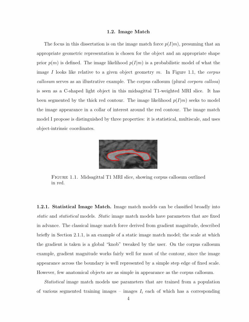
image I looks like relative to a given object geometry m. In Figure 1.1, the corpus

callosum serves as an illustrative example. The corpus callosum (plural corpora callosa)

is seen as a C-shaped light object in this midsagittal T1-weighted MRI slice. It has

been segmented by the thick red contour. The image likelihood p(I|m) seeks to model

the image appearance in a collar of interest around the red contour. The image match

model I propose is distinguished by three properties: it is statistical, multiscale, and uses

object-intrinsic coordinates.

Figure 1.1. Midsagittal T1 MRI slice, showing corpus callosum outlinedin red.

1.2.1. Statistical Image Match. Image match models can be classified broadly into

static and statistical models. Static image match models have parameters that are fixed

in advance. The classical image match force derived from gradient magnitude, described

briefly in Section 2.1.1, is an example of a static image match model; the scale at which

the gradient is taken is a global “knob” tweaked by the user. On the corpus callosum

example, gradient magnitude works fairly well for most of the contour, since the image

appearance across the boundary is well represented by a simple step edge of fixed scale.

However, few anatomical objects are as simple in appearance as the corpus callosum.

Statistical image match models use parameters that are trained from a population

of various segmented training images – images Ii each of which has a corresponding

4

segmentation mi that is taken as the “ground-truth” of the geometry of the object. Fig-

ure 1.2 illustrates a small population of corpora callosa, from various patients, suitable

for training a statistical model. The model-building process for a statistical image match

model samples each of the training images Ii relative to the given geometry mi to get an

idea of what the image “looks like” near the object. This implicitly assumes a definition

of correspondence, or homology, between objects in the training population. Generally

the correspondence is given by the shape representation of the objects, sometimes aug-

mented by manually-placed landmarks. Image-based features are derived from each of

the training images, and the features are used to train the statistical image match model.

A standard example of a statistical image match model is the one used by Active Shape

Models; it is described in more detail in Section 2.1.3.1. The image match model pro-

posed in this dissertation can be seen as an extension of the statistical image match

model used by Active Shape Models.

Figure 1.2. Population of corpora callosa, on which a statistical imagematch model could be trained.

1.2.2. Multiscale Image Match. Observations are taken with an aperture, and a sig-

nal may have components at various scales. The pixel size of an image, for instance an

MRI, represents observations taken at a particular scale that is set by the image acquisi-

tion process. However, the object of interest within the image might be best represented

5

at other scales. Others have worked on multiscale object geometry representations [Pizer

et al. 2003]; similarly, a multiscale representation of the image uses multiple apertures,

from coarse to fine, to sample the image. A multiscale image model can show at vari-

ous locations what are the scales at which the variability in the training population is

represented most tightly. For instance, in the corpus callosum example, the bulk of the

corpus callosum might be well-represented at a relatively large scale, since it is fairly

uniform white matter with a fairly consistent step-edge at the boundary. However, the

fornix (small white matter branch off the lower edge of the corpus callosum) is a relatively

small scale feature, so the image intensities at that location might be well-represented

at a relatively small scale. Classical single-scale image match models represent the im-

age only at the original pixel scale provided by the image acquisition process, rather

than finding natural local scales at which to represent the image, which may depend on

the object geometry, correspondence, signal-to-noise ratio, and population variability. A

number of image segmentation techniques have multi-grid extensions, which use multi-

scale techniques [Cootes et al. 1994, Willsky 2002]. The human visual system at some

level uses a multiscale approach [Romeny 2003].

Figure 1.3. Segmented corpus callosum. Arrow indicates the fornix, asmall scale white matter structure branching off from the lower boundaryof the corpus callosum. Consistent localization of the fornix across thepopulation motivates image match in object-intrinsic coordinates.

1.2.3. Image Match in Object-Intrinsic Coordinates. Object-intrinsic coordinates

are a local non-Euclidean coordinate system on the object, derived from the geometry

of the object, instead of the image acquisition process. The standard coordinate system

for images, for instance the Euclidean (x, y, z) coordinate system of 3D MRI, is provided

by the scanner in which the image was taken. If the orientation of a patient’s head

6

changes relative to the scanner, then the orientation of objects in the standard image

coordinate system changes as well. In the corpus callosum example, if it is desired to

localize the fornix consistently across the population of corpora callosa, then a system of

correspondence is needed that matches the fornix of one corpus callosum to the fornix

of another. An object-intrinsic coordinate system is a way of representing a continuum

of such correspondences in a region of interest around the object. The task of defining

correspondence, or homology, is a large issue [Davies 2002, Styner et al. 2003] that is

outside the scope of this work, but my image match method depends on having a cor-

respondence given. If a different system of correspondence is provided, then my method

can take advantage of it just as easily.

My implementation uses the spherical harmonics (SPHARM) shape representation

for the object boundary, which decomposes the (x, y, z) coordinates of boundary points

using spherical harmonic basis function. A system of correspondence based on an equal-

area parameterization is also provided by this shape representation. The SPHARM

shape representation will be described in Section 2.2 and in further detail by [Kelemen

et al. 1999]. Potential extensions to other shape representations will be described in

Section 5.4.5.

To sample the image using object-intrinsic coordinates instead of Euclidean image

coordinates, I use image profiles. Profiles are samples taken from the image along 1-

dimensional paths intersecting the object boundary. A collection of profiles about a

particular geometric object within a particular image is a representation of the region

within that image that is of interest for localizing the boundary. For example, profiles may

capture a step-edge in intensity at the boundary of the corpus callosum. The particular

profile sampling scheme I use will be discussed in more detail in Section 3.1.6.

1.3. Case Study: Caudate

Many segmentation methods use an image match that locally drives the object bound-

ary to points of high image gradient magnitude. The classical “snakes” [Kass et al. 1987a],

7

for instance, uses this approach. In many objects, however, a simple gradient-magnitude

based image match model is insufficient. The profile of the image across the object bound-

ary can vary significantly from one portion of the boundary to another. Some portions

of the boundary might not even have a visible contrast, in which case the shape prior

may be needed to define the contour. In real-world medical images, the contrast-to-noise

ratio is often low, and models need to be robust to image noise.

In this work, the target anatomical object for segmentation is the caudate nucleus in

the human brain. From a partnership with the UNC Psychiatry Department, access is

provided to over 100 high-resolution MRIs with high-quality manual expert segmenta-

tions of both left and right caudates. The manual raters, having spent much effort on

developing a reliable protocol for manual segmentation, indicate some of the challenges

in caudate segmentation, which motivate a multiscale statistical image match model for

automatic methods.

A fraction of the surface of the caudate borders the lateral ventricle, providing strong

contrast between the uniform grey matter of the caudate with the cerebro-spinal fluid

(CSF) of the ventricle. Other portions of the caudate border white matter tracts, pre-

senting a different image profile, which is still fairly consistent at corresponding locations

across the training population.

Portions of the boundary of the caudate can be localized with standard edge detection

(provided the appropriate scales are chosen). However, there are also nearby false edges

that may be misleading. In addition, where the caudate borders the nucleus accumbens,

there is no contrast at the boundary; the manual raters use a combination of shape

prior and external landmarks to define this part of the boundary. Figure 1.4 shows the

challenge. The caudate and nucleus accumbens are distinguishable on histological slides,

but not on MRI of this resolution.

Another “trouble-spot” for the caudate is where it borders the putamen; there are

“fingers” of cell bridges that span the gap between the two. The scale of the object struc-

ture relative to the scale of the image noise may swamp single-scale image match models

8

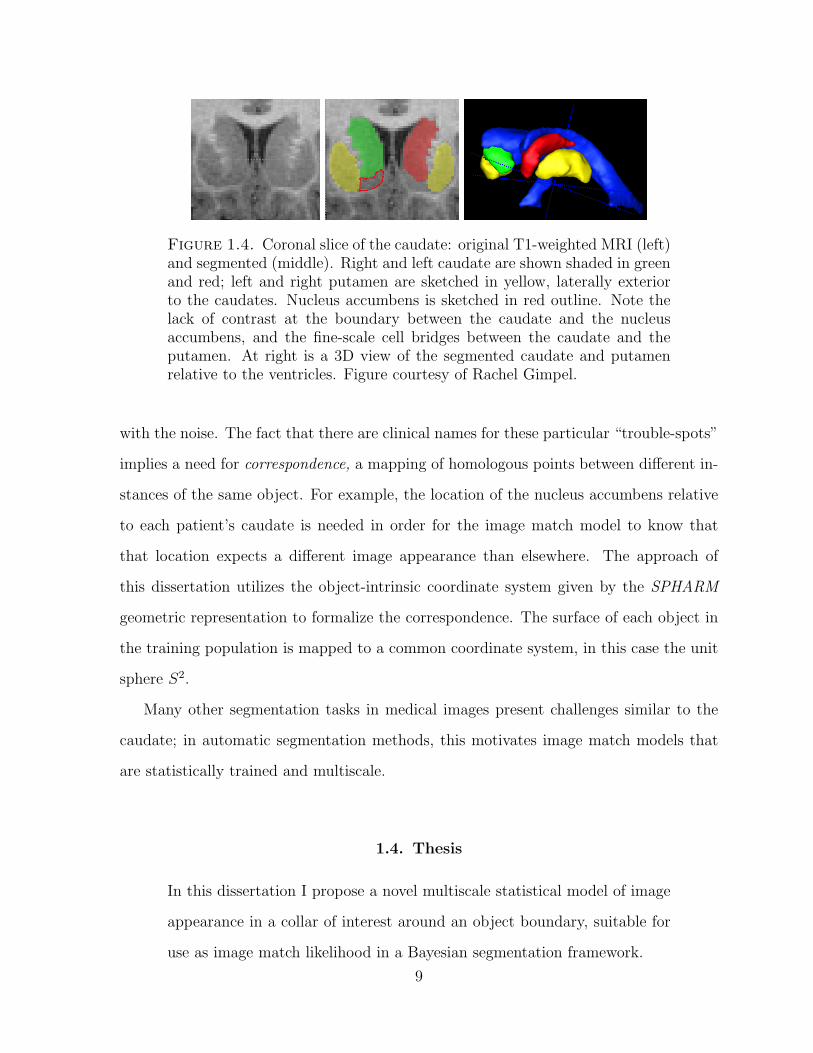
Figure 1.4. Coronal slice of the caudate: original T1-weighted MRI (left)and segmented (middle). Right and left caudate are shown shaded in greenand red; left and right putamen are sketched in yellow, laterally exteriorto the caudates. Nucleus accumbens is sketched in red outline. Note thelack of contrast at the boundary between the caudate and the nucleusaccumbens, and the fine-scale cell bridges between the caudate and theputamen. At right is a 3D view of the segmented caudate and putamenrelative to the ventricles. Figure courtesy of Rachel Gimpel.

with the noise. The fact that there are clinical names for these particular “trouble-spots”

implies a need for correspondence, a mapping of homologous points between different in-

stances of the same object. For example, the location of the nucleus accumbens relative

to each patient’s caudate is needed in order for the image match model to know that

that location expects a different image appearance than elsewhere. The approach of

this dissertation utilizes the object-intrinsic coordinate system given by the SPHARM

geometric representation to formalize the correspondence. The surface of each object in

the training population is mapped to a common coordinate system, in this case the unit

sphere S2.

Many other segmentation tasks in medical images present challenges similar to the

caudate; in automatic segmentation methods, this motivates image match models that

are statistically trained and multiscale.

1.4. Thesis

In this dissertation I propose a novel multiscale statistical model of image

appearance in a collar of interest around an object boundary, suitable for

use as image match likelihood in a Bayesian segmentation framework.

9

This model significantly improves specificity and variance over a classi-

cal single-scale profile model, as demonstrated on a large-scale MRI study

of the caudate nucleus, evaluating generalizability, specificity, and variance.

Validation also compares automatic segmentation using my image match

model, automatic segmentation using a classical single-scale model, and

expert manual segmentation.

1.5. Accomplishments

Much of the work in this dissertation builds upon existing work of others in the field.

The novel contributions that I present include

• A scale space for functions on manifolds that are diffeomorphic to the sphere S2,

• A scale space for boundary profiles of simply-connected objects, which is a new

scale space in object-intrinsic coordinates,

• A probabilistic model for boundary profiles, using the above scale space,

• A complete, self-contained software framework for model-building and segmen-

tation, using the above probabilistic model for image match,

• Validation of the results from the above segmentation framework, on a sizeable

population of 114 caudate datasets, with manual rater segmentations,

• Evaluation of the generalizability, specificity, and statistical efficiency of the

above probabilistic model for boundary profiles.

1.6. Overview of the Chapters

This dissertation is organized in five chapters. This chapter introduced the task

at hand, namely the construction of a multiscale statistical image match model, and

provided some motivation why such an image match model is useful. Chapter 2 will

provide background material to the dissertation, discussing other image match models in

use in popular Bayesian model-based segmentation schemes. Particular attention will be

given to the SPHARM segmentation framework, upon which the shape prior of my work

is based. The background chapter also will discuss various axiomatic approaches to scale

10

space. Chapter 3 will describe my multiscale statistical image match model. The first

section in the chapter will define a scale space on image profiles taken about the boundary

of the object in the image. The second section will describe features sampled from that

profile scale space, which are then used in a Markov random field probabilistic model.

Chapter 4 will describe the testbed implementation in Mathematica, the datasets used,

and validation of the claims of the thesis. The image match model will be evaluated on

its own as a probabilistic model; it will also be evaluated as a component of a complete

segmentation framework in conjunction with a shape prior. Comparisons will be made

of the new multiscale image match model against the classical single-scale image match

model. Chapter 5 will conclude with proposed future work, possible extensions and new

applications.

11

CHAPTER 2

Background

2.1. Image Match Models in Deformable-Models Segmentation

Deformable models have had a long history in image segmentation, and each method

uses some form of image match to drive the deformable model into the target image.

Image match is sometimes also referred to as “image energy” or “external forces”, in

contrast to the shape prior, or “internal forces”. Even with non-Bayesian segmentation

models, there is always a driving force that instantiates the model into a particular

target image. The focus of this dissertation is a new multiscale statistical image match

model; in this chapter I present a selection of existing image match models in use in

deformable-models image segmentation.

2.1.1. Gradient Magnitude “Edge Finding”. Perhaps the simplest image match

model is simply to use the magnitude of the gradient vector of the image intensity field.

In the classical snakes [Kass et al. 1987b], the image match force pushes each contour

point towards a local maximum of image gradient magnitude. The degree of match of

the whole contour into the image is the integral along the contour C of the local image

gradient magnitude |∇I|:

p(I|m) ∝∫

C

|∇I(x)|dx.

This integral does not yield a probability distribution on its own, but the Bayesian

image match probability distribution is usually some monotonic function of the integral

of gradient magnitude.

The gradient magnitude is one example of a translation and rotation invariant feature

that can be used to drive the image force. Other examples include the Harris corner

detector [Harris and Stephens 1988] and affine-invariant corner detectors [Blom 1991].

Gradient magnitude is often used by both mesh-based snakes and implicit (geodesic)

snakes [Malladi et al. 1995, Caselles et al. 1997]. This works well for clearly defined objects

whose boundary is always characterized by a sharp discontinuity in image intensity.

However, this image match model is global (it assumes the boundary appearance is

uniform across the whole object) and static (it is not statistically trained). The gradient

magnitude is often calculated at a fixed scale at all points along the contour; hence it

assumes that the desired edges in the image are all at the same scale. Gradient magnitude

image match performs poorly at weak or nonexistent step edges, or when the boundary

discontinuity is not well-represented by a step edge.

2.1.2. Static Template Matching.

2.1.2.1. Inside/Outside Classification. Region-competition snakes use global probability

distributions of “inside” intensities vs. “outside” intensities to drive the image match [Zhu

and Yuille 1995, Tek and Kimia 1997]. van Ginneken et al. perform a local inside/outside

classification using not just the raw greylevels but a high-dimensional n-jet feature vector,

with k nearest-neighbor (k-NN) clustering and feature selection, based on the training

population [van Ginneken et al. 2001]. Leventon et al. train a global profile model

that relates intensity values to signed distances from the boundary, incorporating more

information than a simple inside/outside classifier [Leventon et al. 2000].

2.1.2.2. Profile Templates. Segmentation via registration to a template image or atlas is

a common technique.

For example, the medially-based m-reps deformable model segmentation framework [Joshi

et al. 2001] can use image intensities taken from a single template image to drive its im-

age match forces. The normalized correlation between corresponding intensities in the

template image and in the target image provides the image match. This takes advan-

tage of the correspondence given by the medially-defined figural coordinate system in a

13

volumetric collar about the object boundary, implied from the geometric representation.

Normalized correlation is equivalent to a local Gaussian model on each profile, where the

mean is the template profile and the covariance matrix is diagonal. It assumes that in-

tensities at different positions along the profile are uncorrelated. The profile model which

I will present explicitly models the correlation between intensities at different positions

along a profile, as well as the correlation between adjacent profiles along the boundary.

Profiles have also been used in 2D cardiac MR images [Duta et al. 1999]. Fenster et

al. have extracted features from profiles for use in fitting their Sectored Snakes [Fenster

and Kender 2001].

2.1.2.3. Image Warping. In the fluid warping techniques of Joshi et al. [Miller et al. 1999],

a template image is warped to the target image via a diffeomorphic map. Manually-placed

landmarks in both template and target images guide the optimization of the diffeomorphic

map, but the match between template and target images is measured by the integrated

squared-difference between image intensities in MRI:

(4) D(h) =

∫Ω

|T (h(x))− S(x)|2dx,

where T (h(x)) is a sample from the warped template image, S(x) is a sample from the

target image, and Ω is the region of interest. The image energy term in the optimization

is a combination of D(h) and a term that optimizes the manually-placed landmarks.

Image match by profile templates can be seen as a special case of image match by

fluid warping, where the region of interest is the collar about the boundary where the

profiles are taken. Joshi et al. also take special care to ensure the warp from target image

to template image is diffeomorphic.

2.1.2.4. Mutual Information. The sum of squared-differences in image intensity is not the

only metric of image match that can be used to match the template to the target image.

For example, recent work of Tsai et al. uses mutual-information between regions of the

image and a label map to drive the segmentation [Tsai et al. 2003, 2004]. Willis [2001]

also use mutual information between a template image and the warped target image.

14

2.1.3. Probabilistic Models.

2.1.3.1. Statistical Profile Model. Cootes and Taylor’s seminal Active Shape Model work [Cootes

et al. 1993] samples images along 1D profiles around boundary points, normal to the

boundary, using correspondence given by the Point Distribution Model of geometry. At

each point along the boundary, a probability distribution is trained on the image-derived

features in the 1D profile (ASMs use the derivative of image intensity along the profile).

The corresponding profile is sampled from the target image, and the Mahalanobis dis-

tance in the probability distribution at that boundary point provides the image match.

Recently Scott et al. expanded the feature space used in the profiles [Scott et al. 2003].

The ASM profile model has been used with 2D Fourier [Staib and Duncan 1992]

coefficients as the shape representation instead of PDMs.

A statistical model built from a few select profiles was also described by Duta et al.

and applied to cardiac MR images [Duta et al. 1999].

The “hedgehog” model in the spherical harmonic segmentation framework [Kelemen

et al. 1999] uses a training population linked with correspondence from the geometric

model. It can be extended with a coarse-to-fine sampling of the object boundary in order

to improve robustness in the face of image noise and jitter in correspondence.

Recent work by Stough et al. on profiles for m-reps uses clustering to elect a small

number of representative profile types, then classifies boundary patches according to

profile type [Stough et al. 2004].

Van Ginneken [van Ginneken et al. 2001] discriminates between profiles at correct

boundary positions and profiles shifted normal to the boundary, for use in localizing the

object boundary.

2.1.3.2. Active Appearance Models. A different approach is taken by Cootes and Taylor’s

Active Appearance Models [Cootes et al. 2001], which use the point correspondences

given by an ASM to warp images into a common coordinate system, within a region of

interest across the whole object, given by a triangulation of the PDM. A global Principal

Components Analysis is performed on the intensities across the whole object (the size

15

of the feature space is the number of pixels in the region of interest). To improve the

optimization process, global PCA are performed on the registered images blurred at

various scales. The use of a global PCA is particularly well-suited for capturing global

illumination changes, for instance in Cootes and Taylor’s face recognition applications.

2.1.4. Summary and Limitations of Existing Work. Real world images and also

medical imagery, for example, exhibit complex discontinuities at the object boundary.

Moreover, discontinuities can have different characteristics at different locations along

the boundary. For instance, object could be expected to have a step edge at one part

of the boundary but a line-like edge at another part along the boundary. It is clear

that gradient magnitude, especially at fixed global scale, is not sufficient to capture

complex image characteristics. A robust image match model also needs to be trained

from a population of images; a single template is not sufficient. Current profile models

capture local variation, but they do not take advantage of the expected high degree of

correlation between adjacent profiles along the boundary. Normalization of the profiles

is also an issue; selection of appropriate image-derived features is important. Active

Appearance Models are very promising and closely related; this work can be interpreted

as an extension of ASMs to capture local intensity variation in a hierarchical fashion.

It is desired that an image match model be robust enough to capture local intensity-

derived features about the boundary, while being aware of the distinction between the

along-boundary and across-boundary directions, already defined by the geometric model.

Across the boundary, one would like to know if the image locally should be expected to

present a step edge, or a line-like edge, or something else, at different scales. Along the

boundary, one would like to take advantage of spatial locality in order to provide robust-

ness to image noise and jitter in the provided correspondence. The image characteristics

about a single point on the boundary may be noisy and difficult to model, but perhaps

by averaging over a larger portion of the boundary, it may be evident that a line-like

edge for instance is expected at this patch of the object boundary.

16

It is also important that a framework exists for examining the training images sampled

at corresponding points so that statistical models can be built of the intensity variation

about the boundary. There are many potential sources of image noise in the image

acquisition process. For instance, in MRIs, challenges include MR noise, scanner stability,

and bias field inhomogeneity, in addition to patient induced variations of brightness and

contrast as well as inter-object variability (e.g., motion of adjacent structures). An image

match model is desired that can capture image characteristics about the object boundary

despite noise, in order to improve segmentation.

Image features at the boundary may appear at various scales, which motivates a

multiscale approach. However, traditional multiscale features blur in Euclidean space,

which may blur across the object boundary. In the spirit of Canny [Canny 1986], mul-

tiscale features are desired where the blurring is along the boundary and not across the

boundary.

My approach is to construct a scale space on the image profiles, similar to classical

scale-spaces [Koenderink 1984, Florack et al. 1996] but on a curved non-Euclidean space.

I then sample the profile scale space after the fashion of Laplacian image pyramids [Burt

and Adelson 1983] to obtain multiscale features upon which Gaussian models are trained

using the training population. The end result is a likelihood model for geometry-to-image

match; this combined with the shape prior produces the posterior that is to be optimized

in Bayesian segmentation.

17

2.2. The SPHARM Segmentation Framework

Any image match model for Bayesian segmentation will be closely tied to the geo-

metric representation used for the object to be segmented – whether a boundary rep-

resentation, medial representation, volumetric representation, or other representation of

the object. The general concept presented in this dissertation is applicable to various

geometric representations, but the details are necessarily tied to a particular geomet-

ric representation. I choose to use the SPHARM shape representation of Brechbuhler et

al. [C. Brechbuhler and Kubler 1995]. Kelemen et al [Kelemen et al. 1999] used this shape

representation in conjunction with an ASM-style single-scale statistical profile model to

produce a full Bayesian segmentation framework. This section is a brief review of that

work; for more details refer to the above citations and the dissertations of Brechuhler

and Kelemen.

The SPHARM shape representation uses an orthogonal basis expansion of the (x, y, z)

coordinates of points on the object boundary. The spherical harmonics Y ml are a com-

plete orthonormal basis for L2(S2), functions on the unit sphere S2. The exact definition

will be given in Section 3.1.2. A mesh of equally-spaced points (xi, yi, zi) on the surface

of the simply-connected object is parameterized by three functions (x(θ, φ), y(θ, φ), z(θ, φ))

on S2; each is expanded in the spherical harmonic basis:

x(θ, φ) =∑l,m

cxml Y m

l (θ, φ)(5)

y(θ, φ) =∑l,m

cyml Y m

l (θ, φ)(6)

z(θ, φ) =∑l,m

czml Y m

l (θ, φ).(7)

The set of spherical harmonic coefficents cml = (cx

ml , cy

ml , cz

ml ) forms the geometric

representation of the object. The abbreviation SPHARM is used to refer to these cml

as a shape representation, or to refer to Kelemen’s complete segmentation framework

using this shape representation (“the SPHARM segmentation framework”).

18

The parameterization of the surface of the object, in the form of the three functions

(x(θ, φ), y(θ, φ), z(θ, φ), is itself a complex optimization problem. The parameterization

is constrained to preserve areas: patches of equal area on the original object map to

patches of equal area on the parameter space (S2). Angles cannot be preserved exactly,

but squares on the original object are optimized to map to approximate squares on

S2. This parameterization defines a point-to-point correspondence between instances of

an object: for example, it defines a north pole on each of the instances of an object.

My implementation uses the equal-area parameterization given by SPHARMs, but the

method can take advantage of other definitions of correspondence when provided.

A reasonable shape prior for a Bayesian segmentation framework using the SPHARM

shape representation is a Gaussian distribution on the spherical harmonic coefficients

cml of normalized objects. The surface of each object in the training population is

parameterized and expanded in the spherical harmonic basis. The coefficients are then

normalized to factor out global translation and rotation, and a multidimensional Gaussian

model is built on the resulting normalized coefficients:

p(m) = p(cml )(8)

= N(µc, Σc)(c),(9)

where N(µc, Σc)(c) represents the Gaussian likelihood of the coefficient set c in the

multidimensional normal distribution with mean shape µc and covariance matrix Σc. In

usual implementation, the spherical harmonics are expanded to order 12, resulting in a

feature space of dimension 504. This is the shape prior used in this dissertation work.

Kelemen’s SPHARM segmentation framework is inspired by ASMs and does not in

fact use the above Gaussian shape prior model; rather, it uses a constrained optimization

approach where the segmentation is allowed to deform freely within a box of “allowable”

shapes (e.g., within ±2 standard deviations in the first five eigenmodes of deformation).

This is equivalent to a shape prior that is uniform within the box of allowable shapes

and zero outside the box.

19

The image match model in Kelemen’s SPHARM segmentation framework uses image

profiles at the object boundary. The SPHARM shape representation provides a param-

eterized surface for the boundary of the object, which in particular allows normals to

the boundary to be computed analytically. For each object in the training population,

its corresponding image is sampled along a number of straight lines perpendicular to the

boundary and crossing it. Section 3.1.6 will discuss the issue of how profiles are sampled:

I use the same sampling method as the SPHARM framework does, but it does have a

number of problems. Figure 2.1 illustrates the locations from which profile samples are

taken; they appear like quills on a hedgehog. Thus for each object n in the training

population, at each corresponding location i on the boundary, there is a vector uni of

image intensities sampled across the boundary. In sample implementations there may be

114 training objects, 512 profiles around the object boundary, and 11 samples along each

profile.

Figure 2.1. Visualization of the profiles extracted from the boundary ofthe caudate. Profiles are shown as white “quills” normal to the boundary.

In the single-scale profile model used by Kelemen and inspired by ASMs, each position

along the boundary has an independent Gaussian profile model: each ui is modeled by

its own normal distribution N(µi, Σi). With the above numbers, there would be 512

independent 11-dimensional Gaussians. The overall Bayesian likelihood is simply the

20

average of the likelihoods at each profile:

p(I|m) = p(ui)(10)

=1

N

∑i

p(ui)(11)

=1

N

∑i

N(µi, Σi)(ui),(12)

where N is the number of profiles around the boundary (e.g., 512). N(µi, Σi)(ui) rep-

resents the Gaussian likelihood of ui in the multidimensional normal distribution with

mean µi and covariance matrix Σi.

During segmentation, at each iteration of deformation the spherical harmonic coeffi-

cients c are calculated from the deformed shape and compared against the shape prior

model. Profiles u are also taken from the deformed segmentation and compared against

the image match models. Each profile ui is fit against the local profile model at various

shifts normal to the boundary; the optimal shift is a suggested local deformation of the

boundary. The suggested deformations dx are transformed into perturbations db in the

shape eigenspace and constrained to lie within the “box” of allowable deformations.

In this dissertation I use the SPHARM shape representation and segmentation frame-

work as a platform to explore multiscale extensions to the profile model with a non-

Euclidean scale space that follows the object boundary. The testbed implementation

uses a Gaussian shape prior as described above. It allows comparison of the conventional

single-scale profile model to my new multiscale profile model. The implementation will

be described in more detail in Section 4.1.

21

2.3. Approaches to Scale Space

Since my new image match model is a multiscale extension to the standard profile

model used in ASMs and Kelemen’s SPHARMs, I review a selection of prior work on the

issue of scale from the perspective of scale space. Observations are always taken at scale;

the original resolution of the image is only a result of the image acquisition process. The

natural scale at which objects or signals exist may be different from the image acquisition

resolution. In addition, fine-scale image noise often clouds the signal, and this motivates

multiscale approaches that can model the signal at its appropriate scale while separating

out the image noise.

A scale space is an image defined on the product space of the domain of the original

image with the scale axis R+; it is a way of representing an image at all scales simulta-

neously. If the original image is a scalar function in d-dimensions, f : Rd → R, a scale

space of f would be a function Φ(f) : Rd×R+ → R. I define an observation at scale as a

particular point in scale space; how scale space is constructed defines what is meant by

“scale”. For a given scale σ, a cross-section Φ(f)(x, σ) : x ∈ Rd through the scale space

represents the image blurred at scale σ. Figure 2.2 shows an illustration of a scale-stack

in R2 × R+, a number of slices through the scale space at various scales σ.

Figure 2.2. Illustration of a scale-stack, a sampling of continuous scalespace that is discrete in scale. Shown are scales σ = 0.5, 1.5, 2.5, 3.5, and4.5.

22

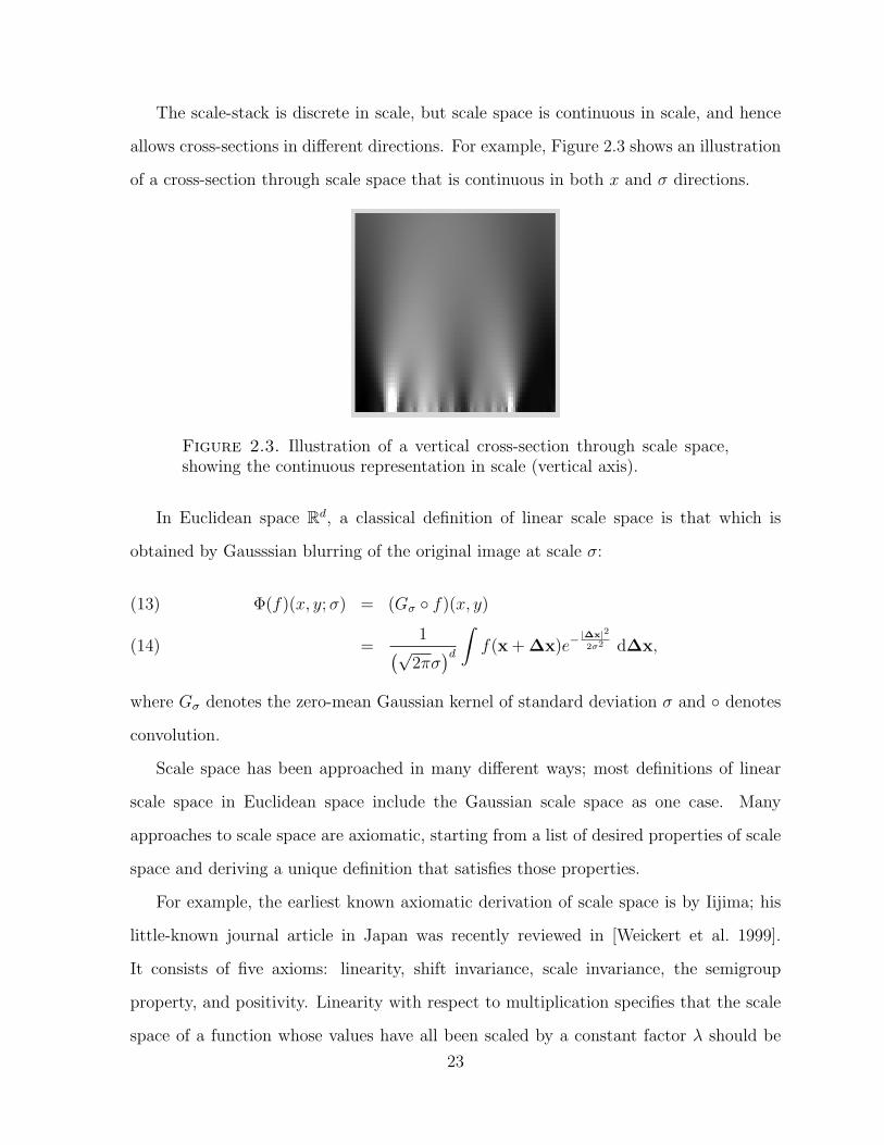
The scale-stack is discrete in scale, but scale space is continuous in scale, and hence

allows cross-sections in different directions. For example, Figure 2.3 shows an illustration

of a cross-section through scale space that is continuous in both x and σ directions.

Figure 2.3. Illustration of a vertical cross-section through scale space,showing the continuous representation in scale (vertical axis).

In Euclidean space Rd, a classical definition of linear scale space is that which is

obtained by Gausssian blurring of the original image at scale σ:

Φ(f)(x, y; σ) = (Gσ f)(x, y)(13)

=1(√

2πσ)d ∫ f(x + ∆x)e−

|∆x|2

2σ2 d∆x,(14)

where Gσ denotes the zero-mean Gaussian kernel of standard deviation σ and denotes

convolution.

Scale space has been approached in many different ways; most definitions of linear

scale space in Euclidean space include the Gaussian scale space as one case. Many

approaches to scale space are axiomatic, starting from a list of desired properties of scale

space and deriving a unique definition that satisfies those properties.

For example, the earliest known axiomatic derivation of scale space is by Iijima; his

little-known journal article in Japan was recently reviewed in [Weickert et al. 1999].

It consists of five axioms: linearity, shift invariance, scale invariance, the semigroup

property, and positivity. Linearity with respect to multiplication specifies that the scale

space of a function whose values have all been scaled by a constant factor λ should be

23

obtainable by multiplying the values of the original scale space by the same factor:

(15) Φ(λf) = λΦ(f).

Shift invariance specifies that the scale space of a translated function should just be the

translated scale space of the original function:

(16) Φ(Ts0(f)) = Ts0(Φ(f)),

where Ts0 represents a translation operator acting on functions, shifting by an amount

s0. In Rd, Tx0(f)(x) = f(x−x0). Scale invariance requires that the scale-space operator

should be invariant to the scale of a function:

(17) Φ(Sc(f)) = Sc(Φ(f)),

where Sc represents a scaling operator acting on functions, enlarging the scale of the

function by a factor c. In Rd, Sc(f)(x) = f(x/c). The semigroup property means that

blurring via the scale space should “cascade”:

(18) Φ(fσ1)(s, σ2) = Φ(f)(s, σ1 + σ2),

where fσ1(s) = Φ(f)(s, σ1) as above. The axiom of positivity specifies that the scale

space of an everywhere-positive function should be everywhere-positive:

(19) f(s) > 0 ∀s =⇒ Φ(f)(s, σ) > 0 ∀s, σ.

As a boundary condition ensuring that the scale space represents the original signal at

zero scale, one more axiom is added requiring that the scale space of a function f converge

uniformly to f as the scale σ goes to 0.

Iijima’s axiomatic is only one set of axioms for scale space, though, and there are

others. Florack uses another set of axioms, starting from linearity, shift invariance,

and scale invariance, and adding isotropy (rotation invariance) [Florack et al. 1992].

24

ter Haar Romeny has used similar axiomatics derived from the human front-end vision

system [Romeny 2003].

Koenderink introduced the axiom of causality, that no new information should be

created as one goes up in scale (to coarser scale). His early foundational work used this

axiom together with linearity and isotropy to derive the Gaussian scale space [Koenderink

1984]. A concise overview diagram of a number of scale space axiomatics is in [Kuijper

2003].

An observation made by Koenderink, ter Haar Romeny, Lindeberg [Lindeberg 1994],

and others is that a number of standard axioms for scale space lead to a particular partial

differential equation which the scale space needs to satisfy, namely, the heat equation:

(20)∂u

∂t= 4u.

Boundary conditions on the solution specify that as the scale parameter t goes to zero,

u approaches the original image f . The linear operator 4 can also be expressed as

div(∇u). The heat equation approach to scale space will be discussed in more detail in

Section 3.1.1. This is the approach to scale space that I adopt: in Chapter 3 a scale

space will be proposed as a solution to the heat equation in a non-Euclidean space.

Duits has modified the heat equation by adding a fractional power α ∈ (0, 1] to the

linear operator 4:

(21)∂u

∂t= −(−4)αu.

This results in a family of scale-spaces, of which the Gaussian scale space is a special case

at α = 1. The case α = 1/2 leads to a scale space generated by the Poisson operator.

The α scale spaces satisfy all the classical axioms of scale space, using a weak version of

the causality axiom [Duits et al. 2004].

Various non-linear scale-spaces have also been described on the Euclidean domain;

they violate the axiom of linearity but can be useful for edge-enhancement. For example,

Perona and Malik proposed a non-linear diffusion process that modifies the classical heat

25

equation to become

(22) u(x, t) = div · (g(|∇f |)∇f) ,

where g is a monotonically decreasing function [Perona and Malik 1990]. The idea is to

reduce the blurring around “edges” (as detected by g(|∇f |)) so as to preserve the edge

structure. Anisotropic diffusion blurs in different amounts along different directions; the

aim is to blur parallel to an edge but not across the edge [ter Haar Romeny 1994].

These non-linear and anisotropic scale spaces use local image information (such as

the image gradient) to determine where to blur and in what directions to blur. The scale

space I will define is inspired by the same concept of blurring along the boundary but

not across it. However, rather than the image gradient, my method uses the boundary

given by the segmentation geometry. The blurring is performed using not the Euclidean

metric, but a metric implied by the geometric representation of the object: an object-

intrinsic coordinate system. The profile scale space I will define in the next chapter takes

advantage of a definition of correspondence given by the geometric representation.

26

CHAPTER 3

Methods

My objective in this dissertation is to define a measure of geometry-to-image match,

i.e., a measure of how well a given geometric object fits into a target image. Such a

measure is specified as a probability distribution on image intensity features in a region

of interest about the object boundary. In this chapter, the image features are defined

and a probability distribution is then imposed on those features. An important construct

defined here is the profile scale space, which allows analysis of image profiles of the

boundary at various scales, while not blurring away contrast across the boundary. The

profile scale space is sampled according to a hierarchical tree structure, and the resulting

multiscale image features, across the training population, are modeled with a Markov

Random Field probability distribution. Throughout this chapter, the notation is specific

to objects in 3D images, but most of the theory can be extended naturally to arbitrary

dimension.

I start in Section 3.1.1 by discussing my approach to scale space from the perspective

of the heat equation and the Laplacian operator. This approach allows me to define

in Section 3.1.2 a scale space for scalar-valued functions defined on the sphere S2. The

sphere is simpler geometrically than the boundary of a generic object, but it still presents

some interesting challenges in comparison to Euclidean space.

Section 3.1.3 makes use of the scale space on S2 to define a scale space for scalar

functions on arbitrary object boundaries that are diffeomorphic to S2, via a diffeomorphic

mapping provided by a spherical harmonic representation of the object. This scale space

is not the same as that obtained by Laplace-Beltrami smoothing; Section 3.1.4 briefly

compares the two.

In Section 3.1.5, I review a few properties that have been used as axioms to classical

derivations of scale space on Euclidean space. I then discuss those scale-space properties

that apply to these non-Euclidean domains, and I discuss whether my definition of scale

space satisfies these properties.

Section 3.1.6 then extends the scale-space concept from scalar-valued functions to

profiles across the object boundary, viewed as a product space of the boundary manifold

with the interval [−1, 1].

With the profile scale space defined, Section 3.2.1 describes a multiscale collection of

features sampled from the profile scale space. In the model-building phase these features

are extracted from each of the segmented training images and used to train a Markov

Random Field probabilistic model, as is described in Section 3.2.2. During segmentation

the same image features are extracted from the target image relative to the deformable

shape model in its current state of deformation. The probabilistic model defines the

match of the deformed shape model to the image.

3.1. The Profile Scale Space

3.1.1. Scale Space and the Heat Equation. To use multiscale features in modeling

the image, I first must define what is meant by scale. For instance, the boundary of

a particular object might be well-represented by a step-edge at a large patch of the

boundary; however, when the image is sampled at too fine of a scale, the image noise

overwhelms the edge structure. The aim is that a multiscale representation of such a

boundary patch could capture efficiently the step-edge profile at a large scale along the

boundary, while separating out the fine-scale noise.

As discussed in Section 2.3, classical scale-space theory in Euclidean space has often

used the analogy of heat distribution on a conducting plate [Lindeberg 1994]. The original

signal represents an initial distribution of heat on the plate; certain other boundary

conditions are also imposed. The temperature distribution on the plate equalizes over

28

time, according to the well-known differential equation describing heat flow:

(23)∂u

∂t= 4u,

where u(·, t) is the temperature distribution on the plate at time t. As t increases,

u(·, t) represents the signal at increasingly coarse scale (more blurring). If the initial

temperature distribution is a scalar-valued function f on R2, the scale space of f is a

scalar-valued function u on the product space R2 × R+.

The operator 4 is the Laplacian; in R2(x = (x, y)) the standard Laplacian is simply

(24) 4 =∂2

∂x2+

∂2

∂y2.

This operator on functions f ∈ L2(R2) also extends to an operator on scale-spaces u ∈

L2(R2 × R+):

(25) (4u)(x, y, t) = (4ut)(x, y),

where ut is a restriction of u to a plane in t, given by ut(x, y) = u(x, y, t).

The solution to the heat equation, with initial temperature distribution f(x) ∈

L2(R2), is

(26) u(x, t) = f(x)1√2πt

e−|x|2

t2 .

This solution is the classical linear scale space, or Gaussian blurring (see Equation 13).

The standard deviation of the Gaussian kernel used for blurring can be related to the

time parameter by the variable substitution t = 2σ2.

When the domain of the signal f is a bounded region of R2, the solution of the

heat equation depends on conditions placed at the boundary of the domain. There are a

variety of reasonable choices of boundary condition: for example, filling the plane outside

the region with zero, or filling the plane by extending the image periodically, or using

Neumann boundary conditions, which state that no image energy should enter or leave

the region.

29

A similar approach to scale space can be made when the domain of the signal f is

generalized from R2 to a general Riemannian manifold M with metric tensor g. The

Laplacian operator generalizes to an operator on L2(M), and the heat equation is the

same. The signal f ∈ L2(M) is the initial temperature distribution on the manifold

M. If the manifold has a boundary, then boundary conditions need to be imposed to

guarantee a unique solution to the heat equation. The solution to the heat equation

is a function u ∈ L2(M× R+) which represents the temperature at each point on the

manifold at each point in time.

A manifold embedded in Euclidean space inherits a metric tensor from the embed-

ding space; this is the Riemannian metric tensor. The Laplacian with the Riemannian

metric tensor is the Laplace-Beltrami operator; it is “coordinate-free” in that it does not

depend on any parameterization of the manifold but only on the local geometry of the

manifold. Chung et al. have used discrete approximations to the Laplace-Beltrami op-

erator for smoothing on the cortical surface of the brain [Chung et al. 2001]. Desbrun et

al. show a discrete implementation of the Laplace-Beltrami operator on general triangle

meshes [Desbrun et al. 1999]. The Laplacian can also be formed with an arbitrary metric

tensor on the manifold M, not just the Riemannian metric tensor. The approach I use

to develop a scale space on the manifold M uses a diffeomorphic map from the sphere S2

to M. The map together with the natural metric tensor on S2 implies a metric tensor

on M; the scale space I develop in Section 3.1.3 is a solution to the heat equation on M

using that metric tensor. The connection between my scale space and Laplace-Beltrami

smoothing is explored in Section 3.1.4.

3.1.2. Scale Space on the Sphere S2. In this section I extend the heat-equation scale-

space theory from scalar functions on Euclidean space to scalar functions on S2. The

theory in this section is from joint work with Remco Duits of the Technical University

of Eindhoven in the Netherlands.

Let f : S2 → R be a function defined on S2, the unit 2-sphere, which can be thought

of as the surface of the unit ball in R3. S2 can be parameterized by colatitude θ ∈ [0, π]

30

and azimuth φ ∈ [0, 2π]. With this parameterization there are coordinate singularities

along the prime meridian (φ = 0, 2π), including the north and south poles (θ = 0 and

θ = π). For f to be well-defined in this parameterization, assume that f(θ, 0) = f(θ, 2π)

for all θ. Also assume that f(0, φ1) = f(0, φ2) and f(π, φ1) = f(π, φ2) for all φ1, φ2. The

surface area element ds on S2 is sin θ dθ dφ. Let f ∈ L2(S2), i.e.,

||f ||2 =

∫S2

|f |2ds =

∫ 2π

φ=0

∫ π

θ=0

|f(θ, φ)|2 sin θ dθ dφ < ∞

The Laplace operator on S2 is

(27) 4S2 =∂2

∂θ2+

cos θ

sin θ

∂

∂θ+

1

sin2 θ

∂2

∂φ2.

To solve the heat equation ∂u/∂t = 4u on S2, I use a spectral solution, which

uses eigenfunctions of the Laplacian linear operator. On S2, the eigenfunctions of the

Laplacian are a family of functions Y ml known as the spherical harmonics: they satisfy

(28) 4S2Y ml + l(l + 1)Y m

l = 0,

where the eigenvalue corresponding to each Y ml is l(l + 1). For a proof that the spherical

harmonics are eigenfunctions of the Laplace operator on S2, see [Muller 1966].

Definition 1. The spherical harmonics on S2 are functions Y ml : S2 → C given by

(29) Y ml (θ, φ) =

√2l + 1

4π

√(l −m)!

(l + m)!Pm

l (cos θ)eimφ,

where Pml (x) is the associated Legendre polynomial.

The degree l of the spherical harmonic ranges from 0 to ∞. The order m within each

degree l ranges from −l to l.

The spherical harmonics Y ml also form a complete orthonormal basis for L2(S2) [Muller

1966], hence any f ∈ L2(S2) has a Fourier expansion in spherical harmonics:

(30) f(θ, φ) =∞∑l=0

l∑m=−l

cml Y m

l (θ, φ),

31

where cml are the complex coefficients of the spherical harmonics:

(31) cml =

∫ 2π

φ=0

∫ π

θ=0

f(θ, φ)Y ml (θ, φ) sin θ dθ dφ

The scale space on S2 I propose is the spectral solution of the heat equation, using

the spherical harmonics as eigenfunctions of the Laplacian.

Proposition 1. Let f ∈ L2(S2), and let cml be its spherical harmonic coefficients,

as described above. The scale space of f I propose is Φ(f) : S2 × R+ → R given by

(32) Φ(f)(θ, φ; t) =∞∑l=0

l∑m=−l

e−l(l+1)tcml Y m

l (θ, φ).

The scale parameter σ can also be used, with t = 2σ2.

It is straightforward to check that this scale space satisfies the heat equation on S2:

∂

∂tΦ(f) =

∂

∂t

∞∑l=0

l∑m=−l

e−l(l+1)tcml Y m

l (θ, φ)(33)

=∞∑l=0

l∑m=−1

(∂

∂te−l(l+1)t

)cml Y m

l (θ, φ)(34)

=∞∑l=0

l∑m=−1

(−l(l + 1)e−l(l+1)t

)cml Y m

l (θ, φ)(35)

=∞∑l=0

l∑m=−1

e−l(l+1)tcml (−l(l + 1)Y m

l (θ, φ))(36)

=∞∑l=0

l∑m=−1

e−l(l+1)tcml (4Y m

l (θ, φ))(37)

= 4Φ(f).(38)

3.1.3. Scale Space on the Boundary Manifold M. Let the manifold M be the

boundary of the object to be segmented. For 3D objects, M is a 2-dimensional manifold.

Assume that M is differentiable and can be mapped diffeomorphically to the sphere

S2. Boundaries of simply connected objects generically will fit these assumptions. Let

32

f ∈ L2(M) be a scalar function on the manifold. For instance, f might be the image

intensity at the boundary of the object.

To define this scale space on M, I make use of the scale space on the unit sphere S2

discussed in Section 3.1.2. Let h : S2 → M denote a diffeomorphism between the unit

sphere and the object boundary. The SPHARM geometric representation provides one

such diffeomorphism, since the parameter space of the spherical harmonics is the unit

sphere. Since it is a diffeomorphism, it also has an inverse h−1 : M → S2. I use the

mapping h to define a pull-back of f onto S2, call it f ∗ : S2 → R, defined by f ∗ = f h:

(39) f ∗(θ, φ) = f(h(θ, φ)).

Since f ∗ is a function on S2, I can apply the scale space proposed in Section 3.1.2 to it.

The scale space on M I propose is Φ(f) : M× R+ given by

(40) Φ(f)(s, σ) = Φ(f ∗)(h−1(s), σ),

where s ∈M and Φ(f ∗) is the scale space on S2 given in Section 3.1.2.

The shape representation chosen uses the spherical harmonics Y ml as an orthonormal

basis for the geometry. Similarly, for image representation, the scale space uses the

spherical harmonics Y ml as an orthonormal basis for image intensity fields on the object

boundary.

The scale space defined in this way on M does not satisfy the heat equation on M,

but only the heat equation on S2 via the diffeomorphic mapping h : S2 → M. The

next section discusses a solution of the heat equation directly on the manifold M and

compares it to the scale space I use on M.

3.1.4. Comparison with Laplace-Beltrami Smoothing. Just as the heat equation

is used to construct scale spaces on Euclidean space and the sphere S2, the heat equation

can also be written using the Laplace-Beltrami operator on the manifold M. Smoothing

scalar functions on M via the scale space I proposed is equivalent to Laplace-Beltrami

33

smoothing on the manifold using the metric tensor which is inherited from the sphere S2

via the diffeomorphic map h.

The Laplace-Beltrami operator is an extension of the Laplace operator to a Riemann-

ian manifold M, and it can be written as

4Mf =∑i,j

gij ∂2f

∂xi∂xj

+∑i,j,k

gjkΓijk

∂f

∂xi

,

where gij are the elements of the inverse of the Riemannian metric tensor and Γijk are

the Christoffel symbols of the second kind.

The Christoffel symbols can be seen as “second-order” terms; without them, the

Laplace-Beltrami operator has the same form as the Euclidean Laplacian, incorporating

the metric tensor. If the diffeomorphism h : S2 → M used in my scale space is an

isometry (distance-preserving map), then blurring using my proposed scale space on M

produces the same result as Laplace-Beltrami smoothing.

If the manifold M has any nonuniformity in curvature (i.e., anything but a sphere),

an isometric mapping to S2 does not exist, but in the case of the SPHARM geometric

representation for the manifold M, the mapping h : S2 → M is designed to preserve

area exactly and preserve angles approximately. As an approximation to an isometry,

this diffeomorphism provides a metric tensor on the manifold M (inherited from the

standard metric tensor on the sphere) which is similar to the standard metric tensor on

M.

Laplace-Beltrami smoothing typically uses the standard Riemannian metric tensor

inherited from embedding in Euclidean space; hence it is coordinate-free (i.e., indepen-

dent of any parameterization of M). The Laplace operator on M can still be defined in

general, however, with an arbitrary metric tensor g. This metric tensor can be provided

by the geometric representation of the object and need not be the same as the metric

tensor inherited from the embedding.

My new scale space on M is a solution to the heat equation on M, using the metric

tensor inherited from the sphere via the diffeomorphic map h. To the extent that this

34

metric tensor approximates the standard metric tensor on M, my scale space approxi-

mates Laplace-Beltrami smoothing on M.

A solution to the heat equation can be approximated directly on the manifold M

without going through the SPHARM representation, as is done here: the linear Laplace

operator can be approximated locally via Taylor expansion in matrix form, and eigen-

decompositions of the Laplacian matrix can be used to form a solution much as the

spherical harmonics are used on S2. Desbrun et al. have implemented a discretization

of the Laplace operator for scalar-valued functions defined on a manifold represented as

a triangle-mesh [Desbrun et al. 1999]. This is also an approximation. The scale space I

presented in Section 3.1.3 is a different approximation, which makes use of the parame-

terization (and hence metric tensor) provided by the SPHARM shape representation.

3.1.5. Properties of Scale Space. The preceding sections developed new scale spaces

on the sphere S2 and on the object boundary as a manifold M diffeomorphic to the

sphere. The development approached scale space as a solution to the heat equation;

however, Euclidean scale space has often been developed using an axiomatic approach.

While some of the classical axioms of linear scale space do not extend easily to the non-

Euclidean domains of S2 and M, in this section I examine some properties satisfied by

the newly defined scale spaces. This is not meant to be a comprehensive set of axioms

sufficient to specify uniquely my scale spaces; it is only a selection of necessary properties.

Let f denote the original scalar-valued signal (original image). Let Φ(f) denote my

scale space of f , a scalar-valued function defined on the product space of the domain of f

with the positive reals R+. A blurred version of f via the scale space Φ(f) is a restriction

of Φ(f) to a fixed scale σ: fσ(s) = Φ(f)(s, σ).

3.1.5.1. Linearity.

Theorem 1. The scale space Φ(f) is linear with respect to multiplication: for any

scalar λ,

(41) Φ(λf)(θ, φ; σ) = λΦ(f)(θ, φ; σ).

35

Proof. For the S2 case, since both f and λf are in L2(S2), the spherical harmonic coef-

ficients of λf are just∫S2

λf(θ, φ)Y ml (θ, φ) ds = λ

∫S2

f(θ, φ)Y ml (θ, φ) ds(42)

= λcml .(43)

Hence the scale space of λf is

Φ(λf)(θ, φ; σ) =∞∑l=0

l∑m=−l

e−l(l+1)σλcml Y m

l (θ, φ)(44)

= λ∞∑l=0

l∑m=−l

e−l(l+1)σcml Y m

l (θ, φ)(45)

= λΦ(f)(θ, φ; σ).(46)

That the scale space on M is also linear with respect to multiplication follows, since

Φ(f ∗) is linear.

3.1.5.2. Shift Invariance. Shift invariance applies only when the domain is shift invariant;

even in Euclidean space, when the domain is bounded, shift invariance does not apply.

On S2, one concept of translation (shifting) is a group action on the sphere. Each point

s ∈ S2 has an associated group action Ts : S2 → S2. Let the south pole (θ = 0) be the

identity group element, so each group action Ts takes the south pole to the point s, along

the shortest geodesic path. There is no unique shortest geodesic to the north pole. The

group action can be lifted to an operator on L2(S2) given by:

(47) Ts(f)(t) = f(Ts(t)), ∀t ∈ S2,

where the Ts on the left hand side is an operator Ts : L2(S2) → L2(S2), and the Ts on

the right hand side is a group action Ts : S2 → S2. Shift invariance of a scale space on

S2 can then be phrased as

(48) Φ(Ts(f))(t; σ) = Φ(f)(T−1s (t); σ).

36

The shift invariance of the scale space I propose on S2 then depends on the shift invariance

of the spherical harmonic decomposition.

3.1.5.3. Semigroup Property.

Theorem 2. The semigroup property states that blurring once with scale σ1 and

then blurring the result with scale σ2 (“cascading”) is equivalent to blurring the original

function once with scale σ1 + σ2. Let

(49) fσ1(θ, φ) = Φ(f)(θ, φ; σ1);

then the semigroup property is

(50) Φ(fσ1)(θ, φ; σ2) = Φ(f)(θ, φ; σ1 + σ2).

Proof. By the definition of Φ and the fact that the spherical harmonics form an orthonor-

mal basis of L2(S2), the spherical harmonic coefficients of fσ1 are

(51) (cσ1)ml = e−l(l+1)σ1cm

l ,

where cml are the spherical harmonic coefficients of the original signal f . Hence the

“cascaded” blur of f is

Φ(fσ1)(θ, φ; σ2) =∞∑l=0

l∑m=−l

e−l(l+1)σ2(cσ1)ml Y m

l (θ, φ)(52)

=∞∑l=0

l∑m=−l

e−l(l+1)σ2e−l(l+1)σ1cml Y m

l (θ, φ)(53)

=∞∑l=0

l∑m=−l

e−l(l+1)(σ1+σ2)cml Y m

l (θ, φ)(54)

= Φ(f)(θ, φ; σ1 + σ2).(55)

37

The semigroup property on S2 then extends to the scale space on M via the diffeomor-

phism h:

Φ(fσ1)(s, σ2) = Φ((fσ1)∗)(h−1(s), σ2)(56)

= Φ((f ∗)σ1)(h−1(s), σ2)(57)

= Φ(f ∗)(h−1(s), σ1 + σ2)(58)

= Φ(f)(s, σ1 + σ2).(59)

(fσ1)∗ can be interchanged with (f ∗)σ1 because h is a diffeomorphism.

3.1.5.4. Convergence to f .

Theorem 3. The scale space Φ(f) converges uniformly to the original signal f as

scale σ → 0:

(60) limσ→0

Φ(f)(s, σ) = f(s).

Proof. On S2 this follows from the orthogonal decomposition of f by the spherical har-

monics as complete orthonormal basis for L2(S2):

limσ→0

Φ(f)(θ, φ; σ) = limt→0

∞∑l=0

l∑m=−l

e−l(l+1)tcml Y m

l (θ, φ)(61)

=∞∑l=0

l∑m=−l

limt→0

e−l(l+1)tcml Y m

l (θ, φ)(62)

=∞∑l=0

l∑m=−l

cml Y m

l (θ, φ)(63)

= f(θ, φ).(64)

Convergence on the manifold M follows via the diffeomorphism.

3.1.6. Scale Space on Profiles. In 2D images, the object boundary is a 1D curve; the

collar is a 2D bent bar enveloping the boundary (Figure 3.1). In 3D images, the object

38

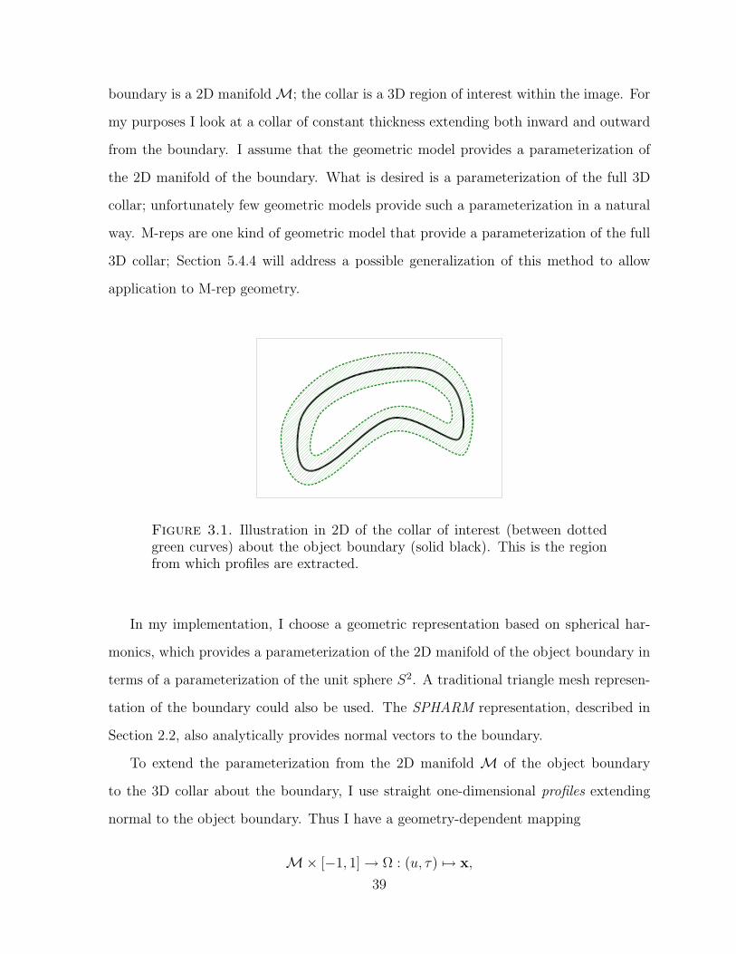
boundary is a 2D manifold M; the collar is a 3D region of interest within the image. For

my purposes I look at a collar of constant thickness extending both inward and outward

from the boundary. I assume that the geometric model provides a parameterization of

the 2D manifold of the boundary. What is desired is a parameterization of the full 3D

collar; unfortunately few geometric models provide such a parameterization in a natural

way. M-reps are one kind of geometric model that provide a parameterization of the full

3D collar; Section 5.4.4 will address a possible generalization of this method to allow

application to M-rep geometry.

Figure 3.1. Illustration in 2D of the collar of interest (between dottedgreen curves) about the object boundary (solid black). This is the regionfrom which profiles are extracted.

In my implementation, I choose a geometric representation based on spherical har-

monics, which provides a parameterization of the 2D manifold of the object boundary in

terms of a parameterization of the unit sphere S2. A traditional triangle mesh represen-

tation of the boundary could also be used. The SPHARM representation, described in

Section 2.2, also analytically provides normal vectors to the boundary.

To extend the parameterization from the 2D manifold M of the object boundary

to the 3D collar about the boundary, I use straight one-dimensional profiles extending

normal to the object boundary. Thus I have a geometry-dependent mapping

M× [−1, 1] → Ω : (u, τ) 7→ x,

39

where u parameterizes the object boundary, τ specifies distance normal to the boundary,

and x represents a location in the original (x, y, z) image coordinates. Since M is a 2D

manifold, u is a parameter vector with two degrees of freedom. The units of τ need not be

Euclidean distance, but in my implementation the sampling along each profile is uniform

in Euclidean distance. This definition of profiles uses a local linear approximation to

the object boundary M to estimate a parameterization of the entire collar about the

object boundary. This is the standard profile sampling scheme used by Active Shape

Models [Cootes et al. 1993] and Kelemen’s SPHARM segmentation framework. This is

what I use in my implemention as well. Where the manifold M has curvature, however,

the straight-line profiles may cross. Possible future work could be to refine the profile

sampling scheme, perhaps by a flow-field away from M along the distance map. If

the object geometry is represented by m-reps [Pizer et al. 2003] instead of SPHARMs,

then another parameterization can be provided of a collar about the object. Profiles from

such parameterizations would no longer be straight, and might be sampled non-uniformly

along their lengths.

Given a parameterization of the collar about the object boundary, I sample a pro-

file image I from the original image on profiles across the object boundary. With the

SPHARM geometric representation, the parameter space of the spherical harmonics is

the surface of the unit sphere, S2. Hence a natural space for the normalized coordinate

system is

(θ, φ, τ) ∈ S2 × [−1, 1]

where (θ, φ) parameterize the sphere and τ indicates distance normal to the boundary.

This is a spherical shell with thickness; it represents an idealized collar about the object

boundary. Normals on the sphere S2 map to normals on the object boundary M; the

collar has constant thickness in the image space.

The profile image I is a scalar function on the normalized coordinate space:

I : M× [−1, 1] → R.

40

For my purposes, I can also consider the profile image I as a tuple-valued function defined

on the surface of the unit sphere:

I : S2 → L2[−1, 1],

where the value of I at each (θ, φ) on the sphere is a 1D function describing the intensity

profile across the object boundary at that point. A possible extension could represent

the 1D profiles via orthogonal polynomial expansion, e.g., Legendre polynomials.

A uniform sampling of the object boundary is obtained by an octahedron-based tri-

angle subdivision of the sphere S2. At each point on the object boundary, the image

is sampled evenly along a straight line normal to the boundary, producing an image

profile. The first image in Figure 3.2 shows 512 profiles taken around one caudate from

the training set. The 1D ordering of the profiles represents a certain traversal of the 2D

surface of the object; adjacent profiles in this visualization are not necessarily adjacent

on the surface. This visualization does illustrate the complex image appearance at the

boundary: some profiles show the border with the ventricle (black in T1-weighted MRI),

some show a border with white matter, and some show no contrast at all with tissue

outside the caudate.

Figure 3.2. Intensity profiles from the boundary of a single caudate. Atleft is a linear visualization of the profiles: the left half is inside the caudate;the right half is outside. At right is an “onionskin” visualization of theprofiles mapped onto concentric spheres. Each sphere represents sampledintensities at a fixed distance away from the boundary, from -5mm to+5mm, with 1mm spacing.

41

The right image in Figure 3.2 shows a different visualization of the same profiles,

mapped onto concentric spheres. The diffeomorphic mapping of the object to the sphere

S2 provided by the shape representation is used to map each level of the profiles to a

sphere. The outermost sphere represents intensities sampled from an “onionskin” +5mm

outside the object boundary. Each profile is 11 samples long, so there are 11 concentric

spheres in the visualization. The uniform grey matter interior of the caudate can be seen

on the interior spheres.

Figure 3.3 shows one particular “onionskin” at +5mm outside one particular caudate.

The image intensities are texture-mapped back onto the geometry of the caudate at the

boundary, as defined by the manual expert segmentation. Four levels of scale are shown

to illustrate the scale space along the boundary.

42

(a) (b)

(c) (d)

Figure 3.3. Visualization of an “onionskin” sampled at +5mm outsidethe caudate, texture-mapped back onto the original caudate geometry(manual expert segmentation). Shown are four scale levels from the scalespace, fine to coarse. The region abutting the lateral ventricle (see Fig-ure 1.4) is seen as a medium-large scale dark area.

43

3.2. The Probabilistic Model on the Profile Scale Space

The preceding section defined a profile scale space, a scale space on a set of profiles

taken about the boundary of a single geometric object in a single image. In this section

I define my Bayesian image match model as a particular probability distribution on the

profile scale space.

A Bayesian image match model for deformable-models segmentation is a probability

distribution on features obtained from an image, given an instance of object geometry.

Image match models are trained by extracting features from a population of training

images that each have corresponding object geometry from expert segmentation.

My project uses a population of 114 magnetic resonance images (MRIs) of the human

brain with corresponding manual segmentations of the caudate provided by human expert

raters (see Section 4.2 for more details). My image match model is trained by first

building a profile scale space for each image in the training population, using geometry

from the corresponding manual segmentation. Each profile scale space in the training

population is then sampled to obtain a collection of profiles blurred at multiple scales; this

is described in Section 3.2.1 The blurred profiles are used to train the Markov Random

Field (MRF) probability distribution that defines my image match model; Section 3.2.2

discusses this MRF model.

There may be other ways to define a probability distribution on a scale space; the

approach I choose is inspired by multiresolution Markov Random Fields on 2D im-

ages [Bouman and Shapiro 1994, Willsky 2002].

3.2.1. Sampling the Profile Scale Space. A profile scale space Φ(f) as described in

Section 3.1 can be seen as a tuple-valued function on the domain S2×R+. At each point

(φ, θ) in the parameter space S2 of the SPHARM geometric representation of the object,

for each scale σ in R+, the tuple given by Φ(f)(φ, θ; σ) represents a blurred profile of

the object boundary at the point mapped to by (φ, θ), blurred at scale σ. The profile

scale space is continuous, but in order to develop a probabilistic model I sample from the

continuous profile scale space at a discrete set of (φ, θ) and σ. Following the concept of

44

the Gaussian pyramid for images in Euclidean space, I sample the parameter space S2

more sparsely at coarser scales and more densely at finer scales.

My sampling of S2 is derived from a triangular tessellation of the sphere. I start with

an octahedron; the center of each of the eight triangles corresponds to a coarse-scale

blurred profile. A recursive triangle subdivision provides denser samplings of the sphere,

at which finer-scale profiles are sampled from the continuous profile scale space. I use

512 profiles at the finest scale, 128 profiles at a coarser scale, 32 profiles at a yet coarser

scale, and 8 profiles at the top level of scale. The recursive triangle subdivision also

provides parent-child relationships between profiles at adjacent scales. A schematic of

the sampling scheme is illustrated in Figure 3.4(a). Each node in the tree graph (call it

G) represents a single profile sampled from the profile scale space. The node at the top

of the tree represents a single coarse-scale profile summarizing an eighth of the boundary.

The figure only shows a portion of the sampling for clarity, but the hierarchical sampling

is on the whole sphere S2.

(a) (b)

Figure 3.4. (a) Visualization of the coarse-to-fine sampling of the profilescale space. Each node in the tree G represents a single profile sampledfrom the profile scale space. Distance away from the grey sphere indicatescoarser scale in the scale space. (b) Average profiles across the trainingpopulation, at four scales, fine to coarse.

These blurred profiles are calculated for each object in the training population. To

visualize the sampled profiles, Figure 3.4(b) shows the mean profiles at multiple scales,

where the mean is taken at corresponding locations over the training population. Cor-

respondence is established via the spherical harmonic parameterization [Kelemen et al.

45

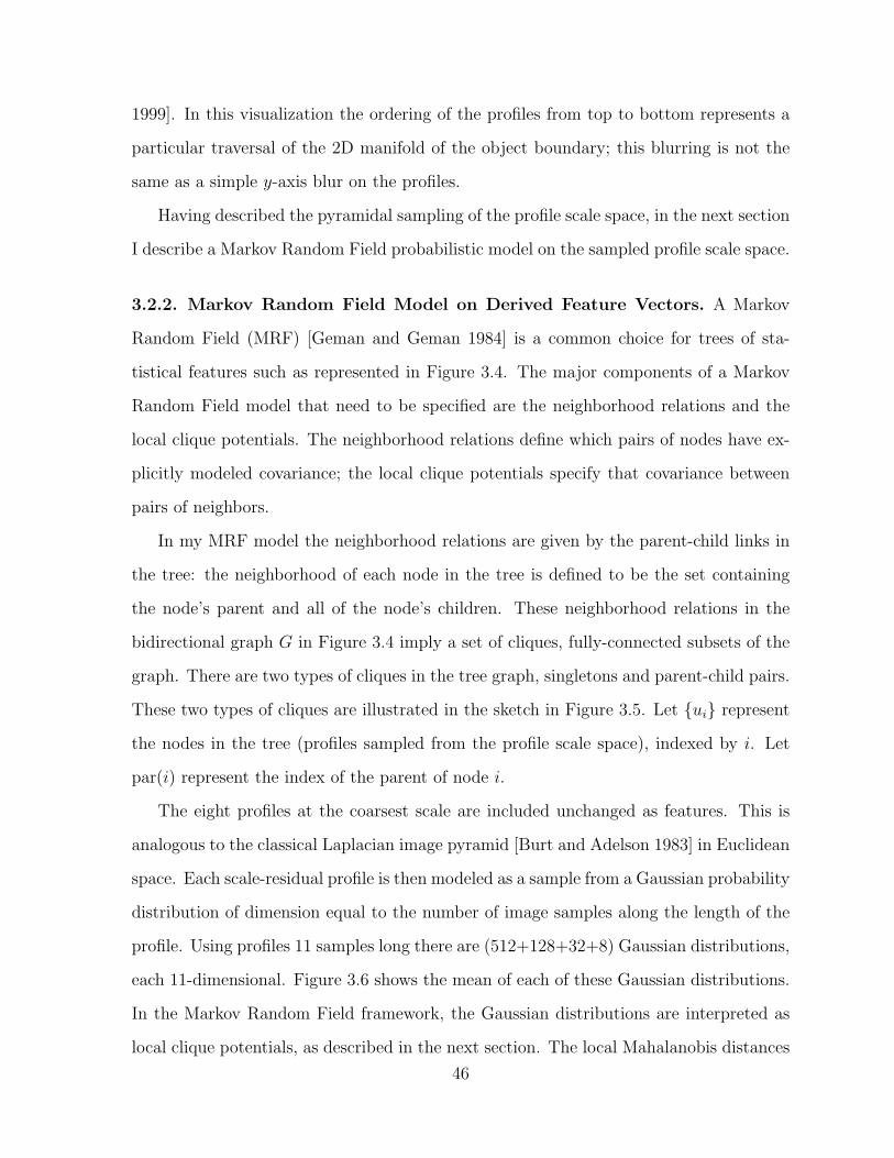
1999]. In this visualization the ordering of the profiles from top to bottom represents a

particular traversal of the 2D manifold of the object boundary; this blurring is not the

same as a simple y-axis blur on the profiles.

Having described the pyramidal sampling of the profile scale space, in the next section

I describe a Markov Random Field probabilistic model on the sampled profile scale space.

3.2.2. Markov Random Field Model on Derived Feature Vectors. A Markov

Random Field (MRF) [Geman and Geman 1984] is a common choice for trees of sta-

tistical features such as represented in Figure 3.4. The major components of a Markov

Random Field model that need to be specified are the neighborhood relations and the

local clique potentials. The neighborhood relations define which pairs of nodes have ex-

plicitly modeled covariance; the local clique potentials specify that covariance between

pairs of neighbors.

In my MRF model the neighborhood relations are given by the parent-child links in

the tree: the neighborhood of each node in the tree is defined to be the set containing

the node’s parent and all of the node’s children. These neighborhood relations in the

bidirectional graph G in Figure 3.4 imply a set of cliques, fully-connected subsets of the

graph. There are two types of cliques in the tree graph, singletons and parent-child pairs.

These two types of cliques are illustrated in the sketch in Figure 3.5. Let ui represent

the nodes in the tree (profiles sampled from the profile scale space), indexed by i. Let

par(i) represent the index of the parent of node i.

The eight profiles at the coarsest scale are included unchanged as features. This is

analogous to the classical Laplacian image pyramid [Burt and Adelson 1983] in Euclidean

space. Each scale-residual profile is then modeled as a sample from a Gaussian probability

distribution of dimension equal to the number of image samples along the length of the

profile. Using profiles 11 samples long there are (512+128+32+8) Gaussian distributions,

each 11-dimensional. Figure 3.6 shows the mean of each of these Gaussian distributions.

In the Markov Random Field framework, the Gaussian distributions are interpreted as

local clique potentials, as described in the next section. The local Mahalanobis distances

46

Figure 3.5. Sketch of two types of cliques in a Markov Random Fieldgraph. Singletons (circles) are cliques of only one node. Parent-child pairs(dashed ovals) are cliques of two nodes.

are summed to produce a global image match. Compare this model with a single-scale

profile model akin to that used in Active Shape Models, which would have 512 Gaussians,

each 11-dimensional. Compare also to Active Appearance Models, which would have a

single very high-dimensional Gaussian rather than many low-dimensional Gaussians.

Figure 3.6. Means of scale residuals from the profile scale space. Fourscale levels are shown, fine to coarse (the coarsest level of scale does notrepresent scale residuals but original blurred profiles). Each row in eachscale level represents the mean of a local Gaussian potential.

Thus the multiscale features used are samples from a Laplacian pyramid on the ob-

ject boundary M, akin to Laplacian basis functions, except that the domain is no longer

Euclidean space but the manifold of the object boundary. Rather than a Laplacian basis,

it is possible to use an orthogonal set of wavelet bases [Van de Wouwer 1998]; this has

47

been done by others in Euclidean space to produce wavelet-domain hidden Markov mod-

els [Choi and Baraniuk 2001, Liu et al. 1999]. In this domain spherical wavelets [Schroder

and Sweldens 1995] may be appropriate.

3.2.2.1. Local Clique Potentials. To specify the MRF model, local potential functions

need to be defined for each clique in the tree of features. For the singleton cliques

the local potentials are in the form V si(ui). For the singletons at the coarsest level of

scale (8 profiles in my sampling) I choose to measure the Mahalanobis distance in a

multidimensional Gaussian:

Vi(ui) = Mahalanobisµi,Σi(ui)(65)

= (ui − µi)T Σi (ui − µi) .(66)

The finer-scale singeltons are modeled with constant potentials and do not contribute

directly to the overall probability distribution. The tilde superscripts denote parameters

related to the singleton cliques.

For parent-child pairs (ui, upar(i)) I define the clique potential to be a Mahalanobis

distance on the difference or residual between a node and its parent:

Vi(ui, upar(i)) = Mahalanobisµi,Σi(ui − upar(i))(67)

=(ui − upar(i) − µi

)TΣi

(ui − upar(i) − µi

).(68)

I define the local clique potentials using Gaussians, but other choices of clique poten-

tial could also be used.

3.2.2.2. Markov Assumption. The Markov assumption on the derived feature vectors u

with respect to the tree G is that the conditional likelihood of any feature vector given

all the other feature vectors in the tree is the same as the conditional likelihood of that

feature vector given only its parent:

p (ui|uj : j 6= i) = p(ui|upar(i)

).

48

3.2.2.3. Gibbs formulation. According to the Hammersley-Clifford theorem [Hammers-

ley and Clifford 1972, Geman and Geman 1984] making the Markov assumption on u

with respect to the tree G is equivalent to modeling the distribution p(u) with a Gibbs

distribution:

(69) p(u) =1

Ze−

1T (

∑i Vi+

∑i Vi),

where Z is a normalization factor (partition function) and T is a constant (temperature).

This defines a probability distribution on the feature vectors u = ui derived from the

profile image I. The profile image samples the image relative to the boundary given by

the geometric shape representation. The likelihood p(u) defines the image match p(I|m),

how well a deformed shape model matches the image.

Compare this formulation of p(I|m) to that used by the classical single-scale profile

model:

(70) p′(I|m) =1

Z ′e−

∑j V ′

j ,

where the index j iterates over all profiles around the boundary, and the local Gaussian

potentials V ′j are on individual profiles, estimated by conditional maximum likelihood

estimation. Z ′ is the normalization factor for the single-scale image match.

Both my multiscale profile model and the single-scale profile model make assump-

tions on the interdependence between profiles. In the single-scale model, each profile

is assumed to be independent of all other profiles: the overall image match is simply

the product of the Gaussian likelihoods for individual profiles. In my multiscale profile

model, dependence between profiles is modeled. The Markov assumption I use states

that the interdependence of profiles is only through the parents in scale in the graph G.

3.2.3. Parameter Estimation. The parameters in the Gibbs distribution p(u) are the

vectors and matrices for each of the Gaussian local clique potentials: µi, Σi, µi, Σi for each

clique. The “temperature” T is a user-adjustable parameter. The normalization factor

(partition function) Z can be derived from the Σi and Σi.

49

Since each of the local clique potentials is merely a quadratic, a conditional max-

imum likelihood estimate of each (µi, Σi) and (µi, Σi) is straightforward. From each

segmented image in the training population the profile scale space is built and sampled

to get the feature vectors uni , where i indexes position and scale in the scale space and

n ∈ [1, N ] indexes the case number in the training population. The scale residuals are

uni − un

par(i). Then the conditional maximum likelihood estimates of the parameters

in the local Gaussian potentials can be made in the usual way, e.g., via singular value

decomposition:

µi =1

N

∑n=1

Nuni ,(71)

µi =1

N

∑n=1

Nuni − un

par(i),(72)

Σi(n1, n2) = (un1i − µi)

T (un2i − µi) ,(73)

Σi(n1, n2) =(un1

i − un1

par(i) − µi

)T (un2

i − un2

par(i) − µi

).(74)

Σi(n1, n2) denotes the (n1, n2)-th element of the covariance matrix Σi.

However, the true maximum likelihood estimate of the parameters requires an esti-

mate of all the (µi, Σi) simultaneously. A computationally expensive iterative method

of finding the true maximum likelihood estimate is the Monte Carlo Markov Chain

(MCMC) [Doucet 1998] method, which converges in the limit. The conditional maxi-

mum likelihood estimate, however, is a reasonable estimate that is easily computed and

can be used as an intialization for further MCMC refinement if desired.

50

CHAPTER 4

Experimental Results

Chapter 3 defined the new multiscale profile model that I use for image match in

Bayesian segmentation. In this chapter I describe validation experiments which measure

the quality and efficacy of my multiscale profile model in comparison with the classical

single-scale profile model used in Active Shape Models and Kelemen’s SPHARM segmen-

tation framework. Section 4.1 describes the Mathematica implementation I have written

of both my new multiscale profile model and the classical single-scale profile model. A

segmentation framework has also been implemented to optimize the image match from

the profile models together with a shape prior. Section 4.2 discusses the 114 magnetic

resonance image (MRI) datasets I use and their associated high-quality manual segmenta-

tions of the caudate. These are the images I use for training my profile model, validating

it, and evaluating its efficacy in segmentation. In Section 4.3.1 my multiscale profile

model is compared against the single-scale profile model in the areas of model generaliz-

ability, specificity, and variance. Section 4.3.2 evaluates the performance of both profile

models in segmentation, using the same shape prior for both image match models.

4.1. Implementation

A complete model-building and segmentation framework to test the methods pre-

sented in Chapter 3 has been written in Mathematica, as a proof-of-concept implementa-

tion. Mathematica notebooks have been written to build the SPHARM statistical shape

model and my new multiscale profile model. Notebooks have also been provided to use

these models in segmentation. A single-scale profile model in the fashion of Kelemen’s

SPHARM segmentation framework has also been provided for comparison. The segmen-

tation process uses exactly the same shape prior with both multiscale and single-scale

profile models, to facilitate comparison of the two image match models.

The implementation expects as input the population of training images in the Hier-

archical Data Format (HDF) file format. External C programs are needed to preprocess

the binary segmentation label-map images, extracting a surface net representation of the

segmentation, as well as the area-preserving parameterization in S2 of the object surface.

From the *.net surface net files and the *.par parameterizations of the object sur-

face, the Mathematica notebooks can extract SPHARM representations of the segmented

objects.

The package is a set of over a dozen Mathematica 5.0 notebooks, including the fol-

lowing:

ExtractSpharm.nb: Calculates SPHARM geometric representations of the seg-

mented objects from *.net and *.par files.

ShapeModel.nb: Builds the SPHARM statistical shape model.

SampleImage.nb: Samples profiles from the training images relative to their seg-

mentations.

SmoothTextures.nb: Builds the profile scale space as defined in Section 3.1.6.

ProfileModel.nb: Builds the new multiscale profile model for statistical image

match.

ProfileModelASM.nb: Builds the classical single-scale profile model, for compar-

ison.

Segmenter.nb: Segments a target image using the SPHARM statistical shape

prior and either my new multiscale image match or the classical single-scale

image match.

More detailed implementation notes can be found in the Mathematica notebooks,

which allow both documentation and implementation to be interwoven in a logical outline

format.

52

Figure 4.1. Illustration of the deformable segmentation process, showinginitialization (mean shape) in red and manual “gold standard” segmenta-tion in yellow.

4.1.1. Single-scale Profile Model. The single-scale profile model is implemented in

the notebooks SampleImage.nb and ProfileModelASM.nb. Each training image has an

associated SPHARM shape representing its manual segmentation (see Section 4.2 below

for more details). Subroutines in SampleImage.nb sample the image along 512 equally-

spaced straight-line profiles normal to the object boundary; each profile has 11 samples

along its length at 1mm spacing. Half of the samples are inside, and half are outside the

object. This is done for each of the images in the training population; the profiles are

then saved to disk.

The notebook ProfileModelASM.nb produces for each of the 512 profiles a separate

11-dimensional Gaussian model at that location on the object boundary. The overall

image match across all profiles is defined to be the product of all the 512 individual

Gaussian likelihoods, as described in Section 3.2.2.3.

The single-scale profile model is designed to be modular with the new multiscale

profile model, such that in segmentation a simple “switch” toggles between the two

profile models, while using the same shape prior.

4.1.2. Multiscale extension. To implement my new multiscale profile model, for each

training image, I start from the 512 profiles of length 11 obtained by SampleImage.nb,

and treat them as 11 different textures (scalar-valued functions) on the corresponding

SPHARM shape. The SPHARM shape representation allows one to think of the 11

53

“onionskin” textures as scalar-valued functions on the sphere, the parameter space of

the SPHARMs. To construct the scale space as defined in Section 3.1.2, I use the same

subroutines that were used to extract coefficients of spherical harmonics for the shape

representation; they are reused to obtain coefficients of spherical harmonics for repre-

sentation of the image profiles, one “onionskin” at a time. Reconstruction of a blurred

version of a texture is then simply an interpolation with spherical harmonics, modulated

by the e−l(l+1)t factor as discussed in Section 3.1.2.

In my implementation I sample the profile scale space at four levels of scale, following

a coarse-to-fine pyramidal sampling from the octahedron-based triangle subdivision of

the sphere. At the finest level of scale there are 512 profiles; the coarser levels have 128,

32, and finally 8 profiles. Thus at the coarsest level of scale each profile sampled from

the scale space represents one octant of the object boundary. The feature vectors used

in the Markov Random Field probabilistic model are the scale residuals ui − upar(i);

these are obtained simply enough, since the triangle subdivision of the sphere allows me

to keep track of “parent” triangles and hence “parent” nodes in the scale space. The 8

profiles at the top coarsest level of scale are used as-is.

Conditional maximum-likelihood parameter estimation is performed for each of the

512+128+32+8 local potentials, by calculating mean and covariance matrices on the

scale-residual profiles (in the case of the 3 finer scales) or on the blurred profiles (in the

case of the top level of scale). The normalization factor Z (“partition function”) in the

Gibbs distribution (see Section 3.2.2.3) is not explicitly calculated. The optimization for

segmentation, described in the next section, minimizes − log p(I|m). Since p(I|m) is in

the form of a Gibbs distribution,

− log p(I|m) = − log1

Ze−

1T (

∑i Vi+

∑i Vi)(75)

= log Z +1

T

(∑i

Vi +∑

i

Vi

).(76)

54

The log Z term is fixed once the model has been trained, so it can be ignored in the

optimization process. The 1/T factor can be absorbed in a user-controlled parameter

determining the relative weights of the shape prior versus the image match.

4.1.3. Shape Prior. The shape prior I use is a Gaussian distribution on the spherical

harmonic coefficients of shape, the same as that used in Kelemen’s SPHARM segmenta-

tion framework:

p(m) = N(µc, Σc)(c)(77)

=1

Zc

e−12(c−µc)T Σc(c−µc),(78)

where N(µc, Σc)(c) represents the Gaussian likelihood of the coefficient set c in the

multidimensional normal distribution with mean shape µc and covariance matrix Σc. Zc

is a normalization factor. The parameters µc and Σc of the Gaussian distribution are

trained on a training set of shapes from manual segmentation, normalized for translation

and rotation.

4.1.4. Optimization. With the probabilistic models for shape prior and image match

likelihood defined Bayesian segmentation is simply optimization of the posterior, equiv-

alent to minimization of the sum − log p(m) − log p(I|m). The optimization is easy

to specify but difficult to implement in a robust and efficient way. Mathematica pro-

vides a number of sophisticated optimization libraries, including non-linear optimization

via genetic algorithms (DifferentialEvolution), simplex (NelderMead), and random-

ized local search (RandomSearch). During development of my implementation various

optimization techniques were tried, but the numerous program parameters in the non-

linear techniques proved too complex to fine-tune to gain an understanding of what the

optimization was doing “behind the scenes”. For the segmentation results shown in Sec-

tion 4.3.2 simple conjugate-gradient optimization (FindMinimum) is used. Initialization

is always at the mean shape; mean translation and rotation is also recorded and used for

pose initialization. A hyper-parameter β modulates the log-likelihood of image match:

55

β log p(I|m). This allows the user to shift the weighting between shape prior and image

match. The default value of β is 0.05 and is fixed for both multiscale and single-scale

image match models.

Since the optimization is searching for the best shape to fit the image, the search space

over which optimization is performed is the shape space. The shape space is limited to

the 12 largest eigenmodes of deformation. The geometric representation also allows

unrestricted motion of the object in translation and rotation; the total dimension of the

search space is 18. Thus the search space is not too large, but each iteration takes about

6-7 seconds on a 2GHz Intel Xeon server with 2GB of RAM. About half the time is spent

building and sampling from the profile scale space.

4.2. Image Datasets and Manual Segmentations

This project is fortunate in that access is provided to an unusually large and high-

quality set of segmented images. A total of 115 high-resolution images with high-quality

expert manual segmentations of the caudate have been provided by two projects in the

Psychiatry department at UNC: a longitudinal study in autism (NIH RO1 MH61696)

and a longitudinal study in Fragile X syndrome (NIMH MH 64580); Dr. Joseph Piven

is the principal investigator of both. Manual segmentations are by Michael Graves, with

protocol development by Rachel Gimpel and Heather Cody Hazlett. Image processing is

by Rachel Gimpel.

The grayscale images are mostly coronal IRPrep T1-weighted MRI, with voxel sizes of

0.78125×0.78125×1.5mm3 and resolution 256×256×124. Each was then rigidly aligned

to a Talairach coordinate system via AC/PC landmarks and resampled to 1× 1× 1mm3

voxel spacing. For processing efficiency I cropped a fixed region of interest about the

caudate and converted to the HDF image file format for import into Mathematica. No

intensity normalization was performed on the images; the MR images in this study are

quite consistent in global brightness and contrast. My multiscale profile model isolates the

global brightness level (i.e., additive constant) in the top (coarsest) level of the pyramid

56

sampled from the profile scale space. Since the features at finer levels of scale are all

scale residuals, they are inherently normalized for global brightness. Contrast (i.e., a

multiplicative constant) which is consistent across the population is modeled in the local

covariance matrices.

Figure 4.2. Cropped axial view of the caudate in T1-weighted MRI. Thedark butterfly shape in the upper center of the image is the lateral ventri-cles; the left and right caudates are the two gray blobby structures boundedby the “wings” of the butterfly.

For the Psychiatry projects the manual raters spent a number of months developing

a very careful protocol for manual segmentation of the caudate; as a result, the manual

“gold-standard” segmentations are of high quality. A subset of the images was manually

segmented repeatedly; I use these repeated segmentations to evaluate inter-rater and

intra-rater reliability in the manual segmentation. Five datasets were chosen from the

pool of images, replicated three times, and randomly ordered. Two experts then manually

segmented each of the 15 3D images, resulting in a total of six segmentations for each of

the five datasets. The self-consistency of each expert can be evaluated, since each expert

segmented each image three times. The two experts can also be compared, to see if they

do the same job. It is rare in medical image analysis to have these figures for the manual

raters; it allows evaluation of the reliability of my automatic segmentation method in the

context of the reliability of manual experts.

The manual segmentation reliability study will be discussed again in the segmentation

tests in Section 4.3.2. The next section first evaluates my multiscale profile model on its

57

own as a probabilistic model, separate from a segmentation framework; evaluation of my

profile model for use in segmentation is discussed later.

58

4.3. Validation

In this section I compare my new multiscale profile model to a standard single-scale

profile model, akin to that used by Active Shape Models or the spherical harmonics

framework of [Kelemen et al. 1999]. Validation is done in two parts: first, the profile

model is be evaluated on its own as a probabilistic model – how well does the model

fit the training data? Secondly, the profile model can be evaluated for its utility in

segmentation – does it contribute towards automatic segmentations that are closer to

the manual segmentations?

4.3.1. Evaluation of the Probabilistic Model. An image match model can be eval-

uated as a probabilistic model on a high-dimensional feature space: given a training

population, one can ask how well the model fits the training population. Two aspects

of model quality that are of interest are generalizability and specificity. Generalizability

is a measure of how well the model generalizes to a sample point outside the training

population. Specificity is a measure of how tightly the model fits around the training

population. I evaluate generalizability by using a sample from the random variable which

is not part of the training population. The likelihood of that sample in the probability

distribution yields a measure of generalizability. To evaluate specificity, I use a random

sample generated from the probability distribution. The distance from that generated

sample to the nearest sample in the training population yields a measure of specificity.

This requires a distance metric between samples of the random variable. In Section 4.3.1.3

I also evaluate the variance of the single-scale and multiscale profile models.

Figure 4.3 illustrates generalizability and specificity using a toy example in a 1D

feature space. The x axis indicates the value of a single random variable; round dots are

values of the random variable in a training population. The y axis indicates probability

density in the model; the probability distribution is shown as a curve. The “X” indicates

the value of a sample which was not included in the training, but which comes from the

same random variable and ought to have a high likelihood in the model. Figure 4.3(a)

shows a model that is quite general but not very specific. Although it gives a high

59

likelihood to the left-out sample point “X”, the model is likely to generate samples which

are very far from the training population. Figure 4.3(b) illustrates the other extreme:

the model is very specific to the training population (generated samples are likely to be

very near the training population), but the model does not generalize well to the sample

point “X”, which ought to have a high likelihood. Figure 4.3(c) shows one possible

model that strikes a balance between generalizability and specificity. The models in

these sketches were in fact generated by Gaussian Parzen windowing with window sizes

of σ = 0.8, 0.02, 0.09.

(a) (b) (c)

Figure 4.3. Illustration of generalizability and specificity in model qual-ity, using a toy example in 1D. x axis is the value of the random variable;y axis is probability. (a) The model (curve) is very general but not veryspecific to the training population (round dots). (b) The model is veryspecific to the training, but does not generalize well to the new samplepoint marked with an “X”. (c) The model balances generalizability withspecificity.

Styner et al have used the concepts of generalizability and specificity in comparing

various definitions of point-to-point correspondence in shape representation [Styner et al.

2003]. I also examine variance in the image match models, since the models use Gaussian

distributions.

I examine the quality of the model as a function of training population size; the

claim is that my new multiscale profile model requires fewer training samples to obtain

a “good” model than the classical single-scale profile model does. There is a fixed total

of 114 segmented images, from which profiles can be extracted relative to the manually

segmented objects. I consider five sizes of training populations, using 10%, 30%, 50%,

70%, and 90% of the total pool of images to train the model. For each size I randomly

selected training populations five times from the total pool, training a model on each of

60

those populations. Thus the model was trained a total of 25 times on different popula-

tions. For each choice of training population the remaining images from the pool of 114

can be used as test images. This is a series of jack-knife tests, splitting the total pool at

random into training and testing populations.

4.3.1.1. Generalizability. To evaluate generalizability, for each split of training versus

testing populations, the model is trained on the training population and the likelihood

of each sample in the testing population is evaluated. If the model is generalizable, then

the generated samples should have high likelihood in the model. The results can be

considered for the various sizes of training population.

Figure 4.4 shows the likelihood of samples from the testing populations, for various

sizes of training population. Each column of dots represents one choice of test vs. training

and hence one instance of a trained model. The columns are clustered according to size

of training population, at 10%, 30%, 50%, 70%, and 90% of the total of 114 segmented

images. The vertical axis indicates the negative log-likelihood of each of 5 test samples

in each of the trained instances of the model; lower values are increased likelihood and

better generalizability of the model.

(a) (b)

Figure 4.4. Generalizability of (a) the multiscale profile model and (b)the single-scale profile model, as a function of training population size.Training populations are chosen of sizes 10%, 30%, 50%, 70%, and 90% ofthe total pool of 114. For each size, five training populations were randomlyselected; the remainder were used for testing. For each trained model, thelikelihood of the test samples are plotted in the vertical axis; higher valuesindicate better generalizability.

61

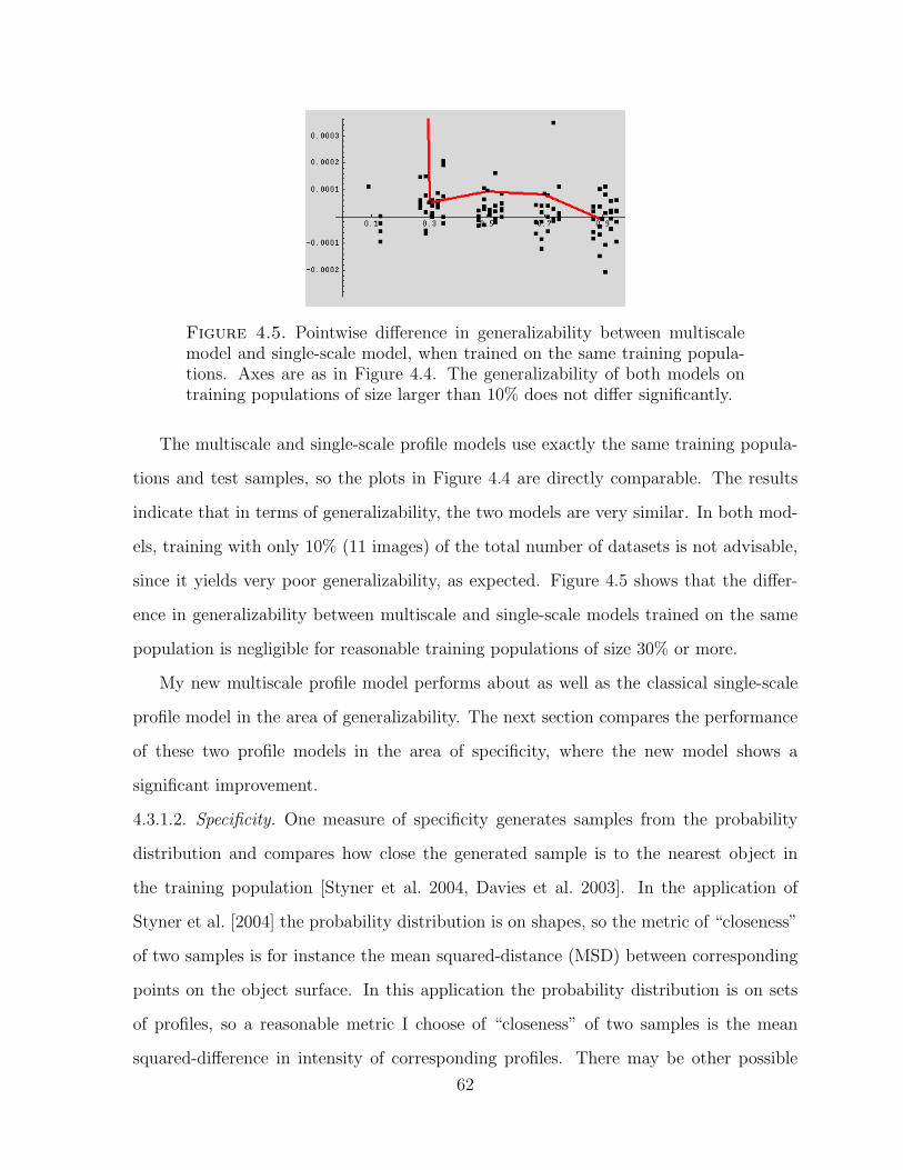
Figure 4.5. Pointwise difference in generalizability between multiscalemodel and single-scale model, when trained on the same training popula-tions. Axes are as in Figure 4.4. The generalizability of both models ontraining populations of size larger than 10% does not differ significantly.

The multiscale and single-scale profile models use exactly the same training popula-

tions and test samples, so the plots in Figure 4.4 are directly comparable. The results

indicate that in terms of generalizability, the two models are very similar. In both mod-

els, training with only 10% (11 images) of the total number of datasets is not advisable,

since it yields very poor generalizability, as expected. Figure 4.5 shows that the differ-

ence in generalizability between multiscale and single-scale models trained on the same

population is negligible for reasonable training populations of size 30% or more.

My new multiscale profile model performs about as well as the classical single-scale

profile model in the area of generalizability. The next section compares the performance

of these two profile models in the area of specificity, where the new model shows a

significant improvement.

4.3.1.2. Specificity. One measure of specificity generates samples from the probability

distribution and compares how close the generated sample is to the nearest object in

the training population [Styner et al. 2004, Davies et al. 2003]. In the application of

Styner et al. [2004] the probability distribution is on shapes, so the metric of “closeness”

of two samples is for instance the mean squared-distance (MSD) between corresponding

points on the object surface. In this application the probability distribution is on sets

of profiles, so a reasonable metric I choose of “closeness” of two samples is the mean

squared-difference in intensity of corresponding profiles. There may be other possible

62

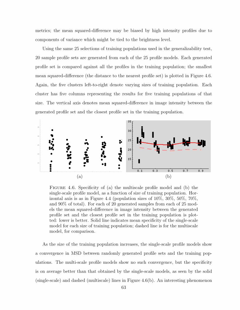
metrics; the mean squared-difference may be biased by high intensity profiles due to

components of variance which might be tied to the brightness level.

Using the same 25 selections of training populations used in the generalizability test,

20 sample profile sets are generated from each of the 25 profile models. Each generated

profile set is compared against all the profiles in the training population; the smallest

mean squared-difference (the distance to the nearest profile set) is plotted in Figure 4.6.

Again, the five clusters left-to-right denote varying sizes of training population. Each

cluster has five columns representing the results for five training populations of that

size. The vertical axis denotes mean squared-difference in image intensity between the

generated profile set and the closest profile set in the training population.

0.2 0.4 0.6 0.8 1

15

20

25

30

35

40

(a) (b)

Figure 4.6. Specificity of (a) the multiscale profile model and (b) thesingle-scale profile model, as a function of size of training population. Hor-izontal axis is as in Figure 4.4 (population sizes of 10%, 30%, 50%, 70%,and 90% of total). For each of 20 generated samples from each of 25 mod-els the mean squared-difference in image intensity between the generatedprofile set and the closest profile set in the training population is plot-ted: lower is better. Solid line indicates mean specificity of the single-scalemodel for each size of training population; dashed line is for the multiscalemodel, for comparison.

As the size of the training population increases, the single-scale profile models show

a convergence in MSD between randomly generated profile sets and the training pop-

ulations. The multi-scale profile models show no such convergence, but the specificity

is on average better than that obtained by the single-scale models, as seen by the solid

(single-scale) and dashed (multiscale) lines in Figure 4.6(b). An interesting phenomenon

63

is that, for a fixed training population, randomly generated samples from the multiscale

model lie within a wide range of distances from the training population, whereas ran-

domly generated samples from the single-scale model are all about the same distance

from the training population – the spread in specificity is tighter. One possible explana-

tion could be that the multiscale model has increased flexibility to reproduce small-scale

variability in the training population. The single-scale model may be consistent in the

sort of profiles it generates, but it may be unable to capture the small-scale variability

needed to come close to the individual training profiles.

Despite the difference in spread of specificity, my multi-scale model still shows signif-

icantly improved specificity over the single-scale profile model. Figure 4.3.1.2 shows the

p-value of a one-sided T-test comparing the distribution of specificity from the multiscale

model to the distribution from the single-scale model, using a pooled variance. This

hypothesis test is done separately for each of the 25 choices of training population; no

correction for multiple tests has been done.

Figure 4.7. Improvement in specificity using multiscale model, p-valuesp-values comparing specificity of the multiscale profile model with the single-scale

profile model, derived from data in Figure 4.6. Columns highlighted with blue arrowsare training populations that show a significant (p < 0.05) improvement in specificity in

the multiscale profile model over the standard single-scale model.

4.3.1.3. Variance. Since both the new multiscale profile model and the standard single-

scale profile model use Gaussians to represent local conditional probabilities, the variance

of these local Gaussians serves as a measure of how “tight” the distribution is. For a

unimodal distribution one would expect a high-specificity distribution to also exhibit

tight variance. In the single-scale case there are 512 Gaussian distributions, one for

64

each profile on the boundary. In the multiscale case there are 512+128+32+8 Gaussian

distributions, one for each location and scale according to the pyramidal sampling of

scale space. For each local Gaussian the variance is taken as the trace of the covariance

matrix (sum of eigenvalues). Figure 4.8(a) shows the sum of local variances for each of

the 25 multiscale profile models. Instead of a sum of the local variances, a weighted sum

could be used; however, the choice of weights is an open issue.

(a) (b)

Figure 4.8. Sum of local variance of (a) the multiscale profile modeland (b) the single-scale profile model, as a function of size of trainingpopulation. Axes are as in Figure 4.4.

Figure 4.8(b) shows the sum of local variances for each of the 25 single-scale pro-

file models. The overall shape of convergence is similar to the multiscale models, with

variance becoming more similar as training population size increases. This behavior is

to be expected since all the training populations draw from the same pool of 114 sub-

jects. However, note that the scale of the vertical axis in Figure 4.8(b) is twenty times

that of Figure 4.8(a). The multiscale profile models have more local Gaussian models

(512+128+32+8) than the single-scale models (512), and they have much lower variance,

indicating that they model the population more tightly.

There are multiple sources of noise and variability in the images. The blurring in my

multiscale profile model removes image noise which is independent of locality, thereby

lowering variance. Variability across different patients is not, however, reduced by blur-

ring in my multiscale model, since it only blurs within each image. My multiscale image

65

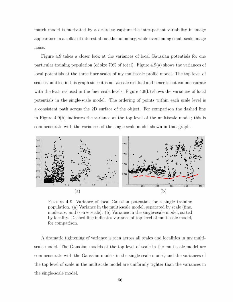
match model is motivated by a desire to capture the inter-patient variability in image

appearance in a collar of interest about the boundary, while overcoming small-scale image

noise.

Figure 4.9 takes a closer look at the variances of local Gaussian potentials for one

particular training population (of size 70% of total). Figure 4.9(a) shows the variances of

local potentials at the three finer scales of my multiscale profile model. The top level of

scale is omitted in this graph since it is not a scale residual and hence is not commensurate

with the features used in the finer scale levels. Figure 4.9(b) shows the variances of local

potentials in the single-scale model. The ordering of points within each scale level is

a consistent path across the 2D surface of the object. For comparison the dashed line

in Figure 4.9(b) indicates the variance at the top level of the multiscale model; this is

commensurate with the variances of the single-scale model shown in that graph.

(a) (b)

Figure 4.9. Variance of local Gaussian potentials for a single trainingpopulation. (a) Variance in the multi-scale model, separated by scale (fine,moderate, and coarse scale). (b) Variance in the single-scale model, sortedby locality. Dashed line indicates variance of top level of multiscale model,for comparison.

A dramatic tightening of variance is seen across all scales and localities in my multi-

scale model. The Gaussian models at the top level of scale in the multiscale model are

commensurate with the Gaussian models in the single-scale model, and the variances of

the top level of scale in the multiscale model are uniformly tighter than the variances in

the single-scale model.

66

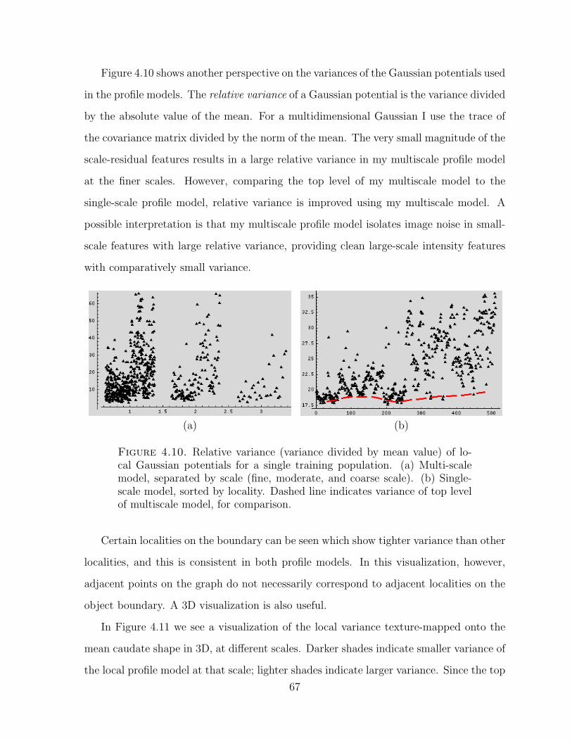
Figure 4.10 shows another perspective on the variances of the Gaussian potentials used

in the profile models. The relative variance of a Gaussian potential is the variance divided

by the absolute value of the mean. For a multidimensional Gaussian I use the trace of

the covariance matrix divided by the norm of the mean. The very small magnitude of the

scale-residual features results in a large relative variance in my multiscale profile model

at the finer scales. However, comparing the top level of my multiscale model to the

single-scale profile model, relative variance is improved using my multiscale model. A

possible interpretation is that my multiscale profile model isolates image noise in small-

scale features with large relative variance, providing clean large-scale intensity features

with comparatively small variance.

(a) (b)

Figure 4.10. Relative variance (variance divided by mean value) of lo-cal Gaussian potentials for a single training population. (a) Multi-scalemodel, separated by scale (fine, moderate, and coarse scale). (b) Single-scale model, sorted by locality. Dashed line indicates variance of top levelof multiscale model, for comparison.

Certain localities on the boundary can be seen which show tighter variance than other

localities, and this is consistent in both profile models. In this visualization, however,

adjacent points on the graph do not necessarily correspond to adjacent localities on the

object boundary. A 3D visualization is also useful.

In Figure 4.11 we see a visualization of the local variance texture-mapped onto the

mean caudate shape in 3D, at different scales. Darker shades indicate smaller variance of

the local profile model at that scale; lighter shades indicate larger variance. Since the top

67

level of scale does not model scale residuals (a la Laplacian pyramid) but blurred profiles

(a la Gaussian pyramid), the variance is much larger than it is for the scale residuals. The

variance of the scale residuals ranged from 7.7 to 1108; this is the range of the greyscale

colormap visualization in Figure 4.11. The variance at the top level of scale averaged

4746; it was omitted from the figure in order not to skew the colormap. This figure is for

one specific training population (the same as that used in Figure 4.9).

The visualization of local variance shows a patch midway near the tail of the caudate,

of medium scale (Figure 4.11(b)), which has larger variance than other locations at other

scales. The head of the caudate consistently abuts the lateral ventricle, but near the tail,

the caudate separates from the ventricle. Variability in the location of separation from

the ventricle results in variability in boundary profiles in that region; this may explain

the increased local variance at that patch.

From Figure 4.11 a summary figure can be produced: for each patch on the boundary,

an “optimal scale” for representation is selected, the scale at which the local variance is

smallest. The top level of scale is not included in this optimal scale selection, since it is not

commensurate with the other scales. Figure 4.12 shows the result, again texture-mapped

onto the mean caudate shape.

Evaluated as a probabilistic model, my new multiscale profile model shows signif-

icantly improved specificity and tighter variance compared to the classical single-scale

profile model. The validation study on generalizability shows that the two profile models

do not differ significantly in generalizability. Trends can also be seen as the training

population size is increased; both profile models improve with more training, particu-

larly in variance. The specificity of the single-scale profile model improves with larger

training populations, but the multiscale profile model consistently has signficantly better

specificity at all sizes of training population.

68

(a) (b)

(c)

Figure 4.11. Visualization of local variance in the multiscale profilemodel, with one training population. Dark indicates smaller variance; lightlarger variance (max 1108). Three scales are shown, from fine (a) to coarse(c). The colormap is the same for all three figures. A patch of mediumscale near the tail of the caudate has high variance; the caudate separatesfrom the ventricle near the tail, so the profiles are less consistent there.

69

Figure 4.12. Automatic selection of optimal scale for each patch on theboundary: each patch is shaded according to the scale at which variancein the profile model (trace of covariance matrix) is smallest. Three scalesare sampled from the scale space; darker is finer scale and brighter is coarserscale.

70

4.3.2. Evaluation in Segmentation. For each of the 25 divisions of the total popula-

tion into test-vs-training subsets, five test images are randomly selected for segmentation.

The implementation of the optimzation is as described in Section 4.1.4. Using the same

shape prior, the segmentation is run once (until a threshold of convergence is met) with

the new multiscale profile model and once with the standard single-scale profile model

for comparison. The resulting segmentations are then compared with the expert manual

segmentation of the test image.

Since the segmentations are run using the SPHARM shape representation, and I

also have SPHARM representations of the manual segmentations, it is straightforward

to calculate the mean squared-distance (MSD) between corresponding surface points.

This uses a convenient property of the spherical harmonic orthonormal decomposition of

shape, namely the Parseval equation:

(79)

∫S2

|x1(θ, φ)− x2(θ, φ)|2 ∝∞∑l=0

l∑m=−l

(c1ml − c2

ml )2,

where x1 and x2 are the (x, y, z) coordinates of surface points on the two shapes to

be compared and c1, c2 are the spherical harmonic coefficients of the respective shapes.

Hence the mean squared-distance between corresponding surface points can be obtained

directly from the SPHARM representations of the shapes. The MSD metric depends on

the point-to-point correspondence defined by the SPHARM shape representation. Other

shape difference metrics like volume overlap do not depend on correspondence, but they

may have other issues instead.

Figure 4.13 shows the automatic segmentation results, formatted in the same way as

the plots of model generalizability, variance, etc. The vertical axis indicates MSD in mm

from the manual segmentation. Figure 4.13(a) uses my new multiscale profile model for

image match; Figure 4.13(b) uses the classical single-scale profile model. The training

populations, shape prior, model initialization, and optimization scheme are identical in

both cases.

71

0.1 0.3 0.5 0.7 0.9Training Size

2

4

6

8

MSD

0.1 0.3 0.5 0.7 0.9Training Size

2

4

6

8

MSD

(a) (b)

Figure 4.13. Mean squared-distance between manual segmentation andautomatic segmentation using (a) multiscale and (b) single-scale profilemodel. Horizontal axis is as in Figure 4.4, vertical axis is mm of distance.

The results do not show a significant change in segmentation accuracy by using my

multiscale profile model instead of the classical single-scale profile model. Both automatic

segmentation methods are in these tests largely unable to come closer than 2mm in MSD

to the manual segmentations.

A major strength and motivation of scale-space representations is capturing moderate-

scale and coarse-scale structures of interest while overcoming small-scale noise. In the

high-resolution, high-quality, T1-weighted MRIs used in this study the signal-to-noise

ratio is very good. One possible explanation for why my multiscale profile model does

not show a significant improvement in segmentation is that the images are already “too

clean”, with insignificant small-scale noise. Figure 4.2 shows a slice through one of

the images used in this study. Future validation studies could evaluate segmentation

performance in the face of increasing amounts of artificially added image noise (e.g.,

Gaussian noise, independent at each voxel).

A complete automatic segmentation framework is much more than the image match

model; the interaction between the image match model and the shape prior is important,

as is the posterior optimization methodology. In my implementation I constructed the

log-posterior as a weighted sum of the log-prior and log-likelihood, and I used Mathemat-

ica’s conjugate-gradient optimizer as a “black-box” function to optimize the posterior.

72

However, poor control of the parameters of the optimizer may be biasing the results; the

effect could be greater than any improvement in segmentation provided by my multiscale

image match model.

Another factor in optimization is the parameter space over which optimization is per-

formed. To ease the optimization I chose the optimization space to be an 18-dimensional

space of 12 eigenloadings of shape deformation and 6 parameters for translation and ro-

tation. Thus the range of shapes produced by the automatic segmentation is limited to

the 12-dimensional subspace spanned by the 12 major modes of shape deformation. The

manually segmented shape is not limited to this 12-dimensional subspace; hence the au-

tomatic methods might not be able to come close to the manual segmentation, regardless

of which image match model is used. Future work to evaluate this hypothesis could use

the full 504-dimensional SPHARM shape space as the optimization space (while keep-

ing the same shape prior), or perhaps a final “lock-in” phase of segmentation where the

shape is allowed freely to deform without being constrained to the 12-dimensional shape

subspace.

The multiscale profile model also allows visualization of the image forces at work

during the segmentation, at various levels of scale. Figure 4.14 shows a snapshot of one

iteration of segmentation. The local image match (Mahalanobis distance) is shown for

each patch of the boundary, at three levels of scale. The lighter shading at the tail of

the caudate indicates worse fit; the visualizations also indicate that the fit is poor for a

large-scale portion of the boundary rather than for a small patch of it.

The local segmentation error can also be texture-mapped onto the object surface in

order to determine where the segmentation performed poorly and where it performed

better. Figure 4.15 shows a visualization of segmentation error on a single case after

many iterations of automatic segmentation using my multiscale image match model. The

shading at each point indicates point-to-point distance between corresponding points on

SPHARM representations of the automatic segmentation and a manual segmentation.

Darker shades represent lower distance (better segmentation); lighter shades indicate

73

Figure 4.14. Visualization of local image match of the geometry to onetarget image during an early iteration of segmentation, at three levels ofscale (coarse to fine). Light indicates worse fit, dark indicates better fit.The tail of the caudate has yet to fit into the image optimally at thisiteration.

larger distance (worse error). Interestingly enough the segmentation error seems to be

around the body of the caudate; the tail of the caudate is segmented to within 0.7mm

of the manual rater gold standard. That the segmentation errors are not uniformly

distributed over the surface indicates a systematic error; perhaps the automatic segmen-

tation was not given enough iterations to reach convergence, or perhaps the shape space

is excessively restrictive in allowable deformations.

4.3.2.1. Manual Rater Reliability. In this section I wish to evaluate the precision of the

manual segmentations that were used as gold standards for my automatic segmentation

schemes. I evaluate intra-rater and inter-rater reliability in manual segmentation for two

human raters (“Rater A” and “Rater B”) on a subset of images from the population.

A similar study using a volume overlap measure is discussed in [Joshi et al. 2004]. In

74

Figure 4.15. Visualization of local segmentation error after convergence.Darker shades indicate lower Euclidean distance to corresponding points onthe gold standard; lighter shades indicate larger error. This segmentationused my multiscale image match model; results with the single-scale profilemodel are similar.

my study SPHARM boundary representations were obtained for each of the manual

segmentations in the reliability study. Rather than volume overlap, the mean squared-

distance (MSD) between corresponding boundary points is used as the metric to compare

segmentations, to be consistent with the segmentation results presented in Figure 4.13.

Figure 4.16 shows average MSD for all pairs of segmentations for each of the five

datasets, categorized into intra-rater and inter-rater figures. For example each point in

the “Rater A” line represents three segmentations of each dataset; thus, there are three

pairs of segmentations to consider, and the height of a point on that line indicates the

average MSD across those three pairs. For the “A to B” column each dataset has three

segmentations by rater A and three segmentations by rater B. There are nine pairings

that compare A to B; the height of a point represents the average of those nine MSD of

pairs.

We see that the manual raters achieve a very high degree of reliability, with on aver-

age about 0.4mm in MSD between repeated segmentations. The expert raters invested

a number of months in developing a careful protocol for manual segmentation. In com-

parison neither of the automatic methods come within 2mm in MSD to the manual

segmentation standard.

75

Figure 4.16. Intra-rater (“Rater A” and “Rater B”) and inter-rater (“Ato B”) reliability for manual segmentation of five images, each repeatedthree times, by two expert raters (“Rater A” and “Rater B”). Reliabilityis measured by average MSD (mm) between all pairs.

4.3.3. Summary of Validation Results. I have compared my multiscale profile model

for image match with a single-scale profile model similar to that used in Active Shape

Models and Kelemen’s SPHARM segmentation framework. My multiscale profile model

has been validated both as a probabilistic model and as the image match component in

deformable-models segmentation. As a probabilistic model, my multiscale profile model

shows generalizability that is comparable to that of the single-scale profile model, but

my model exhibits significantly improved specificity and tighter variance as compared

to the single-scale profile model. In segmentation tests automatic segmentations using

both my model and the single-scale model were compared with manual segmentations

by human raters. Accuracy of segmentation was evaluated by mean squared distance to

the manual segmentation. Automatic segmentations using my multiscale image match

model did not show significantly improved accuracy over automatic segmentations using

the single-scale image match model.

These results show that although my multiscale profile model is a significant improve-

ment over the single-scale profile model in specificity and variance, more validation tests

are needed before I can claim that segmentation quality is improved by using my mul-

tiscale image match model. As a statistical model my multiscale model more precisely

models training populations than the classical single-scale profile model does. My profile

76

model can find immediate application in population understanding; it can provide insight

at multiple scales into the structure and variability of image appearance in a collar of

interest about the object boundary. The segmentation tests in this study do not show

an improvement in segmentation accuracy by using my multiscale image match model

instead of the classical single-scale profile model. However, future tests using more noisy

images may show that my multiscale image match model is more robust to increasing

image noise.

77

CHAPTER 5

Conclusion

5.1. Summary

This dissertation explored multiscale image match for Bayesian segmentation. The

new profile model I presented is statistical, multiscale, and uses object-intrinsic coordi-

nates: it is statistically trained on a population of segmented images, it uses a scale space

on profiles, and the scale space performs blurring in the parameter space of the SPHARM

shape representation. The profile scale space distinguishes between along-boundary and

across-boundary directions, enabling a model that follows Canny’s concept of blurring

along the boundary but performing edge localization across the boundary. The cur-

rent implementation does not perform any blurring or derivatives in the across-boundary

direction, but such extensions would be natural for future work.

My multiscale profile model as described in Chapter 3 uses a novel scale space on

scalar-valued functions defined on a manifoldM, representing the 2D surface of the object

in 3D. I solve the heat equation on M by using a diffeomorphic map from the sphere S2,

provided by the SPHARM shape representation. The solution to the heat equation on

the sphere is available in closed-form by using a spherical harmonic orthonormal basis

representation of the scalar-valued function. Thus, in my implementation the use of

spherical harmonics as an orthonormal basis for shape representation is parallelled by

the use of spherical harmonics as an orthonormal basis for representation of the image

intensities about the object boundary.

A probability distribution is put on the profile scale space by sampling a pyramid in

scale; the resulting tree of multiscale profiles is modelled with a Markov Random Field

using local Gaussian potentials. This produces a probabilistic model on image intensities

in a collar about the object boundary that is statistically trained and multiscale, using

object-intrinsic coordinates to parameterize the profiles. This probabilistic model can

then be used as an image match model in a Bayesian segmentation framework.

In Chapter 4 I validated my multiscale profile model as implemented in my Mathe-

matica testbed software framework. To evaluate its efficacy as a probabilistic model, I

examined its generalizability, specificity, and variance on multiple training populations

of various sizes. For comparison I implemented a single-scale profile model similar to

that used in Active Shape Models and Kelemen’s SPHARM segmentation framework.

Jackknife tests were run on 25 randomly chosen training populations, of sizes ranging

from 10% to 90% of a total pool of 114 segmented images. The validation tested whether

my multiscale profile model modelled the training populations better than the classical

single-scale profile model, and it also examined the behavior of the profile models as

training size increases. The results showed that my multiscale profile model exhibits sig-

nificantly improved specificity and tighter variance as compared to the single-scale profile

model; the generalizability is comparable.

I also implemented a full segmentation framework with an option to toggle between my

multiscale image match model and the classical single-scale image match model. 125 test

segmentations were run using each image match model, and the results were compared to

expert manual segmentations. This validation tested whether my multiscale image match

model improved segmentation accuracy over the classical single-scale profile model. In

these tests no significant improvement in segmentation accuracy was shown, but future

work remains to be done on evaluating the efficacy of multiscale profile models in a full

segmentation framework.

79

5.2. Discussion

Is a multiscale image match model worth the added complexity over the well-known

single-scale profile model? I believe the validation results show that my multiscale profile

model is a significant improvement over the classical single-scale profile model for the

purpose of population modelling and analysis. The significant improvements in speci-

ficity and variance indicate that my new multiscale model has more flexibility to model

structure and variability in profiles at multiple scales. This could have immediate applica-

tion in understanding expected image appearance in a collar of interest about the object

boundary, as well as understanding where about the object one would expect larger vari-

ability in image intensity. There are potential applications in pathology discrimination, as

well: there are clinical hypotheses that some pathologies may be correlated with change

within tissue resulting in change in MR image intensity rather than shape change. For

such applications my multiscale profile model would be useful for capturing that change

in MR intensity at scale while overcoming image noise. These are all applications that

use my multiscale profile model as a statistical model by itself, outside of a segmentation

framework.

My new multiscale profile model also shows promise for use as an image match model

in a full segmentation framework. The results I presented of the segmentation tests are

perhaps a bit disappointing in that no significant improvement in segmentation accuracy

relative to manual segmentations is shown; for segmentation on these datasets one might

as well use the old single-scale profile model. However, as mentioned in Section 4.3.2,

there are a number of potential future validation studies that could be run to explore

further the performance of my multiscale image match model in segmentation.

Since scale space is traditionally often used to capture medium-scale and large-scale

structures in the face of small-scale noise, future work might evaluate segmentation of

images with increasing amounts of artificially added image noise. The test images used

in my validation study have very high signal-to-noise ratios, but not all images are so

80

“clean”, and a multiscale image match model that is robust to image noise would sig-

nificantly improve segmentation of noisy images. Another possible factor contributing

to the poor segmentation results is the restriction of allowable deformations to the 12-

dimensional shape PCA space, rather than the full 504-dimensional space of possible

shapes. This severe restriction may prevent the automatic segmentation from coming

close to the manual result, regardless of which image match model is used. In my seg-

mentation tests, I also felt that details of the posterior optimization technique strongly

influenced the automatic segmentations; it is possible that the segmentation converged

slowly enough that it did not converge in the allowed number of iterations, or that the

segmentation converged to a local extremum. The current implementation of scale space

in my method depends on correspondence given by the equal-area SPHARM parame-

terization; future work could implement a discrete Laplace-Beltrami blurring directly on

the surface of the object, thus gaining independence from the correspondence imposed

by the shape representation.

I believe that a multiscale image match model is a worthwhile pursuit and that my

particular multiscale profile model has demonstrated significant improvement over the

classical single-scale profile model, for the purpose of population modelling and analysis.

For use in segmentation my multiscale image match model shows promise, and I be-

lieve future work will show more clearly the situation under which my multiscale model

significantly improves segmentation.

81

5.3. Contributions to Knowledge

This dissertation has made a number of novel contributions to the body of knowledge

in image match modelling; these are outlined in this section.

The complex image appearance of anatomical structures in noisy medical images

motivates a multiscale approach to statistical modeling of image profiles. Traditional

profile models represent the profiles at a scale determined by the image acquisition process

(e.g., MRI scanner resolution) and do not take advantage of the expected high degree of

similarity between adjacent profiles. Traditional multiscale approaches perform blurring

in Euclidean image space, resulting in blurring across object boundaries, potentially

destroying important boundary profile information. My new profile scale space makes

use of the SPHARM shape representation to map the boundary profiles onto the sphere

S2, where a scale space is defined that blurs image intensities along the object boundary,

but not across the boundary.

The definition of scale space on a domain of S2 is a novel contribution that to my

knowledge has not previously been done in this context. The use of the S2 scale space

and the SPHARM shape representation to define a scale space on an arbitrary manifold

diffeomorphic to the sphere is also a novel contribution of this work. This is a scale

space in object-intrinsic coordinates. Finally, the construction of a Markov Random

Field model on features sampled from the profile scale space is also a new contribution

to the theory.

I have validated my new multiscale profile model by comparing it to the classical

single-scale profile model used in Active Shape Models and Kelemen’s SPHARM seg-

mentation framework. The quality of the model has been evaluated in the areas of

generalizability, specificity, and variance. The two profile models show comparable gen-

eralizability, but my multiscale profile model exhibits significantly improved specificity

and tighter variance. The performance of the two profile models in segmentation has also

been evaluated. Although the experiments run do not show significant improvement in

segmentation accuracy using my new multiscale image match model, further experiments

82

are proposed to highlight situations where a multiscale image match may show significant

improvement in segmentation accuracy.

83

5.4. Future Work

The results I have shown in this dissertation are exploratory analyses, showing en-

couraging results suggesting that multiscale profile models are a worthwhile avenue of

research. There are many possible future directions of research; this section discusses a

few possible ideas.

5.4.1. Comparison with Laplace-Beltrami Smoothing. The main thesis of this

dissertation is that multiscale profile models are an improvement over the classical single-

scale profile model. However, there are many ways to define a multiscale profile model;

only one is examined in this dissertation. For instance there are other possible scale

spaces for scalar functions on the object boundary manifold M. Section 3.1.4 discusses

the scale space I use on the boundary manifoldM in comparison with a Laplace-Beltrami

solution of the heat equation on the manifold. A validation study comparing blurring by

my method using the SPHARM diffeomorphic map with blurring by Laplace-Beltrami

smoothing would be useful. Section 3.1.4 outlines one possible implementation of a first-

order approximation to Laplace-Beltrami blurring on the manifold M.

If the results of blurring via these two methods are similar, the choice of which one

to use can be made on the basis of ease of implementation and computational efficiency.

If the scale spaces are not similar, the study may be a useful illustration of how the

correspondence from the geometric model influences my scale space as compared to the

“coordinate-free” Laplace-Beltrami smoothing.

5.4.2. Features in the Across-Boundary Direction. In this dissertation the em-

phasis has been on multiscale profile models where the scale is in the along-boundary

directions; in the across-boundary direction each profile has been seen as a vector of un-

normalized image intensities. Future work could use multiscale profile features where the

scale in the across-boundary direction is independent of the scale in the along-boundary

direction. Instead of unnormalized image intensities, a derivative or n-jet of image in-

tensities could be used in the across-boundary direction. The single-scale profile model

84

to which I compare my multiscale model is in fact not the same as the profile model

used in Active Shape Models; ASMs use derivatives along the profile instead of unnor-

malized image intensities. Instead of a vector of image intensities, each profile could also

be represented by a set of coefficients of Legendre polynomials or some other orthogonal

transform (discussions with Florack et al.).

5.4.3. Multi-Grid Optimization. The work in this dissertation develops a multiscale

representation and statistical model for image appearance in a collar about the object

boundary. Others have worked on object shape representations that are multiscale,

allowing deformation and analysis of geometry at multiple scales. It may be desirable

to combine multiscale shape with multiscale profiles. During segmentation coarse-scale

deformations of the geometry could be done first, using coarse-level profiles for the image

match. As the optimization progresses, the geometry moves to finer-scale deformations,

using profiles at a correspondingly finer scale.

The SPHARM shape representation uses a frequency decomposition of shape, but

frequency in spherical harmonics is not the same as the scale in my profile scale space. The

SPHARM frequency decomposition provides levels of detail, but the scale in my profile

scale space is an aperture of measurement. Perhaps the shape deformations could be

smoothed in the same way that the profiles are smoothed, using a e−l(l+1)2σ2modulation

of spherical harmonic coefficients. M-reps [Pizer et al. 1999] represent shape in a very

different way, with another concept for multiscale shape representation. It would be

worthwhile to compare the m-reps concept of aperture scale with my definition of scale

for profiles, to build a synchronized multiscale object representation in which the scale

of image representation is linked with the scale of shape representation.

5.4.4. Extension to M-reps. I present a scale space on profiles that utilizes the

SPHARM shape representation for the geometry of the object; this provides a diffeo-

morphic map from the object boundary to the sphere S2, which is a simpler parameter

space. A similar approach could be taken to apply my profile scale-space concept to the

m-rep shape representation [Joshi et al. 2002] The object-intrinsic coordinate system of

85

m-reps provides a parameterization of the object boundary – indeed, of a whole volume

of interest encompassing the whole of the interior of the object and a collar of some

thickness outside the object. The parameter space of this coordinate system is simply a

rectangle in 2D (parameterizing the object boundary) or 3D (parameterizing the volume

of interest). The rectangular parameter space in 2D has wraparound at the edges so

that it is topologically equivalent to a sphere. For more details on this parameterization

see [Pizer et al. 2003]. The mapping to a parameter space encompasses the definition of

correspondence and metric tensor on the volume of interest; this metric tensor is not the

same as the one obtained by embedding the object in Euclidean space.

Once the image in the volume of interest has been mapped to the parameter space,

a rectangle in 3D (with wraparound), a scale space on that profile image can be built in

the usual fashion, similarly to how linear scale-spaces are built in Euclidean space. The

across-boundary and along-boundary directions are logically separated in the parameter

space. The wraparound effects are equivalent to boundary conditions on the solution of

the heat equation. In fact, standard Fourier-space implementations of linear scale space

on a bounded domain in Euclidean space often assume boundary conditions that are

equivalent to cyclic wraparound [Romeny 2003].

This would allow an object-intrinsic scale space to be defined on the image in a volume

of interest about an m-rep-defined object, taking advantage of the parameterization (and

hence definition of correspondence) given by the m-rep shape representation. The m-

rep parameterization of the collar about the boundary avoids some problems, mentioned

in the next section, which are present in the straight-line profiles I used in my present

implementation. Such an object-intrinsic image scale space could then be sampled in a

pyramidal fashion, and the scale residuals could be used as features in a multiscale image

match model for m-rep segmentation.

5.4.5. Extension to Flow-Field Profiles. The implementation presented uses the

SPHARM shape representation based on spherical harmonics, but the idea of a scale

space on image profiles about an object is generalizable to other shape representations. A

86

key element is how profiles are defined from the object geometry. If a multiscale statistical

image match model similar to ours is to be used with a different shape representation,

the geometric representation needs to provide a parameterization of the region of interest

Ω from which the profiles are sampled. In order to preserve the “across-boundary”

vs. “along-boundary” distinction a la Canny, the parameterization needs to provide a

local frame at each point in Ω that distinguishes across-boundary directions from along-

boundary directions.

In this section a generalization to the SPHARM-based profile scale space is presented,

using a more general shape representation inspired by theory from [Damon 2003a,b, 2004].

The parameterization of profiles in the region of interest Ω is denoted by a flow-field U

from a base manifold M. This provides a general framework that can be applied to

various shape representations, including SPHARM, Point Distribution Models (PDM),

and m-reps. This section also discusses instantiation of the general framework to the

SPHARM and m-rep shape representations.

Let M be the skeletal manifold, the manifold from which profiles flow. In this section

M no longer needs to be diffeomorphic to a sphere; for instance, it could have a boundary.

Let M be parameterized by u. In the case of the SPHARM representation, M is simply

the object boundary; u = (θ, φ) ∈ S2. In the m-rep case, M is the medial manifold,

parameterized by u = (u, v).

Let U : M× [0, 1] → Ω by (u, τ) 7→ x be a flow-field from M that is one-to-one

and onto, although possibly multivalued. This defines the shape of the profiles; in the

case of my SPHARM-based implementation, U flows along straight lines normal to the

boundary. In the m-rep case, U flows along radial lines from the medial manifold out

to the medial approximation to the object boundary; it flows along curved lines a short

distance beyond the boundary, up to caustics outside the object. Ω is the collar of interest

about the boundary. One-to-one in this multivalued context means that if any value of

U(u, τ) coincides with any value of U(u′, τ ′), then u = u′ and τ = τ ′. Also, for every

87

“onionskin” level τ , assume that U(τ) = U(u, τ) : u ∈ M is a differentiable manifold

(possibly a manifold with boundary).

Let f ∈ L2(Ω) be a scalar function defined on the region of interest. In this application

f is simply the image, in the region of interest.

For every τ , if the “onionskin” U(τ) is a Riemannian manifold, it has a Laplace-

Beltrami operator, call it 4τ . Let the function fτ : U(τ) → R be the restriction of f to

the manifold U(τ). Since f ∈ L2(Ω), fτ ∈ L2(U(τ)). Define the tangential scale space of

fτ to be the function ΦτT (fτ ) : U(τ)× R+ → R that satisfies the heat equation

∂ΦτT (fτ )

∂στ

= 4τΦτT (fτ )

subject to the boundary condition of convergence to fτ at zero scale:

limσT→0+

ΦτT (fτ )(·, σT ) = fτ (·)

To handle all “onionskin” levels τ at once I define the tangential scale-space operator

ΦT : L2(Ω) → L2(Ω× R+) as

ΦT (f)(x, σT ) = ΦτT (fτ )(uτ , σT ),

where uτ ∈ U(τ). τ is obtained through the inverse mapping U−1 : Ω →M× [0, 1].

In the radial direction, let 4R be the Laplace-Beltrami operator on the interval [0, 1],

operating on each profile separately. Let the radial scale-space operator ΦR : L2(Ω) →

L2(Ω× R+) be the solution of the differential heat equation on [0, 1]:

∂ΦR(f)

∂σR

= 4RΦR(f)

subject to the boundary condition

limσR→0+

ΦR(f)(x, σR) = f(x).

88

Finally, the combined scale-space operator is Φ : L2(Ω) → L2(Ω× R+ × R+) defined

as

Φ(f)(x, σT , σR) = ΦT (ΦR(f)(·, σR), σT ),

where ΦR(f)(·, σR) represents the function in L2(Ω) satisfying ΦR(f)(·, σR)(x) = ΦR(f)(x, σR).

This constructs a scale space on the collar of interest Ω, where the scales in the

tangential and radial directions can be controlled independently. The flow-field represen-

tation is general enough to include both m-rep profiles and SPHARM-based straight-line

profiles as special cases. Correspondence between instances of an object is provided by a

parameterization of the collar of interest, which is encoded in the skeletal manifold and

flow field.

5.4.6. Local Confidence Rating of Image Match. At each step of Bayesian seg-

mentation there is one number that represents the shape typicality at that iteration and

one number that represents the geometry-to-image match at that iteration. However,

at some locations we may know in advance that the image match is not “trustworthy”;

perhaps there is larger variability in image intensities about that point. This could be

because of poor point-to-point correspondence, or the images may truly have larger vari-

ability there. In either case it may be useful to have a local confidence rating of the

image match, in order to deweight the influence of the image match and defer to the

shape prior at that location. If the image match at a point on the boundary is not trust-

worthy, then regardless of whether there is a good match or a poor match the influence

of the likelihood should be deweighted at that point.

My image match model provides one possible source for a local confidence rating of

image match; this is the variance of local Gaussian potentials (see Section 4.3.1.3). Where

the variance is large, the profiles show large variability and might not be trustworthy;

hence, the posterior should emphasize the shape prior more. Where the variance is small,

the profiles are consistent, so the posterior can trust the output of the image match. Other

sources for the local confidence rating could also be considered.

89

5.4.7. Image Match Model Quality as a Measure of Correspondence. Point-to-

point correspondence, or homology, is a challenging issue that in this dissertation I have

largely side-stepped. My implementation uses the default equal-area correspondence

given by the SPHARM shape representation, but could be adapted to use any other

parameterization of the object boundary. Many others have worked on the issue of

correspondence; each producing a new metric for what defines “good” correspondence

for a particular purpose.

Just as the variance of local Gaussian potentials in my multiscale profile model could

be used as a local confidence rating in the image match, it could also be used as a

rating of quality of point-to-point correspondence on a population of objects. If the

correspondence among a population of objects is good, it is expected that variability in

the profiles would be reduced.

5.5. Conclusion

In this dissertation I proposed a novel multiscale statistical model of image appear-

ance in a collar of interest around an object boundary, suitable for use as image match

likelihood in a Bayesian segmentation framework. My multiscale profile model uses a

novel scale space on scalar-valued functions defined on a manifold M, representing the

2D surface of the object in 3D. My probabilistic model has been validated on a large pop-

ulation of segmented images, and shows significantly improved specificity and variance as

compared to the classical single-scale profile model. I have also run segmentation tests in

a self-contained full segmentation framework incorporating my multiscale image match

model. This image match model shows promise for use in segmentation of noisy images,

and it is immediately applicable to problems of population analysis and discrimination,

for understanding of image appearance in a region of interest about an object boundary.

90

BIBLIOGRAPHY

J. Blom. Affine Invariant Corner Detection. PhD thesis, Utrecht University, 1991.

C. Bouman and M. Shapiro. A multiscale random field model for bayesian image seg-mentation. IEEE Transactions on Image Processing (TIP), 3(2):162–177, March1994.

Peter J. Burt and Edward H. Adelson. The Laplacian Pyramid as a compact image code.IEEE Transactions on Communications, COM-31,4:532–540, 1983.

G. Gerig C. Brechbuhler and O. Kubler. Parameterization of closed surfaces for 3-d shapedescription. Computer Vision and Image Understanding (CVIU), 61:154–170, 1995.

J.F. Canny. A computational approach to edge detection. IEEE Transactions on PatternAnalysis and Machine Intelligence (PAMI), 8(6):679–697, November 1986.

V. Caselles, R. Kimmel, and G. Sapiro. Geodesic active contours. International Journalof Computer Vision (IJCV), pages 61–79, 1997.

H. Choi and R. Baraniuk. Multiscale image segmentation using wavelet-domain hiddenmarkov models. IEEE Transactions on Image Processing (TIP), 10(9):1309–1321,September 2001.

M.K. Chung, K.J. Worsley, J. Taylor, J.O. Ramsay, S. Robbins, and A.C. Evans. Diffusionsmoothing on the cortical surface. NeuroImage, 13S(95), 2001.

T. Cootes, C. Taylor, and A. Lanitis. Active shape models: Evaluation of a multiresolu-tion method for improving image search, 1994.

Timothy F. Cootes, Gareth J. Edwards, and Christopher J. Taylor. Active appearancemodels. IEEE Transactions on Pattern Analysis and Machine Intelligence (PAMI),23(6):681–685, 2001.

Timothy F. Cootes, A. Hill, Christopher J. Taylor, and J. Haslam. The use of activeshape models for locating structures in medical images. In Information Processingin Medical Imaging (IPMI), pages 33–47, 1993.

James Damon. Smoothness and geometry of boundaries associated to skeletal structuresI: Sufficient conditions for smoothness. Annales de Institut Fourier, 53(6):1941–1985,2003a.

James Damon. Smoothness and geometry of boundaries associated to skeletal structuresII: Geometry in the Blum case. To appear, Composition Mathematica, 2003b.

91

James Damon. Determining the geometry of boundaries of objects from medial data. Toappear, International Journal of Computer Vision, 2004.

Rh. H. Davies, C.J. Twining, T.F. Cootes, P.D. Allen, and C.J. Taylor. Shape discrim-ination in the hippocampus using an MDL model. In Information Processing inMedical Imaging (IPMI), volume 2732 of Lecture Notes in Computer Science, pages38–50. Springer, 2003. ISBN 3-540-40560-7.

Rhodri Davies. Learning Shape: Optimal Models for Analysing Shape Variability. PhDthesis, University of Manchester, Manchester, United Kingdom, 2002.

Mathieu Desbrun, Mark Meyer, Peter Schroder, and Alan H. Barr. Implicit fairing ofirregular meshes using diffusion and curvature flow. Computer Graphics, 33:317–324,1999.

A. Doucet. On sequential monte carlo sampling methods for bayesian filtering. TechnicalReport CUED/F-INFENG/TR. 310, Cambridge University Department of Engi-neering, 1998.

R. Duits, L.M.J. Florack, J. de Graaf, and B.M. ter Haar Romeny. On the axioms ofscale-space theory. Journal of Imaging and Vision, 20(3):267–298, 2004.

Nicolae Duta, Anil K. Jain, and Marie-Pierre Dubuisson-Jolly. Learning-based objectdetection in cardiac MR images. In International Conference on Computer Vision(ICCV), pages 1210–1216, 1999.

Samuel D. Fenster and John R. Kender. Sectored snakes: Evaluating learned-energysegmentations. IEEE Transactions on Pattern Analysis and Machine Intelligence,23(9):1028–1034, 2001.

L. M. J. Florack, B. M. ter Haar Romeny, J. J. Koenderink, and M. A. Viergever. TheGaussian scale-space paradigm and the multiscale local jet. International Journalof Computer Vision (IJCV), 18(1):61–75, April 1996.

L.M.J. Florack, B.M. ter Haar Romeny, J.J. Koenderink, and M.A. Viergever. Scale andthe differential structure of images. Image and Vision Computing, 10(6):376–388,1992.

S. Geman and D. Geman. Stochastic relaxation, gibbs distributions and the bayesianrestoration of images. IEEE Transactions on Pattern Analysis and Machine Intelli-gence (PAMI), 6(6):721–741, 1984.

J. M. Hammersley and P. E. Clifford. Markov fields on finite graphs and lattices, 1972.unpublished manuscript.

92

Chris Harris and Mike Stephens. A combined corner and edge detector. In M. M.Matthews, editor, Proceedings of the 4th ALVEY vision conference, pages 147–151,University of Manchester, England, September 1988.

S. Joshi, S. Pizer, P.T. Fletcher, P. Yushkevich, A. Thall, and J.S. Marron. Multi-scale deformable model segmentation and statistical shape analysis using medialdescriptions. IEEE Transactions on Medical Imaging (TMI), 21(5):538–550, May2002.

S Joshi, S Pizer, T Fletcher, A Thall, and G Tracton. Multi-scale 3-D deformable modelsegmentation based on medial description. In MF Insana and RM Leahy, editors,Information Processing in Medical Imaging (IPMI), volume 2082, pages 64–77, June2001.

Sarang Joshi, Brad Davis, Matthieu Jomier, and Guido Gerig. Unbiased diffeomorphicatlas construction for computational anatomy. To appear in NeuroImage, August2004.

M. Kass, A. Witkin, and D. Terzopoulos. Snakes: Active contour models. In Proc.of IEEE Conference on Computer Vision, pages 259–268, London, England, 8-111987a.

M. Kass, A. Witkin, and D. Terzopoulos. Snakes: Active shape models. InternationalJournal of Computer Vision, 1:321–331, 1987b.

Andras Kelemen, Gabor Szekely, and Guido Gerig. Elastic model-based segmentation of3d neuroradiological data sets. IEEE Transactions on Medical Imaging (TMI), 18:828–839, October 1999.

J. J. Koenderink. The structure of images. Biological Cybernetics, 50:363–370, 1984.

Arjan Kuijper. Axioms, December 2003. presentation in PhD course on scale-space:http://www.itu.dk/people/arjan/course/arjan/axiomatics/axioms.ppt.

M. Leventon, O. Faugeraus, and W. Grimson. Level set based segmentation with intensityand curvature priors. In Workshop on Mathematical Methods in Biomedical ImageAnalysis Proceedings (MMBIA), pages 4–11, June 2000.

Tony Lindeberg. Scale-space Theory in Computer Vision. Kluwer Academic Publishers,Stockholm, Sweden, 1994. ISBN 0-7923-9418-6.

Jun Liu, Lei Wang, and Stan Z. Li. MRMRF texture classification and MCMC parameterestimation, 1999.

R. Malladi, J.A. Sethian, and B.C. Vemuri. Shape modeling with front propagation: Alevel set approach. IEEE Transactions on Pattern Analysis and Machine Intelligence

93

(PAMI), 17(2):158–175, 1995.

M. I. Miller, S. C. Joshi, and G. E. Christensen. Large Deformation Fluid Diffeomor-phisms For Landmark and Image Matching, pages 115–131. Academic Press, 1999.

Claus Muller. Spherical Harmonics. Number 17 in Lecture Notes in Mathematics.Springer-Verlag, 1966.

P. Perona and J. Malik. Scale-space and edge detection using anisotropic diffusion. IEEETransactions on Pattern Analysis and Machine Intelligence (PAMI), 12(7):629–639,July 1990.

S. Pizer, D. Fritsch, P. Yushkevich, V. Johnson, and E. Chaney. Segmentation, registra-tion, and measurement of shape variation via image object shape. IEEE Transactionson Medical Imaging (TMI), 18:851–865, October 1999.

SM Pizer, T Fletcher, A Thall, M Styner, G Gerig, and S Joshi. Object models inmultiscale intrinsic coordinates via m-reps. Image and Vision Computing, 21(1):5–15, January 2003. Special issue on Generative-Model-Based Vision (GMBV2002).

Bart M. Ter Haar Romeny. Front-End Vision & Multi-Scale Image Analysis: Multi-ScaleComputer Vision Theory & Applications. Kluwer Academic Publishers, October2003.

Peter Schroder and Wim Sweldens. Spherical wavelets: efficiently representing functionson the sphere. Computer Graphics, 29(Annual Conference Series):161–172, 1995.

I.M. Scott, Tim Cootes, and Chris Taylor. Improving appearance model matching usinglocal image structure. In Lecture Notes in Computer Science (LNCS): InformationProcessing in Medical Imaging (IPMI), volume 2732, pages 258–269. Springer-Verlag,2003.

L.H. Staib and J.S. Duncan. Boundary finding with parametrically deformable contourmodels. IEEE Transactions on Pattern Analysis and Machine Intelligence (PAMI),14(11):1061–1075, Nov 1992.

J Stough, SM Pizer, EL Chaney, and M Rao. Clustering on image boundary regions fordeformable model segmentation. In International Symposium on Biomedical Imaging(ISBI), pages 436–439, Piscataway, NJ, April 2004. IEEE. ISBN 0780383893.

Martin Styner, Jeffrey A. Lieberman, and Guido Gerig. Boundary and medial shapeanalysis of the hippocampus in schizophrenia. Medical Image Analysis (MedIA),April 2004. in press.

Martin A. Styner, Kumar T. Rajamani, Kutz-Peter Nolte, Gabriel Zsemlye, GaborSzekely, Chris J. Taylor, and Rhodri H. Davies. Evaluation of 3D correspondence

94

methods for model building. In Information Processing in Medical Imaging (IPMI),volume 2732 of Lecture Notes in Computer Science, pages 63–75. Springer, 2003.ISBN 3-540-40560-7.

H. Tek and B.B. Kimia. Volumetric segmentation of medical images by three-dimensionalbubbles. Computer Vision and Image Understanding (CVIU), 65(2):246–258, 1997.

Bart M. ter Haar Romeny, editor. Geometry-Driven Diffusion in Computer Vision.Computational Imaging and Vision. Kluwer Academic Publisher, 1994.

A. Tsai, W. Wells, C. Tempany, E. Grimson, and A. Willsky. Coupled multi-shapemodel and mutual information for medical image segmentation. In Lecture Notesin Computer Science (LNCS): Information Processing in Medical Imaging (IPMI),volume 2732, pages 185–197. Springer-Verlag, 2003.

A. Tsai, W. Wells, C. Tempany, E. Grimson, and A. Willsky. Mutual information incoupled multi-shape model for medical image segmentation. Medical Image Analysis(MedIA), September 2004. in press.

Gert Van de Wouwer. Wavelets For Multiscale Texture Analysis. PhD thesis, Universityof Antwerp, Belgium, 1998.

Bram van Ginneken, Alejandro F. Frangi, Joes J. Staal, Bart M. ter Haar Romeny,and Max A. Viergever. A non-linear gray-level appearance model improves activeshape model segmentation. In A. Rangarajan L. Staib, editor, IEEE Workshop onMathematical Methods in Biomedical Image Analysis (MMBIA) 2001, pages 205–212. IEEE Society Press, 2001.

Joachim Weickert, Seiji Ishikawa, and Atsushi Imiya. Linear scale-space has first beenproposed in japan. Journal of Mathematical Imaging and Vision, 10:237–252, 1999.

L Willis. A geometric description of lung shape during respiration via mreps and normal-ized mutual information. Master’s thesis, University of North Carolina at ChapelHill, Department of Biomedical Engineering, 2001.

Alan S. Willsky. Multiresolution markov models for signal and image processing. Pro-ceedings of the IEEE, 90(8):1396–1458, August 2002.

S. Zhu and A. Yuille. Region competition: Unifying snakes, region growing, andBayes/MDL for multi-band image segmentation. In International Conference onComputer Vision (ICCV), pages 416–423, 1995.

95