CHAPTER 1INTRODUCTION

1.1 PROP/4GATION EFFECTS ON SYSTEM PERFORMANCE

1.1,1 Performance of Earth-Space Links

A fundamental requirement for satisfactory satellitecommunications is the maintenance of a sufficient signal-to-noiseratio. Propagation effects may cause transmission losses whichadve~ely affect this ratio, The received carrier power C on a pathof lengthd is givenby

‘T ‘T ‘Rc= — (Ll)

4rd2 L

Here PT is the power supplied to the transmitting antema, ~T is

the gain of the transmitting antenna, AR is the effective area of the

receiving antenna, and L is a loss factor which includes all losses,including propagation losses, that are not otherwise taken intoaccount. If the losses included in L reduce C to 0.5 of what itsvalue would be in the absence of losses, for example, L would have avalue of 2. Transmission losses are commonly specified in termsof the losses exceeded for a certain small percentage, such as 0.01percent, of a year or worst month.

Equation 1.1 can be-converted to-

‘T ‘T ‘Rc= (1.2)

‘FS L

where, for the receiving antema, use has been made of the relationbetween gain and effective area Aeff, namely

(1.3)

The quantity LFS is the so-called free-space loss and is given by

‘FS = ( 4nd/X )2

1-1

(1.4)

In Eqs. (1 .3) and (1 .4), A is wavelength. The noise power X inwatts at the receiving antenna terminals is given by

X=k TBSys (1.5)

where k is Boltzmam’s constant (1 .38 x 10-23 J/K), TSys is the

system noise temperatm (K), and B is bandwidth (Hz). The ratioC/X is given by

P T CT CR (EIRP) CRc/x) =

LFSLkTsPB - (106)LFSLkTsFB

where EIRP (effective isotmpically radiated power) has beensubstituted for the product PTGT. In some cases, however, PT is

taken to be the transmitter or power amplifier output rather thanthe transmitting antenna input. In that case

EIRP = ‘T GT / LT (1.7)where LT accounts for losses in switches, filters, cables, or

waveguides between the power amplifier and the antenna terminals.The quantity C/X is commody expressed in dB (decibel) values andthen takes the form of —

(C/X)dB = (EIRP)dBW - (LFS)dB - LdB + (GR/Ts ) - kdBW - BdBF

(1.8)In terminology commody used, this relation applies to RF (radio-

4frequency) li s and their power budgets. In E . (1 .8) k is taken tobe the product of k as defined above times a 1 i temperatn rangetimes a 1 Hz bandwidth so that it has units of dBW (power measuredin dB with relation to one watt). Then T

Sys and B am t~ated asnondimensio~l quantities expressed in dB above unity. The LFSvalue in dB is given by

‘LFS)dB = 10 log (4rd/A)2 = 20 log (4rd/A) (1.9)

“E

“O

The carrier power-to-noise density ratio, C/Xo), where X. is

I _2

!t

noise power per Hz , is frequent 1 y used. It differs from C/x onlyby the factor B, representing bandwidth, and is thus given by

(EIRP) CR

c/x. =‘ F SL Ts y sk

Some satellites serve a wide geographicalnumber of earth stations am located. In such atransmitter gain GT and the corresponding value

(1.10)

area in which acase the satelliteof EIRP that are

used must be the appropriate value, It can not be assumed that themaximum antenna gain, for the center of the main beam, is the

. value to use. For satellites that am operational or for whichantenna desi ns are available, plots showing contouns of constant

%EIRP may e available (Fig. 10.6). These plots, commonlyreferred to as footprints, allow selecting the proper value of GT orEIRP to use.

As the system designer may be required to provide a certainC/X. ratio over a certain area A cov, it is instructive to show the

relation between these parameters and other system parameters.A relation accom lishing this purpose has been supplied byPritchard (1977) wlo gives the following expression.

ACov (C/X~ m ‘TAR/LTsys (1.11)

A similar exp~ssion

ACov B (C/X) u

involving bandwidth Band C/X is

PTAR/LTsF (1.12)

Note that these relations show proportionality rather than equality.Pritchanl has stressed that Eqs. (i. 11) and (1. 12) are fundamentalto appreciating

fthe essential problems of space communication.

They display c early the roles of L and TsW in detemnining system

performance. L is used hem primarily t; account for propagationlosses but also for pointing error losses, etc. TsW is not strictly a

propagation effect but plays a comparable role. ‘ A derivation andfurther discussion of Eq. (1. i 1) is given in Sec. 10.4.

1-3

I1,1,2 Determination of Distance and Elevation Angle of Satellite

Satellite orbits are treated analytically by Pratt and Bostian(1986) and Pritchard and Sciulli (1986). A geostationary satellite Erotates above the equator with an angular velocity equal to that ofthe Earth and thus appears stationary with respect to the Earth.We take the altitude of geostationary satellites to be 35,786 kmabove sea level. Unless an earth station is directly under asatellite, however, the distance d of the satellite will be larger than35,786 km. The value of d can be established by use of the law ofcosines of plane trigonometry, Consider first that the earth stationis on the same lon~itude as the subsatellite Doint at O dep oflatitude.from thesurface.

d 2 =

The subsa~ellite point is located wh&e a straight- ”linesatellite to the center of the Earth intersects the Earth’sReferring to Fig. 1.1

~+(h+ro)2- 2ro(h+ro)cos& (1.13)”

where 0’ is latitude, The equatorial radius of the Earth is6378.16 km, tlw polar radius is 6356.78 km, and the mean radiusis 6371.16 km (Allen, 1976). To obtain the most accurate due ofd, it would be necessary to take into account the departure of theEarth from sphericity, but an approximate value of d can be obtainedby taking ro, the earth radius, to be 6378 km and h, the height ofthe satellite above the Earth’s surface, to be 35.786 km in Ea.(1.13). It may(42,164)2 giving

be convenient to divide- all terms-by (h + r )2 o’ro

[d/(h+r)]2 = F + 1 - 2fco~&o (1.14)

where f = ro/ (h +sides of a triangleapplying the law of

(h+r)2=d2o

ro) = 0.1513. Once d is known then all three

am known and the angle ~ can be determined bycosines again, The applicable equation is

+ #o -2rodcos~ (1.15)

The elevation angle 6 measured from the horizontal at the earthstation is equal to ~ - 90 deg.

1-4

h

,)

,-

.

Figure 1.1 Geometry for calculation of distance. d of satellite fromearth station.

For an earth station not on the same meridian as thesubsatellite point, one can use

Cos z = Cos e’ Cos & (1.16)

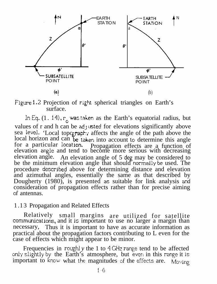
in Eq. (1.13) in place of cos & where @’ is the difference inlongitude between subsatellite point and earth station. Cos Z is theangular distance of a great-circle path for the special case that oneof the end points is at O deg latitude (Fig. 1.2). Also theexpression follows from the “law of cosines for sides” of sphericaltrigonometry (Jordan, 1986). The angle a of Fig. 1.2 for an earth-space path can be determined by using

cos a = tan 0’ cot Z (1.17)

another rdation applying to a right spherical triangle (Jordan,1986). The angle a is shown in Fig. 1.2a for an earth stationlocated to the east of the subsatellite point. The azimuth anglemeasured from north in this case would be i 80 deg + a. For anearth station location to the west of the subsatellite point as in Fig.1.2b, the azimuth angle from north is 180 deg - a. AS an example,calculations for Boulder, Colorado. latitude 40 deg N, longitude105 deg W and for Satcom-2, located at 119 deg W, with cos Z =c o s 4 0 d e g t i m e s c o s M deg = 0.743~ give d = 3’L668 kmelevation angle 9 = 41.46 deg, and azimuthal angle = 201.2 deg.

%UBSATELLITEPOINT

EARTHSTATION

N

a

8’

+’SUBSATELLITE JPOINT

(aj (b)

Figure 1.2 Projection of right spherical triangles on Earth’ssurface.

h Eq. (1. 14), rc was !a~en as the Earth’s equatorial radius, butvalues of r and h can be ad.; usted for elevations significantly abovesea level. ‘Local topo rap!!’; affects the angle of the path above thelocal horizon and can L taken into account to determine this anglefor a particular locatim. Propagation effects are a function ofelevation angle and tend to become more serious with decreasingelevation angle. An elevation angle of 5 deg may be considered tobe the minimum elevation angle that should normally be used. Theprocedure describ~d above for determining distance and elevationand azimuthal angles, essentially the same as that described byDougherty (1980), is presented as suitable for link analysis andconsideration of propagation effects rather than for precise aimingof antennas.

b

B

1.13 Propagation and Related Effects

Relatively small margins are ut i l ized for satel l i tecommunicatiorls$ and it is important to use no larger a margin thannecessary, Thus it is important to have as accurate information aspractical about the propagation factors contributing to L even for thecase of effects which might appear to be minor.

Frequencies in rough] y the 1 to 4 GHz range tend to be affectedmly slightly by the Earth’s atmosphere, but everi in this ran~e it isimportant to know what the magnitudes d the effects are. Mo’;ing \

..1

It

.“

. .

to higher frequencies, attenuation and noise due to rain, clouds, andatmospheric gases increase, These effects may become limitingfactors abcve i O GHz. The ionospheric effects of Faraday rctation,amplitude and phase scintillation, and absorption, on the other hand,become increasingly significant with decreasing frequency.

Depolarization or cross polarization may occur in propagationthrough the atmosphere or in reflection from terrestrial features.These terms refer to a degradation or change in polarization asfrom purely vertical linear polarization to linear at an angleslightly different from vertical. This latter polarization isequivalent to a combination of vertical and horizontal polarization.The power converted to the orthogonal polarization may interferewith a channel having that polarization and make less effective thepractice of frequency “reuse” (using the same frequency for twoorthogonal polarizations in this case). An effect that is importantto ranging and navigation systems is the excess range delay, abovethat encountered in propagation through a vacuum, that isencountered in propagation through the Earth’s ionosphere andtroposphere.

Electromagnetic radiation emitted by the atmosphere, animportant part of sky noise, is not strictly a propagation effect butis closely related and increases when attenuation incrwases. As isevident from Eqs. (1. 11) and (1. 12), T~ys affects system

performance directly, Sky noise contributes to T~Vs. When using a

low noise receiving system, only a slight increase’in sky noise mayincrease T significantly. It is important to know TSys Sys , as well

as L, as accurately as practical.

A few references of a general nature, concerning either satellitesystems or propagation effects, are appropriate for mention here.A comprehensive treatment of satellite communication engineeringhas been presented by Miya (1981), and Freeman (1981) includessatellite systems, as well as HF radio, line-of-sight terrestrialsystems, and troposcatter systems, in his TelecommunicationTransmission Handbook. Thompson (19? 1) prepared an Atmospheric~ransmission Handbook< covering the range. from 3 kHz to 3,000

z. Recent references on satellite communications have beenprovided by Feher (1983), Pratt and Bostian (1986), and Pritchardand Sciulli (1986). Hall (i 979) presented a summary of

1-7

tropospheric effects on radio communication, and lppolito (1986)concentrated on the role of radio wave propagation in satellitecommunciations. NASA Reference Publication 1082 (Ippolito,Kaul, and Wallace, 1983) treats propagation effects at frequenciesabove 10 GHz, but many of the concepts and much of the materialpresented is pertinent to a broader range of frequencies. Evans(1986) has reviewed the development of international satellitecommunications over the past two decades and considered likelytrends in satellite systems as these may evolve with relation tofiber-optic cables.

1.2 FREQUENCY ASSIGNMENTS AND APPLICATION BELOW 10GHZ

Frequencies below 10 GHz are used for a variet of purposesinvolving earth-space paths as shown in Table 1.1. ?he categoriesof service are actually little diffe~nt for frequencies above 10GHz. This handbook treats propagation effects between 100 MHzand 10 GHz, and a listing of frequency allocations for space servicein this band is given in Table 1.2. The entries in this table arefrom the Final Acts of the World Administrative Radio Conference,Geneva, l= Volume 1 E (ITU2, which com rises North and $0

PAtlantic and acific Oceans. Allocations for Region 1 (Europe,Africa, and Northern Asia) and Re ion 3 (Southern Asia and the

5South Pacific, including Australia an New Zealand) are similar but .differ in details. The reference includes numerous ~ footnotes givinginformation about exceptions for particular countries and eriods,

$but information from the footnotes is omitted from Table 1. unlessotherwise indicated. For brevity we use Uplink and Downlink inplace of Earth-to-space and space-to-Earth as in the originalpublication. Allocations are also given in the Manual of R ulations

,,, +and Procedures for Fedeml Radio Fre uenc =gement~~) and in the~~niu ations.

The INTELSAT satellite system uses frequencies near 6 GHzfor the uplink and fre uencies near 4 GHz for the downlink, and

Eallocations used by INT LSAT are included in Table 1.2 as entriesfor fixed satellites. Note, that a number of space services utilizelower frequencies. Included among these services are space

P.AA

1-8 . ..A

It

. .

Table 1.1 Satellite Services (ITU, 1982, Revised 1985)

Aeronautical Mobile Satellite

Aeronautical Radionavigation Satellite

Amateur Satellite

Broadcasting Satellite

Earth Exploration Satellite

Fixed Satellite

Inter Satellite

Land Mobile Satellite

Maritime

Maritime

Mobile Satellite

Radionavigation Satellite

Meteorological Satellite

Mobile Satellite

Radiodetermimtion Satellite

Radionavigation Satellite

Space Operations

Standard Frequency and Time Signal Satellite

1-9

m

Table 1.2 Frequency Allocations for Space Services (ITU, 1982,Revised 1985).

PFre uency Services

(~Hz)

4 3 7 - 1 3 8

138 -143.6i43.6 -143.65143.65-144

144-146149.9-150.05

267-272272-273322 -328.6399.9-400.05400.05-400.15400.15-401

401-402

.

402-403

406 -406.1406.1-410460-470608-614

620-790

S ace Operations and Reseanh (Downlink)Jeteomdogical Satellite (Downlink)

Space Reseamh (Downlink)

Space Research (Downlink)

Space Research (Downlink)

Amateur Satellite

Radionavigation Satellite

Space Operation (Downlink)

Space Operation (Downlink)

Radio Astronomy -

Radionavigation Satellite

Standard Frequency and Time Signal Sat.

Meteorological Satellite (Downlink)Space Reseamh and Operation (Downlink)

Space Operation (Downlink)Earth Exploration Satellite (Uplink)Meteorological Satellite (Uplink)

Earth Exploration Satellite (Uplink)Meteorological Satellite (Uplink)

Mobile Satellite (Uplink)

Radio Astronomy

Meteorological Satellite (Downlink)

Rad~o Astronomy (Footnote 688)Mobile Satellite (Uplink)

Broadcasting Satellite (Footnote 693)

l-io

Table 1.2 Frequency Allocations for Space Services (continued).

/306 -890942-960

1215-1240.- 1240-1260

1370.-1400

1400-1427

1427-1429

1525-1530

1530-1535. . .

1535-1544

1544-1545”

1545-1559

1559-1610

1626.5 -1645.5

1645.5 -1646.5

1646.5-1660

1660 -1660.5

1660.5 -1668.4

Mobile Satellite (Footnotes 699,700,70 1)

Mobile Satellite (Footnotes 699, 701 )

Radionavigation Satellite (Downlidd

Radionavigation Satellite (Downlink)

Space Reseamh (Passive)Earth Exploration Satellite (Footnote 720) -

Radio Astronomy (1420 MHz H line)Earth Exploration Satellite (Passive)Space Research (Passive)

Space Operation (Downlink)

Space Operation (Downlink)Earth Exploration Satellite

Space Operation (Downlink)Maritime Mob. Sat. (Downlink, Foot. 726)Earth Exploration Satellite

Maritime Mobile Satellite (Downlink)

Mobile Satellite (Downlink)

Aeronautical Mobile Satellite (Downlink)

Radionavigation Satellite (Dowdink)

Maritime Mobile Satellite (Uplink)

Mobile Satellite (Uplink)

Aeronautical Mobile Satellite (Uplink)

Aeronautical Mobile Satelllte (Uplink)Radio Astronomy

Radio AstronomySpace Researvh (Passive)

1-11

Table 1.2 Frequency Allocations for Space Services (continued).——

Frequency Services(MHz)

!668.4 -1670

1670-1690

1690-1700

1700-1710

1718.8 -1722,2

1758-1850

1770-17902025-2110

2110-2120

2200-2290

2290 ‘ 2300

2500-25352500-2655.

2655-2690

2690-2700

3400-3500

Radio Astronomy

Meteorological Satellite (Downlink)

Meteorological Satellite (Downlink)

Meteorological Satellite (Downlink)

Radio Astronomy (Footnote 744) .

Space Operation and Research(Uplink, Footnote 745)

Meteorological Satellite (Footnote 746)

Space Operation and ResearchEarth Exploration Satellite (Footnote 747)

S ace Reseamh (Deep Space Uplink)(footnote 748)Space Resea&h and Operation (U link)

f(Until 31 Dec. i 990, Footnote 7 9)Space Research and OperationEarth Exploration Satellite (Footnote 750)

Space Research (Deep Space Downlink)

Mobile Satellite (Downlink, Footnote 754)

Fixed Satellite (Downlink)Broadcasting Satellite

Fixed Satellite (Downlink and Uplink)Broadcasting SatelliteEarth Exploration Satellite (Passive)Radio Astronomy and Space Research

Earth Exploration Satellite (Passive)Radio Astronomy and Space Reseamh

Fixed Satellite (Downlink)

r!

c

1-12~1.-

—

. .

Table f.2 Frequency Allocations for Space Services (continued).

Free.&y Services

3500-3700 Fixed Satellite (Downlink)3700-4200 Fixed Satellite (Dovdink)

4202 Standard Frequency and Time (Downlink)(Footnote 791)

4500-4800 Fixed4800-4900 Radio4990-5000 Radio

Space

Space

Space

Fixed

5250-5255

5650-5725

5725-5850

5830-5850

5850-5925

5925-7025

6427

7125-7155

7145-7190

7250-7300

7300-7450

7450-7550

Satellite (Downlink)

Ast”kxmomy

AstronomyReseanh (Passive)

Research

Reseamh (Deep Space)

Satellite (Uplink)

Amateur Satellite (Downlink)(Footnote 808)

Fixed Satellite (Uplink)

Fixed Satellite (Uplink)

Standard Frequency and Time (Uplink)(Footnote 791 )

Space Opemtion (Uplink, Footnote 810)

S ace Research (Deep Space Downlink)(#’ootnote811 )

Fixed Satellite (Downlink)Mobile Satellite (Dowdink)

Fixed Satellite (Downlink)Mobile Satellite (Downlink)

Fixed Satellite (Downlink)Meteorological Satellite (Downlink)Mobile Satellite (Downlink)

1-13

m

Table 1.2 Frequency Allocations for Space Service (continued).

Frequency.— —

Services(MHz)

7550- 77s0 Fixed Satellite (Downlink)Mobile Satellite (Downlink)

7900-7975 Fixed Satellite (Uplink)Mobile Satellite (Uplink)

7975-8025 Fixed Satellite (Uplink)Mobile Satellite (Uplink)

8025-8175 Fixed Satellite (Uplink)Earth Exploration Satellite (Downlink)Mobile Satellite (Uplink)

8175- 821S

8215-8400

8400-8450

8450-85009975-10025

Earth Exploration Satellite (Uplink)Fixed Satellite (Uplink)Meteorological Satellite (Downlink)Mobile Satellite (Uplink)

Earth Exploration Satellite (Downlink)Fixed Satellite (Uplink)Mobile Satellite (Uplink)

Space Research (Deep Space Uplink)

Space Reseamh (Downlink)

Meteorological Satellite (Footnote 828)

?s

a

.I1.1

research, involving the use of telemetry for transmittin~ data to the— .Earth, and s ace operations, including ‘the functionscommand. Fhe frequency ranges of 2110 to 21202300 MHz, 5650 to 5725 MHz, and 8450 to 8500as being for deep-space research.power system for collecting solarenergy tosystem is

of [racking andMHz, 2290 toMHz are listed

‘ Plans for the proposed satelliteenergy called for transmission of

implementation of such athe Earth at 24~0 MHz. btiquestionable.

1-14

.

\

Parties involved in the development of land-mobile satellitesystems in the United States and Canada have wanted to use portionsof the 806-890 MHz band that have been held in ~serve, but an FCCdecision of July 28, 1986 allows only for L-band operation in theUnited States for land-mobile satellite service. The Aeronauticaland Mobile Satellite services will share on an equal basis (co-primary) the 1549 .5-1558.5 MHz band for space to mobileplatform transmission and the 1651-1660 band for mobileplatform to space transmission. The Aeronautical Mobile Satelliteservice is designated as the primary occupant and Mobile Satelliteservice will be a seconds

?service, operated on a non-interference

basis, in the 1545-1549. MHz band for space to mobile platformoperation with 1646-1651 MHz used for mobile platform to spaceoperation, Some of the 806-890 MHz band that was previously heldin reserve was allocated to the Public Safety Radio Service, andfour MHz (849-85 1 and 894-896) were kept in reserve.

The version of Table 1.2 of this edition includes a number ofentries that were not in the original 1979 version of the table,especially in the 7250-8175 MHz range where Mobile Service wasadded to the previous listin s.

\NTIA (1986) shows the allocations

in this frequency range to e for governmental use in the UnitedStates.

Listings or logs of operational or planned geostationarysatellites are published from time to time in the COMSAT Reviewand elsewhere. The texts by Pratt and Bostian (1986) and Pritchardand Sciulli (1986) also include information of this type.

1.3 STRUCTURE OF THE EARTH’S ATMOSPHERE .

Earth-space paths traverse both the Earth’s troposphere andionosphere, and the characteristics of the atmospheric regions arethus pertinent to satellite communications.

Troposphere

T e m p e r a t u r e d e c r e a s e s with increasing altitude in thetroposphere, but temperature inversion laye= provide exceptions tothis general characteristic. The thickness of the troposphere variesbut it extends to about 10 km over the poles and 16 km over theequator. The upper limit of the troposphere is known as the

1-15

—

tropopause. A plot of atmospheric temperature versus altitude isshown in Fig. 1.3.

Atmospheric pressure tends to decrease exponentiallywith altitude in accordance with

P-h/H= po e (1.18)

where h is the height above a reference level where the pressure isPO* The scale height H is not a constant as it is a function of

temperature T, the average mass of the molecules present, and theacceleration of gravity g as indicated by

H = kT/mg

where k is Boltzmann’s constant.(1.19)

The rate of change of temperatm with altitude in a dryatmosphere in an adiabatic state (involving no input or loss of heatenergy) is given by dT/dh = -9.8 deg C/km. The dry adiabatic rateof change of temperatm with height is of interest because thestability or instability of the atmosphere is determined in large partby the relative values of the actual rate of change of temperaturewith altitude and the dry adiabatic rate. If the actual la se rate of

fthe atmosphere (rate of decreasi of temperature with a titude ) is9.8 deg C/km, a pa~el of air that is originally in equilibrium withits surroundings and which is then moved upwards or downwardswill tend to remain in equilibrium, at the same temperature as itssurroundings. The parcel of air will then not be subject to anrestraining or accelerating force. Such a lapse rate of temperatureis referred to as neutral. If the actual lapse rate of the atmosphereis greater than 9.8 deg C/km, a rising parcel of air will tend tocool onlyat the adiabatic rate and be warmer than its surroundings.As a result it will be lighter than the air around it and will beaccelemted still further upwards, The air in this condition isunstable. If the lapse rate is less than 9.8 deg C/km, a parcelmoved upwards will tend to cool at the adiabatic rate and be coolerthan its surroundings, Thus it is subject to a force that inhibits Pvertical motion. A lapse rate less than 9.8 deg C\km is a stablelapse rate.

..1

1-16

!)

.

30(

. .

20(

10C

0

$

ATHERMOSPHERE

\

MESOPHERE

)STRATOSPHERE

TROPOSPHERE

- - - --- --- - - -Zw 4UU 600 800 1000

T (K)

Figure 1.3 Atmospheric temperature versus altitude (values fromU.S. Standard Atmosphere, 1976).

In an inversion layer temperature increases with altitude, andsuch a layer is highly stable. All vertical motions are stronglyinhibited inan inversion layer, and pollution emitted below the layertends to be confined below it. If a source of water vapor existsbelow an inversion layer, the vapor tends to be confined below thelayer also with the result that a large decrease in index ofrefraction may be encountered in upward passage through aninversion layer. The occurrence of inversion layers may have animportant effect on low-angle earth-space communication paths(Sees. 3.2 and 3.3).

Inversions tend to develop at night and in the winter, especiallyunder conditions of clear sky as in the desert at night and in thearctic and subarctic in winter. Inversions may also form whenwarm air blows over a cool surface such as an ocean surface.Subsiding air is another cause of inversions, and this type ofinversion is common because descending air is associated withdeveloping or sempermanent anticyclones. The Pacific coast of theUnited States lies along the eastern edge of a semipermanentanticyclone that forms in the Pacific; this occurrence is a majorfactor in causing the pollution problems of the Los Angeles area.

Model atmosphe~s have been developed to present the bestavailable estimates of the average values of pressure, density,temperature, and other parameters. One such model atmosphere isthe U.S Standard Atmosphe~ (1976). Tempemture tends todec~ase on the average at a rate of 6.5 deg C/km, which is lessthan the dry adiabatic rate. When rainfall occurs at the Earth’ssurface a transition to ice and snow particles tends to occur at theheight where the C) deg C isotherm is reached. Water dro s cause

Rmuch higher attenuation than do ice particles and snow, so t e O degC isotherm marks the upper boundary of the region where mostattenuation due to precipitation occurs.

Stratosphere, Mesosphe~, Thermosphere

Above the troposphere temperature increases with height, to amaximum near 50 km, as a result of the absorption of solarultmwiolet radiation by ozone (Fig. 1.3). This region of increasingtempemture with hei ht is known as the stratosphere.

!The

mesosphe~, a region o decreasing temperature with height, occursabove the stratosphere and extends to about 85 km.

F

. .

D

.

.

1-18

Above 85 km is the thermosphere, in which temperature againincreases with height as a result of the dissociation of atmosphericgases by solar ultraviolet radiation, Above 300 km temperatureschange little with height for a considerable distance. Below about100 km temperatn changes little with time, but the temperatureabove 120 km may vary by nearly a factor of 3 to 1, being highestin the daytime near the peak of the ii-year sunspot cycle.

The characteristic of the thermosphere of most importance tosatellite communication is not the temperature structure itself butthe ionization that. occ~ there. On the basis of the ionization, theregion is known as the ionosphere. The ionosphere has a lowerlimit of about 60 km, and it thus includes part of the mesosphere aswell as the thermosphen.

Ionosphere

The ionosphe~ extends from about 60 km to a not very welldefined upper limit of about 500 to 2000 km above the Earth’ssurface, As geostationary satellites operate at an altitude of about35,786 km, transmissions to and from these satellites pass throughthe entire ionosphe~. The ionosphere, which is ionized by solarradiation in the ultraviolet and x-ray frequency ranges, is an ionizedgas or plasma containing free ~lectrms and positive ions so as to beelectrically neutral. Only a fraction of the molecules are ionized,and large numbers of neutral molecules are also present. It is thefree electrons that affect electromagnetic wave propagation in thefrequency range considered in this report (100 MHz to 10 GHz),

Because different portions of the solar spectrum are absorbed atdifferent altitudes, the ionosphere consists of several layers orregions. The layers are not sharply defined, distinct layers, and thetransition from one to the other is generally gradual with no verypmmounced minimum in electron density in between. Representativeplots of electron density are shown in Fig. 1.4. Two good sources offurther information about the ionosphere are those by Rishbeth andGarriot (1 969) and Ratcliffe (1969).

D Region

The D region, the lowest of the ionospheric regions, extendsfrom approximately 50 to 90 km with the maximum electron

1-19

1000

500

MAXIMUM OF‘ S U N S P O T —

SUNSPOT CYCLE

0[ I , ,1 t 1, 1 , , ,,1 1

104 105 106 107

(a) DAYTIME

1000

I ct ILICDqT cYCLEfMINI”MUM OF ‘ laulwrw

SUNSPOT CYCLE

500 I I \ l \ I

103

ELECTRON CONCENTRATION (eiectrons/cm3)

01 , 1 I .I102 “,.3

104 105 106 107ELECTRON CONCENTRATION N (electrons/cm3

(b) NIGHTTIME

Figure 1.4 Electron densit distribution at the extremes of the/’sunspot cycle ( rom Hanson, W. B., “Structures of the

Ionosphere” in Johnson, F.S. (cd.), SatelliteEnvironment Handbook, Stanford U. Press, 1965).

i’-.W

,-

—

1-20.-

electron density of about 109/m3 occurring between 75 and 80 kmin the daytime. At night electron densities throughout the D regiondrop to vanishingly small values.

As the electron concentration in the D region is very low, ittends to have little effect on high-frequency waves. However,attenuation in the ionosphere occurs mainly through collisions ofelectrons with neutral particles, and as the D region is at a lowaltitude many neutral atoms and molecules are present and thecollision frequency is high. Therefore transmissions in the AMbroadcast band are highly attenuated in the day time in the Dregion, but distant reception improves at night when the D regiondisappears.

E Re~ion

The E region extends from about 90 to 140 km, and the peakelectron concentrate ion OCCH between about 100 and 110 km.Electron densities in the E region vary with the i i-year sunspotcycle and maybe about 10*i/m3at noonat the minimum of the solarcycle and about 50 percent greater at the peak of the cycle.Electron concentrations drop by a factor of about 100 at night,Intense electrical currents flow in the equatorial and auroralionospheres at E-region altitudes, these currents being known asequatorial and equatorial electrojets. Radio waves are scatteredfrom electron density structure associated with the electrojets atfrequencies up to more than 1000 MHz. Backscatter echoes from-the auroral electrojets indicate the regions of occurrence of auroraand are referred to as radio aurora. The phenomem of sporadic E,thin, sporadic, often discontinuous layers of intense ionization,occurs in the E region, at times with electron densities well above10 *2/m3. The E layer is useful for communications, as HF wavesmay be reflected from the E layer at frequencies which are afunction of time of day and period of the sunspot cycle. By causinginterference between VHF stations, sporadic E tends to be anuisance.

F Regio~

The F region has the highest electron densities of the normalionosphere. It somet irnes consists of two parts, the F, and F2

layers. The Fi layer largely disappears at night but has peak

densities of about 2.5 x 10ll~ms at noon at the minimum of thesolar cycle and 4 x lC)lt,/ms at noon at the peak of the solar cycle.The F2 layer has the highest peak electron densities of theionosphere and the electron densities there remain higher at nightthan in other regions. The peak electron density is in the 200-. to400-km height range and may be between about 5 x 10 i l,\m3 and 2 x10*2/m3 in the daytime and between 1 x 10~1/m3 and 4 x 1011 /m3

at night. Reflection from the Fz layer is the major factor in HFcommunications which formerlydistance, especially transoceanic,

handled a largecommunications,

fraction of long-

Plasmasphere and Magnetosphere

The upper limit of the ionosphere is not weciselv defined butfor the p~poses of space communications m~y be taken as 2000km, this being the upper limit for significant Faraday rotation(Seco2.2). Above the ionosphere i s the plasmasphere orprotonosphere, which has an electron content of about 10 percent ofthe ionospheric content in the daytime “and up to 50 percent of theionospheric content at night, as defined along an earth-space path.

The Earth’s magnetic field is confined inside an elongated cavityin the solar wind, that extends to about 10 earth radii in thedirect ion towards the Sun and has a long tail extending to about50 earth radii or farther in the opposite direction. The boundary of .this cavity is known as the magnetopause, and the region inside theboundary, above the ionosphere, is known as the magnetosphere. Themagnetosphere can be defined as the region in which the Earth’sfield dominates the motion of charged particles, in contrast to theionosphere where collisions play a major role. The Van Allenradiation belts, discovered in 1958 by use of Explorer 1, are in themagnetosphere. The plasmasphm-e, usually considered to be abovethe ionosphere (or above 2000 km), is below the Van Allen beltsand is the lowest region of the magnetosphere. The plasmasphere isbounded on the upper side at about 4 earth radii at the equator by theplasmapause where the plasma density drops by a factor of 10 to100 or from about. 108\m3 to 10b/m3.

[

r.&.

1-22

I I

.

kre~ularities and Disturbed Conditions

A brief description has been provided of the ionospheric layers.

.-

. .

Consideration of ~he ionosphere” can be separated into the quietionosphere and ionospheric disturbances and irregularities, as occurat times of magnetic storms and essentially eve

%night to some

degree in the auroral and equatorial ionospheres. oth propagationin the quiet ionosphe~ and the effects of disturbances andirregularities are conside~d in the following Chap. 2.

1.4 NATURAL REGIONS OF THE EARTH, A GLOBAL VIEW OFPROPAGATION EFFECTS

The uneven heating of the Earth’s surface by the Sun, therotation of the Earth and the consequent Coriolis forwe, and surfacefeatures of the Earth determine a characteristic pattern of windover the Earth, See, for example, a text on meteorology such asthat by Dorm (1975), p. 238. In good measure because of thispattern, corresponding characteristic patterns of climate,ecos terns, vegetation,z

tropospheric refractivity (Sec. 3.1 ), andrai all (Chap. 4) also occur over the surface of the Earth. Thelivin portions of ecosystems are referred to as biotic communities,

Land t major terrestrial biotic communities are known as biomes.For pmctical purposes the biomes can be referred to simply asnatural regions. Maps of the natural regions of all the continentsare included in the Aldine Unive=it Atlas (Fullard and Darley,1969). ‘+7 and geographicalThe clim-lca , eco oglca ,characteristics of a ~gion are closely related and are pertinent tosatellite communications. Areas of tropical forest, which arerapidly disappearing, can be expected to have heavy rainfall and ahigh atmospheric water vapor content. The Arctic, on the otherhand, has low precipitation and low values of water vapor.

Global models for estimating rainfall statistics have beendeveloped and are discussed in Sec. 4.3.3, where rain rate ~gionsare shown in Figs. 4.8 - 4.10 and Figs. 4.13 - 4.15. The regionsshown are in rough correspondence with the natural regions ofFullard and Darley (1969) and also with the Koppen system forclassifying climates (Trewartha, 1968). The global models are notvery detailed, however, and advantage should be taken of any moredetailed information that may be available.

1-23

.

REFERENCESAllen, C. W., Astrophysical Quantities. London: University of

London, Athlone Press, 1978.Dom, W. L., Meteormlo

+’4th Ed. New York: McGraw-Hill, 1975.

Dou herty,F

A Consol idated Model for UHF/SHFelecommunicatiom Links Between Earth and Synchronous

Satellites, NTIA Report 80-45, U.S. Dept. of Commerce,Au~. 1980.

Evans,” J. V., “Twenty years of international satellitecommunications,” Radio Sci., VO1.21, pp. 647-664, July-Aug.1986.

Feher, K., o “ . . .

Fm-!e;z;Ft:y% ‘atell’te’Yr$83stat10nrentice-f-lall i

Te ecommunlcatlom Transmission Handbook, 2ndEd., New York: Wiley,

Fullard, H. and H.C. Aldine Universi~_ Atlas.Chicago: Aldine, 1969. ——. ._ ———— -- ————

Hall, M. P.M., Hfects of the Troposphere on Radio Communications.Stevena e,

3 ‘K ‘NPeter Peragrinus for IEE, 19 /9

Ippolito, L. ., R.D~n Ka~~ R.G. Wallace, Pro a ation Effec~s*ma~fHandbook for Satellit

_onipairments on z Satellite Links withTechni ues for System Design, NASA Reference Pub.1082 (0?). Washington, DC: NASA Headquarters, 1983.

Ippolito, L. J., Radiowave Propagation in Satellite Communications.New York: Van Nostrand Reinhold, “~9~

ITU (International Telecommmicatiom Union), Final Acts of theWorld Administrative Radio Conference, Geneva, 19~~1,.~~982 R -

Jordan, E.C. red. ‘~ns ef), Reference Data for En inee~: Radio,—-*T

_ -~~ ~~~”~;};~’ (Also in e’Reference Data for Radio Engineers, Sixth Ed., 1975.)

Miya, Satellite Communication~Sf33-chome, shinjuku~->~f~ A1$l 3-2:

NTIA (National Telecommunications and InformationAdministmtion), Manual of Re u.lations and Procedures for

-asiton, DC ~~~~Fedeml Radio Fre uenc ~nagement.9 M~~

!3

.!?

1-24

.&

Pratt, T.and C.W. Bostian, Satellite Communications. New York:Wilev. 1986.

Pritchar&’ W. L. and J.A. Sciulli, Satellite Communication SystemsEn ineerinWA

Englewooe Cliffs, NJ : Prentice-Hall, 1986.Rat~l e , An Introduction to the Ionosphere a n d——- -—-——— -- —-— —- -—- -——-

Ma netos he& Cambridge: ~ambridge University Press, 1972..—-— — ————- ———

R i s h - 0. K. Garriott, Introduction to IonosphericPhvsics. New York : Academic Press, 1969. —

ThommW.I., Atmospheric Transmission Handbook, Report No.DOT-TSC-NASA- ~ 1-6. Cambrid~e, MA: TransportationS y s t e m s C e n t e r . F e b . i 9 7 1 . -

Trewartha, G. T., An Introduction to Climate. New York: McGraw-Hill, 1 9 6 8 . —

U.S. Standard Atmosphere, 1976, sponsored by NOAA, NASA,USAF. Washington, DC: Supt. of Documents, U.S. GovernmentPrinting Office, 1976.

. .

1-25